Adaptive Moving Mesh Modeling for Two Dimensional ...people.ku.edu/~wzhuang/research/paper/AMSCM05-383-HZ.pdf · Contemporary Mathematics Adaptive Moving Mesh Modeling for Two Dimensional

Contemporary Mathematics

Adaptive Moving Mesh Modeling for Two Dimensional

Groundwater Flow and Transport

Weizhang Huang and Xiaoyong Zhan

Abstract. An adaptive moving mesh method is presented for numerical sim-

ulation of two dimensional groundwater flow and transport problems. A se-

lection of problems are considered, including advection dominated chemical

transport and reaction, solute transport from contamination sources, transport

of nonaqueous phase liquids (NAPLs) in an aquifer, and coupling of ground-water flow with NAPL transport. Numerical results show that the adaptivemoving mesh method is able to capture sharp moving fronts and detect theemerging of new fronts.

1. Introduction

Groundwater resources are vital to the natural environment, social welfare,and economic health. In the past two decades, numerical simulation has proved tobe an effective tool for simulating and predicting behaviors of chemical contami-nation in the subsurface that can degrade groundwater quality. Indeed, a varietyof algorithms and software have been developed for the numerical simulation ofgroundwater flow and transport, e.g., see [25, 31] and references therein. Mean-while, the quest for more accurate and efficient numerical methods remains active.This is especially true for problems exhibiting sharp moving fronts, for which con-ventional methods tend to produce oscillatory solutions and excessive numericaldispersion in regions around sharp fronts.

It has been amply demonstrated that, by placing more mesh nodes in the re-gions around sharp fronts than in the rest of the domain, mesh adaptation providesan effective tool in reducing numerical dispersion and oscillation while enhanc-ing the efficiency and accuracy of numerical simulation. Roughly speaking, meshadaptation can be cast into two main categories, the refinement method and the dy-namic or moving mesh method. The first type of method is conceptually simpler. Itachieves mesh adaptivity by adding or removing mesh nodes locally. The refinementmethod has been successfully applied to a number of groundwater problems in oneand two dimensions. For example, Yeh et al. [29] combine the method of character-istics with local mesh refinement and effectively avoid the numerical dispersion and

1991 Mathematics Subject Classification. 65M50, 65M60, 86A05.

c©0000 (copyright holder)

1

2 WEIZHANG HUANG AND XIAOYONG ZHAN

oscillation problem in solving advection-dispersion equations. Trompert [26] applieslocal-uniform-mesh refinement to modeling transport in heterogeneous media.

On the other hand, the moving mesh method [11, 14, 23] achieves mesh adap-tivity by relocating the node positions while keeping the number of mesh nodes andthe mesh connectivity fixed throughout the entire solution process. Since the sizeof computation and data structure are kept fixed, it is much easier to implementthe moving mesh method than the refinement method. Moreover, the moving meshmethod often works better because the relocation of node positions improves thealignment of mesh elements with the solution and thus the simulation accuracy.Unfortunately, it has been known that it is difficult to formulate a reliable movingmesh method in multi-dimensions. So far, the moving mesh method has been suc-cessfully applied to groundwater modeling only in one dimension; see [8–10,17,30].

Progress has been made recently in developing more reliable moving mesh meth-ods in multi-dimensions. The development has mainly focused on the variationalapproach where the node positions are obtained by minimizing a functional measur-ing some difficulty in approximating the physical solution. Such a functional can beformulated as the energy functional of harmonic mappings [3,7,20,28] or based on aJabobian weighting [18], interpolation error estimates [12, 16], or a combination ofvarious mesh properties [1,2]. The reader is also referred to [4] for brief comparisonof variational-type moving mesh methods with those based on mesh velocity.

In this work, we focus on a particular variational-type moving mesh method,the so-called moving mesh PDE (MMPDE) approach developed by Huang et al.[14, 15]. With this approach, adaptive moving meshes are generated as imagesof a fixed computational mesh in the auxiliary domain through a time dependentcoordinate transformation. The transformation is obtained as the solution of thegradient flow equation of an adaptation functional which is related to the well-known equidistribution principle [6] and measures the difficulty in approximatingthe solution. Since the mesh nodes are continuously relocated and dynamicallyadapted to solution behavior, the MMPDE moving mesh method provides an idealadaptive strategy to capture evolving sharp fronts without using a large number ofgrid points. In [17], the method has been used to model a range of one dimensionalgroundwater problems, including of advection dominated chemical transport andreaction, non-linear infiltration in soil, and the coupling of density dependent flowand transport.

The objective of this paper is to investigate the applicability of the MMPDEmoving mesh method to two dimensional groundwater flow and transport problems.Although the moving mesh method has been successfully applied to a number of onedimensional groundwater problems [8–10, 17, 30], there lacks in published work intwo dimensions. Moreover, it is far from clear that the method is necessarily able tocapture sharp two dimensional moving fronts. This is because two dimensional mov-ing fronts have far more complicated structures and thus more difficult to simulateand track. For demonstration purpose, a range of problems common in groundwa-ter flow and transport are considered. They include advection dominated chemicaltransport and reaction, solute transport from contamination sources, transport ofnonaqueous phase liquids (NAPLs) in an aquifer, and coupling of groundwater flowwith NAPL transport.

The paper is organized as follows. The MMPDE moving mesh method and itsimplementation are presented in section 2. In section 3, the groundwater problems

MOVING MESH MODELING FOR GROUNDWATER FLOW AND TRANSPORT 3

are described. The simulation results using the adaptive moving mesh method arealso given in the same section. Finally, the summary and comments are given inSection 4.

2. The MMPDE moving mesh method

The MMPDE moving mesh method is developed in [14] in one dimension and in[15] for multi-dimensional problems. The basic idea is to define the time-dependentcoordinate transformation needed for generating adaptive meshes as the solutionof an MMPDE (moving mesh PDE), which in turn is defined as the gradient flowequation of an adaptation functional measuring the difficulty in approximating thephysical solution. The physical PDE is discretized and integrated with the quasi-Lagrange approach where the effect of mesh movement is reflected by extra termsinvolving mesh velocity in the transformed physical PDE.

For the clarity of presentation, the MMPDE moving mesh method is describedfor the following simplified version of the advection-dispersion-reaction equation(ADRE), one of typical mathematical models describing chemical transport in thesubsurface:

(2.1) R∂C

∂t=

∂

∂x

(

D∂C

∂x

)

+∂

∂y

(

D∂C

∂y

)

− V1

∂C

∂x− V2

∂C

∂y− λRC,

where C = C(t, x, y) is the concentration of a certain type of chemical, D =D(t, x, y) is the dispersivity, V = (V1(t, x, y), V2(t, x, y)) is the Darcy velocity, R isthe retardation factor, and λ is the reaction factor. It should be emphasized thatthe method can be straightforwardly applied to other systems.

2.1. Spatial discretization on a moving mesh. In a moving mesh method,the mesh is generated as the image of a uniform logical mesh under the coordinatetransformation (denoted by x = x(t, ξ, η), y = y(t, ξ, η)) from the logical domain(Ωc) to the physical domain (Ω). As a common practice, we choose the logicaldomain as the the unit square, i.e., Ωc = (0, 1)× (0, 1). Given two positive integersJ and K, let ∆ξ = 1/J and ∆η = 1/K. With the uniform logical mesh beingdenoted by

(2.2) ξj = j∆ξ, ηk = k∆η j = 0, ..., J, k = 0, ...,K

the moving mesh can be written as

(2.3) xj,k(t) = x(t, ξj , ηk), yj,k(t) = y(t, ξj , ηk) j = 0, ..., J, k = 0, ...,K.

Finite differences are used for the spatial discretization of equation (2.1). Tothis end, (2.1) is first transformed from the physical coordinates to the logical ones.Let

c = c(t, ξ, η) = C(t, x(t, ξ, η), y(t, ξ, η)).

Then, (2.1) can be written in the new coordinates as

(2.4) R∂c

∂t=

∂

∂x

(

D∂c

∂x

)

+∂

∂y

(

D∂c

∂y

)

− (V1 − xt)∂c

∂x− (V2 − yt)

∂c

∂y− λRc,

where (xt, yt) is the mesh velocity. Note that the partial derivatives with respectto x and y in (2.4) should be understood through the chain-rule, viz.,

(2.5)∂

∂x= ξx

∂

∂ξ+ ηx

∂

∂η,

∂

∂y= ξy

∂

∂ξ+ ηy

∂

∂η,


with the transformation relations being given by J = xξyη − xηyξ and

(2.6)

[

ξx ξy

ηx ηy

]

=

[

xξ xη

yξ yη

]−1

=1

J

[

yη −xη

−yξ xξ

]

.

The approximation of the partial derivatives using central finite differences on theuniform logical mesh is standard. For example,

∂c

∂x

∣

∣

∣

∣

j,k

=

(

ξx

∂c

∂ξ+ ηx

∂c

∂η

)∣

∣

∣

∣

j,k

≈ ξx|j,kcj+1,k − cj−1,k

2∆ξ+ ηx|j,k

cj,k+1 − cj,k−1

2∆η,

where ξx|j,k and ηx|j,k are calculated through (2.6). Some cautions may be neededwhen discretizing the second order derivatives. Consider the first term on the right-hand side of (2.4). In the new coordinates it reads as

∂

∂x

(

D∂c

∂x

)

= ξx

∂

∂ξ

(

Dξx

∂c

∂ξ+ Dηx

∂c

∂η

)

+ ηx

∂

∂η

(

Dξx

∂c

∂ξ+ Dηx

∂c

∂η

)

.

To obtain a compact and stable scheme, we use half-point differences for approxi-mating the outer differentiation,

∂

∂x

(

D∂c

∂x

)∣

∣

∣

∣

j,k

≈ ξx|j,k∆ξ

[

(

Dξx

∂c

∂ξ+ Dηx

∂c

∂η

)∣

∣

∣

∣

j+ 1

2,k

−(

Dξx

∂c

∂ξ+ Dηx

∂c

∂η

)∣

∣

∣

∣

j− 1

2,k

]

+ηx|j,k∆η

[

(

Dξx

∂c

∂ξ+ Dηx

∂c

∂η

)∣

∣

∣

∣

j,k+ 1

2

−(

Dξx

∂c

∂ξ+ Dηx

∂c

∂η

)∣

∣

∣

∣

j,k− 1

2

]

.

The remaining differentiation can be approximated by the standard central differ-encing and averaging, e.g.,

∂c

∂ξ

∣

∣

∣

∣

j,k± 1

2

≈ 1

2

[

cj+1,k − cj−1,k

2∆ξ+

cj+1,k±1 − cj−1,k±1

2∆ξ

]

,

∂c

∂η

∣

∣

∣

∣

j± 1

2,k

≈ 1

2

[

cj,k+1 − cj,k−1

2∆η+

cj±1,k+1 − cj±1,k−1

2∆η

]

.

It is noted that the effect of mesh movement is reflected in the transformedequation (2.4) via the terms containing mesh velocity (xt, yt). For this reason,(2.4) is often said to be of the quasi-Lagrange form. With this quasi-Lagrangeapproach, there is no need for interpolation of the physical variable from the oldmesh to the new mesh. This is in contrast to the so-called mesh rezoning approach,where the physical variable is interpolated from the old mesh to the new mesh andthe physical PDE is discretized and integrated on the new mesh (that is consideredfixed in the current time step); see [11,20] for more discussion on this approach.

2.2. The MMPDE approach of mesh movement. The idea of the MM-PDE approach is to determine the time-dependent coordinate transformation neededfor generating adaptive meshes as the solution of an MMPDE, which in turn isdefined as the gradient flow equation of an adaptation functional measuring thedifficulty in approximating the physical solution. To measure the difficulty in the


numerical approximation of the solution, we define the so-called arc-length monitorfunction as

(2.7) M(x, y) = I + ∇C(∇C)T =

[

1 + C2x CxCy

CxCy 1 + C2y

]

.

Generally we expect that the mesh is generated such that it closely satisfies the so-called equidistribution principle or the mesh density is approximately proportionalto the square root of the determinant of the monitor function (e.g., see [16]). In thissense, the monitor function (2.7) places more mesh nodes in the regions of largegradient of the solution C. It is known that the arc-length monitor function is thesimplest but not the best for all cases. The reader is referred to [16] for a moresophisticated definition of the monitor function based on interpolation error.

Given the monitor function, the adaptation functional is defined for the inversecoordinate transformation as

(2.8) I[ξ, η] =1

2

∫

Ω

(

(∇ξ)T M−1∇ξ + (∇η)T M−1∇η)

dxdy,

where ∇ = (∂/∂x, ∂/∂y) is the gradient operator. The MMPDE is then defined [13]as the gradient flow equation of I[ξ, η],

(2.9)∂ξ

∂t=

1

τp∇ ·

(

M−1∇ξ)

,∂η

∂t=

1

τp∇ ·

(

M−1∇η)

,

where p = p(t, x, y) is a positive function (cf. its definition in (2.11)) and τ > 0 isa user-prescribed parameter for adjusting the time scale of mesh movement. Thefinal form of the MMPDE is obtained by interchanging the roles of the independentand dependent variables in (2.9),

∂x

∂t=

1

τp

[

a11

∂2x

∂ξ2+ 2a12

∂2x

∂ξ∂η+ a22

∂2x

∂η2+ b1

∂x

∂ξ+ b2

∂x

∂η

]

,

∂y

∂t=

1

τp

[

a11

∂2y

∂ξ2+ 2a12

∂2y

∂ξ∂η+ a22

∂2y

∂η2+ b1

∂y

∂ξ+ b2

∂y

∂η

]

,(2.10)

where

u =1

J

[

yη

−xη

]

, v =1

J

[

−yξ

xξ

]

, J = xξyη − xηyξ,

a11 = uT M−1

u, a12 = uT M−1

v, a22 = vT M−1

v,

b1 = −uT

(

u

∂M−1

∂ξ+ v

∂M−1

∂η

)

, b2 = −vT

(

u

∂M−1

∂ξ+ v

∂M−1

∂η

)

,

p =√

a211 + a2

22 + b21 + b2

2.(2.11)

Central finite differences are used to discretize the mesh equation (2.10) on theuniform logical mesh. In our computation, τ is taken as τ = 0.01, and this valueseems to work well for all the tested cases .

2.3. Time integration and solution procedure. In principle, the physicalPDE (2.4) and the MMPDE (2.10) can be integrated in time either simultane-ously or alternately. However, alternating solution seems more realistic in multi-dimensions since it voids the highly nonlinear coupling of the mesh and physicalsolution and preserves many structures such as ellipticity and sparsity in each ofthe mesh and physical PDEs. The following alternating procedure is used in our


computations. Here, ∆t is the time step size associated with the physical PDE and∆tmesh for that related to the MMPDE.

Alternating Procedure: Assume that the physical solution cn, themesh (xn, yn), and a time step size ∆tn are given at time t = tn.

(i) Compute the monitor function Mn(x, y)=M(tn, x, y) using cn and (xn,yn).The solution derivatives used in M are calculated using a gradient recov-ery technique similar to that developed by Zienkiewicz and Zhu [32, 33]based on the nodal values of the computed solution. Mn is understood asa continuous function in the sense of interpolation.

(ii) Integrate the MMPDE (2.10) over the time period [tn, tn + ∆tn] usingvariable step size ∆tmesh,n and monitor function M(x, y) = Mn(x, y).The MMPDE is discretized in time using the backward Euler schemewith the coefficients a11, a12, a22, b1, and b2 being calculated at tn. Morethan one sub-step may be needed for the integration to reach t = tn+∆tn.When this happens, the monitor function is updated for each sub-step vialinear interpolation. The obtained mesh is denoted by (xn+1, yn+1).

(iii) Integrate the physical PDE (2.4) with a fixed or variable step size. Theequation is discretized in time using the Singly Diagonally Implicit Runge-Kutta scheme [5]. The mesh and mesh velocity are calculated using linearinterpolation:

x(t) =t − tn∆tn

xn+1 +tn + ∆tn − t

∆tnxn, y(t) =

t − tn∆tn

yn+1 +tn + ∆tn − t

∆tnyn.

(iv) When a variable step size is used in step (iii), the physical PDE may

actually be integrated over a smaller step ∆tn < ∆tn. In this case, themesh at the actual new time level tn+1 = tn + ∆tn should be updated as(xn+1, yn+1) := (x(tn+1), y(tn+1)).

(v) Go to the next step with the step size predicted by the physical PDEsolver.

3. Applications

Example 3.1: Advection dominated chemical transport and reac-tion. Contaminant in form of ions, molecules, or particles undergoes multiple andcomplicated processes including transport, chemical, and biological ones in waterenvironment. The transport process is mainly due to advection and dispersion.The chemical process covers acid-base reactions, solution, volatilization, precipita-tion, solute reactions, oxidation-reduction reactions, hydrolysis reaction, isotropicreactions, adsorption, and desorption. The biological process covers bacterias andvirus activities. A quantitative description of these processes is prerequisite to thesuccessful protection of water quality. The advection-dispersion-reaction equation(ADRE), Eq. (2.1), is one of most commonly used mathematical models describ-ing these processes in geohydrology [19]. The equation can become advection-dominated or dispersion-dominated depending on the magnitude of the aquiferpermeability and Darcy velocity. The challenge in the numerical solution of thisequation is to capture the chemical transport and reaction front without intro-ducing erroneous instability and numerical dispersion while maintaining reasonablecomputational efficiency. The physical domain is taken as Ω = (0, 1)× (0, 1) in ourcomputations.


We now consider a case which essentially is one-dimensional. We choose thistest example because it has the exact solution and can be used to verify the com-puter code. Moreover, the one dimensional version of the ADRE with the sameexact solution has been used as an example for testing the one dimensional MM-PDE moving mesh method in [17].

For this case, the physical parameters are taken as D(t, x, y) = D = 10−5,V1(t, x, y) = V = 1, V2(t, x, y) = 0, and R = 1.1, and λ = 1.1. The initial andboundary conditions are defined as(3.1)

C(0, x, y) = 0, C(t, 0, y) = 1, C(t, 1, y) = C∗,∂C

∂y(t, x, 0) =

∂C

∂y(t, x, 1) = 0,

where C∗ is a constant taken as the value at x = 1 of the exact solution [19,27]

C(x, t) =1

2exp

(

V x

2D

)

[

exp

(

−√

V 2 + 4DλRx

2D

)

erfc

(

x −√

V 2 + 4DλRt/R√

4Dt/R

)

+ exp

(√V 2 + 4DλRx

2D

)

erfc

(

x +√

V 2 + 4DλRt/R√

4Dt/R

)]

.

A typical adaptive mesh and the solution obtained thereon are shown in Fig. 1.The chemical reaction front is captured with the adaptive moving mesh. The resultsare in good agreement with the one dimensional ones obtained in [17].

Figure 1. Example 3.1. Adaptive moving mesh (first row) andcomputed solution (second row) for ADRE.


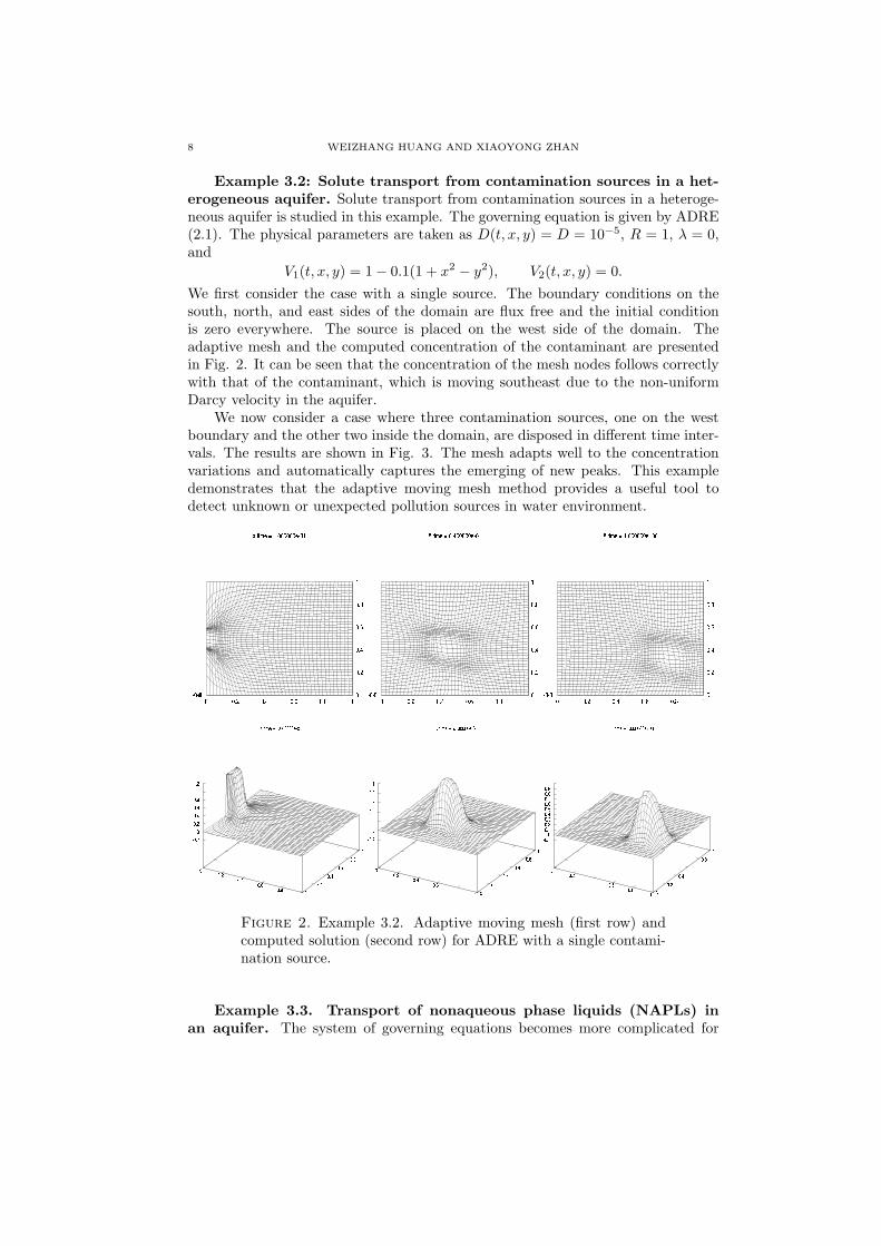
Example 3.2: Solute transport from contamination sources in a het-erogeneous aquifer. Solute transport from contamination sources in a heteroge-neous aquifer is studied in this example. The governing equation is given by ADRE(2.1). The physical parameters are taken as D(t, x, y) = D = 10−5, R = 1, λ = 0,and

V1(t, x, y) = 1 − 0.1(1 + x2 − y2), V2(t, x, y) = 0.

We first consider the case with a single source. The boundary conditions on thesouth, north, and east sides of the domain are flux free and the initial conditionis zero everywhere. The source is placed on the west side of the domain. Theadaptive mesh and the computed concentration of the contaminant are presentedin Fig. 2. It can be seen that the concentration of the mesh nodes follows correctlywith that of the contaminant, which is moving southeast due to the non-uniformDarcy velocity in the aquifer.

We now consider a case where three contamination sources, one on the westboundary and the other two inside the domain, are disposed in different time inter-vals. The results are shown in Fig. 3. The mesh adapts well to the concentrationvariations and automatically captures the emerging of new peaks. This exampledemonstrates that the adaptive moving mesh method provides a useful tool todetect unknown or unexpected pollution sources in water environment.

Figure 2. Example 3.2. Adaptive moving mesh (first row) andcomputed solution (second row) for ADRE with a single contami-nation source.

Example 3.3. Transport of nonaqueous phase liquids (NAPLs) inan aquifer. The system of governing equations becomes more complicated for


Figure 3. Example 3.2. Adaptive moving mesh (first row) andcomputed solution (second row) for ADRE with multiple contam-ination sources.

multiphase flow and transport in groundwater environment; e.g. see [21, 24] andreferences therein. Here we consider a specific case where nonaqueous phase liq-uids (NAPLs) are dissolved into the aqueous phase [22]. The physical process isdescribed by two PDEs, one for the volumetric fraction of NAPL or NAPL content,

(3.2)∂θn

∂t= −kna (C∗

a − Ca)

ρn

,

and the other for the NAPL dissolved in water,

(3.3)∂(θaCa)

∂t= ∇ · (D∇Ca − qaCa) + kna (C∗

a − Ca),

where the subscripts “a” and “n” represent the aqueous and nonaqueous phases,respectively, the superscript “∗” indicates an equilibrium condition with the com-panion phase involved in the mass transfer, θ = θ(t, x, y) is the volumetric fraction,Ca = Ca(t, x, y) is the concentration of the NAPL dissolved in water, ρ is density,kna is a mass transfer coefficient representing a mass transfer process referenced toa loss by the nonaqueous phase and a gain by the aqueous phase, qa is water flux,and D is the dispersivity. It is noted that θn + θa = n, where n is the porosity con-sidered to be constant here. The reader is referred to [22] for the derivations of thegoverning equations and the corresponding initial and boundary conditions. Thevalues of the physical parameters are taken as those given in Table 15.1 of [22]. Inparticular, the water flux is taken as a constant vector in the x-direction. The pa-rameter values are representative of conditions encountered in the two-dimensionalphysical experiements. The physical scenario of this case is that the aqueous phase


is being flushed from the left boundary and the dissolved NAPL is being elutedfrom the right boundary. The left and right boundary conditions are a specifiedflux for the aqueous phase, while the top and bottom boundary conditions are no-flow. The initial residual NAPL saturation and other parameters are homogeneous,a typical laboratory condition, except that a perturbation in the residual NAPLsaturation near the left boundary where a portion of the boundary is NAPL free,indicating that a clean water is flushing in. The development of this perturbationinto a dissolution profile is then observed.

The obtained results are shown in Fig. 4 for mesh evolution, NAPL, anddissolved NAPL in water. It can be observed that a clean inflow from the westboundary washes out NAPL and reduces dissolved NAPL in water in a channelzone with time. The movements of the front and the boundary of the channel arecaptured correctly with the adaptive mesh. Once again the results show that theadaptive moving mesh method holds a great promise for solving multiphase flowand transport problems such as NAPL dissolution.

Example 3.4. Coupling of groundwater flow and NAPL transport.A more realistic modeling of the NAPL transport requires consideration of thecoupling with the water flow. In this situation, in addition to equations (3.2) and(3.3), another equation is needed for the aqueous phase pressure pa = pa(t, x, y),viz.,

(3.4) 0 = ∇ ·(

k kra

µ(∇pa − ρag∇x)

)

+

(

1

ρa

− 1

ρn

)

kna(C∗

a − Ca),

where k is permeability, kra is relative permeability, µ is viscosity, g is the gravityconstant, and x is the vertical coordinate. Unlike the previous example, the waterflux in the equation (3.3) is now given by Darcy’s law,

qa = −k kra

µ(∇pa − ρag∇x) .

The values of other physical parameters are taken from Table 15.1 of [22]. Similarphenomena can be observed from the computational results (cf. Fig. 5). Thisseems reasonable since the water flux remains stable and has a similar profile asthe one used in Example 3.3 as far as the water pressure gradient is maintained.

4. Summary and comments

The MMPDE (moving mesh PDE) moving mesh method developed in [14, 15]has been presented and applied to the numerical simulation of groundwater flow andtransport problems. A range of problems have been considered, including advectiondominated chemical transport and reaction, solute transport from contaminationsources, transport of nonaqueous phase liquids (NAPLs) in an aquifer, and couplingof groundwater flow with NAPL transport. Numerical results have demonstratedthat the MMPDE moving mesh method is able to capture sharp moving fronts anddetect the emerging of new fronts. This consolidates the findings in a previouswork [17] for one dimensional groundwater problems.

It should be pointed out that the investigations presented in this work are stillat a preliminary stage and more work has yet to be done. For example, we haveused a simple adaptation functional (2.8) and the arc-length monitor function (2.7)for mesh movement. For more precise control of mesh adaptation and for better


Figure 4. Example 3.3. Adaptive moving mesh (first row), NAPL(second row), and dissolved NAPL in water (third row) for theNAPL problem.

simulation accuracy, it would be better to use more sophisticated functionals andmonitor functions such as those developed in [12,16] based on interpolation error.

Acknowledgements

The work was partially supported by the National Science Foundation throughgrants DMS-0074240 and DMS-0410545 and by the Kansas Geological Survey. Thesimulations were performed with a SGI-Origin 2000 multi-processor computer inthe Kansas Center for Advanced Scientific Computing, The University of Kansas.It is acknowledged that L. Zheng participated in this investigation at the earlystage.


Figure 5. Example 3.4. Adaptive moving mesh (first row), NAPL(second row), dissolved NAPL in water (third row), and aqueousphase pressure (fourth row) for the NAPL-flow coupling problem.


References

1. J. U. Brackbill, An adaptive grid with directional control, J. Comput. Phys. 108 (1993), 38 –50.

2. J. U. Brackbill and J. S. Saltzman, Adaptive zoning for singular problems in two dimensions,

J. Comput. Phys. 46 (1982), 342 – 368.

3. W. Cao, W. Huang, and R. D. Russell, An r-adaptive finite element method based upon

moving mesh pdes, J. Comp. Phys. 149 (1999), 221 – 244.

4. , Approaches for generating moving adaptive meshes: location versus velocity, Appl.

Numer. Math. 47 (2003), 121 – 138.

5. J. R. Cash, Diagonally implicit runge-kutta formulae with error estimates, J. Inst. Math.

Appl. 24 (1979), 293 – 301.

6. C. de Boor, Good approximation by splines with variable knots, Spline Functions and Ap-

proximation Theory (A. Meir and A. Sharma, eds.), Birkhauser Verlag, Basel und Stuttgart,

1973, pp. 57 – 73.

7. A. S. Dvinsky, Adaptive grid generation from harmonic maps on riemannian manifolds, J.

Comput. Phys. 95 (1991), 450 – 476.

8. A. Gamliel and L. M. Abriola, A one-dimensional moving grid solution for the coupled non-

linear equations governing multi-phase flow in porous media. 1: Model development, Int. J.

Numer. Meth. Fluids 14 (1992), 25 – 45.

9. , A one-dimensional moving grid solution for the coupled nonlinear equations govern-ing multi-phase flow in porous media. 2: Example simulations and sensitivity analysis, Int.

J. Numer. Meth. Fluids 14 (1992), 47 – 69.10. G. Gottardi and M. Venutelli, Moving finite element model for one-dimensional infiltration

in unsaturated soil, Water Resour. Res. 28 (1992), 3259 – 3267.11. D. F. Hawken, J. J. Gottlieb, and J. S. Hansen, Review of some adaptive node-movement

techniques in finite element and finite difference solutions of PDEs, J. Comput. Phys. 95

(1991), 254 – 302.12. W. Huang, Measuring mesh qualities and application to variational mesh adaptation, to ap-

pear in SIAM J. Sci. Comput.

13. , Practical aspects of formulation and solution of moving mesh partial differentialequations, J. Comput. Phys. 171 (2001), 753 – 775.

14. W. Huang, Y. Ren, and R. D. Russell, Moving mesh partial differential equations (MMPDEs)based upon the equidistribution principle, SIAM J. Numer. Anal. 31 (1994), 709 – 730.

15. W. Huang and R. D. Russell, A high dimensional moving mesh strategy, Appl. Numer. Math.26 (1997), 63 – 76.

16. W. Huang and W. Sun, Variational mesh adaptation II: error estimates and monitor func-tions, J. Comput. Phys. 184 (2003), 619 – 648.

17. W. Huang, L. Zheng, and X. Zhan, Adaptive moving mesh methods for simulating one-

dimensional groundwater problems with sharp moving fronts, Int. J. Numer. Meth. Engng.54 (2002), 1579 – 1603.

18. P. M. Knupp, Jacobian-weighted elliptic grid generation, SIAM J. Sci. Comput. 17 (1996),

1475 – 1490.

19. T. Lee, Applied mathematics in hydrology, Lewis Publishers, 1999.20. R. Li, T. Tang, and P. W. Zhang, Moving mesh methods in multiple dimensions based on

harmonic maps, J. Comput. Phys. 170 (2001), 562 – 588.21. C. T. Miller, G. Christakos, P. T. Imhoff, J. F. McBride, J. A. Pedit, and J. A. Trangen-

stein, Multiphase flow and transport modeling in heterogeneous porous media: Challenges

and approaches, Adv. Water Resour. 21 (1998), 77 – 120.

22. C. T. Miller, S. N. Gleyzer, and P. T. Imhoff, Numerical modeling of napl dissolution fingering

in porous media, Physical nonequilibrium in soils modeling and application (H. M. Selim andL. Ma, eds.), Ann Arbor Press, Chelsea, Michigan, 1998.

23. K. Miller and R. N. Miller, Moving finite elements I, SIAM J. Numer. Anal. 18 (1981), 1019– 1032.

24. T. F. Russell, Modeling of multiphase multicontaminant transport in the subsurface, Rev.

Geophys. 33 (1995), 1035 – 1047, Supplement 2.25. D. R. Shier and K. T. Wallenius, Applied mathematical modeling: A multidisciplinary ap-

proach, Chapman & Hall/CRC, London, Boca Raton, 2000.


26. R. Trompert, Local-uniform grid refinement and transport in heterogeneous porous media,

Adv. Water Resour. 16 (1993), 293 – 304.

27. E. J. Wexler, Analytical solutions for one-, two-, and three-dimensional solute transport in

ground-water systems with uniform flow, U.S. Geological Survey, Book 3, Techniques of Water-

Resources Investigations, 1992, p. 190.

28. A. M. Winslow, Adaptive mesh zoning by the equipotential method, Tech. Report UCID-19062,

Lawrence Livemore Laboratory, 1981.

29. G. T. Yeh, J. Chang, and T. E. Short, An exact peak capturing and oscillation-free scheme to

solve advection-dispersion transport equations, Water Resour. Res. 28 (1992), 2937 – 2951.

30. P. A. Zegeling, J. G. Verwer, and J. C. H. Van Eijkeren, Application of a moving grid method

to a class of 1D brine transport problems in porous media, Int. J. Numer. Meth. Fluids 15

(1992), 175 – 191.

31. C. Zheng and G. D. Bennett, Applied contaminant transport modeling: Theory and practice,

Van Nostrand Reinhold, New York, 1995.

32. O. C. Zienkiewicz and J. Z. Zhu, The superconvergence patch recovery and a posteriori error

estimates. part 1: The recovery technique, Int. J. Numer. Methods Engrg. 33 (1992), 1331 –

1364.

33. , The superconvergence patch recovery and a posteriori error estimates. part 2: Error

esimates and adaptivity, Int. J. Numer. Methods Engrg. 33 (1992), 1365 – 1382.

Department of Mathematics, The University of Kansas, Lawrence, KS 66045, USA

E-mail address: [email protected]

Kansas Geological Survey, The University of Kansas, Lawrence, KS 66047, USA

E-mail address: [email protected]

Documents

Adaptive Moving Mesh Modeling for Two Dimensional ...people.ku.edu/~wzhuang/research/paper/AMSCM05-383-HZ.pdf · Contemporary Mathematics Adaptive Moving Mesh Modeling for Two Dimensional