r-'.

NASA Technical Memorandum 84336 lil.[)Da U'C - ?<L330

ASA-TM 8 .- 4336 19840003 109

Adaptive Inverse Control for Helicopter Vibration Reduction Stephen A. Jacklin

September 1983

NI\S/\ National Aeronautics and Space Administ ration

y

! / 1 (1983

U\NGLEY R~Sr.AR Elllrfl'< L BRARY NASA

HA i?TON, VIRGINIA

J

https://ntrs.nasa.gov/search.jsp?R=19840003109 2018-06-28T08:05:55+00:00Z

NASA Technica l Memorandum 84336

Adaptive Inverse Control for Helicopter Vibration Reduction Stephen A. Jack li n, Ames Research Center, Moffett Field, California

NJ\S/\ National Aeronautics and Space Administration

Ames Research Center Moffett Field . California 94035

SUMMARY

The reduction or alleviation of helicopter vibration will reduce main t enance requirements while at the same t ime increase ride quality and helicopter reliability . In forward fl ight, the helicopter ' s fuselage vibration spectrum tends to be dominated b y multiples of the "N/REV" component. This paper presents a way to use the method of adaptive inverse control to identify, in real- time, a controller capable of gen­erating N/REV vibra tion of opposite phase to cancel the uncontrolled N/REV vibra­tion component . The control cons i dered in this paper will be that of multicyclic feathering of blade pitch .

INTRODUCTION

In forwar d fligh t, asymme trical airflow through the produces a fuselage vibration spectrum which tends to be the N/REV component ; where "N" is the number of blades N cycles of vibration per rotor revolution. The N/REV dynamics may be modeled in the locally linear sense as:

rotor disk of the helicopter domina ted by multiples of in the rotor producing helicopter vibration

.6Z (j) = T (j) M (j) (1)

Here, [Z(j)] is a (p x 1) vector whose elements are the N/REV sine and cos ine coef ­ficien ts of the Fourier transform of data taken from fuselage accelerometers . The vector [ 8 (j)] is an (m x 1) vector whose elements are the selected sine and cosine coefficients of the higher harmonic blade pitch. The local linear model postulates that within a short time interval the changes in the harmonic coeff icients of cyclic pitch are linearly related t o the changes in the harmonic coefficients of vibration. The tra nsfer matrix describing this linear relationship is "T."

One solution to the vibration control problem would be to identify T, find its inverse (for m = p), and then form the optimal control as :

Z(j) is the total sensed (measured) N/REV vibration. The vector .68 (j) is the change in multicy'clic control necessary to induce a vibration component of opposite phase to cancel the sensed vibration. The minus sign thus signifies opposite phase .

Figure 1 shows this control system. This approach to vibration control is limited to transfer matrices which are square, as presented thus far, but can be easily generalized for the nonsquare case.

This paper presents the method of adaptive inverse control as a means to simul­taneously identify the inverse of the transfer matrix and to find the vibration feed­back gain matrix . This method uses the least mean square (LMS) algorithm of Widrow

--'

and Hoff (ref. 1) to identify the inverse of the transfer matrix. Thereby, no inver­sion is required . Hence, the adaptive inverse control scheme is computa tionally v ery efficient .

REGULATOR DESIGN WITH ADAPTIVE INVERSE CONTROL

In this paper , the LMS algorithm and the method of adaptive inver se control pre­sented by Windrow, McCool, and Medoff (ref . 2) are extended to solve the multiple ­input/multiple-output helicopter vibration control problem . The necessary input command to the con troller in this case is a vector whose elements are the uncon trol led componen t s of N/REV vibration, changed in sign. In this manner the feedback com­mands giv en t o the controller represent the vibration desired to cancel .

The resultant controller ar rangement is shown in figure 2 . The controller has been placed afte r the pla nt to form an adaptation error vector . The commanded change in multicyclic pitch at step j is 6 8 (j) . Referring to figure 3, it is seen that when 68 (j) is inputted to the helicopter, a corresponding change in vibration, 6Z(j) , results:

6Z (j) = [T (j) ] M (j ) (3)

This 6Z(j) is s ubse que ntly mUltiplied by C , the controller ma trix . If C is th e inverse of the transfer matrix , T, then [C] * 6Z(j) should equal the original com­ma nded change in pitch, 68 (j). This is usually not quite e qual to the original cha nge in pitch because of e rrors in [C] ide ntification and is thus denoted with a " ha t" symbol, 68 (j) .

Adapta tion Error M (j) M (j)

e (j) M (j) [C (j) ] 6 Z (j)

M (j) [C(j) ] [T(j) ] [ Lle (j) ] (4 )

Cl early , this error will be minimized when the con troller ma trix , C, is the inverse of T . This error vector is then use d by the LMS algorithm in steepest descent form t o update the estima t e of the inverse tr a nsf er ma trix, C. This algorithm is an ite rative identification technique which makes changes in the C (inverse plant) ma trix e lements proport ional to the gradient of the expected value of the mean s qu are error signal with r espec t to the current e stimate of C,

It will be shown that a n unbiase d es timate of this gradien t is g ive n by ,

(5)

The steepest descent (LMS - SD) algorithm fo r calculating each row "i" of the contr oller matrix is then shown to be:

(6 )

2

LMS ALGORITHM IMPLEMENTATION

The LMS algorithm (ref. 1) is the iterative estima tion algorithm which we will use here to identify the inverse of the plant (helicopter) transfer matrix . In this sec tion, the LMS algorithm and the method of adaptive inverse control presented by Widrow, McCool, and Medoff (ref . 2) will be extended to solve t he multiple-input, multiple-output helicopter vibration control problem . This extension will be made by identifying the inverse transfer matrix in a row-b y-row fashion . In this manner, the single weight vector originally LMS identified by Widrow and Hoff (ref . 1) now becomes a matrix of weights. The LMS algorithm will be adap ted to make row-by-row corrections to the current row estimate s of the inverse matrix. Using the "steepest descent" approach, these corrections will be made proportional to the gradient of the expected mean square estimation error vector, with respect to the current row esti­mate values. In this section we will de fine the terminology used and explain the meaning of the previous statement.

For each row "i" of the controller matrix at time step "j " we have:

and the square of this error as :

Here, 68 (j) is the ith element of the control vector fed into the helicopter plant (T).

( 7)

(8)

The LMS algorithm is an iterative identification technique which makes changes in the C (inverse plant) matrix elements proportional to these estimat ion error signals. For each row of the controller matrix, the steepest descent update can be written as:

(9)

This equation states that the current row estimate is equal to the previous value of the estimate plus a cor rection term. The correction term is zero when the identifi­cation err or is zero.

"E[efU)] " denotes the "expected value" of the error squared, or the mean square error. V{E[et(j)] } denotes the gradient of the mean square error signal respect to the current estimate of C. That is,

with

(10)

An expression of this gradient for the multiple-input, multiple-outout (MIMO) case will be presented. Note that if the row error is large , a large change will be made to the row estimate of the inverse. If the error is small, a small change will be made. The stability constant , ks' governs the stability and rate of convergence of this method, as will be shown .

3

The feature which makes the LMS algorithm so efficient is the elaborate manner in which the gradient of the mean square error is estimated. This method is now discussed in the context of identifying the inverse plant matrix, C . The gradie nt

of the mean square error can be approximated for one time step (Ref. 1) as:

(11)

Then by noting that the gradient of the error can be expressed as:

(1 2)

we may express the gradient of the mean square error as:

(1 3 )

I t is important to r e alize that in this expression ~ 8 (j) is an (n x 1) vector, ~ZT(j ) is a (1 x m) vector, and hence the gradient is not a vector, but an (n x m) ma trix .

Al though surprisingly simple in form, this approximation to the gradient is unb i ased . To s e e this, we note that the square error (for each row i) may be expresse d as:

The mean square error can then be found by taking the expected value of the e rror squa r e d :

wh e r e the c overiance matrices have been defined as

an d

T 4l i (Z, 8 )

(14)

(1 5)

(16 )

4l (Z,Z) = E[ ~ Z(j) ~ZT(j)] (17)

If we n ow differentiate the expected value of the error squared with respect to C, we f ind tha t

V{ E[e 21.o (j)]} = - 2¢~(Z, 8 ) + 2C~(j) 4l (Z,Z) (18 )

1. 1.

whi ch is in agreement with the gradient estimate we had before:

4

--- --- -- ---

(19)

Furthermore, by setting the gradient expression in equation (18) equal to zero, we see that each row of the C matrix should converge to the corresponding row of the inverse of T in an ordinary least squares sense:

(20)

as this is the same solution as would be obtained for the ordinary least square error solution.

Thus by using

(21)

as the gradient es timate of the mean square error, the LMS-SD algorithm fo r each row "i" of the controller matrix is:

C~ (j + 1) 1

(22)

Stability and rate of convergence are determined by the selection of the stabil­ity constant, k s ' Considerations governing the selection of ks will now be discussed.

SELECTION OF STABILITY CONSTANT ks FOR ALGORITHM STABILITY AND CONVERGENCE

It has been shown thus far that we can find an unbiased estimate of the mean square error gradient for steepest descent utilization. The convergence properties of the steepest descent technique will now be discussed . Specifically, there is a nee d to know when the method can be guaranteed to converge to the true inverse of the plant, an d how long it will take to do so . Our analysis will follow that of Widrow and Hoff (ref. 1) and will be extended to incorporate the helicopter (plant) inverse identification problem.

For each row (i) of the C (inverse plant) matrix the following difference equa­tion was written for the method of steepest descent:

(23)

Taking the expecte d value of both sides of this equation we get :

5

E[CI(j+l)]

j

2ks L [I + 2k s<I>(Z,Z)]¢I(Z, 8) i=o

(24)

This equation can be put into modal form by writing the signal covariance matrix a s

(25)

where Q is the matrix composed of the eigenvectors of ~ (Z,z) and A is a diagona l ma trix whose elements are the eigenvalues of ~ (Z,z) . Substituting this int o the ab ove equation y ields:

j

E[CI(j + 1)] = [1 + 2ksQ- 1AQ]j+1C i (O) - 2ks ~ i = o

j

E[CI(j + 1)] = Q- l[1 + 2ksA]j+1QCI(O) - 2ksQ-l ~ (I + 2ksA)iQ¢ICZ, 6) i= o

Fr om this we n o t e tha t a s long a s the e l e ments of

a r e a l l l ess t han one, then the term

will conve r ge to z e r o , a nd the seco nd t e rm will c onve r ge to

j

l imit - 2ksQ- l ~ [I + 2ksA]iQct>IcZ, 6) j +oo i= O

6

- 2k Q- l s

00

l: Cl + 2ksAp)iQ ct> IcZ, 6) i=O

(26)

( 27)

J

Thus, for convergence to the correct solution by the method of steepest descent, we see that

(28)

(29)

Within these limits, the value of ks is selected with regard to the desired application. Values of ks close to zero will be less apt to be affected by random noise variations on the plant at the expense of slow adaptation. Values of ks near - l/ Amax will adapt rapidly, but will be more prone to tracking random noise after " convergence" has been achieve d, and will tend to oscillate about the correct solu­tion. The right value of ks is the one which converges at a sufficiently rapid rate, yet does not produce unacceptable steady state convergence errors. It is pos­sible to make the value of ks depend exponentially on the time step, but this will not be discussed here.

The rate of convergence may be thought of in terms of learning curve time con­stants, T . Letting rp denote the geometric ratio of the pth mode, we can say that

rp (l + 2ks Ap)

The n,

rp exp (- Tip)

1 1 1 -- + 2!T T Tp P P

or

1 Tp ::;

2k s Ap

If all eigenvalues of ~ (Z,Z) were the same, a single exponential learning curve co uld be defined. In the more general case, however, the eigenvalues will not

(30)

(31)

(3 2)

be e qual. Then the learning curve will be a f unction of all of the eigenvalues corresponding to the various normal modes. Thus, we can expect the fast modes to cause rapid initial learning , whereas the learning errors associated with the slower modes will take longer to die out and govern final convergence.

STARTING THE ADAPTIVE INVERSE VIBRATION CONTROL ALGORITHM: THE TRAINING PHASE

We have thus far established a method for iteratively correcting the estimate of the helicopter transfer matrix inverse. Yet, nothing has been said about initial conditions. At the start of the control routine, whether on the ground or in the air, a good starting value for the inverse of the helicopter transfer matrix may not

7

I ~

be known. Hence, a learning phase, termed the "training phase," is required at the start of the algorithm.

During the training phase, the blade pitch is given small perturbations and the corresponding changes in vibration are measured . These measurements are then used by the LMS-SD algorithm to correct an arbitrary i nitial value of the inverse plant matrix, C(O). Any value of C(O) may be used - for example, all elements equal to zero. No vibration control commands are generated during the training phase. In this manner, large transients in control are avoided. Hopefully, after a number of iterations, the inverse plant matrix will be accurate enough to use in the actual con trol phase.

The control phase begins when the sum of squares of the adaptat ion errors, ~ 8 - ~8 , becomes small enough . No further training is then required. The LMS - SD algorithm will update the estimate of the plant inverse transfer matrix to keep up with changes in the plant (helicopter) or changes in the operating environment .

SIMULATION OF A THREE- INPUT, THREE-oUTPUT PLANT

The LMS-SD algorithm presented in this paper was simulated for a three- state plant. An arbi trary three- by - three transfer matrix , T, was chosen to r e present the helicopter (fig . 4) . The helicopter- vibration dynamics were then modeled in the global sense by the fol lowing equations:

r,(j] [" T 1 2 r, ][, (j] [Z' (0] Z2 (J) = T21 T 22 T 2 3 8 2 (j ) + 22 (0) (33)

z 3 (j) T 31 T 3 2 T 3 3 8 3 (j) Z 3 (0)

Vibra tion at Multicyc lic con trol Uncontrolled step k input vibration

The LMS -SD update equations which identify the inverse plant transfer matrix (con­troller matrix) were then:

Ci (j + 1)

C; (j + 2) (34)

And the vibration con trol commands we re then generated b y :

(35)

8

----- I

r - ----- ----- - - .-- - - -- - _. ---

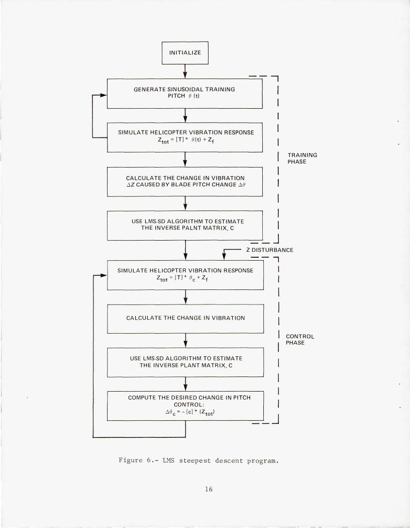
The simulation included both the training and the control phases. The effects of identification errors and changes in the operating conditions were also simulated. The overall program is diagrammed in figure 6.

From the preliminary simulation results, the LMS-SD algorithm appeared to pro­vide a very robust control system. Figures 4 and 5 illustrate some of the interest­ing results obtained. Figure 4 illustrates the typical convergence pattern for ks chosen near its midrange stability. Here the sum of the adaptation errors, 68 - £8, have been plotted versus the identification iteration cycle count . From this plot the normal modes of the system can be seen. Initial rapid convergence seemed to be produced by the fast modes, whereas final convergence appeared to be governed by the slower modes.

Figure 5 shows the behavior of LMS-SD convergence and vibration levels through the training and control phases. To simulate a sudden change in the operating condi­tions, the plant simulation values were suddenly changed by 20% and the uncontrolled vibration level was changed by 40%. The effect of these changes is shown in figure 5. The controller was able to respond in a manner to alleviate the vibration and a rather surprising feature of this robust con trol system was discovered.

The controller values did not have to converge exactly, or even very c losely, to cancel the vibration. For example, figure 5 shows that after a step disturbance in the uncontrolled vibration level, the controller may retain steady-state identifica­tion errors, while rapidly alleviating the vibration. The explanation of this robust­ness rests in part upon the identification and control phases being iterative pro­cesses. As such, the proper change in blade-pitch control can be generated by a number of linear combinations of control changes over several steps. It turned out (in simulation) that when the controller matrix was sufficiently close to the true inverse, a linear feedback combination capable of alleviating most of the vibration was generated. When the vibration level approached zero, the pitch vector was no longer altered, thus preventing complete identification of the inverse. This was as it should be, since if there is no vibration, there is no need to change the pitch­control vector. The controller matrix can then no longer be altered since the update correction term (eq. (22)) goes to zero for no uncontrolled vibration. In actual implementation, however, random noise and perturbations would most likely allow com­plete convergence to the true inverse. The significant point though is that complete convergence is not required for good vibration control .

CONCLUSIONS

The method of adaptive inverse control was presented in the context of vibration control. The theory used to derive the MIMO LMS-SD algorithm was Results of computer simulations of the inverse adaptat ion process were also and shown to indicate the validity of the results predicted by the theory. clusions verified by simulation were as follows :

helicopter given . presented The con-

1. The method of adaptive inverse vibration control can provide a very robust control system which does not require a perfect knowledge of the inverse plant matrix to alleviate vibration.

2 . The "training phase" and the LMS-SD algorithm allows the method of adaptive inverse control to be implemented without any a priori knowledge of the plant. No

9

dynamic models are required, as the training phase can quickly determine proper con­troller initial conditions .

3 . The LMS-SD algorithm is capable of adapting the controller to track changes in the flight conditions or changes in the uncontrolled vibration level. The con­troller converges quickly for moderate disturbance levels, while taking longer for larger (step) disturbances .

4 . The learning curve of the controller during the training phase was shown to be quantitatively close to that predicted by the learning curves of the normal modes.

5. The method of adaptive inverse control should have very fast on-line capa­bility, as implementation of the LMS-SD algorithm requires so few operations.

REFERENCES

1 . Widrow, B.; and Hoff, M. E., Jr.: Adaptive Switching Circuits. IRE WESCON Conference Record, pt 4, 1960, pp . 96-104.

2 . Widrow, B.; McCool, J.; and Medoff, B.: Adaptive Control by Inverse Mode ling. 12th Asilomar Conference on Circuits, Systems, and Computers, Nov . 1978, pp. 90-94 .

10

,-----

C (n x m)

CONTROLLER COpy

t::.z

(m X 1)

(n X 1)

80-1)

T (m X n)

HELICOPTER PLANT

Z

(m X 1)

Figure 1 .- An inverse controller where C is the inverse of T .

11

ZFLlGHT (m X 1)

\

I \

\

I

\

I

\

\

\

\

\

\

-- - -- ----

110 ~ DELAY .

(n X 1)

A. +'-

I _ 110 - 110 L r LMS - SD 1"'-I

(n X 1)

I A

C T I L.,. C A

(n X m) 110 .. (m X n) (n X m) 110

... I1 z .. CONT ROLLER -- HELICOPTER - CONTROLLER (n X 1)

COpy (n X 1) PLANT (m X 1)

'w + T O{j - 1) _+ ~ 0°1.,. (m X n) Zmul .. +

~ +-. HELICOPTER (m X 1)

... ZFLlGHT (n X 1)

PLANT (m X 1)

I1z

(m X 1)

Figure 2 .- An adaptive inve rse control ler where Zmul is the multicyclic control component use d to cance l the flight vibration, Zflight ·

12

\

l

---"- - _." - -

t::.. e (n x 1 )

'--- ""- -

~ DELAY

T

.. (m X n) ~

HELICOPTER PLANT

r-I I I L..

t::.. Z ~

(m X 1)

t::..e (n X 1)

, + A

LMS - SD t::..e - t::..e L ~ (n X 1)

-~

c A

(n X m) t::.. ()

CONTROLLER (n X 1)

Figure 3.- Formation of the adaptation error used by the LMS - SD algorithm to correct the estimate of the inverse plant matrix, C .

13

SUM SQUARE IDENTIFICATION

ERRORS IN C

1.5

1.0

.5

o

ks = -0.30

T FAST MODE

E( il Zil Z T)

0.17

J\. = 0.99

2.62

-0.40 < ks < 0

T MODERAT E MODE

T SLOW MODE

50 NUMBER OF ITERATIONS

100

Figure 4. - The "learning curve" of the adaptation process, or a plot of the sum square error in the controller (inverse) identifica tion versus the number of iterations from initial conditions; ks chosen near the middle of its s t ability range .

14

----- --,

SUM SQUARE OF VIBRATION .5 ELEM ENTS

VIBRATION ALLEVIATED

0 /'

1.0

T= ~ !J 1

[ 15 1.5 ~5J 3 T= 1.5 3.5 1.5

1 -0.5 1.5 1.5

SUM SQUARE OF C IDENTIF ICATION .5

ERRORS

CONTROLLER CONVERGED

/ o 50 100 150 200 I NUMBER OF ITERATIONS I /--TRAINING PHASE _I_ CONTROL PHASE~

Figure 5 .- Controller convergence properties during the training and control pha ses, along with the uncontrolled vibration . The effect of a 20% change in the plant transfer matrix , T, and a 40% change in the uncontrolled vibration.

15

J

~

'--

~

INITIALIZE

-

GENERATE SINUSOIDAL TRAINING PITCH 0 (t)

SIMULATE HELICOPTER VIBRATION RESPONSE

Ztot = [T ] * O(t ) + Zf

CALCULATE THE CHANGE IN VIBRATION d Z CAUSED BY BLADE PITCH CHANGE d 8

USE LMS-SD ALGORITHM TO ESTIMATE THE INVERSE PALNT MATRIX, C

-

--, I I

I

I I I

I I I

_J

TRAINING PHASE

.- Z DIST URBANCE , -SIMULATE HELICOPTER VIBRATION RESPONSE

Ztot = [T ) * 8e + Zf

CALCULATE THE CHANGE IN VIBRATION

USE LMS-SD ALGORITHM T O ESTIMATE THE INVERSE PLANT MATRIX, C

COMPUTE THE DESIRED CHANGE IN PITCH CONTROL:

d O e = - [e) * (Ztot)

-

-, I I

I I I I CONTROL I PHASE

Figure 6 .- LMS steepest descen t p r og r a m.

16

--- - ----

1. Report No. 2. Government Acc_ion No. 3. Recipient 's Catalog No.

NASA TM- 84336 4. Title and Subtitle 5. Report Date

ADAPTIVE INVERSE CONTROL FOR HELI COPTER Septemb e r 1983 VIBRATION REDUCTION 6. Performing Organization Code

A-9 472 7. Aut hor(s) 8. Performing Organization Report No.

Stephen A. Jacklin 10. W()(k Unit No.

9. Performing Or9"nization Name and Address T- 5484A

NASA Ames Research Center 11. Contract or Grant No .

Moffett Field, Calif . 94035 13. Type of Report and Per iod Covered

12. Sponsori ng Agency Name and Address Technical Memorandum

National Aeronautics and Space Administration 14. Sponsori ng Agency Code

Washington, D.C. 20546 505- 42- 11 15. Supplementary Notes

Point of Contact: Stephen A. Jacklin, Ames Research Center, MS 247- 1, Moffett Field, Calif . 94035. (415) 965- 6668 or RTS 448- 6668.

16. Abstract

The reduction or alleviation of helicopter vibra tion will reduce maintenance requirements while at the same time increase ride quality and helicopter reliability. In forward flight, the helicopter ' s fuselage vibra-tion spectrum tends to be dominated by multiples of the "N/REV" component. This paper presents a way to use the method of adaptive inverse control to identify, in real - time, a controller capable of generating N/REV vibration of opposite phase to cancel the uncontrolled N/REV component. The control considered in this paper will be that of multicyclic feathering of blade pitch.

17. Key Words (Suggested by Authorfs)) 18. Distr ibut ion Statement

Helicopter vibration control Unlimited Automatic control

Subject Category - 08 19. Securitv aassif. (of this report) 20. Securitv Classif. (of this page) 21 . No. of Pages 22. Price·

Unclassified Unclas s if i e d 19 AO 2

·For sale bv the National Technical Information Service, Springfield, Virginia 22161