Embed Size (px)
Citation preview
1172 IEEE TRANSACTIONS ON SYSTEMS, MAN, AND CYBERNETICS, VOL. 20, NO. 5, SEPTEMBER/OCTOBER 1990
Adaptive Image Feature Prediction and Control for Visual Tracking with a Hand-Eye Coordinated Camera
Abstraa-An adaptive method for visually tracking a known moving object with a single mobile camera is described. The work differs from previous methods of motion estimation in that both the camera and the object are moving. The objective is to predict the location of features of the object on the image plane based on past observations and past control inputs and then to determine an optimal control input that will move the camera so that the image features align with their desired positions. A resolved motion rate control structure is used to control the relative position and orientation between the camera and the object. A geometric model of the camera is used to determine the linear differen- tial transformation from image features to camera position and onenta- tion. To adjust for.modeling errors and system nonlinearities, a self-tun- ing adaptive controller is used to update the transformation and compute the optimal control. Computer simulations were conducted to veri@ the performance of the adaptive feature prediction and control. Modeling errors, image noise, and dynamics were included in the simulation to test the robustness of the proposed control scheme.
I. INTRODUCTION
N THIS AGE of mechanization, engineers are continu- I ally trying to automate dangerous and tedious human tasks. Many of these tasks require the same hand-eye coordination that allows human beings to manipulate a dynamically changing environment. Unfortunately, ma- chines have poor hand-eye coordination. Although many machines have quicker appendage response times than humans, they do not have the visual capabilities that humans do. Because of this lack of visual feedback, many tasks have been restructured so that vision usage is mini- mal. As a result, fixturing and part presentation have become key issues. Although this is an excellent tempo- rary solution, the machine hand-eye coordination prob- lem will eventually need to be solved for more complex tasks such as space robotics, vehicle guidance, and mid- flight aircraft refueling.
There are several problems associated with using exist- ing image processing equipment for real-time control. One problem is that there is often too much information in an image to be processed in real time. The human visual system appears to reduce the data flow by using task-specific scanpaths to update it's surroundings [l]. Similarly, the data in a machine vision system may be reduced by extracting specific features (such as edges, corners, and holes) from an image and using them to determine the relative position and orientation between an object and the camera [2]. This reduces the amount of information from over two million bits (for a 512x480 by 8 bit image) to maybe a few hundred features. The number of features necessary for control can be further reduced depending on the task to be performed [3].
Another problem is that searching for image features can be time consuming. This searching time could be reduced if the vision system could accurately predict where the features will be at the next sampling time. When a visual tracking task first begins, the vision system must use all a priori knowledge to recognize and locate an object. After this initial recognition stage, the image pro- cessing can be reduced to a simple verification process [41 where the image position of the object's features are continually updated. The shorter the sampling period is, the closer the image features are expected to be to the previous sampled position. However, as the sampling pe- riod increases, some form of motion prediction becomes necessary to reduce searching time.
Several authors have developed schemes for estimating three-dimensional (3-D) motion parameters (position, ori- entation, translational and rotational velocities, and accel- erations) of an object from either a finite number of features or from optical flow. An excellent review on this subject can be found in [5]. Because of the real-time control constraint, in this paper we will concentrate on feature-based motion estimation. The first feature-based methods used Point correspondences from two consecu-
Manuscript received August 5, 1989; revised April 25, 1990. This work was supported in part by an IBM Graduate Research and in Dart bv the National Science Foundation under Grant CDR 8803017 to L I
the Engineering Research Center for Intelligent Manufacturing Systems. J. T. Feddema was with the School of Electrical Engineering, Purdue
University, when this work was performed. H~ is now with the Intelli- gent Machine Principles Division 141 1, Sandia National Laboratories,
tive image frames to determine the 3-D motion parame- ters (within a scale factor for the translation) Of a rigid body [6]. Since the results were often noise sensitive, the
Albuquerque, NM 87185.
University, West Lafayette, IN 47907.
number of point correspondences required was large. Another approach used regularization to make sure the problem was well-conditioned and the changes in rotation
C. S . G. Lee is with the School of Electrical Engineering, Purdue
IEEE Log Number 9036783.
0018-9472/90/0900-1172$01.00 01990 IEEE
1173 FEDDEMA A N D LEE: ADAPTIVE IMAGE FEATURE PREDICTION
were small enough [71. As an alternative, a Kalman filter- ing approach was used to estimate three degree-of-free- dom motion using several image frames with fewer point correspondences [SI. Some knowledge of the object’s structure was assumed to be known. Models, such as the local constant angular momentum model [9], were also used to estimate the motion over several image frames. Sethi and Jain [lo] did not assume a rigid object but suggested that smooth object motion implies smooth tra- jectories of feature points in the image domain. All of these predictive schemes assume that either the camera or the object is moving, but not both.
The purpose of this paper is to estimate the position of the image feature points of a known moving object with respect to a controllable moving camera. Because we can control the camera’s position, the estimate should be based not only on past observations but also on past control inputs. This estimate may be used to speed up feature extraction and to determine appropriate controls so that the extracted image features align with the desired features.
In this paper, we analyze the dynamic model of a visual tracking system, simplify the model for real-time control, and use a self-tuning adaptive controller to adjust for parametric uncertainties. A single-input single-output auto-regressive with exogenous inputs (SISO ARX) model is used to model the motion of the part with respect to the camera in the image plane. The observed outputs are the changes in feature positions between consecutive im- age frames. The control inputs are the commanded change in feature positions used to control the camera’s position. The noise term includes nonlinearities plus disturbances caused by the moving workpiece and feature extraction errors. This term is assumed to have a nonzero mean and be uncorrelated in time. The parameters of the model are updated using the recursive least squares parameter esti- mation method. A minimum variance controller is used to minimize the expected error between the actual and de- sired observations.
The performance of the visual tracking system was evaluated by computer simulations. In the simulations, the robustness of the proposed control scheme was tested by adding modeling errors, image noise, and dynamics to the ideal system model. The simulations showed that the tracking can be improved by an order of magnitude with feature prediction. The simulations also showed that im- age noise has a predominant effect on the steady-state error.
11. SYSTEM MODEL
This section analyzes the dynamic model of a visual tracking system and suggests a reduced-order model for control. To gain a better understanding of the modeling problem, we shall first look at a single degree-of-freedom tracking problem. From this model, we will see where the noise terms are introduced and how they affect the obser- vations. This model will then be extended to a six degree-
of-freedom tracking system. Because of the coupling between the position and orientation terms, the six de- gree-of-freedom system is inherently nonlinear. By lin- earizing the system model about an operating point and expanding it in discrete form, the system can be repre- sented as a multi-input multi-output auto-regressive mov- ing-average with exogenous inputs (MIMO ARMAX) model. The number of parameters in this model which would require adaptive updating is too large for real-time computation. Therefore, a reduced-order model of the system is proposed for consideration.
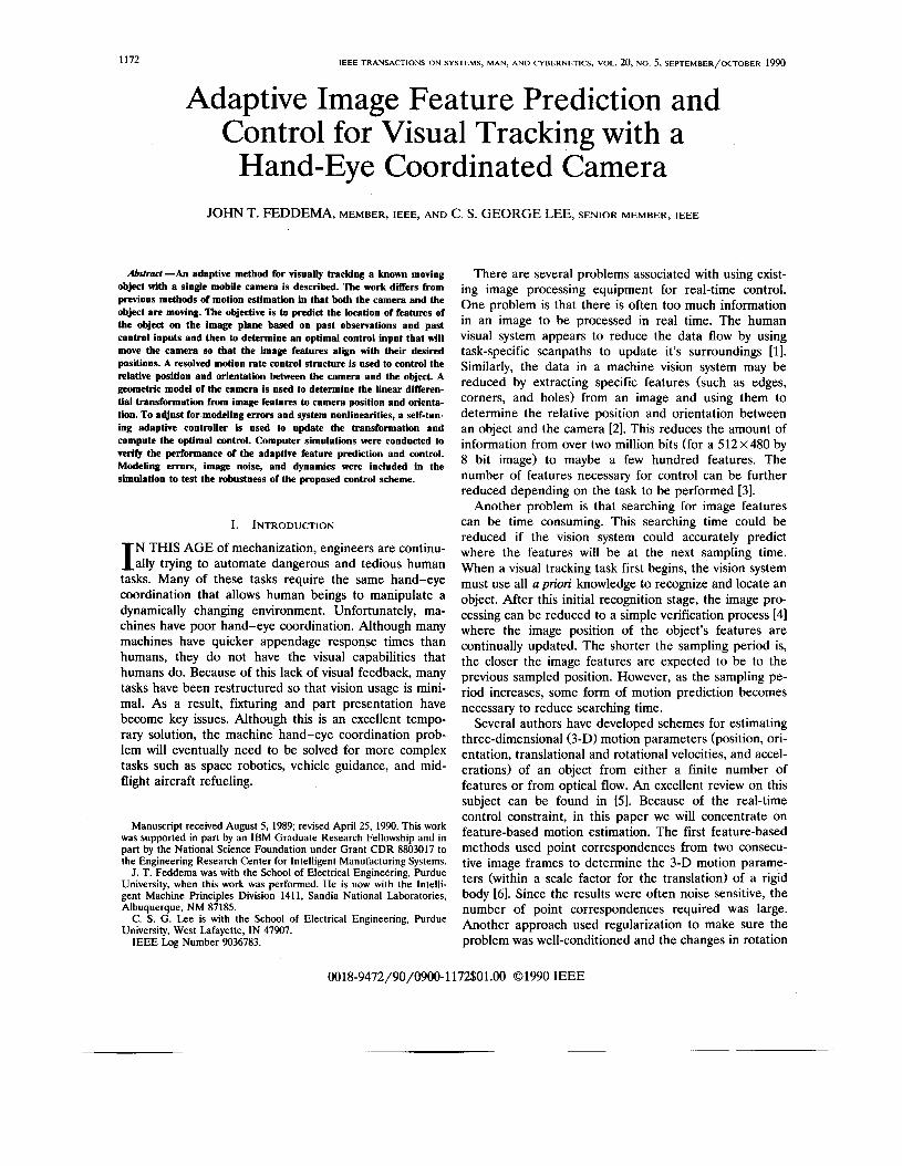
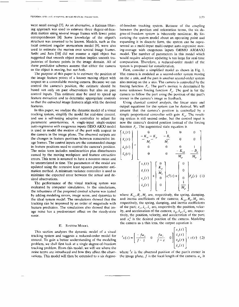
First, consider a simplified model as shown in Fig. 1. The camera is modeled as a second-order system moving on the x axis, and the part is another second-order system also moving on the x axis. The camera is controlled by the forcing function F,. The part’s motion is determined by some unknown forcing function F,,. The goal is for the camera to follow the part using the position of the part’s corner in the camera’s image as feedback.
Using classical control analysis, the linear state and output equations for the system can be derived. We will assume that the camera’s position is controlled by a simple proportional controller with gain K,. The result- ing system is still second order, but the control input is now the camera’s desired position instead of the forcing function F,. The augmented state equation is
where K , , , B,, M , are, respectively, the spring, damping, and inertia coefficients of the camera; K , / , , B,,, M , are, respectively, the spring, damping, and inertia coefficients of the part; x,, ic, x, are, respectively, the position, veloc- ity, and acceleration of the camera; x p , i/,, xp are, respec- tively, the position, velocity, and acceleration of the part; and x,“ is the desired position of the camera. Modeling the camera as a thin lens, the output equation is
where ‘x is the observed position of the part’s corner in the image plane, f is the focal length of the camera, a, is
1174 IEEE TRANSACTIONS ON SYSTEMS, MAN, AND CYBERNETICS, VOL. 20, NO. 5, SEPTEMBER/OCTOBER 1990
I X X X
C
Fig. 1 . One-dimensiqnal model for visual feedback system.
the scaling factor resulting from the camera sampling, z is the constant height between the camera and the part's corner, and c is the noise associated with the obser- vation ' x .
Assuming uniform sampling with period T and using Euler's method to approximate the derivatives, the system in (1) and (2) can be written in discrete form as
and F , r, G , and H are constant matrices similar to those in (1) and (2) but also a function of the sampling period T. If the dynamic parameters (mass, damping coefficient, and spring constant) for both the camera and the work- piece were known, it would be appropriate to use a Kalman filtering approach [8] to control the system. How- ever, in most real situations, the dynamics of both the part and the camera will probably not be known. As an alternative, we could express the system in terms of an ARMAX model and use an adaptive control technique to recursively update parameter estimates.
The state equation in (3) may be written in terms of the last n states and control inputs as
x ( k + n ) = ~ " x ( k ) + n
r l [ r u ( k + n - i ) r = l
+ G i ( k + n - i ) ] . ( 5 )
Assuming that the matrix F has a characteristic polyno-
mial
p ( A ) = A" + ulA"-' + * * + U , , n = 4, (6) and using the Cayley-Hamilton theorem, we can show that [ 111
n
y ( k + n ) = - u , y ( k + n - j ) J = 1
n - 1 J
+ U,,-, C ~ ~ ' - I r u ( k + j - i ) I - 1 l = l
n
+ m - T u ( k + n - i ) r = l
n - 1 J
+ U , - , H F ' - ' G ~ ( k + j - i) j = 1 j = l
n + HF'%l(k + n - i) + u ( k + n )
+ C u , u ( k + n - j ) . (7)
1 = 1
n
r = l
The ARMAX model for the previous system may be written as
A( Z - ' > Y ( k ) = B( .-')U( k ) + C( z - ' ) ~ ( k ) (8) where
A( 2-1) = 1 + u 1 z - I + - * * + u, z - , ,
C ( 2-1) = C ' z - 1 + - * * + C n Z P ,
B( Z - ' ) = b,z-' + * * * + b,z-",
z- ' is the delay operator, and q(k) is the noise term. Since the parameters of this model are constants, a self- tuning adaptive controller [12], [131 could be used to adjust the parameter estimates and determine the optimal control. Since n = 4, the number of parameters which needs to be adaptively updated in this equation is 12.
Notice that in (8) the noise term ~ ( k ) is a combination of state noise l ( k ) and observation noise u(k) . Because of the nature of the observation noise term, u ( k ) may be assumed to have zero mean and be uncorrelated. How- ever, the forcing function ( 5 = F,) that moves the part will most likely have nonzero mean and be correlated over time. Therefore, the noise term ~ ( k ) will have nonzero mean and be correlated. One way of dealing with this colored noise term is to model it as another ARMA process driven by white noise [14]. Combining the two models results in a new ARMAX model driven by white noise. The parameters of the original two models would not be recoverable, but the adaptive control technique could still be applied.
Next, let us expand the model for a six degree-of-free- dom visual-tracking system. This problem is much more difficult since the dynamic equations of the camera and the workpiece and the thin lens perspective transforma- tion of the camera are all nonlinear. Consider the visual
FEDDEMA A N D LEE: ADAPTIVE IMAGE FEATURE PREDICTION 1175
feedback control system in Fig. 2. The dynamics of the camera may be represented as
%(t> = f,(x,(t),u(t)) (9) where x , ( t )E R6 is the camera’s pose (position and ori- entation) with respect to some fixed coordinate frame, u ( t ) E R6 is the control input, and f l is a nonlinear function. In the case of the camera being on the robot’s end-effector, the nonlinear function f represents the robot’s dynamics [15]. Similarly, the workpiece’s dynamics may be represented by
.iPW = f,(.,(t),s(t>) ( 10)
where x, ( t )E R6 is the workpiece’s pose with respect to the fixed coordinate frame, [ ( t ) E R6 is the disturbance moving the workpiece, and f2 is a nonlinear function.
At this point, we are going to assume that the motion of the camera and the workpiece are slow enough that we can approximate the system as linear about an operating point and neglect higher order terms. Within the realms of realizable equipment, this is a fairly good assumption because of the rather slow image processing time (greater than 30 milliseconds) of most vision equipment. The sam- pling time of the image processing equipment and the field of view of the camera will constrain the tracking ability of the system. Linearizing about operating points (xc, U ) , and (x,, 5l0, (9) and (101, respectively, become
A i c ( t ) = F , A x , ( t ) + r , A u ( t ) (11)
A i P ( t ) = F2 Ax , ( t ) + G2 A [ ( f ) (12) and
where
Discretizing and using a Euler approximation for the derivatives, the augmented state equation is
A x , ( k + l ) Z + F I T [ A x P ( k + l ) ] = [ 0
or
A x ( k + 1) = F A x ( k ) + T A u ( k ) + G A L ( k ) (14) where T is the sampling period, Z is a 6 x 6 identity matrix, and 0 is a 6 X 6 zero matrix.
Similar to the one-dimensional (1-D) example, the ob- servation equation may be represented by geometric op- tics. The transformation from a point in three-dimen- sional (3-D) space to the two-dimensional (2-D) image plane can be modeled by a thin lens perspective transfor-
mation followed by the camera’s sampling:
cyx 0 0 x o [;;I=[ 0 f f y 0 Y o 0 0 0 1
or
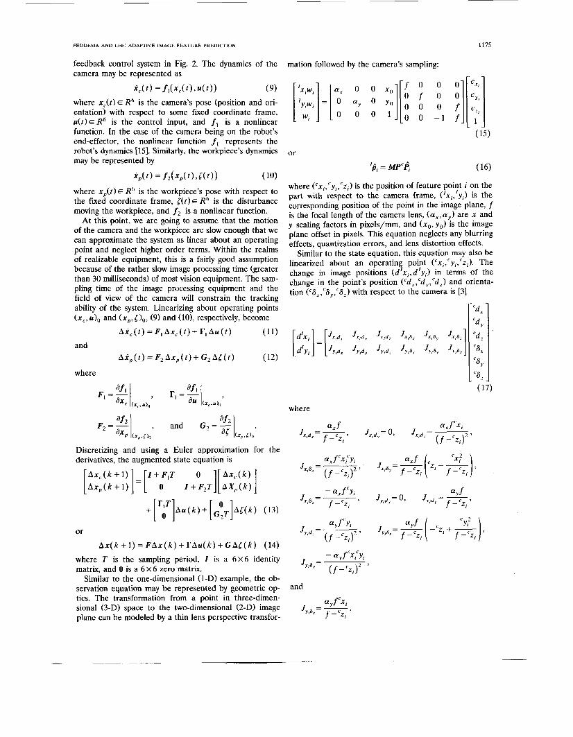
where (cx,,cy,,cz,) is the position of feature point i on the part with respect to the camera frame, (‘x,,’y,) is the corresponding position of the point in the image plane, f is the focal length of the camera lens, (a , ,ay) are x and y scaling factors in pixels/mm, and ( x o , y o ) is the image plane offset in pixels. This equation neglects any blurring effects, quantization errors, and lens distortion effects.
Similar to the state equation, this equation may also be linearized about an operating point (cx,,cy,,cz,). The change in image positions (d’x,,d‘y,) in terms of the change in the point’s position (cdx,cdy,cdz) and orienta- tion (c6x,c6y,‘6z) with respect to the camera is [3]
d’x
d’yi
where
and
1176 IEEE TRANSACTIONS ON SYSTEMS, MAN, AND CYBERNETICS, VOL. 20, NO. 5, SEPTEMBER/OCTOBER 1990
For M points, this Jacobian relationship may be written as
A'y = Qc A'x, (18)
where A'y E R 2 M is ,the change in position in the image plane, and Acxc E R6 is the instantaneous change in cam- era pose with respect to the camera frame.
In order for (18) to be the observation equation, Acxc must be expressed in terms of the state A x = [Ax,TAx,TIT. The relationship between a point expressed in terms of a fixed coordinate frame ( x , y , z ) and the same point ex- pressed in terms of the camera's coordinate frame (cx, ' y , 'z) is represented by the homogeneous transforma- tion [15]
or
r; = Tee$ ( 20) where n, 0, and U are the orientation vectors, and p is the position vector of the camera with respect to the fixed frame. The Jacobian relationship between changes in pose with respect to the fixed frame and changes in pose with respect to the camera's frame is [15]
AX = JcAcx (21)
or
where
R c = [ n o U ] ,
and
S , = [ ( p X n ) ( P X O ) ( P X 4 1 .
Assuming the changes in pose are small, the relative change in pose with respect to the camera can be approxi- mated as the difference between the changes caused by moving the camera Acxc and changes caused by moving the part Acxp. Combining (18) and (211, the observation equation can be written as
A'y( k ) = H A x ( k ) +'v( k ) (23) where
H = [ -3 J - 1 kcJ;l] E R 2 M x 1 2 (24)
and 'v(k) E R2M is white noise associated with the obser- vations.
Using the Cayley-Hamilton theorem, we can show that the state and observation equations in (14) and (23) can be combined to form a MIMO ARMAX model of the
form [ l l ]
A( z - I ) [ A'y( k ) --'U( k ) ]
= [ B( 2-')I Au( k ) + [ C( Z - ' ) I A l ( k ) (25) where
A( z - ' ) = 1 + a,z-' + * - * + u , ~ z - ' ~ E RI,
[ B( 2-')I = B,z-' + . . . + B 12 2 - l ' E R 2 M x 6 ,
and [ C( Z-I)] = C,Z-' + . * * + C,,z-I2 E R 2 M x 6 .
The number of parameters that would need to be adap- tively updated in (25) is 12 + 288 x M.
For our purposes, adaptively updating this many pa- rameters is impractical. In addition, the set of parameters which fit a particular set of data is not unique. The initial parameter estimates must be fairly accurate in order for a recursive algorithm to correctly converge to the appropri- ate system model. Since a system's real-time computing power is often limited and it is difficult to determine initial parameter estimates, we have reduced the model to the linear system
A'y( k ) = B , Au( k - d ) + q( k ) (26)
Bl = - k c J J 1 r , T , (27)
where
q ( k ) includes all the other terms, and d is an integer greater than or equal to one, representing the system delay time. The number of parameters is reduced to 12x M.
As shown in (171, if we know approximately where the positions of the feature points are with respect to the camera, we can determine an expression for 'J,. This matrix will have an exact inverse if the feature points are chosen to be three noncollinear points in the image [16], [17]. It is also possible to determine a close approximation of the differential transformation from the camera coordi- nates to the control coordinates, Jc- ' r1 , from the kine- matics of the camera controller [161, [171. It has been shown [3], [16], [17] that reasonable tracking results can be obtained using the inverse of the modeled transformation B , and neglecting the noise term q. However, these results deteriorate if the modeled transformations are not accurate; for example, if the x and y scaling factors in (17) are not precise. In addition, these linear transforma- tions are only valid about an operating point. The track- ing errors increase as the actual feature points move away from points ( c x l , c y l , c z I ) used to compute (17). Therefore, the tracking results could be improved and made more robust if B , could be adaptively updated.
The ideal transformation from the feature space to the control space may be expressed as a product of the modeled transformations, B,, =Qc, J;LI'lmT, and a ma- trix @ E R 2 M x 2 M representing the modeling errors:
B , = - 0 Qc, .I:; r l m T . (28)
FEDDEMA A N D LEE: ADAPTIVE IMAGE FEATURE PREDICTION 1177
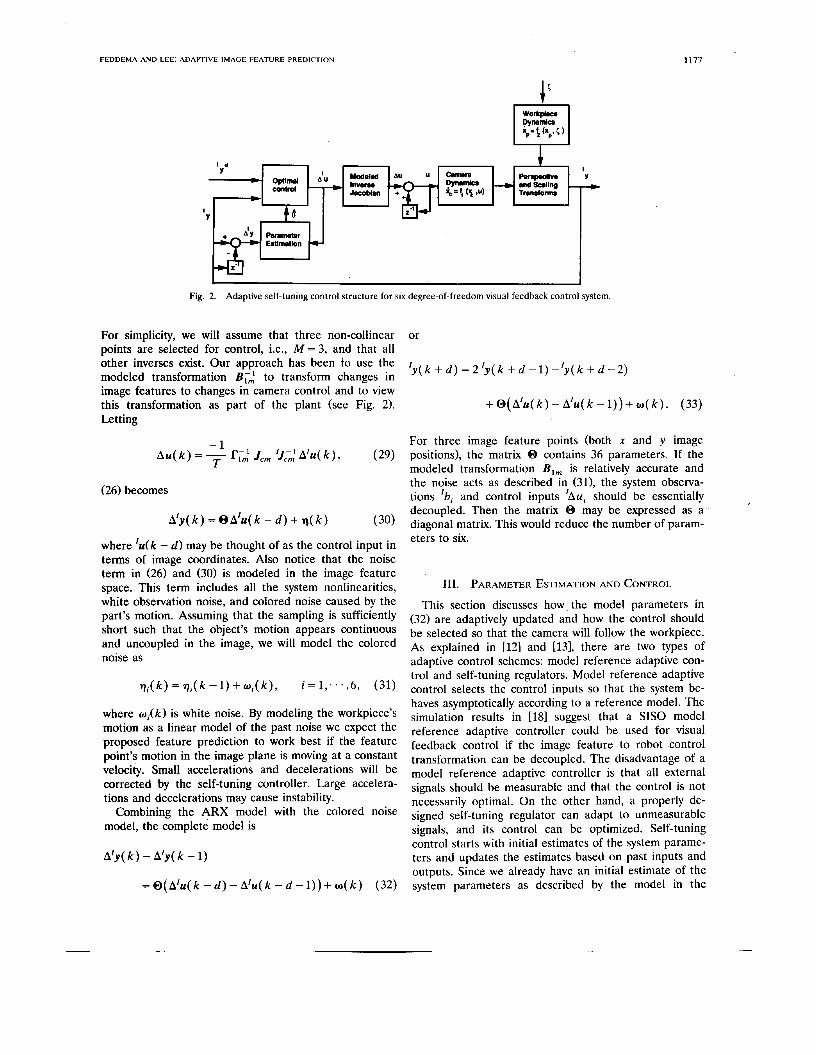
Fig. 2. Adaptive self-tuning control structure for six degree-of-freedom visual feedback control system.
For simplicity, we will assume that three non-collinear points are selected for control, i.e., M = 3, and that all other inverses exist. Our approach has been to use the modeled transformation B ; , to transform changes in image features to changes in camera control and to view this transformation as part of the plant (see Fig. 2). Letting
- 1
(26) becomes
A’y( k ) = @A’u( k - d ) + q( k ) ( 30)
where ’u(k - d ) may be thought of as the control input in terms of image coordinates. Also notice that the noise term in (26) and (30) is modeled in the image feature space. This term includes all the system nonlinearities, white observation noise, and colored noise caused by the part’s motion. Assuming that the sampling is sufficiently short such that the object’s motion appears continuous and uncoupled in the image, we will model the colored noise as
~ ; ( k ) = qi( k - 1) + w;( k ) , i = 1,. . . ,6, (31)
where o & k ) is white noise. By modeling the workpiece’s motion as a linear model of the past noise we expect the proposed feature prediction to work best if the feature point’s motion in the image plane is moving at a constant velocity. Small accelerations and decelerations will be corrected by the self-tuning controller. Large accelera- tions and decelerations may cause instability.
Combining the ARX model with the colored noise model, the complete model is
A ’ ~ ( k ) - A’Y( k - 1)
= @( A’u( k - d ) - A’u( k - d - 1)) + W( k ) (32)
or
’y( k + d ) = 2 ‘y( k + d - 1) -’y ( k + d - 2)
+ o( A’U( k ) - A’U( k - I ) ) + W( k ) . (33)
For three image feature points (both x and y image positions), the matrix 0 contains 36 parameters. If the modeled transformation B,, is relatively accurate and the noise acts as described in (311, the system observa- tions ‘b, and control inputs ’Au; should be essentially decoupled. Then the matrix 0 may be expressed as a diagonal matrix. This would reduce the number of param- eters to six.
I
111. PARAMETER ESTIMATION AND CONTROL
This section discusses how the model parameters in (32) are adaptively updated and how the control should be selected so that the camera will follow the workpiece. As explained in [12] and [13], there are two types of adaptive control schemes: model reference adaptive con- trol and self-tuning regulators. Model reference adaptive control selects the control inputs so that the system be- haves asymptotically according to a reference model. The simulation results in [18] suggest that a SISO model reference adaptive controller could be used for visual feedback control if the image feature to robot control transformation can be decoupled. The disadvantage of a model reference adaptive controller is that all external signals should be measurable and that the control is not necessarily optimal. On the other hand, a properly de- signed self-tuning regulator can adapt to unmeasurable signals, and its control can be optimized. Self-tuning control starts with initial estimates of the system parame- ters and updates the estimates based on past inputs and outputs. Since we already have an initial estimate of the system parameters as described by the model in the
1178 IEEE TRANSACTIONS ON SYSTEMS, MAN, A N D CYBERNETICS, VOL. 20, NO. 5, SEPTEMBER/OCTOBER 1990
I - - - - - - 1
Jacoblan
Part’s Location In World Coord.
1
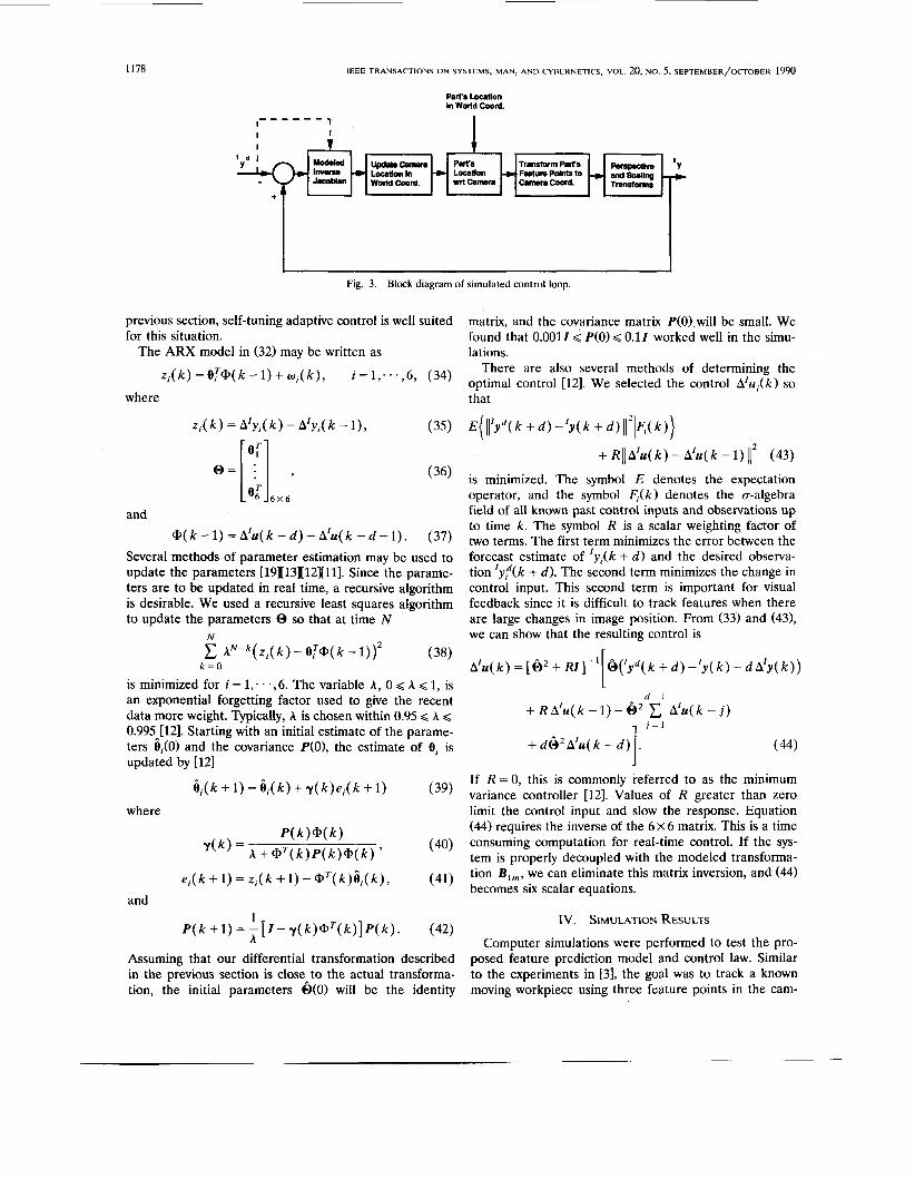
I I Block diagram of simulated control loop. Fig. 3.
previous section, self-tuning adaptive control is well suited for this situation.
The ARX model in (32) may be written as
z i ( k ) = fJT@(k - 1) + w i ( k ) , i = 1;. * , 6 , (34)
where
zi( k ) = A’Y,( k ) - b’yi( k - I ) , (35) @=[;I 3 (36)
6 x 6
and @( k - 1) = A’U( k - d ) - A’U( k - d - 1) . (37)
Several methods of parameter estimation may be used to update the parameters [191[13][121[11]. Since the parame- ters are to be updated in real time, a recursive algorithm is desirable. We used a recursive least squares algorithm to update the parameters 8 so that at time N
N
A ~ - ~ ( Z ~ ( ~ ) - - ~ J T @ ( ~ -I))* (38) k = O
is minimized for i = 1; . - ,6 . The variable A , 0 G A G 1, is an exponential forgetting factor used to give the recent data more weight. Typically, A is chosen within 0.95 G A G 0.995A[12]. Starting with an initial estimate of the parame- ters O,(O) and the covariance P(O), the estimate of fJi is updated by [121
i i ( k + 1) = i i ( k ) + y ( k ) e , ( k + 1) (39) where
e;( k + 1) = zi( k + 1) - aT( k ) i i ( k ) , (41) and
1 A
P( k + 1) = -[ Z - y ( k ) Q T ( k ) ] P ( k ) . (42)
Assuming that our differential transformation described in the previous section is close-to the actual transforma- tion, the initial parameters @(O) will be the identity
matrix, and the covariance matrix P(0) will be small. We found that 0.0011 G P(0) G 0.11 worked well in the simu- lations.
There are also several methods of determining the optimal control [121. We selected the control A’u,(k) so that
E( Il’Yd(k + 4 -‘Y(k + 4 I121F,(k))
+ R I I A ’ ~ ( ~ ) - A L ( ~ - 1) (43) is minimized. The symbol E denotes the expectation operator, and the symbol F,(k) denotes the a-algebra field of all known past control inputs and observations up to time k. The symbol R is a scalar weighting factor of two terms. The first term minimizes the error between the forecast estimate of ‘y , (k + d ) and the desired observa- tion ‘ y p ( k + d) . The second term minimizes the change in control input. This second term is important for visual feedback since it is difficult to track features when there are large changes in image position. From (33) and (431, we can show that the resulting control is
A‘@( k ) = [ d2 + RI] - ’ dryd( k + d ) -‘y ( k ) - d A’y ( k ) )
d - 1 [
+ R A ’ U ( ~ - I ) - & ~ ~ ‘ ~ ( k - j )
+ db2A‘u( k - d ) . (44) 1 If R = 0, this is commonly referred to as the minimum variance controller [12]. Values of R greater than zero limit the control input and slow the response. Equation (44) requires the inverse of the 6 X 6 matrix. This is a time consuming computation for real-time control. If the sys- tem is properly decoupled with the modeled transforma- tion B,, , we can eliminate this matrix inversion, and (44) becomes six scalar equations.
IV. SIMULATION RESULTS
Computer simulations were performed to test the pro- posed feature prediction model and control law. Similar to the experiments in [3], the goal was to track a known moving workpiece using three feature points in the cam-
FEDDEMA AND LEE: ADAPTIVE IMAGE FEATURE PREDICTION 1179
Y 1 E
1 0 0 0 - 800 -
- 2 0 0 -
- 4 0 0 - 1
I I I I 0 5 0 1 0 0 1 5 0
samples
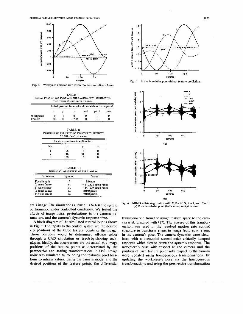
Fig. 4. Workpiece’s motion with respect to fixed coordinate frame.
TABLE I INITIAL POSE OF THE PART AND THE CAMERA WITH RESPECT TO
THE FIXED COORDINATE FRAME
Initial position (in mm) and orientation (in degrees)
X Y z roll pitch yaw Workpiece 0 0 0 0 0 0 Camera 50 50 -200 0 0 0
TABLE I1 POSITIONS OF THE FEATURE POINTS WITH RESPECT
Feature positions in millimeters
TO THE PART’S FRAME
No. X Y z
1 98 5 0 2 46 91 0 3 28 6 0
TABLE 111 INTRINSIC PARAMETERS OF THE CAMERA
Parameter SpbOl Value
8.0 mm - 67.2832 pixels/mm
Y scale factor f f Y - 84.7279 pixels/mm X focal center XI) 240.0 pixels Y focal center Y 0 240.0 pixels
Focal length f X scale factor f fx
era’s image. The simulations allowed us to test the system performance under controlled conditions. We tested the effects of image noise, perturbations in the camera pa- rameters, and the camera’s dynamic response time.
A block diagram of the simulated control loop is shown in Fig. 3. The inputs to the control system are the desired x , y positions of the three feature points in the image. These positions would be determined off-line either through a CAD simulation or teach-by-showing tech- niques. Ideally, the observations are the actual x , y image positions of the feature points as determined by the perspective and scaling transformations in (15). Image noise was simulated by rounding the features’ pixel loca- tions to integer values. Using the camera model and the desired positions of the feature points, the differential
- 3 P V
I
E
a?
B .g B - e E
L E
1 5
1 0
5
0
- 5
- 1 0
- 1 5
0 5 0 1 0 0 1 5 0 samples
Errors in relative pose without feature prediction. Fig. 5.
3 g U 6 E - H
:I - x Y
I011 Ditch
...._ . _ _
0
- 0
I I I
samples
- 1 0 5 0 1 0 0 1 5 0
(a)
4 4 ,
Y I I I 0 5 0 1 0 0 1 5 0
samples
(b) Fig. 6. MIMO self-tuning control with P(0) = O.I*I, A = 1, and R = Q.
(a) Error in relative pose. (b) Feature prediction error.
transformation from the image feature space to the cam- era is determined with (17). The inverse of this transfor- mation was used in the resolved motion rate control structure to transform errors in image features to errors in the camera’s pose. The camera dynamics were simu- lated with a decoupled second-order critically damped response which slowed down the system’s response. The workpiece’s pose with respect to the camera and the position of each feature point with respect to the camera were updated using homogeneous transformations. By updating the workpiece’s pose via the homogeneous transformations and using the perspective transformation
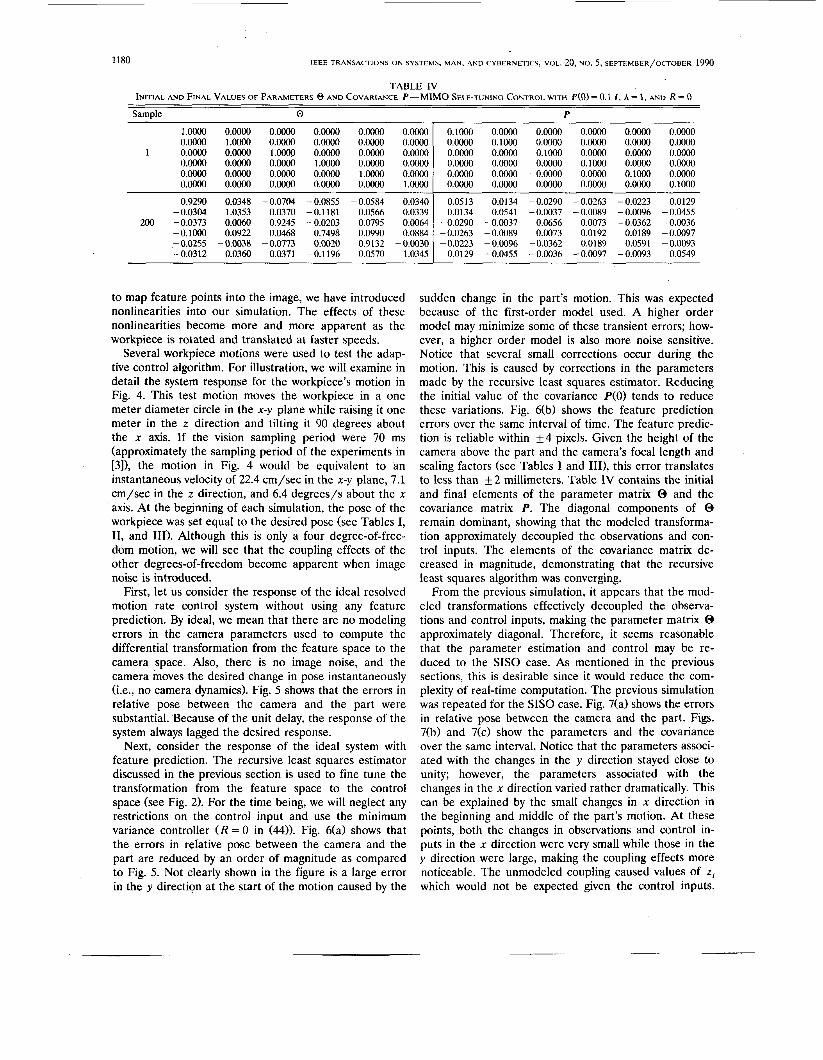
1180 IEEE TRANSACTIONS ON SYSTEMS, MAN, AND CYBERNETICS, VOL. 20, NO. 5, SEPTEMBER/OCTOBER 1990
TABLE IV INITIAL AND FINAL VALUES OF PARAMETERS @ AND COVARIANCE P-MIMO SELF-TUNING CONTROL WITH P(0) = 0.1 1, A = 1, A N D R = 0
Sample P
1.oOoo o.oo00 0.oOoo 1.oooo
1 0 . m 0 . m 0 . m o.oo00 0 . m o.oo00 0 . m 0 . m
0.0000 o.Ooo0 o.oo00 o.Ooo0 l.m o.oO0o o.oo00 l.m 0 . m 0 . m 0.0000 o.oo00
0.0000 O.oo00 O.oo00 O.oo00 1 .m O.oo00
O.oo00 O .oo00 0.0000 o.Ooo0 o.Ooo0 1 .m
0.9290 0.0348 - 0.0304 1.0353
200 -0.0373 0.0060 -0.loO0 0.0922 -0.0255 - 0.0038 -0.0312 0.0360
- 0.0704 - 0.0855 0.0370 -0.1181 0.9245 - 0.0203
- 0.0773 0.0020 0.0371 -0.1196
0.0468 0.7498
- 0.0584 0.0566
- 0.0795 0.0990 0.9132 0.0570
0.0340 0.0339 0.0064 0.0884
1.0345 - 0.0030
-
0.1000 0.0000 0.0000 0.0000 0.0000 0.oOoo
0.0000 0.1000 0.0000 0.0000 0.0000 0.0000
0.0000 0 . m 0.0000 0.0000 0.1000 0 . m 0.0000 0.1Ooo 0.0000 o.Ooo0 0.0000 0.0000
O.oo00 O.oo00 O .oo00 o.Ooo0 0.1Ooo O.oo00
0.0000 O.oo00 0.0000 0.0000 O.oo00 0.1000
0.0513 0.0134
- 0.0290 - 0.0263 - 0.0223
0.0129
0.0134 0.0541
- 0.0037 - 0.0089 - 0.0096 - 0.0455
- 0.0290 - 0.0263 - 0.0037 - 0.0089
0.0656 0.0073 0.0073 0.0192
- 0.0362 0.0189 - 0.0036 - 0.0097
- 0.0223 - 0.0096 - 0.0362
0.0189 0.0591
- 0.0093
0.0129 - 0.0455 - 0.0036 - 0.0097 - 0.0093
0.0549
to map feature points into the image, we have introduced nonlinearities into our simulation. The effects of these nonlinearities become more and more apparent as the workpiece is rotated and translated at faster speeds.
Several workpiece motions were used to test the adap- tive control algorithm. For illustration, we will examine in detail the system response for the workpiece’s motion in Fig. 4. This test motion moves the workpiece in a one meter diameter circle in the x-y plane while raising it one meter in the z direction and tilting it 90 degrees about the x axis. If the vision sampling period were 70 ms (approximately the sampling period of the experiments in [31), the motion in Fig. 4 would be equivalent to an instantaneous velocity of 22.4 cm/sec in the x-y plane, 7.1 cm/sec in the z direction, and 6.4 degrees/s about the x axis. At the beginning of each simulation, the pose of the workpiece was set equal to the desired pose (see Tables I, 11, and 111). Although this is only a four degree-of-free- dom motion, we will see that the coupling effects of the other degrees-of-freedom become apparent when image noise is introduced.
First, let us consider the response of the ideal resolved motion rate control system without using any feature prediction. By ideal, we mean that there are no modeling errors in the camera parameters used to compute the differential transformation from the feature space to the camera space. Also, there is no image noise, and the camera moves the desired change in pose instantaneously (i.e., no camera dynamics). Fig. 5 shows that the errors in relative pose between the camera and the part were substantial. Because of the unit delay, the response of the system always lagged the desired response.
Next, consider the response of the ideal system with feature prediction. The recursive least squares estimator discussed in the previous section is used to fine tune the transformation from the feature space to the control space (see Fig. 2). For the time being, we will neglect any restrictions on the control input and use the minimum variance controller ( R = 0 in (44)). Fig. 6(a) shows that the errors in relative pose between the camera and the part are reduced by an order of magnitude as compared to Fig. 5. Not clearly shown in the figure is a large error in the y direction at the start of the motion caused by the
sudden change in the part’s motion. This was expected because of the first-order model used. A higher order model may minimize some of these transient errors; how- ever, a higher order model is also more noise sensitive. Notice that several small corrections occur during the motion. This is caused by corrections in the parameters made by the recursive least squares estimator. Reducing the initial value of the covariance P(0) tends to reduce these variations. Fig. 6(b) shows the feature prediction errors over the same interval of time. The feature predic- tion is reliable within f 4 pixels. Given the height of the camera above the part and the camera’s focal length and scaling factors (see Tables I and 1111, this error translates to less than f 2 millimeters. Table IV contains the initial and final elements of the parameter matrix 0 and the covariance matrix P. The diagonal components of 0 remain dominant, showing that the modeled transforma- tion approximately decoupled the observations and con- trol inputs. The elements of the covariance matrix de- creased in magnitude, demonstrating that the recursive least squares algorithm was converging.
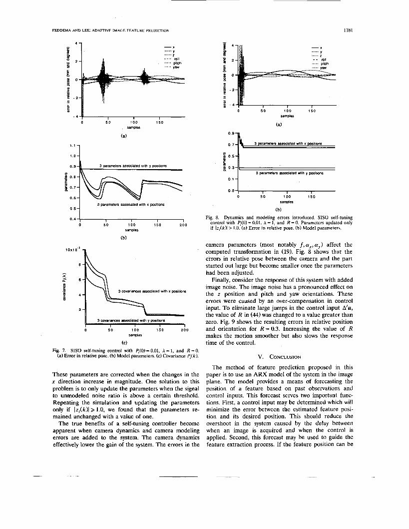
From the previous simulation, it appears that the mod- eled transformations effectively decoupled the observa- tions and control inputs, making the parameter matrix 0 approximately diagonal. Therefore, it seems reasonable that the parameter estimation and control may be re- duced to the SISO case. As mentioned in the previous sections, this is desirable since it would reduce the com- plexity of real-time computation. The previous simulation was repeated for the SISO case. Fig. 7(a) shows the errors in relative pose between the camera and the part. Figs. 7(b) and 7(c) show the parameters and the covariance over the same interval. Notice that the parameters associ- ated with the changes in the y direction stayed close to unity; however, the parameters associated with the changes in the x direction varied rather dramatically. This can be explained by the small changes in x direction in the beginning and middle of the part’s motion. At these points, both the changes in observations and control in- puts in the x direction were very small while those in the y direction were large, making the coupling effects more noticeable. The unmodeled coupling caused values of z, which would not be expected given the control inputs.
FEDDEMA A N D LEE: ADAPTIVE IMAGE FEATURE PREDICTION
U)
0 1 - g 0 8 - E g 0 7 -
0 0
1181
3 parameters associated with y positions
I I I I
b 4 1
- .......... ......
0 5 0 1 0 0 1 5 0 samples
- f
- 0 5 0 1 0 0 1 5 0 samples
(a)
Fig. 8. Dynamics and modeling errors introduced. SISO self-tuning control with P,(O) = 0.01, A = 1, and R = 0. Parameters updated only if Iz, (k)l> 1.0. (a) Error in relative pose. (b) Model parameters.
5 0 1 0 0 1 5 0 200 0 4 - 1
samples
(b) camera parameters (most notably f, ax, a,) affect the computed transformation in (19). Fig. 8 shows that the errors in relative pose between the camera and the part
10x1 o.3
8 started out large but become smaller once the parameters X had been adjusted. h e Finally, consider the response of this system with added
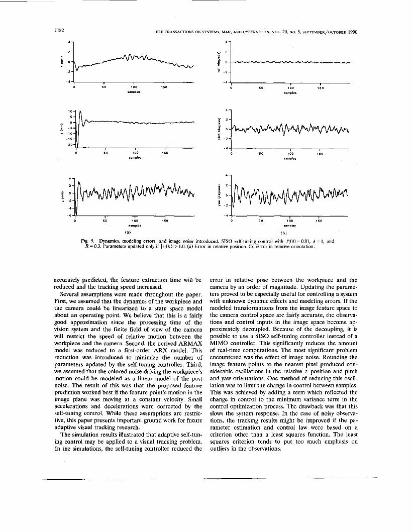
image noise. The image noise has a pronounced effect on the z position and pitch and yaw orientations. These errors were caused by an over-compensation in control
the value of R in (44) was changed to a value greater than zero. Fig. 9 shows the resulting errors in relative position
- 3 mvariances associated with x positions
E f 4 8
2 input. To eliminate large jumps in the control input A'u,
0 5 0 1 0 0 150 Z O O and orientation for R = 0 . 3 . Increasing the value of R samples
(C)
Fig. 7. SISO self-tuning control with F$O) = 0.01, A = 1, and R = 0. (a) Error in relative pose. (b) Model parameters. (c) Covariance Pi(k).
These parameters are corrected when the changes in the x direction increase in magnitude. One solution to this problem is to only update the parameters when the signal to unmodeled noise ratio is above a certain threshold. Repeating the simulation and updating the parameters only if Iz,(k)l> 1.0, we found that the parameters re- mained unchanged with a value of one.
The true benefits of a self-tuning controller becomz apparent when camera dynamics and camera modeling errors are added to the system. The camera dynamics effectively lower the gain of the system. The errors in the
makes the motion smoother but also slows the response time of the control.
V. CONCLUSION
The method of feature prediction proposed in this paper is to use an ARX model of the system in the image plane. The model provides a means of forecasting the position of a feature based on past observations and control inputs. This forecast serves two important func- tions. First, a control input may be determined which will minimize the error between the estimated feature posi- tion and its desired position. This should reduce the overshoot in the system caused by the delay between when an image is acquired and when the control is applied. Second, this forecast may be used to guide the feature extraction process. If the feature position can be
1182 IEEE TRANSACTIONS ON SYSTEMS, MAN, AND CYBERNETICS, VOL. 20, NO. 5, SEPTEMBER/OCTOBER 1990
4
2
E
0 - 2 i------ 5 0 samplss 1 0 0 1 5 0 iii - 4 5 0 samDles 1 0 0 1 5 0
- E O
- 2
- 4
- p 2 - i o B O
I B
a - 2
- 4
- 1 5
- 2 0
4 4
2
E O
N - 2
- 4
- 6 - 4
- - e 2 3 0 - E - 2
0 5 0 1 0 0 1 5 0 0 5 0 1 0 0 1 5 0 sa m p I e s sa m o I e s
(a) (b)
Fig. 9. Dynamics, modeling errors, and image noise introduced. SISO self-tuning control with P,(O) = 0.01, A = 1, and R = 0.3. Parameters updated only if Ir,(k)l> 1.0. (a) Error in relative position. (b) Error in relative orientation.
accurately predicted, the feature extraction time will be reduced and the tracking speed increased.
Several assumptions were made throughout the paper. First, we assumed that the dynamics of the workpiece and the camera could be linearized to a state space model about an operating point. We believe that this is a fairly good approximation since the processing time of the vision system and the finite field of view of the camera will restrict the speed of relative motion between the workpiece and the camera. Second, the derived ARMAX model was reduced to a first-order ARX model. This reduction was introduced to minimize the number of parameters updated by the self-tuning controller. Third, we assumed that the colored noise driving the workpiece's motion could be modeled as a linear model of the past noise. The result of this was that the proposed feature prediction worked best if the feature point's motion in the image plane was moving at a constant velocity. Small accelerations and decelerations were corrected by the self-tuning control. While these assumptions are restric- tive, this paper presents important ground work for future adaptive visual tracking research.
The simulation results illustrated that adaptive self-tun- ing control may be applied to a visual tracking problem. In the simulations, the self-tuning controller reduced the
error in relative pose between the workpiece and the camera by an order of magnitude. Updating the parame- ters proved to be especially useful for controlling a system with unknown dynamic effects and modeling errors. If the modeled transformations from the image feature space to the camera control space are fairly accurate, the observa- tions and control inputs in the image space become ap- proximately decoupled. Because of the decoupling, it is possible to use a SISO self-tuning controller instead of a MIMO controller. This significantly reduces the amount of real-time computations. The most significant problem encountered was the effect of image noise. Rounding the image feature points to the nearest pixel produced con- siderable oscillations in the relative z position and pitch and yaw orientations. One method of reducing this oscil- lation was to limit the change in control between samples. This was achieved by adding a term which reflected the change in control to the minimum variance term in the control optimization process. The drawback was that this slows the system response. In the case of noisy observa- tions, the tracking results might be improved if the pa- rameter estimation and control law were based on a criterion other than a least squares function. The least squares criterion tends to put too much emphasis on outliers in the observations.
FEDDEMA AND LEE: ADAPTJVE IMAGE FEATURE PREDJCTION 1183
REFERENCES [181 L. E. Weiss, A. C. Sanderson, and C. P. Neuman, “Dynamic sensor-based control of robots with visual feedback,” IEEE J.
R. Isermann, “Practical aspects of process identification,” Auto- matica, vol. 16, pp. 575-587, 1980.
L. W. Stark and S. R. Ellis, “Scanpaths revisited: Cognitive models direct active looking,” in ,rye M ~ ~ ~ ~ ~ ~ ~ ~ : cosnition and vuual Perception, D. F. Fisher, R. A. Monty, and J. W. Senders, Eds. Hillsdale, NJ: Lawrence Erlbaum Assoc., 1981. R. C. Bolles and R. A. Cain, “Recognizing and locating partially visible objects: The local-feature-focus method,” Int. J. Robotics Res., vol. 1 , no. 3, pp. 57-82, Fall 1982. J. T. Feddema, C. S. G. Lee, and 0. R. Mitchell, “Optimal selection of image features for resolved rate visual feedback con- trol,” Engineering Research Center Tech. Rep., TR-ERC 89-3, Schools of Engineering, Purdue Univ., West Lafayette, IN, Jan. 1989 (also accepted for publication in IEEE Trans. Robot. Automa.). R. C. Bolles, “Verification vision within a programmable assembly system,” Stanford AI Lab Memo AIM-275, 1975. J. K. Aggarwal and N. Nandhakumar, “On the computation of motion from sequences of images-A review,” Proc. IEEE, vol. 76, no. 8, Aug. 1988. R. Y. Tsai and T. S. Huang, “Uniqueness and estimation of three-dimensional motion parameters of rigid objects with curved surfaces,” IEEE Trans. Pattern Anal. Machine Intell., vol. PAMI-6, no. 1, pp. 13-27, Jan. 1984. Y. yasumoto and G. Medioni, “Robust estimation of three- dimensional motion parameters from a sequence of image frames using regularization,” IEEE Trans. Pattern Anal. Machine Intell., vol. PAMI-8, no. 4, pp. 464-471, July 1986. T. J. Broida and R. Chellappa, “Estimation of object motion parameters from noisy images,” IEEE Trans. Pattern Anal. Ma- chine Intell., vol. PAMI-8, no. l , pp. 90-99, Jan. 1986. J. Weng, T. S. Huang, and N. Ahuia, “3-D motion estimation,
RA-31 no. 5, pp. 404-417, Oct. 1987. [I91
John T. Feddema (S’86-M’86-S’87-M’89) re- ceived the B.S.E.E. degree from Iowa State University, Ames, in 1984 and the M.S.E.E. and the Ph.D. degrees from Purdue University, West Lafayette, IN, in 1986 and 1989, respectively. While completing the Ph.D. degree at Purdue, he was a research assistant for the Engineering Research Center for Intelligent Manufacturing Systems, working on visual feedback control for automated assembly.
Since September 1989, Dr. Feddema has been a Senior Member of Technical Staff at Sandia National Laboratories in Albuquerque, NM. He is working in the Intelligent Machine Principles Division on the control of flexible link manipulators and multisensor integration for real-time robotic control. Additional research interests include robotics, computer vision, sensor-based control, and computer integrated manufacturing.
Dr. Feddema is a member of Eta Kappa Nu and Tau Beta Pi.
understanding, and prediction from noisy image sequences,” IEEE Trans. Pattern Anal. Mach. Intell., vol. PAMI-9, no. 3, pp. 370-389, May 1987. I. K. Sethi and R. Jain, “Finding trajectories of feature points in a monocular image sequence,” IEEE Trans. Pattern Anal. Machine Intell., vol. PAMI-9, no. 1, pp. 56-73, Jan. 1987. G. C. Goodwin, P. J. Ramadge, and P. E. Caines, “Discrete time stochastic adaptive control,” SIAM J. Contr. and Optimization, vol. 19, no. 67, pp. 829-853, Nov. 1981. R. Isermann, “Parameter adaptive control algorithms-A tutorial,” Automatica, vol. 18, no. 5, pp. 513-528, 1982. K. J. Astrom and B. Wittenmark, Adaptive Control. Reading, MA. Addison-Wesley, 1989. B. D. 0. Anderson and J. B. Moore, Optimal Filtering. Engle- wood Cliffs, NJ: Prentice-Hall, pp. 288-292, 1979. R. P. Paul, Robot Manipulators: Mathematics, Programming, and Control. J. T. Feddema and 0. R. Mitchell, “Vision guided servoing with feature-based trajectory generation,” IEEE Trans. Robotics and Automation, vol. 5 , no. 5, pp. 691-700, Oct. 1989. J. T. Feddema, “Real-time visual feedback control for hand-eye coordinated robotic systems,” Ph.D. Thesis, School of Electrical Engineering, Purdue Univ., West Lafayette, IN 47907, Aug. 1989.
Cambridge, MA: MIT Press, 1981.
C. S. George Lee (S’71-S’78-M’78-SM’S6) re- ceived the B.S. and M.S. degrees in electrical engineering from Washington State University, Seattle, in 1973 and 1974, respectively, and the Ph.D. degree from Purdue University, West Lafayette, IN, in 1978.
In 1978-1985, he taught at Purdue University and the University of Michigan, Ann Arbor. Since 1985, he has been with the School of Electrical Engineering, Purdue University, where he is currently a Professor. His current
research interests include kinematics, dynamics and control, computa- tional algorithms and architectures for robot control, intelligent multi- robot assembly systems, and assembly planning.
Dr. Lee was an IEEE Computer Society Distinguished Visitor in 1983-1986, and the Organizer and Chairman of the 1988 NATO Ad- vanced Research Workshop on Sensor-Based Robots: Algorithms and Architectures. He is the Secretary of the IEEE Robotics and Automa- tion Society, a Technical Editor of the IEEE TRANSACTIONS ON ROBOTICS AND AUTOMATION, a co-author of Robotics: Control, Sensing, vision, and Intelligence, published by McGraw-Hill, and a co-editor of Tutorial on Robotics (second edition), published by IEEE Computer Society Press. He is a member of Sigma Xi and Tau Beta Pi.