arX

iv:1

407.

5055

v3 [

cs.C

V]

3 N

ov 2

014

1

Adaptive Image Denoising by Targeted DatabasesEnming Luo,Student Member, IEEE, Stanley H. Chan,Member, IEEE, and Truong Q. Nguyen,Fellow, IEEE

Abstract—We propose a data-dependent denoising procedureto restore noisy images. Different from existing denoisingalgo-rithms which search for patches from either the noisy imageor a generic database, the new algorithm finds patches froma database that contains relevant patches. We formulate thedenoising problem as an optimal filter design problem and maketwo contributions. First, we determine the basis function of thedenoising filter by solving a group sparsity minimization prob-lem. The optimization formulation generalizes existing denoisingalgorithms and offers systematic analysis of the performance.Improvement methods are proposed to enhance the patch searchprocess. Second, we determine the spectral coefficients of thedenoising filter by considering a localized Bayesian prior.Thelocalized prior leverages the similarity of the targeted database,alleviates the intensive Bayesian computation, and links the newmethod to the classical linear minimum mean squared errorestimation. We demonstrate applications of the proposed methodin a variety of scenarios, including text images, multiviewimagesand face images. Experimental results show the superiorityofthe new algorithm over existing methods.

Index Terms—Patch-based filtering, image denoising, externaldatabase, optimal filter, non-local means, BM3D, group sparsity,Bayesian estimation

I. I NTRODUCTION

A. Patch-based Denoising

Image denoising is a classical signal recovery problemwhere the goal is to restore a clean image from its observa-tions. Although image denoising has been studied for decades,the problem remains a fundamental one as it is the test bedfor a variety of image processing tasks.

Among the numerous contributions in image denoising inthe literature, the most highly-regarded class of methods,todate, is the class ofpatch-based image denoisingalgorithms[1–9]. The idea of a patch-based denoising algorithm issimple: Given a

√d×

√d patchq ∈ R

d from the noisy image,the algorithm finds a set of reference patchesp1, . . . ,pk ∈ R

d

and applies some linear (or non-linear) functionΦ to obtainan estimatep of the unknown clean patchp as

p = Φ(q; p1, . . . ,pk). (1)

For example, in non-local means (NLM) [1],Φ is a weightedaverage of the reference patches, whereas in BM3D [3],Φ isa transform-shrinkage operation.

E. Luo and T. Nguyen are with Department of Electrical and ComputerEngineering, University of California at San Diego, La Jolla, CA 92093,USA. Emails: eluo@ucsd.edu and nguyent@ece.ucsd.edu

S. Chan is with School of Electrical and Computer Engineering, PurdueUniversity, West Lafayette, IN 47907, USA. Email: stanleychan@purdue.edu

This work was supported in part by a Croucher Foundation Post-doctoralResearch Fellowship, and in part by the National Science Foundation undergrant CCF-1065305. Preliminary material in this paper was presented atthe 39th IEEE International Conference on Acoustics, Speech and SignalProcessing (ICASSP), Florence, May 2014.

B. Internal vs External Denoising

For any patch-based denoising algorithm, the denoisingperformance is intimately related to the reference patchesp1, . . . ,pk. Typically, there are two sources of these patches:the noisy image itself and an external database of patches.The former is known asinternal denoising[10], whereas thelatter is known asexternal denoising[11, 12].

Internal denoising is practically more popular than exter-nal denoising because it is computationally less expensive.Moreover, internal denoising does not require a training stage,hence making it free of training bias. Furthermore, Glasneret al. [13] showed that patches tend to recur within animage,e.g., at a different location, orientation, or scale. Thussearching for patches in the noisy image is often a plausibleapproach. However, on the downside, internal denoising oftenfails for rare patches — patches that seldom recur in an image.This phenomenon is known as “rare patch effect”, and iswidely regarded as a bottleneck of internal denoising [14,15]. There are some works [16, 17] attempting to alleviatethe rare patch problem. However, the extent to which thesemethods can achieve is still limited.

External denoising [6, 18–21] is an alternative solutionto internal denoising. Levin et al. [15, 22] showed that inthe limit, the theoretical minimum mean squared error ofdenoising is achievable using an infinitely large externaldatabase. Recently, Chan et al. [20, 21] developed a compu-tationally efficient sampling scheme to reduce the complexityand demonstrated practical usage of large databases. However,in most of the recent works on external denoising,e.g., [6, 18,19], the databases used aregeneric. These databases, althoughlarge in volume, do not necessarily contain useful informationto denoise the noisy image of interest. For example, it is clearthat a database of natural images is not helpful to denoise anoisy portrait image.

C. Adaptive Image Denoising

In this paper, we propose an adaptive image denoisingalgorithm using atargeted external database instead of agenericdatabase. Here, a targeted database refers to a databasethat contains imagesrelevantto the noisy image only. As willbe illustrated in later parts of this paper, targeted externaldatabases could be obtained in many practical scenarios, suchas text images (e.g., newspapers and documents), human faces(under certain conditions), and images captured by multiviewcamera systems. Other possible scenarios include images oflicense plates, medical CT and MRI images, and images oflandmarks.

The concept of using targeted external databases has beenproposed in various occasions,e.g., [23–28]. However, none

2

of these methods are tailored for image denoising problems.The objective of this paper is to bridge the gap by addressingthe following question:

(Q): Suppose we aregivena targeted external database, howshould we design a denoising algorithm which can

maximallyutilize the database?

Here, we assume that the reference patchesp1, . . . ,pk aregiven. We emphasize that this assumption is applicationspecific — for the examples we mentioned earlier (e.g., text,multiview, face, etc), the assumption is typically true becausethese images have relatively less variety in content.

When the reference patches are given, question (Q) maylook trivial at the first glance because we can extend existinginternal denoising algorithms in a brute-force way to handleexternal databases. For example, one can modify existing al-gorithms,e.g., [1, 3, 5, 29, 30], so that the patches are searchedfrom a database instead of the noisy image. Likewise, onecan also treat an external database as a “video” and feedthe data to multi-image denoising algorithms,e.g., [31–34].However, the problem of these approaches is that the bruteforce modifications are heuristic. There is no theoretical guar-antee of performance. This suggests that a straight-forwardmodification of existing methods doesnot solve question (Q),as the database is not maximally utilized.

An alternative response to question (Q) is to train a statis-tical prior of the targeted database,e.g., [6, 18, 19, 35–38].The merit of this approach is that the performance often hastheoretical guarantee because the denoising problem can nowbe formulated as a maximum a posteriori (MAP) estimation.However, the drawback is that many of these methods requirea large number of training samples which is not alwaysavailable in practice.

D. Contributions and Organization

In view of the above seemingly easy yet challenging ques-tion, we introduced a new denoising algorithm using targetedexternal databases in [39]. Compared to existing methods, themethod proposed in [39] achieves better performance and onlyrequires a small number of external images. In this paper, weextend [39] by offering the following new contributions:

1) Generalization of Existing Methods. We propose ageneralized framework which encapsulates a number ofdenoising algorithms. In particular, we show (in SectionIII-B) that the proposed group sparsity minimizationgeneralizes both fixed basis and PCA methods. Wealso show (in Section IV-B) that the proposed localBayesian MSE solution is a generalization of manyspectral operations in existing methods.

2) Improvement Strategies. We propose two improvementstrategies for the generalized denoising framework. InSection III-D, we present a patch selection optimizationto improve the patch search process. In Section IV-D,we present a soft-thresholding and a hard-thresholdingmethod to improve the spectral coefficients learned bythe algorithm.

3) Detailed Proofs. Proofs of the results in this paper and[39] are presented in the Appendix.

The rest of the paper is organized as follows. After outliningthe design framework in Section II, we present the abovecontributions in Section III – IV. Experimental results arediscussed in Section V, and concluding remarks are given inSection VI.

II. OPTIMAL L INEAR DENOISING FILTER

The foundation of our proposed method is the classicaloptimal linear denoising filter design problem [40]. In thissection, we give a brief review of the design framework andhighlight its limitations.

A. Optimal Filter

The design of an optimal denoising filter can be posed asfollows: Given a noisy patchq ∈ R

d, and assuming thatthe noise is i.i.d. Gaussian with zero mean and varianceσ2,we want to find a linear operatorA ∈ R

d×d such that theestimatep = Aq has the minimum mean squared error (MSE)compared to the ground truthp ∈ R

d. That is, we want tosolve the optimization

A = argminA

E[‖Aq − p‖22

]. (2)

Here, we assume thatA is symmetric, or otherwise theSinkhorn-Knopp iteration [41] can be used to symmetrizeA, provided that entries ofA are non-negative. Given asymmetricA, one can apply the eigen-decomposition,A =UΛUT , where U = [u1, . . . ,ud] ∈ R

d×d is the basismatrix andΛ = diag {λ1, . . . , λd} ∈ R

d×d is the diagonalmatrix containing the spectral coefficients. WithU and Λ,the optimization problem in (2) becomes

(U ,Λ) = argminU ,Λ

E

[∥∥∥UΛUTq − p∥∥∥2

2

], (3)

subject to the constraint thatU is an orthonormal matrix.The joint optimization (3) can be solved by noting the

following Lemma.Lemma 1:Let ui be theith column of the matrixU , and

λi be the(i, i)th entry of the diagonal matrixΛ. If q = p+η,

whereηiid∼ N (0, σ2I), then

E

[∥∥∥UΛUT q − p∥∥∥2

2

]=

d∑

i=1

[(1 − λi)

2(uTi p)

2 + σ2λ2i

].

(4)The proof of Lemma 1 is given in [42]. With Lemma 1,

the denoised patch as a consequence of (3) is as follows.Lemma 2:The denoised patchp using the optimalU and

Λ of (3) is

p = U

(diag

{ ‖p‖2‖p‖2 + σ2

, 0, . . . , 0

})UT q,

whereU is any orthonormal matrix with the first columnu1 = p/‖p‖2.

Proof: See Appendix A.

3

Lemma 2 states that if hypothetically we are given theground truthp, the optimal denoising process is to first projectthe noisy observationq onto the subspace spanned byp, thenperform a Wiener shrinkage‖p‖2/(‖p‖2 + σ2), and finallyre-project the shrinkage coefficients to obtain the denoisedestimate. However, since in reality we never have access tothe ground truthp, this optimal result is not achievable.

B. Problem Statement

Since the oracle optimal filter is not achievable in practice,the question becomes whether it is possible to find a surrogatesolution that does not require the ground truthp.

To answer this question, it is helpful to separate the jointoptimization (3) by first fixingU and minimize the MSE withrespect toΛ. In this case, one can show that (4) achieves theminimum when

λi =(uT

i p)2

(uTi p)

2 + σ2, (5)

in which the minimum MSE estimator is given by

p = U

(diag

{(uT

1 p)2

(uT1 p)

2 + σ2, . . . ,

(uTd p)

2

(uTd p)

2 + σ2

})UTq,

(6)where{u1, . . . ,ud} are the columns ofU .

Inspecting (6), we identify two parts of the problem:

1) DetermineU . The choice ofU plays a critical role inthe denoising performance. In literature,U are typicallychosen as the FFT or the DCT bases [3, 4]. In [5, 7, 8],the PCA bases of various data matrices are proposed.However, the optimality of these bases is not fullyunderstood.

2) DetermineΛ. Even if U is fixed, the optimalΛ in(5) still depends on the unknown ground truthp. In[3], Λ is determined by hard-thresholding a stack ofDCT coefficients or applying an empirical Wiener filterconstructed from a first-pass estimate. In [7],Λ isformed by the PCA coefficients of a set of relevantnoisy patches. Again, it is unclear which of these isoptimal.

Motivated by the problems aboutU andΛ, in the followingtwo sections we present our proposed method for each ofthese problems. We discuss its relationship to prior works,and present ways to further improve it.

III. D ETERMINEU

In this section, we present our proposed method to deter-mine the basis matrixU and show that it is a generalizationof a number of existing denoising algorithms. We also discussways to improveU .

A. Patch Selection viak Nearest Neighbors

Given a noisy patchq and a targeted database{pj}nj=1, ourfirst task is to fetch thek most “relevant” patches. The patch

selection is performed by measuring the similarity betweenq

and each of{pj}nj=1, defined as

d(q,pj) = ‖q − pj‖2, for j = 1, . . . , n. (7)

We note that (7) is equivalent to the standardk nearestneighbors (kNN) search.kNN has a drawback that under theℓ2 distance, some of the

k selected patches may not be truly relevant to the denoisingtask, because the query patchq is noisy. We will come back tothis issue in Section III-D by discussing methods to improvethe robustness of thekNN.

B. Group Sparsity

Without loss of generality, we assume that thekNN re-turned by the above procedure are the firstk patches of thedata, i.e.,{pj}kj=1. Our goal now is to constructU from{pj}kj=1.

We postulate that a goodU should have two properties.First, U should make the projected vectors{UTpj}kj=1

similar in both magnitude and location. This hypothesisfollows from the observation that since{pj}kj=1 have smallℓ2 distances fromq, it must hold that anypi andpj (henceUTpi andUTpj) in the set should also be similar. Second,we require that each projected vectorUTpj contains as fewnon-zeros as possible,i.e., sparse. The reason is related to theshrinkage step to be discussed in Section IV, because a vectorof few non-zero coefficients has higher energy concentrationand hence is more effective for denoising.

In order to satisfy these two criteria, we propose to considerthe idea ofgroup sparsity1, which is characterized by thematrix ℓ1,2 norm, defined as2

‖X‖1,2 def=

d∑

i=1

‖xi‖2, (8)

for any matrixX ∈ Rd×k, wherexi ∈ R

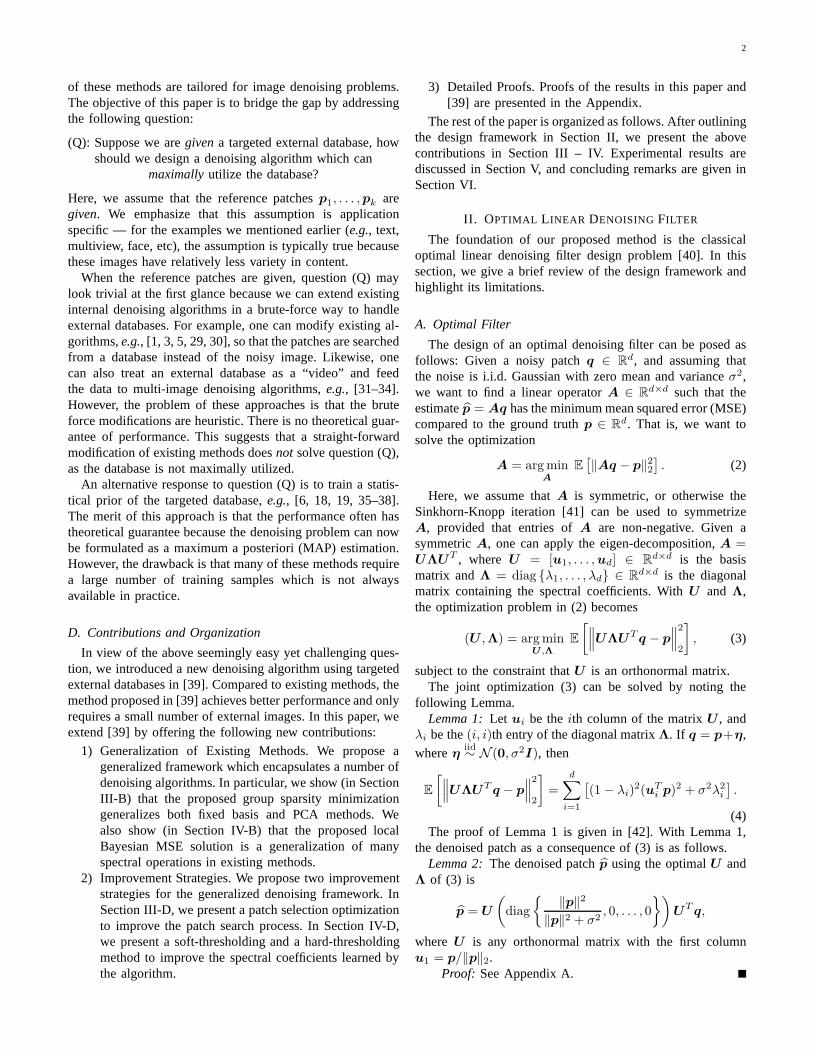
k is the ith row ofa matrixX. In words, a small‖X‖1,2 makes sure thatXhas few non-zero entries, and the non-zero entries are locatedsimilarly in each column [6, 43]. A pictorial illustration isshown in Figure 1.

Going back to our problem, we propose to minimize theℓ1,2-norm of the matrixUTP :

minimizeU

‖UTP ‖1,2subject to UTU = I,

(9)

where Pdef= [p1, . . . ,pk]. The equality constraint in (9)

ensures thatU is orthonormal. Thus, the solution of (9) is anorthonormal matrixU which maximizes the group sparsity ofthe dataP .

1Group sparsity was first proposed by Cotter et al. for group sparsereconstruction [43] and later used by Mairal et al. for denoising [6], buttowards a different end from the method presented in this paper.

2In general one can defineℓp,q norm as‖X‖p,q =∑d

i=1‖xi‖

pq , c.f.

[6].

4

(a) sparse (b) group sparse

Fig. 1: Comparison between sparsity (where columns aresparse, but do not coordinate) and group sparsity (where allcolumns are sparse with similar locations).

Interestingly, and surprisingly, the solution of (9) is indeedidentical to the classical principal component analysis (PCA).The following lemma summarizes the observation.

Lemma 3:The solution to (9) is that

[U ,S] = eig(PP T ), (10)

whereS is the corresponding eigenvalue matrix.Proof: See Appendix B.

Remark 1: In practice, it is possible to improve the fidelityof the data matrixP by introducing a diagonal weight matrix

W =1

Zdiag

{e−‖q−p

1‖2/h2

, . . . , e−‖q−pk‖2/h2}, (11)

for some user tunable parameterh and a normalizationconstantZ

def= 1

TW1. Consequently, we can define

P = PW 1/2. (12)

Hence (10) becomes[U ,S] = eig(PWP T ).

C. Relationship to Prior Works

The fact that (10) is the solution to a group sparsity mini-mization problem allows us to understand the performance ofa number of existing denoising algorithms to some extent.

1) BM3D [3]: It is perhaps a misconception that theunderlying principle of BM3D is to enforce sparsity of the3-dimensional data volume (which we shall call it a 3-waytensor). However, what BM3D enforces is thegroup sparsityof the slices of the tensor, not the sparsity of the tensor.

To see this, we note that the 3-dimensional transformsin BM3D are separable (e.g., DCT2 + Haar in its defaultsetting). If the patchesp1, . . . ,pk are sufficiently similar,the DCT2 coefficients will be similar inboth magnitude andlocation 3. Therefore, by fixing the frequency location of aDCT2 coefficient and tracing the DCT2 coefficients along thethird axis, the output signal will be almost flat. Hence, thefinal Haar transform will return a sparse vector. Clearly, suchsparsity is based on the stationarity of the DCT2 coefficientsalong the third axis. In essence, this is group sparsity.

3By DCT2 location we meant the frequency of the DCT2 components.

2) HOSVD [9]: The true tensor sparsity can only beutilized by the high order singular value decomposition(HOSVD), which is recently studied in [9]. LetP ∈R

√d×

√d×k be the tensor by stacking the patchesp1, . . . ,pk

into a 3-dimensional array, HOSVD seeks three orthonormalmatricesU (1) ∈ R

√d×

√d, U (2) ∈ R

√d×

√d, U (3) ∈ R

k×k

and an arrayS ∈ R

√d×

√d×k, such that

S = P ×1 U(1)T ×2 U

(2)T ×3 U(3)T ,

where×k denotes a tensor mode-k multiplication [44].As reported in [9], the performance of HOSVD is indeed

worse than BM3D. This phenomenon can now be explained,because HOSVD ignores the fact that image patches tend tobe group sparse instead of being tensor sparse.

3) Shape-adaptive BM3D [4]:As a variation of BM3D,SA-BM3D groups similar patches according to a shape-adaptive mask. Under our proposed framework, this shape-adaptive mask can be modeled as a spatial weight matrixW s ∈ R

d×d (where the subscripts denotesspatial). AddingW s to (12), we define

P = W 1/2s PW 1/2. (13)

Consequently, the PCA ofP is equivalent to SA-BM3D.Here, the matrixW s is used to control the relative emphasisof each pixel in the spatial coordinate.

4) BM3D-PCA [5] and LPG-PCA [7]: The idea of bothBM3D-PCA and LPG-PCA is that givenp1, . . . ,pk, U isdetermined as the principal components ofP = [p1, . . . ,pk].Incidentally, such approaches arrive at the same result as (10),i.e., the principal components are indeed the solution of agroup sparse minimization. However, the key of using thegroup sparsity is not noticed in [5] and [7]. This providesadditional theoretical justifications for both methods.

5) KSVD [18]: In KSVD, the dictionary plays the roleof our basis matrixU . The dictionary can be trained eitherfrom the single noisy image, or from an external (generic ortargeted) database. However, the training is performed oncefor all patches of the image. In other words, the noisy patchesshare acommondictionary. In our proposed method,eachnoisy patch has an individually trained basis matrix. Clearly,the latter approach, while computationally more expensive, issignificantly more data adaptive than KSVD.

D. Improvement: Patch Selection Refinement

The optimization problem (9) suggests that theU computedfrom (10) is the optimal basis with respect to the referencepatches{pj}kj=1. However, one issue that remains is how toimprove the selection ofk patches from the originaln patches.Our proposed approach is to formulate the patch selection asan optimization problem

minimizex

cTx+ τϕ(x)

subject to xT1 = k, 0 ≤ x ≤ 1,

(14)

wherec = [c1, · · · , cn]T with cjdef= ‖q − pj‖2, ϕ(x) is a

penalty function andτ > 0 is a parameter. In (14), eachcj

5

(a) p (b) ϕ(x) = 0 (c) ϕ(x) = 1TBx (d) ϕ(x) = eTx

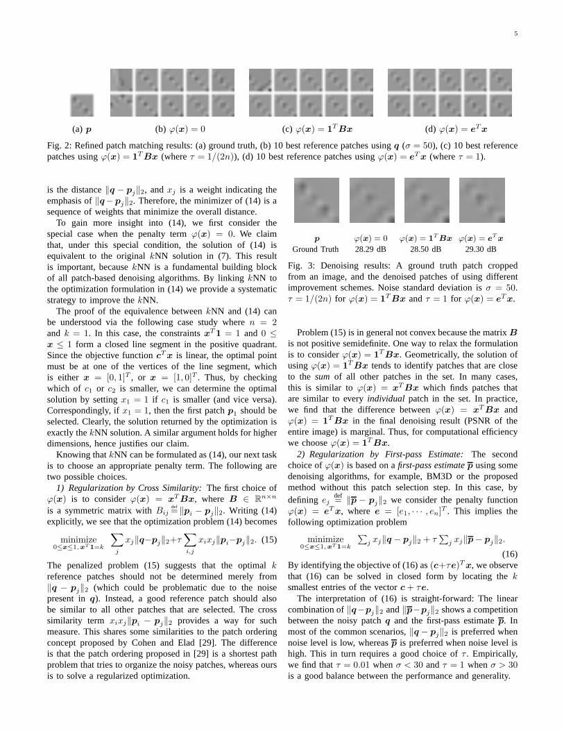
Fig. 2: Refined patch matching results: (a) ground truth, (b)10 best reference patches usingq (σ = 50), (c) 10 best referencepatches usingϕ(x) = 1

TBx (whereτ = 1/(2n)), (d) 10 best reference patches usingϕ(x) = eTx (whereτ = 1).

is the distance‖q − pj‖2, andxj is a weight indicating theemphasis of‖q−pj‖2. Therefore, the minimizer of (14) is asequence of weights that minimize the overall distance.

To gain more insight into (14), we first consider thespecial case when the penalty termϕ(x) = 0. We claimthat, under this special condition, the solution of (14) isequivalent to the originalkNN solution in (7). This resultis important, becausekNN is a fundamental building blockof all patch-based denoising algorithms. By linkingkNN tothe optimization formulation in (14) we provide a systematicstrategy to improve thekNN.

The proof of the equivalence betweenkNN and (14) canbe understood via the following case study wheren = 2and k = 1. In this case, the constraintsxT

1 = 1 and 0 ≤x ≤ 1 form a closed line segment in the positive quadrant.Since the objective functioncTx is linear, the optimal pointmust be at one of the vertices of the line segment, whichis either x = [0, 1]T , or x = [1, 0]T . Thus, by checkingwhich of c1 or c2 is smaller, we can determine the optimalsolution by settingx1 = 1 if c1 is smaller (and vice versa).Correspondingly, ifx1 = 1, then the first patchp1 should beselected. Clearly, the solution returned by the optimization isexactly thekNN solution. A similar argument holds for higherdimensions, hence justifies our claim.

Knowing thatkNN can be formulated as (14), our next taskis to choose an appropriate penalty term. The following aretwo possible choices.

1) Regularization by Cross Similarity:The first choice ofϕ(x) is to considerϕ(x) = xTBx, where B ∈ R

n×n

is a symmetric matrix withBijdef= ‖pi − pj‖2. Writing (14)

explicitly, we see that the optimization problem (14) becomes

minimize0≤x≤1,xT 1=k

∑

j

xj‖q−pj‖2+τ∑

i,j

xixj‖pi−pj‖2. (15)

The penalized problem (15) suggests that the optimalkreference patches should not be determined merely from‖q − pj‖2 (which could be problematic due to the noisepresent inq). Instead, a good reference patch should alsobe similar to all other patches that are selected. The crosssimilarity term xixj‖pi − pj‖2 provides a way for suchmeasure. This shares some similarities to the patch orderingconcept proposed by Cohen and Elad [29]. The differenceis that the patch ordering proposed in [29] is a shortest pathproblem that tries to organize the noisy patches, whereas oursis to solve a regularized optimization.

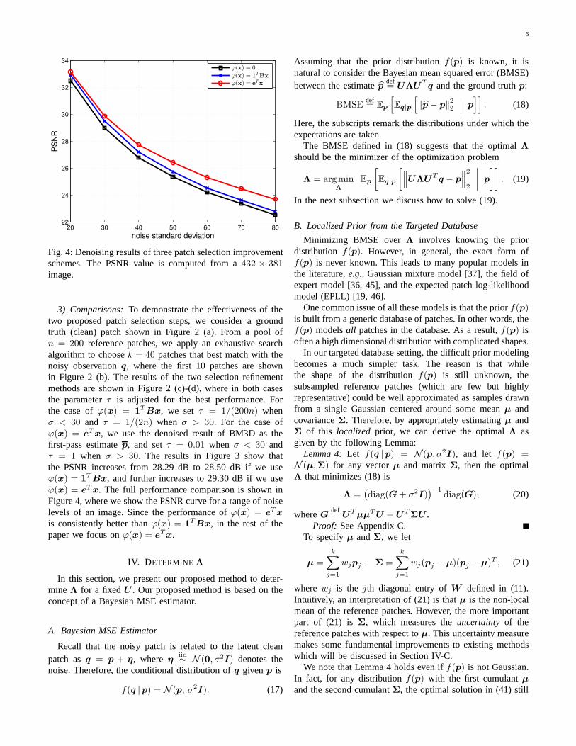
p ϕ(x) = 0 ϕ(x) = 1TBx ϕ(x) = eTx

Ground Truth 28.29 dB 28.50 dB 29.30 dB

Fig. 3: Denoising results: A ground truth patch croppedfrom an image, and the denoised patches of using differentimprovement schemes. Noise standard deviation isσ = 50.τ = 1/(2n) for ϕ(x) = 1

TBx andτ = 1 for ϕ(x) = eTx.

Problem (15) is in general not convex because the matrixB

is not positive semidefinite. One way to relax the formulationis to considerϕ(x) = 1

TBx. Geometrically, the solution ofusingϕ(x) = 1

TBx tends to identify patches that are closeto the sum of all other patches in the set. In many cases,this is similar toϕ(x) = xTBx which finds patches thatare similar to everyindividual patch in the set. In practice,we find that the difference betweenϕ(x) = xTBx andϕ(x) = 1

TBx in the final denoising result (PSNR of theentire image) is marginal. Thus, for computational efficiencywe chooseϕ(x) = 1

TBx.2) Regularization by First-pass Estimate:The second

choice ofϕ(x) is based on afirst-pass estimatep using somedenoising algorithms, for example, BM3D or the proposedmethod without this patch selection step. In this case, bydefining ej

def= ‖p − pj‖2 we consider the penalty function

ϕ(x) = eTx, where e = [e1, · · · , en]T . This implies thefollowing optimization problem

minimize0≤x≤1,xT1=k

∑j xj‖q − pj‖2 + τ

∑j xj‖p− pj‖2.

(16)By identifying the objective of (16) as(c+τe)Tx, we observethat (16) can be solved in closed form by locating theksmallest entries of the vectorc+ τe.

The interpretation of (16) is straight-forward: The linearcombination of‖q−pj‖2 and‖p−pj‖2 shows a competitionbetween the noisy patchq and the first-pass estimatep. Inmost of the common scenarios,‖q − pj‖2 is preferred whennoise level is low, whereasp is preferred when noise level ishigh. This in turn requires a good choice ofτ . Empirically,we find thatτ = 0.01 whenσ < 30 andτ = 1 whenσ > 30is a good balance between the performance and generality.

6

20 30 40 50 60 70 8022

24

26

28

30

32

34

noise standard deviation

PS

NR

ϕ(x) = 0ϕ(x) = 1

TBx

ϕ(x) = eTx

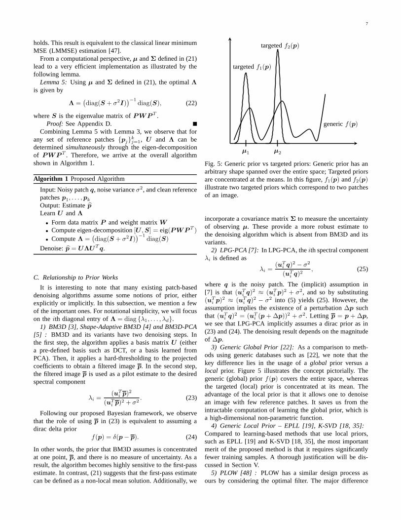
Fig. 4: Denoising results of three patch selection improvementschemes. The PSNR value is computed from a432 × 381image.

3) Comparisons:To demonstrate the effectiveness of thetwo proposed patch selection steps, we consider a groundtruth (clean) patch shown in Figure 2 (a). From a pool ofn = 200 reference patches, we apply an exhaustive searchalgorithm to choosek = 40 patches that best match with thenoisy observationq, where the first 10 patches are shownin Figure 2 (b). The results of the two selection refinementmethods are shown in Figure 2 (c)-(d), where in both casesthe parameterτ is adjusted for the best performance. Forthe case ofϕ(x) = 1

TBx, we set τ = 1/(200n) whenσ < 30 and τ = 1/(2n) when σ > 30. For the case ofϕ(x) = eTx, we use the denoised result of BM3D as thefirst-pass estimatep, and setτ = 0.01 when σ < 30 andτ = 1 when σ > 30. The results in Figure 3 show thatthe PSNR increases from 28.29 dB to 28.50 dB if we useϕ(x) = 1

TBx, and further increases to 29.30 dB if we useϕ(x) = eTx. The full performance comparison is shown inFigure 4, where we show the PSNR curve for a range of noiselevels of an image. Since the performance ofϕ(x) = eTx

is consistently better thanϕ(x) = 1TBx, in the rest of the

paper we focus onϕ(x) = eTx.

IV. D ETERMINE Λ

In this section, we present our proposed method to deter-mineΛ for a fixedU . Our proposed method is based on theconcept of a Bayesian MSE estimator.

A. Bayesian MSE Estimator

Recall that the noisy patch is related to the latent cleanpatch asq = p + η, whereη

iid∼ N (0, σ2I) denotes thenoise. Therefore, the conditional distribution ofq givenp is

f(q |p) = N (p, σ2I). (17)

Assuming that the prior distributionf(p) is known, it isnatural to consider the Bayesian mean squared error (BMSE)between the estimatep

def= UΛUTq and the ground truthp:

BMSEdef= Ep

[Eq|p

[‖p− p‖22

∣∣∣ p]]

. (18)

Here, the subscripts remark the distributions under which theexpectations are taken.

The BMSE defined in (18) suggests that the optimalΛ

should be the minimizer of the optimization problem

Λ = argminΛ

Ep

[Eq|p

[∥∥∥UΛUTq − p

∥∥∥2

2

∣∣∣∣ p

]]. (19)

In the next subsection we discuss how to solve (19).

B. Localized Prior from the Targeted Database

Minimizing BMSE over Λ involves knowing the priordistribution f(p). However, in general, the exact form off(p) is never known. This leads to many popular models inthe literature,e.g., Gaussian mixture model [37], the field ofexpert model [36, 45], and the expected patch log-likelihoodmodel (EPLL) [19, 46].

One common issue of all these models is that the priorf(p)is built from a generic database of patches. In other words, thef(p) modelsall patches in the database. As a result,f(p) isoften a high dimensional distribution with complicated shapes.

In our targeted database setting, the difficult prior modelingbecomes a much simpler task. The reason is that whilethe shape of the distributionf(p) is still unknown, thesubsampled reference patches (which are few but highlyrepresentative) could be well approximated as samples drawnfrom a single Gaussian centered around some meanµ andcovarianceΣ. Therefore, by appropriately estimatingµ andΣ of this localized prior, we can derive the optimalΛ asgiven by the following Lemma:

Lemma 4:Let f(q |p) = N (p, σ2I), and let f(p) =N (µ,Σ) for any vectorµ and matrixΣ, then the optimalΛ that minimizes (18) is

Λ =(diag(G+ σ2I)

)−1diag(G), (20)

whereGdef= UTµµTU +UT

ΣU .Proof: See Appendix C.

To specifyµ andΣ, we let

µ =

k∑

j=1

wjpj , Σ =

k∑

j=1

wj(pj − µ)(pj − µ)T , (21)

wherewj is the jth diagonal entry ofW defined in (11).Intuitively, an interpretation of (21) is thatµ is the non-localmean of the reference patches. However, the more importantpart of (21) isΣ, which measures theuncertainty of thereference patches with respect toµ. This uncertainty measuremakes some fundamental improvements to existing methodswhich will be discussed in Section IV-C.

We note that Lemma 4 holds even iff(p) is not Gaussian.In fact, for any distributionf(p) with the first cumulantµand the second cumulantΣ, the optimal solution in (41) still

7

holds. This result is equivalent to the classical linear minimumMSE (LMMSE) estimation [47].

From a computational perspective,µ andΣ defined in (21)lead to a very efficient implementation as illustrated by thefollowing lemma.

Lemma 5:Using µ andΣ defined in (21), the optimalΛis given by

Λ =(diag(S + σ2I)

)−1diag(S), (22)

whereS is the eigenvalue matrix ofPWP T .Proof: See Appendix D.

Combining Lemma 5 with Lemma 3, we observe that forany set of reference patches{pj}kj=1, U and Λ can bedeterminedsimultaneouslythrough the eigen-decompositionof PWP T . Therefore, we arrive at the overall algorithmshown in Algorithm 1.

Algorithm 1 Proposed Algorithm

Input: Noisy patchq, noise varianceσ2, and clean referencepatchesp1, . . . ,pk

Output: EstimatepLearnU andΛ

• Form data matrixP and weight matrixW• Compute eigen-decomposition[U ,S] = eig(PWP T )

• ComputeΛ =(diag(S + σ2I)

)−1diag(S)

Denoise:p = UΛUTq.

C. Relationship to Prior Works

It is interesting to note that many existing patch-baseddenoising algorithms assume some notions of prior, eitherexplicitly or implicitly. In this subsection, we mention a fewof the important ones. For notational simplicity, we will focuson theith diagonal entry ofΛ = diag {λ1, . . . , λd}.

1) BM3D [3], Shape-Adaptive BM3D [4] and BM3D-PCA[5] : BM3D and its variants have two denoising steps. Inthe first step, the algorithm applies a basis matrixU (eithera pre-defined basis such as DCT, or a basis learned fromPCA). Then, it applies a hard-thresholding to the projectedcoefficients to obtain a filtered imagep. In the second step,the filtered imagep is used as a pilot estimate to the desiredspectral component

λi =(uT

i p)2

(uTi p)

2 + σ2. (23)

Following our proposed Bayesian framework, we observethat the role of usingp in (23) is equivalent to assuming adirac delta prior

f(p) = δ(p− p). (24)

In other words, the prior that BM3D assumes is concentratedat one point,p, and there is no measure of uncertainty. As aresult, the algorithm becomes highly sensitive to the first-passestimate. In contrast, (21) suggests that the first-pass estimatecan be defined as a non-local mean solution. Additionally, we

µ1 µ2

targetedf1(p)

targetedf2(p)

genericf(p)

Fig. 5: Generic prior vs targeted priors: Generic prior has anarbitrary shape spanned over the entire space; Targeted priorsare concentrated at the means. In this figure,f1(p) andf2(p)illustrate two targeted priors which correspond to two patchesof an image.

incorporate a covariance matrixΣ to measure the uncertaintyof observingµ. These provide a more robust estimate tothe denoising algorithm which is absent from BM3D and itsvariants.

2) LPG-PCA [7]: In LPG-PCA, theith spectral componentλi is defined as

λi =(uT

i q)2 − σ2

(uTi q)

2, (25)

where q is the noisy patch. The (implicit) assumption in[7] is that (uT

i q)2 ≈ (uT

i p)2 + σ2, and so by substituting

(uTi p)

2 ≈ (uTi q)

2 − σ2 into (5) yields (25). However, theassumption implies the existence of a perturbation∆p suchthat (uT

i q)2 = (uT

i (p + ∆p))2 + σ2. Letting p = p + ∆p,we see that LPG-PCA implicitly assumes a dirac prior as in(23) and (24). The denoising result depends on the magnitudeof ∆p.

3) Generic Global Prior [22]: As a comparison to meth-ods using generic databases such as [22], we note that thekey difference lies in the usage of aglobal prior versus alocal prior. Figure 5 illustrates the concept pictorially. Thegeneric (global) priorf(p) covers the entire space, whereasthe targeted (local) prior is concentrated at its mean. Theadvantage of the local prior is that it allows one to denoisean image with few reference patches. It saves us from theintractable computation of learning the global prior, which isa high-dimensional non-parametric function.

4) Generic Local Prior – EPLL [19], K-SVD [18, 35]:Compared to learning-based methods that use local priors,such as EPLL [19] and K-SVD [18, 35], the most importantmerit of the proposed method is that it requires significantlyfewer training samples. A thorough justification will be dis-cussed in Section V.

5) PLOW [48] : PLOW has a similar design process asours by considering the optimal filter. The major difference

8

is that in PLOW, the denoising filter is derived from the fullcovariance matrices of the data and noise. As we will see inthe next subsection, the linear denoising filter of our workis a truncated SVD matrix computed from a set of similarpatches. The merit of the truncation is that it often reducesMSE in the bias-variance trade off [42].

D. ImprovingΛ

The Bayesian framework proposed above can be general-ized to further improve the denoising performance. Referringto (19), we observe that the BMSE optimization can bereformulated to incorporate a penalty term inΛ. Here, weconsider the followingℓα penalized BMSE:

BMSEαdef= Ep

[Eq|p

[∥∥∥UΛUTq − p

∥∥∥2

2

∣∣∣∣p]]

+ γ‖Λ1‖α,(26)

whereγ > 0 is the penalty parameter, andα ∈ {0, 1} controlswhich norm to be used. The solution to the minimization of(26) is given by the following lemma.

Lemma 6:Let si be theith diagonal entry inS, whereSis the eigenvalue matrix ofPWP T , then the optimalΛ thatminimizes BMSEα is diag {λ1, · · · , λd}, where

λi = max

(si − γ/2

si + σ2, 0

), for α = 1, (27)

λi =si

si + σ21

(s2i

si + σ2> γ

), for α = 0. (28)

Proof: See Appendix E.The motivation of introducing anℓα-norm penalty in (26)

is related the group sparsity used in definingU . Recallfrom Section III that sinceU is the optimal solution to agroup sparsity optimization, only few of the entries in theideal projectionUTp should be non-zero. Consequently, it isdesired to requireΛ to be sparse so thatUΛUT q has similarspectral components as that ofp.

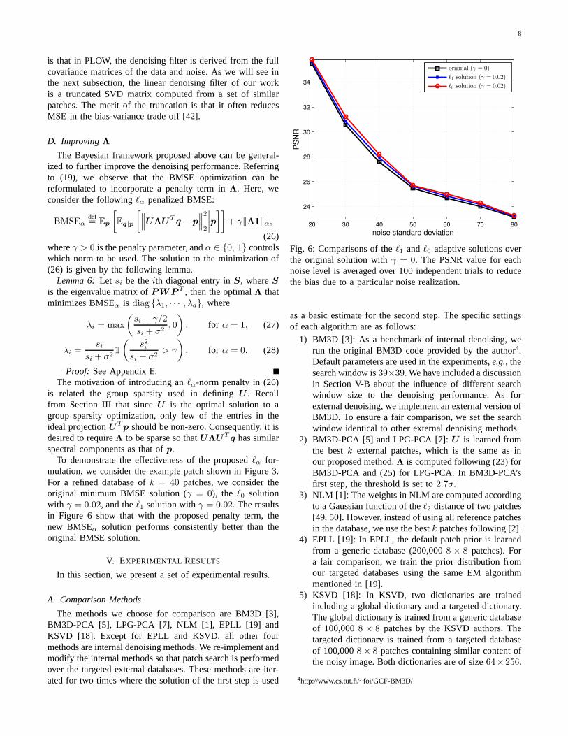
To demonstrate the effectiveness of the proposedℓα for-mulation, we consider the example patch shown in Figure 3.For a refined database ofk = 40 patches, we consider theoriginal minimum BMSE solution (γ = 0), the ℓ0 solutionwith γ = 0.02, and theℓ1 solution withγ = 0.02. The resultsin Figure 6 show that with the proposed penalty term, thenew BMSEα solution performs consistently better than theoriginal BMSE solution.

V. EXPERIMENTAL RESULTS

In this section, we present a set of experimental results.

A. Comparison Methods

The methods we choose for comparison are BM3D [3],BM3D-PCA [5], LPG-PCA [7], NLM [1], EPLL [19] andKSVD [18]. Except for EPLL and KSVD, all other fourmethods are internal denoising methods. We re-implement andmodify the internal methods so that patch search is performedover the targeted external databases. These methods are iter-ated for two times where the solution of the first step is used

20 30 40 50 60 70 80

24

26

28

30

32

34

noise standard deviation

PS

NR

original (γ = 0)

ℓ1 solution (γ = 0.02)

ℓ0 solution (γ = 0.02)

Fig. 6: Comparisons of theℓ1 andℓ0 adaptive solutions overthe original solution withγ = 0. The PSNR value for eachnoise level is averaged over 100 independent trials to reducethe bias due to a particular noise realization.

as a basic estimate for the second step. The specific settingsof each algorithm are as follows:

1) BM3D [3]: As a benchmark of internal denoising, werun the original BM3D code provided by the author4.Default parameters are used in the experiments,e.g., thesearch window is39×39. We have included a discussionin Section V-B about the influence of different searchwindow size to the denoising performance. As forexternal denoising, we implement an external version ofBM3D. To ensure a fair comparison, we set the searchwindow identical to other external denoising methods.

2) BM3D-PCA [5] and LPG-PCA [7]:U is learned fromthe bestk external patches, which is the same as inour proposed method.Λ is computed following (23) forBM3D-PCA and (25) for LPG-PCA. In BM3D-PCA’sfirst step, the threshold is set to2.7σ.

3) NLM [1]: The weights in NLM are computed accordingto a Gaussian function of theℓ2 distance of two patches[49, 50]. However, instead of using all reference patchesin the database, we use the bestk patches following [2].

4) EPLL [19]: In EPLL, the default patch prior is learnedfrom a generic database (200,0008 × 8 patches). Fora fair comparison, we train the prior distribution fromour targeted databases using the same EM algorithmmentioned in [19].

5) KSVD [18]: In KSVD, two dictionaries are trainedincluding a global dictionary and a targeted dictionary.The global dictionary is trained from a generic databaseof 100,0008 × 8 patches by the KSVD authors. Thetargeted dictionary is trained from a targeted databaseof 100,0008 × 8 patches containing similar content ofthe noisy image. Both dictionaries are of size64× 256.

4http://www.cs.tut.fi/~foi/GCF-BM3D/

9

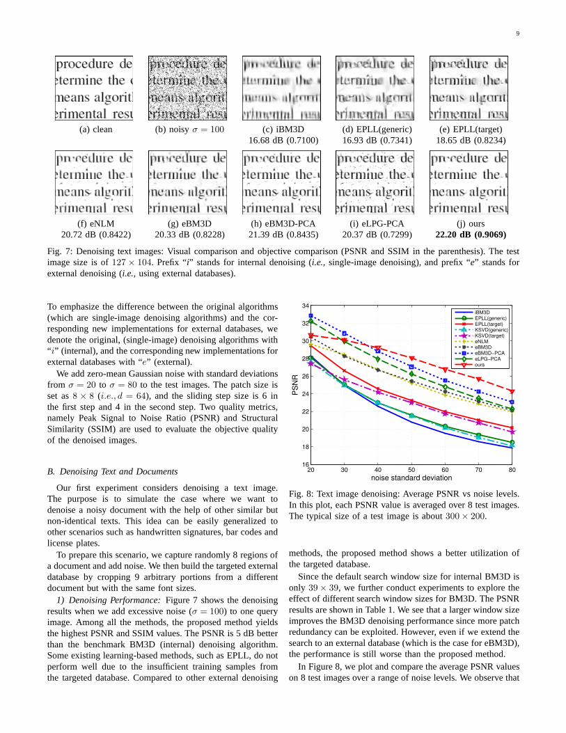
(a) clean (b) noisyσ = 100 (c) iBM3D (d) EPLL(generic) (e) EPLL(target)16.68 dB (0.7100) 16.93 dB (0.7341) 18.65 dB (0.8234)

(f) eNLM (g) eBM3D (h) eBM3D-PCA (i) eLPG-PCA (j) ours20.72 dB (0.8422) 20.33 dB (0.8228) 21.39 dB (0.8435) 20.37 dB (0.7299) 22.20 dB (0.9069)

Fig. 7: Denoising text images: Visual comparison and objective comparison (PSNR and SSIM in the parenthesis). The testimage size is of127 × 104. Prefix “i” stands for internal denoising (i.e., single-image denoising), and prefix “e” stands forexternal denoising (i.e., using external databases).

To emphasize the difference between the original algorithms(which are single-image denoising algorithms) and the cor-responding new implementations for external databases, wedenote the original, (single-image) denoising algorithmswith“ i” (internal), and the corresponding new implementations forexternal databases with “e” (external).

We add zero-mean Gaussian noise with standard deviationsfrom σ = 20 to σ = 80 to the test images. The patch size isset as8 × 8 (i.e., d = 64), and the sliding step size is 6 inthe first step and 4 in the second step. Two quality metrics,namely Peak Signal to Noise Ratio (PSNR) and StructuralSimilarity (SSIM) are used to evaluate the objective qualityof the denoised images.

B. Denoising Text and Documents

Our first experiment considers denoising a text image.The purpose is to simulate the case where we want todenoise a noisy document with the help of other similar butnon-identical texts. This idea can be easily generalized toother scenarios such as handwritten signatures, bar codes andlicense plates.

To prepare this scenario, we capture randomly 8 regions ofa document and add noise. We then build the targeted externaldatabase by cropping 9 arbitrary portions from a differentdocument but with the same font sizes.

1) Denoising Performance:Figure 7 shows the denoisingresults when we add excessive noise (σ = 100) to one queryimage. Among all the methods, the proposed method yieldsthe highest PSNR and SSIM values. The PSNR is 5 dB betterthan the benchmark BM3D (internal) denoising algorithm.Some existing learning-based methods, such as EPLL, do notperform well due to the insufficient training samples fromthe targeted database. Compared to other external denoising

20 30 40 50 60 70 8016

18

20

22

24

26

28

30

32

34

noise standard deviation

PS

NR

iBM3DEPLL(generic)EPLL(target)KSVD(generic)KSVD(target)eNLMeBM3DeBM3D−PCAeLPG−PCAours

Fig. 8: Text image denoising: Average PSNR vs noise levels.In this plot, each PSNR value is averaged over 8 test images.The typical size of a test image is about300× 200.

methods, the proposed method shows a better utilization ofthe targeted database.

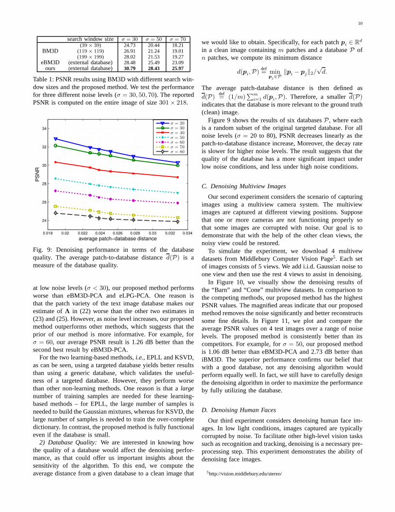
Since the default search window size for internal BM3D isonly 39× 39, we further conduct experiments to explore theeffect of different search window sizes for BM3D. The PSNRresults are shown in Table 1. We see that a larger window sizeimproves the BM3D denoising performance since more patchredundancy can be exploited. However, even if we extend thesearch to an external database (which is the case for eBM3D),the performance is still worse than the proposed method.

In Figure 8, we plot and compare the average PSNR valueson 8 test images over a range of noise levels. We observe that

10

search window size σ = 30 σ = 50 σ = 70

BM3D(39× 39) 24.73 20.44 18.21

(119 × 119) 26.91 21.24 19.01(199 × 199) 28.02 21.53 19.27

eBM3D (external database) 28.48 25.49 23.09ours (external database) 30.79 28.43 25.97

Table 1: PSNR results using BM3D with different search win-dow sizes and the proposed method. We test the performancefor three different noise levels (σ = 30, 50, 70). The reportedPSNR is computed on the entire image of size301× 218.

0.018 0.02 0.022 0.024 0.026 0.028 0.03 0.032 0.034

24

26

28

30

32

34

average patch−database distance

PS

NR

σ = 20σ = 30σ = 40σ = 50σ = 60σ = 70σ = 80

Fig. 9: Denoising performance in terms of the databasequality. The average patch-to-database distanced(P) is ameasure of the database quality.

at low noise levels (σ < 30), our proposed method performsworse than eBM3D-PCA and eLPG-PCA. One reason isthat the patch variety of the text image database makes ourestimate ofΛ in (22) worse than the other two estimates in(23) and (25). However, as noise level increases, our proposedmethod outperforms other methods, which suggests that theprior of our method is more informative. For example, forσ = 60, our average PSNR result is 1.26 dB better than thesecond best result by eBM3D-PCA.

For the two learning-based methods,i.e.,EPLL and KSVD,as can be seen, using a targeted database yields better resultsthan using a generic database, which validates the useful-ness of a targeted database. However, they perform worsethan other non-learning methods. One reason is that alargenumber of training samples are needed for these learning-based methods – for EPLL, the large number of samples isneeded to build the Gaussian mixtures, whereas for KSVD, thelarge number of samples is needed to train the over-completedictionary. In contrast, the proposed method is fully functionaleven if the database is small.

2) Database Quality:We are interested in knowing howthe quality of a database would affect the denoising perfor-mance, as that could offer us important insights about thesensitivity of the algorithm. To this end, we compute theaverage distance from a given database to a clean image that

we would like to obtain. Specifically, for each patchpi ∈ Rd

in a clean image containingm patches and a databaseP ofn patches, we compute its minimum distance

d(pi,P)def= min

pj∈P‖pi − pj‖2/

√d.

The average patch-database distance is then defined asd(P)

def= (1/m)

∑mi=1 d(pi,P). Therefore, a smallerd(P)

indicates that the database is more relevant to the ground truth(clean) image.

Figure 9 shows the results of six databasesP , where eachis a random subset of the original targeted database. For allnoise levels (σ = 20 to 80), PSNR decreases linearly as thepatch-to-database distance increase, Moreover, the decayrateis slower for higher noise levels. The result suggests that thequality of the database has a more significant impact underlow noise conditions, and less under high noise conditions.

C. Denoising Multiview Images

Our second experiment considers the scenario of capturingimages using a multiview camera system. The multiviewimages are captured at different viewing positions. Supposethat one or more cameras are not functioning properly sothat some images are corrupted with noise. Our goal is todemonstrate that with the help of the other clean views, thenoisy view could be restored.

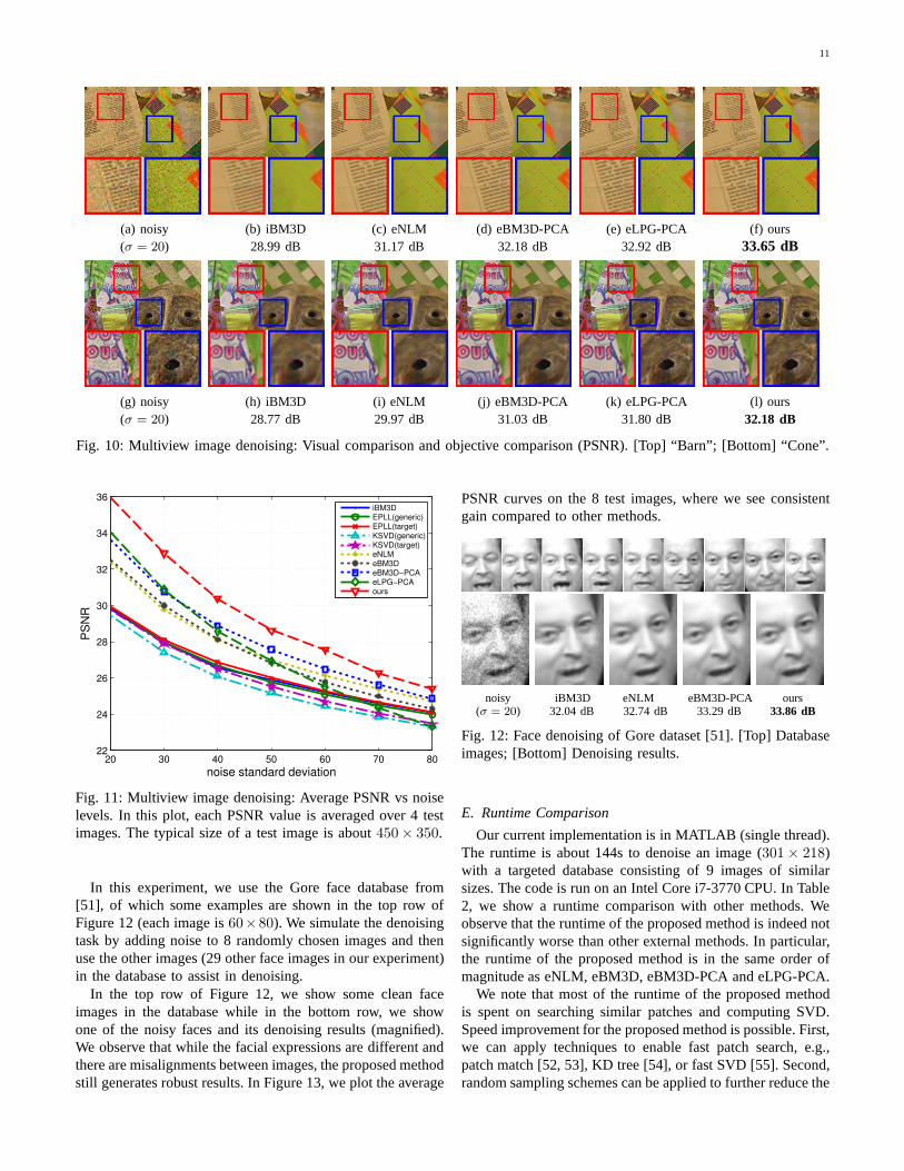
To simulate the experiment, we download 4 multivewdatasets from Middlebury Computer Vision Page5. Each setof images consists of 5 views. We add i.i.d. Gaussian noise toone view and then use the rest 4 views to assist in denoising.

In Figure 10, we visually show the denoising results ofthe “Barn” and “Cone” multiview datasets. In comparison tothe competing methods, our proposed method has the highestPSNR values. The magnified areas indicate that our proposedmethod removes the noise significantly and better reconstructssome fine details. In Figure 11, we plot and compare theaverage PSNR values on 4 test images over a range of noiselevels. The proposed method is consistently better than itscompetitors. For example, forσ = 50, our proposed methodis 1.06 dB better than eBM3D-PCA and 2.73 dB better thaniBM3D. The superior performance confirms our belief thatwith a good database, not any denoising algorithm wouldperform equally well. In fact, we still have to carefully designthe denoising algorithm in order to maximize the performanceby fully utilizing the database.

D. Denoising Human Faces

Our third experiment considers denoising human face im-ages. In low light conditions, images captured are typicallycorrupted by noise. To facilitate other high-level vision taskssuch as recognition and tracking, denoising is a necessary pre-processing step. This experiment demonstrates the abilityofdenoising face images.

5http://vision.middlebury.edu/stereo/

11

(a) noisy (b) iBM3D (c) eNLM (d) eBM3D-PCA (e) eLPG-PCA (f) ours(σ = 20) 28.99 dB 31.17 dB 32.18 dB 32.92 dB 33.65 dB

(g) noisy (h) iBM3D (i) eNLM (j) eBM3D-PCA (k) eLPG-PCA (l) ours(σ = 20) 28.77 dB 29.97 dB 31.03 dB 31.80 dB 32.18 dB

Fig. 10: Multiview image denoising: Visual comparison and objective comparison (PSNR). [Top] “Barn”; [Bottom] “Cone”.

20 30 40 50 60 70 8022

24

26

28

30

32

34

36

noise standard deviation

PS

NR

iBM3DEPLL(generic)EPLL(target)KSVD(generic)KSVD(target)eNLMeBM3DeBM3D−PCAeLPG−PCAours

Fig. 11: Multiview image denoising: Average PSNR vs noiselevels. In this plot, each PSNR value is averaged over 4 testimages. The typical size of a test image is about450× 350.

In this experiment, we use the Gore face database from[51], of which some examples are shown in the top row ofFigure 12 (each image is60×80). We simulate the denoisingtask by adding noise to 8 randomly chosen images and thenuse the other images (29 other face images in our experiment)in the database to assist in denoising.

In the top row of Figure 12, we show some clean faceimages in the database while in the bottom row, we showone of the noisy faces and its denoising results (magnified).We observe that while the facial expressions are different andthere are misalignments between images, the proposed methodstill generates robust results. In Figure 13, we plot the average

PSNR curves on the 8 test images, where we see consistentgain compared to other methods.

noisy(σ = 20)

iBM3D32.04 dB

eNLM32.74 dB

eBM3D-PCA33.29 dB

ours33.86 dB

Fig. 12: Face denoising of Gore dataset [51]. [Top] Databaseimages; [Bottom] Denoising results.

E. Runtime Comparison

Our current implementation is in MATLAB (single thread).The runtime is about 144s to denoise an image (301× 218)with a targeted database consisting of 9 images of similarsizes. The code is run on an Intel Core i7-3770 CPU. In Table2, we show a runtime comparison with other methods. Weobserve that the runtime of the proposed method is indeed notsignificantly worse than other external methods. In particular,the runtime of the proposed method is in the same order ofmagnitude as eNLM, eBM3D, eBM3D-PCA and eLPG-PCA.

We note that most of the runtime of the proposed methodis spent on searching similar patches and computing SVD.Speed improvement for the proposed method is possible. First,we can apply techniques to enable fast patch search, e.g.,patch match [52, 53], KD tree [54], or fast SVD [55]. Second,random sampling schemes can be applied to further reduce the

12

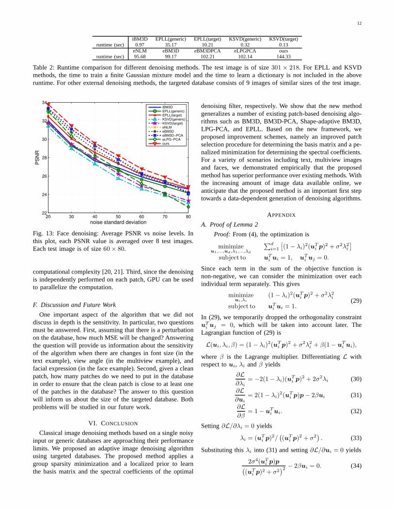
iBM3D EPLL(generic) EPLL(target) KSVD(generic) KSVD(target)runtime (sec) 0.97 35.17 10.21 0.32 0.13

eNLM eBM3D eBM3DPCA eLPGPCA oursruntime (sec) 95.68 99.17 102.21 102.14 144.33

Table 2: Runtime comparison for different denoising methods. The test image is of size301 × 218. For EPLL and KSVDmethods, the time to train a finite Gaussian mixture model andthe time to learn a dictionary is not included in the aboveruntime. For other external denoising methods, the targeted database consists of 9 images of similar sizes of the test image.

20 30 40 50 60 70 8022

24

26

28

30

32

34

noise standard deviation

PS

NR

iBM3DEPLL(generic)EPLL(target)KSVD(generic)KSVD(target)eNLMeBM3DeBM3D−PCAeLPG−PCAours

Fig. 13: Face denoising: Average PSNR vs noise levels. Inthis plot, each PSNR value is averaged over 8 test images.Each test image is of size60× 80.

computational complexity [20, 21]. Third, since the denoisingis independently performed on each patch, GPU can be usedto parallelize the computation.

F. Discussion and Future Work

One important aspect of the algorithm that we did notdiscuss in depth is the sensitivity. In particular, two questionsmust be answered. First, assuming that there is a perturbationon the database, how much MSE will be changed? Answeringthe question will provide us information about the sensitivityof the algorithm when there are changes in font size (in thetext example), view angle (in the multiview example), andfacial expression (in the face example). Second, given a cleanpatch, how many patches do we need to put in the databasein order to ensure that the clean patch is close to at least oneof the patches in the database? The answer to this questionwill inform us about the size of the targeted database. Bothproblems will be studied in our future work.

VI. CONCLUSION

Classical image denoising methods based on a single noisyinput or generic databases are approaching their performancelimits. We proposed an adaptive image denoising algorithmusing targeted databases. The proposed method applies agroup sparsity minimization and a localized prior to learnthe basis matrix and the spectral coefficients of the optimal

denoising filter, respectively. We show that the new methodgeneralizes a number of existing patch-based denoising algo-rithms such as BM3D, BM3D-PCA, Shape-adaptive BM3D,LPG-PCA, and EPLL. Based on the new framework, weproposed improvement schemes, namely an improved patchselection procedure for determining the basis matrix and a pe-nalized minimization for determining the spectral coefficients.For a variety of scenarios including text, multiview imagesand faces, we demonstrated empirically that the proposedmethod has superior performance over existing methods. Withthe increasing amount of image data available online, weanticipate that the proposed method is an important first steptowards a data-dependent generation of denoising algorithms.

APPENDIX

A. Proof of Lemma 2

Proof: From (4), the optimization is

minimizeu1,...,ud,λ1,...,λd

∑di=1

[(1− λi)

2(uTi p)

2 + σ2λ2i

]

subject to uTi ui = 1, uT

i uj = 0.

Since each term in the sum of the objective function isnon-negative, we can consider the minimization over eachindividual term separately. This gives

minimizeui,λi

(1− λi)2(uT

i p)2 + σ2λ2

i

subject to uTi ui = 1.

(29)

In (29), we temporarily dropped the orthogonality constraintuTi uj = 0, which will be taken into account later. The

Lagrangian function of (29) is

L(ui, λi, β) = (1− λi)2(uT

i p)2 + σ2λ2

i + β(1− uTi ui),

whereβ is the Lagrange multiplier. DifferentiatingL withrespect toui, λi andβ yields

∂L∂λi

= −2(1− λi)(uTi p)

2 + 2σ2λi (30)

∂L∂ui

= 2(1− λi)2(uT

i p)p− 2βui (31)

∂L∂β

= 1− uTi ui. (32)

Setting∂L/∂λi = 0 yields

λi = (uTi p)

2/((uT

i p)2 + σ2

). (33)

Substituting thisλi into (31) and setting∂L/∂ui = 0 yields

2σ4(uTi p)p(

(uTi p)

2 + σ2)2 − 2βui = 0. (34)

13

Therefore, the optimal pair (ui, β) of (29) must be the solutionof (34). The correspondingλi can be calculated via (33).

Referring to (34), we observe two possible scenarios. First,if ui is any unit vector orthogonal topi, andβ = 0, then(34) can be satisfied. This is a trivial solution, becauseui⊥p

impliesuTi p = 0, and henceλi = 0. The second case is that

ui = p/‖p‖2, and β =σ4‖p‖2

(‖p‖2 + σ2)2. (35)

Substituting (35) shows that (34) is satisfied. This is thenon-trivial solution. The correspondingλi in this case is‖p‖2/(‖p‖2 + σ2).

Finally, taking into account of the orthogonality constraintuTi uj = 0 if i 6= j, we can chooseu1 = p/‖p‖2, and

u2⊥u1, u3⊥{u1,u2}, . . ., ud⊥{u1,u2, . . .ud−1}. There-fore, the denoising result is

p = U

(diag

{ ‖p‖2‖p‖2 + σ2

, 0, . . . , 0

})UTq,

where U is any orthonormal matrix with the first columnu1 = p/‖p‖2.

B. Proof of Lemma 3

Proof: Let ui be theith column ofU . Then, (9) becomes

minimizeu1,...,ud

∑di=1 ‖uT

i P ‖2subject to uT

i ui = 1, uTi uj = 0.

(36)

Since each term in the sum of (36) is non-negative, we canconsider each individual term

minimizeui

‖uTi P ‖2

subject to uTi ui = 1,

which is equivalent to

minimizeui

‖uTi P ‖22

subject to uTi ui = 1.

(37)

The constrained problem (37) can be solved by consideringthe Lagrange function,

L(ui, β) = ‖uTi P ‖22 + β(1− uT

i ui). (38)

Taking derivatives∂L∂ui

= 0 and ∂L∂β = 0 yield

PP Tui = βui, and uTi ui = 1.

Therefore,ui is the eigenvector ofPP T , andβ is the corre-sponding eigenvalue. Since the eigenvectors are orthonormalto each other, the solution automatically satisfies the orthog-onality constraint thatuT

i uj = 0 if i 6= j.

C. Proof of Lemma 4

Proof: First, by pluggingq = p+ η into BMSE we get

BMSE = Ep

[Eq|p

[∥∥∥UΛUT (p+ η)− p∥∥∥2

2

∣∣∣∣p]]

= Ep

[pTU (I −Λ)

2UTp

]+ σ2Tr

(Λ

2).

Recall the fact that for any random variablex ∼ N (µx,Σx)and any matrixA, it holds thatE

[xTAx

]= E[x]TAE[x]+

Tr (AΣx). Therefore, the above BMSE can be simplified as

µTU(I −Λ)2UTµ+Tr(U(I −Λ)2UT

Σ

)+ σ2Tr

(Λ

2)

=Tr((I −Λ)2UTµµTU + (I −Λ)2UT

ΣU)+ σ2Tr

(Λ

2)

=Tr((I −Λ)2G

)+ σ2Tr(Λ2)

=

d∑

i=1

[(1 − λi)

2gi + σ2λ2i

], (39)

whereGdef= UTµµTU +UT

ΣU andgi is the ith diagonalentry inG.

Setting∂BMSE/∂λi = 0 yields

2(1− λi)gi + 2σ2λi = 0. (40)

Therefore, the optimalλi is gi/(gi + σ2) and the optimalΛis

Λ = diag

{g1

g1 + σ2, · · · , gd

gd + σ2

}, (41)

which, by definition, is(diag(G+ σ2I)

)−1diag(G).

D. Proof of Lemma 5

Proof: First, we writeΣ in (21) in the matrix form

Σ =(P − µ1T

)W

(P − µ1T

)T

= PWP T − µ1TWP T − PW1µT + µ1TW1µT .

It is not difficult to see that1TWP T = µT ,PW1 = µ and1TW1 = 1. Therefore,

Σ = PWP T − µµT − µµT + µµT = PWP T − µµT ,

which gives

µµT +Σ = PWP T . (42)

Note thatG = UTµµTU + UTΣU = UT (µµT + Σ)U .

Substituting (42) intoG and using equation (10), we have

G = UTPWP TU = UTUSUTU = S.

Therefore, by Lemma 4,

Λ =(diag(S + σ2I)

)−1diag(S). (43)

14

E. Proof of Lemma 6

By Lemma 5, it holds that

Ep

[Eq|p

[∥∥∥UΛUTq − p∥∥∥2

2

∣∣∣∣p]]

=

d∑

i=1

[(1− λi)

2si + σ2λ2i

]

=

d∑

i=1

[(si + σ2)

(λi −

sisi + σ2

)2

+siσ

2

si + σ2

].

Therefore, the minimization of (26) becomes

minimizeλi

d∑

i=1

[(si + σ2)

(λi −

sisi + σ2

)2]+ γ‖Λ1‖α,

(44)where γ‖Λ1‖α = γ

∑di=1 |λi| or γ

∑di=1 1(λi 6= 0) for

α = 1 or 0. We note that whenα = 1 or 0, (44) is thestandard shrinkage problem [56], in which a closed formsolution exists. Following from [57], the solutions are givenby

λi = max

(si − γ/2

si + σ2, 0

), for α = 1,

and

λi =si

si + σ21

(s2i

si + σ2> γ

), for α = 0.

REFERENCES

[1] A. Buades, B. Coll, and J. Morel, “A review of image denoisingalgorithms, with a new one,”SIAM Multiscale Model and Simulation,vol. 4, no. 2, pp. 490–530, 2005.

[2] C. Kervrann and J. Boulanger, “Local adaptivity to variable smoothnessfor exemplar-based image regularization and representation,” Interna-tional Journal of Computer Vision, vol. 79, no. 1, pp. 45–69, 2008.

[3] K. Dabov, A. Foi, V. Katkovnik, and K. Egiazarian, “Imagedenoisingby sparse 3D transform-domain collaborative filtering,”IEEE Trans.Image Process., vol. 16, no. 8, pp. 2080–2095, Aug. 2007.

[4] K. Dabov, A. Foi, V. Katkovnik, and K. Egiazarian, “A nonlocaland shape-adaptive transform-domain collaborative filtering,” in Proc.Intl. Workshop on Local and Non-Local Approx. in Image Process.(LNLA’08), pp. 1–8, Aug. 2008.

[5] K. Dabov, A. Foi, V. Katkovnik, and K. Egiazarian, “BM3D imagedenoising with shape-adaptive principal component analysis,” in SignalProcess. with Adaptive Sparse Structured Representations(SPARS’09),pp. 1–6, Apr. 2009.

[6] J. Mairal, F. Bach, J. Ponce, G. Sapiro, and A. Zisserman,“Non-localsparse models for image restoration,” inProc. IEEE Conf. ComputerVision and Pattern Recognition (CVPR’09), pp. 2272–2279, Sep. 2009.

[7] L. Zhang, W. Dong, D. Zhang, and G. Shi, “Two-stage image denoisingby principal component analysis with local pixel grouping,” PatternRecognition, vol. 43, pp. 1531–1549, Apr. 2010.

[8] W. Dong, L. Zhang, G. Shi, and X. Li, “Nonlocally centralized sparserepresentation for image restoration,”IEEE Trans. Image Process., vol.22, no. 4, pp. 1620 – 1630, Apr. 2013.

[9] A. Rajwade, A. Rangarajan, and A. Banerjee, “Image denoising usingthe higher order singular value decomposition,”IEEE Trans. PatternAnal. and Mach. Intell., vol. 35, no. 4, pp. 849 – 862, Apr. 2013.

[10] M. Zontak and M. Irani, “Internal statistics of a singlenatural image,” inProc. IEEE Conf. Computer Vision and Pattern Recognition (CVPR’11),pp. 977–984, Jun. 2011.

[11] I. Mosseri, M. Zontak, and M. Irani, “Combining the power ofinternal and external denoising,” inProc. Intl. Conf. ComputationalPhotography (ICCP’13), pp. 1–9, Apr. 2013.

[12] H. C. Burger, C. J. Schuler, and S. Harmeling, “Learninghow tocombine internal and external denoising methods,”Pattern Recognition,pp. 121–130, 2013.

[13] D. Glasner, S. Bagon, and M. Irani, “Super-resolution from a singleimage,” in Proc. Intl. Conf. Computer Vision (ICCV’09), pp. 349–356,Sep. 2009.

[14] P. Chatterjee and P. Milanfar, “Is denoising dead?,”IEEE Trans. ImageProcess., vol. 19, no. 4, pp. 895–911, Apr. 2010.

[15] A. Levin and B. Nadler, “Natural image denoising: Optimality andinherent bounds,” inProc. IEEE Conf. Computer Vision and PatternRecognition (CVPR’11), pp. 2833–2840, Jun. 2011.

[16] R. Yan, L. Shao, S. D. Cvetkovic, and J. Klijn, “Improvednonlocalmeans based on pre-classification and invariant block matching,” Jour-nal of Display Technology, vol. 8, no. 4, pp. 212–218, Apr. 2012.

[17] Y. Lou, P. Favaro, S. Soatto, and A. Bertozzi, “Nonlocalsimilarityimage filtering,” Lecture Notes in Computer Science, pp. 62–71.Springer Berlin Heidelberg, 2009.

[18] M. Elad and M. Aharon, “Image denoising via sparse and redundantrepresentations over learned dictionaries,”IEEE Trans. Image Process.,vol. 15, no. 12, pp. 3736–3745, Dec. 2006.

[19] D. Zoran and Y. Weiss, “From learning models of natural image patchesto whole image restoration,” inProc. IEEE Intl. Conf. Computer Vision(ICCV’11), pp. 479–486, Nov. 2011.

[20] S. H. Chan, T. Zickler, and Y. M. Lu, “Fast non-local filtering byrandom sampling: it works, especially for large images,” inProc. IEEEIntl. Conf. Acoustics, Speech and Signal Process. (ICASSP ’13), pp.1603–1607, May 2013.

[21] S. H. Chan, T. Zickler, and Y. M. Lu, “Monte Carlo non-local means:Random sampling for large-scale image filtering,”IEEE Trans. ImageProcess., vol. 23, no. 8, pp. 3711–3725, Aug. 2014.

[22] A. Levin, B. Nadler, F. Durand, and W. T. Freeman, “Patchcomplexity,finite pixel correlations and optimal denoising,” inProc. 12th Euro.Conf. Computer Vision (ECCV’12), vol. 7576, pp. 73–86. Oct. 2012.

[23] N. Joshi, W. Matusik, E. Adelson, and D. Kriegman, “Personal photoenhancement using example images,”ACM Trans. Graph, vol. 29, no.2, pp. 1–15, Apr. 2010.

[24] L. Sun and J. Hays, “Super-resolution from internet-scale scenematching,” in Proc. IEEE Intl. Conf. Computational Photography(ICCP’12), pp. 1–12, Apr. 2012.

[25] J. Yang, J. Wright, T. Huang, and Y. Ma, “Image super-resolutionas sparse representation of raw image patches,” inProc. IEEE Conf.Computer Vision and Pattern Recognition (CVPR’08), pp. 1–8, Jun.2008.

[26] M. K. Johnson, K. Dale, S. Avidan, H. Pfister, W. T. Freeman, andW. Matusik, “CG2Real: Improving the realism of computer generatedimages using a large collection of photographs,”IEEE Trans. Visual-ization and Computer Graphics, vol. 17, no. 9, pp. 1273–1285, Sep.2011.

[27] M. Elad and D. Datsenko, “Example-based regularization deployedto super-resolution reconstruction of a single image,”The ComputerJournal, vol. 18, no. 2-3, pp. 103–121, Sep. 2007.

[28] K. Dale, M. K. Johnson, K. Sunkavalli, W. Matusik, and H.Pfister,“Image restoration using online photo collections,” inProc. Intl. Conf.Computer Vision (ICCV’09), pp. 2217–2224, Sep. 2009.

[29] I. Ram, M. Elad, and I. Cohen, “Image processing using smoothordering of its patches,” IEEE Trans. Image Process., vol. 22, no.7, pp. 2764–2774, Jul. 2013.

[30] L. Shao, H. Zhang, and G. de Haan, “An overview and performanceevaluation of classification-based least squares trained filters,” IEEETrans. Image Process., vol. 17, no. 10, pp. 1772–1782, Oct. 2008.

[31] K. Dabov, A. Foi, and K. Egiazarian, “Video denoising bysparse 3Dtransform-domain collaborative filtering,” inProc. 15th Euro. SignalProcess. Conf., vol. 1, pp. 145–149, Sep. 2007.

[32] L. Zhang, S. Vaddadi, H. Jin, and S. Nayar, “Multiple view imagedenoising,” in Proc. IEEE Intl. Conf. Computer Vision and PatternRecognition (CVPR’09), pp. 1542–1549, Jun. 2009.

[33] T. Buades, Y. Lou, J. Morel, and Z. Tang, “A note on multi-imagedenoising,” in Proc. IEEE Intl. Workshop on Local and Non-LocalApprox. in Image Process. (LNLA’09), pp. 1–15, Aug. 2009.

[34] E. Luo, S. H. Chan, S. Pan, and T. Q. Nguyen, “Adaptive non-localmeans for multiview image denoising: Searching for the right patchesvia a statistical approach,” inProc. IEEE Intl. Conf. Image Process.(ICIP’13), pp. 543–547, Sep. 2013.

[35] M. Aharon, M. Elad, and A. Bruckstein, “K-SVD: Design ofdictionar-ies for sparse representation,”Proceedings of SPARS, vol. 5, pp. 9–12,2005.

[36] S. Roth and M.J. Black, “Fields of experts,”Intl. J. Computer Vision,vol. 82, no. 2, pp. 205–229, 2009.

15

[37] G. Yu, G. Sapiro, and S. Mallat, “Solving inverse problems withpiecewise linear estimators: From gaussian mixture modelsto structuredsparsity,” IEEE Trans. Image Process., vol. 21, no. 5, pp. 2481–2499,May 2012.

[38] R. Yan, L. Shao, and Y. Liu, “Nonlocal hierarchical dictionary learningusing wavelets for image denoising,”IEEE Trans. Image Process., vol.22, no. 12, pp. 4689–4698, Dec. 2013.

[39] E. Luo, S. H. Chan, and T. Q. Nguyen, “Image denoising by targetedexternal databases,” inProc. IEEE Intl. Conf. Acoustics, Speech andSignal Process. (ICASSP ’14), pp. 2469–2473, May 2014.

[40] P. Milanfar, “A tour of modern image filtering,”IEEE Signal Process.Magazine, vol. 30, pp. 106–128, Jan. 2013.

[41] P. Milanfar, “Symmetrizing smoothing filters,”SIAM J. Imaging Sci.,vol. 6, no. 1, pp. 263–284, 2013.

[42] H. Talebi and P. Milanfar, “Global image denoising,”IEEE Trans.Image Process., vol. 23, no. 2, pp. 755–768, Feb. 2014.

[43] S. Cotter, B. Rao, K. Engan, and K. Kreutz-Delgado, “Sparse solutionsto linear inverse problems with multiple measurement vectors,” IEEETrans. Signal Process., vol. 53, no. 7, pp. 2477–2488, Jul. 2005.

[44] T. Kolda and B. Bader, “Tensor decompositions and applications,”SIAMReview, vol. 51, no. 3, pp. 455–500, 2009.

[45] S. Roth and M. Black, “Fields of experts: A framework forlearningimage priors,” inProc. IEEE Computer Society Conf. Computer Visionand Pattern Recognition (CVPR’05), 2005, vol. 2, pp. 860–867 vol. 2,Jun. 2005.

[46] D. Zoran and Y. Weiss, “Natural images, gaussian mixtures and deadleaves,” Advances in Neural Information Process. Systems (NIPS’12),vol. 25, pp. 1745–1753, 2012.

[47] S. M. Kay, “Fundamentals of statistical signal processing: Detectiontheory,” 1998.

[48] P. Chatterjee and P. Milanfar, “Patch-based near-optimal image denois-ing,” IEEE Trans. Image Process., vol. 21, no. 4, pp. 1635–1649, Apr.2012.

[49] A. Buades, B. Coll, and J. M. Morel, “Non-local means denoising,”[on line] http://www.ipol.im/pub/art/2011/bcmnlm/, 2011.

[50] E. Luo, S. Pan, and T. Nguyen, “Generalized non-local meansfor iterative denoising,” inProc. 20th Euro. Signal Process. Conf.(EUSIPCO’12), pp. 260–264, Aug. 2012.

[51] Y. Peng, A. Ganesh, J. Wright, W. Xu, and Y. Ma, “RASL: Robustalignment by sparse and low-rank decomposition for linearly correlatedimages,” IEEE Trans. Pattern Anal. and Mach. Intell., vol. 34, no. 11,pp. 2233–2246, Nov. 2012.

[52] M. Mahmoudi and G. Sapiro, “Fast image and video denoising vianonlocal means of similar neighborhoods,”IEEE Signal Process.Letters, vol. 12, no. 12, pp. 839–842, Dec. 2005.

[53] R. Vignesh, B. T. Oh, and C.-C. J. Kuo, “Fast non-local means (NLM)computation with probabilistic early termination,”IEEE Signal Process.Letters, vol. 17, no. 3, pp. 277–280, Mar. 2010.

[54] M. Muja and D. G. Lowe, “Scalable nearest neighbor algorithms forhigh dimensional data,”IEEE Trans. Pattern Anal. and Mach. Intell.,vol. 36, no. 11, pp. 2227–2240, Nov. 2014.

[55] C. Boutsidis and M. Magdon-Ismail, “Faster SVD-truncated regularizedleast-squares,” inIEEE Intl. Symp. Information Theory (ISIT’14), pp.1321–1325, Jun. 2014.

[56] C. Li, An efficient algorithm for total variation regulariza-tion with applications to the single pixel camera and compres-sive sensing, Ph.D. thesis, Rice Univ., 2009, available athttp://www.caam.rice.edu/∼optimization/L1/TVAL3/tval3 thesis.pdf.

[57] S. H. Chan, R. Khoshabeh, K. B. Gibson, P. E. Gill, and T. Q.Nguyen, “An augmented Lagrangian method for total variation videorestoration,” IEEE Trans. Image Process., vol. 20, no. 11, pp. 3097–3111, Nov. 2011.