Adaptive Finite Element and Local RegularizationMethods for the Inverse ECG ProblemChristopher R. JohnsonCenter for Scientific Computing and Imaging,Department of Computer Science, University of Utah,Salt Lake City, Utah 84112 USE–mail: crj@cs.utah.edu

1 Abstract

One of the fundamental problems in theoretical electrocardiography can be char-acterized by an inverse problem. We present new methods for achieving better es-timates of heart surface potential distributions in terms of torso potentials throughan inverse procedure. First, we outline an automatic adaptive refinement algorithmthat minimizes the spatial discretization error in the transfer matrix and applicationof boundary conditions, increasing the accuracy of the inverse solution. Second,we introduce a new local regularization procedure, which works by partitioning theglobal transfer matrix into sub-matrices, allowing for varying amounts of smooth-ing. Each submatrix represents a region within the underlying geometric model inwhich regularization can be specifically ‘tuned’ using ana priori scheme based onthe L-curve method. Thislocal regularization method can provide a substantial in-crease in accuracy compared to global regularization schemes. Within this contextof local regularization, we show that a generalized version of the singularvaluedecomposition (GSVD) seems to further improve the accuracy of ECG inverse so-lutions compared to standard SVD and Tikhonov approaches. We conclude withspecific examples of these techniques using geometric models of the human thoraxderived from MRI data.

1

2 Introduction

The intrinsic electrical activity of the heart gives rise toelectric, and thuspotential, fields within the volume of the thorax and upon thetorso surface.The fundamental origin of these fields arise from individualcardiac cells re-ceiving electric current from neighboring cells and responding with a localmembrane action potential. These cells then inject excitatory current intothose neighboring cardiac cells that are not yet excited. High conductivityjunctions exist between cardiac cells and provide the intracellular pathwayfor excitatory currents from activated cells to resting neighbors. An extra-cellular space provides the return pathway. Viewing a single time instantduring the 50–100 ms required for the spread of excitation, the heart can bemacroscopically represented as consisting of two regions;one containingalready excited cells and the other containing cells still at rest. These tworegions are separated by a complex boundary layer of approximately 1 mmthickness, across which, a large (40-80 mV) potential difference occurs. Itis this macroscopic distribution of current sources (excited cells) and sinks(resting cells) that forms the time-varying bioelectric source responsible forthe electrocardiogram (ECG).

The goal of solving the electrocardiographic inverse problem is to de-scribe bioelectric cardiac sources based on knowledge of the ECG and thevolume conductor that surrounds the sources. The necessaryelements ofsuch a solution include a quantitative description of the source, the geome-try of the volume conductor, and the equations that link source and volumeconductor potentials. While a number of different source formulations arepossible (see, for example [1], for more details), the literature of the lasttwenty years has been dominated by two formulations that arebased onthe electric potentials on the surface of the heart. The firstrepresents theentire cardiac activity by the potential distribution on a closed surface thatencloses the heart; while this formulation leads to a uniqueinverse solution[2], it is, itself, not a unique representation of underlying cardiac sources.However, if the enclosing surface corresponds to the epicardial (outer) sur-face of the heart, it is possible, albeit very invasive, to measure potentialson this surface and hence both validate and interpret the results. The sec-ond formulation arises when we represent the cardiac sources as a uniform,isotropic layer of current dipoles; the layer corresponds,in simplified form,to the boundary between active and resting cells described above. The re-sulting electrocardiographic potentials then become simple functions of thetotal spatial solid angle of the excited region, which, in turn, permits a for-mulation of the inverse problem in terms of the boundary between excited

2

and resting tissue over the entire epicardial (outer) and endocardial (inner)surfaces of the heart. For details of the latter formulationsee [3, 4, 5]. Inthis paper we will focus on the former approach and consider the potentialson the epicardial surface of the heart as an equivalent cardiac source.

With the source determined, our specific inverse problem is to describepotentials on the epicardial surface as a function of those on the surface ofthe thorax, together with knowledge of the geometric and resistive featuresof the intervening volume conductor. To describe these relationships math-ematically, we begin with a general formulation in terms of the primarycurrent sources within the heart described by Poisson’s equation for elec-trical conduction: r � �r� = �Iv in (1)

with the boundary condition:�r� � n = 0 on�T (2)

where� are the electrostatic potentials,� is the conductivity tensor,Iv arethe cardiac current sources per unit volume, and�T and represent thesurface and the volume of the thorax, respectively. While (1) does not havea unique solution, applying additional constraints can produce workablestrategies. For example, it is possible to breaks up the volume of the heartinto subregions, each with simplifying assumptions regarding the form ofdiscrete sources (e.g., single and multiple current dipoles, quadrupoles,etc.,) that approximate local bioelectric sources. The goal thenbecomesto recover parameters such as the magnitude and direction ofthe simplifiedequivalent sources. The difficulty of this approach remainsin associatingthese parameters with underlying physiology so that the resulting inversesolutions are useful (see [6, 7, 8] for a discussion of these points.)

If we now take the approach outlined above and describe the cardiacsources in terms of the epicardial surface potentials, instead of Poisson’sequation we solve a generalized Laplace’s equation:r � �r� = 0 (3)

with Cauchy boundary conditions:� = �0 on� � �T and �r� � n = 0 on�T : (4)

Solutions to (3 and 4) can be unique and the physical quantities in-volved are all measurable. However, they share a characteristic of all elec-trocardiographic inverse problems in that they are ill-posed in the Hadamard

3

sense;i.e.,because the solution does not depend continuously on the data,small errors in the measurement of the torso potentials or thorax geometrycan yield unbounded errors in the solution. The origins of this ill-posednessare biophysical and lie in the attenuation of potentials as we move awayfrom the source and the fact that the potential at any point onthe torsosurface is a weighted superposition of all the individual sources within theheart. Hence, the ECG represents an integration of many sources, the influ-ence of each of which decreases sharply with distance. To solve the inversesolution, we must perform the complementary operations of amplificationand differentiation on the ECG, but also on the inevitable noise that accom-panies it. The result is exquisite sensitivity to any fluctuations in the inputsignals or geometric models.

Dealing with the ill-posed nature of the inverse problem hasbecomethe primary goal of a great deal of recent research in inverseproblems asit remains the single largest obstacle to medical implementation. The mostcommon approach is to apply constraints to the inverse solution in order toreduce its dependence on boundary conditions. The points ofdifficulty liein the choice of constraints and the corresponding weight each receivesin determining the best—in whatever sense we wish to define “best”—solution. Examples of recent specific approaches include constraints thatchange in time [9], constraints that change in space [10, 11,12], multiplesimultaneous constraints [13, 14], and methods by which to determine bestconstraint weighting from the availablea priori information [15, 16] (see[17] for a recent review).

In this paper, we describe some recent progress in two facetsof theinverse problem. The first deals with improvements in the numerical tech-niques required to solve both the electrocardiographic forward and inverseproblems when using realistic geometries. With this technique, we adjustthe spatial resolution of the discrete geometry mesh in a waythat reflectsthe estimated local error in the forward or inverse problem.The secondaspect of the inverse problem we address is a form of applyingconstraintsto the ill-conditioned discrete inverse problem to “regularize” the solutionand restore continuity of the solution back onto the data. Our specific con-tribution lies in varying the degree of regularization constraint accordingto the degree oflocal ill-posedness. We show how application of thesetechnique to a two-dimensional inverse problem can achievenoteworthyimprovements in solution accuracy.

A major motivation for solving the inverse problem in electrocardio-graphy lies in its immense clinical utility for the diagnosis and treatment

4

of some of our most frequent and lethal health conditions. Accurate in-verse solutions would improve the non-invasive evaluationof myocardialischemia and infarcts [18], the localization of ventricular arrhythmias [19],the site of accessory pathways in Wolff-Parkinson-White (WPW) syndrome[20], and, more generally, the determination of patterns ofthe spread of ex-citation and repolarization in the heart.

3 Mathematical Theory

3.1 Finite Element Approximation

In order to solve the boundary value problem in (1) or (3) in terms of theepicardial potentials, we need to pose the problem in a computationallytractable way. This involves approximating the boundary value problem ona finite dimensional subspace and reformulating it in terms of a linear ma-trix equation—finding the forward solution that corresponds to the specificinverse problem we wish to solve. For this study we utilized the finite ele-ment method (FEM) to approximate the field equation and construct the setof matrix equations, the solution to which is a transform matrix that is theforward solution. Briefly, one starts with the Galerkin formulation of (1).Note that this includes the Dirichlet and Neumann boundary conditions,(�r�;r�) = �(Iv;�); (5)

where� is an arbitrary test function, which can be thought of physically asa virtual potential field, and the notation(�1; �2) � R �1�2 d denotesthe inner product inL2(). We now use the finite element method to turnthe continuous problem into a discrete formulation. First we discretize thesolution domain, = SNe=1e, and define a finite dimensional subspace,Vh � V = f� : � is continuous on;r� is piecewise continuous ong.We define parameters of the function� 2 Vh at node points,�i = �(xi); i =1; 2; : : : ; N and define the basis functionsi 2 Vh as linear piecewise con-tinuous functions that take the value1 at node points and0 elsewhere. Wecan then represent the function,� 2 Vh as:� = NXi=1 �i(xi) (6)

such that� 2 Vh can be written in a unique way as a linear combinationof the basis functionsi 2 Vh. The finite element approximation of the

5

original boundary value problem (1) can be stated as:

Find�h 2 Vh such that(�r�h;r�) = �(Iv;�): (7)

Furthermore, since�h 2 Vh satisfies (7), then we have(�r�h;r) =�(Iv;i). Finally, since�h itself can be expressed as the linear combina-tion: �h = NXi=1 �ii(x) �i = �h(xi); (8)

we can then write (7) as:NXi=1 �i(�ijri;rj) = �(Iv;j) j = 1; : : : ; N: (9)

The finite element approximation of (1) can equivalently be expressed asa system ofN equations withN unknowns,�1; : : : ; �N (the electrostaticpotentials at the nodes in the domain). In matrix form, the above system isexpressed asA� = b, whereA = (aij) is the global stiffness matrix andhas elements(aij = (�ijri;rj)), while bi = �(Iv;i) is the vectorof source contributions.

3.1.1 Application of the FE Method for 3-D Domains

We now illustrate the concepts of the Finite Element Method by consideringthe solution of (3) using linear three-dimensional elements. We start with a3D domain which represents the geometry of our volume conductor andbreak it up into discrete elements to form a finite dimensional subspace,h. For 3D domains we have the choice of representing our function aseither tetrahedra, ~� = �1 + �2x+ �3y + �4z; (10)

or hexahedra,~� = �1 + �2x+ �3y + �4z + �5xy + �6yz + �7xz + �8xyz: (11)

Because of space limitations we restrict our development totetrahedra,knowing that it is easy to modify our formulae for hexahedra.We take

6

out a specific tetrahedra from our finite dimensional subspace and applythe previous formulations for the four vertices,0BB@ ~�1~�2~�3~�4 1CCA = 0BB@ 1 x1 y1 z11 x2 y2 z21 x3 y3 z31 x4 y4 z4 1CCA0BB@ �1�2�3�4 1CCA ; (12)

or ~�i = C�; (13)

which define the coordinate vertices, and� = C�1~�i (14)

which defines the coefficients. From equations (10) and (14) we can express~� at any point within the tetrahedra,~� = [1; x; y; z]� = S� = SC�1~�i (15)

or, most succinctly, ~� =Xi Ni ~�i: (16)~�i is the solution value at nodei, andN = SC�1 is the localshape func-tion or basis function. This can be expressed in a variety of ways in theliterature (depending, usually, on whether you are readingengineering ormathematical treatments of finite element analysis):�j(Ni) = Ni(x; y; z) = fi(x; y; z) � ai + bix+ ciy + diz6V (17)

where 6V = �������� 1 x1 y1 z11 x2 y2 z21 x3 y3 z31 x3 y3 z4 �������� (18)

defines the volumeV of the tetrahedra.

7

Now that we have a suitable set of basis functions, we can find thefinite element approximation to our 3D problem. Our originalproblem canbe formulated as a(u; v) = (Iv ; v) 8v 2 ; (19)

where a(u; v) = Zru � rvd (20)

and (Iv; v) = Z Iv � vd: (21)

The finite element approximation to the original boundary value problem isa(uh; v) = (Iv ; v) 8v 2 h; (22)

which has the equivalent formNXi=1 �ia(�i;�j) = (Iv ;�j); (23)

where a(�i;�j) = a(�i(Nj);�j(Ni)); (24)

which can be expressed by the matrix and vector elements(aij) = ZE(@Ni@x @Nj@x + @Ni@y @Nj@y + @Ni@z @Nj@z )d (25)

and Ii = ZE NiIv d: (26)

Fortunately, the above quantities are easy to evaluate for linear tetrahedra.As a matter of fact, there are closed form solutions for the matrix elements(aij): Zh Na1N b2N c3Nd4 d = 6V a!b!c!d!(a+ b+ c+ d+ 3)! : (27)

8

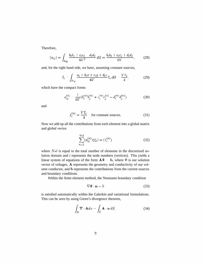
Therefore,(aij) = ZE bibj + cicj + didj6V 2 d = bibj + cicj + didj6V ; (28)

and, for the right hand side, we have, assuming constant sources,Ii = ZE ai + bix+ ciy + diz6V Iv d = V Iv4 : (29)

which have the compact formsa(n)ij = 16V (b(n)i b(n)j + c(n)i c(n)j + d(n)i d(n)j ) (30)

and I(n)i = V Iv4 for constant sources. (31)

Now we add up all the contributions from each element into a global matrixand global vector. NelXn=1(a(n)ij )(�i) = (I(n)i ) (32)

whereNel is equal to the total number of elements in the discretized so-lution domain andi represents the node numbers (vertices). This yields alinear system of equations of the formA� = b, where� is our solutionvector of voltages,A represents the geometry and conductivity of our vol-ume conductor, andb represents the contributions from the current sourcesand boundary conditions.

Within the finite element method, the Neumann boundary conditionr� � n = 0 (33)

is satisfied automatically within the Galerkin and variational formulations.This can be seen by using Green’s divergence theorem,Zr �Adx = Z�A � n dS; (34)

9

and applying it to the left hand side of the Galerkin finite element formula-tion: Zrv � rw d � Z[ @v@x1 @w@x1 + @v@x2 @w@x2 ] d= Z�[v @w@x1n1 + v @w@x2n2] dS � Z v[@2w@x21 + @2w@x22 ] d= Z� v@w@n dS � Z vr2w d: (35)

If we multiply our original differential equation,r2� = �Iv, by an arbi-trary test function and integrate, we obtain(Iv; v) = �Z(r2�)v d = �Z� @�@n v dS + Zr� � rv d = a(�; v);

(36)

where the boundary integral term,@�@n vanishes and we obtain the standardGalerkin finite element formulation.

To apply the Dirichlet condition, we have to work a bit harder. Toapply the Dirichlet boundary condition directly, one usually modifies the(aij) matrix andbi vector such that one can use standard linear systemsolvers. This is accomplished by implementing the following steps.

Assuming we know theith value ofui,1. Subtract from theith member of the r.h.s. the product ofaij and the

known value of�i (call it ��i, this yields the new right hand side,bi = bi � aij ��j.2. Zero theith row and column ofA: aij = aji = 0.

3. Assignaii = 1.

4. Set thejth member of the r.h.s. equal to��i.5. Continue for each Dirichlet condition.

6. Solve the augmented system,A� = bv.3.1.2 Applications of the FE Method for 2-D Domains

Since we show initial results within two-dimensional domains, we brieflycomment on the reduction of the three-dimensional case for tetrahedra tothe two-dimensional case for triangles.

10

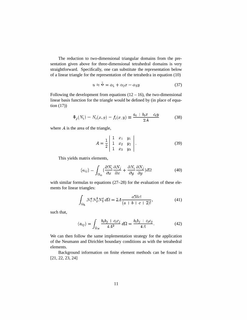
The reduction to two-dimensional triangular domains from the pre-sentation given above for three-dimensional tetrahedral domains is verystraightforward. Specifically, one can substitute the representation belowof a linear triangle for the representation of the tetrahedra in equation (10)u � ~� = �1 + �2x+ �3y (37)

Following the development from equations (12 – 16), the two-dimensionallinear basis function for the triangle would be defined by (inplace of equa-tion (17)) �j(Ni) = Ni(x; y) = fi(x; y) � ai + bix+ ciy2A (38)

whereA is the area of the triangle,A = 12 ������ 1 x1 y11 x2 y21 x3 y3 ������ : (39)

This yields matrix elements,(aij) = ZE (@Ni@x @Nj@x + @Ni@y @Nj@y )d (40)

with similar formulas to equations (27–28) for the evaluation of these ele-ments for linear triangles:Zh Na1N b2N c3 d = 2A a!b!c!(a+ b+ c+ 2)! ; (41)

such that, (aij) = ZE bibj + cicj4A2 d = bibj + cicj4A : (42)

We can then follow the same implementation strategy for the applicationof the Neumann and Dirichlet boundary conditions as with thetetrahedralelements.

Background information on finite element methods can be found in[21, 22, 23, 24]

11

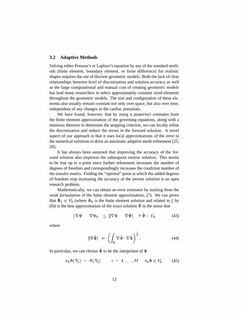
3.2 Adaptive Methods

Solving either Poisson’s or Laplace’s equation by any of thestandard meth-ods (finite element, boundary element, or finite difference)for realisticshapes requires the use of discrete geometric models. Both the lack of clearrelationships between level of discretization and solution accuracy as wellas the large computational and manual cost of creating geometric modelshas lead many researchers to select approximately constantsized elementsthroughout the geometric models. The size and configurationof these ele-ments also usually remain constant not only over space, but also over time,independent of any changes in the cardiac potentials.

We have found, however, that by usinga posteriori estimates fromthe finite element approximation of the governing equations, along with aminimax theorem to determine the stopping criterion, we canlocally refinethe discretization and reduce the errors in the forward solution. A novelaspect of our approach is that it uses local approximations of the error inthe numerical solutions to drive an automatic adaptive meshrefinement [25,26].

It has always been assumed that improving the accuracy of thefor-ward solution also improves the subsequent inverse solution. This seemsto be true up to a point since further refinement increases thenumber ofdegrees of freedom and correspondingly increases the condition number ofthe transfer matrix. Finding the “optimal” point at which the added degreesof freedom stop increasing the accuracy of the inverse solution is an openresearch problem.

Mathematically, we can obtain an error estimator by starting from theweak formulationof the finite element approximation, (7). We can provethat�h 2 Vh (where�h is the finite element solution and related to� by(8)) is the best approximation of the exact solution� in the sense thatkr� � r�hk � kr� � r~�k 8 ~� 2 Vh (43)

where kr~�k = �Zr~� � r~�� 12 : (44)

In particular, we can choose~� to be the interpolant of��h�(Ni) = �(Ni) i = 1; : : : ;M �h� 2 Vh: (45)

12

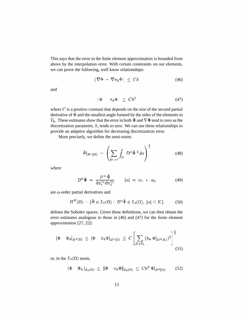
This says that the error in the finite element approximation is bounded fromabove by the interpolation error. With certain constraintson our elements,we can prove the following, well know relationships:kr� � r�h�k � Ch (46)

and k� � �h�k � Ch2 (47)

whereC is a positive constant that depends on the size of the second partialderivative of� and the smallest angle formed by the sides of the elements inVh. These estimates show that the error in both� andr� tend to zero as thediscretization parameter,h, tends to zero. We can use these relationships toprovide an adaptive algorithm for decreasing discretization error.

More precisely, we define the semi-norm:j~�jHr() = 0@Xj�j=r Z jD� ~�j2 dx1A 12(48)

where D� ~� = @j�j ~�@x�11 @x�22 j�j = �1 + �2 (49)

are�-order partial derivatives andHK() = f~� 2 L2() : D� ~� 2 L2(); j�j � Kg (50)

defines the Sobolev spaces. Given these definitions, we can then obtain theerror estimates analogous to those in (46) and (47) for the finite elementapproximation [27, 22]:j�� �hjH1() � j�� �h�jH1() � C " XK2Tn(hkj�jH2(K))2# 12

(51)

or, in theL2() norm,k�� �hkL2() � k�� �h�kL2() � Ch2j�jH2(): (52)

13

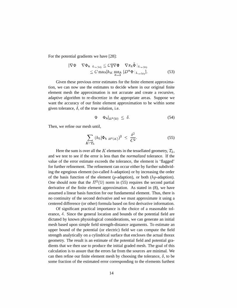
For the potential gradients we have [28]:kr��r�hkL1() � Ckr��r�h~�kL1()� Cmax[hK max�=2 kD��kL1() ]: (53)

Given these previous error estimates for the finite element approxima-tion, we can now use the estimates to decide where in our original finiteelement mesh the approximation is not accurate and create a recursive,adaptive algorithm to re-discretize in the appropriate areas. Suppose wewant the accuracy of our finite element approximation to be within somegiven tolerance,�, of the true solution, i.e.j�� �hjH1() � �: (54)

Then, we refine our mesh until,XK2Th(hkj�hjH2(K))2 � �2C2 : (55)

Here the sum is over all theK elements in the tessellated geometry,Th,and we test to see if the error is less than thenormalizedtolerance. If thevalue of the error estimate exceeds the tolerance, the element is ‘flagged’for further refinement. The refinement can occur either by further subdivid-ing the egregious element (so-calledh-adaption) or by increasing the orderof the basis function of the element (p-adaption), or both (hp-adaption).One should note that theH2() norm in (55) requires the second partialderivative of the finite element approximation. As stated in(8), we haveassumed a linear basis function for our fundamental element. Thus, there isno continuity of the second derivative and we must approximate it using acentered difference (or other) formula based on first derivative information.

Of significant practical importance is the choice of a reasonable tol-erance,�. Since the general location and bounds of the potential fieldaredictated by known physiological considerations, we can generate an initialmesh based upon simple field strength-distance arguments. To estimate anupper bound of the potential (or electric) field we can compute the fieldstrength analytically on a cylindrical surface that encloses the actual thoraxgeometry. The result is an estimate of the potential field andpotential gra-dients that we then use to produce the initial graded mesh. The goal of thiscalculation is to assure that the errors far from the sourcesare minimal. Wecan then refine our finite element mesh by choosing the tolerance,�, to besome fraction of the estimated error corresponding to the elements furthest

14

from the sources. Thus we have used a minimax principle, minimizing themaximum error based upon initial (conservative) estimatesof the potentialfield and potential gradients [25].

3.2.1 Adaptive hp Methods

While Szabo pioneered the method ofhp adaptive finite element methodsin the early 1970s, and their use is widespread among the computationalfluid dynamics and solid mechanics communities, the use of such methodshave basically been non-existent within the bioelectric field community.One reason for this is probably due to the fact that most earlyhp meth-ods for volumetric domains used systems of structured elements. Giventhe complex geometry of the human torso, such methods were difficult toimplement.

More recently, non-conforming formulations have been developed toallow greater flexibility in handling geometric complexities [29, 30, 31].However, such algorithms could be difficult to implement computationallysince new functions needed to be created for each basis function. Thiswas especially true for three-dimensional geometries thatutilized high or-der basis functions. Within the past few years, however, researchers havedeveloped new computationally efficiently hierarchical bases that lead to abetter conditioning of the stiffness matrix and thus allow for fast iterativealgorithms to be effectively employed in the solution of theresulting linearsystem [32].

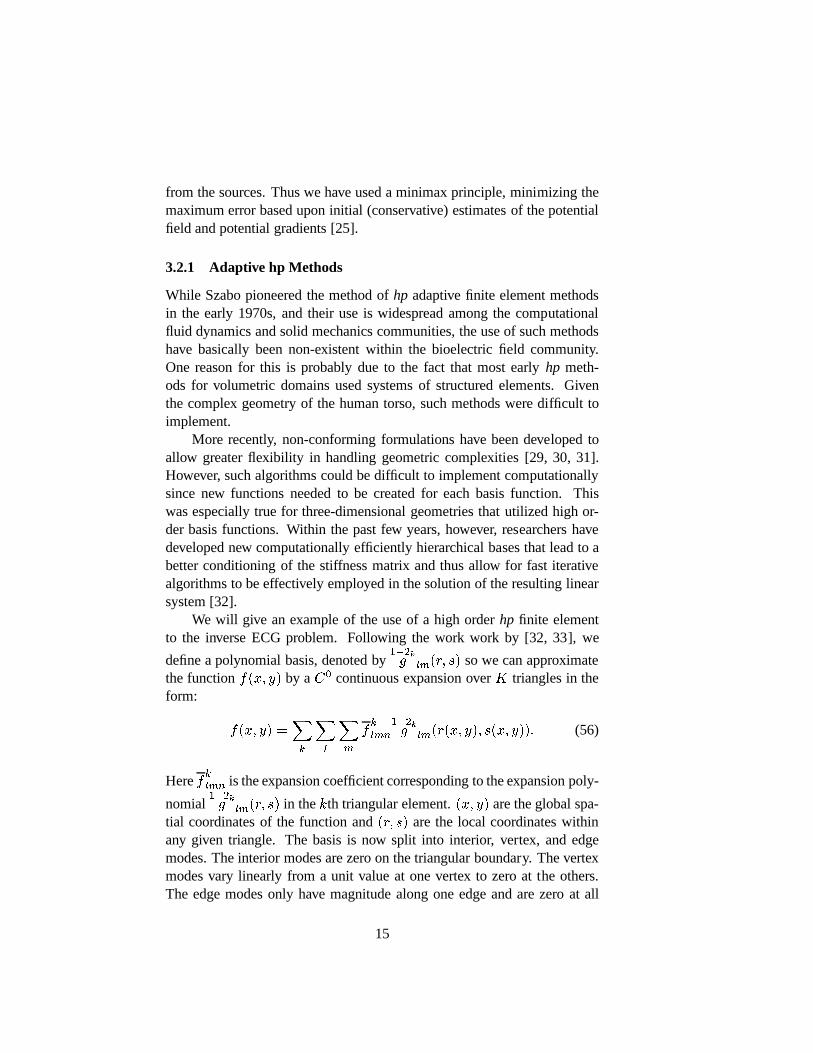
We will give an example of the use of a high orderhp finite elementto the inverse ECG problem. Following the work work by [32, 33], we

define a polynomial basis, denoted by1�2kg lm(r; s) so we can approximate

the functionf(x; y) by aC0 continuous expansion overK triangles in theform: f(x; y) =Xk Xl Xm fklmn1�2kg lm(r(x; y); s(x; y)): (56)

Herefklmn is the expansion coefficient corresponding to the expansionpoly-

nomial1�2kg lm(r; s) in thekth triangular element.(x; y) are the global spa-

tial coordinates of the function and(r; s) are the local coordinates withinany given triangle. The basis is now split into interior, vertex, and edgemodes. The interior modes are zero on the triangular boundary. The vertexmodes vary linearly from a unit value at one vertex to zero at the others.The edge modes only have magnitude along one edge and are zeroat all

15

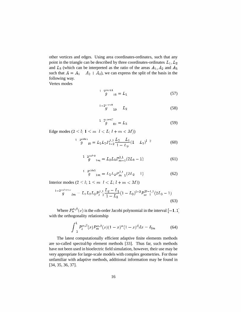
other vertices and edges. Using area coordinates-ordinates, such that anypoint in the triangle can be described by three coordinates-ordinatesL1; L2andL3 (which can be interpreted as the ratio of the areasA1; A2 andA3such thatA = A1 + A2 + A3), we can express the split of the basis in thefollowing way.Vertex modes 1�2vertAg 10 = L1 (57)1�2vertBg 10 = L2 (58)1�2vertCg 01 = L3 (59)

Edge modes (2 � l; 1 � m j l < L; l +m < M))1�2side1g l0 = L1L2P 1;1l�2L2 � L11� L3 (1� L3)l�2 (60)1�2side2g 1m = L2L3P 1;1m�1(2L3 � 1) (61)1�2side3g 1m = L1L3P 1;1m�1(2L3 � 1) (62)

Interior modes (2 � l; 1 � m j l < L; l +m < M))1�2interiorg lm = L1L2L3P 1;1l�2L2 � L11� L3 (1� L3)l�2P 2l�1;1m�1 (2L3 � 1)(63)

WhereP�;�n (x) is thenth-order Jacobi polynomial in the interval[�1; 1]with the orthogonality relationshipZ 1�1 P�;�l (x)P�;�m (x)(1 � x)�(1 + x)�dx = �lm (64)

The latest computationally efficient adaptive finite elements methodsare so-called spectral/hp element methods [33]. Thus far, such methodshave not been used in bioelectric field simulation, however,their use may bevery appropriate for large-scale models with complex geometries. For thoseunfamiliar with adaptive methods, additional informationmay be found in[34, 35, 36, 37].

16

3.3 Regularization

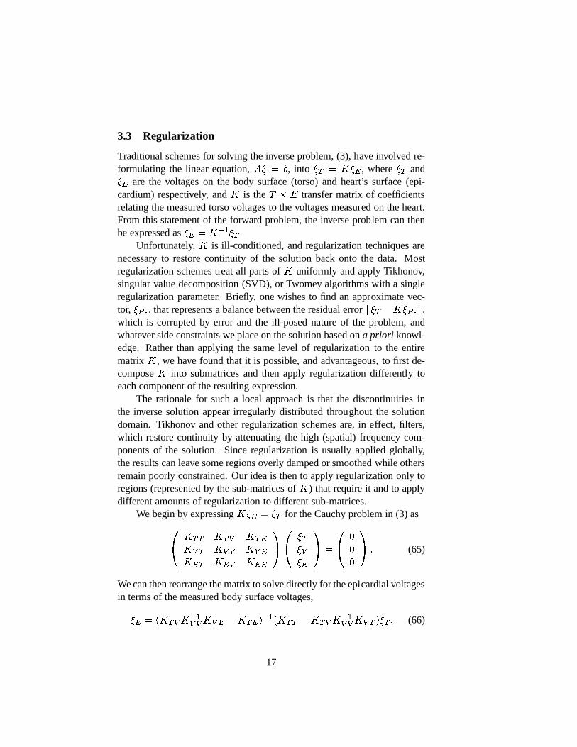
Traditional schemes for solving the inverse problem, (3), have involved re-formulating the linear equation,A� = b, into �T = K�E, where�T and�E are the voltages on the body surface (torso) and heart’s surface (epi-cardium) respectively, andK is theT � E transfer matrix of coefficientsrelating the measured torso voltages to the voltages measured on the heart.From this statement of the forward problem, the inverse problem can thenbe expressed as�E = K�1�T

Unfortunately,K is ill-conditioned, and regularization techniques arenecessary to restore continuity of the solution back onto the data. Mostregularization schemes treat all parts ofK uniformly and apply Tikhonov,singular value decomposition (SVD), or Twomey algorithms with a singleregularization parameter. Briefly, one wishes to find an approximate vec-tor, �E", that represents a balance between the residual errork�T �K�E"k,which is corrupted by error and the ill-posed nature of the problem, andwhatever side constraints we place on the solution based ona priori knowl-edge. Rather than applying the same level of regularizationto the entirematrixK, we have found that it is possible, and advantageous, to firstde-composeK into submatrices and then apply regularization differently toeach component of the resulting expression.

The rationale for such a local approach is that the discontinuities inthe inverse solution appear irregularly distributed throughout the solutiondomain. Tikhonov and other regularization schemes are, in effect, filters,which restore continuity by attenuating the high (spatial)frequency com-ponents of the solution. Since regularization is usually applied globally,the results can leave some regions overly damped or smoothedwhile othersremain poorly constrained. Our idea is then to apply regularization only toregions (represented by the sub-matrices ofK) that require it and to applydifferent amounts of regularization to different sub-matrices.

We begin by expressingK�E = �T for the Cauchy problem in (3) as0@ KTT KTV KTEKV T KV V KV EKET KEV KEE 1A0@ �T�V�E 1A = 0@ 000 1A : (65)

We can then rearrange the matrix to solve directly for the epicardial voltagesin terms of the measured body surface voltages,�E = (KTVK�1V VKV E �KTE)�1(KTT �KTVK�1V VKV T )�T ; (66)

17

where the subscriptsT , V , andE stand for the nodes in the regions of thetorso, the internal volume, and epicardium, respectively.Since torso andepicardial nodes are always separated by more than one element, theKTEsubmatrix is zero, and we can then rewrite (66) as�E = (K�1V EKV VK�1TV )(KTT �KTVK�1V VKV T )�T : (67)

Note that we now have inverses of three sub-matrices,KV E;KTV ,andKV V , as well as several other matrix operations to perform. If oneestimates the condition number,�, of the three sub-matrices using the ratioof the maximum to minimum singular values from a SVD, one findsthat thecondition number varies significantly (from� � 200 for KV V to � � 1 �1016 for KV E in the two-dimensional model described below). Thus, onecan regularize each of the sub-matrices differently, even leaving some of theother sub-matrices untouched. The overall effect of thislocal regularizationis more control over the regularization process.

Since the goal of the inverse problem in electrocardiography is to accu-rately and noninvasively (i.e., non-surgically) estimatethe voltages on theepicardial surface, we need a method to choose ana priori optimal regu-larization parameter. Traditional schemes have been basedon discrepancyprinciples [38], quasi-optimality criterion [38, 39], andgeneralized cross-validation [40]. Recently, Hansen [41] has extended the observations ofLawson and Hanson [42] and proposed a new method for choosingthe reg-ularization parameter based on an algorithm that locates the “corner” of aplot of the norm (or semi-norm) of the side constraint,kLx�k, versus thenorm of the corresponding residual vector,kAx� � bk. In this way, onecan evaluate the compromise between the residual error and the effect ofthe side constraint on the solution. We have utilized thisL-curvealgorithmalong with our local Tikhonov regularization scheme to improve the accu-racy of solutions to the inverse problem.

For the global Tikhonov regularization scheme, we can estimate �E"by minimizing a generalized form of the Tikhonov functional:M�[�E ; ~�T ; ~K] = kK�E � ~�T k2�T + �kC(�E � �0E)k2�E � > 0 (68)

in terms of the epicardial potentials,��E" = [ ~KT ~K + �CTC]�1[ ~KT ~�T + �CTC�0E] (69)

where ~K is the approximation of the true transformation matrix,K, ~�T arethe measured torso potential values,�0E area priori constraints placed on

18

the epicardial potentials based on physiological considerations,C is a con-straint matrix (either the identity matrix, a gradient operator, or a Laplacianoperator), and� is the regularization parameter. For ourlocal regularizationscheme, we replace the global matrix,K, by the two sub-matricesKV E andKTV from (67). We note thatKV V in (67) has a stable inverse and, thus,does not need regularizing.

Another traditional method for regularization the ill-conditioned natureof the transfer matrix is to use a truncated SVD [43]. The singular valuedecomposition of a matrixA is of the formA = U�V T = nXi=1 ui�ivTi ; (70)

whereU = (u1; : : : ; un) 2 Rm�n andV = (v1; : : : ; vn) 2 Rn�n arematrices with orthonormal columns, and where the diagonal matrix, � =diag(�1; : : : ; �n) has non-negative diagonal elements appearing in non-decreasing order and are called the singular values ofA.

Since the condition of the matrixA can be measured (in the 2-norm)in terms of the singular values

cond(A) � kAk2kA�1k2 = �1=�n (71)

one strategy for regularization is to sum the rank-one products of the sin-gular value expansion only to a specified cut-off valuek < n where thesingular value become “small.” For the electrocardiographic inverse prob-lem,K�E = �T , this produces a truncated summation estimate for�E�E = Ky�T = kXi uTi �T�i vi (72)

by projecting the “good” data onto the left and right singular vectorsU andV . While the truncated SVD technique provides answers comparable withTikhonov regularization withL = I, it does not provide optimal results[43].

A related approach that has recently been applied to regularizationof ill-conditioned systems is the generalized singular value decomposi-tion (GSVD) in which the generalized singular values of(A;L) are es-sentially the square roots of the generalized eigenvalues of the matrix pair(ATA;LTL) [16]. The GSVD is a decomposition ofA andL in the formA = U � � 00 In�p �X�1 (73)

19

and L = v(M; 0)X�1 (74)

The columns ofU 2 Rm�n andV 2 Rp�p are orthonormal,X 2 Rn�nis nonsingular with columns that areATA-orthogonal, and� andM arep � p diagonal matrices:� = diag(�1; : : : ; �p), M = diag(�1; : : : ; �p).Thegeneralizedsingular values i of (A;L) are defined as the ratios of�iand�i i = �i�i (75)

The pseudo-inverse ofA in terms of the GSVD can be computed asAy = X � �y 00 In�p �UT (76)

such that a regularized solution can be written as�E = X�� �y 00 In�p �UT �T (77)

where� are called thefilter factorsand depend on the amount of regular-ization. In this case, one would truncate the offending singular values, aswell as modify the basis of the right singular vectors with theL operator.We have found that usingL operators that approximate the operator of theoriginal governing partial differential equation (in thiscase the Laplacian),provide the best results. However, constructing the “best”L operator is stilla topic for further research.

4 Results and Discussion

To study forward and inverse problems in electrocardiography, we devel-oped a series of two- and three-dimensional boundary element and finiteelement models based upon magnetic resonance images from a human sub-ject. Each of 116 MRI scans were segmented into contours defining torso,fat, muscle, lung, and heart regions. Additional node points were added toeach layer and pairs of layers tessellated into tetrahedra using a Delaunaytriangulation algorithm [44, 45] at shown in Figure 1. The resulting modelof the human thorax contained approximately 675,000 volumeelements,each with a corresponding conductivity tensor [46]. A visualization of aforward simulation from epicardial potentials is shown in Figure 2

20

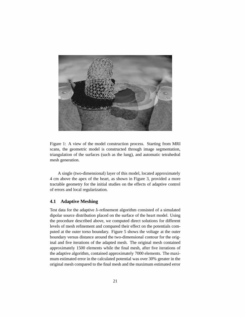
Figure 1: A view of the model construction process. Startingfrom MRIscans, the geometric model is constructed through image segmentation,triangulation of the surfaces (such as the lung), and automatic tetrahedralmesh generation.

A single (two-dimensional) layer of this model, located approximately4 cm above the apex of the heart, as shown in Figure 3, provideda moretractable geometry for the initial studies on the effects ofadaptive controlof errors and local regularization.

4.1 Adaptive Meshing

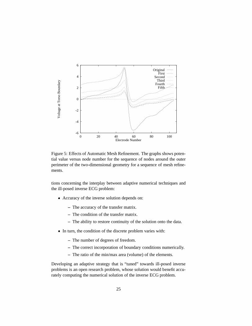
Test data for the adaptiveh-refinement algorithm consisted of a simulateddipolar source distribution placed on the surface of the heart model. Usingthe procedure described above, we computed direct solutions for differentlevels of mesh refinement and compared their effect on the potentials com-puted at the outer torso boundary. Figure 5 shows the voltageat the outerboundary versus distance around the two-dimensional contour for the orig-inal and five iterations of the adapted mesh. The original mesh containedapproximately 1500 elements while the final mesh, after five iterations ofthe adaptive algorithm, contained approximately 7000 elements. The maxi-mum estimated error in the calculated potential was over 30%greater in theoriginal mesh compared to the final mesh and the maximum estimated error

21

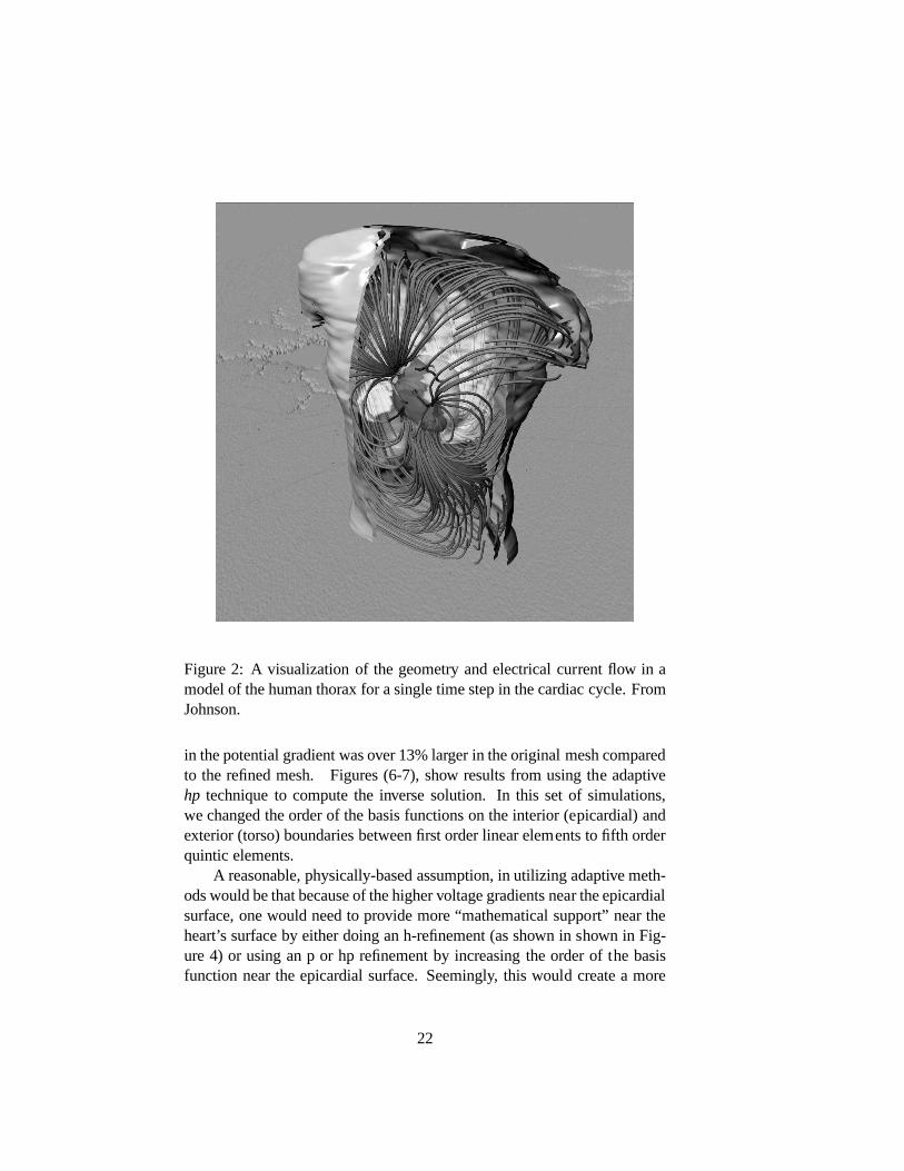
Figure 2: A visualization of the geometry and electrical current flow in amodel of the human thorax for a single time step in the cardiaccycle. FromJohnson.

in the potential gradient was over 13% larger in the originalmesh comparedto the refined mesh. Figures (6-7), show results from using the adaptivehp technique to compute the inverse solution. In this set of simulations,we changed the order of the basis functions on the interior (epicardial) andexterior (torso) boundaries between first order linear elements to fifth orderquintic elements.

A reasonable, physically-based assumption, in utilizing adaptive meth-ods would be that because of the higher voltage gradients near the epicardialsurface, one would need to provide more “mathematical support” near theheart’s surface by either doing an h-refinement (as shown in shown in Fig-ure 4) or using an p or hp refinement by increasing the order of the basisfunction near the epicardial surface. Seemingly, this would create a more

22

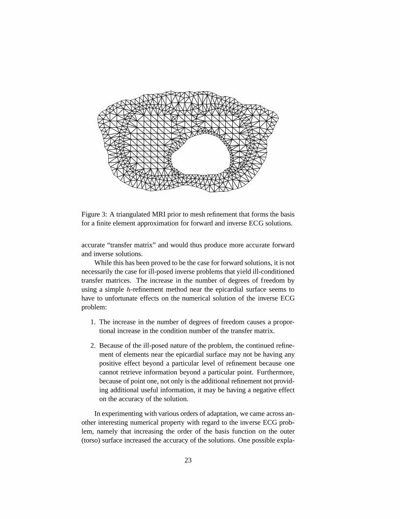
Figure 3: A triangulated MRI prior to mesh refinement that forms the basisfor a finite element approximation for forward and inverse ECG solutions.

accurate “transfer matrix” and would thus produce more accurate forwardand inverse solutions.

While this has been proved to be the case for forward solutions, it is notnecessarily the case for ill-posed inverse problems that yield ill-conditionedtransfer matrices. The increase in the number of degrees of freedom byusing a simpleh-refinement method near the epicardial surface seems tohave to unfortunate effects on the numerical solution of theinverse ECGproblem:

1. The increase in the number of degrees of freedom causes a propor-tional increase in the condition number of the transfer matrix.

2. Because of the ill-posed nature of the problem, the continued refine-ment of elements near the epicardial surface may not be having anypositive effect beyond a particular level of refinement because onecannot retrieve information beyond a particular point. Furthermore,because of point one, not only is the additional refinement not provid-ing additional useful information, it may be having a negative effecton the accuracy of the solution.

In experimenting with various orders of adaptation, we cameacross an-other interesting numerical property with regard to the inverse ECG prob-lem, namely that increasing the order of the basis function on the outer(torso) surface increased the accuracy of the solutions. One possible expla-

23

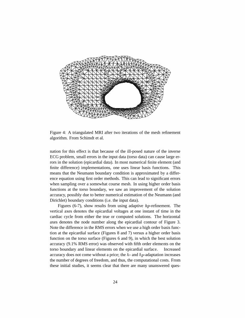
Figure 4: A triangulated MRI after two iterations of the meshrefinementalgorithm. From Schimdt et al.

nation for this effect is that because of the ill-posed nature of the inverseECG problem, small errors in the input data (torso data) can cause large er-rors in the solution (epicardial data). In most numerical finite element (andfinite difference) implementations, one uses linear basis functions. Thismeans that the Neumann boundary condition is approximated by a differ-ence equation using first order methods. This can lead to significant errorswhen sampling over a somewhat course mesh. In using higher order basisfunctions at the torso boundary, we saw an improvement of thesolutionaccuracy, possibly due to better numerical estimation of the Neumann (andDirichlet) boundary conditions (i.e. the input data).

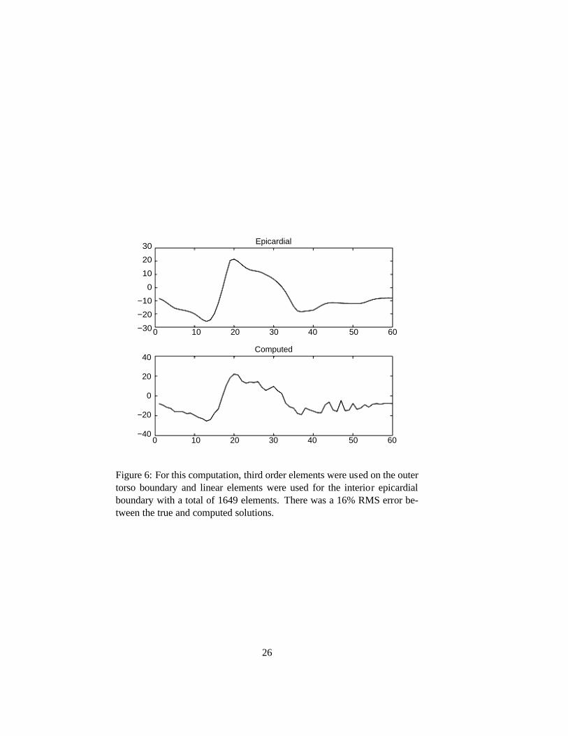
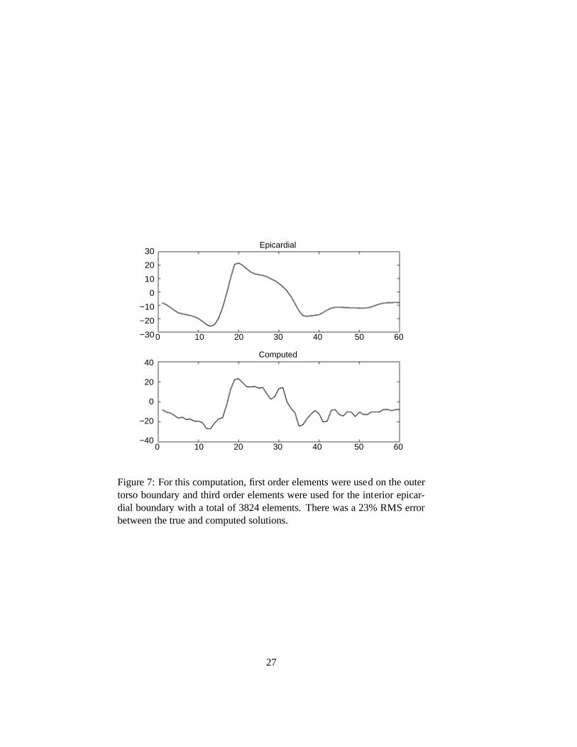
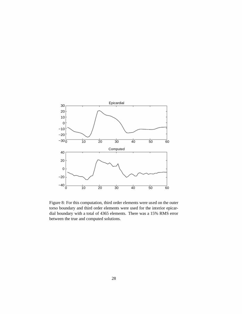
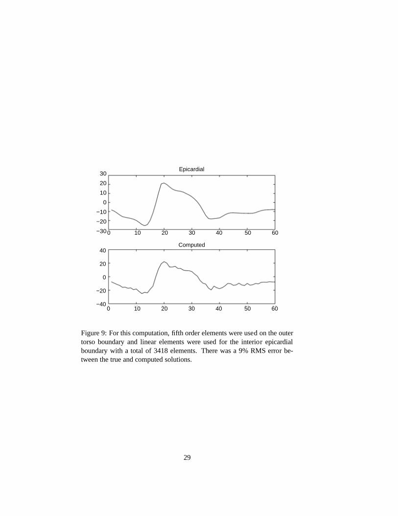
Figures (6-7), show results from using adaptivehp-refinement. Thevertical axes denotes the epicardial voltages at one instant of time in thecardiac cycle from either the true or computed solutions. The horizontalaxes denotes the node number along the epicardial contour ofFigure 3.Note the difference in the RMS errors when we use a high order basis func-tion at the epicardial surface (Figures 8 and 7) versus a higher order basisfunction on the torso surface (Figures 6 and 9), in which the best solutionaccuracy (9.1% RMS error) was observed with fifth order elements on thetorso boundary and linear elements on the epicardial surface. Increasedaccuracy does not come without a price; theh- andhp-adaptation increasesthe number of degrees of freedom, and thus, the computational costs. Fromthese initial studies, it seems clear that there are many unanswered ques-

24

-6

-4

-2

0

2

4

6

0 20 40 60 80 100

Vo

ltag

e a

t T

ors

o B

ou

nd

ary

Electrode Number

OriginalFirst

SecondThird

FourthFifth

Figure 5: Effects of Automatic Mesh Refinement. The graphs shows poten-tial value versus node number for the sequence of nodes around the outerperimeter of the two-dimensional geometry for a sequence ofmesh refine-ments.

tions concerning the interplay between adaptive numericaltechniques andthe ill-posed inverse ECG problem:� Accuracy of the inverse solution depends on:

– The accuracy of the transfer matrix.

– The condition of the transfer matrix.

– The ability to restore continuity of the solution onto the data.� In turn, the condition of the discrete problem varies with:

– The number of degrees of freedom.

– The correct incorporation of boundary conditions numerically.

– The ratio of the min/max area (volume) of the elements.

Developing an adaptive strategy that is “tuned” towards ill-posed inverseproblems is an open research problem, whose solution would benefit accu-rately computing the numerical solution of the inverse ECG problem.

25

0 10 20 30 40 50 60

30

20

10

0

−10

−20

−30

40

20

0

−20

−40

Epicardial

Computed

0 10 20 30 40 50 60

Figure 6: For this computation, third order elements were used on the outertorso boundary and linear elements were used for the interior epicardialboundary with a total of 1649 elements. There was a 16% RMS error be-tween the true and computed solutions.

26

0 10 20 30 40 50 60

30

20

10

0

−10

−20

−30

40

20

0

−20

−40

Epicardial

Computed

0 10 20 30 40 50 60

Figure 7: For this computation, first order elements were used on the outertorso boundary and third order elements were used for the interior epicar-dial boundary with a total of 3824 elements. There was a 23% RMS errorbetween the true and computed solutions.

27

0 10 20 30 40 50 60

30

20

10

0

−10

−20

−30

40

20

0

−20

−40

Epicardial

Computed

0 10 20 30 40 50 60

Figure 8: For this computation, third order elements were used on the outertorso boundary and third order elements were used for the interior epicar-dial boundary with a total of 4365 elements. There was a 15% RMS errorbetween the true and computed solutions.

28

0 10 20 30 40 50 60

30

20

10

0

−10

−20

−30

40

20

0

−20

−40

Epicardial

Computed

0 10 20 30 40 50 60

Figure 9: For this computation, fifth order elements were used on the outertorso boundary and linear elements were used for the interior epicardialboundary with a total of 3418 elements. There was a 9% RMS error be-tween the true and computed solutions.

29

4.2 Local Regularization

To test the local regularization technique, we applied epicardial potentialsrecorded during open chest surgery from a cardiac arrhythmia patient asthe Dirichlet boundary conditions of the two-dimensional model describedabove. The tissue conductivities were assigned as follows:fat = .045 S/m,epicardial fat-pad = .045 S/m, lungs = .096 S/m, skeletal muscle (in the fiberdirection) = .3 S/m, skeletal muscle (across the fiber direction) = .1 S/m,and an average thorax value = .24 S/m. Forward solutions calculated usingthe adapted mesh served as torso boundary conditions, where� = �0 on� � �T for the inverse solution both with and without 10% added Gaussiannoise.

For the sub-matricesAV E andATV , theL-curvealgorithm determinedthe optimala priori regularization parameter. The local Tikhonov regu-larization technique was then applied to the two sub-matrices and the in-verse solution matrix computed. Because the size of the two-dimensionalfinite element model was relatively small, the calculationsstayed in dy-namic memory on an SGI Indigo2 workstation and completed within a fewseconds. To evaluate the results, we compare the locally regularized in-verse solutions to those from a global Tikhonov regularization as well asthe known epicardial solutions.

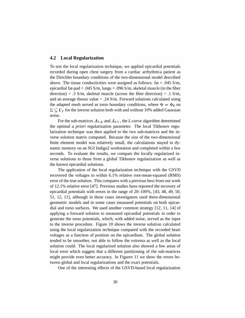
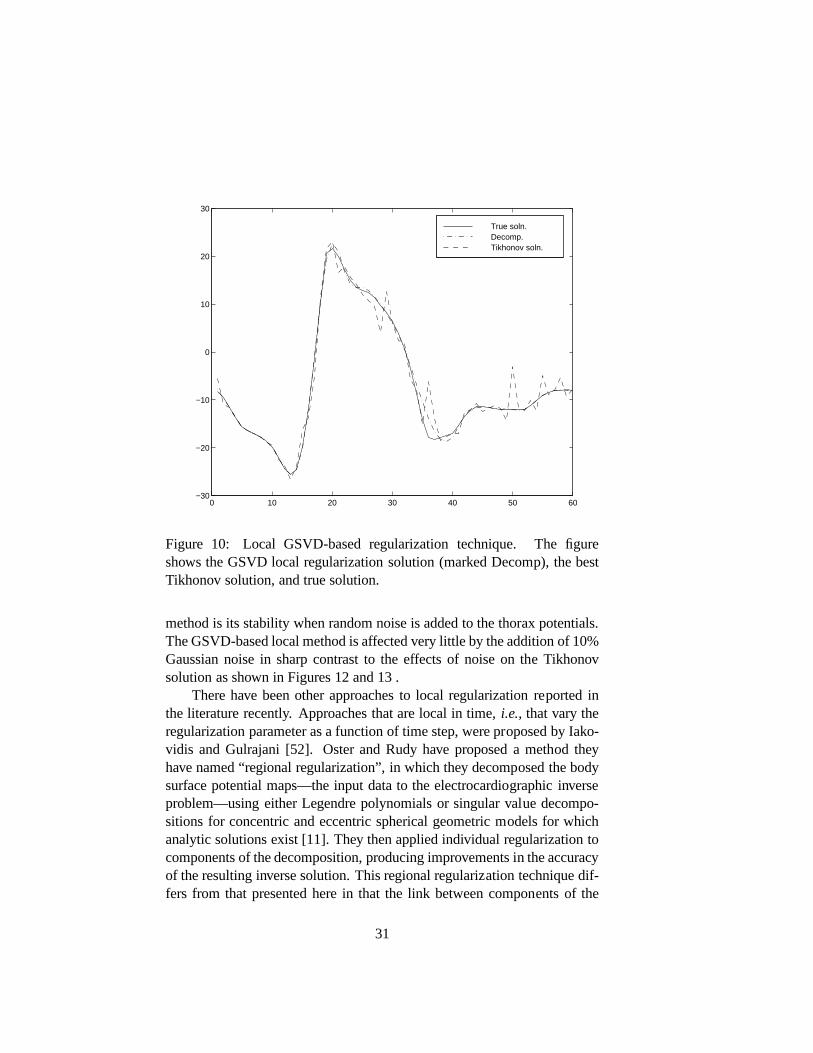
The application of the local regularization technique withthe GSVDrecovered the voltages to within 6.1% relative root-mean-squared (RMS)error of the true solution. This compares with a previous best from our workof 12.1% relative error [47]. Previous studies have reported the recovery ofepicardial potentials with errors in the range of 20–100%, [43, 48, 49, 50,51, 12, 11], although in these cases investigators used three-dimensionalgeometric models and in some cases measured potentials on both epicar-dial and torso surfaces. We used another common strategy [12, 11, 14] ofapplying a forward solution to measured epicardial potentials in order togenerate the torso potentials, which, with added noise, served as the inputto the inverse procedure. Figure 10 shows the inverse solution calculatedusing the local regularization technique compared with therecorded heartvoltages as a function of position on the epicardium. The global solutiontended to be smoother, not able to follow the extrema as well as the localsolution could. The local regularized solution also showeda few areas oflocal error which suggest that a different partitioning of the sub-matricesmight provide even better accuracy. In Figures 11 we show theerrors be-tween global and local regularizations and the exact potentials.

One of the interesting effects of the GSVD-based local regularization

30

0 10 20 30 40 50 60−30

−20

−10

0

10

20

30

True soln. Decomp. Tikhonov soln.

Figure 10: Local GSVD-based regularization technique. Thefigureshows the GSVD local regularization solution (marked Decomp), the bestTikhonov solution, and true solution.

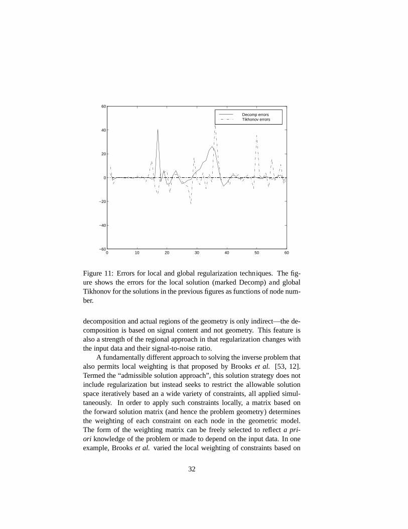
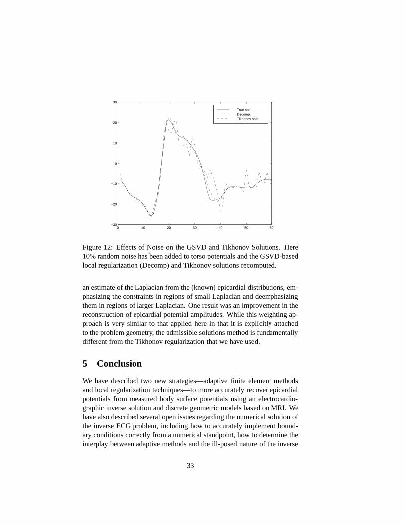
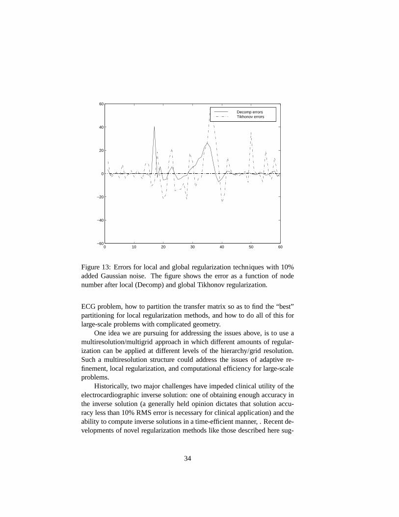
method is its stability when random noise is added to the thorax potentials.The GSVD-based local method is affected very little by the addition of 10%Gaussian noise in sharp contrast to the effects of noise on the Tikhonovsolution as shown in Figures 12 and 13 .

There have been other approaches to local regularization reported inthe literature recently. Approaches that are local in time,i.e., that vary theregularization parameter as a function of time step, were proposed by Iako-vidis and Gulrajani [52]. Oster and Rudy have proposed a method theyhave named “regional regularization”, in which they decomposed the bodysurface potential maps—the input data to the electrocardiographic inverseproblem—using either Legendre polynomials or singular value decompo-sitions for concentric and eccentric spherical geometric models for whichanalytic solutions exist [11]. They then applied individual regularization tocomponents of the decomposition, producing improvements in the accuracyof the resulting inverse solution. This regional regularization technique dif-fers from that presented here in that the link between components of the

31

0 10 20 30 40 50 60−60

−40

−20

0

20

40

60

Decomp errors Tikhonov errors

Figure 11: Errors for local and global regularization techniques. The fig-ure shows the errors for the local solution (marked Decomp) and globalTikhonov for the solutions in the previous figures as functions of node num-ber.

decomposition and actual regions of the geometry is only indirect—the de-composition is based on signal content and not geometry. This feature isalso a strength of the regional approach in that regularization changes withthe input data and their signal-to-noise ratio.

A fundamentally different approach to solving the inverse problem thatalso permits local weighting is that proposed by Brookset al. [53, 12].Termed the “admissible solution approach”, this solution strategy does notinclude regularization but instead seeks to restrict the allowable solutionspace iteratively based an a wide variety of constraints, all applied simul-taneously. In order to apply such constraints locally, a matrix based onthe forward solution matrix (and hence the problem geometry) determinesthe weighting of each constraint on each node in the geometric model.The form of the weighting matrix can be freely selected to reflect a pri-ori knowledge of the problem or made to depend on the input data. In oneexample, Brookset al. varied the local weighting of constraints based on

32

0 10 20 30 40 50 60−30

−20

−10

0

10

20

30

True soln. Decomp. Tikhonov soln.

Figure 12: Effects of Noise on the GSVD and Tikhonov Solutions. Here10% random noise has been added to torso potentials and the GSVD-basedlocal regularization (Decomp) and Tikhonov solutions recomputed.

an estimate of the Laplacian from the (known) epicardial distributions, em-phasizing the constraints in regions of small Laplacian anddeemphasizingthem in regions of larger Laplacian. One result was an improvement in thereconstruction of epicardial potential amplitudes. Whilethis weighting ap-proach is very similar to that applied here in that it is explicitly attachedto the problem geometry, the admissible solutions method isfundamentallydifferent from the Tikhonov regularization that we have used.

5 Conclusion

We have described two new strategies—adaptive finite element methodsand local regularization techniques—to more accurately recover epicardialpotentials from measured body surface potentials using an electrocardio-graphic inverse solution and discrete geometric models based on MRI. Wehave also described several open issues regarding the numerical solution ofthe inverse ECG problem, including how to accurately implement bound-ary conditions correctly from a numerical standpoint, how to determine theinterplay between adaptive methods and the ill-posed nature of the inverse

33

0 10 20 30 40 50 60−60

−40

−20

0

20

40

60

Decomp errors Tikhonov errors

Figure 13: Errors for local and global regularization techniques with 10%added Gaussian noise. The figure shows the error as a functionof nodenumber after local (Decomp) and global Tikhonov regularization.

ECG problem, how to partition the transfer matrix so as to findthe “best”partitioning for local regularization methods, and how to do all of this forlarge-scale problems with complicated geometry.

One idea we are pursuing for addressing the issues above, is to use amultiresolution/multigrid approach in which different amounts of regular-ization can be applied at different levels of the hierarchy/grid resolution.Such a multiresolution structure could address the issues of adaptive re-finement, local regularization, and computational efficiency for large-scaleproblems.

Historically, two major challenges have impeded clinical utility of theelectrocardiographic inverse solution: one of obtaining enough accuracy inthe inverse solution (a generally held opinion dictates that solution accu-racy less than 10% RMS error is necessary for clinical application) and theability to compute inverse solutions in a time-efficient manner, . Recent de-velopments of novel regularization methods like those described here sug-

34

gest that major breakthroughs in numerical accuracy are within our reach.This combination will, we believe, soon lead to practical inverse solutionsin medicine.

We are now pursuing the application of these methods to detailed,large-scale MRI-based thorax models, as well as head/brainmodels forelectroencephalographic inverse problems.

6 Acknowledgments

This research was supported in part by awards from the National ScienceFoundation. The author would like to acknowledge Robert MacLeod’s sig-nificant contribution to this work. Thanks also to Yarden Livnat for assis-tance with thehp finite element simulations and to David Weinstein forhelpful comments and suggestions and help with the figures.

35

References

[1] R.M. Gulrajani, P. Savard, and F.A. Roberge. The inverseproblem inelectrocardiography: Solutions in terms of equivalent sources. Crit.Rev. Biomed. Eng., 16:171–214, 1988.

[2] Y. Yamashita. Theoretical studies on the inverse problem in electro-cardiography and the uniqueness of the solution.IEEE Trans Biomed.Eng., BME-29:719–725, 1982.

[3] J.J.M. Cuppen. Calculating the isochrones of ventricular depolariza-tion. SIAM J. Sci. Statist. Comp., 5:105–120, 1984.

[4] G.J. Huiskamp and A. van Oosterom. The depolarization sequenceof the human heart surface computed from measured body surfacepotentials.IEEE Trans Biomed. Eng., BME-35:1047–1059, 1989.

[5] G.J. Huiskamp and A. van Oosterom. Tailored versus geometry in theinverse problem of electrocardiography.IEEE Trans Biomed. Eng.,BME-36:827–835, 1989.

[6] Y. Rudy and B.J. Messinger-Rapport. The inverse solution in electro-cardiography: Solutions in terms of epicardial potentials. Crit. Rev.Biomed. Eng., 16:215–268, 1988.

[7] R.M. Gulrajani, F.A. Roberge, and G.E. Mailloux. The forward prob-lem of electrocardiography. In P.W. Macfarlane and T.D. VeitchLawrie, editors,Comprehensive Electrocardiology, pages 197–236.Pergamon Press, Oxford, England, 1989.

[8] R.M. Gulrajani, F.A. Roberge, and P. Savard. The inverseproblemof electrocardiography. In P.W. Macfarlane and T.D. VeitchLawrie,editors,Comprehensive Electrocardiology, pages 237–288. PergamonPress, Oxford, England, 1989.

[9] I. Iakovidis and C.F. Martin. A model study of instability of theinverse problem of electrocardiography.Mathematical Biosciences,107:127–148, 1991.

[10] C.R. Johnson and R.S. MacLeod. Local regularization and adaptivemethods for the inverse Laplace problem. In D.N. Ghista, editor,Biomedical and Life Physics, pages 224–234. Vieweg-Verlag, Braun-schweig, 1996.

36

[11] H.S. Oster and Y. Rudy. Regional regularization of the electrocar-diographic inverse problem: A model study using spherical geometry.IEEE Trans Biomed. Eng., 44(2):188–199, 1997.

[12] G.F. Ahmad, D. H Brooks, and R.S. MacLeod. An admissiblesolu-tion approach to inverse electrocardiography.Annal. Biomed. Eng.,26:278–292, 1998.

[13] D.H. Brooks, G. Ahmad, and R.S. MacLeod. Multiply constrainedinverse electrocardiology: Combining temporal, multiplespatial, anditerative regularization. InProceedings of the IEEE Engineering inMedicine and Biology Society 16th Annual International Conference,pages 137–138. IEEE Computer Society, 1994.

[14] D.H. Brooks, G.F. Ahmad, R.S. MacLeod, and G.M. Maratos. In-verse electrocardiography by simultaneous imposition of multipleconstraints.IEEE Trans Biomed. Eng., 46(1):3–18, 1999.

[15] P.C. Hansen. Analysis of discrete ill-posed problems by means of theL-curve. SIAM Review, 34(4):561–580, 1992.

[16] P.C. Hansen.Rank-Deficient and Discrete Ill-Posed Problems: Nu-merical aspects of linear inversion. PhD thesis, Technical Universityof Denmark, 1996.

[17] R.S. MacLeod and D.H. Brooks. Recent progress in inverse prob-lems in electrocardiology.IEEE Eng. in Med. & Biol. Soc. Magazine,17(1):73–83, January 1998.

[18] R.S. MacLeod, R.M. Miller, M.J. Gardner, and B.M. Horacek. Appli-cation of an electrocardiographic inverse solution to localize myocar-dial ischemia during percutaneous transluminal coronary angioplasty.J. Cardiovasc. Electrophysiol., 6:2–18, 1995.

[19] H.S. Oster, B. Taccardi, R.L. Lux, P.R. Ershler, and Y. Rudy. Non-invasive electrocardiographic imaging: Reconstruction of epicardialpotentials, electrograms, and isochrones and localization of single andmultiple electrocardiac events.Circ., 96(3):1012–1024, 1997.

[20] C.J. Penney, J.C. Clements, M.J. Gardner, L. Sterns, and B.M.Horacek. The inverse problem of electrocardiography: applicationto localization of Wolff-Parkinson-White pre-excitationsites. InPro-ceedings of the IEEE Engineering in Medicine and Biology Society

37

17th Annual International Conference, pages 215–216. IEEE Press,1995.

[21] D.S. Burnett. Finite Element Method. Addison Wesley, Reading,Mass., 1988.

[22] C. Johnson.Numerical solution of Partial Differential Equations bythe Finite Element Method. Cambridge University Press, Cambridge,1990.

[23] G. Strang and G. Fix.An Analysis of the Finite Element Method.Prentice–Hall, Englewood Cliffs, NJ, 1973.

[24] B. Szabo and I. Babuska.Finite Element Analysis. John Wiley &Sons, New York, 1991.

[25] C.R. Johnson and R.S. MacLeod. Nonuniform spatial meshadapta-tion using a posteriori error estimates: applications to forward and in-verse problems.Applied Numerical Mathematics, 14:311–326, 1994.

[26] J.A. Schmidt, C.R. Johnson, J.C. Eason, and R.S. MacLeod. Appli-cations of automatic mesh generation and adaptive methods in com-putational medicine. In I. Babuska, J.E. Flaherty, W.D. Henshaw,J.E. Hopcroft, J.E. Oliger, and T. Tezduyar, editors,Modeling, MeshGeneration, and Adaptive Methods for Partial DifferentialEquations,pages 367–390. Springer-Verlag, 1995.

[27] P.G. Ciarlet and J.L Lions.Handbook of Numerical Analysis: FiniteElement Methods, volume 1. North-Holland, Amsterdam, 1991.

[28] R. Rannacher and R. Scott. Some optimal error estimatesfor piece-wise linear finite element approximations.Math. Comp., 38:437–445,1982.

[29] L. Demkowicz, J.T. Oden, W. Rachowicz, and O. Hardy. Towarda universal h-p adaptive finite element strategy, Part 1. Constrainedapproximation and data structure.Computaitonal Methods in AppliedMechanical Engineering, 77:79, 1989.

[30] J.T. Oden, L. Demkowicz, W. Rachowicz, and O. Hardy. Towarda universal h-p adaptive finite element strategy, Part 2. A posteriorierror estimation.Computaitonal Methods in Applied Mechanical En-gineering, 77:113, 1989.

38

[31] W. Rachowicz, J.T. Oden, and L. Demkowicz. Toward a universalh-p adaptive finite element strategy, Part 3. Design of h-p meshes.Computaitonal Methods in Applied Mechanical Engineering, 77:181,1989.

[32] S.P. Sherwin and E.M. Karniakakis. A new triangular andtetrahedralbasis for high-order (hp) finite element methods.International Jour-nal for Numerical Methods in Engineering, 38:3775–3802, 1995.

[33] E.M. Karniakakis and S.P. Sherwin.Spectral/hp Element Methods forCFD. Oxford University Press, Oxford, UK, 1999.

[34] J.E. Flaherty. Adaptive Methods for Partial Differential Equations.SIAM, Philadelphia, 1989.

[35] O.C. Zienkiewicz and J.Z. Zhu. A simple error estimate and adaptiveprocedure for practical engineering analysis.Int. J. Num. Meth. Eng.,24:337–357, 1987.

[36] O.C. Zienkiewicz and J.Z. Zhu. Adaptivity and mesh generation. Int.J. Num. Meth. Eng., 32:783–810, 1991.

[37] I. Babuska. Error bounds for the finite element method.Numer. Math.,16:322–333, 1971.

[38] V.A. Morozov. Methods for Solving Incorrectly Posed Problems.Springer-Verlag, New York, 1984.

[39] R. Kress. Linear Integral Equations. Springer-Verlag, New York,1989.

[40] G.H. Golub, M.T. Heath, and G. Wahba. Generalized cross-validationas a method for choosing a good ridge parameter.Technometrics,21:215–223, 1979.

[41] P.C. Hansen. Analysis of discrete ill-posed problems by means of theL-curve. SIAM Review, 34(4):561–580, 1992.

[42] C.L. Lawson and R.J. Hanson.Solving Least Squares Problems.Prentice-Hall, Englewood Cliffs, NJ, 1974.

[43] R.D. Throne, L.G. Olson, T.J. Hrabik, and J.R. Windle. Generalizedeigensystem techniques for the inverse problem of electrocardiogra-phy applied to a realistic heart-torso geometry.IEEE Trans Biomed.Eng., 44(6):447, 1997.

39

[44] C.R. Johnson, R.S. MacLeod, and P.R. Ershler. A computer model forthe study of electrical current flow in the human thorax.Computersin Biology and Medicine, 22(3):305–323, 1992.

[45] C.R. Johnson, R.S. MacLeod, and M.A. Matheson. Computer sim-ulations reveal complexity of electrical activity in the human thorax.Comp. in Physics, 6(3):230–237, May/June 1992.

[46] K.R. Foster and H.P. Schwan. Dielectric properties of tissues andbiological materials: A critical review.Critical Reviews in Biomed.Eng., 17:25–104, 1989.

[47] C.R. Johnson and R.S. MacLeod. Inverse solutions for electric andpotential field imaging. In R.L. Barbour and M.J. Carvlin, editors,Physiological Imaging, Spectroscopy, and Early DetectionDiagnosticMethods, volume 1887, pages 130–139. SPIE, 1993.

[48] P. Colli Franzone, G. Gassaniga, L. Guerri, B. Taccardi, and C. Vigan-otti. Accuracy evaluation in direct and inverse electrocardiology. InP.W. Macfarlane, editor,Progress in Electrocardiography, pages 83–87. Pitman Medical, 1979.

[49] P. Colli Franzone, L. Guerri, S. Tentonia, C. Viganotti, S. Spaggiari,and B. Taccardi. A numerical procedure for solving the inverse prob-lem of electrocardiography. Analysis of the time-space accuracy fromin vitro experimental data.Math. Biosci., 77:353, 1985.

[50] B.J. Messinger-Rapport and Y. Rudy. Regularization ofthe inverseproblem in electrocardiography: A model study.Math. Biosci.,89:79–118, 1988.

[51] P.C. Stanley, T.C. Pilkington, and M.N. Morrow. The effects ofthoracic inhomogeneities on the relationship between epicardial andtorso potentials.IEEE Trans Biomed. Eng., BME-33:273–284, 1986.

[52] I. Iakovidis and R.M. Gulrajani. Regularization of theinverse epicar-dial solution using linearly constrained optimization. InProceedingsof the IEEE Engineering in Medicine and Biology Society 13thAnnualInternational Conference, pages 698–699. IEEE Press, 1991.

[53] G.F. Ahmad, D.H. Brooks, C.A. Jacobson, and R.S. MacLeod. Con-straint evaluation in inverse electrocardiography using convex opti-mization. InProceedings of the IEEE Engineering in Medicine and

40

Biology Society 17th Annual International Conference, pages 209–210. IEEE Press, 1995.

41