Embed Size (px)
Citation preview

ADAPTIVE CRITIC FLIGHT CONTROL FOR A GENERAL AVIATION AIRCRAFT:
SIMULATIONS FOR THE BEECH BONANZA FLY-BY-WIRE TESTBED
A Thesis by
Rajeev Chandramohan
Bachelor of Electronics & Communication Engineering, Bangalore University, 2001
Submitted to the Department of Aerospace Engineering
and the faculty of the Graduate School of
Wichita State University
in partial fulfillment of
the requirements for the degree of
Master of Science
July 2007

© Copyright 2007 by Rajeev Chandramohan
All Rights Reserved
iii
ADAPTIVE CRITIC FLIGHT CONTROL FOR A GENERAL AVIATION AIRCRAFT:
SIMULATIONS FOR THE BEECH BONANZA FLY-BY-WIRE TESTBED
I have examined the final copy of this Thesis for form and content and recommend that it be
accepted in partial fulfillment of the requirement for the degree of Master of Science with a
major in Aerospace Engineering
__________________________________
James E Steck, Committee Chair
We have read this Thesis
and recommend its acceptance:
__________________________________
Kamran Rokhsaz, Committee Member
_________________________________
John Watkins, Committee Member
__________________________________
Silvia Ferrari, Committee Member

iv
ACKNOWLEDGMENTS
I would like to thank my advisor, Dr. James E Steck, for his guidance and support. I
would like to extend my gratitude to the members of my committee, Dr. Kamran Rokhsaz, Dr.
John Watkins and Dr. Silivia Ferrari, for their helpful comments and suggestions. I also want to
thank my family and friends.

v
ABSTRACT
An adaptive and reconfigurable flight control system is developed for a general aviation aircraft.
The flight control system consisting of two neural networks is developed using a two phase
procedure called the pre-training phase and the online training phase. The adaptive critic method
used in this thesis was developed by Ferrari and Stengel. In the pre-training phase the
architecture and initial weights of the neural network are determined based on linear control. A
set of local gains for the linearized model of the plant is obtained at different design points on the
velocity v/s altitude envelope using an LQR method. The pre-training phase guarantees that the
neural network controller meets the performance specifications of the linear controllers at the
design points. Online training uses a dual heuristic adaptive critic architecture that trains the two
networks to meet performance specifications in the presence of nonlinearities and control
failures. The control system developed is implemented for a three-degree-of-freedom
longitudinal aircraft simulation. As observed from the results the adaptive control system meets
performance requirements, specified in terms of the damping ratio of the phugoid and short
period modes, in the presence of nonlinearities. The neural network controller also compensates
for partial elevator and thrust failures. It is also observed that the neural network controller meets
the performance specification for large variations in the parameters of the assumed and actual
models.

vi
TABLE OF CONTENTS
Chapter Page
1. INTRODUCTION .........................................................................................................................................1
1.1 Background....................................................................................................................................................5
1.2 Artificial neural networks..........................................................................................................................9
1.3 Thesis Organization ..................................................................................................................................12
1.4 Summary of results....................................................................................................................................12
2. NEURAL CONTROL DESIGN ..............................................................................................................14
2.1 Performance Measure ...............................................................................................................................15
2.2 Aircraft optimal control problem ..........................................................................................................17
2.2 Linear Quadratic Regulator.....................................................................................................................18
2.3 Nonlinear neural controller .....................................................................................................................25
2.4 Adaptive critic fundamentals..................................................................................................................27
3. ALGEBRAIC TRAINING OF NEURAL NETWORKS.................................................................31
3.1 Exact gradient based solution.................................................................................................................34
4. LINEAR CONTROL DESIGN................................................................................................................38
4.1 Flight envelope ...........................................................................................................................................40
4.2 Linear controller design ...........................................................................................................................43
4.2 Implicit model following .........................................................................................................................46
4.3 Neural network based controller ...........................................................................................................51
4.4 Response of initialized neural network ...............................................................................................55
4.5 Critic neural network ................................................................................................................................57

vii
TABLE OF CONTENTS (Cont.)
Chapter Page
5. ADAPTIVE CRITIC FLIGHT CONTROL .........................................................................................60
5.1 Dual heuristic adaptive critic ..................................................................................................................61
5.2 Action and critic networks ......................................................................................................................61
5.3 Online adaptation .......................................................................................................................................69
6. SIMULATION AND RESULTS ............................................................................................................73
6.1 Simulation ....................................................................................................................................................73
6.2 Results ...........................................................................................................................................................74
7. CONCLUSION.............................................................................................................................................89
REFERENCES .......................................................................................................................................................91

viii
LIST OF FIGURES
Figure Page
Figure 1: Backward dynamic programming for a two stage process.............................................. 7
Figure 2: Approximate dynamic programming .............................................................................. 8
Figure 3: Artificial neuron ............................................................................................................ 10
Figure 4: Single hidden layer neural network............................................................................... 11
Figure 5: Relationship between Cost function and Value function .............................................. 21
Figure 6: Adaptive critic based neural network controller. .......................................................... 25
Figure 7: Sigmoidal neural network. ............................................................................................ 32
Figure 8: Operating envelope........................................................................................................ 39
Figure 9: Flight envelope .............................................................................................................. 42
Figure 11: Neural network based PI controller............................................................................. 51
Figure 12: Initialized feedback neural network architecture ........................................................ 54
Figure 13: Initialized integral neural network architecture........................................................... 55
Figure 14: Response at a design point .......................................................................................... 56
Figure 15: Response at an interpolation point .............................................................................. 57
Figure 16: Initialized critic neural network. ................................................................................. 59
Figure 17: Vector output neural network...................................................................................... 62
Figure 18: Action neural network. ................................................................................................ 66
Figure 19: Critic neural network................................................................................................... 68
Figure 20: Action network adaptation. ......................................................................................... 70
Figure 21: Critic network adaptation. ........................................................................................... 71
Figure 22: Velocity response and throttle setting for partial elevator failure. .............................. 76

ix
LIST OF FIGURES (Cont.)
Figure Page
Figure 23: Flight path angle response and elevator deflection for partial elevator failure. .......... 76
Figure 26: Velocity response and throttle setting for partial thrust failure................................... 78
Figure 27: Flight path angle response and elevator deflection for partial thrust failure............... 78
Figure 28: Angle of attack and pitch angle for partial thrust failure. ........................................... 79
Figure 29: Incremental cost for partial thrust failure. ................................................................... 79
Figure 30: Velocity response and throttle setting for variation inαmC and
qmC . .......................... 80
Figure 31: Flight path angle response and elevator deflection for variation inαmC and
qmC . ...... 81
Figure 32: Angle of attack and pitch angle for variation inαmC and
qmC ..................................... 81
Figure 33: Incremental cost for variation inαmC and
qmC . ........................................................... 82
Figure 34: Flight path angle response and elevator deflection for variation inkDC . .................... 83
Figure 35: Velocity response and throttle setting for variation inkDC . ........................................ 83
Figure 36: Angle of attack and pitch angle for variation inkDC . .................................................. 84
Figure 37: Incremental cost for variation inkDC . ......................................................................... 84
Figure 38: Velocity response and throttle setting for a command of -40 ft/s in velocity. ............ 85
Figure 39: Flight path angle response and elevator deflection for a command of -40 ft/s in
velocity.......................................................................................................................................... 86
Figure 40: Angle of attack and theta time history for a command of -40 ft/s in velocity............. 86
Figure 41: Altitude time history for a command of -40 ft/s in velocity........................................ 87
Figure 42: Incremental cost for a command of -40 ft/s in velocity. ............................................. 87

x
LIST OF TABLES
Table Page
Table 1: Flying qualities for class I aircraft in terminal phase flight.............................................46

xi
LIST OF SYMBOLS
a Scheduling variable
AR Aspect ratio of the wing
b Neural network output bias
C Linear gain matrix
0DC Drag coefficient at zero lift
BC Feedback gain matrix
FC Forward gain matrix
IC Integral gain matrix
LC Lift coefficient
d Neural network input bias
D Total aircraft drag
e Oswalds efficiency factor
F Linear state Jacobian matrix
G Linear control Jacobian matrix
h Aircraft altitude
xH Jacobian matrix of a linear systems output with respect to the state
uH Jacobian matrix of a linear systems output with respect to control
[ ]H • Hamiltonian
J Cost function
*J Optimal cost
[ ]L • Lagrangian
xii
LIST OF SYMBOLS (Cont.)
M Matrix of cross-coupling weighting between the state and control
ANN Action neural network
CNN Critic neural network
p Neural network input vector
P Steady state Riccati matrix
AP Power available
RP Power required
q Aircraft pitch rate
Q State weighting matrix
R Control weighting matrix
S Matrix of sigmoidal functions evaluated at input to node values
S Aircraft wing reference area
t Time variable in continuous-time representation
kt Time variable in sampled-time representation
AT Thrust available
RT Thrust required
u Control signal
0u Trim control signal
u% Control deviation from commanded control
v Neural network output weight vector
V Aircraft velocity

xiii
LIST OF SYMBOLS (Cont.)
[ ]V • Cost-to-go or value function
V∞ Free stream velocity
W Neural network input weight matrix
W Aircraft weight
x State variable
ax Augmented state
cy Command input
y Output state
z Output of neural network
α Angle of attack
Tδ Throttle position
eδ Elevator deflection
()∆ Perturbation from the equilibrium value
γ Vertical flight path angle
λ Adjoint vector
θ Aircraft pitch angle
ρ∞ Free stream air density
σ Sigmoid activation function
ξ Time integral of output error

1. INTRODUCTION
Controllers can be designed for systems so as to change the response of the system to
meet performance specifications. Linear control theory provides a basis for designing control
systems to meet performance specifications. One of the major disadvantages of linear control
theory is that the system to be controlled must be modeled by linear ordinary differential
equations. Most systems in practice are highly nonlinear in nature. This renders linear control
system design unsuitable for many practical systems. To overcome this drawback, the systems
are linearized about an operating point and control systems are designed at the operating point
using linear control theory. The control law developed about an operating point deteriorates in
performance for conditions further away from that point due to nonlinearities. This necessitates
the design of a controller that meets performance specifications over its entire operating range.
A fixed controller that meets performance specifications in the presence of differences
between the actual plant and the assumed model is termed to be robust. A controller that varies
its parameters during its operation is termed to be adaptive or gain scheduled. An adaptive
controller can be expected to perform better in the presence of uncertainty than a fixed controller.
A controller that can meet performance specifications in the presence of system failure is said to
be reconfigurable.
The objective of this thesis was to develop an adaptive control system that is both robust and
reconfigurable for a general aviation aircraft that is modeled by nonlinear ordinary differential
equations. The adaptive controller is developed using neural networks in conjunction with linear
control theory. The proposed control system would render the aircraft easier to fly, even for
pilots with relatively low piloting skills. The controller adapts and reduces pilot workload in the
presence of partial control failures making it safer to fly the aircraft.

2
The application of neural networks for the control of nonlinear systems has been studied
extensively in the past by various authors. Several different schemes using neural networks for
control have been investigated, these include the inverse controller architecture using neural
networks, dynamic inversion neural network control and adaptive critic based neural network
control. In addition the areas of application of neural networks for control studied include
robotics, chemical plant control, and vehicle control among others. Neural network control of
aircraft have also been studied extensively in the past using different control architectures.
Suresh et al. [1] have developed a neural network (NN) based control system to improve
damping and follow piloted input commands for the F-8 fighter aircraft. The controller is used to
approximate the control law derived using linear system theory. The NN controller is trained
offline using a reference model of the aircraft and online the NN adapts for variations in
aerodynamic stability derivatives and control derivatives.
Calise et al. [2] have developed a direct adaptive tracking controller based on neural
networks. The neural networks were used to represent the nonlinear inverse transformation for
feedback linearization. In this method the neural networks were trained offline using a nominal
mathematical model of the F-18 high performance aircraft. The neural networks are then trained
online to compensate for the modeling errors between the actual and nominal mathematical
model.
Rysdyk et al. [3] have used a neural network augmented dynamic model inversion control for
a civilian rotorcraft. They use neural networks to account for nonlinearities and modeling error
between the actual plant and an inverse controller. One of the main advantages of the scheme
proposed by the authors is that there is no need for off-line training as all the information
available is incorporated in the design of the inverse controller. The above scheme is

3
implemented for attitude hold and attitude command in the longitudinal channel. The proposed
system provides consistent response over the entire flight envelope of the tiltrotor including in
transition flight.
Perhinschi et al. [4] have used a neural network augmented dynamic inversion model control
for the F-15 high performance aircraft. In addition they use a neural network that is trained
offline to provide the aerodynamic and control stability derivatives. They have shown that when
the offline neural network is adapted online the compensating signal of the neural network used
to remove dynamic inversion reduces.
Burlet et al. [5] have developed a neural network based adaptive controller based on linear
programming and adaptive critic techniques for a simulated C-17 aircraft. Linear programming
techniques have been used to allocate the control deflections generated in the presence of failures
in an optimal manner. The adaptive critic is used to update the parameters of the reference model
to provide consistent handling qualities. Piloted simulations of the controller were carried out to
asses the performance of the controller in the presence of simulated failure conditions.
Steck et al. [6] have implemented a neural network augmented dynamic model inversion
control for general aviation aircraft control. They have also investigated the performance of the
control scheme in the presence of turbulence [7] as well as microburst [8]. The authors have also
presented pilot evaluation of the controller using flight simulation. The control scheme
developed was shown to be able to follow piloted commands even in the presence of
unanticipated failures in the system.
Kulkarni et al. [9] have developed a neural network based methodology for the design of
optimal controllers for nonlinear system. The system consists of two neural networks: one
predicts the cost to go from the present state; the second neural network is trained to minimize

4
the output of the first neural network. Since the second network minimizes the output of the first
neural network it converges to the optimal solution and can be used as an optimal controller.
Balakrishnan et al. [10] have studied extensively the application of adaptive critic for aircraft
optimal control. The adaptive critic controller is evaluated for the longitudinal control of an
aircraft and is seen to provide near optimal control policies for the control of the aircraft. In
another work Balakrishnan et al. [11] have designed an adaptive critic based autolanding
controller for aircraft. The performance of the adaptive critic based controller is compared with
that of a classical PID controller.
Shin et al. [12] have demonstrated the use of a neural network based adaptive output
feedback control for an F-15 aircraft at high angles of attack. The method utilizes a fixed gain
linear controller in combination with a neural network to compensate for model inversion error.
The linear controller is designed using output feedback linearization. The total control input to
the aircraft is the sum of the linear controller output and the output of the neural network which
compensates for the modeling error between the actual and assumed dynamics at high angles of
attack.
Williams-Hayes [13] with the intelligent flight control system project team has developed a
neural network based adaptive controller for a highly modified F-15B aircraft. The neural
network based adaptive controller is used to optimize aircraft performance and also to
compensate for unknown failures during flight. Simulations of the experiments to be performed
in the flight test are used to evaluate the performance of the adaptive controller.
Ferrari et al. [14] have proposed a novel scheme for classical neural synthesis for control
of non linear systems. In this scheme the initialization of the neural networks is based on linear
control theory. The parameters for the neural networks are obtained by designing linear control

5
gains for a set of linear models covering the entire operating range of the aircraft using LQR
methods. The initialized neural networks are then adapted online using adaptive critic method to
improve performance based on actual system dynamics. They have applied this scheme to the
design of six degree of freedom business jet simulation. The simulations show that the proposed
scheme follows pilot inputs in the presence of parameter variations and unanticipated control
failures. This method is used in this thesis to design an adaptive controller for three degree of
freedom general aviation aircraft control.
The methodology presented in this thesis combines linear control theory and neural
networks to control the nonlinear aircraft dynamics. Gain scheduling is used in the design of the
linear controller as it provides a means of applying linear control laws over the entire envelope of
the aircraft which is widely used in the industry. The initialized controller designed using LQR
method is robust to nonlinearities and model uncertainties. In the online phase the controller
adapts to the actual dynamics of the aircraft and accommodates for a larger degree of uncertainty
than the initialized controller.
1.1 Background
The control of nonlinear systems so as to minimize a cost is one of the fundamental
problems in optimal control theory. The cost J is a measure of the performance of the control
system. A control policy is said to be optimum if the controller minimizes the cost. The cost is a
combination of the physically important states and control signals. There are various kinds of
performance measures for different kinds of problems. Some of the different types of costs are
minimum time problems, terminal control problems, minimum control effort problems, tracking
problems etc. Once the performance measure or cost to be minimized is determined the next task
is to determine a control function that minimizes the cost. It is often useful to find the optimal

6
control policy as a function of the state at any given time t as this can be used to generate the
control based on the state without the need for a lookup table implementation. Two methods
exist for finding the optimal policy functional so as to minimize the cost. These are the principle
of dynamic programming and the minimum principle of Pontryagin. Adaptive critic designs are
based on the principle of dynamic programming.
Dynamic programming uses the principle of optimality to determine the optimal control
policy. The principle of optimality can be explained as follows. The optimal solution to a global
problem is a combination of optimal solutions to all of its constituent sub problems.
Let us now apply the principle of optimality to a two stage process in order to determine the
optimal policy from the initial to the final state. Now if we determine the optimal path from all
the intermediate states to the last state, The principle of optimality states that this path lies on the
globally optimal path from the initial state passing through the intermediate state. Let the optimal
path to the final state f from the intermediate states edc ,, be associated with the optimal
cost *cfJ , *
dfJ , *efJ as shown in the Figure 1. Now by the principle of optimality, the optimal cost
from b to f via each of the intermediate states is given by
**
cfbcbcf JJJ += , **dfbdbdf JJJ += , **
efbebef JJJ += (1)
The overall optimal path from b to f is found by taking the minimum of the above three
values, i.e.
),,min( ****
befbdfbcfbf JJJJ = (2)

7
Figure 1: Backward dynamic programming for a two stage process.
Thus we can find the optimal global path by trying all the local paths, then following the
optimal paths from then on for each of these and choosing the one with minimum cost. For
systems with a large number of states and large number of stages, the above process has to be
repeated backward for each stage and the optimal values stored until we reach the initial stage
from which we can determine the optimal policy to reach the final value from the initial state.
This becomes infeasible for systems with even a relatively few number of states and the number
of computations grows exponentially with the number of states; this is commonly referred to as
the “curse of dimensionality”. The Approximate dynamic programming method uses incremental
optimization combined with a neural network to reduce the computations associated with
evaluating cost at each stage.
In dynamic programming we progress backward in time starting from the final state where as
in approximate dynamic programming [16] we progress forward in time. In approximate
dynamic programming the optimal control policy and the cost associated with it is calculated
*
efJ
*
dfJ
*
cfJ
Jbe
Jbd
Jbc
f
e
d
c
b

8
based on the current state. This can be explained better by considering a two stage process as
shown in Figure 2. At the first stage a , the cost associated with going from a tob , abJ can be
calculated based on the current state and the current control needed to go from a tob . The
optimal cost to go from the state b to the final state is estimated as *ˆbfJ by a parametric structure
that approximates the cost to go based on the current state and control. The path ba − is chosen
to minimize the cost *ˆbfab JJ + . At the next stage, cb − the above procedure is repeated but with
the information available from the previous stage the policy and cost approximations ( *J ) have
had a chance to improve and the next path from fc − is closer to the optimal trajectory.
Figure 2: Approximate dynamic programming
Adaptive critic design is based on approximate dynamic programming and produces the most
general solution of approximate dynamic programming. The importance of adaptive critic design
is that it attempts to overcome the curse of dimensionality by ensuring convergence to the
optimal solution over time. There are three different forms of adaptive critic designs [17]. In the
*ˆbfJ
cfJ
bcJ
abJ
f
c b
a
*ˆcfJ
9
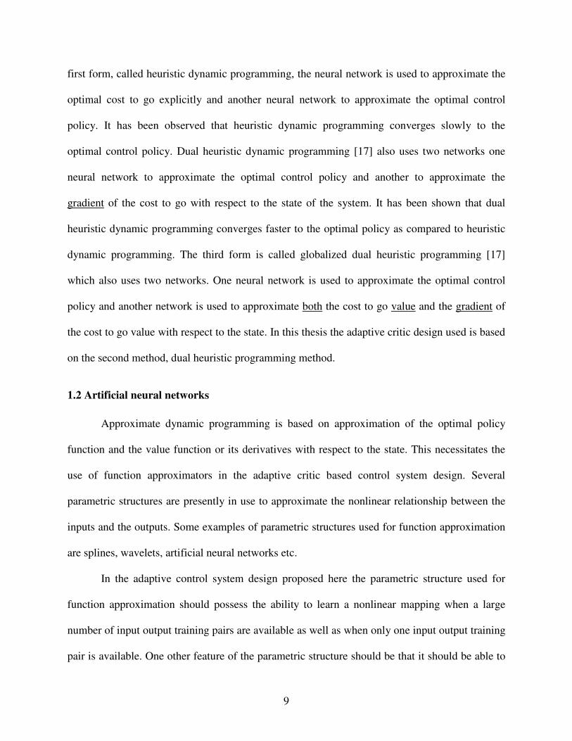
first form, called heuristic dynamic programming, the neural network is used to approximate the
optimal cost to go explicitly and another neural network to approximate the optimal control
policy. It has been observed that heuristic dynamic programming converges slowly to the
optimal control policy. Dual heuristic dynamic programming [17] also uses two networks one
neural network to approximate the optimal control policy and another to approximate the
gradient of the cost to go with respect to the state of the system. It has been shown that dual
heuristic dynamic programming converges faster to the optimal policy as compared to heuristic
dynamic programming. The third form is called globalized dual heuristic programming [17]
which also uses two networks. One neural network is used to approximate the optimal control
policy and another network is used to approximate both the cost to go value and the gradient of
the cost to go value with respect to the state. In this thesis the adaptive critic design used is based
on the second method, dual heuristic programming method.
1.2 Artificial neural networks
Approximate dynamic programming is based on approximation of the optimal policy
function and the value function or its derivatives with respect to the state. This necessitates the
use of function approximators in the adaptive critic based control system design. Several
parametric structures are presently in use to approximate the nonlinear relationship between the
inputs and the outputs. Some examples of parametric structures used for function approximation
are splines, wavelets, artificial neural networks etc.
In the adaptive control system design proposed here the parametric structure used for
function approximation should possess the ability to learn a nonlinear mapping when a large
number of input output training pairs are available as well as when only one input output training
pair is available. One other feature of the parametric structure should be that it should be able to

10
approximate the nonlinear mapping of multidimensional input output space. Of all the parametric
structures which can be used for function approximators only the artificial neural networks have
the above properties.
Artificial neural networks are based on the way biological neurons present in the brain
process information. Artificial neural networks are composed of a large number of processing
elements arranged in the form of layers and connected with each other by a means of
communication links. Each of these communication links has a weight associated with it; the
weights of these communication links are changed in order to approximate the nonlinear
functional relationship between the input and the output. Each neuron also has an internal
process, called the activation function that acts on the net input to the neuron. Some of the
commonly used activation functions are the sigmoid, tanh, linear, radial basis etc. The basic
structure of an artificial neuron is as shown in Figure 3.
Figure 3: Artificial neuron
n
w3
w2
w1
∑
d
Output
1x
2x
3x
σ

11
The neural networks used for the adaptive control system in this thesis, use single hidden
layer neural networks with sigmoidal activation functions as shown in Figure 4. In most neural
network applications the neural networks are trained using supervisory training algorithms. In
supervisory training algorithms the goal is to reduce the error between the actual output of the
neural network and a target output. Backpropogation algorithms have been devised to modify the
weights of the neural network architecture in order to reduce the error. Once the neural networks
output is close to the desired output, the training is stopped and the neural network is said to be
trained. One of the problems associated with the training of neural networks is the problem of
overfitting. Overfitting is characterized by the network having a desired network error for the
training set, but having large errors for input output pairs not present in the training set.
Figure 4: Single hidden layer neural network
In this thesis a backpropogation technique termed modified resilient back propagation
[16] is utilized for training both the action network and the critic network to approximate the
1x
2x
3x
1y
2y
3y
Processing
element
12
optimal policy and the gradient of the cost to go function with respect to the states of the system
in the online training phase. The modified resilient back propagation used for training preserves
the information learned by the neural networks during the initialization phase.
1.3 Thesis Organization
The thesis is organized into six chapters. In this chapter the two phase design of the
nonlinear neural controller is introduced. Chapter two introduces the concept of optimal control
of nonlinear systems using neural networks. Chapter three introduces the concept of algebraic
initialization of neural networks. Chapter four goes into the details of linear control design on
which the nonlinear controller is based. Chapter four also compares the performance of the
initialized neural controller with that of the linear controller operations with the nonlinear aircraft
model. Chapter five gives an explanation of the algorithm used to implement adaptive critic
designs. In chapter six, the neural networks are allowed to adapt online to account for
nonlinearities which were ignored during the linear control designs. The response of the
controller is evaluated using MATLAB simulations of a three degree of freedom general aviation
aircraft in chapter six. The controller performance is evaluated with control failures and
variations between the actual and assumed parameters. Chapter seven derives the conclusion of
the thesis as well as suggests improvements and future work.
1.4 Summary of results
The nonlinear neural network controller is developed using the two stage process outlined
above. The nonlinear neural network controller is tested with the longitudinal nonlinear model of
a general aviation aircraft. The results show that the controller improves performance in the
presence of nonlinearities as compared to the linear controller design based on linearized model

13
of the aircraft. The controller follows pilot inputs even in the presence of unanticipated control
failures preserving stability for the closed loop system. Simulation results show that the
controller preserves stability of the system and follows pilot input commands for large variations
inαmC and
0DC .

14
2. NEURAL CONTROL DESIGN
The determination of an optimal control policy so as to minimize the cost of a metric is
one of the fundamental problems of control theory. There exist closed form solutions for the
determination of an optimal control policy for systems that are linear. Almost all systems of
physical significance exhibit nonlinear behavior. Therefore there is a need for the design of a
control system for a nonlinear plant so as to minimize a cost.
Since there exists much literature for the design of control systems for plants which are
linear, nonlinear plants are linearized about different operating points to obtain a set of linear
models covering the entire operating range. Linear controllers which then satisfy optimality
criteria as well as robustness criteria can be designed for the each of the operating or design
points. This method is followed widely in the industry and is termed gain scheduling. The
controller gains obtained at different operating points for the linearized model are interpolated
based on the operating conditions using a set of significant variables called scheduling variables.
Even the gain scheduled control systems do not always meet performance specifications
when the operating conditions change rapidly. Furthermore if the number of scheduling variables
increases it becomes extremely complex to switch or interpolate between the gains designed for
the different operating points. Current research in the field of control theory focuses on the
design of global controllers for nonlinear systems that can meet performance specifications in the
presence of nonlinearities. Neural networks are parametric structures that can map nonlinear
functions between multi dimensional inputs and outputs, and could be used to overcome the
shortcomings of gain scheduled controllers.
There are different control architectures which use neural networks for control of
nonlinear systems so as to meet performance specifications. An adaptive critic method is one of

15
the architecture which could potentially be used to develop controllers which can meet
performance specifications in the presence of nonlinearities and modeling errors. In this thesis
following the work of Ferrari et al.[16], the aspects of linear control theory and neural networks
for control are combined to develop an adaptive controller that is both robust and reconfigurable.
2.1 Performance Measure
Using classical control design, controllers can be designed for single input single output
linear time invariant systems. The controller is evaluated based on some conditions like rise time,
settling time, percentage overshoot, steady state error of the system in response to a step input.
For multi input multi output systems it is necessary to evaluate controller performance objectives
that cannot be readily described using classical terms. There is a need therefore to describe
controller performance in a more general nature.
The optimal control problem involves determining the control policy Uu ∈* , that causes
the system represented in state form as )),(),(()( ttutxftx =& to minimize a metric or cost, which
is a combination of the states and control signals,
∫+=ft
t
ff dtttutxgttxhJ
0
)),(),(()),(( (3)
Where J is termed as the performance measure of the controller which gives the optimal control
policy *u . There are many ways in which the performance measure can be formulated. Some
common performance measures are minimum time problems, terminal control problems,
minimum control effort problems and Tracking problems. Based on which performance measure
is used the optimal control policy minimizes a different cost or metric.

16
For problems where the performance to be measured is to transfer a system from an
initial state 00)( xtx = to final state ff xtx =)( in minimum time, the performance measure to be
minimized by the controller is
0ttJ f −= (4)
For problems where we want to transfer the system from an initial state 00)( xtx = to final
state ff xtx =)( by using least amount of control effort, the performance measure is given by
dttuJ
ft
t
)(
0
2
∫= (5)
where )(tu is the control signal.
Similarly for problems where we need the states to follow a prescribed trajectory )(tr in
the time interval ],[ 0 ftt the performance measure is given by
dttrtxJ
ft
t
∫ −=0
2||)()(|| (6)
The controller which minimizes the above cost is called an optimal controller. One other
form of the cost function or performance measure is that we want to keep certain values of the
states within prescribed limits. For example, we may want to control the longitudinal motion of
an aircraft with the condition that the angle of attack of the aircraft should not go beyond the stall
limit, the velocity, pitch rate and pitch angle should also remain within some maximum limit.
This can be accomplished by incorporating these constraints into the performance measure as
given below.
dtq
q
V
VJ
ft
t
∫ +++=0
2
max2
2
max2
2
max2
2
max2 α
α
θ
θ

17
When the controller is designed to minimize the above cost, it maintains the values of the state
variables within prescribed limits. Thus we see that the performance measure can be used to
specify the performance specifications the controller has to satisfy.
2.2 Aircraft optimal control problem
The dynamics of an aircraft are given by six nonlinear coupled ordinary differential
equations, three for linear motion about the body fixed axes and the other three for rotations
about the axes. The dynamics of the aircraft can be split into longitudinal motion and lateral
directional motion. Longitudinal motion is a planar motion where the centre of mass of the
aircraft is constrained to move in the vertical plane. When we consider only longitudinal motion
of the aircraft we can uncouple the longitudinal equations of motion from the lateral equations of
motion. In this thesis the adaptive controller is designed for longitudinal motion so we will
henceforth deal with only three nonlinear ordinary differential equations of motion. In addition to
the six nonlinear differential equations which are expressed in a coordinate system fixed to the
center of mass of the aircraft, there are three auxiliary equations called the kinematic equations.
The kinematic equations are used to determine the flight trajectory of the body fixed axis with
respect to an inertial frame fixed to an arbitrary point on earth.
The model of the general aviation aircraft used in this thesis is obtained from actual
physical and performance characteristics. The longitudinal motion of the aircraft is characterized
by the nonlinearity of the drag model as well as nonlinearity in the lift produced due to high
angle of attackα . The aircraft can be linearized about different operating conditions based on the
dynamically significant variables Altitude (h) and velocity (V). Initially a set of linear controllers
are designed at linearized operating points, these are then replaced by neural networks whose
performance is equivalent to the linear controllers they replace at all points of the operating

18
envelope of the aircraft. This phase is called the pre-training phase of the aircraft. In the second
phase the neural network parameters, i.e. the weights, are modified online to account for
nonlinearities and modeling errors that were neglected during the design of the linear controller.
In the pre training phase we use LQR theory at each of the design points to determine the
optimal controller to minimize the cost. Thus each LQR controller is designed for a selected
operating point or equilibrium point in the flight envelope. The gain matrices associated with
each LQR controller are used to define the architecture of the neural network as well as their
initial weights. This process guarantees that the neural network controller performs exactly like
the linear controller at each operating point.
In the online training phase the initialized neural networks are updated over time to
closely approximate the globally optimal control law. The performance of the action neural
network, denoted as ANN , is evaluated by the critic neural network, denoted by CNN . The
adaptation is based on dual heuristic programming which also optimizes the same cost function
which was optimized in the LQR or initialization phase.
2.2 Linear Quadratic Regulator
The nonlinear differential equation that models the longitudinal motion of the general
aviation aircraft can be expressed as a function of the state vector )(tx , the parameters of the
aircraft specified in terms of the stability derivatives, p ,and the control inputs )(tu . The
longitudinal states of the aircraft are the velocityV , the flight path angleγ , the pitch rate q and
the pitch angleθ . The control inputs )(tu to the aircraft are the thrust T and the elevator
deflection eδ . The state equation of the aircraft can be represented using the notation given below
))(),(( tutxfx p=& (7)

19
The output equation for the longitudinal motion of the aircraft is given by
))(),(( tutxgy p= (8)
In the thesis we make the assumption that there are ideal sensors available which accurately
measure the state variables of the aircraft. The thrust and elevator deflection are the inputs to the
aircraft longitudinal motion, thus the controller designed should provide the required thrust and
elevator deflection to follow pilot commands for flight path angle and velocity i.e.
][)( γVtyc = . The control law for )(tu is a function of the current state )(tx
))(()( txctu = (9)
The control law c may contain functions of its arguments such as integrals and derivatives.
Furthermore the control signal may be written as a sum of the nominal steady state value and
perturbed effects, i.e. )(tu can be written as
))(()()( 00 txcxctu ∆∆+= (10)
)()( 0 tuutu ∆+= (11)
where 0x is the nominal value of the state and )(tx∆ is the perturbed value, i.e. )()( 0 txxtx ∆+= .
The control law is then given by
))(,()()( 000 txxcxctu ∆∆+= (12)
For small perturbations in the state, the control perturbation may be approximated by a linear
relationship
xCtu ∆−=∆ )( (13)
Where C is the gain matrix associated with the control law at 0x .
In the pre training phase the goal is to determine the architecture and the initial weights of
the action neural network, ANN , based on linear control design. This network will gain schedule

20
the control over the entire envelope. In gain scheduling the nonlinear equations of motion of the
aircraft are linearized about equilibrium points called design points. At each equilibrium point
the following condition holds
xauaxf p&== ))()((0 00 (14)
where a is the scheduling vector with the dynamically significant variables velocity and altitude.
A set of equilibrium points for which the above condition holds can be obtained for the nonlinear
aircraft model. The linearized model of the aircraft at each of the K operating points ( )OP can be
obtained by assuming small perturbation about each of the operating points. This results in a set
of K linear models of the form
)()()( tuGtxFtx ∆+∆=∆& (15)
Now a set of controllers are to be designed for the linear models at each operating point
considered in the flight envelope such that the performance measure of the form
[ ] ττττττ duRuuMxxQxtxJ
ft
TTT
f ∫ ∆∆+∆∆+∆∆+Φ=0
)()()(2)()(2
1),( (16)
is minimized. The matricesQ , M and R are called the weighting matrices and are selected by the
designer. At any moment in time, fttt <<0 , a “cost-to-go” function or “value function” can be
defined and is given by
[ ] ττττττ duRuuMxxQxtxtxV
t
t
TTT
f ∫ ∆∆+∆∆+∆∆+Φ=∆0
)()()(2)()(2
1),(],[ (17)
The relationship between the cost function and the value function is given in Figure 5. In the
infinite horizon case considered in this thesis, it can be assumed that the terminal cost ),( ftxΦ is
zero [18].

21
Figure 5: Relationship between Cost function and Value function
The term inside the integral in the above equations is termed the Lagrangian and is
denoted by
2
1),,( =∆∆ tuxL [ ])()()()(2)()( tuRtutuMtxtxQtx TTT ∆∆+∆∆+∆∆ (18)
Now the value function can be rewritten using the definition of the Lagrangian as
∫ ∆∆=∆t
t
duxLtxV
0
],,[),( ττ (19)
))(( ftxΦ
))(( ftxΦ
Time
Vmax
t0
Jmax
J
Time
V

22
The minimum value function from the current time t to the final time ft is obtained when the
control signal )(tu∆ is equal to the optimal control signal )(* tu∆ . When the control is optimal,
the resulting states from the time t to ft lie on the optimal state trajectory denoted by )(* tx∆ i.e.
∫ ∆∆=∆t
t
duxLtxV
0
],,[),( **** ττ (20)
Where *)(• denotes the optimal value. The critic network in the adaptive critic design
approximates the gradient of this value function or cost to go function with respect to the states
of the system at each instant of time. This serves as an evaluation of the action network which
when trained approximates the optimal control law )(* tu∆ which minimizes the cost function.
For systems whose dynamics are linear and the performance measure is quadratic an
optimal closed form solution can be obtained for the control perturbation u∆ . One way of
obtaining the closed form solution is based on the principles of calculation of variations.
The optimization problem given above is a constrained minimization problem, i.e. the
minimization of the performance measure is subject to constraints on the state and control. This
problem is converted to an unconstrained minimization problem using the concept of Lagrange
multipliers resulting in the Hamiltonian of the system
),,()(),,(),,,( tuxfttuxLtuxH p
T ∆∆+∆∆≡∆∆ λλ (21)
When the control signal )(tu is equal to the optimal value )(* tu , the resulting states as well as the
lagrange multiplier are also optimal, i.e. )()( * txtx ∆=∆ and )()( *tt
TT λλ = . Therefore the
Hamiltonian is written as
),,()(),,(),,,( ********tuxfttuxLtuxH p
T∆∆+∆∆≡∆∆ λλ (22)

23
On differentiating the optimal cost to go function defined in equation (20) with respect to time
we have
dt
xd
x
txV
t
txV
dt
txdV ∆
∆∂
∆∂+
∂
∆∂=
∆ ),(),(),( ******
(23)
also we have
],,[ ***
tuxLdt
dV∆∆= (24)
therefore from equation (23) , (24) and (14), the partial derivative of the optimal cost to go
function w.r.t to t can be written as
),,(),(),,(),( ****
****
tuxftxx
VtuxLtx
t
Vp ∆∆∆
∆∂
∂+∆∆=∆
∂
∂ (25)
On comparing equation (22) and (25) we can now relate the partial derivative of the value
function with respect to time and the Hamiltonian resulting in the Hamilton-Jacobi-Bellman
equation
∆∆∂
∂∆∆= ttx
x
VuxH
dt
dV),,(,, *
***
*
(26)
On comparing equation (26) with the optimal Hamiltonian of the system we see that the optimal
adjoint vector T*λ is equal to the gradient of the cost to go function with respect to the state. The
critic network is set up to approximate the optimal adjoint vector when trained to output the
gradient of the cost to go function, i.e.
*
*** ),(
)(x
txVt
∆∂
∆∂=λ (27)
For linear systems with quadratic cost functions, )(* tu∆ can be found as a function of x∆ and
equation (17) can be written as the optimal value function given by [18]

24
)()()(2
1))(( ****
txtPtxtxVT
∆∆=∆ (28)
The matrix P(t) is positive definite and for linear time invariant systems reaches steady state as t
approaches ∞ . To obtain the optimal control perturbation to minimize the cost, the Hamiltonian
is differentiated with respect to u∆ and set equal to zero. Now the optimal value or cost function
is differentiated with respect to *x∆ and t . The Hamilton-Jacobi-Bellman equation reduces to
0)()()()( *** =∆+∆+∆ GtPtxRtuMtxTTT
(29)
which can now be solved for the optimal control perturbation *)(tu∆
)()()()( **1* txCtxMPGRtu TT ∆−=∆+−=∆ − (30)
The Riccati equation given by equation (31) is then used find P [18].
TTTT MMRQtPGGRtPMGRFtPtPMGRFtP 1111 )()())(()()()( −−−− +−+−−−−=& (31)
Now linear time invariant controllers are designed for a set of models KkGF .....1},{ = developed
about each of the equilibrium or operating points. This leads to a set K of gain and Riccati
matrices KkPC .......1},{ = which are indexed based on the operating point. In conventional gain
scheduling the gain matrices are stored in a computer with different gains being selected based
on the scheduling variables. For operating conditions which are in between two operating points,
the gains are decided by interpolation.
For the nonlinear neural network based controller, the set of above gains are used to
initialize a neural network. By using the gains developed for the linear model at different
operating points, it is possible for us to initialize the neural network such that they meet the
performance specifications met by the linear controllers at the operating points considered.
Further since neural networks can generalize the multi dimensional input output relationship,

25
their performance for points in between the operating points considered exceeds that of the gain
scheduled design.
2.3 Nonlinear neural controller
The nonlinear neural network controller is based on the adaptive critic architecture. The
adaptive critic architecture consists of two neural networks called the action, ANN and the critic,
CNN . The action neural network approximates the optimal control function whereas the critic
neural network measures the performance of the action neural network. A key feature of the
neural networks that replace the gain matrices is that the gradients of the function represented by
the neural networks must equal corresponding optimal gains that were derived form the linear
quadratic law developed in the previous section. This can be seen from equation (13). The
nonlinear neural network controller architecture is as shown in Figure 6.
Figure 6: Adaptive critic based neural network controller.
Actual
state Control
Action
update
Critic
update
State
prediction Plant
Model
Critic
Action Actual
Plant

26
The output of a neural network is a nonlinear function of the input and is based on the
architecture and the weights of the neural network. Let z represent the output of a neural
network, and then the output z is given by the nonlinear function denoted by NN , of its input
vector p , i.e.
)( pNNz = (32)
Now the output of the action network in the controller architecture is the approximation of the
optimal control signal )(* tu denoted by )(tu . The critic network approximates, )(* tλ denoted
by )(tλ , the gradient of the optimal cost go function with respect to the state. Then using the
above representation for the neural network outputs we can write
)()],)(([)( tzatxNNtu A
TTT
A == (33)
)()],)(([)( tzatxNNt C
TTT
C ==λ (34)
where x is the state of the system and a is the dynamically significant scheduling vector
consisting of the velocity V and the altitude h . In the pre training phase we need to incorporate
the gains obtained using the LQR law into the nonlinear neural networks.
For each of the K operating points considered, there is a corresponding gain matrix
kC and a Riccati matrix kP . At each of the K operating points, the gradient of the action network
is given by
kkkkkkaaxxaaxxaaxx
A
tx
tu
tx
tu
tx
tz
======∆∂
∆∂=
∂
∂=
∂
∂
,
*
*
,, 000
)(
)(
)(
)(
)(
)( (35)
which is equal to the corresponding gain matrix kC .
kk
kkaaxx
k
aaxx
A Ctx
tz
====
−=∂
∂,
,0
0
)(
)( (36)
27
This is true for every operating point considered in the design of the linear quadratic controller,
Now the total control is obtained by adding ku0 , which is the trim value, to the output of the
action network.
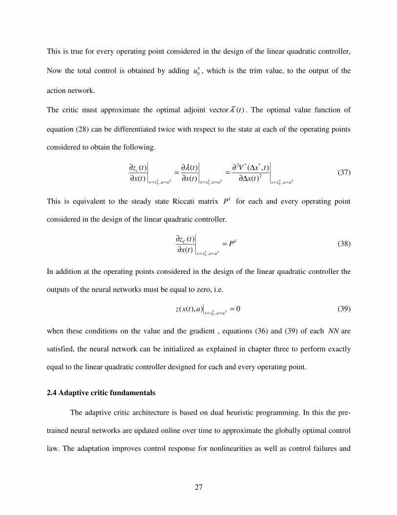
The critic must approximate the optimal adjoint vector )(* tλ . The optimal value function of
equation (28) can be differentiated twice with respect to the state at each of the operating points
considered to obtain the following.
kkkkkkaaxxaaxxaaxx
c
tx
txV
tx
t
tx
tz
======∆∂
∆∂=
∂
∂=
∂
∂
,
2
**2
,, 000
)(
),(
)(
)(
)(
)( λ (37)
This is equivalent to the steady state Riccati matrix kP for each and every operating point
considered in the design of the linear quadratic controller.
k
aaxx
C Ptx
tz
kk
=∂
∂
== ,0
)(
)( (38)
In addition at the operating points considered in the design of the linear quadratic controller the
outputs of the neural networks must be equal to zero, i.e.
0)),((,0
=== kk
aaxxatxz (39)
when these conditions on the value and the gradient , equations (36) and (39) of each NN are
satisfied, the neural network can be initialized as explained in chapter three to perform exactly
equal to the linear quadratic controller designed for each and every operating point.
2.4 Adaptive critic fundamentals
The adaptive critic architecture is based on dual heuristic programming. In this the pre-
trained neural networks are updated online over time to approximate the globally optimal control
law. The adaptation improves control response for nonlinearities as well as control failures and

28
modeling errors. The updating of the action and critic neural network are implemented in
discrete time through an incremental optimization scheme called dual heuristic programming.
Dual heuristic programming is based on the recurrence relation of dynamic programming. The
nonlinear continuous system represented by
),,( tuxfx p=& (40)
is discretized assuming piecewise constant inputs and constant time interval t∆ . The discrete
equivalent of the plant is then given by
),,()1( kpDk tuxftx =+ (41)
In the online phase the same metric that is optimized in the offline training phase is minimized
providing a systematic approach to control design. As with the plant the cost function also needs
to be discretized. The discrete equivalent of the cost of equation (16) is given by
ttuxLJN
k
kDN ∆=∑−
=
1
0
,0 ],,[ , ∞→∆tN (42)
where the discrete form of the Lagrangian in equation (19) is made use of. The integral in the
time domain is converted to the summation in the discrete domain. As in the continuous time
domain, a value function can also be defined for the discrete time domain. The cost of going
from the thk instant, kt , to the final instant of time Nt can be written as
( ) ttuxLtuxLtuxLtxV NDkDkDk ∆+++= −+ ],,[.........],,[],,[),( 11 (43)
But from the discrete state equation, the state )( 1+ktx depends on the current state )( ktx and the
current control signal )( ktu , therefore the cost to go function can be written as
)](),.......(),()[,(],,[),( 1111 −++++∆= NkkkkDk tututxtxVttuxLtxV (44)

29
The objective is now to find a sequence of control such that the cost function or performance
measure is minimized. Therefore the optimal cost for the )( kN − stage policy is found by
minimizing the following functional with respect to the control sequence
{ })(.),........(),([min],[ 1
*
)()........(
**
1
−−
≡ Nkktutu
k tututxVtxVNk
(45)
From the principle of optimality if a policy is optimal over )( kN − stages what ever the initial
state and decision are the remaining decisions must also constitute an optimal policy for the state
obtained from the first decision, i.e. )( 1+ktx , then from equations (44) and (45)
{ }],[],,[min],[ 1
**
)(
*
++∆≡ kkDtu
k txVttuxLtxVk
(46)
This equation is called the recurrence relation of dynamic programming. In normal dynamic
programming the above equation is solved backwards in time starting from the final time to
obtain the optimal control sequence. In forward dynamic programming we use Howard’s form of
recurrence relation given by
],[],,[],[ 1++∆= kkDk txVttuxLtxV (47)
where the cost ],[ 1+ktxV to go from the state )( 1+ktx is a predicted or estimated value obtained
from the critic network. The approximate optimal control at any time, kt , )( ktu is defined as the
one that minimizes the equation (47) for any )( ktx . It has been shown that when the control
)( ktu is calculated to minimize the cost to go function ],[ ktxV based on the above equation the
method converges to the optimal solution over time [19] if the state space is explored completely
and infinitely often.
The control )( ktu that for which the value function is stationary is the optimal control
strategy that minimizes the value function, i.e.

30
0)(
)()(
)(
],,[
)(
],[ 11 =
∂
∂+
∂
∂=
∂
∂ ++
k
k
k
k
kD
k
k
tu
txt
tu
tuxL
tu
txVλ (48)
Recallx
V
∂
∂=λ is the output of the critic network. Since the action network has to generate the
control signal to minimize the cost, equation (48) is used to find )( ktu that is the target for the
adaptation of the action neural network. Note that the critic network is necessary to give
)( 1+ktλ to solve equation (48). In addition a model of the plant is necessary to evaluate the
transition matrix)(
)( 1
k
k
tu
tx
∂
∂ + . The solution of equation (48) gives the optimal control )( ktu . To
obtain the recurrence relation for finding the target value for the critic network training Howard’s
form of the optimal value function is differentiated with respect to the state to obtain
)(
)]([
)(
)()(
)(
)()(
)(
)]([
)(
],,[
)(
],,[
)(
],[)( 1
11
1
k
k
k
kk
k
kk
k
k
k
kD
k
kD
k
kk
tx
txu
tu
txt
tx
txt
tx
txu
tu
tuxL
tx
tuxL
tx
txVt
∂
∂
∂
∂+
∂
∂+
∂
∂
∂
∂+
∂
∂=
∂
∂≡ +
++
+ λλλ (49)
This constitutes the adaptation criteria for the critic network. Equation (49) also requires a model
of the plant in order to determine the transition matrices )(
)( 1
k
k
tx
tx
∂
∂ + and)(
)( 1
k
k
tu
tx
∂
∂ + . When the
adaptation for both the critic and action network are carried out iteratively over time the action
network converges to the optimal control policy.
31
3. ALGEBRAIC TRAINING OF NEURAL NETWORKS
Neural networks are parallel computational paradigms that can approximate nonlinear
mappings between multi dimensional inputs and outputs with relatively small error. Neural
networks are based loosely on biological neural formations and are characterized by their
architecture, the number of neurons and in the order in which they are arranged, and the weights
between their interconnections.
The architecture of the neural network to approximate a given nonlinear mapping between
the input and output is not unique. It is possible to achieve arbitrarily low error between the
desired output and actual output of a network using different kinds of network architecture. In
this chapter, a method is described to determine the architecture and the initial weights of a
neural network by solving a set of linear equations to approximate a nonlinear mapping between
the input and output. This method was developed by Ferrari [16, 20, and 21]. A particular case
that is relevant to control system design used in this thesis is explained in detail.
A set of nonlinear equations to be solved for the neural network adjustable parameters is
obtained by using the training set of inputs and outputs and the gradient of the output with
respect to either all or some of the inputs. The function to be approximated is usually not known
analytically, but the set of inputs, ky , corresponding outputs, ku and gradients k
C are available in
the form{ }Kk
kkkCuy ,....1,, = . The neural network approximates the functional relationship
)( kk ygu = between the input and output. The neural network can improve generalization if the
gradient information kC is also used [16]; hence they are also incorporated into the training set.
The output of a neural network of the form shown in Figure 7 is given by the nonlinear
equation
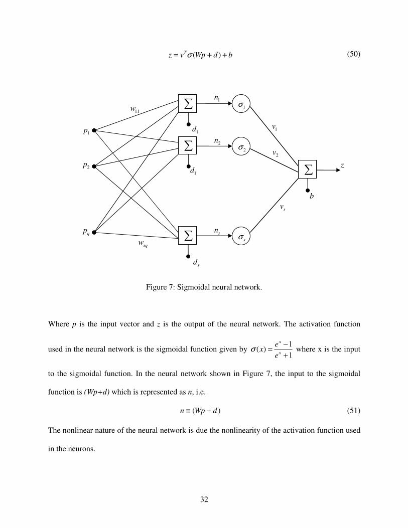
32
bdWpvz T ++= )(σ (50)
Figure 7: Sigmoidal neural network.
Where p is the input vector and z is the output of the neural network. The activation function
used in the neural network is the sigmoidal function given by 1
1)(
+
−=
x
x
e
exσ where x is the input
to the sigmoidal function. In the neural network shown in Figure 7, the input to the sigmoidal
function is (Wp+d) which is represented as n, i.e.
)( dWpn +≡ (51)
The nonlinear nature of the neural network is due the nonlinearity of the activation function used
in the neurons.
sd
sv
2v
1v
z
b
1d
1d
2n
sn
1n
sqw
11w
qp
2p
1p
∑
∑
∑
1σ
2σ
sσ
∑

33
The input weights W, the output weights v, together with the input bias d and b constitute the
parameters of the neural network that can be adjusted to approximate the input output
relationship. To match a given input output set the neural network output must satisfy the
nonlinear equation
bdWyvu kTk ++= )(σ , Kk ,....2,1= (52)
which can be represented by a vector equation for all the K training pairs.
bSvu +=
b is an s-dimensional vector, equal to the number of neurons in the neural network, composed of
the scalar output bias, b. S is a matrix of sigmoidal functions evaluated at input to node values,
k
in , each representing the magnitude of the input-to-node variable.
≡
)()()(
)()()(
)()()(
111
22
2
2
1
11
2
1
1
KKK
s
s
nnn
nnn
nnn
S
σσσ
σσσ
σσσ
M
L
MM
L
L
(53)
The known gradient, kc , corresponds to the partial derivatives of the neural network’s
output with respect to its inputs evaluated at the training pair k. Exact matching of the gradient
set is obtained if the neural network satisfies the gradient equation[16].
{ },)()1,( kTk nveWc σ ′⊗→•= Kk ,....1= (54)
Where the symbol “ ⊗ ” denotes element-wise vector multiplication, and )1,( eW →• represents
the first e columns of the input weight matrix for which the gradients are known. Equation (54)
can be rewritten as
Tkk eWBc )]1,([ →•= , Kk ,....1= (55)
With the matrix

34
])(.......)()([ 2211
k
ss
kkknvnvnvB σσσ ′′′≡ , Kk ,....1= (56)
3.1 Exact gradient based solution
As stated earlier for the neural network based nonlinear controller used in this thesis to
perform as well as the gain matrices they replace, the gradient of the function defined by the
neural network should equal the gains at the corresponding operating points. At the operating
point the output of the neural networks is zero since the perturbed input states )(tx is zero.
Therefore the training pairs are a set of points of the form{ }Kk
kkcy ..2,1,0, = . The input to the
network can be partitioned at the design points into Kk
TkkkT
axy....2,1
]|0[=
== as both the states
of the system and scheduling variables are fed as inputs to the neural network. Therefore the
training set can be written as{ }Kk
kTkca
T
....2,1,0,]|0[ = . Now the output of the neural network can be
written using the nonlinear equation (50) as
bdaWWvTk
ax
TT
++= )]|0][|([0 σ , Kk ...2,1= (57)
Now we see that the output equation does not depend on the weights associated with the
perturbed states )(tx , and the equation reduces to
bdaWvTk
a
TT
++= )]][([0 σ , Kk ...2,1= (58)
Now the gradient equation (54) can be written as
}]][([{ daWvWcTk
a
T
x
kT
+′⊗= σ , Kk ...2,1= (59)
Since the gradient of the function is known only for the state and not for the scheduling variables
only the weights xW , associated with the states are considered. From equation (51), the input to
node values n can be represented as

35
daWnk
a
k
i +≡ , Kk ...2,1= , si ......2,1= (60)
Now if we know all the inputs to the hidden nodes the output equation becomes linear in the
output weights and is given by
Svb −= (61)
If we choose the number of nodes in the hidden layer equal to the number of training pairs, the
matrix S is square, the above equation can then be solved for a unique v for an arbitrary b if S is
also non singular. In the thesis the vector b is generated using MATLAB function rand.
Now the gradient equation (59) can also be treated as linear and be represented as
xXwC = (62)
The unknowns in the above equation consist of the input weights xw . The matrix wx consists of
the weight matrix Wx rearranged into a vector form, which consists of column wise
reorganization of the matrix elements into a vector [16]. The vector C is the known gradients in
the training set,
TKTT
ccC ]|....|[ 1≡ (63)
and X denotes a sparse matrix composed of block diagonal submatrices each of size ese ×
−
−
−
−
−
−
−
−
−
−
≡
p
p
p
B
B
B
B
B
B
X
:
0
0
0
:
0
0
0
:
0
0
0
:
0
0
:
0
0000
:::::
0000
0000
1
1
1
MMMMM (64)
36
Every block Bk is known when v and all input-to-node values are known from equation (56) and
kn depends only on aW , furthermore when the number of hidden nodes is equal to the number of
training pairs, X is a square matrix and can be solved to give a unique value for wx provided X is
also non singular.
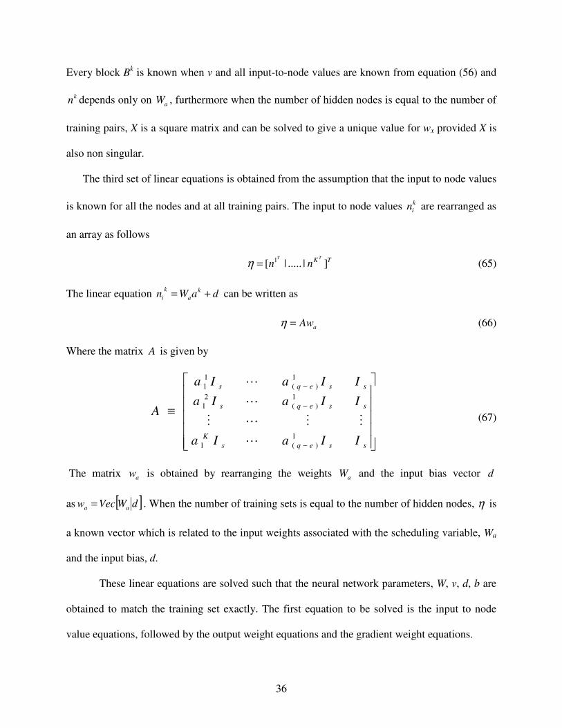
The third set of linear equations is obtained from the assumption that the input to node values
is known for all the nodes and at all training pairs. The input to node values k
in are rearranged as
an array as follows
TK TT
nn ]|.....|[ 1=η (65)
The linear equation daWnk
a
k
i += can be written as
aAw=η (66)
Where the matrix A is given by
≡
−
−
−
sseqs
K
sseqs
sseqs
IIaIa
IIaIa
IIaIa
A
1
)(1
1
)(
2
1
1
)(
1
1
L
MMLM
L
L
(67)
The matrix aw is obtained by rearranging the weights aW and the input bias vector d
as [ ]dWVecw aa = . When the number of training sets is equal to the number of hidden nodes, η is
a known vector which is related to the input weights associated with the scheduling variable, Wa
and the input bias, d.
These linear equations are solved such that the neural network parameters, W, v, d, b are
obtained to match the training set exactly. The first equation to be solved is the input to node
value equations, followed by the output weight equations and the gradient weight equations.

37
Since the number of nodes, s, is equal to the number of training pairs, p, A and C are
determined from the equations (67) and (66) respectively. The vector η is determined so that the
matrix S is well conditioned. One strategy for producing a well conditioned S is to generate the
vector η as follows
=0
,k
ik
i
rn
ki
ki
=
≠ (68)
where k
ir is chosen from a normal distribution with mean zero and variance one. Now an
estimate of aw can be obtained by solving the following equation
ηPI
a Aw =ˆ (69)
aw is the best approximation to the solution. When this value for aw is substituted into the
equation
awA ˆˆ =η (70)
we get the vector η and from this T
snnn )]().......([][ 1 σσσ ≡ is obtained. Now S can be computed
from the vector ηη ˆf= , where f is a factor such that each sigmoid is centered for a given input
ky and is close to saturation for any other known input. The weight matrix aw is now obtained
using the relation
aa wfw ˆ= (71)
Once S is known the output weight matrix v can be obtained. With the solution of v andη , the
matrix X can be formed from which the weight xw can be obtained.
Thus the neural network can be initialized guaranteeing that the neural networks meet the
performance specification of the linear gain matrices that they replace. This concludes the
initialization phase of the adaptive critic design.

38
4. LINEAR CONTROL DESIGN
The neural network controller is based on a linear controller which is designed using
linear control theory for a set of models linearized about equilibrium points. In this chapter the
design process of a linear controller for the longitudinal model of an aircraft is explained. The
linear controller establishes the performance requirements to be met by the system. As explained
in chapter three the linear controllers are used to determine the architecture and initial weights of
the neural network. When the neural networks are initialized as outlined in chapter three the
neural network controller performs as well as the linear controllers that they replace at the design
points .
Simulations carried out with the longitudinal model show that the initialized neural
network controller performs as well as the linear controller designed at the operating points. The
neural network based controller is also able to perform as well as a gain scheduled linear
controller at interpolation points between the design points considered in the operating envelope
of the aircraft. The online training phase improves the controller’s performance in the presence
of nonlinearities as well as for unanticipated control failures and parameter variations between
the actual model and the assumed model. The online training phase of the controller is described
in chapter five.
The operating envelope of the aircraft is as shown in Figure 8. It can be divided into the
set of operating points, called OP considered in the initialization phase. The points that are
within the area enclosed by the design points considered in the initialization phase is called the
interpolating region abbreviated as IR. The region which is outside the area enclosed by the
design points considered in the initialization phase is called the extrapolating region ER.

39
120 140 160 180 200 220 240 260 2800
0.2
0.4
0.6
0.8
1
1.2
1.4
1.6
1.8
2x 10
4
Velocity [ft/s]
Altitude [ft]
ERIR
OR
Figure 8: Operating envelope
The longitudinal model of the aircraft is available in terms of the stability derivatives. Since
only the longitudinal model of the aircraft is available the controller is designed to follow
longitudinal pilot commands for the flight path angle γ and forward velocity V. The controller is
designed using the state vector TqVx ][ θγ= comprising the airspeed, flight path angle,
the pitch rate and the pitch angle. The scheduling vector ][ hVa = is comprised of the airspeed
and altitude respectively. The control inputs to the aircraft to control longitudinal flight are the
throttle and the elevator, therefore the control vector u is given byT
eTu ][ δδ= . The pilot
command is represented by the vectorT
CCC Vy ][ γ= .
40
4.1 Flight envelope
The operating envelope of the general aviation aircraft needs to be determined based on
the stall speed of the aircraft, the thrust available and the maximum allowable dynamic pressure
to prevent structural damage. Once the operating envelope of the aircraft is available the
equilibrium points can be chosen on the envelope boundaries and inside the envelope to design
the linear controllers. This section explains the process in determining the envelope of the
general aviation aircraft used in this thesis.
The range of velocities at which an aircraft can fly is limited on the lower end by the stall
speed and at the higher end by the maximum power available. The upper end of the altitude to
which an aircraft can fly is limited by the power available at a particular altitude.
The stall speed of an aircraft is defined as the minimum airspeed at which one can maintain
straight level flight. The stalling speed of an aircraft depends on the maximum lift coefficient of
the aircraft max,LC . The stall velocity of the aircraft is given by
max,
2
L
StallSC
WV
∞
=ρ
(72)
where W is the weight of the aircraft, S is the wing reference area, ∞ρ is the density of ambient
air and max,LC is the maximum lift coefficient of the aircraft. The stall velocity changes with
altitude as the density of air decreases with altitude. The stall velocity therefore increases as the
aircraft flies at higher altitude. Since the stall velocity is the minimum velocity at which the
aircraft can maintain steady level flight it forms the low speed end curve in the flight envelope.
At the high end the maximum velocity at which an aircraft can fly is determined by the
maximum power available. As an aircraft flies at higher velocities, the drag of the aircraft
increases and to balance this in steady level flight an equivalent amount of thrust is necessary.

41
The thrust available for a given engine depends on the engine itself as well as the altitude at
which the aircraft is flying. In the present context the data for actual engine thrust variation with
altitude was not available directly. In order to compute the max velocity at which the aircraft
could fly at a given altitude the rate of climb performance of the general aviation aircraft at
various airspeeds, was obtained from the pilot’s operating handbook.
The rate of climb of an aircraft at a given velocity ∞V is given by
Rate of climb =W
DVVTA ∞∞ − (73)
Where AT the maximum available thrust of the aircraft, D is the total drag and ∞V is the airspeed
or velocity of the aircraft. The numerator in the rate of climb equation is the difference between
the power available, ∞= VTP AA , and the power required, ∞= VTP RR , to fly level at a given
velocity. We can calculate the power required to fly at the velocity for which the rate of climb of
the aircraft is known, from this we can calculate the total power available at a given altitude.
Once we have the total available power at a given altitude we can calculate the maximum
velocity at which the aircraft can fly at that particular altitude solving the equation.
max
24
max
2
20 VPVP
SeAR
WV
SCAR
D==+ ∞ρπ
ρ (74)
and taking the maximum value of the real roots.
In the design of the nonlinear controller presented in this thesis, the lower end of the
design region IR is based not on the stall speed at a given altitude, but on the airspeed for level
flight of the aircraft at minimum thrust. The reason for this is to avoid flying the aircraft on the
backside of the power curve where a decrease in velocity ∞V requires an increase in power. The
airspeed at minimum thrust for a reciprocating engine and propeller configuration is given by
[26].

42
0
2min
D
TC
eAR
S
WV
π
ρ= (75)
where W is the weight of the aircraft, S the wing reference area, ρ is the density of air, e is the
oswalds efficiency factor, AR is the aspect ratio of the wing, 0DC is the drag at zero lift.
Once the envelope bounded by the airspeed at minimum thrust on the lower end and the
maximum velocity at the higher end at different altitudes is known, we can now choose the
operating (design) points within and on the boundary of the envelope. A total of thirty six
operating points were chosen as shown in Figure 9. The small perturbation model about these
steady state operating points are obtained and used for designing the linear controllers.
160 180 200 220 240 260 2800
0.2
0.4
0.6
0.8
1
1.2
1.4
1.6
1.8
2x 10
4
Velocity [ft/s]
Alti
tud
e [
ft]
Figure 9: Flight envelope

43
4.2 Linear controller design
At each of the thirty six operating points considered in the flight envelope of the general
aviation aircraft, linear controllers are designed such that they meet required system
specification. These controllers provide the performance baseline for the nonlinear neural
network controller. The three longitudinal equation of the aircraft are linearized at different
operating points based on the scheduling vector a. A small perturbation model of the nonlinear
equation is obtained at each and every operating point of the form
)()( tuGtxFx ∆+∆=∆& (76)
The matrices F and G are linear and time invariant. As this process is carried at each and every
operating point it results in a set of thirty six F and G matrices indexed by 36.....2,1=k . Linear
control theory is used to design controllers using the F and G matrices at each operating point.
The perturbation model for the longitudinal model is a fourth order linear differential
equation of the form given below
)()( tuGtxFx LL ∆+∆=∆& (77)
where the longitudinal state matrix is TqVx ][ θγ= and the control matrix is
T
ETu ][ δδ= . The linear controllers designed for the set of linear models are used to initialize
the feedback, command-integral, which are combined to form the action network, and critic
neural networks.
The linear controllers to be designed are based on a Proportional-Integral (PI) linear
control structure. A PI controller shown in Figure 10 can be designed to modify the stability of
the system and the transient response to meet performance specifications. The PI controller
achieves this using the feedback gain matrix BC , the system response is guaranteed to be a type-1

44
response [23] to command inputs through the proportional gain matrix FC , and the command
integral gain matrix IC . The linearized output equations about the nominal conditions is given by
)()()( tuHtxHty uxs ∆+∆=∆ (78)
The objectives of the control system are evaluated based on the performance measure of the form
ττ duxLJ
f
f
t
at
],~,[2
1lim
0
∫∞>−= (79)
= τττττττ duRuuMxxQx a
T
aaaa
t
T
at
f
f
)](~)(~)(~)(2)()([2
1lim
0
++∫∞>− (80)
which is minimized with respect to u~ . ax represents an augmented state that is given by
TTT
a xx ]~[ ξ≡ where
cc xxxxxxx −=−−−≡ )()(~00 (81)
is the error between the actual state x and the commanded state cx and 0x is the equilibrium
state. ξ is the time integral of the output error.
Figure 10: PI controller
FC
∫
BC
Linear
Plant
uH xH
IC
+
+
+ +
-
-
-
)(~ ty
)(tys∆
)(tu∆
)(tx∆ )(tyc

45
The output error and the minimizing control are also defined as the perturbation from the set
point [ ]CCV γ commanded by the pilot, i.e. Cs yyy −≡~ and cuuu −≡~ . The optimal control
deviation to minimize the performance measure can be shown to be given by [23].
[ ]TttxI
CB
Cta
xa
Ctu )()(~][)()(~ ξ−=−= (82)
The control gain matrix aC , is partitioned into the two matrices BC and IC
)()(~)(~ tCtxCtu IB ξ−−= (83)
The proportional gain matrix FC is obtained from the feedback gain matrix and set point
matrices[16].
1222 BCBC BF += (84)
For the linearized system, the set point is defined by letting the state-rate perturbation x&∆ equal
to zero. This gives the steady state flight condition
∆
∆
=
c
c
uxC u
x
HH
GF
y
0 (85)
The set point state and control perturbations are obtained from the command perturbation as
given
∆
∆=
∆
≡
∆
=
∆
∆−
C
C
CCuxc
c
yB
yB
yBB
BB
yHH
GF
u
x
22
12
2221
1211
100
(86)
The Riccati matrix, aP , needed to train the critic network is obtained by solving the matrix
Riccati equation given in equation (31) constructed in terms of the augmented state and control
deviation. The weighting matrices in the performance measure are formulated using implicit
model following as explained in the next section.

46
4.2 Implicit model following
In formulating the weighting matrices RMQ ,, in equation (80) in the performance
measure we use implicit model following to induce the closed loop system to follow the response
of an ideal model that meets performance specifications. The ideal model which the system has
to follow is a linear model of the same order as the linearized longitudinal model of the aircraft.
The selection of an ideal model for longitudinal control of an aircraft is based on handling
quality requirements that meet either civilian or military specifications for different aircraft types
and phases of flight.
The general aviation aircraft for which the nonlinear neural controller is designed is
classified as a class I aircraft. The longitudinal flying qualities of the aircraft are specified by
imposing boundaries on the damping ratio of the two modes, phugoid and short period, which
characterize the longitudinal response of the aircraft. The boundaries for the damping ratio vary
based on the flight phase. Accurate following of the pilot input commands are necessary during
the terminal flight phase conditions like takeoff and landing. The boundaries of the damping
ratio of the short period and phugoid mode for the terminal flight phase for a class I aircraft are
given in Table 1 [24]
Longitudinal flying qualities
Phugoid mode
04.0>pζ
Short-period mode
30.135.0 ≤≤ spζ
Table 1: Flying qualities for class I aircraft in terminal phase flight

47
The ideal model of the longitudinal motion of the aircraft using the stability derivatives
with the state perturbation [ ]TqVx αγ ∆∆∆∆=∆ is given by [25]
−−−−
−
=
00000
00000
0
/)/1(sin)/(/
0
//sin)/(/
cos
VLVLVgVL
MMM
VLVLVgVL
TDTDgTD
F
qv
qv
qv
qv
m
α
α
α
α
γ
γ
γ
(87)
The above matrix mF for the ideal aircraft which is in approximate block diagonal form and can
be partitioned into the phugoid parameters and short period parameters.
The phugoid damping ratio and the short period can be determined by the following
formulae
)/( 0VgLvnp ≈ω (88)
npvp TD ως 2/−≈ (89)
)/)/1(( 00 VLMVLM qqnsp ααω −−−≈ (90)
nspqsp MVL ως α 2/)/( 0 −≈ (91)
The matrix F for the ideal model can be computed based on the flying qualities to be met by the
actual aircraft. As there are more parameters than the number of equations, certain values can be
assumed to be equal to the actual aircraft. In this thesis we equated the 0/VLq , qTD , vM , αM ,
0/VLα , αTD and 0/VLv to be equal to the median value of the thirty six linearized models
obtained at each operating point. The next step is to solve the equations obtaining the desired
values of the natural frequency and damping ratio.

48
The desired value of the damping ratio for the phugoid mode and the short period mode
of the ideal model were selected to be 1.0≈pς and 1≈spς . These values were then used to
determine the parameters vTD and qM using equations (89) and (91).
The ideal model obtained needs to be transformed into the same state vector as the
system to be controlled. In this thesis we are designing for pure longitudinal motion for which
the relationship between the flight path angleγ , the angle of attack α and the pitch angle θ is
given by
αγθ += (92)
Now the transformation matrix T is given by
=
1010
0100
0010
0001
T (93)
The transformation from the state [ ]TqVx αγ ∆∆∆∆=∆ to [ ]Tm qVx θγ ∆∆∆∆=∆ is
given by
∆
∆
∆
∆
−−−−
−
=
∆
∆
∆
∆−
α
γ
γ
γ
γ
θ
γ
α
α
α
α
q
V
VLVLVgVL
MMM
VLVLVgVL
TDTDgTD
q
V
qv
qv
qv
qv
1
00000
00000
0
1010
0100
0010
0001
/)/1(sin)/(/
0
//sin)/(/
cos
1010
0100
0010
0001
(94)
[ ]
∆
∆
∆
∆
=
∆
∆
∆
∆
α
γ
θ
γ
q
V
Fq
V
m (95)
Now the state equation of the ideal model is given as

49
)(txFx mmm ∆=∆& (96)
In implicit model following the state rate of the actual system should be the same as that of the
ideal model. Since we need the actual system states to follow the ideal model states, the
performance measure or cost function to be minimized can be given by the following
{ } τττττ dxxQxxJ
f
f
t
t
mm
T
mt ∫ ∆−∆∆−∆=
∞>−0
))()(())()((2
1lim &&&& (97)
This is equal to
[ ] ττττττ duRuuMxxQxJ
ft
TTT
∫ ∆∆+∆∆+∆∆=0
)()()(2)()(2
1 (98)
when the weighting matricesQ , M , R are given by equations (99),(100) and (101) respectively
)()( mm
T
m FFQFFQ −−= (99)
GQFFM m
T
m )( −= (100)
0RGQGR m
T += (101)
The matrices G and F are the control and system matrix from the perturbation model equation
76 is obtained at each operating point. The matrix 0R is a constant matrix which represents the
separate cost of control. The actual system follows the ideal model when the following condition
is satisfied [23].
0))(( =−− mn
PIFFIGG (102)
Since the actual system model F is not exactly equal to the ideal model mF perfect model
following cannot be achieved. The weighting matrices mQ and 0R can now be chosen such that
the actual response that follows the ideal model response for the pilot input commands of flight
path angle and velocity with reasonable amount of control input.

50
In order to achieve a type one response, the integral of the error between the commanded
velocity and flight path angle needs to be considered in the cost function. We need to augment
the states with the error integral ξ leading to the cost function given by
[ ] ττττττ duRuuMxxQxJ
ft
a
T
a
T
aaa
T
a∫ ∆∆+∆∆+∆∆=0
)()()(2)()(2
1 (103)
where T
a xx ][ ξ∆=∆ is the state augmented by the error integral and the matrices aQ and aM
are given by
=
ξQ
QQa 0
0 (104)
=
0
MM a (105)
RRa = (106)
The output equation for the linearized model is given by
)(]0[)(0010
0001)( tutxty a ∆+∆
= (107)
Now the PI gains for all the thirty six models are calculated by solving the Riccati equations of
the form given in equation (31) using the weighting matrices aQ , aM and aR resulting in thirty
six control gain matrices { } 36......1C and Riccati matrices { } 36....2,1
P . The gain matrices { } 36......1C are
used to obtain the set of feedback matrices{ } 36...2,1
BC , the set of integral matrices { } 36...2,1
1C and the
forward gain matrices{ } 36....2,1
FC of Figure 10 using equations (83) and (84).

51
4.3 Neural network based controller
The next step after the design of the linear controllers is to replace the gain matrices with
neural networks. Each of the feedback matrices, the integral matrices are replaced with a neural
network and are initialized such that they meet performance specifications of the linear controller
they replace, These two networks are combined to form the action network. The neural network
based controller is as shown in Figure 11.
Figure 11: Neural network based PI controller
As seen from Figure 11, the input output structure is unchanged from the linear controller. The
output )(ty and the set point ),( cc ux are computed for the nonlinear system. The scheduling
variable generator produces the scheduling variable inputs to the neural networks. The command
state generator uses the kinematic equations to generate the other elements of the state such that
they are compatible with the pilot input command of velocity and flight path angle. The two gain
)(tyc
FC
∫
BNN
Nonlinear
Plant
uH xH
INN
+
+
+ +
-
+
+
)(~ ty
)(tys
)(tu )(tx
SVG
CSG
)(ta
)(txc
)(tuc
)(tuI∆
)(tuB∆ )(~ tx +
-

52
matrices, feedback gain matrix BC , and the integral matrix IC are replaced by the neural networks
designated as BNN and INN respectively. The forward matrix FC , which is used to calculate the
commanded state cx and the commanded Tδ and Eδ ,can also be replaced by an equivalent neural
network. But in this thesis the forward gain matrix is retained from the linear design.
The inputs to all the neural networks consist of the scheduling variables
TtHtVa )]()([= . In addition the neural networks BNN and INN are the state deviation )(~ tx and
the command-error integral )(tξ respectively. The total control signal is the addition of the
output from the forward gain matrix, the output of the feedback neural network and the output of
the integral neural network, i.e.
)()()()( tutututu IBc ∆+∆+= (108)
The next step in the design of the neural network based nonlinear controller is to
determine the architecture and the initial weights of the neural network. The methodology
presented in chapter three is used now to determine the initial weights and architecture of the
feedback neural network and the integral neural network.
At the operating points considered, the output of the feedback neural network must be
zero. This is true because at the operating point the state )(tx approaches the commanded state
)(txc and )(~ tx tends to zero. Therefore
0)](,0[)](),(~[ == KBKB taztatxz (109)
The control deviation )(~ tu is the difference between the commanded input )(tuc generated by
the forward matrix and the sum of the control inputs generated by the feedback neural network
and the integral neural network, i.e.
)()()()()(~ tztztututu IBIB +=∆+∆= (110)

53
Differentiating the above equation with the state deviation at the operating point we get
( )K
B
KK
B Ctx
u
tx
tz−=
∂
∂=
∂
∂
)(~
~
)(~)(
(111)
Similarly the output of the integral neural network is zero when the command error integrals are
zero, i.e.
0)](,0[)](),([ == KIKI taztatz ξ (112)
and the derivative of the integral neural network with respect to the command error integral is
given by
( )K
I
KK
I Ct
u
t
tz−=
∂
∂=
∂
∂
)(
~
)(
)(
ξξ (113)
Now the training set for the feedback neural network is a set of thirty six input output pairs of the
form { }K
B
TKCa
T
,0,]0[ for the thirty six operating points considered. Similarly the training set
for the integral neural network is of the form{ }K
I
TKCa
T
,0,]0[ . Initially the neural networks for
each of the control signal, i.e. Tδ and Eδ , is trained separately by only considering the
corresponding rows of the gradient matrices BC and IC , in the next chapter these are combined
and used to generate the total control deviation signals.
Now the gradient based procedure explained in chapter three is used to initialize both the
feedback and the integral neural network. Both the neural networks are composed of single
hidden layer sigmoidal neural networks with the number of neurons equal to the number of the
training pairs. One important feature of the neural network is that the direct contribution of the
scheduling variables to the output of the neural network is subtracted using a mirror image of the
initialized network. This is done to eliminate any bias the scheduling variables might produce
away from the nominal condition. This is done to prevent the neural network from adapting for a

54
change in the scheduling variables of V and h . The final architecture for the initialized feedback
neural network for one of the control signals is shown in Figure 12 and for the integral neural
network is shown in Figure 13.
Figure 12: Initialized feedback neural network architecture
+
-
σ
σ
σ
σ
V~
γ~
q~
θ~
V
V
H
H
BTδ∆

55
Figure 13: Initialized integral neural network architecture
4.4 Response of initialized neural network
The initialized neural network are now tested and evaluated with respect to the linear
controller that they replace. The neural network controller is tested on the longitudinal model of
the aircraft. The neural network controller response is then compared to the linear controller
response designed for the operating point considered. In order to test the generalization
properties of the neural network, the response of the neural network controller is also evaluated
τdV
t
∫0
~
+
-
σ
σ
σ
σ
τγ d
t
∫0
~
V
V
H
H
ITδ∆

56
at a point other than the operating point called the interpolation point. In order to compare the
performance of the neural network controller a linear controller is designed for the interpolation
point considered but not used in initializing the neural network.
Case 1: Response at a design point
The neural network controller response is evaluated at the design
point )5000,74.211(),( 00 ≡hV . The response of the controller to a two degree step command in
the flight path angle and three feet per second step increase in the velocity is considered. Figure
14 shows the variation of the flight path angle and velocity.
0 1 2 3 4 5 6 7 8 9 10211.5
212
212.5
213
213.5
214
214.5
215
215.5
216
Velo
city - m
/s
0 1 2 3 4 5 6 7 8 9 10-1
-0.5
0
0.5
1
1.5
2
2.5
3
3.5
Time-s
Clim
b a
ng
le -
de
g
Linear Controller
NN Controller
Linear Controller
NN Controller
Figure 14: Response at a design point
Case 2: Response at an interpolation point
The neural network controller response is evaluated at the Interpolation point
)4000,209(),( 00 ≡hV . The response of the controller to a two degree step command in the flight

57
path angle and three feet per second step increase in the velocity is considered. Figure 15 shows
the variation of the flight path angle and velocity.
0 1 2 3 4 5 6 7 8 9 10208.5
209
209.5
210
210.5
211
211.5
212
212.5
213
Velo
city -
m/s
0 1 2 3 4 5 6 7 8 9 10-1
-0.5
0
0.5
1
1.5
2
2.5
3
3.5
Time-s
Clim
b a
ngle
- d
eg
Linear Controller
NN Controller
Linear Controller
NN Controller
Figure 15: Response at an interpolation point
4.5 Critic neural network
The critic neural network, CNN , is used to evaluate the performance of the action network
online with the dual heuristic programming adaptive critic architecture. The critic evaluates the
performance by approximating the derivative of the cost to go or value function. The critic
network is also initialized as the other two neural networks, the feedback neural network and the
integral neural network.
The critic neural network is not used in the testing of the initialized controller as the
weights of the feedback and the integral neural network are not adapted. In the online phase the
weights of the action network, which is obtained by combining the feedback and integral neural

58
network, is adapted to improve performance in the presence of nonlinearities as well as control
failures. The critic neural network optimizes the same cost function that is optimized in the pre-
training phase as described in section 2.4. The critic network approximates the derivative of the
value function given by
)(
),()]([
tx
txVtx
a
aa
∂
∂≡λ (114)
Thus the output of the critic neural network is given by
]),([)( atxzt aCa =λ (115)
For the set of operating points considered in the linear controller design, the state deviation
)(~ tx and the command error integral )(tξ are equal to zero. Therefore the output of the critic
neural control at the operating point is zero, i.e.
( ) ( ) 0],0[)](),([ ==K
C
K
aC aztatxz (116)
The gradient of the critic neural network with respect to the augmented state is given by
)(
)(
)(
)(
tx
t
tx
tz
a
a
a
C
∂
∂=
∂
∂ λ (117)
At the operating points considered the derivative of the value function with respect to the
augmented state is given by
k
a
T
a
k
a
a Ptxtx
txV)(
)(
),(=
∂
∂ (118)
Therefore the gradient of the critic neural network must satisfy the condition
k
a
k
a
a
k
a
C Ptx
t
tx
tz=
∂
∂=
∂
∂
)(
)(
)(
)( λ (119)

59
Now a training set of the form { }K
a
TKPa
T
,0,]0[ similar to the feedback and integral neural
network training sets is available. The initialization can be now done based on the algebraic
training explained in chapter three. As before six different neural networks are initialized
separately and combined as explained in chapter five. The initialized critic neural network for
one of the six outputs is as shown in Figure 16.
Figure 16: Initialized critic neural network.
+
-
σ
σ
σ
σ
V~
γ~
q~
θ~
τdV
t
∫0
~
τγ d
t
∫0
~
V
V
H
H
V
V~
∂
∂

60
5. ADAPTIVE CRITIC FLIGHT CONTROL
In this chapter the neural networks initialized in chapter four are adapted online based on
the dual heuristic adaptive critic design to account for nonlinearities not considered in the linear
control design. The neural network controller also adapts to control failures as well as parameter
variations online. The dual heuristic adaptive critic design is based on the approximate dynamic
programming introduced in chapter one. Approximate dynamic programming iterates only on
one value of the state and uses these results during the next time step. This eliminates the need
for expanding and storing the state vector over time. It has been shown that when the iterative
successive approximation concept is used with a parametric structure to predict the cost, the
solution converges over time to the optimal trajectory.
Neural networks are the parametric structure of choice as they have properties which lend
themselves to approximate functions of multi input multi output space. In dual heuristic dynamic
programming the neural networks are used to approximate the gradient of the value function with
respect to the state. It has been observed that using the gradient of the cost accelerates the
convergence to the optimal trajectory and it alleviates the need for persistence of excitation of
the network. In dual heuristic dynamic programming the control law, approximated by the action
network, and the gradient of the value function, approximated by the critic network, are adapted
based on the recurrence relation of dynamic programming as detailed in section 2.4.
The use of neural networks as function approximators allows for both incremental learning as
well as learning in batch mode. As explained in chapter four, the neural networks are intialized in
batch mode in the pre training phase using the gains obtained from the linear controller design at
the operating point. In the online phase the neural networks learn online to improve system
performance incrementally overtime in the presence of nonlinearities as well as control failures

61
and modeling errors. One important aspect of the online training is that it preserves the mapping
of input and output obtained in the initialization phase. The online training algorithm is based on
the dual heuristic programming explained in the next section.
5.1 Dual heuristic adaptive critic
The online logic is implemented in discrete time with the action and critic network
updating and control action occurring for every time interval t∆ . In the online phase the same
metric or cost optimized in the design of the linear controllers is used. This establishes the input
output structure of the neural network to be the same as that of the neural networks initialized in
the pre training phase. The utility function in discrete time is given by
)](~)(~)(~)(2)()([2
1)](~),([ kak
T
kakakaak
T
akkaSD tuRtutuMtxtxQtxtutxL ++= (120)
where ax is the augmented state [ ]Tx ξ~ and u~ is the control deviation from the nominal control
input. The utility function can also be seen as the cost associated with going from the current
state )( ka tx to the next state )1( +ka tx which depends on the input control deviation )(~ktu . The
weighting matrices aQ , aM and aR are the same as used in the linear controller design in the pre
training phase.
5.2 Action and critic networks
In the pre training phase the neural networks for the integral gain and the feedback gain
were trained independently of each other, also the neural networks for the two control inputs
[ ]TET δδ were initialized separately. In the online training phase the neural networks are
combined to obtain a single action network which encompasses all the four individual networks
initialized in the pre training phase.

62
The networks obtained in the pre training phase must be combined to a single network
and still meet the performance specifications, i.e. the action network obtained by combining the
networks should be equivalent to the individual neural networks. The new network is different
from the neural networks in the pre training phase in that they have a vector output as shown in
Figure 17 as opposed to a scalar output.
Figure 17: Vector output neural network.
The vector output sigmoidal architecture is used for both the action and critic network in the
online training phase. The output of the vector output sigmoidal neural network is given by
bdWpVz ++= )(σ (121)
sd
12v
11v
2z
2b
1d
1d
2n
sn
1n
sqw
11w
qp
2p
1p
∑
∑
∑
1σ
2σ
sσ
∑
1z
1b
∑
rz
rb
∑
1rv
sv1
rsv
sv2

63
The vector-output neural network notation is equivalent to that of the scalar output neural
network. The only difference being that the output weights are now a matrix }{ livV = , where
liv is the weight for the connection between the thi node and th
l output of the network.
To obtain the vector output sigmoidal neural network for the action network, the four
initialized neural network are combined. First the neural networks for the different control inputs
are combined, and then the resulting neural networks for the feedback neural network and
integral neural network are combined. For combining the two networks for the feedback neural
network, it is observed that the inputs to the two neural networks are the same but the outputs are
different, one for the throttle and the other for the elevator. It can be shown that the two neural
networks can be combined such that they retain all the characteristics of the individual networks.
The new neural network has the form as shown in Figure 17. The number of nodes in the
combined neural network is equal to the sum of the number of nodes in the individual neural
network. The input weights, the output weights and the biases are given by
=
E
T
B
B
B W
WW
δ
δ
(122)
=
E
T
B
B
B V
VV
δ
δ
0
0 (123)
[ ]TT
B
T
BB ETddd
δδ= (124)
and
[ ]TT
B
T
BB ETbbb
δδ= (125)
where TBW
δ is the input weight matrix of the feedback network for throttle.
EBWδ
is the input
weight matrix of feedback network for elevator. TBV
δand
EBVδ
are the output weight vectors of the

64
feedback network for throttle and elevator respectively. The input biases of the feedback network
for throttle and elevator are TBd
δand
EBdδ
. the output biases of the feedback network for throttle
and elevator are TBb
δand
EBbδ
. The combined feedback neural network performs equivalent to
the uncoupled feedback networks that it replaces.
Similarly for the integral neural network the two neural networks can be joined together
to obtain a single neural network of the form given above. The combined neural networks
weights are given by
=
E
T
I
I
I W
WW
δ
δ
(126)
=
E
T
I
I
I V
VV
δ
δ
0
0 (127)
[ ]TT
I
T
II ETddd
δδ= (128)
and
[ ]TT
I
T
II ETbbb
δδ= (129)
where TIW
δ is the input weight matrix of the Integral network for throttle.
EIWδ
is the input weight
matrix of feedback network for elevator. The output weight vectors of the feedback network for
throttle and elevator respectively are TIV
δand
EIVδ
. The input biases of the feedback network for
throttle and elevator are TId
δand
EIdδ
. The output biases of the feedback network for throttle and
elevator are TIb
δ
andEIb
δ. The combined integral neural network performs equivalent to the uncoupled integral
networks that it replaces.

65
The next step is to combine the integral neural network and the feedback neural networks
into a single neural network which will then be used as the action network. The two vector
output sigmoidal networks have the same input but different outputs. The output of the action
neural network is the sum of the setpoint command )(tuC , the output of the feedback
network )(tuB∆ and the integral neural network )(tuI∆ . The action network is now obtained by
combining the neural networks such that the output of the action neural network is equal to the
sum of the outputs of the individual vector output sigmoidal feedback neural network and the
vector output sigmoidal integral neural network. The input weights, output weights and the bias
of action neural network can be obtained as
=
I
B
AW
WW
0
0 (130)
=
I
B
AV
VV
0
0 (131)
[ ]TT
I
T
BA ddd = (132)
and
[ ]TT
I
T
BA bbb = (133)
The action neural network obtained after the combination of the vector output sigmoidal
feedback neural network and the integral neural network is as shown in Figure 18. The action
neural network performance is equivalent to that of the initialized neural networks of chapter
four.
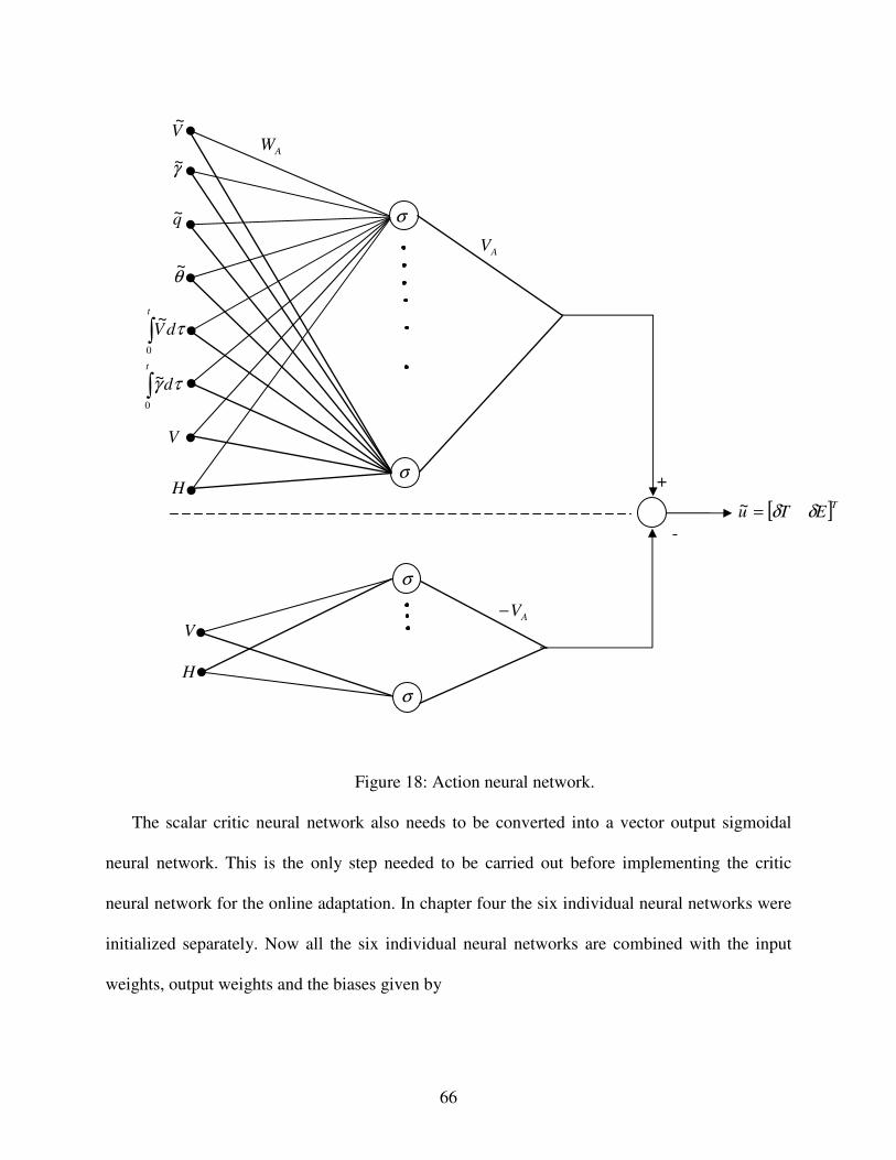
66
Figure 18: Action neural network.
The scalar critic neural network also needs to be converted into a vector output sigmoidal
neural network. This is the only step needed to be carried out before implementing the critic
neural network for the online adaptation. In chapter four the six individual neural networks were
initialized separately. Now all the six individual neural networks are combined with the input
weights, output weights and the biases given by
+
-
σ
σ
σ
σ
V~
γ~
q~
θ~
τdV
t
∫0
~
τγ d
t
∫0
~
V
V
H
H
AW
AV
AV−
[ ]TETu δδ=~
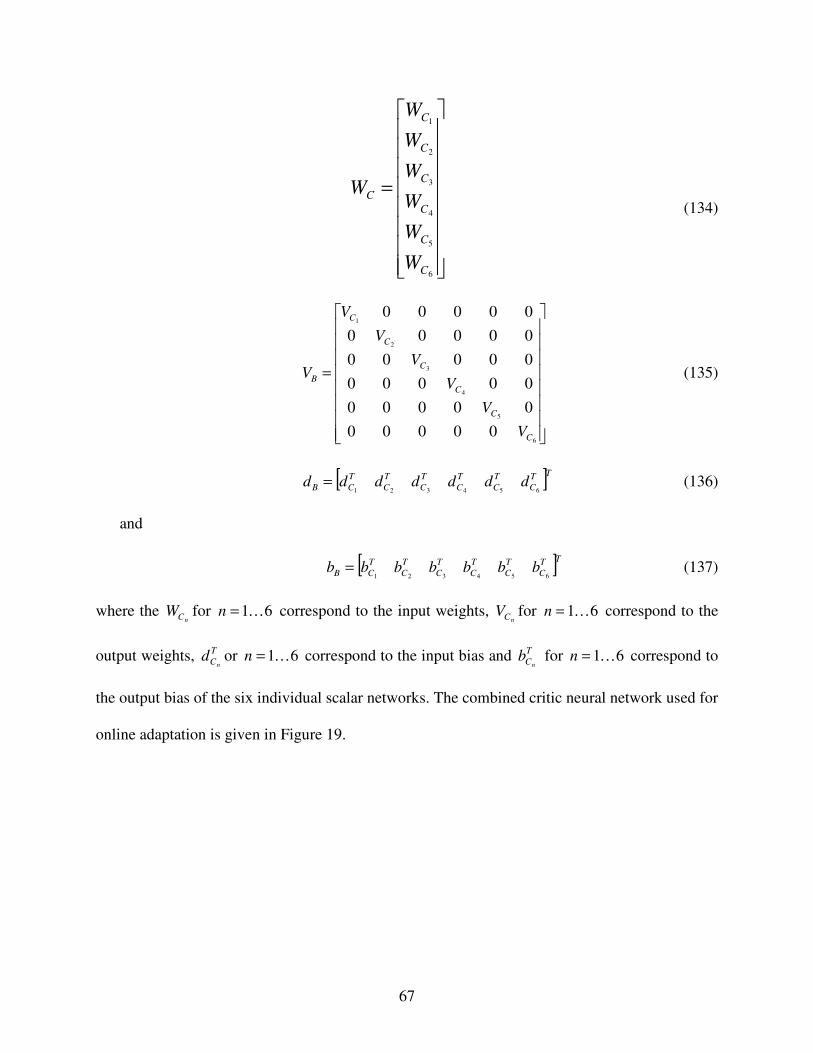
67
=
6
5
4
3
2
1
C
C
C
C
C
C
C
W
W
W
W
W
W
W (134)
=
6
5
4
3
2
1
00000
00000
00000
00000
00000
00000
C
C
C
C
C
C
B
V
V
V
V
V
V
V (135)
[ ]TT
C
T
C
T
C
T
C
T
C
T
CB ddddddd654321
= (136)
and
[ ]TT
C
T
C
T
C
T
C
T
C
T
CB bbbbbbb654321
= (137)
where the nCW for 61K=n correspond to the input weights,
nCV for 61K=n correspond to the
output weights, T
Cnd or 61K=n correspond to the input bias and T
Cnb for 61K=n correspond to
the output bias of the six individual scalar networks. The combined critic neural network used for
online adaptation is given in Figure 19.

68
Figure 19: Critic neural network.
The action and the critic neural network that approximate the optimal control law and the
gradient of the value function respectively are used in the online adaptation. The initialized
action and critic neural network are adapted online to learn new system dynamics as they arise.
The adaptation of the neural networks online is explained in the next section.
+
-
σ
σ
σ
σ
V~
γ~
q~
θ~
τdV
t
∫0
~
τγ d
t
∫0
~
V
V
H
H
CW
CV
CV−
T
t
t
a
d
V
dV
V
V
q
V
VV
V
x
V
∂
∂
∂
∂∂
∂∂
∂∂
∂∂
∂
=∂
∂
∫
∫
0
0
~
~
~
~
~
~
τγ
τ
θ
γ

69
5.3 Online adaptation
The initialized neural networks are adapted online during every time interval kk ttt −=∆ +1
based on the actual state of the aircraft to more closely approximate the globally optimal control
law. The adaptation is based on dual heuristic dynamic programming with the action network
approximating the control law and the critic evaluating the gradient of the value function. This
section describes the online adaptation algorithm for both the action and critic neural network.
The action neural network parameters are updated to minimize the mean squared error
between the desired target, )(~ tuD , and the actual output of the action network. The desired target
for the action network is given by solving the optimality condition
0)(~)(
)()(~
],~,[
)(~],[ 1
1 =∂
∂+
∂
∂=
∂
∂ ++
k
kaka
k
kaD
k
ka
tu
txt
tu
tuxL
tu
txVλ (138)
This is a set of nonlinear equations which is solved numerically using the MATLAB function
fsolve. The initial guess, G
kD tu )(~ , used in the solution of these equations is the output of the
action network with the weights from the previous time step. The algorithm for updating the
action network is shown in Figure 20. The derivative of the Lagrangian is found analytically
given by
ak
T
ak
T
a
k
kaSD RtuMtxtu
tuxL)(~)(
)(~],~,[
+=∂
∂ (139)
The discrete equivalent of the system model given by
],~,[)( 1 kaaDka tuxftx =+ (140)
is used to determine the transition matrix)(~)( 1
k
ka
tu
tx
∂
∂ + . The system model is also necessary to find
the output of the critic network )( 1+ka tλ with the weights of the critic network being equal to that

70
during the previous time step. Once the optimality condition is solved to obtain the target for the
action network i.e. )(~kD tu , the weights of the action network are now adapted using the modified
resilient back propagation algorithm.
Figure 20: Action network adaptation.
Given the state, )( ktax , guess
desired control, )(~kD tu
Compute utility function
derivative, )(~][ ktuDL ∂•∂
Use plant model for
State prediction, )1( +ktax and
transition matrix
)(~)1( ktuktax ∂+∂
Predict cost to go using
previous critic network
Predict cost to go using
previous critic network
Check stopping
condition
Update action weights
based on )(~ktDu
Perturb control guess )(~ktDu
Stop
Continue

71
Once the action network is updated, the desired output of the critic )( kaD tλ is computed
based on the current state of the system )( ka tx . The critic updating algorithm is as shown in
Figure 21. The output of the critic network is given by
)(
)]([~
)(~)(
)()(
)()(
)(
)]([~
)(~],~,[
)(
],~,[
)(
],[)( 1
11
1
ka
k
k
kaka
ka
kaka
ka
k
k
kaD
ka
kaD
ka
kakaD
tx
txu
tu
txt
tx
txt
tx
txu
tu
tuxL
tx
tuxL
tx
txVt
∂
∂
∂
∂+
∂
∂+
∂
∂
∂
∂+
∂
∂=
∂
∂≡ +
++
+ λλλ (141)
Figure 21: Critic network adaptation.
The derivative of the Lagrangian with respect to the state is obtained numerically using
Given the actual state, )( ktax
Use action network to compute
)(~ktu and control gradient
Compute utility function
derivatives
Use plant model to predict
future state and transition
matrices
Predict cost to go using
previous critic network
Update critic weights based
on desired cost-to-go
Compute desired cost-to-go

72
T
kaak
T
a
ka
kaD tuMQtxtx
tuxL)](~[)(
)(
],~,[+=
∂
∂ (142)
During the adaptation of the critic the actual value of the control )(~ktu is known, hence the
control gradient can be calculated. In addition the discretized form of the system equation can be
used to obtain the transition matrices )(~)( 1
k
ka
tu
tx
∂
∂ + and )(
)( 1
ka
ka
tx
tx
∂
∂ + . Now the critic network with the
parameters from the previous time step is used to calculate )( 1+ka tλ based on the predicted value
of )( 1+ka tx obtained from the model of the plant. Once the desired output of the critic network is
obtained, )( kaD tλ , the parameters of the critic neural networks are updated using the modified
resilient back propagation algorithm.
The updating of the action and critic network is done for every time step t∆ . Since the
updating of the action and critic network is obtained from the recurrence relation of dynamic
programming, it is seen that the system converges to the optimal trajectory over time. It is also
observed that the adaptation of the networks allows the nonlinear controller to meet performance
specifications in the presence of nonlinearities as well as multiple control failures.

73
6. SIMULATION AND RESULTS
The adaptive neural network controller is used to control the three degree of freedom
simulation of the general aviation aircraft. The simulation is carried out for different command
inputs of velocity and flight path angle. The results of the simulation are observed for parameter
variations and control failures. The online adaptation of the neural network controller prevents
loss of stability of the aircraft and tracks pilot input commands.
6.1 Simulation
The adaptive neural controller is evaluated using the simulation of a three degree of
freedom general aviation aircraft. The motion of the aircraft in the longitudinal plane is
governed by the following three nonlinear differential equations [26]. The three equations
constitute the force along the x-axis, z-axis and moment about the y-axis. One more equation
called the kinematic equation which relates the pitch rate Q with the pitch angle
( )xx TA FFmgQWUm ++−=+ θsin& (143)
( )zz TA FFmgQUWm +++=− θcos& (144)
TAyy MMQI +=& (145)
θ&=Q (146)
The aerodynamic forces and moments in equations (143), (144) and (145) can be written in terms
of the stability derivatives. The dynamics of the aircraft are characterized by these stability
derivatives. The aerodynamic forces and moments in terms of the stability derivatives are given
by equations (146), (147) and (148).
SqCCCF LDDA kx)*( 2
0+−= (147)

74
( )eZZZZZAeqZ
CQCCCCSqF δααδαα
++++= ˆˆ0
&&
(148)
( )emmmmmAeq
CQCCCCcSqM δααδαα
++++= ˆˆ0
&&
(149)
where q is the dynamic pressure, S is the reference area of the wing and c is the chord length.
The aircraft is then simulated by integrating the non linear equations of motion in the MATLAB
environment numerically. The equations of motion are integrated using the fourth order runge-
kutta method with a sampling time of 0.05 seconds. This simulation is used as the actual aircraft
in the evaluation of the adaptive critic neural network controller. The controller is evaluated for
unanticipated control failures as well as for parameter variations. The adaptive critic algorithm is
also evaluated in the presence of nonlinearity at velocities close to the stall velocity. The code
used for simulations of the adaptive critic algorithm had a limitation in that it only accepted step
input commands as well as modeling errors could only be simulated at time 0=t . Also for all
the cases other than the case near stall, the altitude of the aircraft is not shown because the
altitude remains constant.
6.2 Results
Case 1: Adaptive control during partial elevator failure
The capability of the neural network based adaptive control system to adapt to partial
elevator failure is considered first. The aircraft is initially flying at
)3000,23.181(),( 1
00 ftftshV−= , which is an interpolation point. A step input of two degrees in
flight path angle is commanded at time 0=t . A partial elevator failure is simulated by changing
the parameterE
mCδ
and E
LCδ
by 10% at time 0=t . The response of the neural network controller
is first evaluated when the neural networks are not adapted online i.e the PINN controller. The
response of the initialized neural network without adaptation is shown in Figures 22 and 23.

75
Figure 22 is a plot of velocity V ,with respect to time, t , and Figure 23 is a plot of throttle
setting, %Tδ , versus time t . As shown in Figures 22 and 23, the dynamic response of the aircraft
with PINN controller deteriorates in the presence of partial elevator failure as can be seen from
the slightly increased overshoot but with an increased settling time. The aircraft retains stability
even in the presence of partial elevator failure since LQR theory is used in the design of the
initialized controller resulting in a robust control design. In the next step, the same simulation is
carried out but the neural networks are allowed to adapt online as explained in the previous
section. The response of the neural network controller with adaptation is also shown in the same
Figures 22 and 23 with a solid line. As observed from the response we see that the overshoot in
flight path angle is reduced and the settling time is increased as compared to the PINN controller.
The action and critic neural network weights are adapted to the changed dynamics of the aircraft
due to partial failure in the elevator. The incremental cost J is also shown in figure 25, As
observed from the plots the incremental cost associated with the adaptive critic is less than that
of the PINN controller during the transient phase of the response. As the response reaches steady
state value we see a ramp in the incremental cost associated with the adaptive critic, this is due to
the steady state error associated with the adaptive critic designs.
-1 0 1 2 3 4 5 6 7 8 9 10175
176
177
178
179
180
181
182
183
184
185
Time [s]
Ve
loc
ity
[ft
/s]
Adaptive Critic
PINN
Command
-1 0 1 2 3 4 5 6 7 8 9 100
0.1
0.2
0.3
0.4
0.5
0.6
0.7
0.8
0.9
1
Time [s]
Th
rott
le [
%]
Adaptive critic
PINN

76
Figure 22: Velocity response and throttle setting for partial elevator failure.
-1 0 1 2 3 4 5 6 7 8 9 10-0.5
0
0.5
1
1.5
2
2.5
3
Time [s]
Ga
mm
a [
de
g]
Adaptive Critic
PINN
Command
-1 0 1 2 3 4 5 6 7 8 9 10-7
-6
-5
-4
-3
-2
-1
0
Time [s]E
lev
ato
r d
efl
ec
tio
n [
de
g]
Adaptive Critic
PINN
Figure 23: Flight path angle response and elevator deflection for partial elevator failure.
-1 0 1 2 3 4 5 6 7 8 9 102
2.5
3
3.5
4
4.5
5
5.5
6
Time [s]
Alp
ha
[D
eg
]
PINN
Adaptive Critic
-1 0 1 2 3 4 5 6 7 8 9 102
3
4
5
6
7
8
Time [s]
Th
eta
[D
eg
]
Adaptive Critic
PINN
Figure 24: Angle of attack and pitch angle for partial elevator failure.

77
0 1 2 3 4 5 6 7 8 9 100
10
20
30
40
50
60
Time [s]
Co
st
Adaptive Critic
PINN
Figure 25: Incremental cost for partial elevator failure.
Case 2: Adaptive control during partial thrust failure
The capability of the neural network based adaptive control system to a sudden loss of
thrust is evaluated. As in the previous simulation, the aircraft is initially flying at
)3000,23.181(),( 1
00 ftftshV−= . A step increase of five feet per second in velocity is introduced
to the system. A partial throttle gearing failure is simulated by reducing the available thrust by
10%. The response of the neural network controller is then evaluated when the neural networks
are not adapted online. The response of the initialized neural network without adaptation is as
shown as a dotted line in Figures 26 and 27. As observed from the plots, the aircraft takes longer
to settle at the pilot input command for velocity and also results in a slightly larger overshoot.
The same simulation is now carried out but the neural networks are allowed to adapt online. The
response of the neural network controller with online adaptation is also shown as a solid line in
Figures 26 and 27. As observed from the response the overshoot is slightly reduced as compared
to that of the initialized neural network controller in the presence of partial throttle gearing
failure but it also results in a slightly smaller settling time as compared to the initialized
controller. . The incremental cost J is also shown in figure 29, As observed from the plots the

78
incremental cost associated with the adaptive critic is less than that of the PINN controller during
the transient phase of the response. As the response reaches steady state value we see a ramp in
the incremental cost associated with the adaptive critic, this is due to the steady state error
associated with the adaptive critic designs
0 2 4 6 8 10 12 14 16 18 20175
180
185
190
195
Time [s]
Ve
loc
ity
[ft
/s]
Adaptive Critic
PINN
Command
0 2 4 6 8 10 12 14 16 18 200
0.1
0.2
0.3
0.4
0.5
0.6
0.7
0.8
0.9
1
Time [s]
Th
rott
le [
%]
PINN
Adaptive Critic
Figure 26: Velocity response and throttle setting for partial thrust failure.
0 2 4 6 8 10 12 14 16 18 20-4
-3
-2
-1
0
1
2
3
4
Time [s]
Ga
mm
a [
de
g]
Adaptive Critic
PINN
data3
0 2 4 6 8 10 12 14 16 18 20-5
-4.5
-4
-3.5
-3
-2.5
-2
-1.5
-1
-0.5
0
Time [s]
Ele
va
tor
De
fle
cti
on
[d
eg
]
Adaptive Critic
PINN
Figure 27: Flight path angle response and elevator deflection for partial thrust failure.

79
0 2 4 6 8 10 12 14 16 18 200
1
2
3
4
5
6
Time [s]
Alp
ha
[D
eg
]
PINN
Adaptive Critic
0 2 4 6 8 10 12 14 16 18 200
1
2
3
4
5
6
Time [s]
Th
eta
[D
eg
]
Adaptive Critic
PINN
Figure 28: Angle of attack and pitch angle for partial thrust failure.
0 2 4 6 8 10 12 14 16 18 200
500
1000
1500
2000
2500
3000
Time [s]
Co
st
Adaptive Critic
PINN
Figure 29: Incremental cost for partial thrust failure.
Case 3: Adaptive control during parameter variations
The capability of the neural network based adaptive control system is now evaluated for
modeling error between the assumed and the actual model. The aircraft is initially flying at
)3000,23.181(),( 1
00 ftftshV−= . A step input of two degrees in flight path angle is commanded at
t=0. The parameters αmC and
qmC are changed by 10% to simulate modeling error between the
aircraft and the assumed model. The response of the initialized neural network controller is
evaluated in this scenario. The response of the initialized neural network without adaptation is as

80
shown with a dotted line in Figures 30 and 31. As observed from the response of the initialized
controller the overshoot in the response of the flight path angle increases as compared to the
response with the ideal model. The same simulation is now carried out but the neural networks
are allowed to adapt online. The response of the neural network controller that is adapted online
is also shown in Figures 30 and 31 as a solid line. As observed from the response we see that the
overshoot in the flight path angle is smaller as compared to that of the initialized controller in the
presence of the modeling error. However we see an increase in settling time as compared to the
initialized controller. . The incremental cost J is also shown in figure 33, As befor the
incremental cost associated with the adaptive critic is less than that of the PINN controller during
the transient phase of the response. As the response reaches steady state value we see a ramp in
the incremental cost associated with the adaptive critic, this is due to the steady state error
associated with the adaptive critic designs
-1 0 1 2 3 4 5 6 7 8 9 10175
180
185
190
Time [s]
Ve
loc
ity
[ft
/s]
Adaptive Critic
PINN Controller
Command
-1 0 1 2 3 4 5 6 7 8 9 100
0.1
0.2
0.3
0.4
0.5
0.6
0.7
0.8
0.9
1
Time [s]
Th
rott
le [
%]
Adaptive Critic
PINN
Figure 30: Velocity response and throttle setting for variation inαmC and
qmC .

81
-1 0 1 2 3 4 5 6 7 8 9 10-0.5
0
0.5
1
1.5
2
2.5
3
Time [s]
Ga
mm
a [
de
g]
Adaptive Critic
PINN
Command
-1 0 1 2 3 4 5 6 7 8 9 10-7
-6
-5
-4
-3
-2
-1
0
Time [s]
Ele
va
tor
de
fle
cti
on
[d
eg
]
Adaptive Critic
PINN
Figure 31: Flight path angle response and elevator deflection for variation inαmC and
qmC .
-1 0 1 2 3 4 5 6 7 8 9 102
2.5
3
3.5
4
4.5
5
5.5
6
6.5
7
Time [s]
Alp
ha
[D
eg
]
PINN
Adaptive Critic
-1 0 1 2 3 4 5 6 7 8 9 102
3
4
5
6
7
8
Time [s]
Th
eta
[D
eg
]
Adaptive Critic
PINN
Figure 32: Angle of attack and pitch angle for variation in
αmC and qmC .

82
0 1 2 3 4 5 6 7 8 9 100
50
100
150
200
250
Time [s]
Co
st
Adaptive Critic
PINN
Figure 33: Incremental cost for variation inαmC and
qmC .
Next the neural network based adaptive control system is evaluated for a different
modeling error between the assumed and the actual model. The aircraft is initially flying at
)3000,23.181(),( 1
00 ftftshV−= . A step increase of five feet per second in velocity is
commanded. The parameter kDC is decreased by 10%. The response of the initialized neural
network controller is evaluated in this scenario. The response of the initialized neural network
without adaptation is as shown in Figures 34 and 35. As observed from the plots the aircraft
response has deteriorated in the presence of modeling error between the actual aircraft and the
assumed model. The same simulation is now carried out but the neural networks are allowed to
adapt online. The response of the neural network controller that is adapted online is also shown
in Figure 34 and Figure 35. As observed from the response the online adaptation of the neural
network reduces overshoot but results in a slightly larger settling time. . The incremental cost
J is also shown in figure 37, The incremental cost associated with the adaptive critic is less than
that of the PINN controller during the transient phase of the response. As the response reaches

83
steady state value we see a ramp in the incremental cost associated with the adaptive critic, this is
due to the steady state error associated with the adaptive critic designs
0 5 10 15 20 25-2
-1.5
-1
-0.5
0
0.5
1
1.5
2
Time [s]
Ga
mm
a [
de
g]
Adaptive Critic
PINN
Command
0 5 10 15 20 25-5
-4.5
-4
-3.5
-3
-2.5
-2
-1.5
-1
-0.5
0
Time [s]
Ele
va
tor
De
fle
cti
on
[d
eg
]
Adaptive Critic
PINN
Figure 34: Flight path angle response and elevator deflection for variation inkDC .
0 5 10 15 20 25180
181
182
183
184
185
186
187
188
189
190
Time [s]
Ve
loc
ity
[ft
/s]
Adaptive Critic
PINN
Command
0 5 10 15 20 250
0.1
0.2
0.3
0.4
0.5
0.6
0.7
0.8
0.9
1
Time [s]
Th
rott
le [
%]
Adaptive Critic
PINN
Figure 35: Velocity response and throttle setting for variation inkDC .

84
0 5 10 15 20 252
2.5
3
3.5
4
4.5
5
Time [s]
Alp
ha
[D
eg
]Adaptive Critic
data2
0 5 10 15 20 250
1
2
3
4
5
6
Time [s]
Th
eta
[D
eg
]
PINN
Adaptive Critic
Figure 36: Angle of attack and pitch angle for variation in
kDC .
0 5 10 15 20 250
100
200
300
400
500
600
700
800
Time [s]
Co
st
Adaptive Critic
PINN
Figure 37: Incremental cost for variation in
kDC .
Case 4: Adaptive control near stall
The capability of the neural network based adaptive control system is now evaluated for
large inputs close to the stall. The aerodynamic model of the Bonanza was modified to include
the stall model in the lift curve. The stall model incorporated is different than the actual stall of
the Bonanza, with the stall velocity much greater than the stall velocity of the actual Bonanza. In
the stall model used in this thesis, the stall angle of attack stallα was set to nine degrees, which

85
resulted in a stall velocity of 1135 −fts (80 Knots). Initially, the aircraft is flying at
)3000,23.181(),( 1
00 ftftshV−= . A step input of minus forty feet per second in velocity is
commanded at t=0. The response of the initialized neural network controller is evaluated in this
scenario. The response of the initialized neural network without adaptation is as shown with a
dotted line in Figures 38 and 39. As observed from the response of the initialized controller the
aircraft stalls and is unable to maintain the commanded airspeed. The same simulation is now
carried out but the neural networks are allowed to adapt online. The response of the neural
network controller that is adapted online is also shown in Figures 38 and 39 as a solid line. As
observed from the response we see that the adaptation prevents the aircraft from becoming
unstable and tracks pilot input command. The initialized PINN controller fails in this scenario
due the non-linearity of the drag and lift becoming significant at low speeds near stall which is
far from the initial trim velocity. As seen from the plot of incremental cost over time, we see that
the cost associated with the adaptive critic controller is less than the PINN controller.
0 5 10 15 20 25120
130
140
150
160
170
180
190
Time [s]
Ve
loc
ity
[ft
/s]
PINN
Adaptive critic
Command
0 5 10 15 20 25-0.1
0
0.1
0.2
0.3
0.4
0.5
0.6
0.7
0.8
0.9
Time [s]
Th
rott
le [
%]
Figure 38: Velocity response and throttle setting for a command of -40 ft/s in velocity.

86
0 5 10 15 20 25-8
-6
-4
-2
0
2
4
6
Time [s]
Ga
mm
a [
de
g]
PINN
Adaptive Critic
Command
0 5 10 15 20 25-14
-12
-10
-8
-6
-4
-2
0
Time [s]
Ele
va
tor
[de
g]
Figure 39: Flight path angle response and elevator deflection for a command of -40 ft/s in
velocity.
0 5 10 15 20 250
5
10
15
20
25
Time [s]
Alp
ha
Adaptive Critic
PINN
0 5 10 15 20 25-2
0
2
4
6
8
10
12
14
16
Time [s]
Th
eta
[d
eg
]
Adaptive Critic
PINN
Figure 40: Angle of attack and theta time history for a command of -40 ft/s in velocity.

87
0 5 10 15 20 252500
2600
2700
2800
2900
3000
3100
3200
3300
3400
3500
Time [s]
Altit
ude [
ft]
Adaptive Critic
PINN
Figure 41: Altitude time history for a command of -40 ft/s in velocity.
0 5 10 15 20 250
0.5
1
1.5
2
2.5
3
3.5x 10
5
Time [s]
Cost
Adaptive Critic
PINN
Figure 42: Incremental cost for a command of -40 ft/s in velocity.
In this chapter the performance of the adaptive critic based controller is evaluated using
simulations of the Bonanza. From the results it is seen that the adaptive critic controller results in
a slight reduction in overshoot as compared to the initialized controller in the presence of
unanticipated control failures and modeling errors. From the plots for modeling errors it is
observed that the PINN controller works well in the linear region of the flight envelope. In order
to test the PINN controller in the nonlinear region of the flight envelope a case near stall velocity
of the aircraft is considered. For the case near stall, it is seen that the adaptive critic controller

88
follows pilot input command of velocity where as the PINN controller is unable to maintain the
commanded value. At velocity close to the stall velocity, it is observed that the PINN
controller’s response diverges with time.

89
7. CONCLUSION
The objective of this thesis is to develop a neural network based adaptive controller for a
general aviation aircraft. A systematic method is developed for designing the neural network
based adaptive controller. Linear control theory is used to determine the architecture and the
initial weights of the neural networks in what is called the initialization phase. The initialized
neural networks meet performance specifications of the linear controller that they replace. In the
next phase, referred to as online training phase, the neural networks are allowed to adapt online
based on actual system dynamics as they arise. The online adaptation of the neural networks
compensates for nonlinear dynamics as well as control failures and parameter variations. As
demonstrated from the numerical results, the adaptive neural network based controller adapts to
partial control failures as well as parameter variations while providing system response that is
almost identical to the optimal system response. It is also apparent is that in the normal flight
envelope for the Bonanza, the aircraft behavior is close to linear that the controller initialized to
match the linear controller gains at the design points (PINN controller) is so robust, that even in
the presence of modeling error and failures, it provides adequate handling qualities, and not
much adaptation is required from the adaptive critic algorithm. In the non-linear regime of the
Bonanza, at velocities close to stall, it is observed that the PINN controller becomes unstable
whereas the adaptive critic algorithm adapts for the non-linearity and retains stability.
Comparing the dynamic inverse method with the adaptive critic method of this thesis shows that
the dynamic inverse method compensates faster for parameter variations and control failures than
the adaptive critic methodology but the PINN controller of the adaptive critic method is much
more robust in the presence of failures that the dynamic inverse method, both with adaptation
turned off. This may impact which controller can be certified for general aviation aircraft.

90
The main recommendation for future work is to evaluate the method proposed in this
thesis to various other practical systems. Another important area of research could focus on using
a different approach in the design of the linear controller. Since optimal estimation problem is
seen as a dual of the optimal control problem, a logical step would be to expand the process
proposed in this design to the development of a near optimal estimator. The initialization of the
neural networks could be based on Kalman gains obtained at different operating points. Future
work could also be focused on proofs for the stability and robustness of the neural network
learning algorithm.

91
REFERENCES

92
REFERENCES
[1] Suresh, S, Omkar, S.N, Mani, V and Sundarajan, S, “Direct Adaptive Neural Flight
Controller for F-8 Fighter Aircraft.” Journal of guidance, control and dynamics Vol. 29, No. 2,
pp. 454-464, March–April 2006.
[2] Kim, Byoung and Calise, Anthony, “Nonlinear Flight Control Using Neural Networks.”
Journal of guidance, control and dynamics, Vol. 20, No. 1, pp. 26-33, January–February 1997.
[3] Rysdyk, Rolf and Calise, Anthony, “Adaptive Model Inversion Flight Control for Tiltrotor
Aircraft”, American helicopter society annual forum, Washington D.C, May 1998.
[4] Perhinschi, M.G., Napolitano, M.R., Campa, G., Fravolird, M.L., Massotti, L., Lando, M.
“Augmentation of a non linear dynamic inversion scheme within the NASA IFCS F-15 WVU
simulator”, American Control Conference, 2003. Proceedings of the 2003, Volume 2, Issue, June
4-6, 2003 Page(s): 1667 – 1672.
[5] Gundy-Burlet, Karen, Krishnakumar, K, Limes, Greg and Bryant, Don, “Augmentation of an
Intelligent Flight Control System for a Simulated C-17 Aircraft.” Journal of Aerospace,
Computing, Information and Communication, Vol. 1, pp. 526-542, December 2004.
[6] Steck, James E., Pesonen, Urpo J., Rokhsaz, Kamran, Bruner, Hugh Samuel and Duerksen,
Noel, “Adaptive Neural Network Inverse Controller for General Aviation Safety.” Journal of
guidance, control and dynamics, Vol. 27, No. 3, pp. 434-443, May–June 2004.
[7] Steck, James E., Pesonen, Urpo J., Rokhsaz, Kamran, Singh, Balbahadar and Chandramohan,
Rajeev “Effect of Turbulence on an Adaptive Dynamic Inverse Flight Controller.”
Infotech@Aerospace,26 - 29 September 2005, AIAA-2005-7038, Arlington, Virginia
[8] Rokhsaz, Kamran, Steck, James E., Singh, Balbahadar and Chandramohan, Rajeev
“Response of An Advanced Flight Control System to Microburst Encounters” 2005 Transactions
Journal of Aerospace, SAE, pp.1432-1441.
[9] Kulkarni, Nilesh and Phan, Minh, “A Neural Network Based Design of Optimal Controllers
for Nonlinear Systems.” AIAA Guidance, Navigation, and Control Conference and Exhibit 5-8
AIAA-2002-46884, August 2002, Monterey, California.
[10] Balakrishnan, S.N and Biega, Victor, “Adaptive-Critic-Based Neural Networks for Aircraft
Optimal Control.” Journal of guidance, control and dynamics Vol. 19, NO. 4, pp. 893-898, July-
August 1996.
[11] Saini, G., Balakrishnan, S.N., Person, C., “Adaptive critic based neurocontroller for
autolanding of aircraft with varying glideslopes.” International conference on neural networks,
Vol. 4, pp. 2288 – 2293, 1997.

93
[12] Shin, Yoonghyun, Johnson, Matthew D., Calise, Anthony J, “Neural Network-Based
Adaptive Control for Nonlinear Flight Regimes”, AIAA Guidance, Navigation and Control
Conference, AIAA-2003-5717, August 2003.
[13] Williams-Hayes, Peggy, “Flight Test Implementation of a Second Generation Intelligent
Flight Control System”, infotech@Aerospace, AIAA-2005-6995, 26-29 September 2005,
Arlington, Virginia.
[14] Ferrari, Silvia and Stengel, Robert “Online Adaptive Critic Flight Control.” Journal of
guidance, control and dynamics, Vol. 27, No. 5, pp. 777-786, September–October 2004.
[15] Bellman, R. E., “Dynamic Programming”, Princeton University Press, Princeton, NJ,
1957.
[16] Ferrari, Silvia “Algebraic and Adaptive Learning in Neural Control Systems”, Dissertation,
Princeton, November 2002.
[17] Prokhorov, D. and Wunsch, D. “Adaptive Critic Designs,” IEEE Trans. on Neural
Networks, Vol. 8, No. 5, pp. 997-1007, 1997.
[18] Burl, Jeffrey B. “Linear Optimal Control H2 and H ∞ Methods”, Addison Wesley, 1999.
[19] Howard, R., “Dynamic Programming and Markov Processes”, MIT Press, Cambridge, MA,
1960.
[20] Ferrari, Silvia and Stengel, R.F. “Classical/Neural Synthesis of Nonlinear Control Systems”,
Journal of Guidance, Control, and Dynamics, Vol. 25, No. 3, May-June 2002.
[21] Ferrari, Silvia and Stengel, R.F. “Smooth Function Approximation using Neural Networks”,
IEEE Transactions on Neural Networks, Vol.16, No. 1, January 2005.
[22] Stengel, R. F., “Flight Dynamics”, Princeton University Press, 2004.
[23] Huang, C. and Stengel, R. F. “Restructurable Control Using Proportional-Integral Model
Following,” Journal of Guidance, Control, and Dynamics, Vol. 13, No. 2, pp. 303-309, 1990.
[24] Nelson, R. C., “Flight Stability and Automatic Control”, McGraw-Hill, Inc., New York,
NY, 1989.
[25] Stengel, R. F., “A Unifying Framework for Longitudinal Flying Qualities Criteria,” Journal
of Guidance, Control, and Dynamics, Vol. 6, No. 2, pp. 84-90, 1983.
[26] Roskam, Jan, “Airplane Flight Dynamics and Automatic Flight Controls.” DARcorporation,
2003.