Embed Size (px)
Citation preview

Adaptive Boosting for Synthetic Aperture Radar
Automatic Target Recognition
Yijun Sun, Zhipeng Liu, Sinisa Todorovic, and Jian Li∗
Department of Electrical and Computer Engineering
University of Florida, P.O. Box 116130
Gainesville, FL 32611-6130
Abstract: We propose a novel automatic target recognition (ATR) system for classification
of three types of ground vehicles in the MSTAR public release database. First, MSTAR image
chips are represented as fine and raw feature vectors, where raw features compensate for the
target pose estimation error that corrupts fine image features. Then, the chips are classified by
using the adaptive boosting (AdaBoost) algorithm with the radial basis function (RBF) network
as the base learner. Since the RBF network is a binary classifier, we decompose our multiclass
problem into a set of binary ones through the error-correcting output codes (ECOC) method,
specifying a dictionary of code words for the set of three possible classes. AdaBoost combines
the classification results of the RBF network for each binary problem into a code word, which is
then “decoded” as one of the code words (i.e., ground-vehicle classes) in the specified dictionary.
Along with classification, within the AdaBoost framework, we also conduct efficient fusion of the
fine and raw image-feature vectors. The results of large-scale experiments demonstrate that our
ATR scheme outperforms the state-of-the-art systems reported in the literature.
Keywords: MSTAR, automatic target recognition, adaptive boosting, feature fusion
IEEE Transactions on Aerospace and Electronic Systems
Submitted in December 2004. Accepted in March 2006
∗Please address all correspondence to: Dr. Jian Li, Department of Electrical and Computer Engineering, P.
O. Box 116130, University of Florida, Gainesville, FL 32611, USA. Phone: (352) 392-2642. Fax: (352) 392-0044.
E-mail: [email protected].
1

1 Introduction
Radar systems are important sensors due to their all weather, day/night, long standoff capabil-
ity. Along with the development of radar technologies, as well as with increasing demands for
target identification in radar applications, automatic target recognition (ATR) using synthetic
aperture radar (SAR) has become an active research area. The latest theoretical developments
in classification methodologies quickly find applications in the SAR ATR design. Joining these
efforts, in this paper, we present a new ATR scheme based on the adaptive boosting (AdaBoost)
algorithm [1], which yields the best classification results reported to date in the literature on the
MSTAR (Moving and Stationary Target Acquisition and Recognition) public release database.
The MSTAR data is a standard dataset in the SAR ATR community, allowing researchers to
fairly test and compare their ATR algorithms. The literature abounds with reports on systems
where the MSTAR database is used for validation. Among these systems, one most commonly
used approach is the template based method [2, 3, 4]. In this method, for each class, a set of filters
(templates) is generated to represent target signatures around different aspect angles; then, a
given target is identified as the class whose filters give the “best” output. The template based
method, however, is computationally inefficient. Here, high classification accuracy conditions
the create of large sets of filters for each class, which results in extensive computation both in
the training and testing stages. In addition, large memory-storage requirements, inherent to the
method, are a major hindrance for its implementation in systems subject to stringent real-time
constraints.
A more appealing approach is to design a classifier, which can be represented by a set of
parameters. For example, in [5], the authors use the neural network for their ATR system. Its
parameters can be easily estimated through optimization of a specified cost function, as for ex-
ample in the back-propagation algorithm. However, the neural network is prone to overfitting.
Moreover, after training of the neural network, its parameter estimates are not guaranteed to be
a global-minimum solution of a given optimization function. Recently developed large-margin
based algorithms have been reported to successfully alleviate the overfitting problem, while at
the same time maintaining the classification efficiency. Two typical examples of the margin-based
classifiers are the support vector machine (SVM) [6] and AdaBoost [1]. Interestingly, SVM-based
ATR systems (e.g., [7, 8]) perform only slightly better than the template based approaches. Con-
cerning AdaBoost, the literature reports success of many AdaBoost-based systems for pattern
classification (e.g., [9, 10]). Nevertheless, to our knowledge, it has not yet gained appropriate
attention in the SAR ATR community.
In this paper, we propose a novel classification scheme for the MSTAR data using the
2
AdaBoost algorithm. The most important property of AdaBoost is its ability to find a highly
accurate ensemble classifier by combining a set of moderately accurate member classifiers, called
hypotheses or base learners. AdaBoost guarantees an exponential decrease of an upper bound
of the training error with the increase in the number of hypotheses, subject to a mild con-
straint that each base hypothesis achieves an error rate less than 0.5. Moreover, both theoretical
and empirical results demonstrate that AdaBoost has an excellent generalization performance
[11, 12].
AdaBoost is originally designed for a binary classification problem. To categorize multiple
types of vehicles in the MSTAR database, we first employ the error-correcting output codes
(ECOC) method [13], to decompose the multiclass problem into a set of binary sub-problems.
We refer to this decomposition as coding scheme, where each class is labeled with a code word.
Then, for each binary problem, we build a binary classifier by using AdaBoost with the radial
basis function (RBF) network [14] as the base learner. When presented an unseen sample, each
binary classifier produces a bit in a code word, which is then classified measuring the distance
of that code word from the code words in the dictionary specified by the coding scheme. The
experimental results, reported herein, show that the outlined classification system, without any
preprocessing of the MSTAR data, achieves comparable performance to that of systems utilizing
sophisticated pose estimators. This means that our SAR ATR system can be implemented
for the applications with stringent real-time constraints, where estimation of target poses is
computationally prohibitive.
The performance of the outlined system can be further improved by accounting for the
randomly distributed poses of SAR image chips, ranging from 0◦ to 360◦. We propose a pose
estimation algorithm, whereby all targets are rotated to the same aspect angle. Although our
pose estimation algorithm is quite accurate, it may fail when a target is severely shadowed
and/or distorted. To compensate for the occasional pose estimation error, we represent MSTAR
images by two sets of image features. The first set, called raw features, represent pixel values
of the original image chips that are not pre-processed. The second set of features, called fine
features, comprises magnitudes of two-dimensional DFT coefficients computed on the aligned
image chips, which are rotated to the same aspect angle by the pose estimator. Here, it is
necessary to design an efficient data fusion method for combining the two highly correlated
feature sets. Again, AdaBoost lends itself as a natural solution. Essentially, we utilize AdaBoost
to choose a “better” feature set in each training iteration, such that the final ensemble classifier
is optimized over the two feature sets. The resulting classification system, which incorporates
the information from the pose estimator, can correctly classify 1360 out of 1365 testing samples,
which, to our knowledge, is the best result ever reported in the literature.
3

The paper is organized as follows. In Section 2, we present our data preprocessing, including
the pose estimation and image-feature representation. In Section 3, we give a brief review of
AdaBoost and the RBF network, as well as discuss how to use AdaBoost for feature fusion and
ultimate multiclass target recognition. Experimental results on the MSTAR data are presented
and discussed in Section 4. We conclude with our remarks on the proposed system in Section 5.
2 Data Preprocessing
2.1 Pose Estimation
Targets in the MSTAR data have randomly distributed poses, ranging from 0◦ to 360◦. Elim-
inating variations in target poses can significantly reduce the classification error. However,
accomplishing an accurate estimation of poses is a challenging task. In general, it can be con-
sidered as a regression problem, where a pose estimator maps a high dimensional data sample
(in our case, a 128×128 image chip) to a real value between 0 and 360. In comparison to the
classification problem, where only one label from a finite label space is assigned to each sam-
ple, the regression problem is usually considered more difficult. Fortunately, available a priori
knowledge can be exploited to mitigate the difficulty of the pose estimation problem.
In this paper, we assume that the MSTAR data is rectangular shaped, such that the target
pose is uniquely determined by the longer edge. The angle between the longer edge and the
horizontal image axis is defined as target pose. Therefore, by detecting the longer edge of a
given target, we can immediately compute its pose; however, with the uncertainty of 180◦ with
respect to the referent aspect angle, since the edge detection does not provide the information on
the orientation of the target. That is, after the target is rotated, for example, to be horizontally
aligned with the image boundaries, it is not known whether the target heads right or left.
Unlike in optical images, targets in SAR images do not have clear edges. To detect edges,
it is first necessary to segment targets from noisy background, and then detect edges of the
segmented targets. In Figure 1, we present a block-diagram of our edge detection procedure.
Since the radar reflection varies from chip to chip, we first equalize the intensity of the image
to be in the interval from 0 to 1, by using the standard histogram equalization method [15].
Histogram equalization modifies the dynamic range and contrast of an image by employing a
monotonic, non-linear mapping which re-assigns the intensity values of pixels in the input image,
such that the output image contains a uniform distribution of intensities. Then, to the equalized
image chip, we apply a mean filter, which reduces the image noise level. The “smoothed” image
is then roughly segmented with a predefined threshold θ1. As output, we obtain a roughly
4
segmented target with pixel values larger than θ1. Next, the median of this target is calculated.
The median, denoted as θ2, is used as a threshold for the subsequent fine-target segmentation.
From our experiments, the median is more appropriate as a threshold than the mean of target
pixel values, because the mean can be strongly influenced by extremely high pixel values, larger
than θ1, that are usually noise artifacts. After the fine-target segmentation, target edges are
detected by using the standard Sobel filter [15], and then dilated with a d2×d2 box. In Figure
2, we depict an example of the outlined edge-detection procedure for a T72 target. In our
experiments, we set the parameters to the following values: θ1 = 0.8 and d2 = 2.
The above algorithm poorly detects straight edges for majority of the chips. To alleviate this
problem, we perform an exhaustive target-pose search over different pose angles. Thus, for each
pose angle α, we first draw a rectangle in α direction, such that the sides of the rectangle are
tangent to the detected target contour, as depicted in Figure 3. Here, α is the angle between
the longer side of the rectangle and the horizontal image axis, as illustrated in Figure 3. Then,
we dilate the sides of the rectangle to be d2 pixels wide. Next, along the two longer sides of
the rectangle, we compute the number of pixels that belong to both the target contour and the
rectangle sides, and find the maximum of the two numbers. The maximum number of overlapped
pixels is recorded as the edge weight in α direction, w(α). This procedure is iterated, rotating
the tangent rectangle with a rotation step ∆α, until the entire interval [0◦, 180◦] is covered. Since
we assume that targets have a rectangular shape, there is no need to conduct search for angles
greater than 180◦. The angle α∗, characterized by the largest edge weight, α∗ = arg maxα w(α),
is selected as the target-pose estimate.
In our experiments, we set ∆α = 5◦. To compute the pose estimation error we determine
the ground truth by human inspection. For majority of the chips, the pose estimation error is
within ±5◦. However, the method fails in some cases, where the longer target edge is shadowed
or significantly distorted, as illustrated in Figure 4. In these cases, our algorithm estimates the
angle of the shorter target edge as α∗.
To identify potential outliers, we test each estimate against the following two criteria: (1) α∗
is approximately 180◦, and (2) w(α∗) is smaller than a certain threshold. If neither is true then
the pose estimate is equal to α∗. Otherwise, if the outcome of either of these two tests is positive,
we check yet another criterion: if the target length, measured along α∗ direction, is smaller than
the target width, measured along the direction perpendicular to α∗ (see Figure 3). If the last
test is negative then we consider the pose estimate equal to α∗. If the last test is positive then
the pose estimate is equal to the angle perpendicular to α∗. In Figure 4, we illustrate the above
outlier-test procedure, where the pose estimates of the vehicles in Figure 4 are corrected to 85◦
and 60◦, respectively – the values that are very close to ground truth.
5

To validate our approach, we calculate the pose estimation error with respect to manually
estimated target poses. For three training data sets: T72 sn-132, BMP2 sn-c21, and BTR70
sn-c71, at 17◦ depression angle, the mean of the error is −0.32◦ and the standard deviation of
the error is 6.87◦. For seven test data sets: T72 sn-132/s7/812, BMP2 sn-c21/9566/9563, and
BTR70 sn-c71, at 15◦ depression angle, the mean of the error is 0.07◦ and the standard deviation
of the error is 7.82◦. Note that the standard deviation of the error is slightly greater than our
search step, ∆α=5◦, suggesting that our method is quite reliable.
2.2 Image Representation
In our approach, the MSTAR image chips are represented by two types of image-feature vectors
that we refer to as raw and fine features. The reason for representing images by two feature sets
is to reduce the occasional pose estimation error, as we discuss below.
For representing images by fine features, we use the estimated fine target pose to rotate the
target to the referent aspect angle of 180◦, as illustrated in Figure 5. Then, we crop the image by
selecting an 80×80 window in the center of the image. Next, we compute the two-dimensional
DFT for the cropped image. Finally, the magnitudes of the 2-D DFT coefficients are used as
fine features.
The well-known properties of the 2-D DFT [16] render this transform very suitable for our
purposes. More specifically, note that by using the magnitudes of 2-D DFT coefficients, we
alleviate the problem of target-center variations. The variations in target-center locations can
be viewed as image shifts along x and y coordinates. Since a shift in a 2-D signal does not change
its power spectral density (PSD), the DFT is invariant to these variations. In addition, the DFT
eliminates the inherent 180◦ uncertainty of our pose estimation algorithm, since for any signal
x(n) we have that x(−n) has the same PSD as x(n).
Relying only on the fine-feature set may cause poor classification performance, due to the
limited accuracy of our pose estimation algorithm. To compensate for the pose estimation error
in fine features, we also represent images by raw features. The raw features of a given image are
equal to individual pixel values in an 80×80 window, positioned at the center of the image.
3 Classifier Design
In our approach, each image in the MSTAR database is represented as a feature vector or
pattern. Hence, target identification can be formulated as a machine learning problem, where
unseen patterns are labeled using a trained classifier. As a classifier, in this paper, we use
6
AdaBoost. For completeness, below, we first give a brief review of AdaBoost. Then, we describe
how AdaBoost can be used as a multiclass classification method as well as a feature fusion
method.
3.1 AdaBoost
Given an unseen pattern x and a class of hypothesis functions H = {h(x) : x → R}, called weak
learners or base learners, we are interested in finding an ensemble classifier F (x), or f(x), given
by
F (x) =∑
t
αtht(x) and f(x) =1
∑
t αt
F (x), (1)
such that a certain cost function C is optimized. By optimizing C, both the combination
coefficients α = [α1, . . . , αT ], and the hypotheses ht(x), t = 1, . . . , T , are learned in the training
process on the given set of training samples D = {(xn, yn)}Nn=1 ∈ X × Y, where X is a pattern
space, and Y is a label space. For the time being, we consider the binary classification problem,
where Y = {−1, +1}.To find the ensemble function in Eq. (1), several ensemble methods have been developed
recently [1, 17, 18]. Among them, AdaBoost is considered one of the most important recent
developments in the classification methodology [1, 11, 12]. It has been shown that AdaBoost
searches for α and ht(x), t = 1, . . . , T by performing a functional gradient descent procedure on
the following cost function:
C =1
N
N∑
n=1
exp(−ynF (xn)), (2)
which is an upper bound of the empirical error Eemp = 1N
∑N
n=1 I{yn 6= sign(F (xn))}. Here,
I{·} is the indicator function, and sign(·) is the sign operator. Note that the cost function in
Eq. (2) can be expressed as
C =1
N
N∑
n=1
exp(−ynf(xn)∑
t
αt) =1
N
N∑
n=1
exp(−ρ(xn)∑
t
αt), (3)
where the sample margin is defined as ρ(xn) , ynf(xn). This motivated researchers to try to
explain the good generalization properties of AdaBoost by using the margin theory [11, 12], that
is, to relate AdaBoost to those algorithms that directly maximize the classifier margin (or simply
margin) defined as ρ , min1≤n≤N ρ(xn).
The original AdaBoost algorithm [1] uses binary-valued hypotheses, i.e., h(x) : x → {±1},as the base learners. Schapire and Single [19] extended the original AdaBoost to a more general
7

case, where real-valued hypotheses are used. Here, h(x) : x → [−1, +1], where the sign of
h(x) represents the class label assigned to the sample x, and the magnitude |h(x)| represents
the prediction “confidence”. The pseudo-code of the confidence-rated AdaBoost is presented in
Figure 6.
The main idea of AdaBoost is to repeatedly apply the base learning algorithm to the re-
sampled versions of the training data, to produce a collection of hypothesis functions, which are
ultimately combined via a weighted linear vote to form the ensemble classifier in Eq. (1). An
intuitive idea in AdaBoost is that the sample, which are misclassified, get larger weights in the
following iterations (Eq. (17)); hence, in the subsequent training steps, the base learner is forced
to focus on these hard-to-classify cases, which, for instance, are close to the decision boundary.
The weights associated with data patterns at iteration step t form the distribution over patterns,
denoted as d(t).
Initially, the probability of selecting each pattern is set to be uniform, that is, d(1)(n) = 1/N ,
n = 1, . . . , N . In each iteration, t, the base learner is trained on a dataset sampled from the orig-
inal training data based on the distribution d(t)=[d(t)(1), . . . , d(t)(N)]. Then, the performance of
the base learner, measured through the edge, defined as rt ,∑N
n=1 d(t)(n)ynht(xn), conditions
the value of the combination coefficient, αt, computed as in Eq. (16). Note that if rt is equal to
zero, there is no information that ht contributes to the ensemble classifier; therefore, αt is set to
zero. Usually, it is assumed that H is negative close; that is, if h ∈ H then −h ∈ H. Given this
assumption, we can further assume that the combination coefficients α are non-negative without
loss of generality. If αt happens to be negative in Eq. (16), −h can be used instead of h in Eq.
(1), in order to change the sign of negative rt and αt. After computing αt, the distribution d(t)
is updated, as in Eq. (17). Note that if the sign of ht(xn) agrees with yn, d(t)(n) decreases,
otherwise d(t)(n) increases.
One of the most important properties of AdaBoost is that, under a mild assumption that
weak learners can achieve the error rate less than random guessing (i.e., < 0.5), AdaBoost
exponentially reduces the training error to zero as the number of the combined base hypotheses
increases [19]. Moreover, along with minimizing the cost function C, given by Eq. (2), AdaBoost
effectively maximizes the margin of the resulting ensemble classifier. Consequently, the ensemble
classifier is characterized by small generalization error. In many cases, the generalization error
continues to decrease, with each iteration step, even after the training error reaches zero [11, 12].
8

3.2 Base Learner: RBF Network
As the base learner in AdaBoost, we use the RBF network [14]. The RBF net is a multidi-
mensional nonlinear mapping based on the distances between the input vector and predefined
center vectors. Using the same notation as in Section 3.1, the mapping is specified as a weighted
combination of J basis functions:
h(x) =
J∑
j=1
πjφj(‖x− cj‖p), (4)
where φj(‖x − cj‖p) is a radial basis function (RBF), πj is a weight parameter, and J is a
pre-defined number of RBF centers. Basis functions φj(·) are arbitrary nonlinear functions, ‖·‖p
denotes the p-norm (usually assumed Euclidean), and vectors cj represent RBF centers.
In the literature, one of the most popular RBF nets is the Gaussian RBF network [20]. Here,
the basis functions are specified as the un-normalized form of the Gaussian density function
given by
g(x) = exp
(
−1
2(x − µ)TΣ−1(x − µ)
)
, (5)
where µ is the mean and Σ is the covariance matrix. For simplicity, Σ is often assumed to have
the form Σ = σ2I. Hence, the Gaussian RBF network is given by
h(x) =
J∑
j=1
πjgj(x) =
J∑
j=1
πj exp
(
−‖x− µj‖2
2
2σ2j
)
, (6)
where the µ’s represent center vectors, while the σ’s can be interpreted as the width of basis
functions.
The parameters of the Gaussian RBF network – namely, the means {µj}, the variances {σ2j },
and the weighting parameters {πj} – are learned on training samples. In this paper, we employ
an iterative learning algorithm, where all the RBF parameters are simultaneously computed by
minimizing the following error function [21]:
E =1
2
N∑
n=1
(yn − h(xn))2 +λ
2N
J∑
j=1
π2j , (7)
where λ is a regularization constant. In the first step, the means {µj} are initialized by the
standard K-means clustering algorithm, while the variances {σj} are determined as the distance
between µj and the closest µi, (i 6= j, i ∈ [1, J ]). Then, in the following iteration steps, a
gradient descent of the error function in Eq. (7) is performed to update {µj}, {σ2j }, and {πj}.
In this manner, the network fine-tunes itself to training data.
9

3.3 Multiclass Classification
So far, we have presented the ensemble classifier capable of solving binary-class problems. Since
our goal is to identify three types of targets in the MSTAR dataset, we are faced with the
multiclass problem. Here, a label from a finite label space Y = {1, · · · , K}, K > 2, is assigned
to each pattern. To design such a classifier by using a binary classifier (in our case, AdaBoost
with RBF nets), we first decompose the multiclass problem into several binary problems. For
this purpose, one popular approach is to implement the error-correcting output codes (ECOC)
method, where each class is represented by a codeword in a suitably specified code matrix [13].
Here, each label y ∈ Y is associated with a row of a pre-defined code matrix, M ∈ {−1, +1}K×L.
Below, we denote the k-th row of M as Mk·, then, the l-th column as M·l, and finally the
(k, l)-th entry of M as Mkl. Note that the l-th column of M represents a binary partition over
the set of classes, labeled according to M·l. This partition enables us to apply a binary base
learner to multiclass data. For each binary partition (i.e., column of M), the binary base learner
produces a binary hypothesis fl. It follows that the K-class problem can be solved by combining
L binary hypotheses fl, l = 1, . . . , L. After learning L binary hypotheses, the output code of a
given unseen instance x is predicted as f(x) = [f1(x), . . . , fL(x)]. This output code is “decoded”
as label y, if the y-th row of the code matrix, My·, is “closest” to f(x) with respect to a specified
distance metric d(My·, f(x)).
A more general framework for decomposing the multiclass problem can be formulated by
using a code matrix from the following set of matrices: {−1, 0, +1}K×L [22]. Here, a zero entry,
Mkl=0, indicates that the classification of hypothesis fl is irrelevant for label k. Consequently,
fl is learned only for those samples (x, Myl) where Myl 6=0. Such definition of the code matrix
provides for a unifying formulation of a wide range of methods for decomposing the multiclass
problem, including the well-known one-against-others, and all-pair approaches [22]. For the one-
against-others scheme, M is a K×K matrix with all diagonal elements equal to +1 and all other
elements equal to −1. An example of the one-against-others code matrix for K = 3 is given in
the following equation:
Mo =
+1 −1 −1
−1 +1 −1
−1 −1 +1
. (8)
For the all-pair scheme [23], M is a K ×(
K2
)
matrix, where the number of columns is equal to
the number of distinct label pairs (k1, k2). In the column l, which is assigned to the label pair
(k1, k2), only the elements in rows k1 and k2 are nonzero. An example of the all-pair code matrix
10

for K = 3 is given in the following equation:
Ma =
+1 0 −1
−1 +1 0
0 −1 +1
. (9)
In our multiple-target classification experiments, we use both coding approaches.
Recall that for the ultimate classification it is necessary to specify the distance metric
d(My·, f(x)). One possible approach is to use the standard Hamming distance equal to the
number of bits of the output code f(x) different from those of the codeword My·. When the
Hamming distance is used, a sample x is classified as label y if
y = arg miny
L∑
l=1
1 − sign(Mylfl(x))
2, (10)
where sign(z) is defined as
sign(z) =
1 , z > 0 ,
0 , z = 0 ,
−1 , z < 0 .
(11)
A drawback of using the Hamming distance for decoding is that it does not make use of
the confidence level indicated by the magnitude of fl(x). This problem can be alleviated by
employing the Euclidean distance in conjunction with the following decoding rule:
y = argminy
‖My· − f(x)‖2, (12)
where ‖ · ‖2 is the 2-norm. If codewords are symmetrically spaced in the L-dimensional space,
as is the case in the one-against-others and all-pair methods, for all labels y, My· has the same
number of nonzero elements. In this case case, the decoding rule can be simplified as
y = arg maxy
L∑
l=1
Mylfl(x) . (13)
We refer to the decoding rule in Eq. (13) as max-correlation decoding.
3.4 AdaBoost as a Fusion Method
Recall that in our approach each MSTAR image chip is represented by two sets of image features
– namely, fine and raw features. In Section 2.2, we discuss that the reason for representing images
by raw features is to compensate for the target pose estimation error in the fine features. We
hypothesize that combining the information of both feature sets would improve the classification
performance. In the literature, a method for combining several pieces of information from various
11

sources with the goal to obtain a better performance than on each individual piece of information
is called the information fusion. In our case, we seek to combine the information contained in
the two feature sets. Since, the two feature sets are highly correlated, it is very challenging
to design a transform that would fuse the two feature sets into one in a new feature space.
Instead, we propose to use AdaBoost to combine the information from both sets, while keeping
them separate. Note that AdaBoost, here, does not transform the two feature spaces into a new
space, where the two feature sets would be united, and as such is not a typical fusion method.
However, AdaBoost combines the two sources of information improving the classification results,
as explained below, and therefore, we refer to it as fusion method.
Essentially, the idea is to choose a “better” set in each AdaBoost training iteration, such
that the final ensemble function is optimized over the two feature sets. To this end, we use a
fundamental theoretical result, presented in [19], that the upper bound of the training error in
Eq. (2) is equal to the product of the normalizing constants {Zt}, defined in Eq. (18):
1
N
N∑
n=1
I{yn 6= sign(F (xn))} 61
N
N∑
n=1
exp(−ynF (xn)) =T∏
t=1
Zt . (14)
The pseudo-code of the fusion algorithm is shown in Figure 7. There are two separate
branches of learning processes: Steps 1a-3a and Steps 1b-3b in Figure 7. In one branch the
ensemble classifier is iteratively trained on fine feature vectors xfn, and in the other, on raw
feature vectors xrn. More precisely, in each training step t, for both feature sets, the base learner
ht, combination coefficient αt, and normalization constant Zt are calculated with respect to the
data distribution d(t). Since the empirical training error is bounded by the product of {Zt} (Eq.
(14)), we choose Zt as a criterion for selecting between the two feature sets. Thus, in iteration
step t, the branch that produces smaller Zt would yield a smaller upper bound of the empirical
training error, and, as such, is selected. Then, for the following step t+1, we use ht, αt, and Zt
of the selected branch to update the data distribution d(t+1). Note that it is necessary to keep
track of the feature set used for computing each hypothesis ht in the ensemble classifier F (x).
In experiments on test images, a given base hypothesis ht should operate on the same feature
set as that selected in the training process.
The outlined strict mathematical formulation of the AdaBoost fusion algorithm has a more
appealing intuitive interpretation. Recall that AdaBoost has the capability of identifying difficult-
to-classify examples in the training data. During training, a given target sample with erroneous
pose estimation, will be categorized as a hard example, if fine features are used to represent that
sample. To prevent the propagation of pose-estimation error in AdaBoost training, we simply
discard the information of fine features and use raw features instead for those difficult-to-classify
training data.
12

4 Experimental Results
4.1 Experimental Setup
We validate the proposed ATR system on the MSTAR public release database [2]. Here, the task
is to classify three distinct types of ground vehicles: BTR70, BMP2, and T72. There are seven
serial numbers (i.e., seven target configurations) for the three target types: one BTR70 (sn-c71),
three BMP2’s (sn-9596, sn-9566, and sn-c21), and three T72’s (sn-132, sn-812, and sn-s7). For
each serial number, the training and test sets are provided, with the target signatures at the
depression angles 17◦ and 15◦, respectively. The sizes of the training and test datasets are given
in Table 1.
We conduct experiments for two different settings. In the first setting, which we refer to
as S1, our classifier is optimized by using all seven training sets and tested on all seven test
sets. To balance the number of training data per target class, we augment the training set
of BTR70 sn-c71 by triplicating each image chip. To explain the reasoning for augmenting
the training set, note that the RBF neural network tries to minimize the mean squared error:
E =1
N(
∑
{n:yn=+1}
(yn − h(xn))2 +∑
{n:yn=−1}
(yn − h(xn))2), where h(·) is a mapping function.
Consequently, if the number of training samples varies across classes, h(·) is biased towards classes
with majority population. It is a standard practice to alleviate this problem by augmenting
minority classes with sample duplicates [?],[?], so that all classes are equally populated, which
improves the accuracy of the outlined training of RBF.
In the second setting, referred to as S2, our classifier is learned using only a subset of training
data, and tested on all available test data. More precisely, for training we use training datasets
of BTR70 sn-c71, BMP2 sn-c21, and T72 sn-132, while for testing, all seven test sets. By doing
so, we are in a position to examine the generalization properties of our method.
Throughout, to reduce computational complexity, the dimensionality of each data is reduced
to 150 by principal component analysis (PCA)[24]. PCA is one of the most commonly used
dimensionality reduction method that projects pattern vectors onto a low-dimensional subspace,
so that the re-construction error is minimum in the least-square sense. The obtained low-
dimensional subspace is spanned by a selected subset of eigenvectors of the covariance matrix of
training patterns. The selected eigenvectors correspond to the largest eigenvalues. The recon-
struction error, that is, the cost of the achieved dimensionality reduction is simply the sum of
the discarded eigenvalues. The projection of the original 80×80=6400-dimensional onto a 150-
dimensional feature space is justified by significant processing-time savings, the price of which
is nearly negligible in the ultimate classification performance of our system.
13

Another reason for performing PCA is to eliminate the redundancy present in the fine image-
feature representation. Recall that we use magnitudes of 2D DFT on a 80×80 window located at
the center of the image. The 80×80 vector of DFT magnitudes is characterized by a symmetry,
which PCA can effectively eliminate, and, hence, decrease the computational complexity of
classifying fine feature vectors. More formaly, let us consider a data matrix X ∈ RN×M , where
each row is an observation, for which the eigensystem is defined as {φi, λi}i. The projection of
data onto φi is simply Xφi. Now, let us consider a new dataset X = [X,X] containing redundant
information. The new eigensystem corresponding to non-zero eigenvalues is {[φTi φT
i ]T /√
2, 2λi}i,
and the projection of the new data onto [φTi φT
i ]T /√
2 is√
2Xφi, which is different from the
original one only by a constant. In conclusion, the redundant information in the fine image-
feature representation can be completely removed by PCA.
The maximum number of iterations in AdaBoost is fixed at T = 50. The number of Gaussian
RBF centers and the number of iterations are optimized through cross validation for each binary
problem. Also, the regularization constant λ is heuristically set to 10−6.
4.2 Experiments for S1 Setting
In this section, we present the performance of our classifier trained on all seven training datasets
and tested on all seven test datasets. To decompose the multiclass problem into a set of binary
problems, we use the one-against-others and all-pair encoding approaches, specified by the code
matrices Mo (Eq. (8)) and Ma (Eq. (9)), respectively. Each binary problem is classified by the
RBF nets that is trained through the AdaBoost algorithm. The outcomes of the RBF nets are
combined into a code word. This code word is then interpreted as one of possible target classes
by using either the Hamming decoding or the max-correlation decoding. In the experiments,
the training data is always classified with zero classification error after T = 50 iteration steps
in AdaBoost. In Table 2, we report the correct-classification rate obtained for the test dataset,
where we use different coding and decoding methods. The best performance is achieved when the
all-pair coding and max correlation decoding are used. The probability of correct classification
is 99.63%, which means that only 5 out of the 1365 test chips are misclassified. The confusion
matrix of the best classification result is given in Table 3.
To validate the efficiency of AdaBoost, we now present the classification results obtained by
using only the RBF base learner, discarding the boosting. As before, after decomposing the
multiclass problem into a set of binary ones, the code word of the RBF outcomes is decoded as
a target class. Note that the examined system corresponds to a classifier generated after the
first AdaBoost iteration. The classification results, when AdaBoost is not used, are reported
14

in Table 4. Comparing the results in Tables 2 and 4, we observe that AdaBoost significantly
improves the performance of the RBF network. This phenomenon is also illustrated by the
training and testing error curves in Figures 8(a) and 8(b). From the figures, we observe that
the training error exponentially decreases to zero as the number of iterations increases, which is
in agreement with the theoretical result discussed in Section 3.1. Also, the classification error
on the test dataset becomes smaller with the increase in the number of iterations. Moreover, it
keeps decreasing even after the training error becomes zero (Figure 8(b)). From the figures, we
also see that the test errors finally flatten out, which allows us to set the maximum number of
iterations of AdaBoost, conservatively, to 50. From our experience, approximately 20 iteration
steps are enough for AdaBoost to yield a sufficiently accurate classifier. We point out that the
specification of the optimal maximum number of AdaBoost iteration steps is not critical for the
overall performance of our ATR system.
In the above experiments, both the fine and raw features are used for data representation.
To demonstrate the effectiveness of our data fusion method, in Table 5, we present the correct-
classification rate, when either the fine features, or the raw features are used. In comparison
to the results when both feature sets are used, we observe that our feature fusion procedure
significantly improves the probability of correct classification. Surprisingly, representing images
only by raw features gives a better classification performance than using only fine features. We
defer a detailed explanation of this observation for the next subsection.
We also compare our ATR algorithm with the following existing approaches: (1) the matched-
filter based approach [25], (2) the MACH-filter based approach [26], and (3) the multi-layer
neural-network based approach [5]. In [26], MACH (maximum average correlation height) is
a correlation type filter that maximizes the height of the correlation peaks over training data
in the frequency domain. For all these methods, the experimental set-up is the same as ours.
The classification results are summarized in Table 6. From the table, we observe that our ATR
system, when both feature sets are used, outperforms all three methods. Also, when images are
represented by raw features only, our system achieves equal performance to that of the MACH
filter based approach, while still proves better than the neural-network based approach. The
closest classification result to ours is achieved by the matched-filter based method [25], where
504 templates are used for the three target classes. However, in terms of the computational
complexity and the memory usage, the matched-filter based method may not be the most suitable
for implementation in real-time systems. For those systems, our approach has clear advantage.
15

4.3 Experiments for S2 Setting
To demonstrate the generalization capability of our ATR scheme, we present experimental results
for the S2 setting. Here, we train our classifier only on a subset of training datasets, representing
three serial numbers: T72 sn-132, BMP2 sn-c21, and BTR70 sn-c71 at the depression angle of
17◦. After training, we test the classifier on all seven test datasets with target signatures at the
depression angle of 15◦.
The experimental results are reported in Table 7. We note that, for S2 setting, our system
achieves correct classification at the rate of 96.12% over all seven test datasets. This means that
our method has a very good generalization property. The best result is accomplished by using
the all-pair encoding approach and the max correlation decoding rule, as for S1 setting. In Table
8, we present the confusion matrix for the best result.
To demonstrate the effectiveness of our data fusion method, herein, we also report classifica-
tion results when either of the feature sets is used. In these experiments, both coding approaches
are employed for decomposition of the multiclass problem into a set of binary problems. The
max-correlation rule is used for decoding. The correct-classification rate is presented in Table 9.
Note that the AdaBoost-based fusion of features improves the classification performance.
In contrast to the results obtained for S1 setting, now, using only fine features gives a higher
correct-classification rate than using only raw features. This indicates that, along with the
variations in target aspect angles, poor diversity of training data is another key factor which
conditions the classification error. Thus, for S1 setting, where the training dataset represents
well all target variations, the pose-estimation error is the dominant factor. Consequently, for S1
setting, using only raw features gives a more successful classifier than using only fine features.
On the other hand, for S2 setting, the training dataset lacks information on certain target
aspect angles. If the pose estimator is not employed to mitigate the variations in target poses,
the missing information on target poses hinders the optimal training of our classifier. As a
result, for S2 setting, poor diversity of training data becomes the dominant factor leading to an
increased classification error. Therefore, for S2 setting, using only fine features yields a more
successful classifier than using only raw features. In practice, however, it is never known a priori
which setting our classifier is required to operate in. Fortunately, as our experimental results
demonstrate, regardless of the setting, S1 or S2, the proposed fusion method always leads to an
improved classification performance.
We also compare the classification performance of our ATR system with that of the template
based, neural-network based, and SVM based approaches presented in [7]. In [7], the used neural
network is a single-layer perceptron with a quadratic mutual information based cost function, and
16

the SVM is...... For these methods, the same training and test sets are used as ours. As reported
in [7], for each of the three methods, a threshold is set to keep the probability of detection
on the whole test dataset equal to 0.9. That is, the classifier first rejects hard-to-categorize
samples up to 10% of the total number of test samples, and then the correct-classification rate is
calculated only for the remaining 90% of test samples. In contrast, when experimenting with our
ATR system, no test data is discarded. In Table 10, we report the correct-classification rate for
the three benchmark approaches, as well as the results for our ATR system, where the all-pair
encoding approach and max correlation decoding rule are used. From the table, we observe that
our algorithm significantly outperforms the other three, even though our ATR system is tested
on the entire test set.
5 Conclusions
We have proposed a novel AdaBoost-based ATR system for the classification of three types of
ground vehicles in the MSTAR public database. Targets in the MSTAR data have randomly
distributed poses, ranging from 0◦ to 360◦. To eliminate variations in target poses we have
proposed an efficient pose estimator, whereby all targets are rotated to the same aspect angle.
To compensate for the occasional pose estimation error, we have proposed to represent MSTAR
images by two highly correlated feature vectors, called fine and raw features. Such data repre-
sentation has allowed us to formulate the ATR problem as a machine-learning problem, where
the AdaBoost algorithm is used for two purposes: as a classifier and as a fine/raw-feature fusion
method. Through feature fusion, we have efficiently utilized the information contained in the
two feature vectors. As the base learner in AdaBoost, we have proposed to use the RBF net-
work, which is a binary classifier. Since identification of multiple types of vehicles in the MSTAR
database represents the multiclass recognition problem, we have employed the error-correcting
output codes (ECOC) method to decompose it into a set of binary problems, which can be then
classified by the RBF net. AdaBoost combines the outcomes of each binary classification into
a code word, which is then “decoded” by measuring the distance of that code word from the
pre-defined code words representing the three ground-vehicle classes in the MSTAR database.
Further, we have reported the results of our large-scale experiments. When all the available
training data (seven serial numbers of the three vehicle classes) is used, our system achieves
99.63% correct classification rate. To our knowledge, this is the best result ever reported in
the literature. When only a subset of the training data (only three serial numbers, one per
vehicle class) is used, our system achieves 96.12% correct classification rate. This means that
our system has a very good generalization capacity. Furthermore, the classification performance
17

of our system, when the fine and raw feature sets are combined through the AdaBoost-based
feature fusion, is better than that of the system using only one feature set.
The reported excellent classification performance of our ATR system stems from very ap-
pealing properties of AdaBoost that we summarize below. Under a mild assumption that a
weak learner achieves the error rate less than 0.5, AdaBoost exponentially reduces the classifi-
cation error on training data to zero as the number of training steps increases. Moreover, along
with minimizing a specified cost function, AdaBoost effectively maximizes the margin of the
resulting ensemble classifier. Consequently, the ensemble classifier is characterized by a small
generalization error. In many cases, the generalization error continues to decrease, with each
training iteration step, even after the training error reaches zero. In addition, AdaBoost, being
characterized by a set of parameters, does not require large memory-storage space. Therefore,
our ATR system is very suitable for implementation in real-time applications.
18
References
[1] Y. Freund and R. E. Schapire, “A decision-theoretic generalization of on-line learning and
an application to boosting,” Journal of Computer and System Sciences, vol. 55, no. 1, pp.
119–139, 1997.
[2] T. Ross, S. Worrell, V. Velten, J. Mossing, and M. Bryant, “Standard SAR ATR evaluation
experiments using the MSTAR public release data set,” in Proc. SPIE: Algorithms for
Synthetic Aperture Radar Imagery V, Orlando, Florida, 1998, pp. 566–573.
[3] Q. H. Pham, A. Ezekiel, M. T. Campbell, and M. J. T. Smith, “A new end-to-end SAR ATR
system,” in Proc. SPIE: Algorithms for Synthetic Aperture Radar Imagery VI, Orlando,
Florida, 1999, pp. 293–301.
[4] A. K. Shaw and V. Bhatnagar, “Automatic target recognition using eigen-templates,” in
Proc. SPIE: Algorithms for Synthetic Aperture Radar Imagery V, Orlando, Florida, 1998,
pp. 448–459.
[5] Q. H. Pham, T. M. Brosnan, M. J. T. Smith, and R. M. Mersereau, “An efficient end-to-
end feature based system for SAR ATR,” in Proc. SPIE: Algorithms for Synthetic Aperture
Radar Imagery VI, Orlando, Florida, 1998, pp. 519–529.
[6] N. Cristianini and J. Shawe-Taylor, An Introduction to Support Vector Machines (and other
kernel-based learning methods). Cambridge University Press, 2000.
[7] Q. Zhao, J. S. Principe, V. Brennan, D. Xu, and Z. Wang, “Synthetic aperture radar
automatic target recognition with three strategies of learning and representation,” Optical
Engineering, vol. 39, no. 05, pp. 1230–1244, May 2000.
[8] M. Bryant and F. Garber, “SVM classifier applied to the MSTAR public data set,” in Proc.
SPIE: Algorithms for Synthetic Aperture Radar Imagery VI, Orlando, Florida, 1999, pp.
355–360.
[9] H. Schwenk and Y. Bengio, “Boosting neural networks,” Neural Computation, vol. 12, no. 8,
pp. 1869–1887, 2000.
[10] R. Meir and G. Ratsch, “An introduction to boosting and leveraging,” In S. Mendelson and
A. Smola, editors, Advanced Lectures on Machine Learning, LNCS, Springer, pp. 119–184,
2003.
19

[11] R. E. Schapire, Y. Freund, P. Bartlett, and W. Lee, “Boosting the margin: A new expla-
nation for the effectiveness of voting methods,” The Annals of Statistics, vol. 26, no. 5, pp.
1651–1686, 1998.
[12] H. Drucker and C. Cortes, “Boosting decision trees,” in Adavances in Neural Information
Processing Systems 8, 1996, pp. 479–485.
[13] T. G. Dietterich and G. Bakiri, “Solving multiclass learning problems via error-correcting
output codes,” Journal of Artificial Intelligence Research, vol. 2, pp. 263–286, Jan. 1995.
[14] J. Moody and C. Darken, “Fast learning in networks of locally-tuned processing units,”
Neural Computation, vol. 1, no. 2, pp. 281–294, 1989.
[15] R. Gonzalez and R. Woods, Digital Image Processing, 2nd ed. Boston, MA, USA: Addison-
Wesley Longman Publishing Co., Inc., 1992.
[16] A. Oppenheim, R. Schafer, and J. Buck, Discrete-time Signal Processing, 2nd ed. Prentice-
Hall International, 1999.
[17] L. Breiman, “Bagging predictors,” Machine Learning, vol. 24, no. 2, pp. 123–140, 1996.
[18] ——, “Arcing classifiers,” The Annals of Statistics, vol. 26, pp. 801–849, 1998.
[19] R. E. Schapire and Y. Singer, “Improved boosting algorithms using confidence-rated pre-
diction,” Machine Learning, vol. 37, no. 3, pp. 297–336, 1999.
[20] C. Bishop, Neural Networks for Pattern Recognition. Oxford: Claredon Press, 1995.
[21] G. Ratsch, T. Onoda, and K. R. Muller, “Soft margins for AdaBoost,” Machine Learning,
vol. 42, pp. 287–320, 2001.
[22] E. L. Allwein, R. E. Schapire, and Y. Singer, “Reducing multiclass to binary: A unifying
approach for margin classifiers,” Jouranl of Machine Learning Research, vol. 1, pp. 113–141,
Dec. 2000.
[23] T. Hastie and R. Tibshirani, “Classification by pairwise coupling,” The Annals of Statistics,
vol. 26, no. 2, pp. 451–471, 1998.
[24] R. O. Duda, P. E. Hart, and D. G. Stork, Pattern Classification, 2nd ed. Wiley Interscience,
2000.
[25] L. M. Kaplan, R. Murenzi, E. Asika, and K. Namuduri, “Effect of signal-to-clutter ratio
on template-based ATR,” in Proc. SPIE: Algorithms for Synthetic Aperture Radar Imagery
VI, Orlando, Florida, 1998, pp. 408–419.
20

[26] A. Mahalanobis, D. W. Carlson, and B. V. Kumar, “Evaluation of MACH and DCCF
correlation filters for SAR ATR using MSTAR public data base,” in Proc. SPIE: Algorithms
for Synthetic Aperture Radar Imagery V, Orlando, Florida, 1998, pp. 460–468.
21

������������� ����� �������������� ���������������� �
1θ ��� ���������������2
�������� ���������� �������� �������Figure 1: Flow chart of the edge detection.
(a) (b) (c) (d)
Figure 2: An example of the intermediate results in the edge-detection procedure: (a) original
chip, (b) “smoothed” image, (c) fine target, and (d) target contour.
22
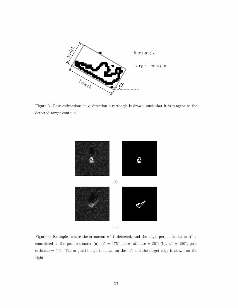
αlength
w
i
d
t
h
Target contour
Rectangle
Figure 3: Pose estimation: in α direction a rectangle is drawn, such that it is tangent to the
detected target contour.
(a)
(b)
Figure 4: Examples where the erroneous α∗ is detected, and the angle perpendicular to α∗ is
considered as the pose estimate: (a), α∗ = 175◦, pose estimate = 85◦; (b), α∗ = 150◦, pose
estimate = 60◦. The original image is shown on the left and the target edge is shown on the
right.
23

(a) (b) (c)
Figure 5: Examples of the vehicles rotated to 180◦: (a) T72, (b) BMP2, and (c) BTR70.
Training set Testing set
serial number size serial number size
BTR70 sn-c71 233 sn-c71 196
sn-9563 233 sn-9563 195
BMP2 sn-9566 232 sn-9566 196
sn-c21 233 sn-c21 196
sn-132 232 sn-132 196
T72 sn-812 231 sn-812 195
sn-s7 228 sn-s7 191
Table 1: Summary of the MSTAR database.
24

AdaBoost
Initialization: D = {(xn, yn)}Nn=1, maximum iteration number T , d(1)(n) = 1/N
for t = 1 : T
1. Train base learner with respect to distribution d(t) and get hypothesis ht(x) : x →[−1, +1].
2. Calculate the edge rt of ht:
rt =
N∑
n=1
d(t)(n)ynht(xn) , (15)
3. Compute the combination coefficient:
αt =1
2ln(1 + rt
1 − rt
)
, (16)
4. Update distributions:
d(t+1)(n) = d(t)(n) exp(−αtynht(xn))/Zt , (17)
where Zt is the normalization constant such that∑N
n=1 d(t+1)(n) = 1, that is,
Zt =N∑
n=1
d(t)(n) exp(−αtynht(xn)) . (18)
end
Output: F (x) =∑T
t=1 αtht(x) .
Figure 6: The pseudo-code of the confidence-rated AdaBoost.
Hamming decoding max correlation decoding
one-against-all 98.68% 99.19%
all-pair 99.05% 99.63%
Table 2: Correct classification rates using both feature sets for S1 setting.
25

Data fusion using AdaBoost
Initialization: D = {((xfn,xr
n), yn)}Nn=1, T , d(1)(n) = 1/N
for t = 1 : T
1a. Train ht on {xfn} with respect to
d(t).
1b. Train ht on {xrn} with respect to
d(t).
2a. Calculate αt as in (16) using the
results from 1a.
2b. Calculate αt as in (16) using the
results from 1b.
3a. Calculate Zt as in (18) using the
results from 1a. and 2a.
3b. Calculate Zt as in (18) using the
results from 1b. and 2b.
3. Choose the branch that gives smaller Zt, and update d(t+1), as in (17), using
ht, αt, and Zt from the selected branch.
end
Output: F (x) =∑T
t=1 αtht(x).
Figure 7: The pseudo-code of AdaBoost as a fusion method.
1 5 10 15 20 25 30 35 40 45 500
0.005
0.01
0.015
0.02
0.025
0.03
number of iteration
clas
sifi
cati
on
err
or
Training errorTesting error
(a)
1 10 20 30 40 500
0.005
0.01
0.015
0.02
0.025
number of iteration
clas
sifi
cati
on
err
or
Training errorTesting error
(b)
Figure 8: Classification error curves of (a) the one-against-others approach, and (b) the all-pair
approach. Both use the max correlation decoding rule. The classifiers are learned by AdaBoost
on all training datasets and tested on all testing datasets.
26

BTR70 BMP2 T72
BTR70 195 1 0
BMP2 0 584 3
T72 0 1 581
Table 3: Confusion matrix of the all-pair encoding and the max correlation decoding rules using
both feature sets for S1 setting.
Hamming decoding max correlation decoding
one-against-all 94.58% 97.36%
all-pair 97.44% 97.80%
Table 4: Correct classification rates of the RBF base learner using both feature sets for S1
setting.
fine features raw features both features
one-against-all 97.07% 97.95% 99.19%
all-pair 97.44% 98.10% 99.63%
Table 5: Correct classification rates for different feature sets using the max correlation decoding
for S1 setting.
Matched Filter MACH Filter neural network AdaBoost
[25] [26] [5] raw features both features
Pcc 98.97% 98.10% 93% 98.10% 99.63%
Table 6: Correct classification rate of different ATR systems for S1 setting. Pcc - probability of
correct classification.
Hamming decoding max correlation decoding
one-against-all 92.45% 95.53%
all-pair 95.46% 96.12%
Table 7: Correct classification rates using both feature sets for S2 setting.
27

BTR70 BMP2 T72
BTR70 192 3 1
BMP2 4 554 29
T72 0 12 570
Table 8: Confusion matrix of the all-pair encoding and the max correlation decoding rules using
both feature sets for S2 setting.
fine features raw features both features
one-against-all 94.65% 92.45% 95.53%
all-pair 95.31% 92.82% 96.12%
Table 9: Correct classification rates for different feature sets using the max correlation decoding
for S2 setting.
Template Matcher [7] neural network [7] SVM [7] AdaBoost
Pcc 89.7% 94.07% 94.87% 96.12%
Pd 90% 90% 90% 100%
Table 10: Correct classification rate of different ATR systems for S2 setting; Pcc - probability
of correct classification, Pd - probability of detection. Note that the classification rate of our
AdaBoost ATR system is calculated for a much higher (100% vs. 90%) detection probability
than for the other systems.
28