Embed Size (px)
Citation preview
Journal of Theoretical and Applied Information Technology 15
th September 2016. Vol.91. No.1
© 2005 - 2016 JATIT & LLS. All rights reserved.
ISSN: 1992-8645 www.jatit.org E-ISSN: 1817-3195
158
ADAPTIVE BACKSTEPPING CONTROL FOR WIND
TURBINES WITH DOUBLY-FED INDUCTION GENERATOR
UNDER UNKNOWN PARAMETERS
1MOHAMMED RACHIDI,
2BADR BOUOULID IDRISSI
1,2Department of Electromechanical Engineering, Moulay Ismaïl University, Ecole Nationale Supérieure
d’Arts et Métiers, BP 4024, Marjane II, Beni Hamed, 50000, Meknès, Morocco
E-mail: [email protected],
ABSTRACT
This paper deals with an adaptive, nonlinear controller for wind systems connected to a stable electrical
grid and using a doubly-fed induction machine as a generator. The study focuses on the case wherein the
aerodynamic torque model and winding resistances of the generator are unknown and will be updating in
real time. Two objectives were fixed; the first one is speed control, which allows us to force the system to
track the optimal torque-speed characteristic of the wind turbine to extract the maximum power, and the
second deals with the control of the reactive power transmitted to the electrical grid. The mathematical
development, both for the model of the global system and the control and update laws, is examined in
detail. The control design is investigated using a backstepping technique, and the overall stability of the
system is shown by employing the Lyapunov theory. The results of the simulation, which was built on
Matlab-Simulink, confirm when compared with control without adaptation, the validity of this work and
the robustness of our control in the presence of parametric fluctuations or uncertainty modeling.
Keywords: Wind power generation, doubly-fed induction generator, unknown winding resistances,
unknown aerodynamic torque, adaptive control, backstepping control, Lyapunov theory.
1. INTRODUCTION
From all sources of electricity generation, that
which has the wind as origin has presented the
highest growth rate for more than 20 years, and this
should continue in the future [1]. Thus, wind
generation should be the greatest contribution to
reducing the greenhouse effect in the coming years.
The causes for this increase lie in the high political
will to promote this sector and also in production
costs, which are becoming increasingly
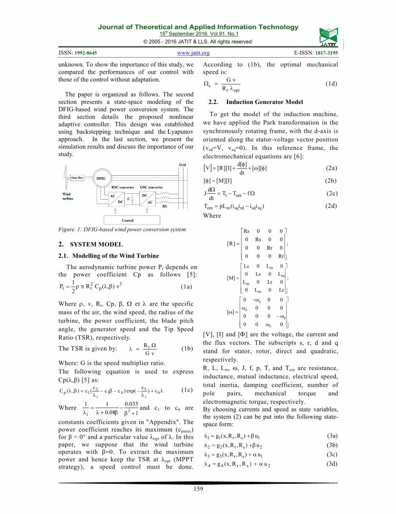
competitive. The most used structure in this area,
especially in high power, which is also the subject
of this work, is shown in Figure 1[2-3]. It uses a
doubly fed induction machine as a generator. In
general, the stator is directly connected to the
electrical grid, but the rotor is connected through
two back-to-back power converts and an RL filter.
The capacitor C is considered as a DC regulated
voltage source for the converts. The rotor side
converter (RSC) is usually used to control the
active and reactive power transmitted from the
stator to grid. However, the grid side converter
(GSC) is used to regulate the DC voltage at a fixed
value and, at the same time, control the reactive
power transmitted the from the RL filter to the grid.
The principal benefit of this configuration is the
possibility of varying the rotor speed in a large
range around the synchronous speed of about ±30%
[2-4]. This allows us to design a speed control that
forces the system to continuously track the optimal
torque-speed characteristic of the wind turbine [11-
12].
The purpose of this work is to take part of this
research area by examining the subject of the
robustness of the control in case of parametric and
modeling uncertainties. Indeed, we have targeted
the pertinent parameters that are susceptible to vary
with the temperature, such as the resistance of the
rotor and stator windings. We also investigated the
case of the aerodynamic torque, for which accurate
modeling is not an easy task. We designed adaptive
controllers that allow us to reach the fixed
performances and, at the same time, to update the
previous parameters that are assumed to be
Journal of Theoretical and Applied Information Technology 15
th September 2016. Vol.91. No.1
© 2005 - 2016 JATIT & LLS. All rights reserved.
ISSN: 1992-8645 www.jatit.org E-ISSN: 1817-3195
159
unknown. To show the importance of this study, we
compared the performances of our control with
those of the control without adaptation.
The paper is organized as follows. The second
section presents a state-space modeling of the
DFIG-based wind power conversion system. The
third section details the proposed nonlinear
adaptive controller. This design was established
using backstepping technique and the Lyapunov
approach. In the last section, we present the
simulation results and discuss the importance of our
study.
Figure. 1: DFIG-based wind power conversion system
2. SYSTEM MODEL
2.1. Modelling of the Wind Turbine
The aerodynamic turbine power Pt depends on
the power coefficient Cp as follows [5]:
3p
2tt v),(CR
2
1P βλπρ=
(1a)
Where ρ, v, Rt, Cp, β, Ω et λ are the specific
mass of the air, the wind speed, the radius of the
turbine, the power coefficient, the blade pitch
angle, the generator speed and the Tip Speed
Ratio (TSR), respectively.
The TSR is given by: vG
R t Ω=λ (1b)
Where: G is the speed multiplier ratio.
The following equation is used to express
Cp(λ,β) [5] as:
λ+λ
−−β−λ
=βλ 6i
543
i
21p c)
cexp()cc
c(c),(C
(1c)
Where 1
035.0
08.0
113
i +β−
β+λ=
λand c1 to c6 are
constants coefficients given in "Appendix". The
power coefficient reaches its maximum (cpmax)
for β = 0° and a particular value λopt of λ. In this
paper, we suppose that the wind turbine
operates with β=0. To extract the maximum
power and hence keep the TSR at λopt (MPPT
strategy), a speed control must be done.
According to (1b), the optimal mechanical
speed is:
opttc
R
vG
λ=Ω (1d)
2.2. Induction Generator Model
To get the model of the induction machine,
we have applied the Park transformation in the
synchronously rotating frame, with the d-axis is
oriented along the stator-voltage vector position
(vsd=V, vsq=0). In this reference frame, the
electromechanical equations are [6]:
[ ] ]][[dt
][d]I][R[V φω+
φ+=
(2a)
]I][M[][ =φ
(2b)
Ω−−=Ω
fTTdt
dJ emt
(2c)
)iiii(pLT rqsdrdsqmem −=
(2d)
Where
;
Rr000
0Rr00
00Rs0
000Rs
]R[
=
;
Lr0L0
0Lr0L
L0Ls0
0L0Ls
]M[
m
m
m
m
=
ω
ω−
ω
ω−
=ω
000
000
000
000
][
r
r
s
s
[V], [I] and [Φ] are the voltage, the current and
the flux vectors. The subscripts s, r, d and q
stand for stator, rotor, direct and quadratic,
respectively.
R, L, Lm, ω, J, f, p, Tt and Tem are resistance,
inductance, mutual inductance, electrical speed,
total inertia, damping coefficient, number of
pole pairs, mechanical torque and
electromagnetic torque, respectively.
By choosing currents and speed as state variables,
the system (2) can be put into the following state-
space form:
1sr11 u)R,R,x(gx β+=&
(3a)
2sr22 u)R,R,x(gx β+=&
(3b)
1sr33 u)R,R,x(gx α+=&
(3c)
2sr44 u)R,R,x(gx α+=&
(3d)
Journal of Theoretical and Applied Information Technology 15
th September 2016. Vol.91. No.1
© 2005 - 2016 JATIT & LLS. All rights reserved.
ISSN: 1992-8645 www.jatit.org E-ISSN: 1817-3195
160
emtF Γ+Γ+η−=η&
(3e)
Where:
Ω=η== ,)i,i,i,i()x,x,x,x(x trqrdsqsd
t4321
J
T);xxxx(a
J
tt3241
emem =Γ−=
Τ−=Γ
rq2rd1 vu,vu ==
sr
m
r LL
L,
L
1
σ−=β
σ=α
The functions )R,R,x(g sri are:
η+η+−−=
β+η−η−+−=
η−η−+−−=
α+η+η+++−=
3x3m1x3n4xrR3a3x3b2xsR3c4g
u4x3m2x3n4x3b3xrR3a1xsR3c3g
3x1n1x1m4xrR1c2xsR1a1x1b2g
u4x1n2x1m3xrR1c2x1b1xsR1a1g
J
fF;
LL
L1;V
,L
Lpn,
pm,
LL
Lc,f2b,
L
1a
,VL
1,
L
Lpn,
1pm
,LL
Lc,f2b,
L
1a,
J
pLa
rs
2m
u
r
m33
rs
m3r3
r3
su
s
m11
rs
m1rs1
s1
m
=−=σβ=β
σ=
σ=
σ=π=
σ=
σ=α
σ=
σ
σ−=
σ=π=ω=
σ==
fr and V are respectively the constant frequency and
magnitude of grid voltage.
Equations (3a) to (3.d) can be put into the following
compact form:
uA)R,R,x(gx sr +=&
(3f)
Where
,)g,g,g,g(g t4321= t
21 )u,u(u = ,
t
00
00A
αβ
αβ=
3. CONTROL DESIGN
3.1. Control objectives
By examining the equation system (3), we can
identify two degrees of freedom u1 and u2 that can
be used to control the RSC converter. Thus, two
control objectives were set; the first one is speed
control, which allows us to force the system
to extract the maximum power, while the second
deals with the control of reactive power transmitted
by the stator to the electrical grid. To achieve this
goal, we used the Backstepping technique [7-8].
Indeed, the following expression of the stator
reactive power
2sqsdsdsqsg xViviv)IVIm(Q −=−== ∗
(4)
shows that the current variable x2 can be used to
control the reactive power Qsg. According to
equation (3b), it is clear that the control variable u2
can be designed so that the current variable x2
tracks its reference. On the other hand, from the
system (3), we can reconstruct the following
subsystem that adapts well to control speed:
β−α+α−β+∇=Γ
Γ+Γ+η−=η
231124em
emt
u)xx(au)xx(ag.h
F
&
&
(5)
Where
)xxxx(a)x(h 3241em −=Γ=
and )x
h,
x
h,
x
h,
x
h(h
4321 ∂
∂
∂
∂
∂
∂
∂
∂=∇
So, in the first equation, the variable Γem can be
considered as a virtual control for the speed η. The
second equation shows that the control variable u1
can be designed so that Γem tracks its reference.
3.1.2. Control and update laws
For uncertain model to which the parameters are
not known with sufficient accuracy, an appropriate
choice of control and update laws must be done to
still ensure the stability condition. In this study, it is
assumed that the stator resistance, rotor resistance
and mechanical torque Rs, Rr and Tt, respectively,
are unknown and vary slowly with time. Their
corresponding estimated terms are denoted rs R,R
and tΓ , respectively. We define also the error
variables as:
ttt
sss
rrr
emcem2
c1
c220
ˆ~RRR
~RRR
~z
z
xxz
Γ−Γ=Γ
−=
−=
Γ−Γ=
η−η=
−=
(6)
Where cc2 ,x η and emcΓ are the references of
variables x2, η and Γem, respectively.
Proposition: The following update and control
laws:
Journal of Theoretical and Applied Information Technology 15
th September 2016. Vol.91. No.1
© 2005 - 2016 JATIT & LLS. All rights reserved.
ISSN: 1992-8645 www.jatit.org E-ISSN: 1817-3195
161
)z)x(hzx(aR
)z)x(hazxc(R
ˆ
v)F()x(h
2021ss
23041rr
ttt
tttttt
+γ−=
−γ=
ηλ+ξ=Γ
−ηλ−λ+λ−ξλ−=ξ
&
&
&
)xx(a
u)xx(ag.hˆu
;xzk)R,R,x(g
u
24
2311
c200sr22
α−β
β−α−∇−υ=
β
+−−=
&
With
constantsdesign positivesare,,k,k,k
))R,R,x(gx)R,R,x(gx
)R,R,x(gx)R,R,x(gx(ag.h
v)zzk)(Fk(Fzkzˆ
z)Fk(zv
)xxxx(a)x(h
ˆFz)Fk(
tr210
sr23sr32
sr14sr41
tC2111c221
21t1t
3241em
Ctc11emc
λγ
−−
+=∇
+η++−+η+−=υ
−+λ−−=
−==Γ
η+Γ−η+−−=Γ
&&&
&
achieve speed and current tracking objectives and
ensure asymptotic stability despite the changes in
parameters.
Proof:
a- Control law 2u
Taking the derivative of z0 and using (3b), we can
write:
c22sr20 xu)R,R,x(gz && −β+=
(7)
With the Lyapunov candidate function 200 z
2
1V =
and the choice 000 zkz −=& , where k0 is a positive
design constant, it’s possible to make negative the
derivative 0zkV2000 ≤−=& .
The control law u2 can be obtained from equation
(7), using the previous choice and the estimated
resistances, as:
β
+−−= c200sr2
2
xzk)R,R,x(gu
&
(8)
So, the dynamic of the error z0 is governed by:
2s14r1000 xR~
axR~
czkz −+−=& (9)
This can be obtained from (7) by using (8) and
noting that
4r12s1sr2sr2 xR~
cxR~
a)R,R,x(g)R,R,x(g +−= .
b- Control u1 and update laws
Step 1: Virtual control emcΓ
Using equation (3e), the derivative of z1 is written
as:
Cemt1 Fz η−Γ+Γ+η−= &&
(10)
Since tΓ is unknown; it will be replaced with its
estimated tΓ . With the Lyapunov candidate function
211 z
2
1V = and the choice 111 zkz −=& , where k1 is a
positive design constant, it’s possible to make
negative the derivative 0zkV2111 ≤−=& .
Using this choice, equation (10) becomes:
Cemct11ˆFzk η−Γ+Γ+η−=− &
(11)
Thus, the virtual control emcΓ is:
Ctc11emcˆFz)Fk( η+Γ−η+−−=Γ &
(12)
Where η has been replaced by
c1z η+
Subtracting (11) from (10), we obtain:
t2111~
zzkz Γ+−−=&
(13)
Step 2: Control and update laws
We will now proceed in the same way for the
derivative 2z& .
emcem2z Γ−Γ= &&& (14)
Firstly, we express emΓ& according to (5):
Using (6), the detailed development of the term
g.h∇ gives:
)x(hR~
a)x(hR~
ag.hg.h s1r3 −−∇=∇
Where
))R,R,x(gx)R,R,x(gx
)R,R,x(gx)R,R,x(gx(ag.h
sr23sr32
sr14sr41
−−
+=∇
To separate unknown terms from the rest, we write
emΓ& as:
)x(hR~
a)x(hR~
aˆ s1r3em −−υ=Γ&
Where
231124 u)xx(au)xx(ag.hˆ β−α+α−β+∇=υ (15)
Secondly, taking the derivative of emcΓ from (12)
and using (13), we can write emcΓ& as:
Journal of Theoretical and Applied Information Technology 15
th September 2016. Vol.91. No.1
© 2005 - 2016 JATIT & LLS. All rights reserved.
ISSN: 1992-8645 www.jatit.org E-ISSN: 1817-3195
162
Ctct2111emcˆF)
~zzk)(Fk( η+Γ−η+Γ+−−−−=Γ &&
&&&
Thus the dynamic of error 2z is:
Ctct2
111s1r32
ˆF)~
z
zk)(Fk()x(hR~
a)x(hR~
aˆz
η−Γ+η−Γ+−
−−+−−υ=
&&&
&
&
(16)
To update the torque, one proposes the dynamic of
error estimation t
~Γ as [9]:
tttt v~~
+Γλ−=Γ&
(17)
Where tλ is a positive design constant and tv is a
term to be determined after.
If we combine (17) and the equation of motion (3e),
we can establish the update law of the torque as:
ttttttttt v)F()x(h)ˆ(ˆ −ηλ−λ+λ−ηλ−Γλ−=ηλ−Γ &&
For this law, we have assumed that the torque
varies slowly, which results in: ttˆ~Γ−=Γ&&
By using ηλ−Γ=ξ tttˆ as intermediate variable,
one can rewrite the update law of the torque as:
ηλ+ξ=Γ
−ηλ−λ+λ−ξλ−=ξ
ttt
tttttt
ˆ
v)F()x(h&
(18)
Equation (16) can be now put in the form:
t1ts1r32
~)Fk()x(hR
~a)x(hR
~aAz Γ−+λ+−−=& (19)
Where
tC2111c v)zzk)(Fk(FˆA −η−−−−+η−υ= &&& (20)
To ensure the overall stability, one proposes the
following Lyapunov candidate function:
2
~
R~
2
1R~
2
1z
2
1z
2
1z
2
1V
2t2
ss
2r
r
22
21
20
Γ+
γ+
γ+++= (21)
Using (9), (13) and (19), V& can be written as
follows:
sss
21021
tt21t1rrr
230412
tt21211
200
R~
)R1
z)x(hazxa(
~)vz)Fk(z(R
~)R
1
z)x(hazxc(~
z)zA(zkzkV
&
&
&
γ−−−+
Γ+−+λ++γ
−
−+Γλ−−+−−=
The update laws are obtained by cancelling the
terms with rR~
and t
~Γ :
21t1t z)Fk(zv −+λ−−=
)z)x(hazxc(R 23041rr −γ=&
)z)x(hzx(aR 2021ss +γ−=&
By choosing 221 zkzA −= , equation (19) becomes:
t1ts1r32212~
)Fk()x(hR~
a)x(hR~
azkzz Γ−+λ−−−−=& (22)
And the derivative V& reduces to:
0~
zkzkzkV2
tt222
211
200 ≤Γλ−−−−=&
Which implies that the errors 0z , 1z , 2z and t
~Γ
converge to zero.
Equations (9) and (22) show that if h(x) is different
from zero then, errors rR~
and sR~
converge also to
zero.
Finally, by using (15) one can establish the control
law u1 as:
)xx(a
u)xx(ag.hˆu
24
2311 α−β
β−α−∇−υ=
For this expression, the term υ is determined, by
replacing the term A in the equation (20) by
221 zkz − , as:
tC2111c221 v)zzk)(Fk(Fzkzˆ +η++−+η+−=υ &&&
Remark:
sqrr
rqrr
msq
r24
LL
a)i
LL
Li
L
1(a)xx(a φ
σ−=
σ−
σ−=α−β
Since the effect of the stator resistance is
negligible especially in high power, the flux and
the voltage vectors are substantially orthogonal.
Then, with the frame used for the induction
machine, the term sqφ is equal to the amplitude
of the stator flux. Consequently, the term
)xx(a 24 α−β becomes different from zero as
soon as the system is connected to the grid.
4. SIMULATION RESULTS
The simulation built on Matlab / Simulink deals
with the entire wind system shown in Figure 1. In a
previous paper [10], we developed the GSC
converter control and for which we are interested
for regulating the DC voltage and reactive power
transmitted from the rotor to the grid. This power is
proportional to the quadratic component of the
phase current, noted i0q, passing through the filter
RL (see Eq(4)). To show the importance of this
paper, we developed two simulation schemes,
which corresponded respectively to the
conventional (with known model) and our adaptive
Journal of Theoretical and Applied Information Technology 15
th September 2016. Vol.91. No.1
© 2005 - 2016 JATIT & LLS. All rights reserved.
ISSN: 1992-8645 www.jatit.org E-ISSN: 1817-3195
163
(with unknown resistances and mechanical torque
model) backstepping controllers.
The tracking and identifying capability of our
adaptive controller were verified in the case of
time-varying wind speed (Figures 3). To
demonstrate the robustness against winding
resistances and mechanical torque changes,
regulation performances for adaptive and
conventional controllers were compared at constant
wind speed (Figures 4). For both cases, one
assumes that changes occur in the system model,
first (at 10s, ∆Rr=50%) and next in the mechanical
torque (at 20s, ∆Tt=-50%).
The constant values for DC-link voltage filter and
quadratic currents references were considered. To
have a unity power factor, the references of q-axis
currents isq and ioq have been set to zero. The values
of the design parameters used in simulation are:
k0 =1000, k1 =150, k2 =2000, λt=10 and
γs=γr =0.0001.
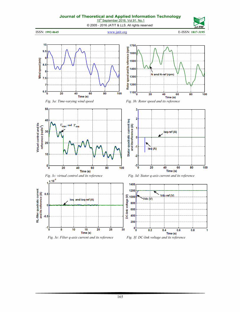
Figures 3a and 3b confirm the effectiveness of
the MPPT strategy since the rotor speed varies in
accordance with wind speed so that the turbine
operates at its optimal TSR.
Figures 3d and 3e show the good tracking
capability of the q-axis current controller. The same
performances are achieved in the case of DC-link
regulation (Figure 3f) and the virtual control
variable (Figure 3c).
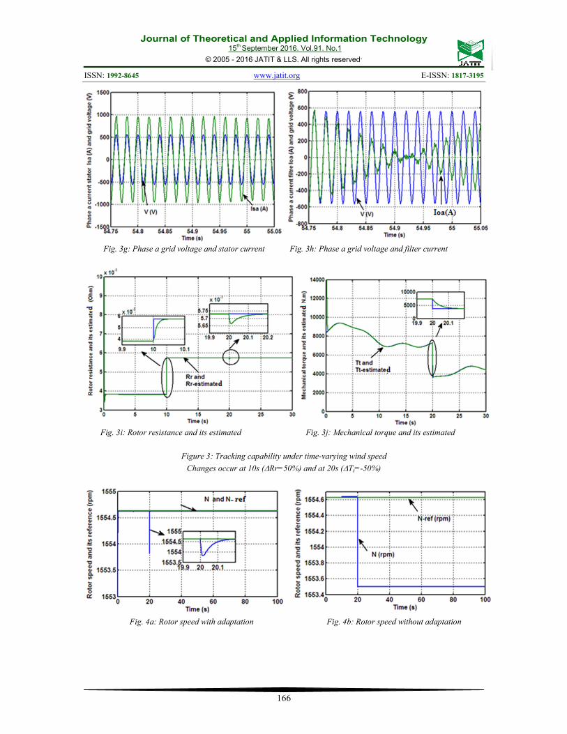
Figures 3g and 3h illustrate the two operating
modes of the generator. Around time t=55s, we can
see in Figure 3b that the induction machine
switches from super-synchronous to sub-
synchronous mode (Ns=1500 rpm). Figure 3g
shows that grid voltage and stator current are in
phase for both of the two operating modes; thus, the
active power is transmitted from the stator to the
grid. Figure 3h shows that grid voltage and filter
current are in phase opposition for (t>55s); thus, the
active power is transmitted from the grid to the
rotor. This result is compatible with the sub-
synchronous speed operation. Also, Figure
(3h) shows that, for (t<55s), the grid voltage and
filter current are in phase; thus, the active power is
transmitted from the grid to the rotor. This result is
compatible with the super-synchronous speed
operation.
According to Figure 3i, one can notice that the
unknown rotor resistance quickly converges to its
true profile (unknown to the controller). Likewise,
Figure 3j shows that the estimated mechanical
torque recovers perfectly the applied unknown
aerodynamic torque.
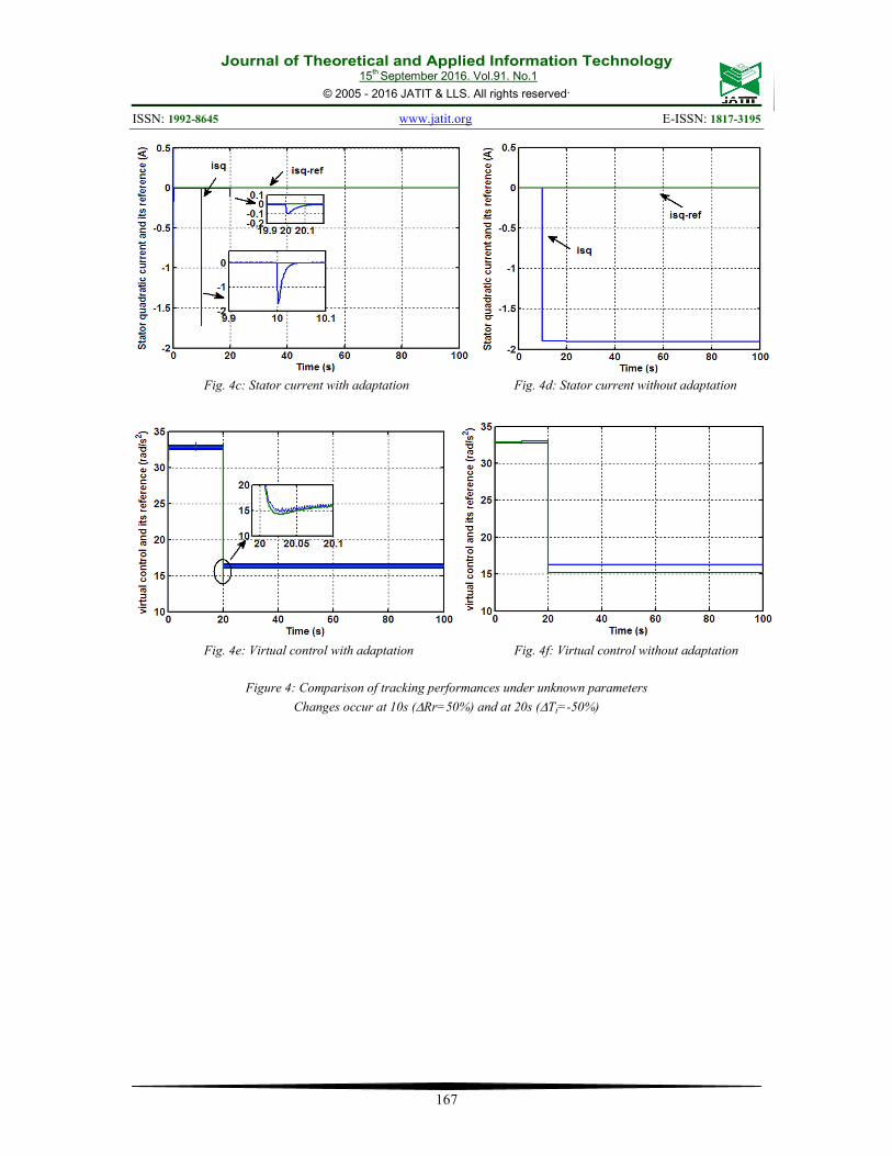
Figure 4 shows the regulation performances of
the conventional and adaptive controllers
when there are changes in the rotor resistance Rr
and the mechanical torque Tt. The simulation
assumes that changes occur in the system model
first at 10s, ∆Rr=50% and next in the mechanical
torque at 20s, ∆Tt=-50%. Unlike the conventional
backstepping controller (Figures. 4b, 4d, and 4f),
the adaptive controller tracks correctly the
references of regulated variables despite the
changes (Figures. 4a, 4c, and 4e). These results
confirm the robustness of the proposed controller.
5. CONCLUSION
This paper has shown the effectiveness and
robustness of a nonlinear, adaptive, backstepping
controller in variable-speed DFIG systems with
unknown aerodynamic torque models and unknown
resistances of rotor and stator winding. The
numerical simulation shows the good speed, current
tracking performances, and the correct update and
identification of unknown parameters. Finally, the
comparison with the conventional controller
without adaptations shows the superiority of the
proposed adaptive controller and the pertinence of
this work.
Journal of Theoretical and Applied Information Technology 15
th September 2016. Vol.91. No.1
© 2005 - 2016 JATIT & LLS. All rights reserved.
ISSN: 1992-8645 www.jatit.org E-ISSN: 1817-3195
164
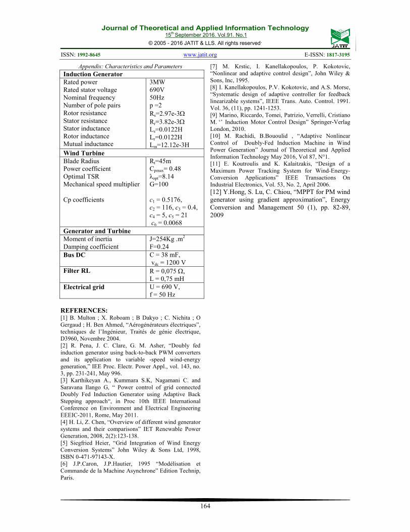
Appendix: Characteristics and Parameters
Induction Generator
Rated power
Rated stator voltage
Nominal frequency
Number of pole pairs
Rotor resistance
Stator resistance
Stator inductance
Rotor inductance
Mutual inductance
3MW
690V
50Hz
p =2
Rs=2.97e-3Ω
Rr=3.82e-3Ω
Ls=0.0122H
Lr=0.0122H
Lm=12.12e-3H
Wind Turbine
Blade Radius
Power coefficient
Optimal TSR
Mechanical speed multiplier
Cp coefficients
Rt=45m
Cpmax= 0.48
λopt=8.14
G=100
c1 = 0.5176,
c2 = 116, c3 = 0.4,
c4 = 5, c5 = 21
c6 = 0.0068
Generator and Turbine
Moment of inertia
Damping coefficient
J=254Kg .m2
F=0.24
Bus DC C = 38 mF,
vdc = 1200 V
Filter RL R = 0,075 Ω,
L = 0,75 mH
Electrical grid U = 690 V,
f = 50 Hz
REFERENCES: [1] B. Multon ; X. Roboam ; B Dakyo ; C. Nichita ; O
Gergaud ; H. Ben Ahmed, “Aérogénérateurs électriques”,
techniques de l’Ingénieur, Traités de génie électrique,
D3960, Novembre 2004.
[2] R. Pena, J. C. Clare, G. M. Asher, “Doubly fed
induction generator using back-to-back PWM converters
and its application to variable -speed wind-energy
generation,” IEE Proc. Electr. Power Appl., vol. 143, no.
3, pp. 231-241, May 996.
[3] Karthikeyan A., Kummara S.K, Nagamani C. and
Saravana Ilango G, “ Power control of grid connected
Doubly Fed Induction Generator using Adaptive Back
Stepping approach“, in Proc 10th IEEE International
Conference on Environment and Electrical Engineering
EEEIC-2011, Rome, May 2011.
[4] H. Li, Z. Chen, “Overview of different wind generator
systems and their comparisons” IET Renewable Power
Generation, 2008, 2(2):123-138.
[5] Siegfried Heier, “Grid Integration of Wind Energy
Conversion Systems” John Wiley & Sons Ltd, 1998,
ISBN 0-471-97143-X.
[6] J.P.Caron, J.P.Hautier, 1995 “Modélisation et
Commande de la Machine Asynchrone” Edition Technip,
Paris.
[7] M. Krstic, I. Kanellakopoulos, P. Kokotovic,
“Nonlinear and adaptive control design”, John Wiley &
Sons, Inc, 1995.
[8] I. Kanellakopoulos, P.V. Kokotovic, and A.S. Morse,
“Systematic design of adaptive controller for feedback
linearizable systems”, IEEE Trans. Auto. Control. 1991.
Vol. 36, (11), pp. 1241-1253.
[9] Marino, Riccardo, Tomei, Patrizio, Verrelli, Cristiano
M. ‘’ Induction Motor Control Design” Springer-Verlag
London, 2010.
[10] M. Rachidi, B.Bououlid , “Adaptive Nonlinear
Control of Doubly-Fed Induction Machine in Wind
Power Generation” Journal of Theoretical and Applied
Information Technology May 2016, Vol 87, N°1.
[11] E. Koutroulis and K. Kalaitzakis, “Design of a
Maximum Power Tracking System for Wind-Energy-
Conversion Applications” IEEE Transactions On
Industrial Electronics, Vol. 53, No. 2, April 2006.
[12] Y.Hong, S. Lu, C. Chiou, “MPPT for PM wind
generator using gradient approximation”, Energy
Conversion and Management 50 (1), pp. 82-89,
2009
Journal of Theoretical and Applied Information Technology 15
th September 2016. Vol.91. No.1
© 2005 - 2016 JATIT & LLS. All rights reserved.
ISSN: 1992-8645 www.jatit.org E-ISSN: 1817-3195
165
Fig. 3a: Time-varying wind speed Fig. 3b: Rotor speed and its reference
Fig. 3c: virtual control and its reference Fig. 3d: Stator q-axis current and its reference
Fig. 3e: Filter q-axis current and its reference Fig. 3f: DC-link voltage and its reference
Journal of Theoretical and Applied Information Technology 15
th September 2016. Vol.91. No.1
© 2005 - 2016 JATIT & LLS. All rights reserved.
ISSN: 1992-8645 www.jatit.org E-ISSN: 1817-3195
166
Fig. 3g: Phase a grid voltage and stator current Fig. 3h: Phase a grid voltage and filter current
Fig. 3i: Rotor resistance and its estimated Fig. 3j: Mechanical torque and its estimated
Figure 3: Tracking capability under time-varying wind speed
Changes occur at 10s (∆Rr=50%) and at 20s (∆Tt=-50%)
Fig. 4a: Rotor speed with adaptation Fig. 4b: Rotor speed without adaptation
Journal of Theoretical and Applied Information Technology 15
th September 2016. Vol.91. No.1
© 2005 - 2016 JATIT & LLS. All rights reserved.
ISSN: 1992-8645 www.jatit.org E-ISSN: 1817-3195
167
Fig. 4c: Stator current with adaptation Fig. 4d: Stator current without adaptation
Fig. 4e: Virtual control with adaptation Fig. 4f: Virtual control without adaptation
Figure 4: Comparison of tracking performances under unknown parameters
Changes occur at 10s (∆Rr=50%) and at 20s (∆Tt=-50%)