Embed Size (px)
Citation preview

Adaptive Algorithms for Problems Involving
Black-Box Lipschitz Functions
by
Ilya Baran
B.S., Massachusetts Institute of Technology (2003)
Submitted to the Department of Electrical Engineering and ComputerScience
in partial fulfillment of the requirements for the degree of
Master of Engineering
at the
MASSACHUSETTS INSTITUTE OF TECHNOLOGY
June 2004
c© Massachusetts Institute of Technology 2004. All rights reserved.
Author . . . . . . . . . . . . . . . . . . . . . . . . . . . . . . . . . . . . . . . . . . . . . . . . . . . . . . . . . . . . . .Department of Electrical Engineering and Computer Science
May 20, 2004
Certified by. . . . . . . . . . . . . . . . . . . . . . . . . . . . . . . . . . . . . . . . . . . . . . . . . . . . . . . . . .Erik D. Demaine
Assistant Professor
Thesis Supervisor
Accepted by . . . . . . . . . . . . . . . . . . . . . . . . . . . . . . . . . . . . . . . . . . . . . . . . . . . . . . . . .
Arthur C. SmithChairman, Department Committee on Graduate Students

2
Adaptive Algorithms for Problems Involving
Black-Box Lipschitz Functions
by
Ilya Baran
Submitted to the Department of Electrical Engineering and Computer Scienceon May 20, 2004, in partial fulfillment of the
requirements for the degree ofMaster of Engineering
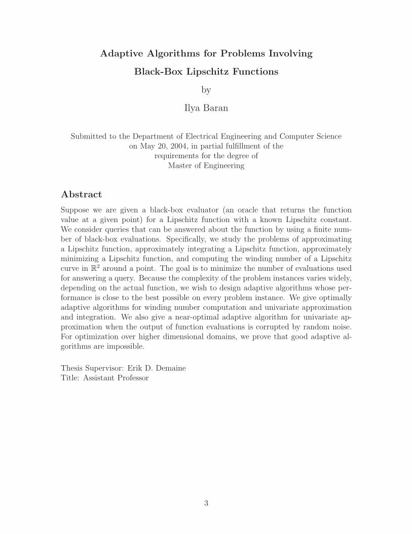
Abstract
Suppose we are given a black-box evaluator (an oracle that returns the functionvalue at a given point) for a Lipschitz function with a known Lipschitz constant.We consider queries that can be answered about the function by using a finite num-ber of black-box evaluations. Specifically, we study the problems of approximatinga Lipschitz function, approximately integrating a Lipschitz function, approximatelyminimizing a Lipschitz function, and computing the winding number of a Lipschitzcurve in R
2 around a point. The goal is to minimize the number of evaluations usedfor answering a query. Because the complexity of the problem instances varies widely,depending on the actual function, we wish to design adaptive algorithms whose per-formance is close to the best possible on every problem instance. We give optimallyadaptive algorithms for winding number computation and univariate approximationand integration. We also give a near-optimal adaptive algorithm for univariate ap-proximation when the output of function evaluations is corrupted by random noise.For optimization over higher dimensional domains, we prove that good adaptive al-gorithms are impossible.
Thesis Supervisor: Erik D. DemaineTitle: Assistant Professor
3

Acknowledgements
I would like to thank my advisor, Erik Demaine, for guiding me on this project,
providing crucial ideas and feedback, and often assisting me in the tricky task of
determining the value of various results.
I would also like to thank Dmitriy “Dimdim” Rogozhnikov for many fruitful and
interesting discussions, some of which led to the most important ideas in Chapters 4
and 5.
Finally, thanks to my other friends, who provided a wonderful haven from this
project and to my parents and sister, who, among other things, gave me free access
to their washing machine.
This research was partially supported by the Akamai Presidential Fellowship.
4
Contents
1 Introduction 7
1.1 Adaptive Algorithms . . . . . . . . . . . . . . . . . . . . . . . . . . . 7
1.2 Problems . . . . . . . . . . . . . . . . . . . . . . . . . . . . . . . . . . 9
1.3 Related Work . . . . . . . . . . . . . . . . . . . . . . . . . . . . . . . 10
1.4 Proof Sets . . . . . . . . . . . . . . . . . . . . . . . . . . . . . . . . . 11
2 Functions from R to R 13
2.1 Sampling Univariate Functions . . . . . . . . . . . . . . . . . . . . . . 13
2.2 Approximation . . . . . . . . . . . . . . . . . . . . . . . . . . . . . . 16
2.3 Integration . . . . . . . . . . . . . . . . . . . . . . . . . . . . . . . . . 21
3 Functions from R to Rd 31
3.1 Lipschitz Curves . . . . . . . . . . . . . . . . . . . . . . . . . . . . . 31
3.2 Approximation . . . . . . . . . . . . . . . . . . . . . . . . . . . . . . 32
3.3 Winding Number . . . . . . . . . . . . . . . . . . . . . . . . . . . . . 35
4 Noisy Samples 41
4.1 Noisy Approximation Problem . . . . . . . . . . . . . . . . . . . . . . 41
4.2 Sampling the Normal Distribution . . . . . . . . . . . . . . . . . . . . 43
4.3 Noisy Algorithm . . . . . . . . . . . . . . . . . . . . . . . . . . . . . 48
4.4 Bounds on OPT in Terms of NOPT . . . . . . . . . . . . . . . . . . . 51
5 Functions Whose Domain is in Rd 55
5.1 Higher Dimensional Domains . . . . . . . . . . . . . . . . . . . . . . 55
5

5.2 Lower Bounds for Function Minimization . . . . . . . . . . . . . . . . 56
6 Conclusion 59
6.1 Results Summary . . . . . . . . . . . . . . . . . . . . . . . . . . . . . 59
6.2 Future Research . . . . . . . . . . . . . . . . . . . . . . . . . . . . . . 60
6
Chapter 1
Introduction
1.1 Adaptive Algorithms
Algorithms can be analyzed in many different ways. Worst-case analysis measures
an algorithm’s slowest performance on a problem of size n. Average-case analysis
measures the “average” performance on problems of size n (for a suitably defined
“average”). Competitive analysis compares an online algorithm’s performance on a
problem instance to the best possible output of an algorithm that has access to the
entire problem instance. In this thesis, I focus on adaptive analysis, which compares
the performance of the algorithm to the difficulty of the particular problem instance.
The terms “performance” and “difficulty” are intentionally vague because they can
be defined in various ways.
As an example, consider the problem of sorting in the comparison model (see
[CLRS01] for an overview). Performance for this problem is measured by the number
of comparisons an algorithm performs. A well-known lower bound is that Ω(n log n)
comparisons are necessary in the worst case. Mergesort, for example, performs
O(n log n) comparisons in the worst case, so there is no “better” algorithm than
mergesort (neglecting constant factors) from the worst-case point of view. However,
if most problem instances are already almost sorted, we may wish for an algorithm
that performs better if, for instance, the initial order of the objects has few inversions.
Such an algorithm is known, in fact: it requires O(n+n log(1+ I/n)) comparisons to
7
sort an input that has n objects and I inversions. This is an adaptive algorithm and
it performs better for easier instances. Many other adaptive algorithms for sorting
are known, for different notions of difficulty. See [ECW92] for a survey of them. It
is important to note that an adaptive algorithm does not know the difficulty of the
problem (for instance, the number of inversions) in advance—it discovers how difficult
the problem is as it runs and adapts to this difficulty.
For some problems, particularly the ones I wish to consider, a natural measure
of the difficulty of a problem instance is the performance of the best-possible (cor-
rect) algorithm for that problem instance. More formally, if P is the set of problem
instances, A is the set of algorithms (in some reasonable class) that are correct on
all problem instances, and COST(A, P ) is the cost incurred by algorithm A ∈ A on
problem instance P ∈ P, then the best-possible performance (denoted OPT(P )) is:
OPT(P )def= inf
A∈ACOST(A, P ).
Our terminology regarding OPT is a bit sloppy: we use OPT to refer to both the
performance of the best-possible algorithm and to the best-possible algorithm itself—
from the context, it is always clear which meaning is intended.1
By definition, for each problem instance P , there is an algorithm whose cost on
P is arbitrarily close to OPT(P ). We are interested in adaptive algorithms whose
cost on P is not much greater than OPT(P ) for every problem instance P . Carrying
out an adaptive analysis for an algorithm is generally more difficult than carrying
out a worst-case analysis, because the former makes stronger performance guaran-
tees. If difficult problem instances are rare (as sometimes happens in practice), an
adaptive algorithm performs much better than an algorithm whose performance on
every problem instance is its worst-case performance.
1When possible values of COST are not discrete (as can happen with expected costs), a best-possible algorithm may not exist. Because we ignore constant factors, an algorithm whose cost iswithin an additive constant of the best possible is sufficient for our purposes.
8
1.2 Problems
In this thesis, we study deterministic adaptive algorithms for answering queries about
Lipschitz functions. The Lipschitz condition is a weak condition on a function (it is
slightly stronger than continuity), but it allows interesting algorithms. A typical
problem is a special case of the following:
Let S be a subset of Rd, and let M be a metric space. Let f be a
function from S to M such that for every x1, x2 ∈ S, the Lipschitz con-
dition is satisfied: dM(f(x1), f(x2)) ≤ L‖x2 − x1‖2. Compute a property
of f with error at most ǫ, for ǫ > 0. An algorithm can obtain information
about f only by sampling (evaluating) it at a point of S and should use
as few samples as possible.
Problems with such formulations are also studied in the field of information-based
complexity (see [TWW88] for an overview). However, information-based complexity
is primarily concerned with worst-case, average-case, or randomized analysis of more
difficult problems, rather than adaptive analysis of algorithms for easier problems.
Note that in information-based complexity, the term “adaptive algorithm” refers to
an algorithm in which the locations where f is sampled are allowed to depend on the
results of previous samples of f . However, we use the term “adaptive algorithm” in
the sense of [DLOM00].
This thesis is organized by the type of function for which the problem is posed.
In Chapter 2, we study problems on Lipschitz functions from [0, 1] to R. We consider
the problem of approximating such a function and the problem of approximating its
definite integral. In Chapter 3, we extend the results on the approximation problem
to the setting when the range is an arbitrary metric space. We also give an adaptive
algorithm for computing the winding number of a Lipschitz curve in R2. In Chap-
ter 4, we consider the approximation problem when the values of the samples an
algorithm makes are corrupted by random noise. Finally, in Chapter 5, we consider
the optimization problem when the domain is d-dimensional with d ≥ 2.
9
The final goal of investigating a problem in the adaptive framework is to de-
sign an optimally adaptive algorithm. Suppose P is the set of problem instances
and each problem instance P ∈ P has certain natural parameters, v1(P ), . . . , vk(P ),
with the first parameter v1(P ) = OPT(P ). An algorithm is optimally adaptive if its
performance on every problem instance P ∈ P is within a constant factor of every
algorithm’s worst-case performance on the family of instances P ′ ∈ P | vi(P′) =
vi(P ) for all i. Note that this definition depends on the choice of parameters. In
addition to OPT, we choose reasonable parameters, such as ǫ, the desired output
accuracy. For some problems, it is possible to come up with instance-optimal algo-
rithms. An algorithm is instance optimal if its performance is within a constant factor
of OPT on every problem instance. Obviously, any instance-optimal algorithm is op-
timally adaptive. In this thesis, we give an instance-optimal algorithm for winding
number computation and optimally adaptive algorithms for univariate approximation
and deterministic univariate integration. The results we achieve are summarized in
Table 6.1 in the conclusion.
When discussing the problems, we assume without loss of generality that the
Lipschitz constant is 1. The function and relevant parameters can be scaled to make
this the case. Also, when the domain of the function is an interval, we assume that
this interval is [0, 1], for the same reason.
1.3 Related Work
There is not very much literature on adaptive algorithms that perform well relative
to OPT. One reason is that adaptive analysis makes a much stronger guarantee
than, for example, worst-case or average-case analysis, and can be more difficult to
perform, as a result. Another reason is that adaptive analysis does not yield itself
well to composition. In other words, if algorithm A uses adaptive algorithm B as a
subroutine, in order for the analysis of A to take advantage of B’s adaptiveness, it
must be shown that the problem instances A feeds to B are “easy”.
Adaptive algorithms have been considered in the context of various set opera-
10
tions in [DLOM00], aggregate ranking in [FLN03], and independent-set discovery in
[BBD+04]. They have also appeared in the context of distributed algorithms: for
example, an adaptive algorithm for the distributed minimum spanning tree problem
is given in [Elk04]. There is extensive literature on univariate Lipschitz function op-
timization, primarily concerned with worst-case or experimental analysis (see, e.g.
[HJ95]), but Piyavskii’s algorithm [Piy72] has been analyzed in the adaptive frame-
work, first in [Dan71]. The analysis was completed and sharpened in [HJL91] to show
that Piyavskii’s algorithm is instance-optimal. [BD04] considers the problem of uni-
variate Lipschitz function optimization when the range is Rd and gives an optimally
adaptive algorithm.
Problems on Lipschitz functions similar to ones we consider have been studied
outside the adaptive framework. For example, [ZKS03] describe an algorithm for
function approximation that is essentially lipschitz-integrate-adaptive, our al-
gorithm for integration (this makes sense because they consider approximation error
averaged over [0, 1], whereas we work with worst-case approximation error). However,
in that paper, it is only shown that the algorithm makes locally optimal choices (i.e.,
it is greedy) and no global optimality analysis of the algorithm is performed. The
univariate Lipschitz integration problem is used to illustrate information-based com-
plexity concepts in [Wer02], and the trivial algorithm is shown to be optimal in the
worst case. In [GW90], problems on Lipschitz curves are considered. A data structure
based on Proposition 8 is proposed for solving curve queries, including nearest-point
queries and point containment (a special case of winding number) and algorithms
based on this data structure are analyzed in the worst case.
1.4 Proof Sets
In order to compare the running time of an algorithm on a problem instance to OPT,
we define the concept of a proof set for a problem instance. A set S of points in the
domain of f is a proof set for problem instance (f, C) (where C represents additional
problem instance components) and output x if for every f ′ that is equal to f on S,
11
x is a correct output on (f ′, C). In other words, sampling f at a proof set proves the
correctness of the output. For example, suppose that the problem is to compute the
definite integral of a Lipschitz function f : [0, 1] → R, to an accuracy of ǫ. A proof
set for problem instance (f, ǫ) and output x is a set of points s1, . . . , sn in [0, 1] such
that for any f with f(si) = f(si), the output is correct:∣
∣
∣x−
∫
f∣
∣
∣≤ ǫ. We say that a
set of samples is a proof set for a particular problem instance without specifying the
output if some output exists for which it is a proof set.
It is clear from the definition that sampling a proof set is the only way a deter-
ministic algorithm can guarantee correctness: if an algorithm doesn’t sample a proof
set for some problem instance, we can feed it a problem instance that has the same
value on the sampled points, but for which the output of the algorithm is incorrect.
Conversely an algorithm can terminate as soon as it has sampled a proof set and
always be correct. Thus, deterministic OPT is equal to the size of a smallest proof
set.
In this thesis, we consider only deterministic algorithms (in Chapter 4, noise in
our model can serve as a random number generator for a deterministic algorithm,
so randomization gives no additional power there). However, we remark that several
alternative models can be considered. If randomization is allowed, but an algorithm
is never allowed to fail, randomized OPT is no more powerful than deterministic
OPT on any black-box Lipschitz problem (because if there is a possibility of an
algorithm terminating after sampling a set of samples that is not a proof set, there
is a possibility of failure). If an algorithm is required to be correct with probability
1, there are some contrived problems on which randomized OPT is more powerful
than deterministic OPT. If correctness with probability at least 2/3 is required,
randomized OPT becomes asymptotically more powerful than deterministic OPT for
integration (we plan to explore this in a forthcoming paper), but no power is gained
for univariate approximation and optimization, and winding number.
12
Chapter 2
Functions from R to R
2.1 Sampling Univariate Functions
In general, a deterministic adaptive algorithm works by sampling the input function
until the samples form a proof set for the problem the algorithm is trying to solve.
To analyze such an algorithm, we compare the number of samples it performs to the
size of a smallest proof set for that problem instance. To do this, we fix a proof set
P , classify the samples the algorithm performs based on their relationship to points
in P , and bound the number of points of some of these classes.
Let P be a nonempty finite set of points in [0, 1]. Consider the execution of an
algorithm which samples a function at points on the interval [0, 1) (if it samples at 1,
ignore that sample). Let s1, s2, . . . , sn be the sequence of samples that the algorithm
performs in the order that it performs them. Let It be the set of unsampled intervals
after sample st, i.e., the connected components of [0, 1) − s1, . . . , st, except make
each element of It half-open by adding its left endpoint, so that the union of all the
elements of It is [0, 1). Let [lt, rt) be the element of It−1 that contains st.
13
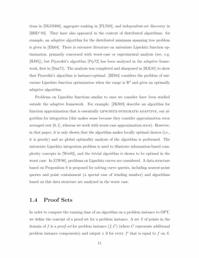
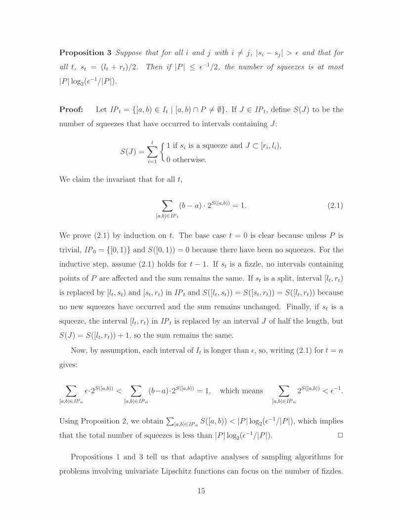
0 1P
fizzle squeeze split
s3 s2 s1
Figure 2-1: Different types of samples.
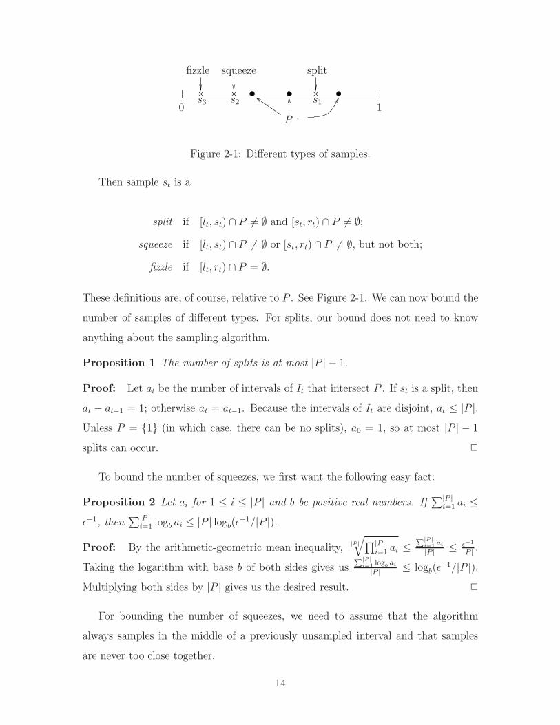
Then sample st is a
split if [lt, st) ∩ P 6= ∅ and [st, rt) ∩ P 6= ∅;
squeeze if [lt, st) ∩ P 6= ∅ or [st, rt) ∩ P 6= ∅, but not both;
fizzle if [lt, rt) ∩ P = ∅.
These definitions are, of course, relative to P . See Figure 2-1. We can now bound the
number of samples of different types. For splits, our bound does not need to know
anything about the sampling algorithm.
Proposition 1 The number of splits is at most |P | − 1.
Proof: Let at be the number of intervals of It that intersect P . If st is a split, then
at − at−1 = 1; otherwise at = at−1. Because the intervals of It are disjoint, at ≤ |P |.Unless P = 1 (in which case, there can be no splits), a0 = 1, so at most |P | − 1
splits can occur. 2
To bound the number of squeezes, we first want the following easy fact:
Proposition 2 Let ai for 1 ≤ i ≤ |P | and b be positive real numbers. If∑|P |
i=1 ai ≤ǫ−1, then
∑|P |i=1 logb ai ≤ |P | logb(ǫ
−1/|P |).
Proof: By the arithmetic-geometric mean inequality, |P |√
∏|P |i=1 ai ≤
P|P |i=1 ai
|P | ≤ ǫ−1
|P | .
Taking the logarithm with base b of both sides gives usP|P |
i=1 logb ai
|P | ≤ logb(ǫ−1/|P |).
Multiplying both sides by |P | gives us the desired result. 2
For bounding the number of squeezes, we need to assume that the algorithm
always samples in the middle of a previously unsampled interval and that samples
are never too close together.
14
Proposition 3 Suppose that for all i and j with i 6= j, |si − sj | > ǫ and that for
all t, st = (lt + rt)/2. Then if |P | ≤ ǫ−1/2, the number of squeezes is at most
|P | log2(ǫ−1/|P |).
Proof: Let IP t = [a, b) ∈ It | [a, b) ∩ P 6= ∅. If J ∈ IP t, define S(J) to be the
number of squeezes that have occurred to intervals containing J :
S(J) =
t∑
i=1
1 if si is a squeeze and J ⊂ [ri, li),
0 otherwise.
We claim the invariant that for all t,
∑
[a,b)∈IP t
(b− a) · 2S([a,b)) = 1. (2.1)
We prove (2.1) by induction on t. The base case t = 0 is clear because unless P is
trivial, IP0 = [0, 1) and S([0, 1)) = 0 because there have been no squeezes. For the
inductive step, assume (2.1) holds for t − 1. If st is a fizzle, no intervals containing
points of P are affected and the sum remains the same. If st is a split, interval [lt, rt)
is replaced by [lt, st) and [st, rt) in IP t and S([lt, st)) = S([st, rt)) = S([lt, rt)) because
no new squeezes have occurred and the sum remains unchanged. Finally, if st is a
squeeze, the interval [lt, rt) in IP t is replaced by an interval J of half the length, but
S(J) = S([lt, rt)) + 1, so the sum remains the same.
Now, by assumption, each interval of It is longer than ǫ, so, writing (2.1) for t = n
gives:
∑
[a,b)∈IPn
ǫ·2S([a,b)) <∑
[a,b)∈IPn
(b−a)·2S([a,b)) = 1, which means∑
[a,b)∈IPn
2S([a,b)) < ǫ−1.
Using Proposition 2, we obtain∑
[a,b)∈IPnS([a, b)) < |P | log2(ǫ
−1/|P |), which implies
that the total number of squeezes is less than |P | log2(ǫ−1/|P |). 2
Propositions 1 and 3 tell us that adaptive analyses of sampling algorithms for
problems involving univariate Lipschitz functions can focus on the number of fizzles.
15
x1 x2
f(x1)
Lf (x1, x2)
f
f
f(x2)
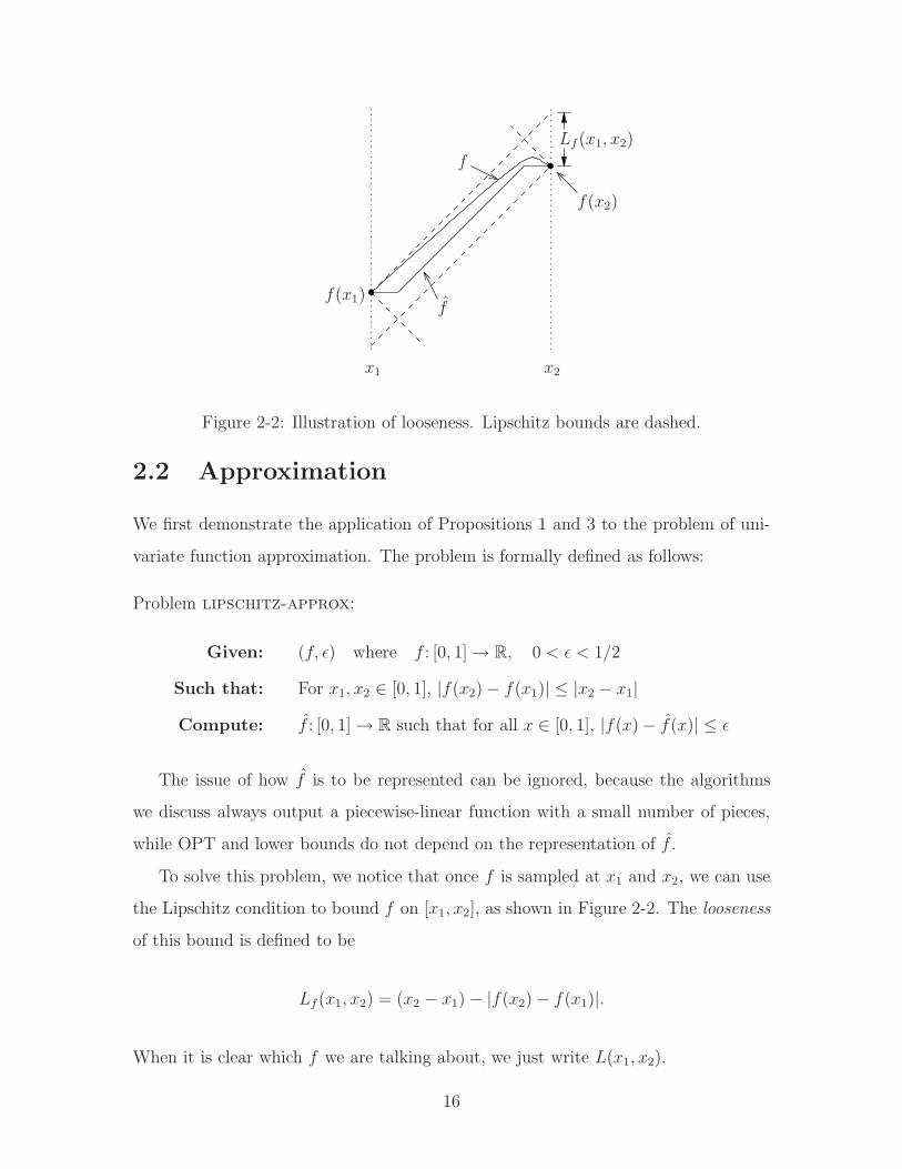
Figure 2-2: Illustration of looseness. Lipschitz bounds are dashed.
2.2 Approximation
We first demonstrate the application of Propositions 1 and 3 to the problem of uni-
variate function approximation. The problem is formally defined as follows:
Problem lipschitz-approx:
Given: (f, ǫ) where f : [0, 1]→ R, 0 < ǫ < 1/2
Such that: For x1, x2 ∈ [0, 1], |f(x2)− f(x1)| ≤ |x2 − x1|
Compute: f : [0, 1]→ R such that for all x ∈ [0, 1], |f(x)− f(x)| ≤ ǫ
The issue of how f is to be represented can be ignored, because the algorithms
we discuss always output a piecewise-linear function with a small number of pieces,
while OPT and lower bounds do not depend on the representation of f .
To solve this problem, we notice that once f is sampled at x1 and x2, we can use
the Lipschitz condition to bound f on [x1, x2], as shown in Figure 2-2. The looseness
of this bound is defined to be
Lf(x1, x2) = (x2 − x1)− |f(x2)− f(x1)|.
When it is clear which f we are talking about, we just write L(x1, x2).
16
Proposition 4 Given a Lipschitz function f , looseness has the following properties:
(1) 0 ≤ L(x1, x2) ≤ x2 − x1.
(2) If x′1 ≤ x1 < x2 ≤ x′
2 then L(x1, x2) ≤ L(x′1, x
′2).
Proof: This follows immediately from the definition of looseness and the Lipschitz
condition on f . 2
As the following proposition shows, the accuracy with which we can approximate
f on [x1, x2] given only the value of f at x1 and x2 is precisely L(x1, x2)/2.
Proposition 5 Let f : [0, 1]→ R be Lipschitz and let [x1, x2] be a subinterval of [0, 1].
Then:
(1) If HI (x) = min(f(x1) + |x−x1|, f(x2) + |x2−x|) and LO(x) = max(f(x1)− |x−x1|, f(x2) − |x2 − x|), the function defined as f(x) = (HI (x) + LO(x))/2 is within
L(x1, x2)/2 of f on [x1, x2].
(2) For any function f on [x1, x2], there is a Lipschitz function g and a point x ∈(x1, x2) such that g(x1) = f(x1), g(x2) = f(x2), and |f(x)− g(x)| ≥ L(x1, x2)/2.
Proof: First we show part (1). Notice that the Lipschitz condition on f implies
that LO(x) ≤ f(x) ≤ HI (x). This implies that at any x, |f(x)− f(x)| ≤ (HI (x) −LO(x))/2. Consider first the case f(x1) ≤ f(x2). Note that HI (x) ≤ f(x1) + x− x1
and LO(x) ≥ f(x2) + x− x2 which implies that
HI (x)− LO(x) ≤ x2 − x1 − (f(x2)− f(x1)) = L(x1, x2).
Similarly, for the case f(x1) > f(x2), we note that HI (x) ≤ f(x2) + x2 − x and
LO(x) ≥ f(x1)− x + x1 and so
HI (x)− LO(x) ≤ x2 − x1 − (f(x1)− f(x2)) = L(x1, x2).
Thus, |f(x)− f(x)| ≤ (HI (x)− LO(x))/2 ≤ L(x1, x2)/2, which proves part (1).
For part (2), note that both HI (x) and LO(x) are Lipschitz and HI (x1) =
LO(x1) = f(x1) and HI (x2) = LO(x2) = f(x2). Let x = (x1 + x2)/2 and note
17
that HI (x) = min(f(x1), f(x2))+(x2−x1)/2 and LO(x) = max(f(x1), f(x2))− (x2−x1)/2 so HI (x) − LO(x) = L(x1, x2). By the triangle inequality, |HI (x) − f(x)| +|LO(x) − f(x)| ≥ L(x1, x2), which implies that either |HI (x) − f(x)| ≥ L(x1, x2)/2
or |LO(x)− f(x)| ≥ L(x1, x2)/2. 2
Proposition 5 immediately gives the criterion for a proof set:
Corollary 1 Let P = x1, x2, . . . , xn such that 0 ≤ x1 < x2 < · · · < xn ≤ 1. Then
P is a proof set for problem instance (f, ǫ) if and only if x1 ≤ ǫ, xn ≥ 1− ǫ, and for
all i with 1 ≤ i ≤ n− 1, Lf(xi, xi+1) ≤ 2ǫ.
Proof: If x1 ≤ ǫ, xn ≥ 1− ǫ, and Lf (xi, xi+1) ≤ 2ǫ then f can be approximated to
within ǫ with f(x1) on [0, x1], f(xn) on [xn, 1], and a pasting of functions of the form
(HI (x) + LO(x))/2 as in Proposition 5(1).
In the other direction, if x1 > ǫ, f(0) could be anywhere in the range [f(x1) −x1, f(x1)+x1] and so no value of f(0) is guaranteed to be within ǫ of f(0). Similarly,
P cannot be a proof set if xn < 1− ǫ. If Lf (xi, xi+1) > 2ǫ for some i, Proposition 5(2)
shows that f cannot be approximated to within ǫ on (xi, xi+1). 2
The simplest way to obtain a proof set is to sample f at ǫ, 3ǫ, 5ǫ, . . . , 1−ǫ. Propo-
sition 4(1) guarantees that this is a proof set regardless of f . Thus, a trivial algorithm
can solve lipschitz-approx using O(ǫ−1) samples. On the other hand, if f(x) = 0
for all x, then Lf(x1, x2) = x2 − x1 for all x1 < x2, which implies that Ω(ǫ−1) sam-
ples are necessary for a proof set. So, as with most other problems we consider, the
worst-case scenario is simple and not very interesting for lipschitz-approx and we
now focus on adaptive algorithms.
Figure 2-3 gives an adaptive algorithm for this problem. We will show, using the
tools in Section 2.1, that this algorithm is optimally adaptive. The idea is to start
by sampling f at 0 and 1, and then sample inside previously unsampled intervals
where looseness is higher than 2ǫ until none are left. For bookkeeping, we store all of
the sampled points in a singly linked list, ordered by the parameter value. We also
maintain a “To-Do” stack which contains pointers to endpoints of intervals we have
18
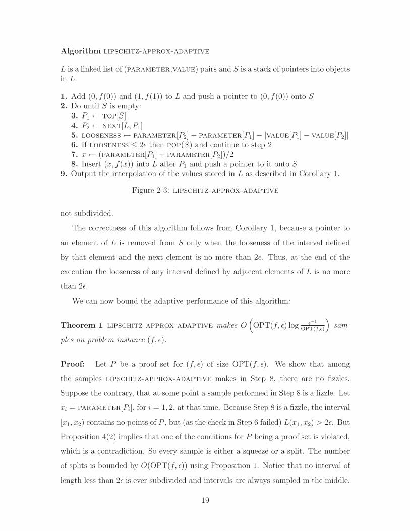
Algorithm lipschitz-approx-adaptive
L is a linked list of (parameter,value) pairs and S is a stack of pointers into objectsin L.
1. Add (0, f(0)) and (1, f(1)) to L and push a pointer to (0, f(0)) onto S2. Do until S is empty:
3. P1 ← top[S]4. P2 ← next[L, P1]5. looseness← parameter[P2]− parameter[P1]− |value[P1]− value[P2]|6. If looseness ≤ 2ǫ then pop(S) and continue to step 27. x← (parameter[P1] + parameter[P2])/28. Insert (x, f(x)) into L after P1 and push a pointer to it onto S
9. Output the interpolation of the values stored in L as described in Corollary 1.
Figure 2-3: lipschitz-approx-adaptive
not subdivided.
The correctness of this algorithm follows from Corollary 1, because a pointer to
an element of L is removed from S only when the looseness of the interval defined
by that element and the next element is no more than 2ǫ. Thus, at the end of the
execution the looseness of any interval defined by adjacent elements of L is no more
than 2ǫ.
We can now bound the adaptive performance of this algorithm:
Theorem 1 lipschitz-approx-adaptive makes O(
OPT(f, ǫ) log ǫ−1
OPT(f,ǫ)
)
sam-
ples on problem instance (f, ǫ).
Proof: Let P be a proof set for (f, ǫ) of size OPT(f, ǫ). We show that among
the samples lipschitz-approx-adaptive makes in Step 8, there are no fizzles.
Suppose the contrary, that at some point a sample performed in Step 8 is a fizzle. Let
xi = parameter[Pi], for i = 1, 2, at that time. Because Step 8 is a fizzle, the interval
[x1, x2) contains no points of P , but (as the check in Step 6 failed) L(x1, x2) > 2ǫ. But
Proposition 4(2) implies that one of the conditions for P being a proof set is violated,
which is a contradiction. So every sample is either a squeeze or a split. The number
of splits is bounded by O(OPT(f, ǫ)) using Proposition 1. Notice that no interval of
length less than 2ǫ is ever subdivided and intervals are always sampled in the middle.
19
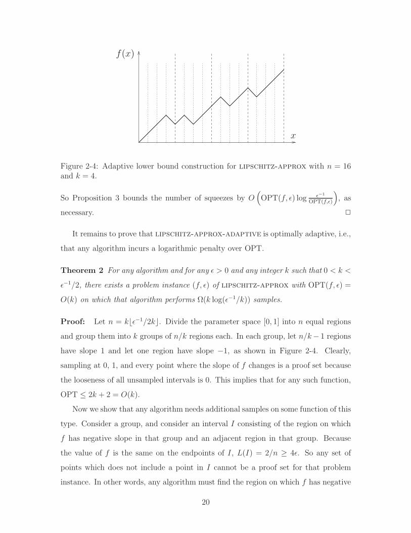
f(x)
x
Figure 2-4: Adaptive lower bound construction for lipschitz-approx with n = 16and k = 4.
So Proposition 3 bounds the number of squeezes by O(
OPT(f, ǫ) log ǫ−1
OPT(f,ǫ)
)
, as
necessary. 2
It remains to prove that lipschitz-approx-adaptive is optimally adaptive, i.e.,
that any algorithm incurs a logarithmic penalty over OPT.
Theorem 2 For any algorithm and for any ǫ > 0 and any integer k such that 0 < k <
ǫ−1/2, there exists a problem instance (f, ǫ) of lipschitz-approx with OPT(f, ǫ) =
O(k) on which that algorithm performs Ω(k log(ǫ−1/k)) samples.
Proof: Let n = k⌊ǫ−1/2k⌋. Divide the parameter space [0, 1] into n equal regions
and group them into k groups of n/k regions each. In each group, let n/k− 1 regions
have slope 1 and let one region have slope −1, as shown in Figure 2-4. Clearly,
sampling at 0, 1, and every point where the slope of f changes is a proof set because
the looseness of all unsampled intervals is 0. This implies that for any such function,
OPT ≤ 2k + 2 = O(k).
Now we show that any algorithm needs additional samples on some function of this
type. Consider a group, and consider an interval I consisting of the region on which
f has negative slope in that group and an adjacent region in that group. Because
the value of f is the same on the endpoints of I, L(I) = 2/n ≥ 4ǫ. So any set of
points which does not include a point in I cannot be a proof set for that problem
instance. In other words, any algorithm must find the region on which f has negative
20
slope in every group, or an adjacent one. The endpoints of the groups are the same
for all functions of this type, so sampling in one group provides no information about
the location of negative-slope regions in other groups. Therefore each search for the
negative-slope region must be done independently. Moreover, sampling inside a group
only gives information as to whether the negative-slope region is to the left or to the
right of the sampled point. This means that the problem in every group is as hard
as a continuous binary search on an interval of length 1/k for a region of length 2/n,
which requires Ω(log(n/k)) time in the worst case. The algorithm needs to perform
k independent such searches, giving the desired lower bound. 2
2.3 Integration
We now turn to the problem of univariate integration. The problem is formulated as
follows:
Problem lipschitz-integrate:
Given: (f, ǫ), where f : [0, 1]→ R, 0 < ǫ < 1/2
Such that: For x1, x2 ∈ [0, 1], |f(x2)− f(x1)| ≤ |x2 − x1|
Compute: M ∈ R such that
∣
∣
∣
∣
M −∫ 1
0
f(x) dx
∣
∣
∣
∣
≤ ǫ
At first glance, it seems that integration can be reduced to approximation. In-
deed, given a black box for f on [0, 1], if we know explicitly a function f that is
guaranteed to be within ǫ of f everywhere, then the integral of f must be within
ǫ of the true integral of f . Thus, every proof set for approximation is also a proof
set for integration, and lipschitz-approx-adaptive can be trivially transformed
to solve lipschitz-integrate. The resulting algorithm is not optimally adaptive,
however. This is because OPT for integration can be asymptotically smaller than
21
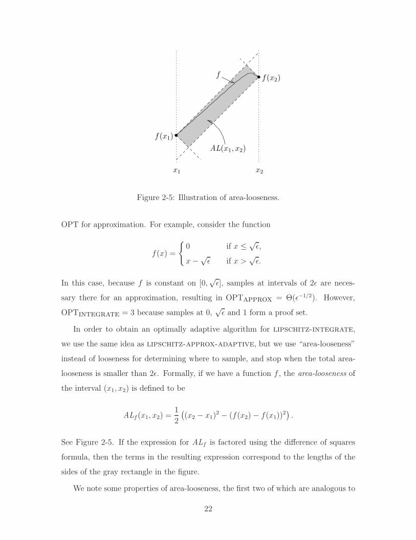
x1 x2
f(x1)
f f(x2)
AL(x1, x2)
Figure 2-5: Illustration of area-looseness.
OPT for approximation. For example, consider the function
f(x) =
0 if x ≤ √ǫ,
x−√ǫ if x >√
ǫ.
In this case, because f is constant on [0,√
ǫ], samples at intervals of 2ǫ are neces-
sary there for an approximation, resulting in OPTapprox = Θ(ǫ−1/2). However,
OPTintegrate = 3 because samples at 0,√
ǫ and 1 form a proof set.
In order to obtain an optimally adaptive algorithm for lipschitz-integrate,
we use the same idea as lipschitz-approx-adaptive, but we use “area-looseness”
instead of looseness for determining where to sample, and stop when the total area-
looseness is smaller than 2ǫ. Formally, if we have a function f , the area-looseness of
the interval (x1, x2) is defined to be
ALf (x1, x2) =1
2
(
(x2 − x1)2 − (f(x2)− f(x1))
2)
.
See Figure 2-5. If the expression for ALf is factored using the difference of squares
formula, then the terms in the resulting expression correspond to the lengths of the
sides of the gray rectangle in the figure.
We note some properties of area-looseness, the first two of which are analogous to
22

looseness properties in Proposition 4:
Proposition 6 Area-Looseness has the following properties:
(1) 0 ≤ AL(x1, x2) ≤ (x2 − x1)2/2.
(2) If x′1 ≤ x1 < x2 ≤ x′
2 then AL(x1, x2) ≤ AL(x′1, x
′2).
(3) If x ∈ [x1, x2], then AL(x1, x) + AL(x, x2) ≤ AL(x1, x2).
(4) AL(
x1,x1+x2
2
)
+ AL(
x1+x2
2, x2
)
≤ AL(x1, x2)/2.
Proof: Part (1) is obvious, and (2) follows from (3), so we prove (3) and (4):
(3) The Lipschitz condition implies that |x1−x| ≥ |f(x1)− f(x)| and |x2−x| ≥|f(x2)− f(x)|, and therefore |(x1 − x)(x2 − x)| ≥ |(f(x1)− f(x))(f(x2)− f(x))|. In
addition, (x1 − x)(x2 − x) ≤ 0, so (f(x1)− f(x))(f(x2)− f(x)) ≥ (x1 − x)(x2 − x).
Multiplying through, we get
f(x1)f(x2) + f(x)2 − f(x1)f(x)− f(x2)f(x) ≥ x1x2 + x2 − xx1 − xx2.
Rearranging, we get
−x1x2 + f(x1)f(x2) ≥ x2 − xx1 − xx2 − f(x)2 + f(x)f(x1) + f(x)f(x2).
Addingx22+x2
1+f(x1)2+f(x2)2
2to both sides to complete the squares, we get
(x2 − x1)2 − (f(x1)− f(x2))
2
2≥
≥ (x− x1)2 − (f(x1)− f(x))2
2+
(x2 − x)2 − (f(x2)− f(x))2
2.
By the definition of AL, this inequality is equivalent to (3).
(4) Let xm = (x1 + x2)/2. The proposition claims that if f is Lipschitz,
(x2 − x1)2 − (f(x2)− f(x1))
2
2≥
≥ (xm − x1)2−(f(xm)− f(x1))
2 + (x2 − xm)2 − (f(x2)− f(xm))2.
23
Because (xm − x1) = (x2 − xm) = (x2 − x1)/2, the claim can be written as
(x2 − x1)2 − (f(x2)− f(x1))
2
2≥ (x2 − x1)
2
2− (f(xm)− f(x1))
2 − (f(x2)− f(xm))2.
Thus, we need to show that
(f(x2)− f(x1))2 ≤ 2(f(xm)− f(x1))
2 + 2(f(x2)− f(xm))2.
Notice that the right-hand side can be written as af(xm)2 + bf(xm) + c, where a = 4
and b = −4f(x1)− 4f(x2). This expression has a single global minimum at f(xm) =
−b/2a, which is fm = (f(x1) + f(x2))/2. Therefore, we have:
2(fm − f(x1))2 + 2(f(x2)− fm)2 ≤ 2(f(xm)− f(x1))
2 + 2(f(x2)− f(xm))2.
But we can rewrite the left-hand side as:
2
(
f(x2)− f(x1)
2
)2
+ 2
(
f(x2)− f(x1)
2
)2
= (f(x2)− f(x1))2,
which gives us the claim. 2
We now need to show that area-looseness is the right property for bounding the
accuracy of an integral approximation on an interval. To do this, we prove an analogue
of Proposition 5:
Proposition 7 Let f : [0, 1]→ R be Lipschitz and let [x1, x2] be a subinterval of [0, 1].
Then:
(1)∣
∣
∣(x2 − x1) · f(x1)+f(x2)
2−∫ x2
x1f(x) dx
∣
∣
∣≤ AL(x1, x2)/2.
(2) For any M ∈ R, there is a Lipschitz function g such that g(x1) = f(x1), g(x2) =
f(x2), and∣
∣
∣M −
∫ x2
x1g(x) dx
∣
∣
∣≥ AL(x1, x2)/2.
Proof: For part (1), define the functions HI (x) = min(f(x1)+ |x−x1|, f(x2)+ |x2−x|) and LO(x) = max(f(x1)− |x− x1|, f(x2)− |x2− x|). By the Lipschitz condition,
24
LO(x) ≤ f(x) ≤ HI (x) on [x1, x2]. Therefore,
∫ x2
x1
LO(x) dx ≤∫ x2
x1
f(x) dx ≤∫ x2
x1
HI (x) dx
so
∣
∣
∣
∣
∫ x2
x1
LO(x) + HI (x)
2dx−
∫ x2
x1
f(x) dx
∣
∣
∣
∣
≤ 1
2
(∫ x2
x1
HI (x) dx−∫ x2
x1
LO(x) dx
)
.
Note that f(x1)+x−x1 ≤ f(x2)+x2−x precisely when x ≤ (f(x2)−f(x1)+x1+x2)/2.
Therefore, we have
∫ x2
x1
HI (x) dx =
∫ (f(x2)−f(x1)+x1+x2)/2
x1
(f(x1) + x− x1) dx +
+
∫ x2
(f(x2)−f(x1)+x1+x2)/2
(f(x2) + x2 − x) dx =
=3f(x1) + f(x2) + x2 − x1
4· f(x2)− f(x1) + (x2 − x1)
2+
+f(x1) + 3f(x2) + x2 − x1
4· f(x1)− f(x2) + (x2 − x1)
2=
= f(x1) ·f(x2)− f(x1) + (x2 − x1)
4+ f(x2) ·
f(x1)− f(x2) + (x2 − x1)
4+
+f(x1) + f(x2) + x2 − x1
4· (x2 − x1) =
= (x2 − x1)f(x1) + f(x2)
2+
(f(x2)− f(x1))(f(x1)− f(x2))
4+
(x2 − x1)2
4=
= (x2 − x1)f(x1) + f(x2)
2+ AL(x1, x2)/2.
Similarly,∫ x2
x1LO(x) dx = (x2 − x1)
f(x1)+f(x2)2
− AL(x1, x2)/2. Substituting the inte-
grals for HI and LO gives the inequality of (1).
To show part (2), notice that both HI and LO are Lipschitz and HI (x1) =
LO(x1) = f(x1) and HI (x2) = LO(x2) = f(x2). If M ≥∫ x2
x1
LO(x)+HI (x)2
dx, let
25

g(x) = LO(x); otherwise let g(x) = HI (x). Then
∣
∣
∣
∣
M −∫ x2
x1
g(x) dx
∣
∣
∣
∣
≥ 1
2
(∫ x2
x1
HI (x) dx−∫ x2
x1
LO(x) dx
)
=1
2·AL(x1, x2).
and (2) follows. 2
We can now formulate the criterion for a proof set for lipschitz-integrate:
Corollary 2 Let P = x1, x2, . . . , xn such that 0 ≤ x1 < x2 < · · · < xn ≤ 1.
Then P is a proof set for problem instance (f, ǫ) if and only if x21 + (1 − xn)2 +
∑n−1i=1 AL(xi, xi+1) ≤ 2ǫ.
Proof: The value M = x1 ·f(x1)+(1−xn)·f(xn)+∑n−1
i=1
(
(xi+1 − xi) · f(xi)+f(xi+1)2
)
is within ǫ of∫ 1
0f(x) dx because
∣
∣
∣
∣
x1 · f(x1)−∫ x1
0
f(x) dx
∣
∣
∣
∣
≤ x21
2,
∣
∣
∣
∣
(1− xn) · f(xn)−∫ 1
xn
f(x) dx
∣
∣
∣
∣
≤ (1− xn)2
2,
and for each i,∣
∣
∣(xi+1 − xi) · f(xi)+f(xi+1)
2−∫ xi+1
xif(x) dx
∣
∣
∣≤ 1
2·AL(xi, xi+1) by Propo-
sition 7.
In the other direction, if x21 + (1 − xn)2 +
∑n−1i=1 AL(xi, xi+1) > 2ǫ, then two
functions, fHI and fLO , can be constructed such that fHI (xi) = f(xi) = fLO(xi)
but∫ 1
0fHI (x) dx −
∫ 1
0fLO(x) dx > 2ǫ, which means that no matter what value an
algorithm outputs after sampling P , that value will be incorrect for either fHI or
fLO . 2
This corollary, together with Proposition 6, immediately shows the correctness
of a trivial algorithm. Let n = ⌈ǫ−1/4⌉ and let the algorithm make n samples, at
12n
, 32n
, . . . , 2n−12n
and output the integral M as in the proof of Corollary 2. It is correct
because the area-looseness of every interval is at most (1/n)2/2. Because there are
n− 1 intervals, the total area-looseness of all of them is at most (n− 1)/(2n2). Also,
x21 = (1 − xn)2 = 1/(2n)2, so x2
1 + (1 − xn)2 +∑n−1
i=1 AL(xi, xi+1) = n/(2n2) ≤ 2ǫ.
Therefore, as in lipschitz-approx, Θ(ǫ−1) samples are always sufficient (and if, for
instance, f is constant, necessary).
26
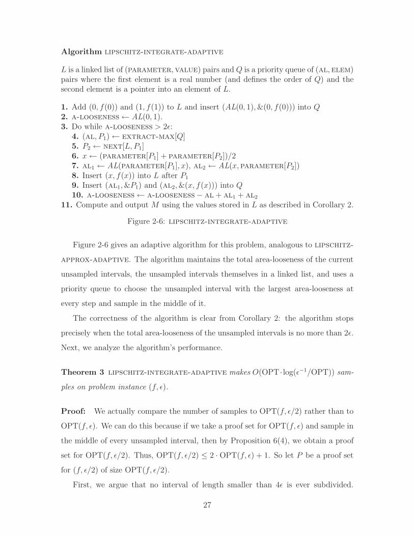
Algorithm lipschitz-integrate-adaptive
L is a linked list of (parameter,value) pairs and Q is a priority queue of (al, elem)pairs where the first element is a real number (and defines the order of Q) and thesecond element is a pointer into an element of L.
1. Add (0, f(0)) and (1, f(1)) to L and insert (AL(0, 1), &(0, f(0))) into Q2. a-looseness← AL(0, 1).3. Do while a-looseness > 2ǫ:
4. (al, P1)← extract-max[Q]5. P2 ← next[L, P1]6. x← (parameter[P1] + parameter[P2])/27. al1 ← AL(parameter[P1], x), al2 ← AL(x, parameter[P2])8. Insert (x, f(x)) into L after P1
9. Insert (al1, &P1) and (al2, &(x, f(x))) into Q10. a-looseness← a-looseness− al + al1 + al2
11. Compute and output M using the values stored in L as described in Corollary 2.
Figure 2-6: lipschitz-integrate-adaptive
Figure 2-6 gives an adaptive algorithm for this problem, analogous to lipschitz-
approx-adaptive. The algorithm maintains the total area-looseness of the current
unsampled intervals, the unsampled intervals themselves in a linked list, and uses a
priority queue to choose the unsampled interval with the largest area-looseness at
every step and sample in the middle of it.
The correctness of the algorithm is clear from Corollary 2: the algorithm stops
precisely when the total area-looseness of the unsampled intervals is no more than 2ǫ.
Next, we analyze the algorithm’s performance.
Theorem 3 lipschitz-integrate-adaptive makes O(OPT · log(ǫ−1/OPT)) sam-
ples on problem instance (f, ǫ).
Proof: We actually compare the number of samples to OPT(f, ǫ/2) rather than to
OPT(f, ǫ). We can do this because if we take a proof set for OPT(f, ǫ) and sample in
the middle of every unsampled interval, then by Proposition 6(4), we obtain a proof
set for OPT(f, ǫ/2). Thus, OPT(f, ǫ/2) ≤ 2 ·OPT(f, ǫ) + 1. So let P be a proof set
for (f, ǫ/2) of size OPT(f, ǫ/2).
First, we argue that no interval of length smaller than 4ǫ is ever subdivided.
27
Suppose for contradiction that among n intervals I1, . . . , In of lengths a1, . . . , an,
interval Ik with ak < 4ǫ is chosen for subdivision. By Proposition 6(1), AL(Ii) ≤ a2i /2,
so√
AL(Ik)/2 ≤ 2ǫ. On the other hand,∑
ai = 1, so∑
√
2AL(Ii) ≤ 1. Multiplying
the inequalities, we get∑
AL(Ii) ≤∑
√
AL(Ii)AL(Ik) ≤ 2ǫ. But this implies that
the algorithm should have terminated, which is a contradiction.
Now, we count the number of samples relative to P . The number of splits is
O(|P |) by Proposition 1. The above paragraph shows that we can use Proposition 3
to conclude that there are O(|P | log(ǫ−1/|P |)) squeezes. This does not conclude
the analysis because, unlike for the approximation problem, fizzles are now possible.
However, we now show that there are O(|P |) fizzles, proving the theorem.
A fizzle occurs when an interval not containing a point of P is chosen for subdi-
vision. Consider the situation after n points have been sampled. Let the sampled
points be 0 = x1 ≤ x2 ≤ · · · ≤ xn = 1. Because the total area-looseness of intervals
between points of P is at most ǫ, by repeated application of Proposition 6(2,3), we
have∑
[xi,xi+1)∩P=∅AL(xi, xi+1) ≤ ǫ.
The algorithm has not terminated, so the total area-looseness must be more than 2ǫ,
which implies that∑
[xi,xi+1)∩P 6=∅AL(xi, xi+1) > ǫ.
Because there are at most |P | elements in the sum on the left-hand side, the largest
element must be greater than ǫ/|P |. Therefore, there exists a k such that [xk, xk+1)
contains a point of P and AL(xk, xk+1) > ǫ/|P |. The algorithm always chooses the
interval with the largest area looseness, so if a fizzle occurs, the area-looseness of the
chosen interval must be at least ǫ/|P |.
Now let St be the set of samples made by the algorithm after time t. Define
At as follows: let y1, y2, . . . , yn = St ∪ P with 0 = y1 ≤ y2 ≤ · · · ≤ yn and let
At =∑n−1
i=1 AL(yi, yi+1). Clearly, At ≥ 0, At ≥ At+1 (by Proposition 6(3)), and
therefore, At ≤ A0 ≤ 2ǫ. Every fizzle splits an interval between adjacent y’s into
28
two. Because the area-looseness of the interval before the split was at least ǫ/|P |,by Proposition 6(4), At decreases by at least ǫ/(2|P |) as a result of every fizzle.
Therefore, there can be at most 4|P | fizzles during an execution. 2
We now prove a matching lower bound that shows that the logarithmic factor is
necessary and that lipschitz-integrate-adaptive is optimally adaptive:
Theorem 4 For any deterministic algorithm and for any ǫ > 0 and any integer
k such that 0 < k < ǫ−1/2, there exists a problem instance (f, ǫ) of lipschitz-
integrate with OPT(f, ǫ) = O(k) on which that algorithm performs Ω(k log(ǫ−1/k))
samples.
Proof: The proof is very similar to the proof of Theorem 2. The construction
is essentially the same, but with different constants. Let n = k⌊1/√
2ǫk⌋. Divide
the parameter space [0, 1] into n equal regions and group them into k groups of n/k
regions each. In each group, let n/k − 1 regions have slope 1 and let 1 region have
slope −1 (see Figure 2-4 for an illustration). As with approximation, sampling at
0, 1, and every point where the slope of f changes is a proof set because the area
looseness of all unsampled intervals is 0. This implies that for any such function,
OPT ≤ 2k + 2 = O(k).
Now we show that any algorithm needs additional samples on some function of this
type. Consider a group, and consider an interval I consisting of the region on which
f has negative slope in that group and an adjacent region in that group. Because the
value of f is the same on the endpoints of I, AL(I) = 2/n2 ≥ 4ǫ/k. Therefore, an
algorithm that does not find the negative-slope region or an adjacent one in at least
k/2 groups will not be correct on some inputs. Finding the negative-slope region in
each group is a binary search that needs Ω(log(n/k)) = Ω(log(ǫ−1/k)) samples and
this needs to be done independently for Ω(k) groups, giving us the bound. 2
The above theorem shows that lipschitz-integrate-adaptive cannot be im-
proved by more than a constant factor with respect to the number of samples. How-
ever, notice that in addition to sampling f , the algorithm maintains numbers in a
29
priority queue Q. If Q is implemented as a heap, then an execution that makes n
samples requires an additional O(n logn) time for the extract-max operations on Q.
In fact, this logarithmic overhead can be avoided. The key to eliminating this
overhead is to observe that a strict priority queue is not required for the algorithm. As
long as the extract-max operation guarantees that the value of the element extracted
is at least half (or any constant factor) of the maximum value stored in Q, the proof
of Theorem 3 holds (although the constants increase). Therefore, an approximate
priority queue is sufficient. Furthermore, notice that the queue stores area-loosenesses
of unsampled intervals, which can vary from 0 to 1. However, if n is the number of
samples made by the algorithm, then no interval whose area-looseness is smaller than
2ǫ/n is ever subdivided, and because n is no more than ǫ−1, the queue only needs to
store numbers between 2ǫ2 and 1. Finally, notice that the maximum value in Q is
always decreasing.
The above observations allow us to implement Q so that all operations can be
done in O(n + log(1/ǫ)) time. The implementation consists of k buckets numbered
1 through k, where k = ⌊log2(ǫ−2)⌋ and a variable that initially points to bucket 1.
Bucket i stores values in the range [2−i, 21−i). An insert operation simply inserts the
value into the proper bucket. An extract-max operation first increments the variable
until it points to a non-empty bucket and then extracts any value from that bucket.
Insertion takes constant time per operation (assuming that computing the floor of
the log of a number takes constant time) and extraction takes constant time plus the
time to increment the variable. Since there are only Θ(log(1/ǫ)) buckets, the total
time for all of the operations is O(n + log(1/ǫ)).
30

Chapter 3
Functions from R to Rd
3.1 Lipschitz Curves
When the range of a univariate Lipschitz function is Rd with d > 1, such a function
is a parametric curve. The study of adaptive algorithms on Lipschitz curves was
initiated in [BD04]. In this thesis, we apply similar techniques to different problems.
The observation that leads to the algorithms is that once two points on a curve are
sampled, the curve between these two points must lie inside an ellipse. The following
three propositions (proved in [BD04]) formalize this idea.
Given a Lipschitz curve C and an interval [x1, x2] ⊆ [0, 1], define the ellipse
EC(x1, x2) =
p ∈ Rd∣
∣
∣‖C(x1)− p‖+ ‖C(x2)− p‖ ≤ x2 − x1
.
See Figure 3-1.
EC(x1, x2)
C(x1) C(x2)
Figure 3-1: Some possible curves C inside an ellipse.
31
Proposition 8 For an interval J = [x1, x2] ⊆ [0, 1], C(J) ⊆ EC(x1, x2).
Proposition 9 Let J = (x1, x2) ⊆ [0, 1] and let C be a Lipschitz curve. Then for
every point p in EC(x1, x2), there is a Lipschitz curve C ′ such that C(x) = C ′(x) for
x 6∈ J and for some x ∈ J , C ′(x) = p.
Proposition 10 If J ′ = [x′1, x
′2] and J = [x1, x2] and J ′ ⊆ J , then EC(x′
1, x′2) ⊆
EC(x1, x2).
3.2 Approximation
We now consider the approximation problem when the range of the function is Rd.
There is no fundamental difference from the one-dimensional case. We can even
generalize lipschitz-approx-adaptive and Theorem 1 to the setting where the
range is an arbitrary metric space M (with metric dM). We define the generalized
looseness as follows: Let f : [0, 1]→M be a function, let G(x1,x2) be the set of Lipschitz
functions equal to f on [0, x1] and on [x2, 1], and let H be the set of all functions from
[0, 1] to M . Define
GLf (x1, x2) = minh∈H
maxg∈G(x1,x2)
maxx∈[x1,x2]
dM(g(x), h(x)).
In other words, GL is the maximum possible error on [x1, x2] of the best possible
approximator, h. Note that for M = R, generalized looseness is precisely half of
regular looseness. Note also that like looseness, GL does not depend on f other than
at x1 and x2, so computing GL does not require additional samples.
In order to get an algorithm for solving lipschitz-approx when the range of
f is M , we modify lipschitz-approx-adaptive to compute GL instead of L in
Step 5, to compare GL to ǫ in step 6, and to output a pasting of the best-possible
approximators (the h’s) in Step 9. Correctness follows from the definition of GL: the
algorithm stops only when there is a function that approximates f with error ǫ on
every interval.
32
We now analyze the performance of the modified algorithm. We start by proving
an analogue of the first part of Proposition 4 for GL:
Proposition 11 Given f , and an interval [x1, x2], 0 ≤ GL(x1, x2) ≤ (x2 − x1)/2.
Proof: Since dM ≥ 0, GL(x1, x2) ≥ 0. For the second inequality, let xm = (x1 +
x2)/2 and let h(x) = f(x1) for x ≤ xm and h(x) = f(x2) for x > xm. Now consider
any Lipschitz function g with g(x1) = f(x1) and g(x2) = f(x2) and consider any
point x ∈ [x1, x2]. If x ≤ xm, then
dM(g(x), h(x)) = dM(g(x), f(x1)) ≤ dM(g(x1), g(x)) + dM(g(x1), f(x1)) ≤
≤ |x− x1|+ 0 ≤ xm − x1 = (x2 − x1)/2.
Similarly, if x > xm, we also get dM(g(x), h(x)) ≤ (x2−x1)/2. Therefore, there exists
an h such that for any g and x, the error is smaller than (x2 − x1)/2. 2
We are now ready to prove that the algorithm is within a logarithmic factor of
OPT. The proof is analogous to that of Theorem 1.
Theorem 5 The modified algorithm for approximation uses O(OPT · log(ǫ−1/OPT))
samples on problem instance (f, ǫ).
Proof: Let P be a set of points that OPT samples on (f, ǫ). By Proposition 11,
no interval of length smaller than 2ǫ is ever subdivided. Therefore, by Propositions 1
and 3, the number of splits and squeezes is O(|P | log(ǫ−1/|P |)). We now show that
there are no fizzles.
Suppose, for contradiction, that the algorithm samples in the interval (x1, x2), but
there are no points of P in that interval. It must be the case that GL(x1, x2) > ǫ,
because otherwise the modified algorithm would not sample there. Now let h be the
function that OPT outputs. By definition of GL, there exists a Lipschitz g that is
equal to f everywhere except possibly on (x1, x2), such that dM(g(x), h(x)) > ǫ for
some x. But then if OPT is given the problem instance (g, ǫ), it would also output h
because f and g are the same everywhere OPT samples, but h would not be a correct
output. 2
33
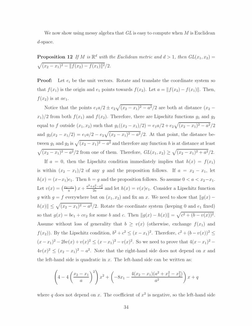
We now show using messy algebra that GL is easy to compute when M is Euclidean
d-space.
Proposition 12 If M is Rd with the Euclidean metric and d > 1, then GL(x1, x2) =
√
(x2 − x1)2 − ‖f(x2)− f(x1)‖2/2.
Proof: Let ei be the unit vectors. Rotate and translate the coordinate system so
that f(x1) is the origin and e1 points towards f(x2). Let a = ‖f(x2)− f(x1)‖. Then,
f(x2) is at ae1.
Notice that the points e1a/2 ± e2
√
(x2 − x1)2 − a2/2 are both at distance (x2 −x1)/2 from both f(x1) and f(x2). Therefore, there are Lipschitz functions g1 and g2
equal to f outside (x1, x2) such that g1((x2− x1)/2) = e1a/2 + e2
√
(x2 − x1)2 − a2/2
and g2(x2 − x1/2) = e1a/2 − e2
√
(x2 − x1)2 − a2/2. At that point, the distance be-
tween g1 and g2 is√
(x2 − x1)2 − a2 and therefore any function h is at distance at least√
(x2 − x1)2 − a2/2 from one of them. Therefore, GL(x1, x2) ≥√
(x2 − x1)2 + a2/2.
If a = 0, then the Lipschitz condition immediately implies that h(x) = f(x1)
is within (x2 − x1)/2 of any g and the proposition follows. If a = x2 − x1, let
h(x) = (x−x1)e1. Then h = g and the proposition follows. So assume 0 < a < x2−x1.
Let v(x) =(
x2−x1
a
)
x +a2+x2
1−x22
2aand let h(x) = v(x)e1. Consider a Lipschitz function
g with g = f everywhere but on (x1, x2) and fix an x. We need to show that ‖g(x)−h(x)‖ ≤
√
(x2 − x1)2 − a2/2. Rotate the coordinate system (keeping 0 and e1 fixed)
so that g(x) = be1 + ce2 for some b and c. Then ‖g(x)− h(x)‖ =√
c2 + (b− v(x))2.
Assume without loss of generality that b ≥ v(x) (otherwise, exchange f(x1) and
f(x2)). By the Lipschitz condition, b2 + c2 ≤ (x− x1)2. Therefore, c2 + (b− v(x))2 ≤
(x−x1)2− 2bv(x)+ v(x)2 ≤ (x−x1)
2− v(x)2. So we need to prove that 4(x−x1)2−
4v(x)2 ≤ (x2 − x1)2 − a2. Note that the right-hand side does not depend on x and
the left-hand side is quadratic in x. The left-hand side can be written as:
(
4− 4
(
x2 − x1
a
)2)
x2 +
(
−8x1 −4(x2 − x1)(a
2 + x21 − x2
2)
a2
)
x + q
where q does not depend on x. The coefficient of x2 is negative, so the left-hand side
34

has a global maximum at
(
8x1 +4(x2−x1)(a2+x2
1−x22)
a2
)
(
8− 8(
x2−x1
a
)2) =
x1a2 + (x2 − x1)(a
2 + x21 − x2
2)/2
a2 − (x2 − x1)2=
=x1a
2 + x2a2 + (x2 − x1)(x
21 − x2
2)
2(a2 − (x2 − x1)2)=
x1 + x2
2.
But at x = (x1 + x2)/2, v(x) = a/2, so 4(x− x1)2− 4v(x)2 = (x2 − x1)
2− a2 and the
proposition holds. 2
Finally, we note that Theorem 2, the lower bound on adaptive approximation
algorithms, carries over without modification to d > 1. Therefore, the modified
approximation algorithm is optimally adaptive.
3.3 Winding Number
We now consider the problem of computing the winding number of a curve in two
dimensions around a given point (which is assumed to be the origin).
Problem winding-number:
Given: C: [0, 1]→ R2
Such that: C(0) = C(1), for all x ∈ [0, 1], C(x) 6= 0,
and for x1, x2 ∈ [0, 1], ‖C(x2)− C(x1)‖ ≤ |x2 − x1|
Compute: The winding number of C around the origin
We first characterize proof sets for winding-number.
Proposition 13 Let P = x1, x2, . . . , xn with 0 = x1 < x2 < · · · < xn = 1. P is a
proof set for problem instance C if and only if for all i the origin is not in the interior
of EC(xi, xi+1).
Proof: First we show that if no ellipse interior contains the origin, P is a proof
set. Given a curve C ′ with C ′(xi) = C(xi), let H : [0, 1] × [0, 1] → R2 be defined
35
by H(x, t) = t · C ′(x) + (1− t) · C(x). Clearly H is a homotopy between C and C ′.
Suppose that H(x, t) = 0 for some x and t. Let xk and xk+1 be consecutive points in
P such that xk ≤ x ≤ xk+1. If xk+1 − xk = ‖C(xk+1) − C(xk)‖, then C ′(x) = C(x)
and by assumption, the image of C does not contain the origin. Otherwise C ′(x) 6= 0,
C(x) 6= 0 and both C ′(x) and C(x) are points in EC(xk, xk+1). Because EC is convex
and its boundary does not contain any line segments, no convex combination of
C ′(x) and C(x) contains the origin, contradicting the assumption that H(x, t) = 0.
Therefore, C ′ and C have a homotopy in R2 − 0 and hence the same winding
number. In particular, C ′ can be a parameterization of the polygon with vertices at
C(xi), so that polygon has the same winding number as C.
Conversely, if the origin is in the interior of EC(xk, xk+1), we show that there
are two Lipschitz functions, C1 and C2 such that C1(xi) = C2(xi) = C(xi) but C1
and C2 have different winding numbers. Let C1 = C2 = C everywhere except on
(xk, xk+1). Now let a = xk+1 − xk − ‖C(xk+1)‖ − ‖C(xk)‖. Because the interior of
EC(xk, xk+1) contains the origin, a > 0. Let p be a point such that ‖p‖ ≤ a/14
and such that p is not on the line segment between C(xk) and the origin nor on
the line segment between C(xk+1) and the origin. Then by the triangle inequality,
‖C(xk) − p‖ + ‖C(xk+1) − p‖ ≤ xk+1 − xk − a/7. Now let C1 on (xk, xk+1) consist
of the line segment from C(xk) to p followed by the line segment from p to C(xk+1).
Let C2 on (xk, xk+1) consist of the line segment from C(xk) to p, followed by the
counterclockwise circle of radius a/14 (arclength smaller than a/2) around the origin
followed by the line segment from p to C(xk+1). See Figure 3-2. Then the winding
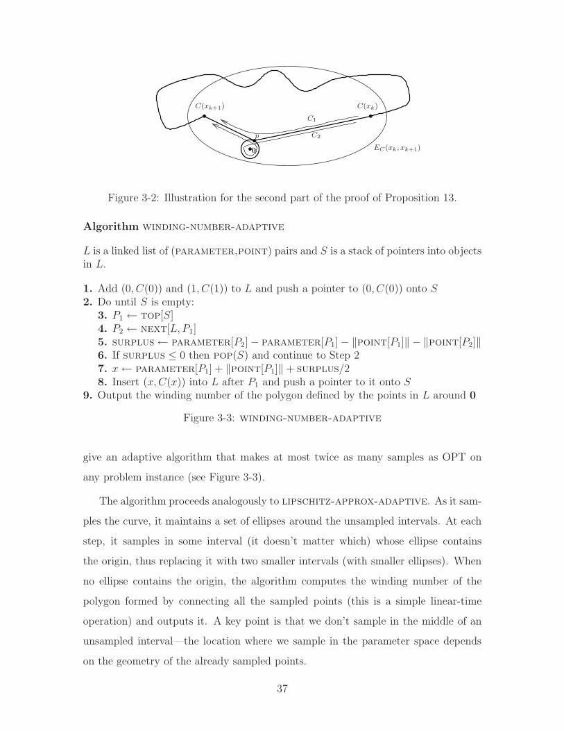
number of C2 is one greater than that of C1. 2
A set of points may be a proof set even if it doesn’t contain 0 or 1, but the
smallest proof set that does contain 0 and 1 has at most two points more than the
overall smallest proof set.
Notice that no bound on the number of samples necessary for this problem can be
given without knowing C. If C is contained in a disk of radius ǫ around the origin,
Ω(1/ǫ) samples are necessary to determine the winding number. However, we can
36
C(xk)
p
0
C1
C2
C(xk+1)
EC(xk , xk+1)
Figure 3-2: Illustration for the second part of the proof of Proposition 13.
Algorithm winding-number-adaptive
L is a linked list of (parameter,point) pairs and S is a stack of pointers into objectsin L.
1. Add (0, C(0)) and (1, C(1)) to L and push a pointer to (0, C(0)) onto S2. Do until S is empty:
3. P1 ← top[S]4. P2 ← next[L, P1]5. surplus← parameter[P2]− parameter[P1]− ‖point[P1]‖ − ‖point[P2]‖6. If surplus ≤ 0 then pop(S) and continue to Step 27. x← parameter[P1] + ‖point[P1]‖+ surplus/28. Insert (x, C(x)) into L after P1 and push a pointer to it onto S
9. Output the winding number of the polygon defined by the points in L around 0
Figure 3-3: winding-number-adaptive
give an adaptive algorithm that makes at most twice as many samples as OPT on
any problem instance (see Figure 3-3).
The algorithm proceeds analogously to lipschitz-approx-adaptive. As it sam-
ples the curve, it maintains a set of ellipses around the unsampled intervals. At each
step, it samples in some interval (it doesn’t matter which) whose ellipse contains
the origin, thus replacing it with two smaller intervals (with smaller ellipses). When
no ellipse contains the origin, the algorithm computes the winding number of the
polygon formed by connecting all the sampled points (this is a simple linear-time
operation) and outputs it. A key point is that we don’t sample in the middle of an
unsampled interval—the location where we sample in the parameter space depends
on the geometry of the already sampled points.
37

The algorithm is correct because it only stops subdividing an interval once the
ellipse around it does not contain the origin (i.e. surplus ≤ 0) and so always samples
a proof set.
We now show that winding-number-adaptive is instance optimal.
Theorem 6 On problem instance C, algorithm winding-number-adaptive per-
forms at most 2 ·OPT(C) samples.
Proof: Let P be a proof set of size OPT(C).
Let us call an interval alive if its ellipse interior contains the origin. Clearly,
the algorithm only subdivides alive intervals. We now show that when winding-
number-adaptive makes a sample, if one of the resulting intervals is alive, then so
is the other.
Suppose that winding-number-adaptive samples at x inside the previously
unsampled interval (x1, x2). This can only happen when surplus > 0, that is,
‖C(x1)‖+ ‖C(x2)‖ < x2 − x1. From Step 7,
x = x1 + ‖C(x1)‖+ surplus/2 =x2 + x1 + ‖C(x1)‖ − ‖C(x2)‖
2.
Now
x− x1 − ‖C(x)‖ − ‖C(x1)‖ =x2 − x1 − ‖C(x1)‖ − ‖C(x2)‖
2− ‖C(x)‖
and
x2 − x− ‖C(x)‖ − ‖C(x2)‖ =x2 − x1 − ‖C(x1)‖ − ‖C(x2)‖
2− ‖C(x)‖
so
x− x1 − ‖C(x)‖ − ‖C(x1)‖ = x2 − x− ‖C(x)‖ − ‖C(x2)‖ = surplus/2− ‖C(x)‖.
So if surplus/2 ≥ ‖C(x)‖, then neither resulting interval is alive, otherwise, both
are alive. Call a sample a birth sample if both resulting intervals are alive and call it
38
a death sample otherwise.
Notice that if an interval (x1, x2) is alive, then it must contain a point of P ;
otherwise P is not a proof set, by Propositions 10 and 13. Therefore, every time a
birth sample is made, this sample is a split. So by Proposition 1, there are at most
|P | − 1 birth samples.
Let At be the number of alive intervals at time t in the execution of winding-
number-adaptive. Because we start with one interval, A0 ≤ 1. Every birth sample
increases At by 1 and every death sample decreases it by 1. But At is always positive,
so the number of death samples is at most one greater than the number of birth
samples. Therefore, the total number of birth and death samples is at most 2|P | − 1.
Adding the extra sample in Step 1 that establishes C(0) (and C(1)), we find that
winding-number-adaptive makes at most 2|P | samples. 2
We can show that the factor of 2 over OPT is necessary for deterministic algo-
rithms:
Theorem 7 For any deterministic algorithm and any k > 0, there exists a problem
instance C of winding-number for which k ≤ OPT(C) ≤ 2k, but the algorithm
performs at least 2 ·OPT(C)− 1 samples on C.
Proof: Fix the algorithm and k. Consider the execution of the algorithm on prob-
lem instance C(x) = (0, 1/4k), the constant curve at distance 1/4k from the origin.
Let x1, x2, . . . , xn be the points where the algorithm samples on this problem instance.
The OPT for this problem instance is clearly 2k, so if n ≥ 4k, we are done. Other-
wise, we construct a problem instance C ′, such that C ′(xi) = C(xi) for all i (so the
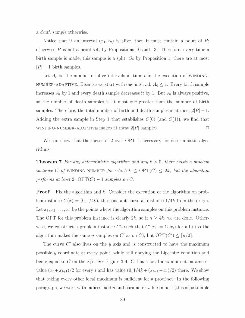
algorithm makes the same n samples on C ′ as on C), but OPT(C ′) ≤ ⌈n/2⌉.The curve C ′ also lives on the y axis and is constructed to have the maximum
possible y coordinate at every point, while still obeying the Lipschitz condition and
being equal to C on the xi’s. See Figure 3-4. C ′ has a local maximum at parameter
value (xi + xi+1)/2 for every i and has value (0, 1/4k + (xi+1−xi)/2) there. We show
that taking every other local maximum is sufficient for a proof set. In the following
paragraph, we work with indices mod n and parameter values mod 1 (this is justifiable
39
x x0 1 0 1
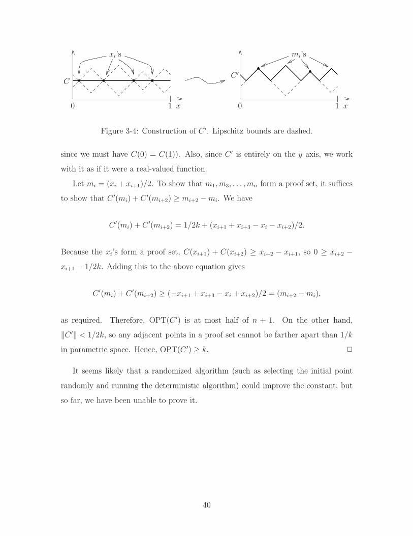
CC ′
xi’s mi’s
Figure 3-4: Construction of C ′. Lipschitz bounds are dashed.
since we must have C(0) = C(1)). Also, since C ′ is entirely on the y axis, we work
with it as if it were a real-valued function.
Let mi = (xi + xi+1)/2. To show that m1, m3, . . . , mn form a proof set, it suffices
to show that C ′(mi) + C ′(mi+2) ≥ mi+2 −mi. We have
C ′(mi) + C ′(mi+2) = 1/2k + (xi+1 + xi+3 − xi − xi+2)/2.
Because the xi’s form a proof set, C(xi+1) + C(xi+2) ≥ xi+2 − xi+1, so 0 ≥ xi+2 −xi+1 − 1/2k. Adding this to the above equation gives
C ′(mi) + C ′(mi+2) ≥ (−xi+1 + xi+3 − xi + xi+2)/2 = (mi+2 −mi),
as required. Therefore, OPT(C ′) is at most half of n + 1. On the other hand,
‖C ′‖ < 1/2k, so any adjacent points in a proof set cannot be farther apart than 1/k
in parametric space. Hence, OPT(C ′) ≥ k. 2
It seems likely that a randomized algorithm (such as selecting the initial point
randomly and running the deterministic algorithm) could improve the constant, but
so far, we have been unable to prove it.
40

Chapter 4
Noisy Samples
4.1 Noisy Approximation Problem
So far we have assumed that sampling f always returns a precise value. Now we
investigate what happens if the samples an algorithm makes are corrupted by noise.
For simplicity, we assume that the noise is normally distributed, has a known variance
σ2, and that all samples are independent. The performance of algorithms, including
OPT, is now measured as the expected number of samples performed on a problem
instance.
Due to the noise, it is unavoidable that some executions of the algorithm will be
completely wrong. A natural desired property is that the algorithm should be (ǫ, δ)-
accurate. This means that the probability of the output error being greater than ǫ
should be less than δ. In other words, the user specifies the desired accuracy and
how often the algorithm is allowed to fail to achieve this accuracy. Note that the
probability of failure is taken over the executions of the algorithm on a particular
problem instance and no prior distribution is assumed over problem instances.
Formally, the problem is defined as follows:
41
Problem noisy-lipschitz-approx:
Given: (f, σ, ǫ, δ) where f : [0, 1]→ R, 0 < σ, 0 < ǫ < 1/2, 0 < δ < 1/12
Such that: For x1, x2 ∈ [0, 1], |f(x2)− f(x1)| ≤ |x2 − x1|
and sampling at x returns a sample from N(f(x), σ2)
Compute: f : [0, 1]→ R such that for all x ∈ [0, 1], |f(x)− f(x)| ≤ ǫ
The output should be correct with probability at least 1− δ.
Notice that we don’t require the output function to be Lipschitz or even continu-
ous. Moreover, our algorithm potentially outputs a discontinuous function. As shown
at the end of the proof of Proposition 17, this is not a serious limitation.
For this problem, there is no distinction between deterministic and randomized
algorithms because a deterministic algorithm may obtain random numbers simply by
sampling the function, while δ allows a probability of failure.
In order to carry out an adaptive analysis of an algorithm for noisy-lipschitz-
approx, we need to compare its execution to that of the best possible algorithm
for the problem. However, because now an algorithm is allowed to fail with a cer-
tain probability, it is more difficult to characterize OPT. In order to get around this
difficulty, we compare the algorithm’s performance to NOPT, which we define to be
the number of samples performed by the best possible algorithm for the correspond-
ing noiseless instance. We then show that NOPT(f, ǫ) is asymptotically related to
OPT(f, σ, ǫ, δ).
We start by proving an additional property of NOPT, which we didn’t need in
Section 2.2, but which we need here. We show that decreasing ǫ does not increase
NOPT too much:
Proposition 14 NOPT(f, ǫ/2) ≤ 2 · NOPT(f, ǫ) + 1
Proof: We show that given a set of n samples xi that satisfies the conditions of
Corollary 1 for f and ǫ, there is a set of 2n+1 samples that satisfies these conditions for
f and ǫ/2. First note that sampling at ǫ/2 and 1−ǫ/2 satisfies the “end” conditions at
42
a cost of 2 additional samples. Now for all i with 1 ≤ i ≤ n−1, we show we can insert
an additional sample x between xi and xi+1 so that L(xi, x) ≤ ǫ and L(x, xi+1) ≤ ǫ.
This will result in n − 1 additional samples, for a total of n + 2 + n − 1 = 2n + 1
samples.
Fix a particular i. Let a = L(xi, xi+1). We know that a ≤ 2ǫ. Suppose that
f(xi+1) ≥ f(xi) (the other case is symmetric) and consider the function
g(x) = f(xi) + (x− xi)− a/2 = f(xi+1)− (xi+1 − x) + a/2
Clearly, f(xi) ≥ g(xi) and f(xi+1) ≤ g(xi+1). Because g is continuous and Lipschitz
functions are continuous, by the intermediate value theorem, there is an x ∈ [xi, xi+1]
for which f(x) = g(x). This will be our new sample—we show L(xi, x) ≤ ǫ:
L(xi, x) = (x− xi)− |f(x)− f(xi)| =
= (x− xi)− |g(x)− f(xi)| =
= (x− xi)− |f(xi) + (x− xi)− a/2− f(xi)| =
= (x− xi)− |(x− xi)− a/2| ≤ a/2 ≤ ǫ.
Similarly, we can show that L(x, xi+1) ≤ ǫ. 2
4.2 Sampling the Normal Distribution
To solve the noisy approximation problem, we use an (ǫ, δ)-accurate algorithm for
estimating the mean of a normal distribution as a building block. We start by con-
sidering the mean of a fixed number of samples as the estimator.
Proposition 15 Consider the normal distribution N(µ, σ2) and let G(σ, ǫ, δ) be the
minimum number of samples from N(µ, σ2) necessary for the sample mean to be an
(ǫ, δ)-accurate estimate of µ (with δ < 1/3). Then G(σ, ǫ, δ) = Θ(σ2 log(1/δ)ǫ2
).
Proof: Assume without loss of generality that µ = 0. Because the normal dis-
tribution is symmetric, the probability that the sample mean is off by more than
43
ǫ is exactly twice the probability that it is greater than ǫ. The sample mean of n
samples is distributed as N(0, σ2/n). Thus, we want to determine the minimum n
such that if µ is a sample from N(0, σ2/n), then Pr[µ > ǫ] < δ/2. Equivalently, we
need to have Pr[cǫ−1µ > c] < δ/2. Let c =√
nǫ/σ. Note that cǫ−1µ is distributed
as N(0, c2σ2ǫ−2/n) = N(0, 1). Therefore, we need to show that if c is the smallest
number such that the probability that a sample from N(0, 1) is greater than c is
smaller than δ/2, then c = Θ(√
log(1/δ)).
The probability density function of N(0, 1) is e−x2/2/√
2π. We need∫∞
ce−x2/2√
2πdx <
δ/2. Equivalently, we need∫∞
c/√
2e−y2
dy < δ√
π/4. It is well known (see [AS72]) that
e−c2/2
c/√
2 +√
c2/2 + 2≤∫ ∞
c/√
2
e−y2
dy ≤ e−c2/2
c/√
2 +√
c2/2 + 4/π.
From the right inequality, if c >√
2 log(1/δ), then∫∞
c/√
2e−y2
dy < δ√
π/4. On the
other hand, from the left inequality, if c <√
log(1/δ)/5, we have
∫ ∞
c/√
2
e−y2
dy ≥ e−c2/2
c/√
2 +√
c2/2 + 2≥ δ1/10
2√
log(1/δ)/10 + 2≥ δ1/10
√
2/5δ + 38/5=
= δ√
π/4
√
δ1/5/(δ2π/4)
2/5δ + 38/5= δ√
π/4
√
10
π(δ4/5 + 19δ9/5).
So∫∞
c/√
2e−y2
dy > δ√
π/4 if δ ≤ 1/3. 2
Thus, an algorithm to find an (ǫ, δ)-accurate value of f at x is to sample G(σ, ǫ, δ)
times and return the average. The following proposition shows that it is impossible
to do better and will be useful in proving lower bounds on OPT. Unfortunately, the
proof is quite messy and we have not been able to find a cleaner one.
Proposition 16 Any algorithm that distinguishes between N(0, σ2) and N(ǫ, σ2),
with error probability at most δ < 1/12, uses Ω(G(σ, ǫ, δ)) samples in expectation
when the true distribution is N(0, σ2).
44
Proof: In general, at every step, the algorithm may choose to either sample the
distribution, or output an answer. Call an algorithm symmetric if it outputs 0 after
samples x1, . . . , xk whenever it outputs ǫ after ǫ− x1, . . . , ǫ− xk. We first show that
for every algorithm, there is a symmetric algorithm whose performance is within a
constant factor.
We start by taking the algorithm that distinguishes between N(0, σ2) and N(ǫ, σ2)
with error probability at most δ and transforming it by amplification (this is where
we lose the constant) to have error at most δ/2. We now transform it to be symmetric
by simultaneously simulating two “copies” of the algorithm. Each new sample x is fed
unchanged to the first copy, and as ǫ−x to the second copy. If the first copy outputs
a (and the second copy either outputs ǫ − a or needs more samples), the algorithm
stops and outputs a. If the second copy outputs a, the algorithm stops and outputs
ǫ − a. If both copies output a, the algorithm outputs 0 or ǫ with equal probability.
This algorithm errs with probability at most δ because by the union bound, with
probability δ, neither copy makes a mistake. The expected number of samples this
algorithm performs is no larger than that of either copy, since it terminates whenever
either copy terminates.
Now let k be the expected number of samples the symmetric algorithm makes.
By Markov’s inequality, the probability that the algorithm requires more than 4k
samples is less than 1/4. So we may relax the conditions of the algorithm to turn it
into one that does the following: it first performs 4k samples, then with probability
3/4 it must output an answer; with probability 1/4 it is allowed to ask an oracle that
always gives the correct answer. If the algorithm decides to output the answer, it can
make errors with probability at most 4δ/3. Let ERR be the event that the algorithm
outputs incorrectly and STEPS4k be the event that it outputs without asking the
oracle. Then:
Pr[ERR] = Pr[ERR ∧ STEPS4k] = Pr[STEPS4k] · Pr[ERR | STEPS4k] ≤ δ.
45
Let the 4k samples the algorithm makes be x1, . . . , x4k and let x = (x1, . . . , x4k)
be the corresponding point in R4k. Let f0(x): R4k → [0, 1] be the probability that
the algorithm outputs 0 on that input. Because the algorithm is symmetric, it is
completely characterized by f0. However, for notational convenience, let fǫ(x) be
the probability that the algorithm outputs ǫ, so fǫ(x) = f0(ǫ − x), where ǫ − x is
shorthand for (ǫ− x1, . . . , ǫ− xn). Let
PDF a,σ =e−(x−a)2/(2σ2)
σ√
2π
be the probability density function of a single sample. Then the PDF of x is
Pa(x) =
4k∏
i=1
PDFa,σ(xi) =e
−P4k
i=1(xi−a)2
2σ2
(σ√
2π)4k= PDFa
√4k,σ
(
x · 1/√
4k)
· e−
‚
‚
‚
‚
x−x(x·1/√
4k)‖x‖
‚
‚
‚
‚
2
2σ2
(σ√
2π)4k−1
where a is the mean of the true distribution and 1 is the vector (1, . . . , 1) so 1/√
4k
is a unit vector. In order for the algorithm to be correct, f0 and fǫ must satisfy these
conditions:
∫
R4k
fǫ(x)P0(x)dx ≤ δ and
∫
R4k
(fǫ(x) + f0(x))P0(x)dx ≥ 3/4.
Now let A = x ∈ R4k |∑4k
i=1 xi > 2kǫ. Note that for all x ∈ A, P0(x) < P0(ǫ− x).
Also, clearly if x ∈ A, then ǫ − x 6∈ A. Now let S = x ∈ A | f0(x) > 0. If S
is non-empty, we can lower the probability of failure (i.e., reduce the first integral
without changing the second) by letting
f ′0(x) =
0, if x ∈ S,
f0(x) + fǫ(x), if ǫ− x ∈ S,
f0(x), otherwise.
Therefore, we may assume that f0 is 0 on A (in other words, the algorithm never
outputs 0 when the mean of the samples is closer to ǫ).
46
Now we split A: let B = x ∈ R4k | ∑4k
i=1 xi > 4kǫ and C = x ∈ R4k | 2kǫ <
∑4ki=1 xi ≤ 4kǫ. We want to show that we can transform the algorithm to one with
fǫ = 1 on B that is correct with probability 1−δ and asks the oracle with probability at
most 1/4+δ. Suppose that∫
B(1−fǫ(x))Pǫ(x)dx = 1/2−
∫
Bfǫ(x)Pǫ(x)dx = c > 0. We
know that∫
Afǫ(x)Pǫ(x)dx ≥ 3/4− δ ≥ 1/2 if δ ≤ 1/4. Therefore,
∫
Cfǫ(x)Pǫ(x) ≥ c.
Let D ⊂ C be such that∫
Dfǫ(x)Pǫ(x) = c. Now we can transform the algorithm
by letting f ′ǫ = 1 on B and f ′
ǫ = 0 on D and f ′ǫ = fǫ everywhere else. The integral
∫
Afǫ(x)Pǫ(x)dx is unchanged and the integral
∫
R4k−Af0(x)Pǫ(x)dx was at most δ to
begin with, so the transformed algorithm outputs after 4k samples with probability
at least 3/4− δ. We now show that the transformed algorithm errs with probability
no more than δ. The error probability of the new algorithm is∫
Af ′
ǫ(x)P0(x)dx. This
is equal to
∫
A
fǫ(x)P0(x)dx +
∫
B
(1− fǫ(x))P0(x)dx−∫
D
fǫ(x)P0(x)dx.
Thus, we need to show that∫
B(1 − fǫ(x))P0(x)dx ≤
∫
Dfǫ(x)P0(x)dx. Now let
g1(x) = (1− fǫ(x))Pǫ(x) and let g2(x) = fǫ(x)Pǫ(x). By construction,∫
Bg1(x)dx =
∫
Dg2(x)dx. Notice that
P0(x)/Pǫ(x) =PDF0,σ
(
x · 1/√
4k)
PDFǫ√
4k,σ
(
x · 1/√
4k) =
e−(x·1/√
4k)2/(2σ2)
e−(x·1/√
4k−ǫ√
4k)2/(2σ2)= e
„
−ǫ24k−2ǫ(x·1)
2σ2
«
and the rightmost expression is a decreasing function of x·1. Because x·1 is greater ev-
erywhere on B than on D, we have∫
Bg1(x)P0(x)/Pǫ(x)dx ≤
∫
Dg2(x)P0(x)/Pǫ(x)dx,
as necessary. It is easy to modify the transformed algorithm into one that uses the
oracle with probability at most 1/4, but has error probability 2δ. This algorithm has
fǫ = 1 on B. In other words, if the mean of the 4k samples is at least ǫ, it outputs
ǫ. Now consider the probability that the mean of 4k samples from N(0, σ) is at least
ǫ (because in this case the algorithm makes a mistake). If 4k ≤ G(σ, ǫ, 4δ), this
probability is at least 2δ, so the algorithm cannot work unless k = Ω(G(σ, ǫ, δ)). 2
47
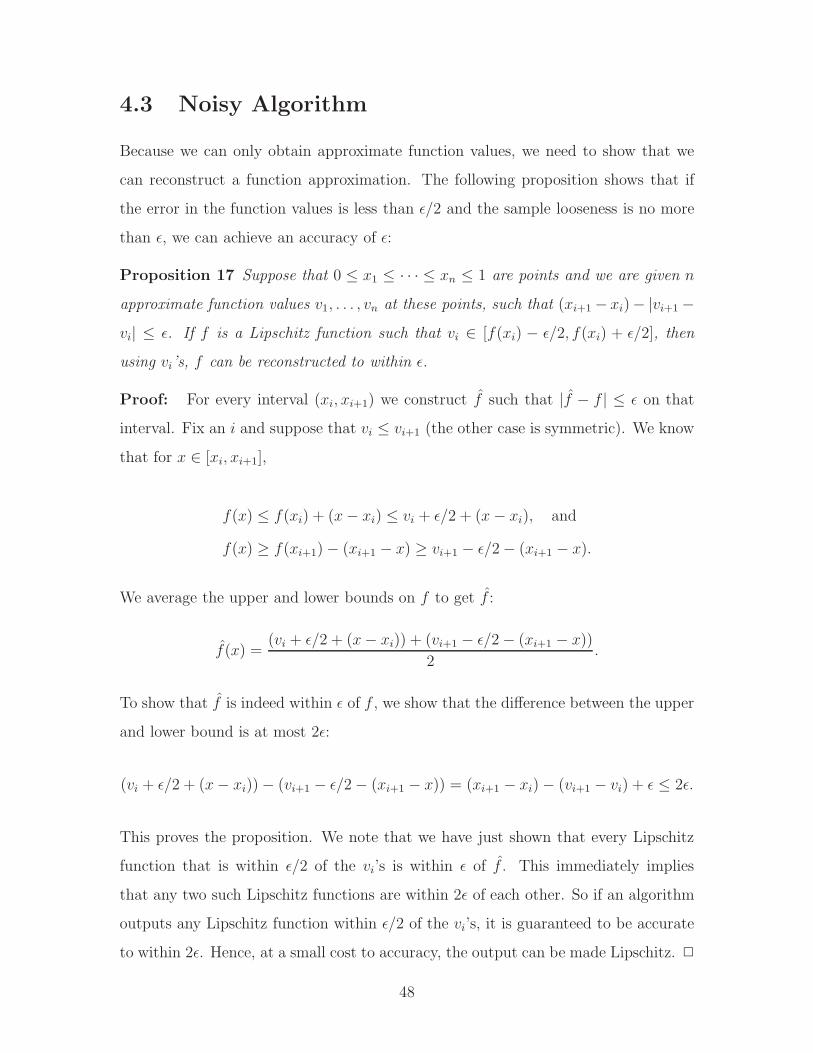
4.3 Noisy Algorithm
Because we can only obtain approximate function values, we need to show that we
can reconstruct a function approximation. The following proposition shows that if
the error in the function values is less than ǫ/2 and the sample looseness is no more
than ǫ, we can achieve an accuracy of ǫ:
Proposition 17 Suppose that 0 ≤ x1 ≤ · · · ≤ xn ≤ 1 are points and we are given n
approximate function values v1, . . . , vn at these points, such that (xi+1− xi)− |vi+1−vi| ≤ ǫ. If f is a Lipschitz function such that vi ∈ [f(xi) − ǫ/2, f(xi) + ǫ/2], then
using vi’s, f can be reconstructed to within ǫ.
Proof: For every interval (xi, xi+1) we construct f such that |f − f | ≤ ǫ on that
interval. Fix an i and suppose that vi ≤ vi+1 (the other case is symmetric). We know
that for x ∈ [xi, xi+1],
f(x) ≤ f(xi) + (x− xi) ≤ vi + ǫ/2 + (x− xi), and
f(x) ≥ f(xi+1)− (xi+1 − x) ≥ vi+1 − ǫ/2− (xi+1 − x).
We average the upper and lower bounds on f to get f :
f(x) =(vi + ǫ/2 + (x− xi)) + (vi+1 − ǫ/2− (xi+1 − x))
2.
To show that f is indeed within ǫ of f , we show that the difference between the upper
and lower bound is at most 2ǫ:
(vi + ǫ/2 + (x− xi))− (vi+1 − ǫ/2− (xi+1 − x)) = (xi+1 − xi)− (vi+1 − vi) + ǫ ≤ 2ǫ.
This proves the proposition. We note that we have just shown that every Lipschitz
function that is within ǫ/2 of the vi’s is within ǫ of f . This immediately implies
that any two such Lipschitz functions are within 2ǫ of each other. So if an algorithm
outputs any Lipschitz function within ǫ/2 of the vi’s, it is guaranteed to be accurate
to within 2ǫ. Hence, at a small cost to accuracy, the output can be made Lipschitz. 2
48
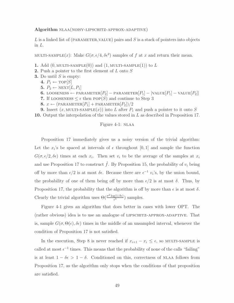
Algorithm nlaa(noisy-lipschitz-approx-adaptive)
L is a linked list of (parameter,value) pairs and S is a stack of pointers into objectsin L.
multi-sample(x): Make G(σ, ǫ/4, δǫ2) samples of f at x and return their mean.
1. Add (0,multi-sample(0)) and (1,multi-sample(1)) to L2. Push a pointer to the first element of L onto S3. Do until S is empty:
4. P1 ← top[S]5. P2 ← next[L, P1]6. looseness← parameter[P2]− parameter[P1]− |value[P1]− value[P2]|7. If looseness ≤ ǫ then pop(S) and continue to Step 38. x← (parameter[P1] + parameter[P2])/29. Insert (x,multi-sample(x)) into L after P1 and push a pointer to it onto S
10. Output the interpolation of the values stored in L as described in Proposition 17.
Figure 4-1: nlaa
Proposition 17 immediately gives us a noisy version of the trivial algorithm:
Let the xi’s be spaced at intervals of ǫ throughout [0, 1] and sample the function
G(σ, ǫ/2, δǫ) times at each xi. Then set vi to be the average of the samples at xi
and use Proposition 17 to construct f . By Proposition 15, the probability of vi being
off by more than ǫ/2 is at most δǫ. Because there are ǫ−1 vi’s, by the union bound,
the probability of one of them being off by more than ǫ/2 is at most δ. Thus, by
Proposition 17, the probability that the algorithm is off by more than ǫ is at most δ.
Clearly the trivial algorithm uses Θ(σ2 log(1/δǫ)ǫ3
) samples.
Figure 4-1 gives an algorithm that does better in cases with lower OPT. The
(rather obvious) idea is to use an analogue of lipschitz-approx-adaptive. That
is, sample G(σ, Θ(ǫ), δǫ) times in the middle of an unsampled interval, whenever the
condition of Proposition 17 is not satisfied.
In the execution, Step 8 is never reached if xi+1 − xi ≤ ǫ, so multi-sample is
called at most ǫ−1 times. This means that the probability of none of the calls “failing”
is at least 1 − δǫ > 1 − δ. Conditioned on this, correctness of nlaa follows from
Proposition 17, as the algorithm only stops when the conditions of that proposition
are satisfied.
49
We now turn to analyzing nlaa’s performance. It makes Θ(G(σ, ǫ, δǫ2)ǫ−1) sam-
ples in the worst case (for instance, in correct executions when f is constant). We
would like to analyze its performance relative to OPT, but that seems extremely dif-
ficult. Instead, we analyze its performance relative to NOPT and then in the next
sections show that OPT(f, σ, ǫ, δ) = Θ(G(σ, ǫ, δ)NOPT(f, ǫ)).
Theorem 8 nlaa performs O(G(σ, ǫ, δǫ)·NOPT(f, ǫ) log(ǫ−1/NOPT(f, ǫ))) samples
on the problem instance (f, σ, ǫ, δ).
Proof: To analyze the algorithm’s performance relative to NOPT, we compare its
execution to that of lipschitz-approx-adaptive on (f, ǫ/4), which, by Theorem 1,
performs O(NOPT(f, ǫ/4) log(4ǫ−1/NOPT(f, ǫ/4))) samples.
First, suppose that no call to multi-sample fails—that is, each call returns a
value within ǫ/4 of f(x). We show that nlaa makes at most as many calls to
multi-sample as the noiseless algorithm, with its error tolerance set to ǫ/4, makes
samples. Because both nlaa and lipschitz-approx-adaptive always sample in
the middle of an unsampled interval whose length is greater than Θ(ǫ), an execution
of each algorithm corresponds to a subtree of a complete binary tree of Θ(ǫ−1) nodes.
The root of this tree is the entire interval [0, 1], the next level consists of the intervals
[0, 1/2] and [1/2, 1], and so on. A node is in the subtree if the corresponding interval
appeared between points in L during the execution of the algorithm. Therefore, the
number of calls to multi-sample or samples (in the noisy and noiseless setting,
respectively) is equal to the size of the subtree.
We show that the subtree corresponding to the noisy algorithm (in the case of no
failures) is no bigger than the subtree corresponding to the noiseless algorithm. To
obtain the noiseless algorithm, Step 7 is replaced by “If L(xi, xi+1) ≤ ǫ/2, continue”
(see Step 6 in lipschitz-approx-adaptive). But because |f(x)− f(x)| ≤ ǫ/4, we
have |f(xi)− f(xi+1)| ≥ |f(xi)− f(xi+1)| − ǫ/2, so
(xi+1−xi)−|f(xi+1)− f (xi)| ≤ (xi+1−xi)−|f(xi+1)−f(xi)|+ǫ/2 = L(xi, xi+1)+ǫ/2.
50

Therefore, if the children of a node are not included in the noiseless subtree, they
are also not included in the noisy subtree. So nlaa performs O(NOPT(f, ǫ/4) ·log(4ǫ−1/NOPT(f, ǫ/4))) calls to multi-sample. By two applications of Proposition
14, this is the claimed bound.
The probability of multi-sample failing at least once during an execution is at
most δǫ, and the nlaa makes fewer than ǫ−1 calls to multi-sample, even in case of
failure, so the expected number of extra calls to multi-sample due to failure is at
most δ, which is smaller than 1. 2
4.4 Bounds on OPT in Terms of NOPT
For the purposes of comparing algorithms to OPT once their performance is expressed
in terms of NOPT, it is important to have a lower bound on OPT in terms of NOPT.
We show the following such bound:
Theorem 9 OPT(f, σ, ǫ, δ) = Ω(G(σ, ǫ, δ) · NOPT(f, ǫ))
Proof: We show that every algorithm for the noisy problem is forced to solve at least
NOPT(f, 2ǫ)/2 independent instances of the distinguishing-between-two-Gaussians
problem, which gives the desired bound.
First of all, let n = NOPT(f, 2ǫ) and let xi for 1 ≤ i ≤ n be a smallest proof set for
the noiseless problem instance. So L(xi, xi+1) ≤ 4ǫ < L(xi, xi+2). As we are proving
a lower bound on the noisy algorithm, we are allowed to give the noisy algorithm free
extra information to simplify the argument. So suppose we give the noisy algorithm
the exact function values at all xi’s where i is odd. With this information, if i is
odd, sampling in an interval [xi, xi+2] gives the algorithm no information about the
behavior of f in any other interval (because both f(xi) and f(xi+2) are already known
exactly).
Now consider a particular odd i and the interval [xi, xi+2]. Because L(xi, xi+2) >
4ǫ, by Proposition 5(2), there is a point x ∈ [xi, xi+2] and a Lipschitz function f ′
equal to f at xi and xi+2 such that |f ′(x) − f(x)| > 2ǫ. By choosing f ′ correctly,
51
we can also guarantee that x is the point where |f ′ − f | is maximized and that
|f ′(x) − f(x)| < 3ǫ. Extend f ′ to [0, 1] by setting f ′ = f everywhere except on
[xi, xi+2]. Now any function f that approximates f within ǫ cannot approximate f ′
within ǫ, at least at x. So the best possible algorithm has to at least distinguish f from
f ′ (which only differ on [xi, xi+2]). Because x is the point where f and f ′ differ most,
by a simple reduction, distinguishing f from f ′ is at least as hard as distinguishing
f(x) from f ′(x), which differ by no more than 3ǫ. Thus, on every interval, the best
possible algorithm must use Ω(G(σ, 3ǫ, δ)) samples in expectation to distinguish f(x)
from f ′(x), by Proposition 16. Because there are n/2 intervals, the total number of
samples necessary is Ω(n ·G(σ, ǫ, δ)). 2
Together, Theorems 8 and 9 show that the number of samples nlaa performs is
at most
O
(
OPT(f, σ, ǫ, δ) · (log(1/δ) + log(1/ǫ)) log(1/ǫ)
log(1/δ)
)
= O(OPT(f, σ, ǫ, δ) log2(1/ǫ)).
We now turn to proving an upper bound on OPT in terms of NOPT in order to
show the tightness of Theorem 9. It is easy to prove the upper bound
OPT(f, σ, ǫ, δ) = O
(
G
(
σ, ǫ,δ
NOPT(f, ǫ)
)
NOPT(f, ǫ)
)
.
Tightening this to OPT(f, σ, ǫ, δ) = O(G(σ, ǫ, δ) · NOPT(f, ǫ)) is a bit tricky. The
idea is to take advantage of the fact that the best possible algorithm is optimized
for a particular instance and only sample with higher accuracy in regions where the
input function doesn’t look like the one for which the algorithm is optimized.
First, we prove a proposition related to Proposition 17:
Proposition 18 Let 0 ≤ x1 ≤ · · · ≤ xn ≤ 1 be a proof set for (f, ǫ/4). Suppose
f ′ is a Lipschitz function such that |f ′(xi) − f(xi)| ≤ ǫ/2 for all i. Then for all x,
|f ′(x)− f(x)| ≤ ǫ.
Proof: If x < x1, then because x1 ≤ ǫ/4, we have f(x) ∈ [f(x1)− ǫ/4, f(x1) + ǫ/4],
and f ′(x) ∈ [f ′(x1)− ǫ/4, f ′(x1) + ǫ/4] ⊂ [f(x1)− 3ǫ/4, f(x1) + 3ǫ/4]. The maximum
52
possible difference between points in these two intervals is ǫ. Similarly for x > xn.
Otherwise, for some i, x ∈ [xi, xi+1]. Suppose that f(xi) ≤ f(xi+1) (the other case
is symmetric). Then by the Lipschitz condition, f(x) ∈ [f(xi+1)− (xi+1− x), f(xi) +
(x − xi)] and f ′(x) ∈ [f ′(xi+1) − (xi+1 − x), f ′(xi) + (x − xi)] ⊂ [f(xi+1) − (xi+1 −x) − ǫ/2, f(xi) + (x − xi) + ǫ/2]. But Lf (xi, xi+1) ≤ ǫ/2, so f(x) is contained in an
interval of the form [a− ǫ/4, a+ ǫ/4] and f ′(x) is contained in an interval of the form
[a− 3ǫ/4, a + 3ǫ/4] (the a’s are the same), which proves that the maximum possible
difference between f(x) and f ′(x) is ǫ. 2
Theorem 10 OPT(f, σ, ǫ, δ) = O(G(σ, ǫ, δ) ·NOPT(f, ǫ))
Proof: Let xi’s be a smallest noiseless proof set of size n for (f, ǫ/4). Then
Lf (xi, xi+1) ≤ ǫ/2 and n = O(NOPT(f, ǫ)) by Proposition 14. Let f be the function
the algorithm is optimized for and let f ′ be the function fed to it. The algorithm is
as follows:
1. Make G(σ, ǫ/4, δ/4) samples of f ′ at each xi and let vi’s be the sample means.2. Starting with k = 3, do while 2−k > ǫ3/4 (and increment k on each loop):
3. Mark all i’s for which |vi − f(xi)| > ǫ/4. If none marked, output f .4. Make G(σ, ǫ/4, δ/2k) samples of f ′ at each marked xi and let vi’s be the means.
5. Output the result of running the “trivial” algorithm passing it δ/2 instead of δ.
To prove correctness, we first consider the case f ′ = f . Note that the loop
completes only if there is a vi marked in each round. The probability of a particular
vi being marked in all rounds (once a vi is unmarked, it stays unmarked) is at most
the probability of it being marked in the last round, which is at most δǫ3. Thus,
the probability of any vi staying marked is at most δǫ2 so with probability at least
1− δǫ2 > 1− δ, f is correctly output.
If f ′ 6= f , we only care about the case when f is not within ǫ of f ′ (otherwise, it is
fine if f is output). In this case, by the contrapositive of Proposition 18, for some xi,
|f ′(xi)−f(xi)| ≥ ǫ/2. This means that the probability of that xi getting unmarked in
round k is at most δ/2k. By the union bound, the probability of it getting unmarked
at all is at most δ/2. Thus, with probability at least 1 − δ/2 the algorithm reaches
53
Step 5 (and conditioned on that, the output is correct with probability 1−δ/2). This
proves that the algorithm is correct with probability at least 1− δ, as necessary.
We now analyze expected performance for f ′ = f . The expected number of
samples made at xi in Steps 1–4 is at most (roughly)
G(σ, ǫ/4, δ/4) +δ
4G(σ, ǫ/4, δ/8) +
δ
8G(σ, ǫ/4, δ/16) + · · · < 2G(σ, ǫ/4, δ/4).
Thus the total expected number of samples in Steps 1–4 is O(nG(σ, ǫ, δ)), as claimed.
Step 5 is reached with probability less than δǫ2 and makes ǫ−1G(σ, ǫ, δǫ) samples.
Thus, the expected number of samples in Step 5 is O( δ(log δ−1+log ǫ−1)ǫ
), which is small
compared to G(σ, ǫ, δ). 2
54
Chapter 5
Functions Whose Domain is in Rd
5.1 Higher Dimensional Domains
When d > 1, devising and analyzing adaptive algorithms becomes much more difficult.
There are several reasons for this difficulty:
(1) If the domain is [0, 1] and an algorithm has sampled 0 = x1 < x2 < · · · < xn =
1, and x ∈ [xi, xi+1], the Lipschitz condition for xi and x is a stronger constraint on
f(x) than the condition for xj and x if i ≥ j. No obvious analogue of this statement
is true when the domain is higher-dimensional. The implication is that OPT may
use a single well-placed sample to tighten bounds on the function very far away, but
finding this well-placed sample will be difficult for the algorithm.
(2) When d = 1, every connected domain is an interval. This is not true for d > 1.
Assuming that the algorithm knows the shape of the domain a priori is reasonable
for lower bounds, but not for algorithms. Making the shape of the domain part of
the input to the algorithm presents its own difficulties, such as representation, as
well analyzing the amount of time the algorithm spends doing computations with the
shape.
(3) When d = 1, after a finite number of samples, Lipschitz bounds are piecewise-
linear with few pieces (see, e.g., Figure 2-2). However, when d > 1, the region deter-
mined by the Lipschitz condition is an intersection of cones and has a combinatorial
structure analogous to that of a Voronoi diagram. Computations that algorithms
55
may need to perform on this structure may have very high cost, even compared to
the sampling cost.
The second and third reasons point to potential inadequacies of computation
models, but the first is fundamental to the problem.
5.2 Lower Bounds for Function Minimization
We present a lower bound that shows that when the domain is a closed unit ball Bd,
good adaptive algorithms do not exist for the function minimization problem.
Problem lipschitz-ball-minimize:
Given: (f, ǫ) where f : Bd → R, 0 < ǫ < 1/2
Such that: For x1, x2 ∈ Bd, |f(x2)− f(x1)| ≤ ‖x2 − x1‖
Compute: x such that for all y ∈ Bd, f(x) ≤ f(y) + ǫ
Theorem 11 For any ǫ with 1/2 > ǫ > 0 and for any deterministic algorithm, there
exists function g such that OPT(g, ǫ) = 2, but the algorithm makes Ω(ǫ1−d) samples.
Proof: Consider the “hat” function f(x) = max(1 − ‖x‖, 2ǫ). Let B1, B2, . . . , Bn
be a tight packing of balls of radius 3ǫ/2 with centers on Sd, the boundary of B
d.
The number of these balls is Θ(ǫ1−d), where the constant in Θ may depend on d. Let
c1, . . . , cn be the centers of the balls. Let gi: Bd → R be defined as
gi(x) =
ǫ/2 + ‖x− ci‖, for x ∈ Bi,
f(x), otherwise.
See Figure 5-1. Because Bi is contained in the region where f = 2ǫ, all gi’s are
Lipschitz. The only solutions to the minimization problem for (gi, ǫ) are on Bi,
because gi(ci) = ǫ/2, but everywhere not on Bi, gi is at least 2ǫ. For each gi, sampling
at 0 and ci is sufficient to prove that ci is a solution because by the Lipschitz condition,
|gi(x)− 1| < ‖x‖, which implies that gi(x) > 0. Therefore, OPT(gi, ǫ) = 2.
Now sampling gi anywhere except at Bi gives no information about which of the
balls contains the minimum (beyond that it is not the ball, if any, that contains the
56

Figure 5-1: Illustration of gi for Theorem 11 with d = 2. Other Bj’s are shown dotted.
sample). Therefore, an algorithm is forced to do a linear search over the balls, which
gives the desired result. 2
This lower bound heavily relies on the fact that the domain is a ball. The gener-
alization of this bound to other domain shapes is the following:
Proposition 19 Let f have domain S. Let (b1, r1), . . . , (bm, rm) be balls centered at
bi ∈ S with radii ri such that for any point x ∈ S, there is an i for which ‖x− bi‖ ≤ri + 2ǫ. Suppose n non-intersecting balls of radius R > ǫ with centers in S can be
packed between the m balls. Then there is a family of n problem instances, such that
OPT ≤ m + 1 for each member of the family, but any algorithm uses Ω(n) samples
for some problem instance.
Proof: Assume that none of the m balls is contained within another one (otherwise,
it may be removed without violating the premise). Let f(x) = max(maxi(2ǫ + ri −‖x−bi‖), 2ǫ). Clearly, f is Lipschitz because it is the maximum of Lipschitz functions.
Note that f(bi) = 2ǫ + ri because none of the balls contain each other. We now show
that sampling at the m bi’s proves that f ≥ 0 everywhere on S. Given x ∈ S, pick an
i such that ‖x− bi‖ ≤ ri + 2ǫ. By the Lipschitz condition, f(x) ≥ f(bi)− ri− 2ǫ = 0.
Let the n packed balls be B1, . . . , Bn with centers at c1, . . . , cn. Now, as in the
proof of Theorem 11, let each member of the problem instance family be defined as
57
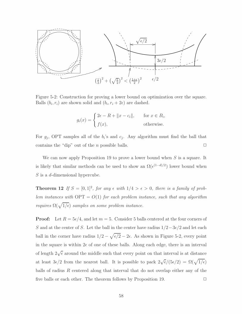
3ǫ/2
√
ǫ/2
ǫ/2(
12
)2+(√
ǫ2
)2<(
1+ǫ2
)2
Figure 5-2: Construction for proving a lower bound on optimization over the square.Balls (bi, ri) are shown solid and (bi, ri + 2ǫ) are dashed.
gi(x) =
2ǫ− R + ‖x− ci‖, for x ∈ Bi,
f(x), otherwise.
For gj, OPT samples all of the bi’s and cj. Any algorithm must find the ball that
contains the “dip” out of the n possible balls. 2
We can now apply Proposition 19 to prove a lower bound when S is a square. It
is likely that similar methods can be used to show an Ω(ǫ(1−d)/2) lower bound when
S is a d-dimensional hypercube.
Theorem 12 If S = [0, 1]2, for any ǫ with 1/4 > ǫ > 0, there is a family of prob-
lem instances with OPT = O(1) for each problem instance, such that any algorithm
requires Ω(√
1/ǫ) samples on some problem instance.
Proof: Let R = 5ǫ/4, and let m = 5. Consider 5 balls centered at the four corners of
S and at the center of S. Let the ball in the center have radius 1/2−3ǫ/2 and let each
ball in the corner have radius 1/2−√
ǫ/2− 2ǫ. As shown in Figure 5-2, every point
in the square is within 2ǫ of one of these balls. Along each edge, there is an interval
of length 2√
ǫ around the middle such that every point on that interval is at distance
at least 3ǫ/2 from the nearest ball. It is possible to pack 2√
ǫ/(5ǫ/2) = Ω(√
1/ǫ)
balls of radius R centered along that interval that do not overlap either any of the
five balls or each other. The theorem follows by Proposition 19. 2
58
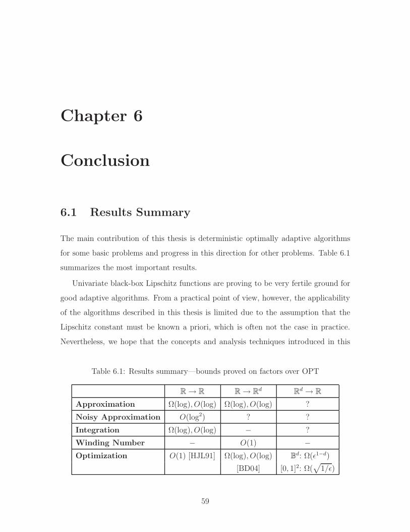
Chapter 6
Conclusion
6.1 Results Summary
The main contribution of this thesis is deterministic optimally adaptive algorithms
for some basic problems and progress in this direction for other problems. Table 6.1
summarizes the most important results.
Univariate black-box Lipschitz functions are proving to be very fertile ground for
good adaptive algorithms. From a practical point of view, however, the applicability
of the algorithms described in this thesis is limited due to the assumption that the
Lipschitz constant must be known a priori, which is often not the case in practice.
Nevertheless, we hope that the concepts and analysis techniques introduced in this
Table 6.1: Results summary—bounds proved on factors over OPT
R→ R R→ Rd
Rd → R
Approximation Ω(log), O(log) Ω(log), O(log) ?
Noisy Approximation O(log2) ? ?
Integration Ω(log), O(log) − ?
Winding Number − O(1) −Optimization O(1) [HJL91] Ω(log), O(log) B
d: Ω(ǫ1−d)
[BD04] [0, 1]2: Ω(√
1/ǫ)
59
thesis will prove useful in developing adaptive algorithms for more practical problems.
6.2 Future Research
There are many related problems left unexplored. We have shown that generalizing
adaptive optimization algorithms to higher-dimensional domains is impossible, but
perhaps integration or approximation do have good adaptive algorithms in higher di-
mensions. In particular, if Monte Carlo algorithms are allowed, integration does not
suffer from the “curse of dimensionality,” so the existence of good adaptive Monte
Carlo algorithms would be especially interesting. Even for univariate functions, adap-
tive Monte Carlo integration algorithms are significantly more powerful than adaptive
deterministic algorithms, as I plan to show in a forthcoming paper.
For the noisy approximation problem, there is a log2 gap between upper and
lower bounds, so the “adaptive complexity” of noisy approximation is open. We have
analyzed the extent to which the approximation problem becomes more difficult with
random noise, but have not considered integration or optimization with noise. Also,
we make very strong assumptions about the noise; are algorithms possible if we do
not assume that the noise components in samples are i.i.d.?
We do not know what assumptions other than the Lipschitz condition lead to
interesting adaptive algorithms. For example, we could consider functions whose nth
derivative is Lipschitz, functions that are sums or products of Lipschitz functions
(e.g., we are given several Lipschitz functions and need to compute the minimum of
their sum), or functions chosen at random according to some distribution.
60
Bibliography
[AS72] Milton Abramowitz and Irene A. Stegun, editors. Handbook of Mathemati-
cal Functions with Formulas, Graphs, and Mathematical Tables, chapter 7.
Dover, New York, 1972.
[BBD+04] Therese Biedl, Brona Brejova, Erik D. Demaine, Angele M. Hamel, Ale-
jandro Lopez-Ortiz, and Tomas Vinar. Finding hidden independent sets
in interval graphs. Theoretical Computer Science, 310(1–3):287–307, Jan-
uary 2004.
[BD04] Ilya Baran and Erik D. Demaine. Optimal adaptive algorithms for find-
ing the nearest and farthest point on a parametric black-box curve. In
Proceedings of the 20th Annual ACM Symposium on Computational Ge-
ometry, Brooklyn, NY, June 2004. To appear.
[CLRS01] Thomas H. Cormen, Charles E. Leiserson, Ronald L. Rivest, and Clifford
Stein. Introduction to Algorithms. The MIT Press, McGraw-Hill Book
Company, second edition, 2001.
[Dan71] Y.M. Danilin. Estimation of the efficiency of an absolute-minimum-
finding algorithm. USSR Computational Mathematics and Mathematical
Physics, 11:261–267, 1971.
[DLOM00] Erik D. Demaine, Alejandro Lopez-Ortiz, and J. Ian Munro. Adaptive
set intersections, unions, and differences. In Proceedings of the 11th An-
nual ACM-SIAM Symposium on Discrete Algorithms, pages 743–752, San
Francisco, California, January 2000.
[ECW92] Vladimir Estivill-Castro and Derick Wood. A survey of adaptive sorting
algorithms. ACM Computing Surveys, 24(4):441–476, December 1992.
61
[Elk04] Michael L. Elkin. A faster distributed protocol for constructing a mini-
mum spanning tree. In Proceedings of the 15th Annual ACM-SIAM Sym-
posium on Discrete Algorithms, pages 352–361, New Orleans, LA, January
2004.
[FLN03] Ronald Fagin, Amnon Lotem, and Moni Naor. Optimal aggregation al-
gorithms for middleware. Journal of Computer and System Sciences,
66(4):614–656, 2003.
[GW90] Oliver Gunther and Eugene Wong. The arc tree: an approximation
scheme to represent arbitrary curved shapes. Computer Vision, Graphics,
and Image Processing, 51:313–337, 1990.
[HJ95] Pierre Hansen and Brigitte Jaumard. Lipschitz optimization. In Reiner
Horst and Panos M. Pardalos, editors, Handbook of Global Optimization,
pages 407–494. Kluwer, 1995.
[HJL91] Pierre Hansen, Brigitte Jaumard, and Shi-Hui Lu. On the number of
iterations of piyavskii’s global optimization algorithm. Mathematics of
Operations Research, 16(2):334–350, May 1991.
[Piy72] S.A. Piyavskii. An algorithm for finding the absolute extremum of a
function. USSR Computational Mathematics and Mathematical Physics,
12:57–67, 1972.
[TWW88] J.F. Traub, G.W. Wasilkowski, and H. Wozniakowski. Information-Based
Complexity. Academic Press, New York, 1988.
[Wer02] Arthur G. Werschulz. An overview of information-based complexity. Tech-
nical Report CUCS-022-02, Computer Science Department, Columbia
University, October 2002.
[ZKS03] Z. Zabinsky, B.P. Kristinsdottir, and R.L. Smith. Optimal estimation
of univariate black-box lipschitz functions with upper and lower error
bounds. Computers and Operations Research, 30(10):1539–1553, 2003.
62
![Adaptive Impact-Driven Detection of Silent Data Corruption ...shdi/download/impact-driven-sdc.pdf · Sedov [20] Flash Hydrodynamical test code involving strong shocks and non-planar](https://img.pdfslide.us/doc/110x75/5f25d056ede4cf226f2df179/adaptive-impact-driven-detection-of-silent-data-corruption-shdidownloadimpact-driven-sdcpdf.jpg)