Embed Size (px)
Citation preview
Chapter 4 Gaussian Approximations to the Algorithms
Introduction In this chapter, we shall formally state and prove the "asymptotic normality" properties described in Chapter 3 of Part I.
Firstly we shall consider algorithms with constant step size, and in particular, the case in which the algorithm
is such that the associated continuous-time step function frY(t) converges to the solution O(t) of the mean differential equation, in the sense studied in the previous chapter:
limP{ sup IfrY(t) - O(t)1 > 7]} = 0 '1-+0 09~T
for all T > 0 and 7] > o. In order to investigate the "quality" of the approximation of frY(t) by O(t)
(or the "rate of convergence" as, -+ 0), it was suggested in Part I, that we should study the process ,-1/2(O'Y(t) - O(t)). If we multiply the fluctuations of this process by .,fY, we obtain the fluctuations of frY(t) about O(t).
This process is in general difficult to study directly, whence, often a process with a "similar distribution" for small, is substituted in its place. Chapter 3 of Part I expresses the fact that one such process is a "Gaussian diffusion".
Rigorously therefore, we are led to state a theorem describing the convergence of the process ,-1/2( frY (t) - Oft)) to the distribution of a Gaussian diffusion as , tends to zero.
To state such a theorem, we require precise mathematical notions both about the convergence of process distributions and about diffusions.
Thus in S~ction 4.1, we recall some basic notions about the distributions of stochastic processes and their "weak convergence" .
In Section 4.2, the basic concepts of diffusions are recalled, if only to characterise the distribution of a diffusion and to demonstrate how this characterisation may be used to calculate (in general by solving partial differential equations) moments of the process functions.
Section 4.3 studies some properties of the process U'Y(t) = 8'Y(t)';;(t,a)
associated with an algorithm with constant step size, including properties
A. Benveniste et al., Adaptive Algorithms and Stochastic Approximations© Springer-Verlag Berlin Heidelberg 1990
308 4. Gaussian Approximations to the Algorithms
of the moments, and properties which are useful when passing to the limit as 'Y -+ 0.
In Section 4.4, we state and prove a theorem giving the convergence of the distribution of U'Y to the distribution of a Gaussian diffusion when 'Y -+ 0. In fact, this is the proof of Theorem 1 of Part I, Chapter 3.
In Section 4.5, we return to the problem of Gaussian approximation for algorithms with decreasing step size, as introduced in Chapter 3 of Part I. We essentially prove Theorem 3 of Chapter 3 of Part I.
In Section 4.6, we give a precise formulation of Theorem 2 of Chapter 3 of Part I, for the asymptotic Gaussian approximation of algorithms with constant step size.
4.1 Process Distributions and their Weak Convergence
In this section, we recall some of the notions and principal results relating to the (weak) convergence of the distributions of stochastic processes.
4.1.1 The Skorokhod Space fiT = ID([O, T]; JRd)
ID([O, t]; JRd) will denote the set of functions from [0, T] into JRd which are right-continuous and have a left limit for any point t E [0, T] (these are called rc-ll processes in current terminology). We shall denote fh = ID([O, T]; JRd), for simplicity.
Most stochastic process met in practice have trajectories which are elements of UT; the processes (O(t))tE[O,T) considered in the previous chapter clearly have this property.
To obtain a sensible definition of "similar trajectories" , we usually impose a metric structure on this set, thereby turning it into a complete metric space. This structure may be defined by the following distance function, which we mention only "for information", since we shall not use it explicitly in what follows. The distance S(Wt,W2) between the trajectories WI and W2 is given by (cf. (Billingsley 1968));
S(Wt, W2) = inf { sup [lA(t)-t\ + \WI(t)-W2(t)1l + sup \ log A(t) - A(S) \} >'EAT 09~T .It t - S
(4.1.1)
where At denotes the set of all increasing homeomorphisms from [0, T] to [0, T]. This metric induces the so-called "Skorokhod topology".
Comments.
To interpret the notion of distance defined by (4.1.1), it is easy to see that the metric induced by restriction to the subset UT,c = C([O, Tj; JRd) of continuous functions of [0, Tj into JRd is none other than the metric of uniform convergence on [O,Tj.
4.1 Process Distributions and their Weak Convergence 309
Next we see, following (4.1.1), that two functions Wt and W2 are "similar" if for a "small" alteration in the time .\ (i.e. a function .\ uniformly similar to the identity with "derivative" uniformly similar to 1), Wt(.\(t)) and W2(t) are two functions which are uniformly similar on [0, T]. This is expressed intuitively by the statement that two functions are similar in fiT if, "in any interval in which they are both continuous, they are uniformly similar, and jumps in the functions occur at similar points and are similar in magnitude".
The Borel Field of fiT'
It can be shown that the Borel field of the complete metric space fiT is the same as the a-field generated by the functions W -+ w(t), t E [0, T] (d. (Billingsley 1968)). It is denoted by FT.
It follows that if (u(T))tE[O,T) is a stochastic process defined on a probability space (O,F,P), whose trajectories t -+ U(t,w) are rc-ll, then w -+ U(.,w) defines a measurable function of (O.F) in fiT'
Distribution of an rc-ll Process.
Consequently for such a process U, we can talk about the image measure P of P under the mapping w -+ U(., w) E fiT, This probability distribution P on FT is called the distribution of the random function U. Canonical Process and Canonical Filtration on fiT,
If, for all W E fiT we set
then (et)tE[O,TJ defines a process on (fit,FT). We define the a-field Ft by
(Ft)tE[O,TJ = n.>d a-field generated by eu : u ::; s}
This increasing family of a-fields (Ft)tE[O,TJ (which by construction has the following so-called right-continuity property: Ft = n.>tFB ) is called the "canonical" filtration of fiT, Note that if two distribution functions Pt and P2 on (fiT, FT) are such that for any finite subset {to, tt. ... ,tn} C [0, T] the distributions of (etl"" ,etn ) are identical for Pt and 1'2, then fit = 1'2 (this follows since FT is generated by et, t E [0, T]).
Note lastly that, in view of the definition of b in (4.1.1), the function W -+ et(w) is not continuous at any point Wo such that Wo is discontinuous in t. On the other hand, if Wo E fiT,e, then the mapping W -+ et(w) is continuous at the point Wo0
310 4. Gaussian Approximations to the Algorithms
4.1.2 Weak Convergence of Probabilities on fiT If (Pn)nEN is a sequence of probability distributions on (fiT, FT), we shall say that this sequence converges weakly to a distribution P if, for any bounded function W on fiT
lim f wdPn = f wdP n-oo
(4.1.2)
The sequence (Pn)nEN is said to be weakly compact if every subsequence of it contains a weakly convergent subsequence. It is then clear that the sequence (Pn)nEN converges weakly to P if and only if:
(i) it is weakly compact
(ii) every convergent subsequence converges to P The importance of weak convergence is clear from the defining formula
(4.1.2): if a functional of a process Xn may be expressed as a continuous function W of the trajectories of X n , with a distribution similar to that of the process X, then the expectation of this functional of Xn is approximated by the expectation of the functional W of the trajectories of X. The practical importance of this is clear if one or other of these expectations lends itself more readily to numerical evaluation.
We recall the following proposition (d. (Billingsley 1968)) which shows that the approximation is valid for a much larger class of functionals other than continuous functions.
Proposition 1. If (Pn ) converges weakly to P and if W is a bounded function on fiT such that P{w : w E fiT, W is continuous at w} = 1, then
4.1.3 Criteria for Weak Compactness
For information, we give criteria for the weak compactness of a sequence of distributions (Pn ). In fact, in what follows, we shall only use the sufficient condition stated in Subsection 4.1.4 (below).
If fiT' is a complete metric space, then there is a very general criterion (due to Prokhorov) for the weak compactness of a sequence (Pn ) of probability distributions on fiT' This may be stated as follows: (Pn ) is weakly compact if it is tight, i.e. if for all e > 0 there exists a compact subset Ke of fiT such that
sup Pn(fiT - Ke) ~ e ( 4.1.3) n
Using a suitable characterisation of the compact sets of fiT (which in some ways extends Ascoli's Theorem for spaces of continuous functions), we obtain
4.1 Process Distributions and their Weak Convergence 311
the following criterion (Billingsley 1968):
Proposition 2. The sequence (Pn) of probability distributions on i'h is weakly compact (or tight) if and only if the following two conditions are satisfied:
[T 11 For all t E [0, TJ, the distributions of {t for the probabilities Pn form a tight sequence of probability distributions on lRd•
[T 21 For all 1/ > 0, e > 0, there exist 6 > 0 and no E IN, such that
sup Pn{w: W T(w,6) > '7} ~ e (4.1.4) n~no
where W T(w,6) is defined by
WT(w,6)=infmax sup Iw(t)-w(s)1 ll6 tiEll6 ti:5a<t9i+l
(here {TIs} denotes the set of all finite increasing sequences 0= to < t1 ••• < tn = T such that inf{lti+l - til: ti E TIs} ~ 6).
4.1.4 Sufficient Condition for Weak Convergence
Condition [T 21 is often difficult to verify directly. For this reason we use sufficient conditions which imply [T 21 and which are easier to handle in practice. One such condition which we shall use in the sequel is given by the following proposition.
Proposition 3 If for all e > 0,1/ > 0 there exist 6 > 0 with 0 < 6 < 1 and ns E IN such that for all t E [0, T1:
1 -sUP7Pn{ sup lea-etl~'7}~e (4.1.5) n~n6 U t:5a9+S
then the sequence (Pn) satisfies condition [T 21.
In fact, it is easy to see that if (4.1.5) is satisfied, consideration of the partition {O, 6, 26, ... ,k6, . .. , T} E TIs shows that
Pn{W:WT(w,6»21/}~ L Pn{ sup lea-6:sl~1/}~Te k:5 T / S kS:5a:5(k+l)S
Remark. We can show (cf. (Billingsley 1968)) that if the sequence (Pn )
satisfies (4.1.5) then any weak limit P of the sequence (Pn ) is "carried" by fiT •c the set of continuous trajectories, i.e. P(fi.r.c) = 1. _
Consequently, following Proposition 1, if (Pn ) converges to P we have
for any continuous bounded function \11 on (lRdt
312 4. Gaussian Approximations to the Algorithms
4.2 Diffusions. Gaussian Diffusions
4.2.1 Diffusions
For each t E IR+, let L t denote a differential elliptic operator of the form
~. 1~ .. 2 Lt\lf(x) = ~b'(t,x)8i\lf(X) + '2 .~ R'J(t,x)8ij \lf(x)
,=1 ',J=l
(4.2.1)
where \If is a twice-differentiable function. A diffusion (X(t))tER+ in IRd associated with Lt. is by definition a Markov process defined on a probability space (n, F, P, (Ft)t>o) of continuous trajectories such that for every function \If of class C2 with compact support, the process
(4.2.2)
is a martingale for the family (Ft)t>o of u-fields and the distribution P. We observe that the martingale property of process (4.2.2) implies in
particular that for all s < t and for any function \If of class C2
(4.2.3)
In particular, if Jlt denotes the probability distribution of Xt and if L; is the adjoint of L t in the sense of the distributions, then formula (4.2.3) may be written as
(4.2.4)
This equation shows that the family of probability distributions (Jldt>o is in a sense a "weak" solution of the equation of evolution -
{ ~-L* dt - tJlt Jlo = distribution of Xo (4.2.5)
If equation (4.2.5) has a unique solution (Jltk~o, we see that for each fixed t, the distributions of the variables X t are uniquely determined by equation (4.2.5). Moreover (d. (Stroock and Varadhan 1969)), if the process X is such that (4.2.2) is a martingale, and if for all x the equation
(4.2.6)
has a unique solution, then the distribution of the process (Xt)t>o is uniquely determined by the martingale property (4.2.2) and by the given distribution Jlo of Xo. This distribution P JJo is said to be the unique solution of the martingale problem (Jlo, (Lt)t~o)' It can also be shown that the trajectories of
4.2 Diffusions. Gaussian Diffusions 313
(Xt ) are almost surely continuous; i.e. the distribution PIJO is carried by the subspace C([O, TJ; JRd) of ID([O, Tj, JRd).
In Chapter 3 of Part I (Theorem 1) some diffusions were expressed as solutions of stochastic differential equations. We recall (although we shall not use the result in what follows) that if (X(t))t>o may be written in the form -
X(t) = X(O) + l b(s,X.)ds + l u(s,X.)dW.
where
UoqT = R
and W is a standard Wiener process in d dimensions , then X is the diffusion associated with the differential operator (4.2.1) and the initial condition Xo (cf. for example (Priouret 1973)).
4.2.2 Gaussian Diffusions
If the coefficients Jlii and bj for example are continuous in t and Lipschitz in x, then we have the previous case of uniqueness. A particular instance of this occurs when the bj are linear in x and continuously dependent on t, and the aji are functions of t independent of x:
~ "'"' .. 1 ~.. 2 LtW(x) = L.J8jw(x)(L.Jbjx1) + - L.JR'3(t)8ji=lW(X) j=l j 2 j,i
(4.2.7)
It can be shown in this case that for any initial condition x, the diffusion (Xt)t>o with initial distribution e"" associated with Lt defined in (4.2.7) is such that for all 0 < tt ... < tn, the variables (Xt1 , ••• Xtn ) have a Gaussian distribution. We say that (Xt ) is a Gaussian diffusion.
4.2.3 Asymptotic Behaviour of some Homogeneous Gaussian Diffusions
Suppose that the matrix R is independent of t. Since R is positive definite, we denote by Rt/2 the positive definite matrix such that Rt/2 0 Rt/2 = R. Suppose also that b is independent of t. This is the so-called homogeneous case.
The diffusion associated with (4.2.7) may be written as
(4.2.8)
where B is the matrix b~ and W is a standard Wiener process (cf. for example (Metivier 1983) for a proof of this formula).
314 4. Gaussian Approximations to the Algorithms
From formula (4.2.8), it is easy to calculate the second order moments of the Gaussian variables X(t) - X(s). We have
E(X(t) - X(s)) = e-(t-.)B X.
var(X(t) - X(s)) = l e(t-u)B 0 R 0 e(t-u)BT du
(4.2.9)
(4.2.10)
This has the following direct consequence: suppose that all the eigenvalues of B have a real part less than some number T/ < 0, then for all t -+ 00,
the random variables (X(t))t>o converge in distribution towards a Gaussian variable with mean zero and variance
t'" T C = 10 e·B 0 R 0 e·B ds (4.2.11)
4.3 The Process U'Y(t) for an Algorithm with Constant Step Size
4.3.1 Summary of the Notation and Assumptions of Chapter 3
We shall consider the algorithm
{ ~+1 = ffY,. +,H(ffY,.,Xn+1) 6ri = a, O~ E ]Rd, Xn E ]R1e, , > 0
We recall the notation (cf. Part I, Section 1.6)
t~ = n, m(n,T) = n + [Till + 1, m(T) = m(O,T)
where [pl denotes the integer part of the scalar p.
A7=max{t;:t;~t}= [~], The process O"l(t) is as defined in Chapter 1:
9"I(t) = ~ if t~ ~ t < t~+1
(4.3.1)
(4.3.2)
(4.3.3)
(4.3.4)
We assume that conditions (A.2), (A.3), (A.4) and (A/.5) of Chapter 3 are satisfied on some open set D C ]Rd. We let O(t, a) denote the solution of the associated mean differential equation with initial condition a.
4.3.2 The Process U'Y
The process U"I is defined by
U"I(t) = 9"I(t) - O(t,a) .If
(4.3.5)
4.3 The Process U'"Y(t) for an Algorithm with Constant Step Size 315
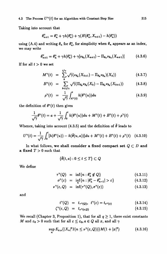
Taking into account that
using (AA) and writing On for 0;., for simplicity when On appears as an index, we may write
~+t = fr,. + ,h(fr,.) + ,[VSn(Xn+t) - I1sn VSn(Xn+t)]
If for all t > 0 we set
th = E..fY(V6.(Xk+t) - I1s.vs.)(Xk))
k
= E v'1(I1S.VII.(Xk) - I1s.VS.(Xk+l)) k<th
= ~ r h(O'"Y(u))du v' JA.,(t)
the definition of 8'"Y(t) then gives
Whence, taking into account (4.3.5) and the definition of 0 leads to
(4.3.6)
(4.3.7)
(4.3.8)
(4.3.9)
In what follows, we shall consider a fixed compact set QeD and a fixed T > 0 such that
We define
and
{O(t,a):O~t~T}cQ
r'"Y(Q) u'"Y(e)
v'"Y(e, Q)
= inf{n: fr,. ~ Q} = inf{n: Ifr,. - ~-11 > e}
n
= inf(r'"Y(Q),u'"Y(e))
t'"Y (Q) = t,,"(Q). t'"Y (e) = to""(~)
C(e, Q) = tll.,(~,Q)
(4.3.11)
(4.3.12)
( 4.3.13)
(4.3.14)
(4.3.15)
We recall (Chapter 3, Proposition 1), that for all q ~ 1, there exist constants M and eo > 0 such that for all e ~ eo, a E Q all x, and all,
sup Ex,a{IXnlqI(n ~ v'"Y(e,Q))}M(1 + Ixlq) (4.3.16) n
316 4. Gaussian Approximations to the Algorithms
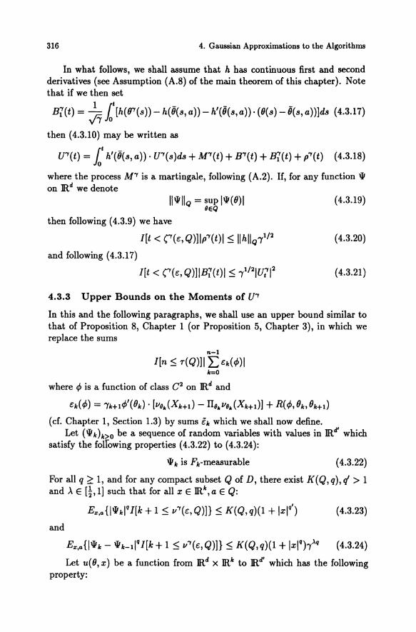
In what follows, we shall assume that h has continuous first and second derivatives (see Assumption (A.8) of the main theorem of this chapter). Note that if we then set
B'{(t) = .);y l' [h( ffY(s)) - h( O(s, a)) - h'(O(s, a))· (O(s) - O(s, a ))lds (4.3.17)
then (4.3.10) may be written as
U'Y(t) = l' h'(O(s,a)). U'Y(s)ds + M'Y(t) + B'Y(t) + B'{(t) + p'Y(t) (4.3.18)
where the process M'Y is a martingale, following (A.2). If, for any function W on R d we denote
IlwllQ = sup Iw(O)1 seQ
then following (4.3.9) we have
I[t < (Y(c,Q)llp'Y(t)1 :5l1hIlQ')'I/2
and following (4.3.17)
I[t < (Y(c, Q)lIB'{(t)1 :5 ,),1/2IU712
4.3.3 Upper Bounds on the Moments of U'Y
( 4.3.19)
(4.3.20)
(4.3.21)
In this and the following paragraphs, we shall use an upper bound similar to that of Proposition 8, Chapter 1 (or Proposition 5, Chapter 3), in which we replace the sums
n-l
I[n :5 r(Q)lI I>,,(¢)I 10=0
where ¢ is a function of class C2 on Rd and
c,,(¢) = ')'''+1¢'(O,,). [vsk(X"+1) - ITskvsk(Xk+dl + R(¢,O",O"+I)
(cf. Chapter 1, Section 1.3) by sums e" which we shall now define. Let (w"),,>o be a sequence of random variables with values in Rd' which
satisfy the folfowing properties (4.3.22) to (4.3.24):
w" is Flo-measurable (4.3.22)
For all q ~ 1, and for any compact subset Q of D, there exist K(Q, q), q > 1 and A E [~,11 such that for all x E R",a E Q:
(4.3.23)
and
E.",.{lw" - w"_llqI[k+ 1:5 v'Y(c,Q)]}:5 K(Q,q)(l + Ixlq)-y"q (4.3.24)
Let u(O, x) be a function from Rd x Rio to Rd' which has the following property:
4.3 The Process U'Y(t) for an Algorithm with Constant Step Size
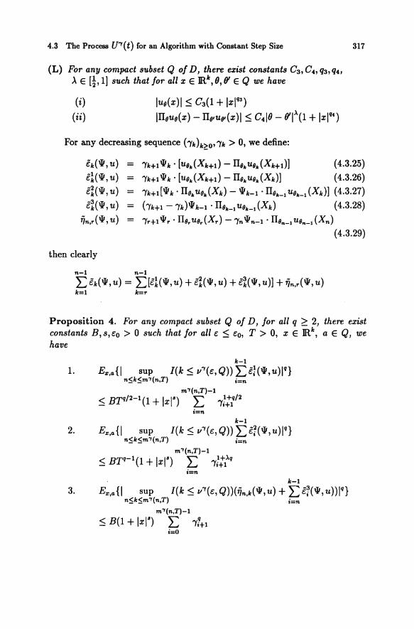
(L) For any compact subset Q of D, there exist constants C3 , C., Q3, q., A E [t,l] such that for all x E m\ 0, 0' E Q we have
(i)
( ii) lue(x)1 ~ C3 (1 + Ixlq3 )
IIIeue(x) - IIe1uel(x)1 ~ C.IO - 0'1,\(1 + Ixlq4 )
For any decreasing sequence (-y"h~o""y" > 0, we define:
317
€,,(w, u) = 'Y"+1w,,· rue. (X,,+d - IIe. ue. (Xk+1)] (4.3.25)
€l(w,u) = 'Yk+1W,,· [ue.(X"+1) - IIe.ue.(X,,)] (4.3.26) €%(w, u) = 'Yk+tlw,,· IIekuek(X,,) -W"_1 . IIek_1 uek_l (X,,)] (4.3.27) €%(w,u) = (-Y"+1-'Y,,)w"-1·IIek_luek_l(X,,) (4.3.28)
~n,r (w, u) = 'Yr+1W r . IIer uer (Xr) - 'Yn W n-1 . IIen_l uen_l (Xn) (4.3.29)
then clearly
n-1 n-1 E €,,(w, u) = E[€l(w, u) + €%(w, u) + €%(w, u)] + ~n,r(w, u) "=1 "=r
Proposition 4. For any compact subset Q of D, for all q ~ 2, there exist constants B,s,eo > ° such that for all e ~ eo, T > 0, x E R", a E Q, we have
"-1 1. Ex,a{1 sup I(k:$ 1I'Y(e,Q)) E€Hw,uW}
n:S;":S;m"Y(n,T) i=n m"Y(n,T)-1
~ BTq/2-1(1 + Ixn E 'Y::1q/2 i'=n
"-1 2. Ex,a{l sup I(k~II'Y(e,Q))E€Hw,uW}
n:S;":S;m"Y(n,T) i=n m"Y(n,T)-1
~ BTq-l(l + Ix I") E 'Ylt1'\Q i=n
"-1 3. Ex,a{1 sup I(k ~ 1I'Y(e,Q))(~n,,,(W,u) + E€~(w,u)W}
n:S;":S;m"Y(n,T) i=n m"Y(n,T)-1
~ B(l + Ixl") E 'Y?+1 i=O
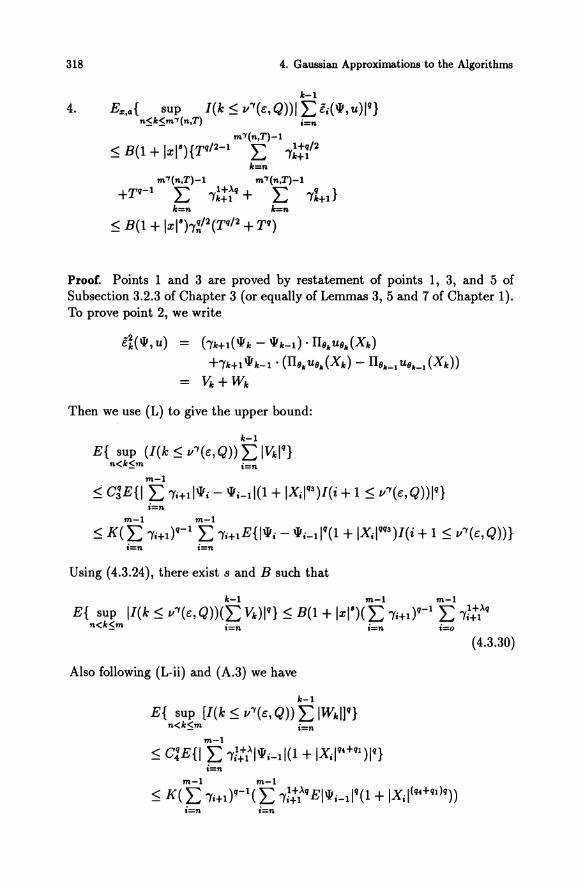
318 4. Gaussian Approximations to the Algorithms
k-1 4. E""a{ sup I(k~v"'(e,Q»/Eei('I,uW}
n~k~m"'(n,T) ;=n
m"'(n,T)-1
~ B(l + /xn{Tq/2-1 E 'Y!t~/2 k=n
m"'(n,T)-1 m"'(n,T)-1
+Tq-1 E 'Y!t~q + E 'Y%+1}
Proof. Points 1 and 3 are proved by restatement of points 1, 3, and 5 of Subsection 3.2.3 of Chapter 3 (or equally of Lemmas 3, 5 and 7 of Chapter 1). To prove point 2, we write
e%('I,u) = (-rk+1('Ik - IIIk-t)· TIOkUOk(Xk) +'Yk+1'1k-1· (TIOkUOk(Xk) - TIOk_1UOk_l(Xk»
= VI. + Wk
Then we use (L) to give the upper bound:
k-1 E{ sup (I(k ~ v"'(€, Q» E /Vkn
n<k~m i=n m-1
~ CjE{/ E 'Y;+1/ III; - '1;-1/(1 + /X;/q3)I(i + 1 ~ v"'(€,Q)W} i=n
m-1 m-1 ~ K( E 'Yi+dq- 1 E 'Yi+1 E {/III; - lIIi - 1/q(1 + /X;/Qq3)I(i + 1 ~ v"'(€, Q))}
i=n i=n
Using (4.3.24), there exist sand B such that
k-1 m-1 m-1 E{ sup /I(k ~ v"'(€, Q))(E VkW} ~ B(1 + /xn( E 'Y;+t}Q-1 E 'Y11tQ
n<k~m ;=n ;=n ;=0
(4.3.30)
Also following (L-ii) and (A.3) we have
k-1 E{ sup [I(k ~ v"'(e, Q» E /Wk/1Q}
n<k~m ;=n m-1
~ C!E{/ E 'Y111"/111;-1/(1 + /Xi /Q4+Q1W} i=n
m-l m-l
~ K(E 'Yi+t}Q-l(E 'YI:l"QE/III;-l/Q(1 + /Xi/(Q4+Ql)q» i=n i=n
4.3 The Process U'Y (t) for an Algorithm with Constant Step Size 319
Using property (4.3.23), there exist s and B such that
k-l
E{ sup II(k ~ V'Y(e, Q) E Wkl q } n~k~m ;=n
m-l m-l
~ B(l + Ixn( E -Yi+l)q-l E -y::l'q (4.3.31) i=n i=n
Point 2 of the proposition may now be deduced from (4.3.30) and (4.3.31). Point 4 is an immediate consequence of the decomposition of €k(\II,U) and of points 1 and 3 of the proposition. 0
Proposition 5. Let Q' be a compact subset containing Q, with
f3 = inf{lx - x'i : x E Q, x' ¢ Q'} > 0
Then for all q ~ 1, there exist s and a constant C depending only on Q, Q', q and e, such that for all 6 > O,t ~ O,a E Q',x E]Rk
a.
b.
Proof.
Ex,a{ sup I(M'Y + B'Y + p'Y)(u 1\ C(e,Q')) t~u9+6
-(M'Y + W + p'Y)(t 1\ C(e, Q')W} ~ C(l + Ixn(6Q/ 2 + -yq/2 + 6Q)
Ex,a { sup IU'Y( U 1\ C(e, Q')) - U'Y(t 1\ C(e, Q')W} t~u9+6
~ C(l + Ixn[(6 V -y)Q/2 + 6Q]
a. Applying Proposition 4-1 to the case u( 9, x) = v( 9, x), where v( 9, x) is the function of (A.4) and \II k = 1 gives the existence of C and s such that
Ex , .. { sup IM'Y(ul\u(e,Q'))-M'Y(tl\u(e,Q'))n t~u9+6
, ~ C(l + Ixn6q/ 2
Proposition 4-4 gives
(4.3.32)
Ex, .. { sup I(M'Y + W)(u 1\ C(e, Q')) - (M'Y + B'Y){t 1\ C{e, Q')W} t~u9+6
m"'(t+6) q
=-y-q/2Ex , .. { sup I[k+1~v'Y(e,Q')1I L €;(l,v)l} m"'(t)~k~m"'(t+6) ;=m"'(t)
~ B(l + Ixnw/2 + 6q ) (4.3.33)
320 4. Gaussian Approximations to the Algorithms
where v denotes the function v(O,x) = v/l(x). The first part of Proposition 5 follows from this inequality and from
sup 1P""'(t)I ~ ..n sup Ih(O)1 t:5("Y(~.Q') /leQ'
(4.3.34)
b. Using (4.3.10) and part a of the proposition, together with the fact that for u < '""Y(c, Q'):
Ih(tr'(u)) - h(6(u, a))1 ~ -y1/2 sup Ih'(O) II U""Y(u) I /leQ'
for some suitable constant K we have:
Point b of the proposition follows using Gronwall's Lemma.
Proposition 6. Let Q' be a compact set containing Q with
(3 = inf {Ix - x'i : x E Q, x' ¢ Q'} > 0
(4.3.35)
o
Then for all q ~ 2, t > 0 and c ~ co(q, Q'), there exist constants K > 0 and s ~ 0 such that for all a E Q and all x
Proof. Using Lemma 9 of Chapter 3, we have
(4.3.36)
then from Lemma 11 of the same chapter we have
Ex •a{ sup Itr'(t) - 6(t, aWl t<T 1\("y(~.Q')
~ A2(1 + IxI62 )(1 + T)q-l exp(qL2T)T-yq/2
Since 6(t, a) E Q for all t ~ T and a E Q we have
p",.a{f""Y(Q') < t""Y(c),t""Y(Q') < T}
~ ;: (1 + IxI62 )(1 + T)q-l exp(qL2T)T-yqI2 (4.3.37)
The inequality in the proposition follows from (4.3.36) and (4.3.37). 0
4.4 Gaussian Approximation of the Processes U'" ( t) 321
4.4 Gaussian Approximation of the Processes U"Y(t)
4.4.1 Assumptions
We shall add the following assumptions to those of Section 3.1.
(A.8) The function h has continuous first and second order derivatives, for all 0 ED, there exists a unique symmetric d X d matrix (Jlii (0», and for all (0, x), there exists a matrix (wij (0, x» such that (where liS is the function of (A.4)) (i) Jlij is locally Lipschitz on D (ii) (I - n,)w~(x) = n,/~,),(x) - nSIl~(x)ns,),(x) - Jlij(O) (iii) For any compact subset Q of D, there exist constants K 3 , K 4 , P3, P4,
Il E [1/2,1] such that, for all 0, fY E Q we have
Iw~(x)1 $ K3(1 + Ixl"3) In,w~(x) - n"w¥.(x)1 $ K4 10 - fJ'1"(1 + Ixl"4)
(4.4.1) (4.4.2)
4.4.2 Remark on Assumption (A.8) and Interpretation of R(O)
It is important to note that in the common situation in which the Markov chain with transition probability n, has a distribution with an invariant probability r" the matrix R(O) of Assumption (A.8), is exactly the same matrix R(O) as given in Part I, Chapter 3, Theorem 1.
Let us suppose now, as we did in Chapter 1, Section 1.3, comment c) that the Markov chain with transition probability ns has an invariant probability r, for which we write as usual
h(O) = J H(O,y)r,(dy)
and that the solution II, of the Poisson equation
(II, - n,II,) = H, - h(O)
is given by 1I,(y) = E n:(H, - h(O»(y)
k~O
Since r, is invariant for n" equation (A.8-ii) shows that
Ej(O) = J[II~,),(x) - n",~(x)n,,),(x)]r,(dx)
We may write
Rii(O) = J 1I~(x)(II~(x) - n,/~(x»r,(dx)
+ J 1I$(II~(x) - n,II~(x»r,(dx)
- J(II~(x) - n,/~(x»(,),(x) - n,II$(x»r,(dx)
(4.4.3)
(4.4.4)
(4.4.5)
322 4. Gaussian Approximations to the Algorithms
Then using (4.4.3) and (4.4.4) we have
Ei(O) = L J TI~(H~ - hi(O))(x)(Ht(x) - hi(O))r9(dx) "'~o
+ L J TI~(Ht - hi(O))(x)(H~(x) - hi(O))r9(dx) "'~o
- J(H~(x) - hi(O))(Ht(x) - hi(O))r9(dx)
Suppose that (X!)ne71 is a stationary Markov chain with transition probability TI9 and invariant probability r 9 • Then
. 9 . 8 cov[H'(O, X",), HJ(O, Xo)] ·9· 9 = cov[H'(O, Xo), HJ(O, X_",)]
Whence 00 Rii(O) = L cov[Hi(O,XZ),Hi(O,Xg)] (4.4.6)
"'=-00 This is exactly the corresponding formula of Theorem 1 of Part I, Chapter 3.
4.4.3 Gaussian Approximation Theorem
Theorem 7. Under Assumptions (A.2), (A.B), (A.4), (A' .5) and (A.B), the distributions (Pi a) 0 of the processes U"I converge weakly as "'I -+ 00 to the , "I> distribution of the Gaussian diffusion with initial condition 0 and generator L t given by:
LtW(x) = taiW(X)[taihi(O(t,a))xi] + ~.t aliw(x)Rii(O(t,a)) ,=1 J=1 ',J=1
Proof of Theorem 7. The proof is divided into two stages. Stage 1. The family of distributions (Pi a) 0 is tight. , "I> Stage 2. If P is any limiting distribution for the family (jJ'Y), then P satisfies the martingale condition:
is a martingale for any function W of class C2 with compact support. Following Section 4.2 (above), this characterises any limiting distribution
of the sequence (Pi,a)"I>O as the unique distribution of the Gaussian diffusion with initial condition 0 and generator Lt.
4.4 Gaussian Approximation of the Processes lj'''I(t) 323
Weak compactness 0/ the distributions P;,a. In order to prove the compactness, it is sufficient to prove that the following hold for some q ~ 1 and p > 1:
lim Pxa{(Y(c:, Q) < T} = 0 "'I~O '
and for all 6 > 0 there exists n6 such that
sup sup Ex,a{ sup 1U'Y(s" (Y) - U'Y(t" (YW} ~ 6P
tE[O,T] n~n6 t:S;$:S;t+6
In fact, from conditions (4.4.7) and (4.4.8), it is easy to see that
lim supPxa{IUiI > r} = 0 T--+OO 'Y t
This is condition [T l ] of Subsection 4.1.3 Condition (4.4.9) implies that for all n ~ n6 and t ~ T
1 6P- l 1 cPx,a{ sup IU'Y(s) - U'Y(t)1 ~ 77} ~ - + cPx,a{(Y < T} v t:S;$:S;t+6 77 v
(4.4.7)
(4.4.8)
( 4.4.9)
This inequality and (4.4.7) together imply condition (4.1.5) for the sequence Pi,a' This proves that the distributions P::,a are compact.
Identification 0/ the Limit.
Following the remark in 4.1.4, we know that any limit P of a convergent sequence j)'Yn is carried by C([O, T]j JRd). We shall show further that such a limit P is such that, for any \Ii of class C2 with compact support, the process
is a martingale on (fh, (Ft)t<T' P). For this, it is sufficient to show that for all s ~ t ~ T, for all functio;s / on fh of the form
where the hi are continuously bounded, we have
(4.4.10)
Since by construction, the restriction of / to C([O, T]j JRd) is continuous, we see that
324 4. Gaussian Approximations to the Algorithms
defines a continuous function in C([O, T]; JRd). Since P[C([O, T]; JRd)] = 1, following the remark of Subsection 4.1.4, we have:
= lim kYn( c)) n
= li,?lEz.a{([J(U'Y)][\II(U;') - \II(U'1) -[ Lu\ll(UJ)du]}
Since, by construction J(U'Y) is F3-measurable and bounded, we will have proved (4.4.10) if we can show that
\II(U;') = \II(Uri) + l Lu\II (UJ)du + N? + Jq (4.4.11)
where N'Y is a martingale and
lim EIJq /\ (y1 = 0 '1'-+0
( 4.4.12)
since then we have
Ez.a{([J(U'Y)][\II(Ui) - \II(U'1) -[ Lu\ll(UJ)du]}
~ IIJlloo[E(IRi"(l1 + IR;",..,I) + (211\111100 + It - sIIlLu\lllloo)Px.a{(Y < T}]
Thus in order to prove the theorem, it is sufficient to prove (4.4.11) and (4.4.12) ..
Note that
\II(U'l(t)) = \II(U'Y(O)) + E (\II(U'Y(tk)) - \II(U'Y(tk-d) + r(t) ( 4.4.13) k9h
where II Ir(t)1 = -I h(O(s))dsl ~ .j7sup Ih(x)1 .j7 A..,(t) xEQ
(4.4.14)
We write U'Y(tk) - U'Y(tk_d = ~7(k) + ~;(k) (4.4.15)
where S{(k) = [k h(frY(s)) - h(O(s, a)) ds
tk_l ..fY (4.4.16)
and ~;(k) = .j7[H(Ok-t,Xk) - h(Ok-d] (4.4.17)
Notation.
1. For simplicity, in what follows, we shall denote any process Zt such that
EIZt"(l1 < K'y" for all t ~ T
for some constant K, by Otb"').
4.4 Gaussian Approximation of the Processes U'Y(t)
2. For any matrix (xii and any vector v we denote
a 0 V®2 = Eaiivivi
We then see that
'II(U'Y(t)) = 'II(U'Y(O)) + E 'II'(U'Y(tlc_I))· (~I(k) + ~;(k)) 1c9h
+~ E 'II"(U'Y(t lc_d) 0 (~1(k))®2 lc<S.th
325
+Ot(v0") (4.4.18)
Lemma B.
E 'II'(U'Y(tlc+d)· ~1(k)= l 'II'(U'Y(s)). [h'(6(s,a)) 0 U'Y(s)]ds+Ot(v0") 1c9h 0
Proof of Lemma 8. This lemma follows from the definition of
I tk ~1(k) = tk-l h'(6(s,a)) 0 U'Y(s)ds + pi
with
IpiA("II::; -21 v0" sup 1h"(O)1 sup IU'Y(s) 12 8EQ' tk_l <s"9k
Lemma 8 now follows from Proposition 5-b with t = 0 and 8 = T. 0
Lemma 9.
E 'II'[U'Y(tlc_I)]· ~l(h) 1c9h
d
= Ml(t) + E E a?;'II(U~_l) . ~;,i(k) . II8k_1 vt_l (XIc) + Ot( v0") 1c9h i ,j=1
where Ml is a martingale
Proof of Lemma 9. We write
and decompo,se
E 'II'(U'Y(tlc_I))· ~1(k) 1c9h
= E v0"'II'(U'Y(tlc_d)· [V8k_l (XIc ) - II8k_1 V8k_1 (XIc-d] 1c9h
(4.4.19)
+ E v0"[IlI'(U'Y(tlc_d)· II8k_l V8k_1 (XIc_d- IlI'(U'Y(tlc)) . II8k-lV8k_l(XIc)] 1c"9h
+ E v0"[IlI'(U'Y(tlc)) - 'II'(U'Y(tlc_d)]· II8k_1 V8k_l (XIc ) 1c9h
326 4. Gaussian Approximations to the Algorithms
The first term on the right hand side of this equation defines the martingale Mi-
The upper bounds of points 2 and 3 of Proposition 4 may be applied to the second term to show that this term is Oky>')
Finally, the third term may be written as
d
L ..fi L at;\If(u'Y(tk-d)A1"(k)IIok_1 vZk_1 (Xk) + Ot(..fi) k9h ',;=1
o
Lemma 10.
~ L t a?; \If[U'Y(tk_d]· [A1"(k)A1';(k) + 2..fiA1"(k)IIok_1 {-I (Xk)] k'5.th·,;=1
= l Trace \If"[U'Y(s)] 0 R[O(s)]ds + Ml(t) + Ot(..fi)
where Ml is a martingale.
Proof of Lemma 10. If we write A1(k) in the form (4.4.19), then using Assumption (A.8), the expression in the lemma may be written as
~ L 'Y t al,;\If(U'Y(tk_1)) k'5.th ',;=1 [V~k_l (Xk)V~k_1 (Xk) - IIok_1 V~k_l (Xk)IIok_1 vtl (Xk)]
= ~ L 'Y Trace \If"(U'Y(tk_1)) 0 R(O(tk-d) k9h
+ L 'Y\If"(U~_I)· [WOk_1 (Xk) - IIok _ 1 WSk_1 (Xk)]®2 k9h
Lemma 10 then follows using Proposition 4-4.
Lemma 11.
l Trace \If" (U'Y (s)) 0 R( O( s ))ds
= l' Trace \If"(U'Y(s)) 0 R(O(s, a))ds + Ot(..fi)
Proof of Lemma 11. Since h is Lipschitz
1 r Trace \If"(U'Y (s)) 0 (R( O( s)) - R( O(s, a)) )dsl ::; K..fiT sup 1U'Y(s)1 10 '9
Lemma 11 follows from Proposition 5.
o
o
4.4 Gaussian Approximation of the Processes U'Y(t) 327
Proof of Theorem 7 (Continued). If we now rewrite (4.4.18,) using Lemmas 8 to 11, we see that
This is formula (4.4.11) and thus Theorem 7 is proved. o
4.5 Gaussian Approximation for Algorithms with Decreasing Step Size
4.5.1 The Problem-Assumptions
We now consider an algorithm with decreasing step size ('Yn):
(4.5.1)
In Chapter 1, Subsection 1.5.3, we introduced the algorithms (ON+n)n>O where PN,x,a denotes the distribution of the sequence (ON+n)n~o satisfying -
{ ON+n+1 = ON+n + 'YN+n+1 H(ON+n, X N+n+1) ON = a X N = X
(4.5.2)
We studied the behaviour of the algorithms (4.5.2) as a function of N. More generally, we might also consider a sequence (O~)n>o N =0, ... , k, ...
of algorithms of the form -
(4.5.3)
where the X N are associated with the same transition probability IIe(x, dy), o E IRd. Then, if as in Subsection 1.1.1, we set
n
tN = L 'Y[" ( 4.5.4) n k~O
ON(t) L I(tf ~ t < tf+1)Of (4.5.5) k~O
mN(n, t) = inf{k: k ~ n,'Y~+l + ... + 'Yf-t.l ~ T} (4.5.6) mN(T) = mN(O,T) (4.5.7)
then under the assumptions of Theorem 9 of Chapter 1, we have
328 4. Gaussian Approximations to the Algorithms
for all D > 0, where iJ(t~j a) denotes the solution of the ODE
{ :8~r) = h(iJ(tj a)) 6(Oja) = a
(4.5.8)
associated with H and (II8)8ER". Thus, analogously to Section 4.4, it is possible to study the weak convergence as N -+ 00 of the sequence of processes UN defined by
where
UN (t) = oN (t) - iJ(t, a) V-yN(t)
-yN (t) = E I(t~ ~ t < t~+lh~ k~O
This problem is discussed in Subsection 4.5.2
(4.5.9)
(4.5.10)
Following on from this, in Subsection 4.5.3, we shall obtain a Gaussian approximation result for the vectors -y;1/2(6(n) - 6.) in the case of an algorithm (4.5.1) converging to 6.. As far as the sequences b:)n>o are concerned, we shall assume that they are decreasing, that limN_oo -y~ = 0 and that there exists a ~ 0 such that
1· IR-~ -I 0 1m sup / - a = N_oo k b~1)3 2
(4.5.11)
Remark. If -y;: = (N:n)P, it is easy to see that if f3 = 1 then a = 1/2 and that if f3 < 1 then a = o.
4.5.2 Sequence of Algorithms with Decreasing Step Size. Gaussian Approximation Theorem
We shall prove the following result.
Theorem 12. We assume that the function H, the sequences b:)n>ON E 1N and the transition probabilities (II8)8ER" satisfy (A.i) to (A.4). (A'.5) and (A.B).
1. The, distributions (P:'a)N>O of the processes UN converge weakly as N -+ 00 to the distribution of the Gaussian diffusion with initial condition 0 and generator Lt given by
4.5 Gaussian Approximation for Algorithms with Decreasing Step Size
2. We suppose that the random variables 0:, N ~ 0 are such that the
distribution of the sequence (Uf)N>O = [b:)-1/2.(0: - OO)]N>O converges weakly towards a distribuTion v. We also suppose that for any compact set Q I we have
sup E{IUfI2 /(0: E Q)} < 00 N
Then the sequence of distributions of the processes UN, N ~ 0 converges weakly as N -+ 00 to the distribution of the diffusion with initial condition v and generator Lt.
329
Proof. Point 1 is clearly a special case of point 2. The proof of point 2 follows the same strategy as the proof of Theorem 7. We modify equations (4.3.5) to (4.3.10) as follows
o~ + "'{t;+1 h(ot;) + "'{t;+1[V8ir(X~1) - II8irV8ir(X~1)]
1: J"'{~+1[V8k(X~1) - II8kv8k(Xf)] (4.5.12) k;5mN(t)
1: J"'{~+1[II8kv8k(Xf) - II8kV8k(X~1)] (4.5.13) k;5mN(t)
l (k>h(ON(U)) + aN(U)UN(U)) du (4.5.14) AN(t) "'{N(u)
where AN(t) = max{tf:jtf: ~ t}. If we set
(4.5.15)
then we have
whence
330 4. Gaussian Approximations to the Algorithms
If we set
N() ~ (N N )R-~ o t = LJ I tic ~ t < tlc+l (N )3/2 Ie 'Ie+l
(4.5.16)
then formula (4.3.10) for algorithms with constant step size is replaced here by
UN(t) = UN(O) + lON(S)UN(S)ds
+ It ~[h((r(S)) - h(O(s,a))]ds 10 ,N(s)
+MN(t) + BN(t) + pN(t)
This gives the formula analogous to (4.3.18);
UN(t) = UN(O) + loN(s)UN(s)ds+ lh'[O(s,a)]oUN(s)ds
+MN(t) + BN(t) + Bf(t) + pN(t) (4.5.17)
where
Bf(t)= r ~[h((}N (s))-h(O(s, a))-h'(O(s, a)).((}N(s)-O(s, a))]ds 10 ,N(s)
Next we give definitions analogous to (4.3.11) to (4.3.15)
rN(Q) = inf{n;(}~ ll' Q} ~(c:) = inf{n;I(}~-(}~_ll>c:}
IIN(c:,Q) = inf(rN(Q),~(c:))
(N (c:, Q) = t'YN(~.Q)
The definitions of pN and Bf show that
I{t < (N(c:,Q)} ·lpN(t)1
(4.5.18)
(4.5.19)
(4.5.20)
(4.5.21)
(4.5.22)
~ IIhIIQb(t))1/2 + ,(t) sup II[s < (N(e, Q)]on(s)U'Y(s)1 (4.5.23) 69
and
We note here that the upper bounds in Proposition 4 were derived (d. definitions (4.3.25) to (4.3.29)) for algorithms with decreasing gain. Thus the same inequalities as in Propositions 5 and 6 may be directly inferred
4.5 Gaussian Approximation for Algorithms with Decreasing Step Size 331
by replacing M"f,U"f,B"f and p"f by MN,UN,BN and pN (respectively) . In particular, if Q' is a compact set containing Q for which
fJ = inf{lx - x'i : x E Q, x' ¢ Q'} > 0
there exist constants C > 0, s > 0 such that for all N, t > 0, 6> 0 and q ~ 1:
E{ sup IUN(uA(N(e,Q'))-UN(tA(N(e,Q'))lq} t5u9+6
~ C(l + Ixn(6 V "'If)q/2 (4.5.25)
As in the proof of Theorem 7, we now deduce that there exist q ~ 1 and p > 1 such that for all 8 > 0 there exists n6 such that for all N
sup sup E{ sup IUN(s A (N) - UN(t A (NW} ~ 6P (4.5.26) tE[O,T) n~n6 t589+6
As in Proposition 6, we have
lim p{(N(e,Q) < T} = 0 N ..... oo
(4.5.27)
The assumption
supE{IUt'12/(O: E Q)} < 00 N
together with (4.5.25) shows that
supE{ sup IUN(t A (N(e,Q'))12 } < 00 N 095T
As in the proof of Theorem 7, the weak compactness of the sequence pN of the distributions of processes UN follows immediately.
The limit is determined as in the proof of Theorem 7 by writing:
w(UN(t)) = w(UN(O)) + ~ w'[UN(tf_l)]' [~f(k) + ~f(k)] k5m N (t)
+~ ~ w"[UN(tf_l)] 0 [~f(k)]®2 + Ot(v,f) k5m N (t)
where
~f(k) = 1tk aN(s)UN(s)ds + 1tk h«(}N(s)) - h(iJ(s,a))ds tk_1 tk_I"; "'IN ( s )
and ~f(k) == R[H«(}k-l,Xk) - h«(}k-t}]. We see that Lemmas 8 to 11 may be applied word for word to show that
w(U{") = w(Ut') + l Luw(U:)du + N{" + Rf where NN is a martingale and
lim EIR~"N I = 0 N ..... oo '
The proof is now completed as for Theorem 7. o
332 4. Gaussian Approximations to the Algorithms
4.5.3 Gaussian Asymptotic Approximation of a Convergent Algorithm
In this paragraph, we shall consider an algorithm (On) which converges almost surely, under the assumptions at the end of Chapter 1. More precisely, we shall suppose that the algorithm (4.5.1) satisfies Assumptions (A.l) to (A.5) of Chapter 1, and that if TR denotes the time at which On leaves the compact set {101 :::; R}, then
inf PI: .. {TR < oo} = 0 R>O '
(4.5.28)
In particular, this condition is satisfied by any system whose assumptions include the a.s. boundedness of (On) (c.f. Section 1.9 of Chapter 1) We shall also suppose that the following two conditions are satisfied
r V7n - y-y;::;t n~~ 3/2
In+!
(4.5.29)
(0 - O.).h(O) (4.5.30)
with lim inf 28 ~ + In+!2 - In > 0
n .... oo In+l In+l (4.5.31)
Then we have the theorem:
Theorem 13 We assume the conditions listed above hold, and that, in addition, the eigenvalues of the dxd matrix B with terms Bij = ii8ij+8jhi(0.), i, j = 1, ... , d all have strictly negative real parts. Then we have
1. The sequence pN of the distributions of the processes defined by
converges weakly towards the distribution of a stationary Gaussian diffusion with generator
1 ~ ., L\II(x) = Bx· V\II(x) + - L..J 8?;\II(x)R"(0.)
2 .. 1 1,1=
2. The sequence of random variables
n E 1N
(4.5.32)
converges in distribution to a zero-mean Gaussian variable with covarzance [00 T
C = Jo e3B 0 R 0 e3B ds (4.5.33)
4.5 Gaussian Approximation for Algorithms with Decreasing Step Size 331
by replacing M"",U\B"" and p"" by MN,UN,BN and pN (respectively) . In particular, if Q' is a compact set containing Q for which
f3 = inf{lx - x'i : x E Q,x' f/. Q'} > 0
there exist constants C > 0, s > 0 such that for all N, t > 0, 6 > 0 and q ~ 1:
E{ sup IUN(u,,(N(e,Q'))-UN(t,,(N(e,Q'))lq} t~,,~t+6
~ C(1 + Ixn(6 V ,i")Q/2 (4.5.25)
As in the proof of Theorem 7, we now deduce that there exist q ~ 1 and p > 1 such that for all 6 > 0 there exists n6 such that for all N
sup sup E{ sup IUN(s" (N) - UN(t" (N)lq} ~ 6P (4.5.26) tE[O,T) n~n6 t~B9+6
As in Proposition 6, we have
lim p{(N(e,Q) < T} = 0 N-oo
(4.5.27)
The assumption
supE{IUt'12/(O~ E Q)} < 00 N
together with .(4.5.25) shows that
sup E{ sup IUN (t " (N (e, Q'))12 } < 00 N 09~T
As in the proof of Theorem 7, the weak compactness of the sequence pN of the distributions of processes UN follows immediately.
The limit is determined as in the proof of Theorem 7 by writing:
W(UN(t)) = W(UN(O)) + E W'[UN(tt'_l)]· [~f(k) + ~f(k)] k~mN(t)
+~ E W"[UN(tt'_l)] 0 [~f(k)1®2 + Ot(R) k~mN(t)
where
~f(k) = ltk o:N(s)UN(s)ds + ltk h(ON(s)) - h(iJ(s,a))ds tk_l tk-1"'; ,N (s)
and ~f(k) = ..:j:;N[H(Ok-l,Xk) - h(Ok-d]. We see that Lemmas 8 to 11 may be applied word for word to show that
w(Ut') = W(Ut') + l L"W(U:)du + Nt' + R,/
where NN is a martingale and
lim EIR~ml = 0 N_oo ~
The proof is now completed as for Theorem 7. o
334 4. Gaussian Approximations to the Algorithms
It follows, letting tk tend to +00, that
for all e > O. Condition (4.5.35) now follows, as do the lemma and Theorem 13. o
Remark. It can be shown by elementary integration that
BC + CBT = Lco[B 0 e3B 0 R 0 e3BT + e3B 0 R 0 e3BT 0 BT]ds = -R
The matrix C defined in (4.5.33) is thus a positive symmetric solution of the Lyapunov equation
as indicated in the statement of Theorem 3 of Chapter 3, Part 1.
4.6 Gaussian Approximation and Asymptotic Behaviour of Algorithms with Constant Steps
Theorem 13 says that for a class of algorithms with decreasing step size, the random variable ,;;1/2(On - 0.) converges in distribution to a Gaussian variable. In the case of algorithms (~) with constant step size " such as those considered in Subsection 4.4.3, it is reasonable to wonder whether, when the ODE has an asymptotically stable equilibrium point 0. (with additional assumptions in some cases), the random variable ,-1/2(~ - 0.) behaves asymptotically, for n large and , small, like a Gaussian variable. We shall formalise the property of this type cited in Theorem 2 of Chapter 3, Part I in the statement of Theorem 15 (below).
4.6.1 Assumptions and Statement of the Asymptotic Theorem
We assume the conditions of Sections 4.3 and 4.4 hold, with the following reinforcements:
(A-i). For all a E JRd
lim O(t,a) = 0. t_co
(A-ii). The matrix (ojhi(O) : i,j = 1, ... , d) lS Lipschitz in ° and the eigenvalues of the matrix B defined by
all have strictly negative real parts.
4.6 Gaussian Approximation for Algorithms with Constant Step Size 335
(B). There exist q}, q2, q3 ~ 0 and for all q > 0 and all compact sets Q, a constant ",(q, Q) such that for all "I ~ 1, x E ]Rd, a E Q:
( i)
( ii)
(iii)
(iv)
sup E."IJ(1 + IXJlq) ~ ",(I + Ixl q) n
sup E."IJ 11I8;t (XJ+1) 12 ~ ",(I + Ixlq2 ) n
sup E."IJI~12 ~ ",(I + Ixl q3 ) n
Theorem 15. We consider the stochastic algorithms (~) defined in (4.3.1) with the assumptions of Sections 4.3 and 4.4 reinforced by (A) and (B) (above). Then, for any sequence Tn i 00 and any sequence "In ~ 00, the sequence of random variables (U'Yn(Tn))n>O converges in distribution to a zero-mean Gaussian variable with covariance C where C is the matrix
C = 1000 exp·B Re·BT ds
where R is the matrix defined in Assumption (A.B).
Proof. This will be carried out in several stages. After examining several simple consequences of Assumptions (A) and (B), in (4.6.3) we shall derive an upper bound for EIUil2 involving the weak compactness of the distributions of the (U'Yn(Tn))n>O; we shall complete the proof in 4.6.4 using an argument similar to that oCLemma 14.
4.6.2 Initial Consequences of Assumptions (A) and (B)
Let {r(t,s) : s ~ t} be the resolvent, for fixed a, of the linear system
d~~t) = h'(6(t,a))x(t)
(d. (Reinhard 1982)). We recall that r(t,s) is a solution of the differential equation
dr(t,s) = h'(6(t,a))r(t,s), t ~ s dt
r(s,s) = Id
We also recall that the solution of the equation with second term
is given by
dx(t) = h'(ii(t, a))x(t)dt + dF(t), t ~ s
,x(s) = x.
x(t) = r(t,s)x.+ [r(t,u)dF(u) (4.6.1)
336 4. Gaussian Approximations to the Algorithms
and that this formula is valid not only when F is a function of finite variation for which the integral of the second term of (4.6.1) exists, but also for a stochastic differential equation in which F(t) is the sum of a martingale and a process whose trajectories are of finite variation. Thus it follows from (A-i) and (A-ii) that there exist numbers a > 0 and to such that for all t > to, the eigenvalues of h' (iJ( t, a» all have negative real parts ~ -a and that
IIr(t,s)1I ~ e-a(t-a) (4.6.2)
We now return to equation (4.3.18), writing, in conformity with equation (4.6.1 ):
(4.6.3)
where (4.6.4)
with the notation of Subsection 4.3.2. The process M'Y is a martingale (it is also a process with interval-wise constant trajectories, thus it is of finite variation). We also have
Bi(t) = l bi(s)ds
with, following (4.3.17), for some suitable constant K,
(4.6.5)
From the definitions of M'Y, ll'Y and p'Y, we deduce using Assumption (B) and denoting the jump in t of the process Z by 6.tZ :
sup(EI6.tM'Y12 + EI6.tll'Y12 + EI6.tp'Y1 2 ) ~ K'Y(1 + IxIP) t~O
(4.6.6)
for some suitable constant K, some (3 (in the remainder of this paragraph, we shall use K to denote any constant independent of 'Y).
Given a right-continuous function f on 1R+, we denote
w(j,b,s)= sup If(S/)-f(s)1 a~.'~.+6
From the definition of p'Y, we have
whence
EI f f(L)dp'Y(s)1 1],.,t]
1 it ~ ~ Elw(j,b,s)h(IP.)lds + -n sup Elf(s)h(IP.)1 v'Y ,. Ai~s<t
(4.6.7)
4.6 Gaussian Approximation for Algorithms with Constant Step Size 337
We shall use [M'Y] and [N'Y] to denote the so-called processes of "squarevariation" defined by
[M'Y]t = L: 1~.M'Y12 (4.6.8) ·9
and [N'Y]t = L: 1~.N'Y12 (4.6.9)
·9 Lastly, we recall that if V is an adapted process whose trajectories have a left limit Va- at all points and are integrable with respect to dMi and dNi then we have
(martingale property) and
EI f Va_dN:1 1]o,t]
E (f Va- dM:) = 0 1]o,t]
(4.6.10)
$ ft (EIV(sW)1/\ElbI(s)12)1/2 ds + E [EIV(L)12]1/2[EI~.N'Y12]1/2 10' .9
(4.6.11)
4.6.3 Upper Bounds for the Process U'Y
The strengthening of the assumptions on the moments afforded by condition (B) leads directly to the following reinforcement of Proposition 4:
Proposition 16 Let lk(v),li(v),i = 1,2,3,~n,k(v) be as defined in 4.3.3, taking q, = 1 and u to be the solution v of the Poisson equation in Assumption (A.4). Under the assumptions of 4.6.1 there exist constants B,/3 (depending on a) such that for all T > 0
k-l 2
(i) E""a(1 sup L:l:(v)l) $ BT(l + Ixl~h n~k~m"'(n,T) i=n
k-l 2
(ii) E""a(1 sup L: l~(v)1 ) $ BT2(1 + IxlPh 2 n~k~m"'(n,T) i=n
, k-l 2
(iii) E""a(l sup L: l~(v)1 + l~n,k(VW) $ B(l + Ixl~h2 n~k~m"'(n,T) i=n
k-l 2
(iv) E"" .. (I sup L: li(V)1 ) $ B(l + Ixl~)(T +, + ,T2) n~k~m"'(n,T) i=n
Proof. It is sufficient to follow the proof of Proposition 4 step by step, or even better Proposition 8 of Chapter 1 and the lemmas which precede it, together
338 4. Gaussian Approximations to the Algorithms
with all the intervening simplifications resulting from the assumptions in this case. Thus we have the following analogue of Proposition 5-a:
E""CJ sup IM'Y(u) - M'Y(t)12 < BT(l + Ixl13) (4.6.12) t~u9+T
E""CJ sup IA'Y(u) - A'Y(tW < B(l + Ixl13h(l + T2) (4.6.13) t~u9+T
and as in Proposition 5-b
(4.6.14)
o We shall now improve this estimate of EIU'Y(tW, making it independent
of T, using Assumption (A).
Proposition 17. Under the assumptions of this section, there exists 'Yo such that
Proof. A simple argument based on integration by parts (or on a classical formula for linear differential equations with a second term) gives from (4.6.3):
U'Y(t) = f(t,to)U'Y(to) + r f(t,s)dM'Y(s) + 1 f(t,s)dN'Y(s) (4.6.15) l)to,t) )to,t)
(Here we have U'Y(O) = 0). For u ~ t, we set
W'Y(u,t) = U'Y(to) + r f(u,s)dM'Y(s) + r f(u,s)dN'Y(s) l)to,t) l)to,t)
Applying Ito's formula (Metivier 1983) we have:
EIW'Y(u, t)12 = EIU'Y(to) 12 + 2E{ r (W'Y(u,s), f(u,s)dN'Y(s))} l)to,t)
+2E{ r Trace [f(u,s). fT(u,s)](d[M'Y]. + d[N'Y].n l)to,t)
Next we choose to so that (4.6.2) is true (in fact u = t) and apply (4.6.4) and (4.6.11). Then we obtain
EjU'Y(t) 12 ~ EIU'Y(to) 12
+2E{1 f [U'Y(s)]T 0 f(t,s) 0 bI(s)dsl} l)to,t)
+2E{1 r [u'Y(s)f 0 f(t,s) 0 dp;1} l)to,t)
+2E{1 r [u'Y(s_)]Tof(t,s)odB]ll l)to,t)
+2E{1 r e-a(t-')(d[M'Y]. + d[N'Y].n (4.6.16) l)to,t)
4.6 Gaussian Approximation for Algorithms with Constant Step Size 339
Following (4.6.5)
E{I I [U'Y(s)t.r(t,s).bI(s)dsl} ~ K I e-a(t-s)EIU712ds ~~~ ~~~
(4.6.17)
We now note that, following (4.6.14), for s ~ to
E sup I[U'Y(s')t· r(t,s') - [U'Y(s)]T. r(t,s)1 2
s~s'<s+6<t
~ K(l + Ixl.B)(-r V c5')e-2a(t-s) (4.6.18)
Following (4.6.14) and using the Lipschitz property of h, we have
sup EI[U'Y(s)t· r(t,s)· h(tr.)1 ~ K(l + Ixl.B)(l + vlrEIUiI2) (4.6.19) Al~s<t
Thus, following (4.6.7), (4.6.18) and (4.6.19) we have
E{I I [U'Y(s)t· r(t,s)· dp~1l ~ K(l+lxl.B) I e-a(t-·)(Elh(tr.)12)1/2ds ~~~ ~~~
+K(l + Ixl.B)(l + vlrEIUiI2)
or
E{I I [U'Y(s)t· f(t,s)· dp~1l l)to,t)
~ K(l + Ixl.B){ I e-a(t-s)(l + EItr.12)1/2 ds(l + vlrEIUiI2)} l)to,t)
(4.6.20)
Following (4.6.6) we have
2E{1 I [U'Y(L)t· r(t, s)dBill ~ l)to,t)
<
< K(l + Ixl.B)vIr It e-a(t-s)ds (4.6.21) lto
Lastly, also from (4.6.6), we obtain
E{I I e-a(t-·)(d[M'Y] + d[N'Y])} ~ K(l + Ixl.B) rt e-a(t-s)ds l)to ,t) B s lto
(4.6.22)
Regrouping the inequalities (4.6.16), (4.6.17) and (4.6.20) to (4.6.22) we have
EIU'Y(t)12 ~ EIU'Y(toW K(l + Ixl.B)(l + It et-sds) lto
+1((1 + Ixl.B)vlrEIU'Y(tW
340 4. Gaussian Approximations to the Algorithms
Thus if we choose 'Yo such that
1 - K(l + IxlP)y'1o := v > 0
then for all 'Y ~ 'Yo and all t, we have:
v . ElifY(tW ~ sup ElifY(toW + K(l + IxIP) 'Y
and Proposition 17 is proved.
4.6.4 End of the Proof of Theorem 15
We now consider sequences tn i 00, 'Yn L 00 and the processes
Following (4.6.3) we have
o
(4.6.23)
vn(t) = U'Yn(tn) + l h'(O·)Vn(s)ds + M'Yn(tn + t) - M'Yn(tn)
+N'Yn(tn + t) - N"ln(tn) + l(h'[O(tn + s,a)]- h'[O.Dds
The upper bounds on M"ln(tn + t) - M'Yn(tn) and N"ln(tn + t) - N'Yn(tn) derived in Section 4.3 enable us to carryover the arguments of Sections 4.4 and 4.5 almost word for word. Thus, if the sequence of random variables U'Yn(tn) (which is weakly compact by Proposition 17) converges in distribution to a distribution v, then the sequence of processes (vn) converges in distribution to a stationary Gaussian diffusion with generator
1 ~ 2 .. L¢>(x) = Bx· V¢>(x) + 2 .~ 8;j¢>(x)R'J(O.)
',J=1
(4.6.24)
and initial condition v where the matrix B is as defined in 4.6.1, Assumption (A-ii) and R(O.) is as defined in (A.8).
As in the proof of Lemma 14, for all e > 0 and all <Ii E CK(IRd), we can determine T so that for any v in the weak closure of the distributions of the variables {U"I(t)i'Y ~ 'Yo, t > O} the distribution PII(t) at time t of the diffusion (4.6.24) with initial condition v satisfies for all t > T
(4.6.25)
where 9 is the Gaussian distribution N(O, C), C being the matrix defined in Theorem 15. We now consider an arbitrary convergent subsequence (!J'Ynk (tnk)) with limiting distribution v. We merely have to show that for all e > 0
1(<Ii, voo ) - (<Ii,g)1 ~ e
Without loss of generality, without extracting a subsequence,we may suppose that (U'Ynk (tnk - T))k>O is itself weakly convergent towards a distribution v. This implies that Voo ;; PII(t). The result now follows from (4.6.25). 0
4.7 Remark on Weak Convergence Techniques 341
4.7 Remark on Weak Convergence Techniques
Kushner and Shwartz (1984) used a method of weak convergence to establish the approximation by the ODE. If we consider an algorithm with constant gain, as in (4.3.1), together with the corresponding process (}'Y(t) in continuous time, we see that the latter may be written as :
lJY(t) = lJY(O) + l' h(lJY(u»du + J1[lP(t) + p"'(t)] + martingale (4.7.1)
where the processes 1P, and p'" are those defined in formulae (4.3.8) and (4.3.9).
Kushner and Shwartz (1984) showed that the distributions of the processes ((}'Y) are weakly compact as "'( ! 0 and that any limiting distribution is a solution of the martingale condition
</>(O(t)) = </>(0(0» + l' h(O(u» . </>'(O(u»du + martingale (4.7.2)
Such a limiting process is associated with the differential operator
L</>(x) = h(x)· </>'(x)
which contains no diffusion terms. This is thus a process with deterministic trajectories which are solutions of the equation
O(t) = 0(0) + l' h(O(u»du
This brings us back to the ODE. If 0(0) = a, and if the ODE has a unique solution, then the convergence in distribution of the random function 0'" to a uniquely determined function 0 implies convergence in probability. Thus
limsup{llJY(t) - O(t)1 ~ 77} = 0 for all T > 0 and 77 > 0 ..,!O t::;T
This method is subtle since it does not rely on the calculation of detailed upper bounds on (}'Y(t)-O(t) and allows us to obtain convergence with slightly weaker assumptions than those used in Chapter 3.
Thus the approximation of the algorithm in a finite horizon (deterministic approximation with Gaussian fluctuations) may be carried out using only weak methods based on weak compactness criteria and on the martingale methods described at the start of this chapter. (Metivier 1988) takes a more systematic view of this.
4.8 Comments on the Literature
It is natural to think of extending the Gaussian approximation theorems which accompany the classical laws of large numbers to the convergence of stochastic
342 4. Gaussian Approximations to the Algorithms
algorithms. Results concerning what we have termed the "Robbins-Monro" case are given in (Gladyshev 1965), (Fabian 1968) and (Sacks 1958)
The convergence in distribution of the "renormalised algorithm", viewed as a process, to a limiting Gaussian distribution was apparently studied for the first time in (Khas'minskii 1966). More recent papers on the same topic include (Kushner and Huang 1979), (Kushner 1984) and (Kushner and Shwartz 1984). An invariance principle for iterative procedures is also found in (Berger 1986). The proof of such invariance principles uses not martingale methods, but earlier results on "triangular arrays" (d. (Wald 1972), (Lai and Robbins 1978) and (Kersting 1977)). A variant is found in the theorems on mixingales in (McLeish 1976).
The results given in this chapter are an abridged version of (Bouton 1985); see also (Delyon 1986) for similar results with mixing vector fields and a discontinuous function H(O, x).
As in the previous chapters, we have not considered algorithms with constraints. Results about Gaussian approximations for these algorithms are given for example in (Kushner and Clark 1978) and (Pflug 1986).