Adaptation Based on Generalized Discrepancy

Journal of Machine Learning Research 3 (2015) XX-XX Submitted 10/15; Published 03/15

Adaptation Based on Generalized Discrepancy

Corinna Cortes [email protected] Research, 111 8th ave, New York, NY 10011

Mehryar Mohri [email protected]

Andres Munoz Medina [email protected]

Courant Institute of Mathematical Sciences, 251 Mercer Street, New York, NY 10012

Editor: Marius Kloft

Abstract

We present a new algorithm for domain adaptation improving upon a discrepancyminimization algorithm, (DM), previously shown to outperform a number of algorithmsfor this problem. Unlike many previously proposed solutions for domain adaptation, ouralgorithm does not consist of a fixed reweighting of the losses over the training sample.Instead, the reweighting depends on the hypothesis sought. The algorithm is derivedfrom a less conservative notion of discrepancy than the DM algorithm called generalizeddiscrepancy. We present a detailed description of our algorithm and show that it can beformulated as a convex optimization problem. We also give a detailed theoretical analysisof its learning guarantees which helps us select its parameters. Finally, we report the resultsof experiments demonstrating that it improves upon discrepancy minimization in severaltasks.

Keywords: domain adaptation, learning theory

1. Introduction

A standard assumption in statistical learning theory and PAC learning is that trainingand test samples are drawn from the same distribution (Vapnik, 1998; Valiant, 1984). Inpractice, however, this assumption often does not hold: the source and target distributionsmay somewhat differ. This problem is known as domain adaptation and arises in a variety ofapplications such as natural language processing and computer vision (Dredze et al., 2007;Blitzer et al., 2007; Jiang and Zhai, 2007; Leggetter and Woodland, 1995; Martınez, 2002;Hoffman et al., 2014). The domain adaptation problem may appear when the distributionsover the instance space differ, the so-called covariate shift problem, or when the labelingfunctions associated with each domain disagree. In practice, a combination of both issuesoccurs and, for adaptation to succeed, the divergence between the two domains needs to berelatively small. This is clear for the labeling functions since, if the learner receives sourcelabels that are vastly different from the target ones, no learning algorithm can generalizewell to the target domain. The same holds when input distributions largely differ.

This intuition was formalized by Ben-David et al. (2010) and Ben-David and Urner(2012) who showed that even in the favorable scenario where the source and target dis-tribution admit the same support, a sample of size in the order of that of the support isneeded in order to solve the domain adaptation problem. As the authors point out, the

c©2015 Corinna Cortes, Mehryar Mohri, Andres Munoz Medina.

Cortes, Mohri and Munoz Medina

domain adaptation problem becomes intractable when the labeling function for the trainingdata is vastly different from the labeling function used for testing. On the other hand, whensome similarity between domains exist, it has been empirically and theoretically shown thatadaptation algorithms can be beneficial and in fact a large number of algorithms for thistask have been proposed over the past decade. The large majority of them fall in one ofthe following paradigms:

1. Learning a new feature representation. The core idea behind these algorithms isto map the source and target data into a new feature space where the difference betweensource and target distributions is reduced. Transfer Component Analysis (TCA) (Panet al., 2011) and the work on Frustratingly Easy Domain Adaptation (FE) (DaumeIII, 2007) belong to this family of algorithms. Whereas some empirical evidence of theeffectiveness of these algorithms exists in the literature, to the best of our knowledge,no work has been done to provide learning guarantees for these algorithms.

2. Reweighting. Originated in the Statistics literature on sample bias correction, thesetechniques attempt to correct the difference between distributions by multiplying theloss at each training example by a positive weight. Most of the classical algorithms suchas KMM (Huang et al., 2006), KLIEP (Sugiyama et al., 2007) and a two-step algorithmby Bickel et al. (2007) fall in this category.

The main focus of this work will be on the latter. A common trait shared by mostalgorithms in this category is that their reweighting schemes are based on the minimizationof a divergence measure between the empirical source and target distributions. For instance,the KL-divergence in the case of KLIEP and the Maximum Mean Discrepancy (MMD)(Gretton et al., 2012) for KMM. The guarantees of these algorithms are therefore given asa function of the chosen divergence. The main drawback of these measures is that they donot take into account the hypothesis set or the loss function, both crucial components ofany learning algorithm. In contrast, the discrepancy introduced by Mansour et al. (2009)and further studied by Cortes and Mohri (2011) is a measure of the divergence betweendistributions tailored to domain adaptation that precisely takes into account both the lossfunction and the hypothesis set. The dA-distance, introduced by Devroye et al. (1996)[pp.271-272] under the name of generalized Kolmogorov-Smirnov distance, later by Ben-Davidet al. (2006), coincides with the discrepancy when the binary loss function is used. Thediscrepancy is a pivotal concept used in the analysis of several adaptation scenarios: theY-discrepancy or integral probability metric (Zhang et al., 2012) was successfully used byMohri and Munoz (2012) to provide tight learning guarantees for the related task of learningwith drifting distributions, whereas a modified version of the discrepancy was used byGermain et al. (2013) to study the problem of domain adaptation in a PAC-Bayesian setting.The discrepancy-based generalization bounds given by Mansour et al. (2009) motivated adiscrepancy minimization (DM) algorithm (Cortes and Mohri, 2013), which attempts tominimize said bounds. Besides its favorable theoretical guarantees, this algorithm wasshown to perform well in a number of adaptation tasks and to match or outperform severalother algorithms such as KMM, KLIEP and the aforementioned two stage algorithm byBickel et al. (2007).

One shortcoming of the DM algorithm, however, is that it seeks to reweight the losson the training samples to minimize a quantity defined as the maximum over all pairs ofhypotheses, including hypotheses that the learning algorithm might not ever consider as

2


candidates. Thus, the algorithm tends to be too conservative on its choice of weights. Wepresent an alternative theoretically well founded algorithm for domain adaptation that isbased on minimizing a finer quantity, the generalized discrepancy, and that seeks to improveupon DM. Unlike the DM algorithm, our algorithm does not consist of a fixed reweighting ofthe losses over the training sample. Instead, the weights assigned to training sample lossesvary as a function of the hypothesis h. This helps us ensure that for every hypothesis, h,the empirical loss on the source distribution is as close as possible to the empirical loss onthe target distribution for that particular h.

We describe the learning scenario considered (Section 2), then present a detailed descrip-tion of our algorithm and show that it can be formulated as a convex optimization problem(Section 3). Next, we analyze the theoretical properties of our algorithm, which guide usin choosing the surrogate hypothesis set defining our algorithm (Section 4). In Section 5,we further analyze the optimization problem defining our algorithm and derive an equiva-lent form that can be handled by a standard convex optimization solver. In Section 6, wereport the results of experiments demonstrating that our algorithm improves upon the DMalgorithm in several tasks.

2. Learning Scenario

This section defines the learning scenario of domain adaptation we consider, which coincideswith that of Ben-David et al. (2006) or Mansour et al. (2009); Cortes and Mohri (2013).We first introduce the definitions and concepts needed for the following sections. For themost part, we follow the definitions and notation of Cortes and Mohri (2013).

Let X denote the input space and Y ⊆ R the output space. We define a domain as apair formed by a distribution over X and a target labeling function mapping from X to Y.Throughout the paper, (Q, fQ) denotes the source domain and (P, fP ) the target domainwith Q the source and P the target distribution over X and with fQ, fP : X → Y the sourceand target labeling functions, respectively.

In the scenario of domain adaptation we consider, the learner receives two samples: alabeled sample of m points from the source domain S = ((x1, y1), . . . , (xm, ym)) ∈ (X ×Y)m

with x1, . . . , xm drawn i.i.d. according to Q and yi = fQ(xi) for i ∈ [1,m]; and an unlabeledsample T = (x′1, . . . , x

′n) ∈ X n of size n drawn i.i.d. according to the target distribution P .

We denote by Q the empirical distribution corresponding to the (unlabeled) sample SX =(x1, . . . , xm) and by P the empirical distribution corresponding to T . We will be in fact moreinterested in the scenario commonly encountered in practice where, in addition to these twosamples, the learner receives a small amount of labeled data T ′ = ((x′′1, y

′′1), . . . , (x′′s , y

′′s )) ∈

(X × Y)s from the target domain.

We consider a loss function L : Y × Y → R+ jointly convex in its two arguments. TheLp losses commonly used in regression and defined by Lp(y, y

′) = |y′ − y|p for p ≥ 1 arespecial instances of this definition. For any two functions h, h′ : X → Y and any distribu-tion D over X , we denote by LD(h, h′) the expected loss of h(x) and h′(x): LD(h, h′) =Ex∼D[L(h(x), h′(x))]. The learning problem consists of selecting a hypothesis h out of ahypothesis set H with a small expected loss LP (h, fP ) with respect to the target domain.We further extend this notation to arbitrary functions q : X → R with a finite support asfollows: Lq(h, h′) =

∑x∈X q(x)L(h(x), h′(x)).

3


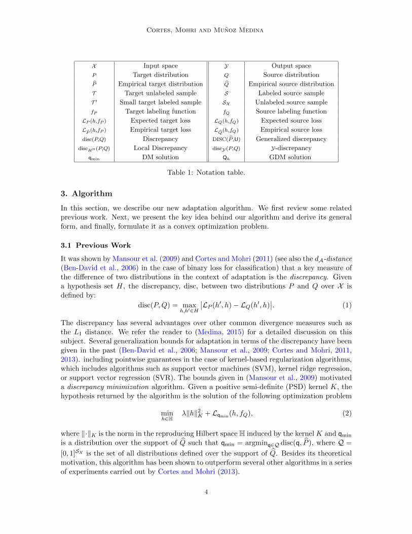
X Input space Y Output space

P Target distribution Q Source distribution

P Empirical target distribution Q Empirical source distribution

T Target unlabeled sample S Labeled source sample

T ′ Small target labeled sample SX Unlabeled source sample

fP Target labeling function fQ Source labeling function

LP (h,fP ) Expected target loss LQ(h,fQ) Expected source loss

LP

(h,fP ) Empirical target loss LQ

(h,fQ) Empirical source loss

disc(P,Q) Discrepancy DISC(P ,U) Generalized discrepancy

discH′′ (P,Q) Local Discrepancy discY (P,Q) Y-discrepancy

qmin DM solution Qh GDM solution

Table 1: Notation table.

3. Algorithm

In this section, we describe our new adaptation algorithm. We first review some relatedprevious work. Next, we present the key idea behind our algorithm and derive its generalform, and finally, formulate it as a convex optimization problem.

3.1 Previous Work

It was shown by Mansour et al. (2009) and Cortes and Mohri (2011) (see also the dA-distance(Ben-David et al., 2006) in the case of binary loss for classification) that a key measure ofthe difference of two distributions in the context of adaptation is the discrepancy. Givena hypothesis set H, the discrepancy, disc, between two distributions P and Q over X isdefined by:

disc(P,Q) = maxh,h′∈H

∣∣LP (h′, h)− LQ(h′, h)∣∣. (1)

The discrepancy has several advantages over other common divergence measures such asthe L1 distance. We refer the reader to (Medina, 2015) for a detailed discussion on thissubject. Several generalization bounds for adaptation in terms of the discrepancy have beengiven in the past (Ben-David et al., 2006; Mansour et al., 2009; Cortes and Mohri, 2011,2013). including pointwise guarantees in the case of kernel-based regularization algorithms,which includes algorithms such as support vector machines (SVM), kernel ridge regression,or support vector regression (SVR). The bounds given in (Mansour et al., 2009) motivateda discrepancy minimization algorithm. Given a positive semi-definite (PSD) kernel K, thehypothesis returned by the algorithm is the solution of the following optimization problem

minh∈H

λ‖h‖2K + Lqmin(h, fQ), (2)

where ‖·‖K is the norm in the reproducing Hilbert space H induced by the kernel K and qmin

is a distribution over the support of Q such that qmin = argminq∈Q disc(q, P ), where Q =

[0, 1]SX is the set of all distributions defined over the support of Q. Besides its theoreticalmotivation, this algorithm has been shown to outperform several other algorithms in a seriesof experiments carried out by Cortes and Mohri (2013).

4


Observe that, by definition, the objective function optimized by qmin corresponds to amaximum over all pairs of hypotheses. But, the maximizing pair of hypotheses may not beamong the candidates ever considered by the learning algorithm. Thus, a learning algorithmbased on discrepancy minimization tends to be too conservative.

3.2 Main Idea

From here on we assume the algorithm selected by the learner is an instance of a regu-larized risk minimization algorithm over the Hilbert space H induced by a PSD kernel K.With knowledge of the target labels, these algorithms return a hypothesis h∗ solution ofminh∈H F (h) where

F (h) = λ‖h‖2K + LP

(h, fP ), (3)

where λ ≥ 0 is a regularization parameter. Thus, h∗ can be viewed as the ideal hypothesis.

In view of that, we can formulate our objective, in the presence of a domain adaptationproblem, as that of finding a hypothesis h whose loss LP (h, fP ) with respect to the targetdomain is as close as possible to LP (h∗, fP ). To do so, we will seek in fact a hypothesis hthat is as close as possible to h∗, which would imply the closeness of the losses with respectto the target domains. We do not have access to fP and can only access the labels ofthe training sample S. Thus, we must resort to using in our objective function, instead ofLP

(h, fP ), a reweighted empirical loss over the training sample S. The main idea behind ouralgorithm is to define, for any h ∈ H, a reweighting function Qh : SX = {x1, . . . , xm} → Rsuch that the objective function G defined for all h ∈ H by

G(h) = λ‖h‖2K + LQh(h, fQ) (4)

is uniformly close to F , thereby resulting in close minimizers. Since the first term of (3)and (4) coincide, the idea consists equivalently of seeking Qh such that LQh(h, fQ) andLP

(h, fP ) be as close as possible. Observe that this departs from the standard reweightingmethods: instead of reweighting the training sample with some fixed set of weights, weallow the weights to vary as a function of the hypothesis h. Note that we have furtherrelaxed the condition commonly adopted by reweighting techniques that the weights mustbe non-negative and sum to one.

Of course, searching for Qh to directly minimize |LQh(h, fQ)−LP

(h, fP )| is in general notpossible since we do not have access to fP , but it is instructive to consider the imaginarycase where the average loss L

P(h, fP ) is known to us for any h ∈ H. Qh could then be

determined via

Qh = argminq∈F(SX ,R)

|Lq(h, fQ)− LP

(h, fP )|, (5)

where F(SX ,R) is the set of real-valued functions defined over SX . For any h, we can in factselect Qh such that LQh(h, fQ) = L

P(h, fP ) since Lq(h, fQ) is a linear function of q. Thus,

the optimization problem (5) reduces to solving a simple linear equation. With this choice ofQh, the objective functions F and G coincide and by minimizing G we can recover the idealsolution h∗. Note that, in general, the DM algorithm could not recover that ideal solution.Even a finer discrepancy minimization algorithm exploiting the knowledge of L

P(h, fP ) for

all h and seeking a distribution q′min minimizing maxh∈H |Lq(h, fQ)−LP

(h, fP )| could not,

5


in general, recover the ideal solution since we could not have Lq′min(h, fQ) = L

P(h, fP ) for

all h ∈ H.Of course, L

P(h, fP ) is not accessible since the sample T is unlabeled. Instead, we will

consider a non-empty convex set of candidate hypotheses H ′′ ⊆ H that could contain agood approximation of fP . Using H ′′ as a set of surrogate labeling functions leads to thefollowing definition of Qh instead of (5):

Qh = argminq∈F(SX ,R)

maxh′′∈H′′

|Lq(h, fQ)− LP

(h, h′′)|. (6)

The choice of the subset H ′′ is of course key. Our choice will be based on the theoreticalanalysis of Section 4. Nevertheless, we now present the formulation of the optimizationproblem for an arbitrary choice of the convex subset H ′′.

Proposition 1 For any h ∈ H, let Qh be defined by (6). Then, the following identity holdsfor any h ∈ H:

LQh(h, fQ) =1

2

(maxh′′∈H′′

LP

(h, h′′) + minh′′∈H′′

LP

(h, h′′)).

Proof For any h ∈ H, the equation Lq(h, fQ) = l with l ∈ R admits a solution q ∈F(SX ,R). Thus, {Lq(h, fQ) : q ∈ F(SX ,R)} = R and for any h ∈ H, we can write

LQh(h, fQ) = argminl∈{Lq(h,fQ) : q∈F(SX ,R)}


|l − LP

(h, h′′)|

= argminl∈R


|l − LP

(h, h′′)|

= argminl∈R


max{LP

(h, h′′)− l, l − LP

(h, h′′)}

= argminl∈R

max{


LP

(h, h′′)− l, l − minh′′∈H′′

LP

(h, h′′)}

=1

2


LP

(h, h′′) + minh′′∈H′′

LP

(h, h′′)),

since the minimizing l is obtained for maxh′′∈H′′

LP

(h, h′′)− l= l − minh′′∈H′′

LP

(h, h′′).

In view of this proposition, with our choice of Qh based on (6), the objective functionG of our algorithm (4) can be equivalently written for all h ∈ H as follows:

G(h) = λ‖h‖2K +1

2


LP

(h, h′′) + minh′′∈H′′

LP

(h, h′′)). (7)

Using the fact the LP

is a jointly convex function, it is easy to show (see for instance Boydand Vandenberghe, 2004) that G is in fact a convex function too.

4. Learning Guarantees

Here, we present two different types of guarantees: a tight learning bound based on theRademacher complexity and a pointwise bound derived from a stability analysis. We furthershow that our algorithm is in fact minimizing this pointwise bound. As in previous work,we assume that the loss function L is µ-admissible.

6


Definition 2 A loss function L is µ-admissible if there exists µ > 0 such that the inequality

|L(h(x), y)− L(h′(x), y)| ≤ µ|h(x)− h′(x)| (8)

holds for all (x, y) ∈ X × Y and h′, h ∈ H.

The Lp losses commonly used in regression, p ≥ 1, verify this condition (see Ap-pendix C).

4.1 Rademacher Complexity Bounds

Definition 3 Let Z be any set and G be a family of functions mapping Z to R. Givena sample S = {z1, . . . , zn} ⊂ Z, the empirical Rademacher complexity of G is denoted byRS(G) and defined by

RS(G) =1

nEσ

[supg∈G

n∑

i=1

σig(zi)

],

where σis, called Rademacher variables, are independent random variables distributed ac-cording to the uniform distribution over {−1, 1}. The Rademacher complexity of G is definedas

Rn(G) = ES

[RS(G)

].

Our first generalization bound is given in terms of the Y-discrepancy, which is a gen-eralization of the discrepancy distance. The Y-discrepancy was first introduced by Mohriand Munoz (2012) in the context of learning with drifting distributions.

Definition 4 The Y-discrepancy between two domains (P, fP ) and (Q, fQ) is defined by

discY(P,Q) = suph∈H

∣∣LQ(h, fQ)− LP (h, fP )∣∣.

Note that the definition depends on the labeling functions fP and fQ. We do not explicitlyindicate that dependency for the sake of simplicity of the notation.

We follow the analysis of (Mohri and Munoz, 2012) to derive the following tight gener-alization bounds based on the notion of Y-discrepancy.

Proposition 5 Let HQ and HP be the families of functions defined as follows: HQ :={x 7→ L(h(x), fQ(x)) : h ∈ H} and HP := {x 7→ L(h(x), fP (x)) : h ∈ H}. Define MQ andMP as MQ = supx∈X ,h∈H L(h(x), fQ(x)) and MP = supx∈X ,h∈H L(h(x), fP (x)). Then, forany δ > 0,

1. with probability at least 1 − δ over the choice of a labeled sample S of size m, the fol-lowing inequality holds for all h ∈ H:

LP (h, fP ) ≤ LQ

(h, fQ) + discY(P,Q) + 2Rm(HQ) +MQ

√log(1

δ )

2m; (9)

2. with probability at least 1 − δ over the choice of a sample T of size n, the followinginequality holds for all h ∈ H and any distribution q over a sample SX :

LP (h, fP ) ≤ Lq(h, fQ) + discY(P , q) + 2Rn(HP ) +MP

√log(1

δ )

2n. (10)

7


Proof Let Φ(S) denote suph∈H LQ(h, fQ)− LP (h, fP ). Changing one point in S changes

Φ(S) by at mostMQ

m . Thus, by McDiarmid’s inequality, we have P(Φ(S)−E[Φ(S)] > ε

)≤

e− 2mε2

M2Q . Therefore, for any δ > 0, with probability at least 1− δ, the following holds for all

h ∈ H:

LP (h, fP ) ≤ LQ

(h, fQ) + E[Φ(S)] +MQ

√log(1

δ )

2m.

Next, we can bound E[Φ(S)] as follows:

E[Φ(S)] = E

[suph∈HLQ

(h, fQ)− LP (h, fP )

]

≤ E

[suph∈HLQ

(h, fQ)− LQ(h, fQ)

]+ suph∈HLQ(h, fQ)− LP (h, fP )

≤ 2Rm(HQ) + discY(P,Q),

where the last inequality follows from a standard symmetrization inequality in terms of theRademacher complexity and the definition of discY(P,Q).

For the second bound we have, starting with a standard Rademacher complexity boundfor HP , for any δ > 0, with probability at least 1− δ, the following holds for all h ∈ H:

LP (h, fP ) ≤ LP

(h, fP ) + 2Rn(HP ) +MP

√log(1

δ )

2n

≤ Lq(h, fQ) + LP

(h, fP )− Lq(h, fQ) + 2Rn(HP ) +MP

√log(1

δ )

2n. (11)

Moreover, by definition LP

(h, fP )−Lq(h, fQ) ≤ discY(P , q) for any q. Replacing this boundin (11) yields the result.

Observe that these bounds are tight as a function of the divergence measure (discrep-ancy) we use: in the absence of adaptation, the following standard Rademacher complexitylearning bound holds:

LP

(h, fP ) ≤ LP

(h, fP ) + 2Rn(HP ) +MP

√log(1

δ )

2n.

Our second adaptation bound differs from this inequality only by the fact that LP

(h, fP ) is

replaced with Lq(h, fQ) + discY(P , q). But, by definition of Y-discrepancy, there exists an

h ∈ H such that |LP

(h, fP ) − Lq(h, fQ)| = discY(P , q). A similar analysis shows that ourfirst bound is also tight.

Given a labeled sample S from the source domain, Proposition 5 suggests choosing adistribution q with support SX that minimizes the right-hand side of (10). However, thequantity discY(P , q) depends, by definition, on the unknown labels from the target domainand therefore cannot be minimized. Thus, we will instead upper bound the Y-discrepancyin terms of quantities that can be estimated.

8


Let A(H) denote the set of all functions U : h 7→ Uh mapping H to F(SX ,R) such thatfor all h ∈ H, h 7→ LUh(h, fQ) is a convex function. Thus, for any h ∈ H, Uh is a reweightingfunction defined over SX . A(H) contains all constant functions U such that Uh = q for allh ∈ H, where q is a distribution over SX . We will abuse the notation and denote thisfunctions also by q. By Proposition 1, A(H) also includes the function Q : h→ Qh used byour algorithm.

Definition 6 (Generalized discrepancy) For any U ∈ A(H), the generalized discrep-ancy between P and U is denoted by DISC(P ,U) and is defined by

DISC(P ,U) = suph∈H,h′′∈H′′

|LP

(h, h′′)− LUh(h, fQ)|. (12)

We also denote by d1(fP , H′′) the L1 distance of fP to H ′′:

d1(fP , H′′) = min

h0∈H′′EP|h0(x)− fP (x)|. (13)

The following theorem gives an upper bound on the Y-discrepancy in terms of the general-ized discrepancy and d1(fP , H

′′).

Proposition 7 For any distribution q over SX and any set H ′′, the following inequalityholds:

discY(P , q) ≤ DISC(P , q) + µd1(fP , H′′).

Proof Let h0 ∈ H ′′, by the triangle inequality, we can write

discY(P , q) = suph∈H|Lq(h, fQ)− L

P(h, fP )|

≤ suph∈H|Lq(h, fQ)− L

P(h, h0)|+ sup

h∈H|LP

(h, h0)− LP

(h, fP )|

≤ suph∈H


|Lq(h, fQ)− LP

(h, h′′)|+ suph∈H|LP

(h, h0)− LP

(h, fP )|.

The hypothesis h0 will later be chosen to minimize the distance of fP to H ′′. By theµ-admissibility of the loss, the last term can be bounded as follows:

suph∈H|LP

(h, h0)− LP

(h, fP )| ≤ µEP|fP (x)− h0(x)|.

Using this inequality and minimizing over h0 ∈ H ′′ yields:

discY(P , q) ≤ suph∈H


|Lq(h, fQ)− LP

(h, h′′)|+ µd1(fP , H′′)

= DISC(P , q) + µd1(fP , H′′),

which completes the proof.

We can also bound the Y-discrepancy in terms of the discrepancy measure and thefollowing measure of the difference of the source and target labeling functions:

ηH(fP , fQ) = minh0∈H

(max

x∈supp(P )|fP (x)− h0(x)|+ max

x∈supp(Q)|fQ(x)− h0(x)|

).

9


Proposition 8 The following inequality holds for all distributions q over SX :

discY(P , q) ≤ disc(P , q) + µ ηH(fP , fQ).

Proof By the triangle inequality and the µ-admissibility of the loss, the following inequalityholds for all h0 ∈ H:

discY(P , q)

= suph∈H|Lq(h, fQ)− L

P(h, fP )|

≤ suph∈H

(|LP

(h, h0)− LP

(h, fP )|+ |Lq(h, fQ)− Lq(h, h0)|)

+ suph∈H|Lq(h, h0)− L

P(h, h0)|

≤ µ(

supx∈supp(P )

|h0(x)− fP (x)|] + supx∈supp(Q)

[|fQ(x)− h0(x)|])

+ disc(P , q).

Minimizing over all h0 ∈ H gives discY(P , q) ≤ µ ηH(fP , fQ) + disc(P , q) and completes theproof.

The following learning guarantees are immediate consequences of Propositions 5, 7 and8.

Corollary 9 Let H ′′ ⊂ H be a convex set and q a distribution over SX . Then, for anyδ > 0, each of the following inequalities holds with probability at least 1− δ for all h ∈ H:

LP (h, fP ) ≤ Lq(h, fQ) + DISC(P , q) + µd1(fP , H′′) + 2Rn(HP ) +MP

√log(1

δ )

2n, (14)

LP (h, fP ) ≤ Lq(h, fQ) + disc(P , q) + µ ηH(fP , fQ) + 2Rn(HP ) +MP

√log(1

δ )

2n. (15)

In general, the bounds (14) and (15) are not comparable. However, when L is an LPloss for some p ≥ 1, we can show the existence of a set H ′′ for which (14) is a tighter boundthan (15). The result is expressed in terms of the local discrepancy defined by:

discH′′(P , q) = suph∈H,h′′∈H′′

|LP

(h, h′′)− Lq(h, h′′)|,

which is a finer measure than the standard discrepancy for which the supremum is definedover a pair of hypotheses both in H ⊇ H ′′.

Theorem 10 Let L be the LP loss for some p ≥ 1. Let H := {B(r) : r ≥ 0} be a set of allballs B(r) = {h′′ ∈ H|Lq(h′′, fQ) ≤ rp}. Then, for any distribution q over SX , there existsH ′′ ∈ H such that the following holds:

DISC(P , q) + µd1(fP , H′′) ≤ discH′′(P , q) + µ ηH(fP , fQ).

10


Proof Fix a distribution q over SX . Let h∗0 be an element of argminh0∈H(LP

(h0, fP )1p +

Lq(h0, fQ)1p). Choose H ′′ ∈ H as H ′′ = {h′′ ∈ H|Lq(h′′, fQ) ≤ rp} with r = Lq(h∗0, fQ)

1p .

Then, by definition, h∗0 is in H ′′. For the Lp loss, it is not hard to show that for all h, h′′ ∈ H,

|Lq(h, h′′) − Lq(h, fQ)| ≤ µ[Lq(h′′, fQ)]1p (see Appendix C). In view of this inequality, we

can write:

DISC(P , q) = suph∈H,h′′∈H′′

|LP

(h, h′′)− Lq(h, fQ)|

≤ suph∈H,h′′∈H′′

|LP

(h, h′′)− Lq(h, h′′)|+ suph∈H,h′′∈H′′

|Lq(h, h′′)− Lq(h, fQ)|

≤ discH′′(P , q) + maxh′′∈H′′

µ[Lq(h′′, fQ)]1p

= discH′′(P , q) + µr = discH′′(P , q) + µLq(h∗0, fQ)1p .

Using this inequality, Jensen’s inequality, and the fact that h∗0 is in H ′′, we can write

µd1(fP , H′′) + DISC(P , q)

≤ µ minh0∈H′′

Ex∈P

[|fP (x)− h0(x)|] + µLq(h∗0, fQ)1p + discH′′(P , q)

≤ µ minh0∈H′′

Ex∈P

[|fP (x)− h0(x)|p]1p + µLq(h∗0, fQ)

1p + discH′′(P , q)

≤ µLP

(h∗0, fP )1p + µLq(h∗0, fQ)

1p + discH′′(P , q).

Moreover, by definition of h∗0 the last expression is equal to

µ minh0∈H

(LP

(h0, fP )1p + Lq(h0, fQ)

1p

)+ discH′′(P , q)

≤ µ minh0∈H

(max

x∈supp(P )|fP (x)− h0(x)|+ max

x∈supp(Q)|fQ(x)− h0(x)|

)+ discH′′(P , q)

= µ ηH(fP , fQ) + discH′′(P , q).

which concludes the proof.

Theorem 10 shows that the generalized discrepancy can provide a finer measure of thedifference between two domains for some choices of H ′′. Therefore, for a good choice of H ′′,an algorithm minimizing the right-hand side of (14) would benefit from better theoreticalguarantees than the DM algorithm. However, the optimization problem defined by (14)is not jointly convex in q and h. Instead, we propose to first minimize the generalizeddiscrepancy and then use this reweighting function as input to our learning algorithm.Further motivation for this two-stage algorithm is given in the following section.

4.2 Pointwise Guarantees

Similar to the guarantee presented by Cortes and Mohri (2013), we will seek to bound thedifference between an ideal solution h∗ and the solution obtained by our algorithm. Webegin by stating the following bound motivating the DM algorithm.

11


Theorem 11 (Cortes and Mohri, 2013) Let q be an arbitrary distribution over SX andlet h∗ and hq be the hypotheses minimizing λ‖h‖2K + L

P(h, fP ) and λ‖h‖2K + Lq(h, fQ)

respectively. Then, the following inequality holds:

λ‖h∗ − hq‖2K ≤ µ ηH(fP , fQ) + disc(P , q). (16)

Notice that the solution of DM minimizes the right-hand side of (16), that is disc(P , q).The following theorem provides an analogous bound for our algorithm.

Theorem 12 Let U be an arbitrary element of A(H) and let h∗ and hU be the hypothesesminimizing λ‖h‖2K + L

P(h, fP ) and λ‖h‖2K + LUh(h, fQ) respectively. Then, the following

inequality holds for any convex set H ′′ ⊆ H:

λ‖h∗ − hU‖2K ≤ µd1(fP , H′′) + DISC(P ,U). (17)

Proof Fix U ∈ A(H) and let GP

denote h 7→ LP

(h, fP ) and GU the function h 7→LUh(h, fQ). Since h 7→ λ‖h‖2K + G

P(h) is convex and differentiable and since h∗ is its

minimizer, the gradient is zero at h∗, that is 2λh∗ = −∇GP

(h∗). Similarly, since h 7→λ‖h‖2K+GU(h) is convex, it admits a sub-differential at any h ∈ H. Since hU is a minimizer,its sub-differential at hU must contain 0. Thus, there exists a sub-gradient g0 ∈ ∂GU(hU)such that 2λhU = −g0, where ∂GU(hU) denotes the sub-differential of GU at hU. Usingthese two equalities we can write

2λ‖h∗ − hU‖2K = 〈h∗ − hU, g0 −∇GP (h∗)〉 = 〈g0, h∗ − hU〉 − 〈∇GP (h∗), h∗ − hU〉

≤ GU(h∗)−GU(hU) +GP

(hU)−GP

(h∗)

= LP

(hU, fP )− LUh(hU, fQ) + LUh(h∗, fQ)− LP

(h∗, fP )

≤ 2 suph∈H|LP

(h, fP )− LUh(h, fQ)|,

where we used for the first inequality the convexity of GU combined with the sub-gradientproperty of g0 ∈ ∂GU(hU), and the convexity of G

P. For any h ∈ H, using the µ-

admissibility of the loss, we can upper bound the operand of the max operator as follows:

|LP

(h, fP )− LUh(h, fQ)| ≤ |LP

(h, fP )− LP

(h, h0)|+ |LP

(h, h0)− LUh(h, fQ)|≤ µ E

x∼P|fP (x)− h0(x)|+ max

h′′∈H′′|LP

(h, h′′)− LUh(h, fQ)|,

where h0 is an arbitrary element of H ′′. Since this bound holds for all h0 ∈ H ′′, it followsimmediately that

λ‖h∗ − hU‖2K ≤ µ minh0∈H′′

EP|fP (x)− h0(x)|+ sup

h∈Hmaxh′′∈H′′

|LP

(h, h′′)− LUh(h, fQ)|,


Note that our choice of Q : h 7→ Qh minimizes the right-hand side of (17) among allfunctions U ∈ A(H) since, for any U, we can write

DISC(P ,U)= suph∈H


|LP

(h, h′′)−LUh(h, fQ)|≥ suph∈H

minq∈F(SX )


|LP

(h, h′′)−Lq(h, fQ)|

= suph∈H


|LP

(h, h′′)− LQh(h, fQ)| = DISC(P ,Q).

12


Thus, in view of Theorem 10, for any constant function U ∈ A(H) with Uh = q for somefixed distribution q over SX , the right-hand side of the bound of Theorem 11 is lowerbounded by the right-hand side of the bound of Theorem 12, since the local discrepancy isa finer quantity than the discrepancy: discH′′(P , q) ≤ disc(P , q). Thus, as expected fromthe discussion after Theorem 10, our algorithm benefits from a more favorable guaranteethan the DM algorithm for some particular choices of H ′′, especially since, our choice of Qis based on the minimization over all elements in A(H) and not just the subset of constantfunctions mapping to a distribution. The following pointwise guarantee follows directlyfrom Theorem 12.

Corollary 13 Let h∗ be a minimizer of λ‖h‖2K+LP

(h, fP ) and hQ a minimizer of λ‖h‖2K+LQh(h, fQ). Then, the following holds for any convex set H ′′ ⊆ H and for all (x, y) ∈ X×Y:

|L(hQ(x), y)− L(h∗(x), y)| ≤ µR

√µd1(fP , H ′′) + DISC(P ,Q)

λ, (18)

where R2 = supx∈X K(x, x).

Proof By the µ-admissibility of the loss, the reproducing property of H, and the Cauchy-Schwarz inequality, the following holds for all x ∈ X and y ∈ Y:

|L(hQ(x), y)− L(h∗(x), y)| ≤ µ|hQ(x)− h∗(x)|= µ|〈hQ − h∗,K(x, ·)〉K |

≤ µ‖hQ − h∗‖K√K(x, x) ≤ R‖hQ − h∗‖K .

Upper bounding ‖hQ − h∗‖K using Theorem 12 and using the fact that Q : h → Qh is aminimizer of the bound over all choices of U ∈ A(H) yields the desired result.

The pointwise loss guarantee just presented can be directly used to bound the differenceof the expected loss of h∗ and hQ in terms of the same upper bounds, e.g.,

LP (hQ, fP ) ≤ LP (h∗, fP ) + µR

√µd1(fP , H ′′) + DISC(P ,Q)

λ. (19)

Similarly, Theorem 10 directly implies the following Corollary.

Corollary 14 Let h∗ be a minimizer of λ‖h‖2K+LP

(h, fP ) and hQ a minimizer of λ‖h‖2K+LQh(h, fQ). Let supx∈X K(x, x) = R2. Then, there exists a choice of H ′′ ∈ H for which thefollowing inequality holds uniformly over over (x, y) ∈ X × Y:

|L(hQ(x), y)− L(h∗(x), y)| ≤ µR

√µηH(fP , fQ)+discH′′(P , qmin)

λ,

where qmin is the solution of the DM algorithm.

13


The choice of the set H ′′ defining our algorithm is strongly motivated by the theoreticalresults of this section. In view of Theorem 10, we restrict our choice of H ′′ to the family H,parametrized only by the radius r. Since the generalized discrepancy DISC is a function ofthe set H ′′ which in turn depends only on r, the radius r is chosen to minimize (19). Thiscan be done by using as a validation set a small amount of labeled data from the targetdomain which is typically available in practice. In particular, as the size of the unlabeledsample T ′ increases, our estimate of the optimal radius r becomes more accurate. Weprovide a detailed description of our algorithm’s implementation in Section 5.

4.3 Comparison against Other Learning Bounds

We now compare the learning bounds just derived for our algorithm with those of somecommon reweighting techniques. In particular, we compare our bounds with those of Corteset al. (2008) for the KMM algorithm. A similar comparison however can be derived for otheralgorithms based on importance weighting such as KLIEP or uLSIF.

Assume P and Q admit densities p and q respectively. For every x ∈ X we denote byβ(x) = p(x)

q(x) the importance ratio and by β = β∣∣SX

its restriction to SX . We also let β bethe solution to the optimization problem solved by the KMM algorithm. Let hβ denote thesolution to

minh∈H

λ‖h‖2 + Lβ(h, fQ), (20)

and hβ

be the solution to

minh∈H

λ‖h‖2 + Lβ(h, fQ). (21)

The following proposition due to Cortes et al. (2008) relates the error of these hypotheses.The proposition requires the kernel K to be a strictly positive definite universal kernel, withGram matrix K given by Kij = K(xi, xj).

Proposition 15 Assume L(h(x), y) ≤ 1 for all (x, y) ∈ X ×Y, h ∈ H. For any δ > 0, withprobability at least 1− δ we have:

|LP (hβ, fP )− LP (hβ, fP )| ≤ µ2R2λ

12max(K)

λ

( εB′√m

+κ1/2

λ1/2min(K)

√B′2

m+

1

n

(1 +

√2 log

2

δ

)), (22)

where ε and B′ are the hyperparameters defining the KMM algorithm and λmax(K), λmin(K)denote the largest and smallest eigenvalues of K respectively.

This bound and the one obtained in (19) are of course not comparable since the depen-dence on µ,R and λ is different. In some cases this dependency can be more favorable in(22) whereas for other values of these parameters (19) provides a better bound. Moreover,(22) depends on the condition number of K which can become really large in practice.However, the most important difference between these bounds is that (19) is given in termsof the ideal hypothesis h∗ while (22) is given in terms of hβ, which, in view of the results ofCortes et al. (2010) is not guaranteed to have a good performance on the target distribution.Therefore (22) does not, in general, provide an informative bound.

14


4.4 Scenario of Additional Labeled Data

Here, we consider a rather common scenario in practice where, in addition to the labeledsample S drawn from the source domain and the unlabeled sample T from the targetdomain, the learner receives a small amount of labeled data from the target domain T ′ =((x′′1, y

′′1), . . . , (x′′s , y

′′s )) ∈ (X × Y)s. This sample is typically too small to be used solely to

train an algorithm and achieve a good performance. However, it can be useful in at leasttwo ways that we discuss here.

One important benefit of T ′ is to serve as a validation set to determine the parameterr that defines the convex set H ′′ used by our algorithm. The sample T ′ can also be usedto enhance the discrepancy minimization algorithm as we now show. Let P ′ denote theempirical distribution associated with T ′. To take advantage of T ′, the DM algorithm canbe trained on the sample of size (m+s) obtained by combining S and T ′, which correspondsto the new empirical distribution Q′ = m

m+sQ+ sm+s P

′. Note that for a fixed value m and

large values of s, Q′ essentially ignores the points from the source distribution Q, whichcorresponds to the standard supervised learning scenario in the absence of adaptation.Let q′min denote the discrepancy minimization solution when using Q′. Since supp(Q′) ⊇supp(Q), the discrepancy using q′min is a lower bound on the discrepancy using qmin:

disc(q′min, P ) = minsupp(q)⊆supp(Q′)

disc(P , q) ≤ minsupp(q)⊆supp(Q)

disc(P , q) = disc(qmin, P ).

5. Optimization Solution

As shown in Section 3.2, the function G defining our algorithm is convex and the prob-lem of minimizing the expression (7) is a convex optimization problem. Nevertheless,the problem is not straightforward to solve, in particular because evaluating a term likemaxh′′∈H′′ LP (h, h′′) that it contains requires solving a non-convex optimization problem.Here, we present an exact solution in the case of the L2 loss by solving a semi-definiteprogramming (SDP) problem.

5.1 SDP Formulation

As discussed in Section 4, the choice of H ′′ is a key component of our algorithm. In viewof Corollary 14, we will consider the set H ′′ = {h′′ | Lqmin(h′′, fQ) ≤ r2}. Equivalently, as aresult of the reproducing property of H and the representer theorem, H ′′ may be defined as{a ∈ Rm|

∑mj=1 qmin(xj)(

∑mi=1 aiqmin(xi)

1/2K(xi, xj)− yj)2 ≤ r2}. Also by the representer

theorem, the solution to (7) will be of the form h = n−1/2∑n

i=1 biK(x′i, ·). Therefore,

given normalized kernel matrices Kt, Ks, Kst defined respectively as Kijt = n−1K(x′i, x

′j),

Kijs = qmin(xi)

1/2qmin(xj)1/2K(xi, xj) and Kij

st = n−1/2qmin(xj)1/2K(x′i, xj), problem (7) is

equivalent to

minb∈Rn

λb>Ktb +1

2

(maxa∈Rm

‖Ksa−y‖2≤r2‖Ksta−Ktb‖2 + min

a∈Rm‖Ksa−y‖2≤r2

‖Ksta−Ktb‖2), (23)

where y = (qmin(x1)1/2y1, . . . , qmin(xm)1/2ym) is the vector of normalized labels.

15


h0

g1(h) = 0

g2(h) = 0

h0 + �⇤bh

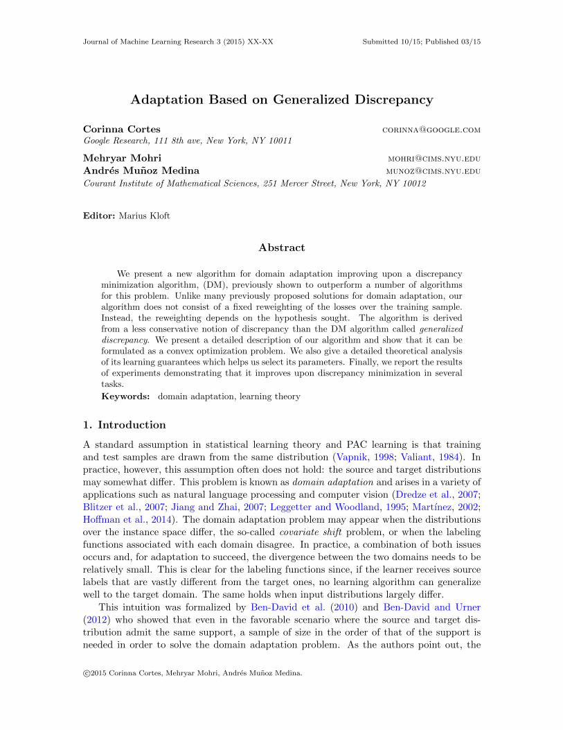
Friday, February 7, 2014

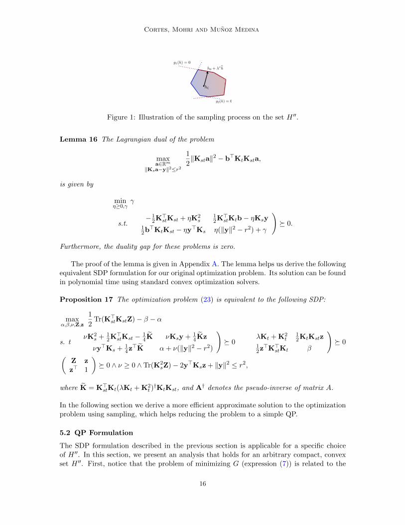
Figure 1: Illustration of the sampling process on the set H ′′.

Lemma 16 The Lagrangian dual of the problem

maxa∈Rm

‖Ksa−y‖2≤r2

1

2‖Ksta‖2 − b>KtKsta,

is given by

minη≥0,γ

γ

s.t.

(−1

2K>stKst + ηK2s

12K>stKtb− ηKsy

12b>KtKst − ηy>Ks η(‖y‖2 − r2) + γ

)� 0.

Furthermore, the duality gap for these problems is zero.

The proof of the lemma is given in Appendix A. The lemma helps us derive the followingequivalent SDP formulation for our original optimization problem. Its solution can be foundin polynomial time using standard convex optimization solvers.

Proposition 17 The optimization problem (23) is equivalent to the following SDP:

maxα,β,ν,Z,z

1

2Tr(K>stKstZ)− β − α

s. t

(νK2

s + 12K>stKst − 1

4K νKsy + 14Kz

νy>Ks + 14z>K α+ ν(‖y‖2 − r2)

)� 0

(λKt + K2

t12KtKstz

12z>K>stKt β

)� 0

(Z zz> 1

)� 0 ∧ ν ≥ 0 ∧ Tr(K2

sZ)− 2y>Ksz + ‖y‖2 ≤ r2,

where K = K>stKt(λKt + K2t )†KtKst, and A† denotes the pseudo-inverse of matrix A.

In the following section we derive a more efficient approximate solution to the optimizationproblem using sampling, which helps reducing the problem to a simple QP.

5.2 QP Formulation

The SDP formulation described in the previous section is applicable for a specific choiceof H ′′. In this section, we present an analysis that holds for an arbitrary compact, convexset H ′′. First, notice that the problem of minimizing G (expression (7)) is related to the

16


minimum enclosing ball (MEB) problem. For a set D ⊆ Rd, the MEB problem is definedas follows:

minu∈Rd

maxv∈D‖u− v‖2.

Omitting the regularization and the min term from (7) leads to a problem similar to theMEB. Thus, we could benefit from the extensive literature and algorithmic study availablefor this problem (Kumar et al., 2003; Schonherr, 2002; Yildirim, 2008). However, to thebest of our knowledge, there is currently no solution available to this problem in the case ofan infinite set D, as in the case of our problem. Instead, we present a solution for solvingan approximation of (7) based on sampling.

Let {h1, . . . , hk} be a set of hypotheses on the boundary of H ′′, ∂H ′′ and let C =C(h1, . . . , hk) denote their convex hull. The following is the sampling-based approximationof (7) that we consider:

minh∈H

λ‖h‖2K +1

2maxi=1,...,k

LP

(h, hi) +1

2minh′∈CLP

(h, h′). (24)

Proposition 18 Let Y = (Yij) ∈ Rn×k be the matrix defined by Yij = n−1/2hj(x′i) and

y′ = (y′1, . . . , y′k)> ∈ Rk the vector defined by y′i = n−1

∑nj=1 hi(x

′j)

2. Then, the dualproblem of (24) is given by

maxα,γ,β

−(Yα+

γ

2

)>Kt

(λI +

1

2Kt

)−1(Yα+

γ

2

)− 1

2γ>KtK

†tγ +α>y′ − β (25)

s.t. 1>α =1

2, 1β ≥ −Y>γ, α ≥ 0,

where 1 is the vector in Rk with all components equal to 1. Furthermore, the solution hof (24) can be recovered from a solution (α,γ, β) of (25) by ∀x, h(x) =

∑ni=1 aiK(xi, x),

where a =(λI + 1

2Kt)−1(Yα+ 1

2γ).

The proof of the proposition is given in Appendix B. The result shows that, given afinite sample h1, . . . , hk on the boundary of H ′′, (24) is in fact equivalent to a standard QP.Hence, a solution can be found efficiently with one of the many off-the-shelf algorithms forquadratic programming.

We now describe the process of sampling from the boundary of the set H ′′, which isa necessary step for defining problem (24). We consider compact sets of the form H ′′ :={h′′ ∈ H | gi(h′′) ≤ 0}, where the functions gi are continuous and convex. For instance, wecould consider the set H ′′ defined in the previous section. More generally, we can considera family of sets H ′′p = {h′′ ∈ H| |

∑mi=1 qmin(xi)|h(xi)− yi|p ≤ rp}.

Assume that there exists h0 satisfying gi(h0) < 0. Our sampling process is illustrated byFigure 1 and works as follows: pick a random direction h and define λi to be the minimalsolution to the system

(λ ≥ 0) ∧ (gi(h0 + λh) = 0).

Set λi =∞ if no solution is found and define λ∗ = mini λi. By the convexity and compact-ness of H ′′ we can guarantee that λ∗ < ∞. The hypothesis h = h0 + λ∗h satisfies h ∈ H ′′and gj(h) = 0 for j such that λj = λ∗. The latter is straightforward. To verify the former,

17


assume that gi(h0 + λ∗h) > 0 for some i. The continuity of gi would imply the existence ofλ′i with 0 < λ′i < λ∗ ≤ λi such that gi(h0 + λ′ih) = 0. This would contradict the choice of

λi, thus, the inequality gi(h0 + λ∗h) ≤ 0 must hold for all i.

Since a point h0 with gi(h0) < 0 can be obtained by solving a convex program andsolving the equations defining λi is, in general, simple, the process described provides anefficient way of sampling points from the convex set H ′′.

5.3 Implementation for the L2 Loss

We now describe how to fully implement our sampling-based algorithm for the case whereL is equal to the L2 loss. In view of the results of Section 4, we let H ′′ = {h′′|‖h′′‖K ≤Λ ∧ Lq(h′′, fQ) ≤ r2}. We first describe the steps needed to find a point h0 ∈ H ′′. LethΛ be such that ‖hΛ‖K = Λ and λr ∈ R+ be such that the solution hr to the optimizationproblem

minh∈H

λr‖h‖2 + Lq(h, fQ),

satisfies Lq(hr, fQ) = r2. It is easy to verify that the existence of λr is guaranteed forminh∈H Lq(h, fQ) ≤ r2 ≤

∑mi=1 q(xi)y

2i . It is clear that the point h0 = 1

2(hr + hΛ) is inthe interior of H ′′. Of course, finding λr with the desired properties is not straightforward.However, since r is chosen via validation, we do not need to find λr as a function of r.Instead, we can simply select λr through validation too.

In order to complete the sampling process, we must have an efficient way of selecting arandom direction h. If H ⊂ Rd is a set of linear hypotheses, a direction h can be sampleduniformly by letting h = ξ

‖ξ‖ , where ξ is a standard Gaussian random variable in Rd. If His a subset of a RKHS, by the representer theorem, we only need to consider hypotheses ofthe form h =

∑mi=1 αiK(xi, ·). Therefore, we can sample a direction h =

∑mi=1 α

′iK(xi, ·),

where the vector α′ = (α′1, . . . , α′m) is drawn uniformly from the unit sphere in Rm. A full

implementation of our algorithm thus consists of the following steps:

• find the distribution qmin = argminq∈Q disc(q, P ). This can be done by using thesmooth approximation algorithm of Cortes and Mohri (2013);

• sample points from the set H ′′ using the sampling process described above;

• solve the QP introduced in Section 5.2.

Notice that our algorithm only requires solving a simple QP and therefore its complexityis the same as other adaptation algorithms such as KMM, KLIEP and DM.

6. Experiments

Here, we report the results of extensive comparisons between GDM and several other adap-tation algorithms which demonstrate the benefits of our algorithm. We use the implemen-tation described in the previous section. The source code for our algorithm as well as allother baselines described in this section can be found at http://cims.nyu.edu/~munoz.

6.1 Synthetic Data Set

To compare the performances of the GDM and DM algorithms, we considered the followingsynthetic one-dimensional task, which is similar to the one considered by Huang et al.

18

http://cims.nyu.edu/~munoz


●●

●

●●

●

●

●

●

●

●

●

●

●

●●

●

●

●

●

●●

●

●●

●

●

●

●●

●

●

●

●

●

●●

●● ●

●

●

●

●

●●

●

●●

●

●

●

●

● ●

●

●

●

●●

●

●

●

●

●

●

●

●

●

●

●●

●●

●●

●●

●

●

●

●

●●● ●

●●

●●

●

●

●

●

●

●

●

●

●

●

−0.2 0.0 0.2 0.4 0.6 0.8 1.0 1.2

−1.2

−0.8

−0.4

0.0

0.2

SourceTargetDMGDM

w

MSE

(a) (b)

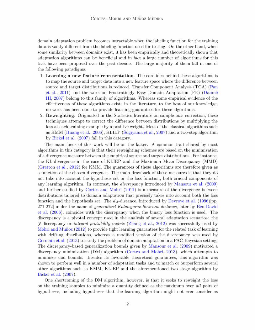
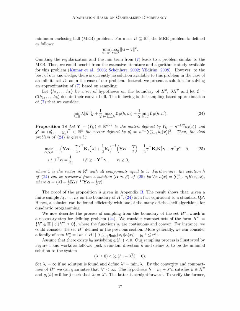
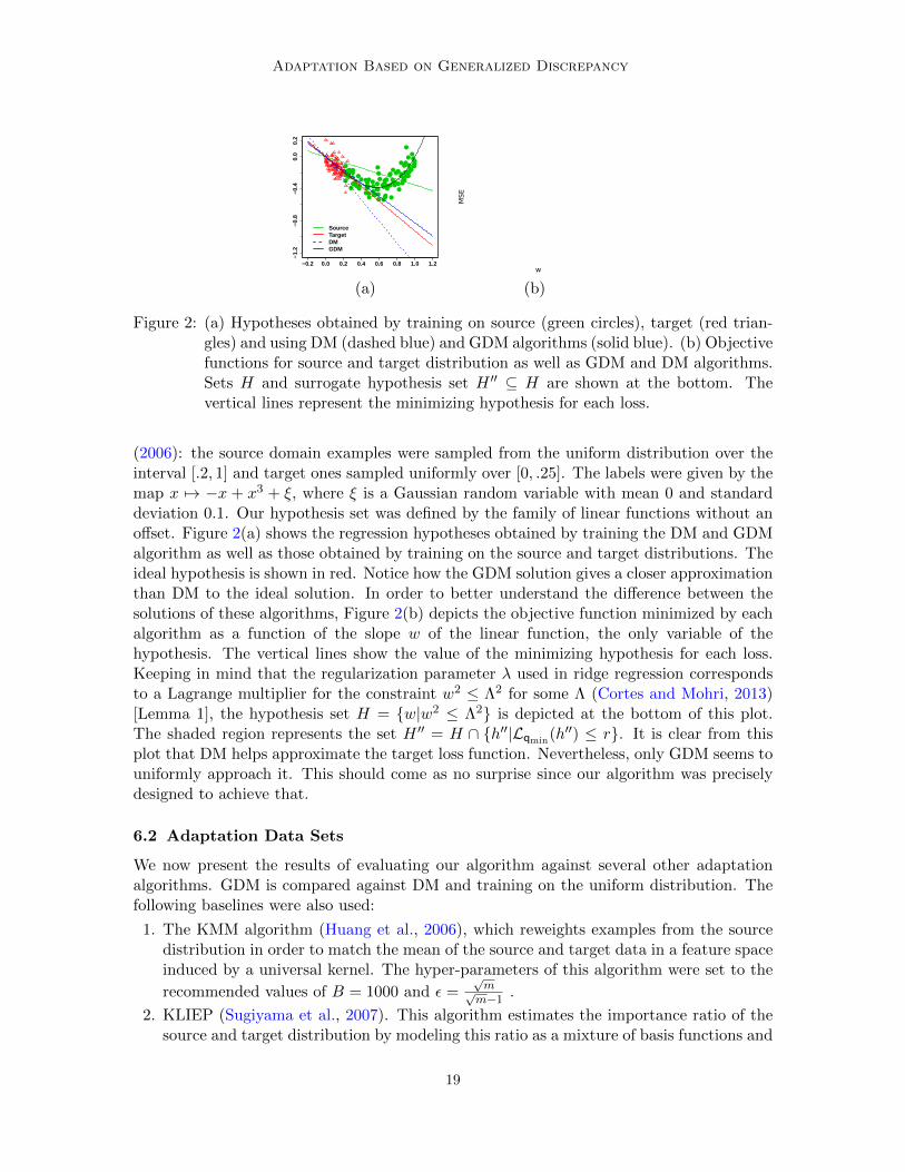
Figure 2: (a) Hypotheses obtained by training on source (green circles), target (red trian-gles) and using DM (dashed blue) and GDM algorithms (solid blue). (b) Objectivefunctions for source and target distribution as well as GDM and DM algorithms.Sets H and surrogate hypothesis set H ′′ ⊆ H are shown at the bottom. Thevertical lines represent the minimizing hypothesis for each loss.

(2006): the source domain examples were sampled from the uniform distribution over theinterval [.2, 1] and target ones sampled uniformly over [0, .25]. The labels were given by themap x 7→ −x + x3 + ξ, where ξ is a Gaussian random variable with mean 0 and standarddeviation 0.1. Our hypothesis set was defined by the family of linear functions without anoffset. Figure 2(a) shows the regression hypotheses obtained by training the DM and GDMalgorithm as well as those obtained by training on the source and target distributions. Theideal hypothesis is shown in red. Notice how the GDM solution gives a closer approximationthan DM to the ideal solution. In order to better understand the difference between thesolutions of these algorithms, Figure 2(b) depicts the objective function minimized by eachalgorithm as a function of the slope w of the linear function, the only variable of thehypothesis. The vertical lines show the value of the minimizing hypothesis for each loss.Keeping in mind that the regularization parameter λ used in ridge regression correspondsto a Lagrange multiplier for the constraint w2 ≤ Λ2 for some Λ (Cortes and Mohri, 2013)[Lemma 1], the hypothesis set H = {w|w2 ≤ Λ2} is depicted at the bottom of this plot.The shaded region represents the set H ′′ = H ∩ {h′′|Lqmin(h′′) ≤ r}. It is clear from thisplot that DM helps approximate the target loss function. Nevertheless, only GDM seems touniformly approach it. This should come as no surprise since our algorithm was preciselydesigned to achieve that.

6.2 Adaptation Data Sets

We now present the results of evaluating our algorithm against several other adaptationalgorithms. GDM is compared against DM and training on the uniform distribution. Thefollowing baselines were also used:

1. The KMM algorithm (Huang et al., 2006), which reweights examples from the sourcedistribution in order to match the mean of the source and target data in a feature spaceinduced by a universal kernel. The hyper-parameters of this algorithm were set to the

recommended values of B = 1000 and ε =√m√m−1

.

2. KLIEP (Sugiyama et al., 2007). This algorithm estimates the importance ratio of thesource and target distribution by modeling this ratio as a mixture of basis functions and

19


0.0

0.5

1.0

1.5

2.0

2.5

3.0

3.5

MSE

Source distribution: kin−8fh

0.0

0.5

1.0

1.5

2.0

2.5

3.0

3.5

0.0

0.5

1.0

1.5

2.0

2.5

3.0

3.5

0.0

0.5

1.0

1.5

2.0

2.5

3.0

3.5 GDM

DMUnifTargetKMMKLIEPFE

kin−8nm kin−8fm kin−8nh

0.0 0.5 1.0 1.5 2.0

0.2

0.4

0.6

0.8

1.0

0.0 0.5 1.0 1.5 2.0

0.2

0.4

0.6

0.8

1.0

DM

/GD

M

0.0 0.5 1.0 1.5 2.0

0.2

0.4

0.6

0.8

1.0

●

●

●

● ●

●

● ●

●

●

r Λ

● fh to nmfh to fmfh to nh

(a) (b)

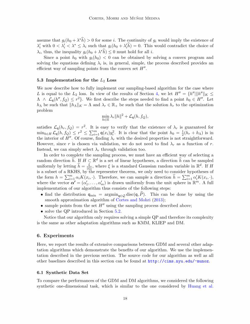
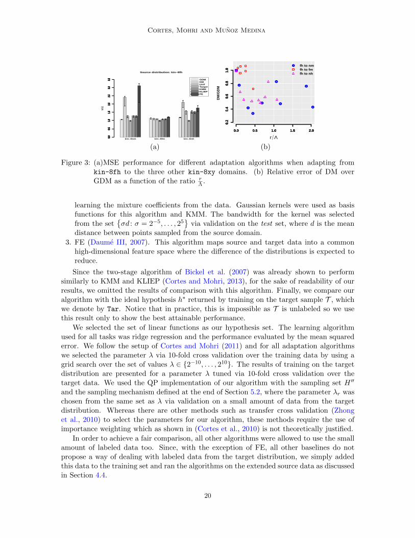
Figure 3: (a)MSE performance for different adaptation algorithms when adapting fromkin-8fh to the three other kin-8xy domains. (b) Relative error of DM overGDM as a function of the ratio r

Λ .

learning the mixture coefficients from the data. Gaussian kernels were used as basisfunctions for this algorithm and KMM. The bandwidth for the kernel was selectedfrom the set

{σd : σ = 2−5, . . . , 25

}via validation on the test set, where d is the mean

distance between points sampled from the source domain.

3. FE (Daume III, 2007). This algorithm maps source and target data into a commonhigh-dimensional feature space where the difference of the distributions is expected toreduce.

Since the two-stage algorithm of Bickel et al. (2007) was already shown to performsimilarly to KMM and KLIEP (Cortes and Mohri, 2013), for the sake of readability of ourresults, we omitted the results of comparison with this algorithm. Finally, we compare ouralgorithm with the ideal hypothesis h∗ returned by training on the target sample T , whichwe denote by Tar. Notice that in practice, this is impossible as T is unlabeled so we usethis result only to show the best attainable performance.

We selected the set of linear functions as our hypothesis set. The learning algorithmused for all tasks was ridge regression and the performance evaluated by the mean squarederror. We follow the setup of Cortes and Mohri (2011) and for all adaptation algorithmswe selected the parameter λ via 10-fold cross validation over the training data by using agrid search over the set of values λ ∈ {2−10, . . . , 210}. The results of training on the targetdistribution are presented for a parameter λ tuned via 10-fold cross validation over thetarget data. We used the QP implementation of our algorithm with the sampling set H ′′

and the sampling mechanism defined at the end of Section 5.2, where the parameter λr waschosen from the same set as λ via validation on a small amount of data from the targetdistribution. Whereas there are other methods such as transfer cross validation (Zhonget al., 2010) to select the parameters for our algorithm, these methods require the use ofimportance weighting which as shown in (Cortes et al., 2010) is not theoretically justified.

In order to achieve a fair comparison, all other algorithms were allowed to use the smallamount of labeled data too. Since, with the exception of FE, all other baselines do notpropose a way of dealing with labeled data from the target distribution, we simply addedthis data to the training set and ran the algorithms on the extended source data as discussedin Section 4.4.

20


Task: SentimentS T GDM DM Unif Tar KMM KLIEP F

B

K 0.763±(0.222) 1.056±(0.289) 1.00 0.517±(0.152) 3.328±(0.845) 3.494±(1.144) 0.942±(0.093)

E 0.574±(0.211) 1.018±(0.206) 1.00 0.367±(0.124) 3.018±(0.319) 3.022±(0.318) 0.857±(0.135)

D 0.936±(0.256) 1.215±(0.255) 1.00 0.623±(0.152) 2.842±(0.492) 2.764±(0.446) 0.936±(0.110)

K

B 0.854±(0.119) 1.258±(0.117) 1.00 0.665±(0.085) 2.784±(0.244) 2.642±(0.218) 1.047±(0.047)

E 0.975±(0.131) 1.460±(0.633) 1.00 0.653±(0.201) 2.408±(0.582) 2.157±(0.255) 0.969±(0.131)

D 0.884±(0.101) 1.174±(0.140) 1.00 0.665±(0.071) 2.771±(0.157) 2.620±(0.210) 1.111±(0.059)

E

B 0.723±(0.138) 1.016±(0.187) 1.00 0.551±(0.109) 3.433±(0.694) 3.290±(0.583) 1.035±(0.059)

K 1.030±(0.312) 1.277±(0.283) 1.00 0.636±(0.176) 2.173±(0.249) 2.223±(0.293) 0.955±(0.199)

D 0.731±(0.171) 1.005±(0.166) 1.00 0.518±(0.117) 3.363±(0.402) 3.231±(0.483) 0.974±(0.102)

D

B 0.992±(0.191) 1.026±(0.090) 1.00 0.740±(0.138) 2.571±(0.616) 2.475±(0.400) 0.986±(0.041)

K 0.870±(0.212) 1.062±(0.318) 1.00 0.557±(0.137) 2.755±(0.375) 2.741±(0.347) 0.940±(0.087)

E 0.674±(0.135) 0.994±(0.171) 1.00 0.478±(0.098) 2.939±(0.501) 2.878±(0.418) 0.907±(0.081)

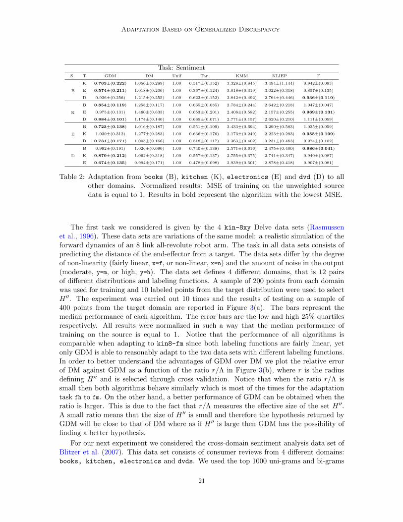
Table 2: Adaptation from books (B), kitchen (K), electronics (E) and dvd (D) to allother domains. Normalized results: MSE of training on the unweighted sourcedata is equal to 1. Results in bold represent the algorithm with the lowest MSE.

The first task we considered is given by the 4 kin-8xy Delve data sets (Rasmussenet al., 1996). These data sets are variations of the same model: a realistic simulation of theforward dynamics of an 8 link all-revolute robot arm. The task in all data sets consists ofpredicting the distance of the end-effector from a target. The data sets differ by the degreeof non-linearity (fairly linear, x=f, or non-linear, x=n) and the amount of noise in the output(moderate, y=m, or high, y=h). The data set defines 4 different domains, that is 12 pairsof different distributions and labeling functions. A sample of 200 points from each domainwas used for training and 10 labeled points from the target distribution were used to selectH ′′. The experiment was carried out 10 times and the results of testing on a sample of400 points from the target domain are reported in Figure 3(a). The bars represent themedian performance of each algorithm. The error bars are the low and high 25% quartilesrespectively. All results were normalized in such a way that the median performance oftraining on the source is equal to 1. Notice that the performance of all algorithms iscomparable when adapting to kin8-fm since both labeling functions are fairly linear, yetonly GDM is able to reasonably adapt to the two data sets with different labeling functions.In order to better understand the advantages of GDM over DM we plot the relative errorof DM against GDM as a function of the ratio r/Λ in Figure 3(b), where r is the radiusdefining H ′′ and is selected through cross validation. Notice that when the ratio r/Λ issmall then both algorithms behave similarly which is most of the times for the adaptationtask fh to fm. On the other hand, a better performance of GDM can be obtained when theratio is larger. This is due to the fact that r/Λ measures the effective size of the set H ′′.A small ratio means that the size of H ′′ is small and therefore the hypothesis returned byGDM will be close to that of DM where as if H ′′ is large then GDM has the possibility offinding a better hypothesis.

For our next experiment we considered the cross-domain sentiment analysis data set ofBlitzer et al. (2007). This data set consists of consumer reviews from 4 different domains:books, kitchen, electronics and dvds. We used the top 1000 uni-grams and bi-grams

21


Task: ImagesS T GDM DM Unif Tar KMM KLIEP F

C

I 0.927±(0.051) 1.005±(0.010) 1.00 0.879±(0.048) 2.752±(3.820) 0.936±(0.016) 0.959±(0.035)

S 0.938±(0.064) 0.993±(0.018) 1.00 0.840±(0.057) 0.827±(0.017) 0.835±(0.020) 0.947±(0.025)

B 0.909±(0.040) 1.003±(0.013) 1.00 0.886±(0.052) 0.945±(0.022) 0.942±(0.017) 0.947±(0.019)

I

C 1.011±(0.015) 0.951±(0.011) 1.00 0.802±(0.040) 0.989±(0.036) 1.009±(0.042) 0.971±(0.024)

S 1.006±(0.030) 0.992±(0.016) 1.00 0.871±(0.030) 0.930±(0.018) 0.936±(0.016) 0.973±(0.017)

B 0.987±(0.022) 1.009±(0.010) 1.00 0.986±(0.028) 1.011±(0.028) 1.011±(0.028) 0.994±(0.018)

S

C 1.022±(0.037) 0.982±(0.035) 1.00 0.759±(0.033) 1.172±(0.043) 1.201±(0.038) 0.938±(0.036)

I 0.924±(0.049) 0.998±(0.030) 1.00 0.831±(0.047) 3.868±(4.231) 1.227±(0.039) 0.947±(0.028)

B 0.898±(0.072) 1.003±(0.044) 1.00 0.821±(0.053) 1.240±(0.039) 1.248±(0.041) 0.945±(0.021)

B

C 1.010±(0.014) 0.956±(0.017) 1.00 0.777±(0.031) 1.028±(0.033) 1.032±(0.031) 0.980±(0.019)

I 1.012±(0.010) 1.004±(0.007) 1.00 0.966±(0.009) 2.785±(3.803) 0.981±(0.018) 1.000±(0.004)

S 1.009±(0.018) 0.988±(0.010) 1.00 0.850±(0.035) 0.930±(0.022) 0.934±(0.024) 0.983±(0.013)

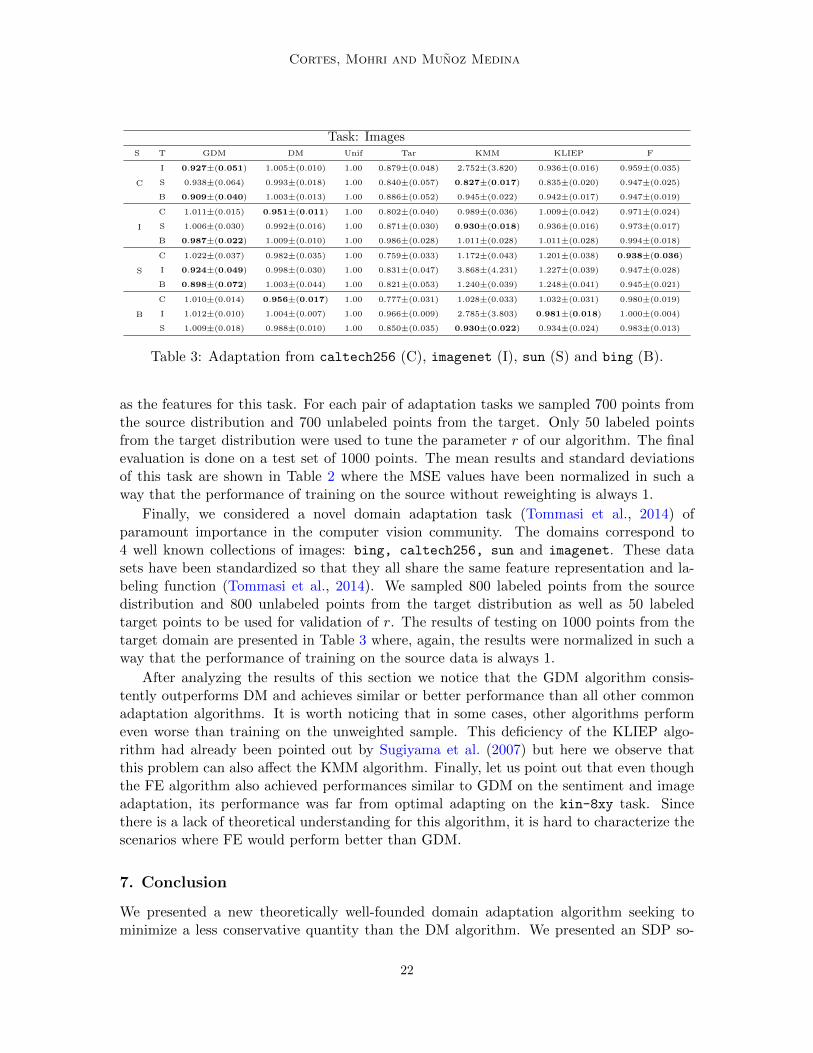
Table 3: Adaptation from caltech256 (C), imagenet (I), sun (S) and bing (B).

as the features for this task. For each pair of adaptation tasks we sampled 700 points fromthe source distribution and 700 unlabeled points from the target. Only 50 labeled pointsfrom the target distribution were used to tune the parameter r of our algorithm. The finalevaluation is done on a test set of 1000 points. The mean results and standard deviationsof this task are shown in Table 2 where the MSE values have been normalized in such away that the performance of training on the source without reweighting is always 1.

Finally, we considered a novel domain adaptation task (Tommasi et al., 2014) ofparamount importance in the computer vision community. The domains correspond to4 well known collections of images: bing, caltech256, sun and imagenet. These datasets have been standardized so that they all share the same feature representation and la-beling function (Tommasi et al., 2014). We sampled 800 labeled points from the sourcedistribution and 800 unlabeled points from the target distribution as well as 50 labeledtarget points to be used for validation of r. The results of testing on 1000 points from thetarget domain are presented in Table 3 where, again, the results were normalized in such away that the performance of training on the source data is always 1.

After analyzing the results of this section we notice that the GDM algorithm consis-tently outperforms DM and achieves similar or better performance than all other commonadaptation algorithms. It is worth noticing that in some cases, other algorithms performeven worse than training on the unweighted sample. This deficiency of the KLIEP algo-rithm had already been pointed out by Sugiyama et al. (2007) but here we observe thatthis problem can also affect the KMM algorithm. Finally, let us point out that even thoughthe FE algorithm also achieved performances similar to GDM on the sentiment and imageadaptation, its performance was far from optimal adapting on the kin-8xy task. Sincethere is a lack of theoretical understanding for this algorithm, it is hard to characterize thescenarios where FE would perform better than GDM.

7. Conclusion

We presented a new theoretically well-founded domain adaptation algorithm seeking tominimize a less conservative quantity than the DM algorithm. We presented an SDP so-

22


lution for the particular case of the L2 loss which can be solved in polynomial time. Ourempirical results show that our new algorithm always performs better than or is on parwith the otherwise state-of-the-art DM algorithm. We also provided tight generalizationbounds for the domain adaptation problem based on the Y-discrepancy. As pointed outin Section 4, an algorithm that minimizes the Y-discrepancy would benefit from the bestpossible guarantees. However, the lack of labeled data from the target distribution makesthis algorithm not viable. This suggests analyzing a richer scenario where the learner isallowed to ask for a limited number of labels from the target distribution. This setup, whichis related to active learning, seems to be in fact the closest one to real-life applications andhas started to receive attention from the research community (Berlind and Urner, 2015).We believe that the discrepancy disc will play a central role in the analysis of that scenarioas well.

Acknowledgments

We would like to thank the reviewers of KDD and JMLR for their suggestions to improvethis paper. This work was partly funded by the NSF awards IIS-1117591 and CCF-1535987.

Appendix A. SDP Formulation

Lemma 19 The Lagrangian dual of the problem

maxa∈Rm

‖Ksa−y‖2≤r2

1

2‖Ksta‖2 − b>KtKsta, (26)

is given by

minη≥0,γ

γ

s. t.

(−1

2K>stKst + ηK2s

12K>stKtb− ηKsy


)� 0.

Furthermore, the duality gap for these problems is zero.

Proof For η ≥ 0 the Lagrangian of (26) is given by

L(a, η) =1

2‖Ksta‖2 − b>KtKsta− η(‖Ksa− y‖2 − r2)

= a>(1

2K>stKst − ηK2

s

)a + (2ηKsy −K>stKtb)>a− η(‖y‖2 − r2).

Since the Lagrangian is a quadratic function of a and that the conjugate function of aquadratic can be expressed in terms of the pseudo-inverse, the dual is given by

minη≥0

1

4(2ηKsy −K>stKtb)>

(ηK2

s −1

2K>stKst

)†(2ηKsy −K>stKtb)− η(‖y‖2 − r2)

s. t. ηK2s −

1

2K>stKst � 0.

23


Introducing the variable γ to replace the objective function yields the equivalent problem

minη≥0,γ

γ

s. t. ηK2s −

1

2K>stKst � 0

γ − 1

4(2ηKsy −K>stKtb)>

(ηK2

s −1

2K>stKst

)†(2ηKsy −K>stKtb) + η(‖y‖2 − r2) ≥ 0

Finally, by the properties of the Schur complement (Boyd and Vandenberghe, 2004), thetwo constraints above are equivalent to

(−1

2K>stKst + ηK2s

12K>stKtb− ηKsy(

12K>stKtb− ηKsy

)>η(‖y‖2 − r) + γ

)� 0.

Since duality holds for a general QCQP with only one constraint (Boyd and Vandenberghe,2004)[Appendix B], the duality gap between these problems is 0.

Proposition 20 The optimization problem (23) is equivalent to the following SDP:

maxα,β,ν,Z,z

1


s. t

(νK2

s + 12K>stKst − 1

4K νKsy + 14Kz

νy>Ks + 14z>K α+ ν(‖y‖2 − r2)

)� 0 ∧

(Z zz> 1

)� 0

(λKt + K2

t12KtKstz

12z>K>stKt β

)� 0 ∧ Tr(K2

sZ)− 2y>Ksz + ‖y‖2 ≤ r2 ∧ ν ≥ 0,

where K = K>stKt(λKt + K2t )†KtKst.

ProofBy Lemma 16, we may rewrite (23) as

mina,γ,η,b

b>(λKt + K2t )b +

1

2a>K>stKsta− a>K>stKtb + γ (27)

s. t.

(−1

2K>stKst + ηK2s

12K>stKtb− ηKsy


)∧ η ≥ 0

‖Ksa− y‖2 ≤ r2.

Let us apply the change of variables b = 12(λKt+K2

t )†KtKsta+v. The following equalities

can be easily verified.

b>(λKt + K2t )b =

1

4a>K>stKt(λKt + K2

t )†KtKsta + v>KtKsta + v>(λKt + K2

t )v.

a>K>stKtb =1

2a>K>stKt(λKt + K2

t )†KtKsta + v>KtKsta.

24


Thus, replacing b on (27) yields

mina,v,γ,η

v>(λKt + K2t )v + a>

(1

2K>stKst −

1

4K)a + γ

s. t.

(−1

2K>stKst + ηK2s

14Ka + 1

2K>stKtv − ηKsy14a>K + 1

2v>KtKst − ηy>Ks η(‖y‖2 − r2) + γ

)� 0 ∧ η ≥ 0

‖Ksa− y‖2 ≤ r2.

Introducing the scalar multipliers µ, ν ≥ 0 and the matrix(

Z zz> z,

)� 0

as a multiplier for the matrix constraint, we can form the Lagrangian:

L := v>(λKt + K2t )v + a>

(1

2K>stKst −

1

4K)a + γ − µη + ν(‖Ksa− y‖2 − r2)

− Tr

((Z zz z

)( −12K>stKst + ηK2

s14Ka + 1

2K>stKtv − ηKsy14a>K + 1

2v>KtKst − ηy>Ks η(‖y‖2 − r2) + γ

)).

The KKT conditions ∂L∂η = ∂L

∂γ = 0 trivially imply z = 1 and Tr(K2sZ)− 2y>Ksz + ‖y‖2 −

r2 + µ = 0. These constraints on the dual variables guarantee that the primal variables ηand γ will vanish from the Lagrangian, thus yielding

L =1

2Tr(K>stKstZ) + ν(‖y‖2 − r2) + v>(λKt + K2

t )v> − z>K>stKtv

+ a>(νK2

s +1

2K>stKst −

1

4K)a−

(2νKsy +

1

2Kz)>

a.

This is a quadratic function on the primal variables a and v with minimizing solutions

a =1

2

(νK2

s +1

2K>stKst −

1

4K)†(

2νKsy +1

2Kz)

and v =1

2(λKt + K2

t )†KtKstz,

and optimal value equal to the objective of the Lagrangian dual:

1

2Tr(K>stKstZ) + ν(‖y‖2 − r2)− 1

4z>Kz

− 1

4

(2νKsy +

1

2Kz)>(

νK2s +

1

2K>stKst −

1

4K)†(

2νKsy +1

2Kz).

As in Lemma 16, we apply the properties of the Schur complement to show that the dualis given by

maxα,β,ν,Z,z

1


s. t

(νK2

s + 12K>stKst − 1

4K νKsy + 14Kz

νy>Ks + 14z>K α+ ν(‖y‖2 − r2)

)� 0 ∧

(Z zz> 1

)� 0

Tr(K2sZ)− 2y>Ksz + ‖y‖2 ≤ r2 ∧ β ≥ 1

4z>Kz ∧ ν ≥ 0.

25


Finally, recalling the definition of K and using the Schur complement one more time wearrive to the final SDP formulation

maxα,β,ν,Z,z

1


s. t

(νK2

s + 12K>stKst − 1

4K νKsy + 14Kz

νy>Ks + 14z>K α+ ν(‖y‖2 − r2)

)� 0 ∧

(Z zz> 1

)� 0

(λKt + K2

t12KtKstz

12z>K>stKt β

)� 0 ∧ Tr(K2

sZ)− 2y>Ksz + ‖y‖2 ≤ r2 ∧ ν ≥ 0.

Appendix B. QP Formulation

Proposition 21 Let Y = (Yij) ∈ Rn×k be the matrix defined by Yij = n−1/2hj(x′i) and

y′ = (y′1, . . . , y′k)> ∈ Rk the vector defined by y′i = n−1

∑nj=1 hi(x

′j)

2. Then, the dualproblem of (24) is given by

maxα,γ,β

−(Yα+

γ

2

)>Kt

(λI +

1

2Kt

)−1(Yα+

γ

2

)− 1

2γ>KtK

†tγ +α>y′ − β (28)

s.t. 1>α =1

2, 1β ≥ −Y>γ, α ≥ 0,

where 1 is the vector in Rk with all components equal to 1. Furthermore, the solution hof (24) can be recovered from a solution (α,γ, β) of (28) by ∀x, h(x) =

∑ni=1 aiK(xi, x),

where a =(λI + 1

2Kt)−1(Yα+ 1

2γ).

We will first prove a simplified version of the proposition for the case of linear hypotheses,i.e. we can represent hypotheses in H and elements of X as vectors w,x ∈ Rd respectively.Define X′ = n−1/2(x′1, . . . ,x

′n) to be the matrix whose columns are the normalized sample

points from the target distribution. Let also {w1, . . . ,wk} be a sample taken from ∂H ′′ anddefine W := (w1, . . . ,wk) ∈ Rd×k. Under this notation, problem (24) may be rewritten as

minw∈Rd

λ‖w‖2 +1

2maxi=1,...,k

‖X′>(w −wi)‖2 +1

2minw′∈C

‖X′>(w −w′)‖2. (29)

Lemma 22 The Lagrange dual of problem (29) is given by

maxα,γ,β

−(Yα+

γ

2

)>X′>

(λI+

X′X′>

2

)−1X′(Y α+

γ

2

)− 1

2γ>X′>(X′X′>)†X′γ +α>y′ − β

s. t. 1>α =1

21β ≥ −Y>γ α ≥ 0,

where Y = X′>W and y′i = ‖X′>wi‖2.

26


Proof By applying the change of variable u = w′ − w, problem (29) is can be madeequivalent to

minw∈Rdu∈C−w

λ‖w‖2 +1

2‖X′>w‖2 +

1

2‖X′>u‖2 +

1

2maxi=1,...,k

‖X′>wi‖2 − 2w>i X′X′>w.

By making the constraints on u explicit and replacing the maximization term with thevariable r the above problem becomes

minw,u,r,µ

λ‖w‖2 +1

2‖X′>w‖2 +

1

2‖X′>u‖2 +

1

2r

s. t. 1r ≥ y′ − 2Y>X′>w ∧ 1>µ = 1 ∧ µ ≥ 0 ∧ Wµ−w = u.

For α, δ ≥ 0, the Lagrangian of this problem is defined as

L(w,u,µ, r,α, β, δ,γ ′) = λ‖w‖2 +1

2‖X′>w‖2 +

1

2‖X′>u‖2 +

1

2r + β(1>µ− 1)

+α>(y′ − 2(X′Y)>w − 1r)− δ>µ+ γ ′>(Wµ−w − u).

Minimizing with respect to the primal variables yields the following KKT conditions:

1>α =1

21β = δ −W>γ ′. (30)

X′X′>u = γ ′ 2

(λI +

X′X′>

2

)w = 2(X′Y )α+ γ ′. (31)

Condition (30) implies that the terms involving r and µ will vanish from the Lagrangian.Furthermore, the first equation in (31) implies that any feasible γ ′ must satisfy γ ′ = X′γ for

some γ ∈ Rn. Finally, it is immediate that γ ′>u = u>X′X′>u and 2w>(λI + X′X′>

2

)w =

2α>(X′Y)>w + γ ′>w. Thus, at the optimal point, the Lagrangian becomes

−w>(λI +

1

2X′X′>

)w − 1

2u>X′X′>u +α>y′ − β

s. t. 1>α =1

21β = δ −W>γ ′ α ≥ 0 ∧ δ ≥ 0.

The positivity of δ implies that 1β ≥ −W>γ ′. Solving for w and u on (31) and applyingthe change of variable X′γ = γ ′ we obtain the final expression for the dual problem:

maxα,γ,β

−(Yα+

γ

2

)>X′>

(λI+

X′X′>

2

)−1X′(Y α+

γ

2

)− 1

2γ>X′>(X′X′>)†X′γ +α>y′ − β

s. t. 1>α =1

21β ≥ −Y>γ α ≥ 0,

where we have used the fact that Y>γ = WX′>γ to simplify the constraints. Notice alsothat we can recover the solution w of problem (29) as w = (λI + 1

2X′>X′)−1X′(Yα+ 12γ)

The proof of Proposition 18 follows from a straightforward application of the wellknown matrix identities X′(λI + X′>X′)−1 = (λI + X′X′>)−1X′ and X′>X′(X′>X′)† =X′>(X′X′>)†X′, and by the fact that the kernel matrix Kt is equal to X′>X′.

27


Appendix C. µ-admissibility

Lemma 23 Assume that Lp(h(x), y) ≤M for all x ∈ X and y ∈ Y, then Lp is µ-admissiblewith µ = pMp−1.

Proof Since x 7→ xp is p-Lipschitz over [0, 1] we can write

|L(h(x), y)− L(h′(x), y)| = Mp

∣∣∣∣( |h(x)− y|

M

)p−( |h′(x)− y|

M

)p∣∣∣∣≤ pMp−1|h(x)− y + y − h′(x)| = pMp−1|h(x)− h′(x)|,


Lemma 24 Let L be the Lp loss for some p ≥ 1 and let h, h′, h′′ be functions satisfyingLp(h(x), h′(x)) ≤ M and Lp(h

′′(x), h′(x)) ≤ M for all x ∈ X , for some M ≥ 0. Then, forany distribution D over X , the following inequality holds:

|LD(h, h′)− LD(h′′, h′)| ≤ pMp−1[LD(h, h′′)]1p . (32)

Proof Proceeding as in the proof of Lemma 23, we obtain

|LD(h, h′)− LD(h′′, h′)| = | Ex∈D

[Lp(h(x), h′(x))− Lp(h′′(x), h′(x)

]|

≤ pMp−1 Ex∈D

[|h(x)− h′′(x)|

].

Since p ≥ 1, by Jensen’s inequality, we can write Ex∈D[|h(x) − h′′(x)|

]≤ Ex∈D

[|h(x) −

h′′(x)|p]1/p

= [LD(h, h′′)]1p .

References

Shai Ben-David and Ruth Urner. On the hardness of domain adaptation and the utility ofunlabeled target samples. In Proceedings of ALT, pages 139–153, 2012.

Shai Ben-David, John Blitzer, Koby Crammer, and Fernando Pereira. Analysis of repre-sentations for domain adaptation. In Proceedings of NIPS, pages 137–144, 2006.

Shai Ben-David, Tyler Lu, Teresa Luu, and David Pal. Impossibility theorems for domainadaptation. JMLR - Proceedings Track, 9:129–136, 2010.

Christopher Berlind and Ruth Urner. Active nearest neighbors in changing environments.In Proceedings of ICML, pages 1870–1879, 2015.

Steffen Bickel, Michael Bruckner, and Tobias Scheffer. Discriminative learning for differingtraining and test distributions. In Proceedings of ICML, pages 81–88, 2007.

28


John Blitzer, Mark Dredze, and Fernando Pereira. Biographies, bollywood, boom-boxesand blenders: Domain adaptation for sentiment classification. In Proceedings of ACL,2007.

Stephen Boyd and Lieven Vandenberghe. Convex Optimization. Cambridge UniversityPress, Cambridge, 2004.

Corinna Cortes and Mehryar Mohri. Domain adaptation in regression. In Proceedings ofALT, 2011.

Corinna Cortes and Mehryar Mohri. Domain adaptation and sample bias correction theoryand algorithm for regression. Theoretical Computer Science, 9474, 2013.

Corinna Cortes, Mehryar Mohri, Michael Riley, and Afshin Rostamizadeh. Sample selectionbias correction theory. In Proceedings of ALT, pages 38–53, 2008.

Corinna Cortes, Yishay Mansour, and Mehryar Mohri. Learning bounds for importanceweighting. In Proceedings of NIPS, pages 442–450, 2010.

Hal Daume III. Frustratingly easy domain adaptation. In Proceedings of ACL, 2007.

Luc Devroye, Lazlo Gyorfi, and Gabor Lugosi. A Probabilistic Theory of Pattern Recogni-tion. Springer, 1996.

Mark Dredze, John Blitzer, Partha Pratim Talukdar, Kuzman Ganchev, Joao Graca, andFernando Pereira. Frustratingly hard domain adaptation for dependency parsing. InEMNLP-CoNLL, 2007.

Pascal Germain, Amaury Habrard, Francois Laviolette, and Emilie Morvant. A PAC-Bayesian approach for domain adaptation with specialization to linear classifiers. InProceedings of ICML, 2013.

Arthur Gretton, Karsten M. Borgwardt, Malte J. Rasch, Bernhard Scholkopf, and Alexan-der J. Smola. A kernel two-sample test. JMLR, 13:723–773, 2012.

Judy Hoffman, Trevor Darrell, and Kate Saenko. Continuous manifold based adaptationfor evolving visual domains. In Proceedings of IEEE CVPR, pages 867–874, 2014.

Jiayuan Huang, Alexander J. Smola, Arthur Gretton, Karsten M. Borgwardt, and BernhardScholkopf. Correcting sample selection bias by unlabeled data. In Proceedings of NIPS,volume 19, pages 601–608, 2006.

Jing Jiang and ChengXiang Zhai. Instance Weighting for Domain Adaptation in NLP. InProceedings of ACL, pages 264–271, 2007.

Piyush Kumar, Joseph S. B. Mitchell, and E. Alper Yildirim. Computing core-sets andapproximate smallest enclosing hyperspheres in high dimensions. In ALENEX, LectureNotes Comput. Sci, pages 45–55, 2003.

29


C. J. Leggetter and Philip C. Woodland. Maximum likelihood linear regression for speakeradaptation of continuous density hidden Markov models. Computer Speech & Language,9(2):171–185, 1995.

Yishay Mansour, Mehryar Mohri, and Afshin Rostamizadeh. Domain adaptation: Learningbounds and algorithms. In Proceedings of COLT. Omnipress, 2009.

Aleix M. Martınez. Recognizing imprecisely localized, partially occluded, and expressionvariant faces from a single sample per class. IEEE Trans. Pattern Anal., 24(6), 2002.

Andres Munoz Medina. Learning Theory and Algorithms for Auctioning and AdaptationProblems. PhD thesis, New York University, 2015.

Mehryar Mohri and Andres Munoz. New analysis and algorithm for learning with driftingdistributions. In Proceedings of ALT. Springer, 2012.

Sinno Jialin Pan, Ivor W. Tsang, James T. Kwok, and Qiang Yang. Domain adaptationvia transfer component analysis. IEEE Trans. on Neural Networks, 22(2):199–210, 2011.

Carl Edward Rasmussen, Radford M. Neal, Geoffrey Hinton, Drew van Camp, MichaelRevow Zoubin Ghahramani, Rafal Kustra, and Rob Tibshirani. The delve project. http://www.cs.toronto.edu/~delve/data/datasets.html, 1996. version 1.0.

Sven Schonherr. Quadratic Programming in Geometric Optimization: Theory, Implemen-tation, and Applications. PhD thesis, Swiss Federal Institute of Technology, 2002.

Masashi Sugiyama, Shinichi Nakajima, Hisashi Kashima, Paul von Bunau, and MotoakiKawanabe. Direct importance estimation with model selection and its application tocovariate shift adaptation. In Proceedings of NIPS, pages 1433–1440, 2007.

Tatiana Tommasi, Tinne Tuytelaars, and Barbara Caputo. A testbed for cross-datasetanalysis. CoRR, abs/1402.5923, 2014. URL http://arxiv.org/abs/1402.5923.

Leslie G. Valiant. A Theory of the Learnable. ACM Press New York, NY, USA, 1984.

Vladimir N. Vapnik. Statistical Learning Theory. J. Wiley & Sons, 1998.

E. Alper Yildirim. Two algorithms for the minimum enclosing ball problem. SIAM Journalon Optimization, 19(3):1368–1391, 2008.

Chao Zhang, Lei Zhang, and Jieping Ye. Generalization bounds for domain adaptation. InProceedings of NIPS, pages 1790–1798. MIT Press, 2012.

ErHeng Zhong, Wei Fan, Qiang Yang, Olivier Verscheure, and Jiangtao Ren. Cross valida-tion framework to choose amongst models and datasets for transfer learning. In Proceed-ings of ECML PKDD 2010 Part III, pages 547–562, 2010.

30

http://www.cs.toronto.edu/~delve/data/datasets.html

http://www.cs.toronto.edu/~delve/data/datasets.html

http://arxiv.org/abs/1402.5923

Documents

Adaptation Based on Generalized Discrepancy