Embed Size (px)
Citation preview
Adam PhillipsClimate Variability Working Group Liaison
CGD/NCAR
Thanks to Dennis Shea, Andrew Gettelman, and Christine Shields for their assistance
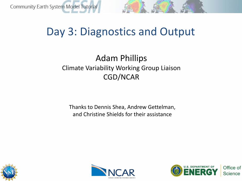
Day 3: Diagnostics and Output
OutlineI. CESM1.0 directory structures & file-naming conventionsII. Introduction to the netCDF format, ncdumpIII. netCDF Operators (NCO) / Climate Data Operators (CDO) / ncviewIV. Introduction to NCLV. ImageMagick / ghostviewVI. Practical Lab #3
A. Diagnostics packagesB. NCL post-processing scriptsC. NCL graphics scriptsD. Additional ExercisesE. Challenges
VII. Appendix (NCAR Archival System: The HPSS)
Day 3: Diagnostics and Output
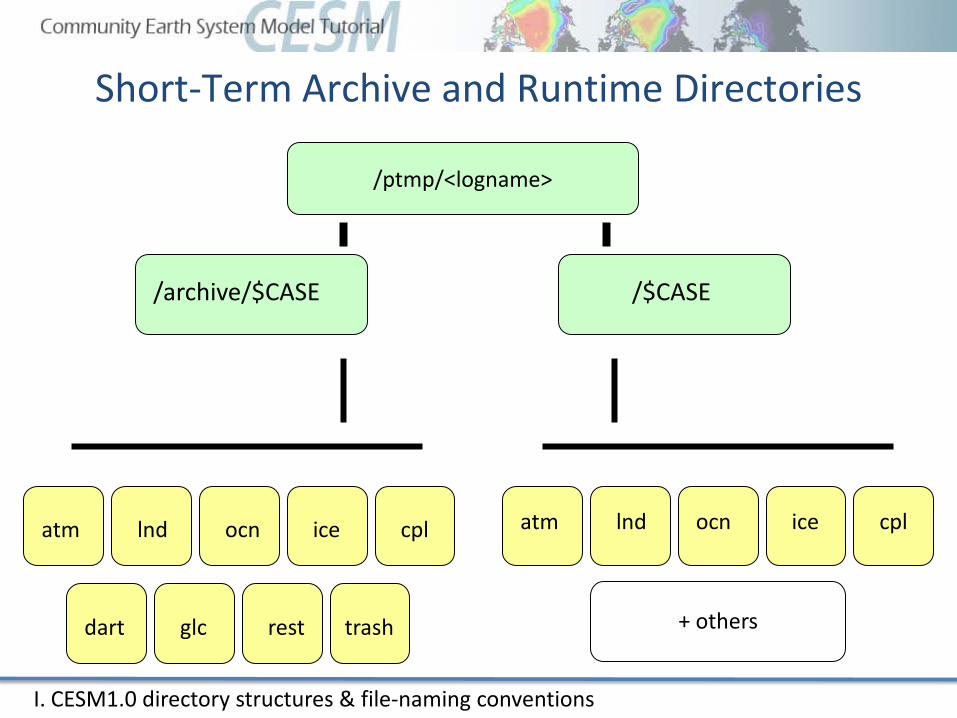
Short-Term Archive and Runtime Directories
/ptmp/<logname>
/$CASE/archive/$CASE
atm lnd ocn ice cpl
+ others
atm lnd ocn ice cpl
I. CESM1.0 directory structures & file-naming conventions
dart glc rest trash
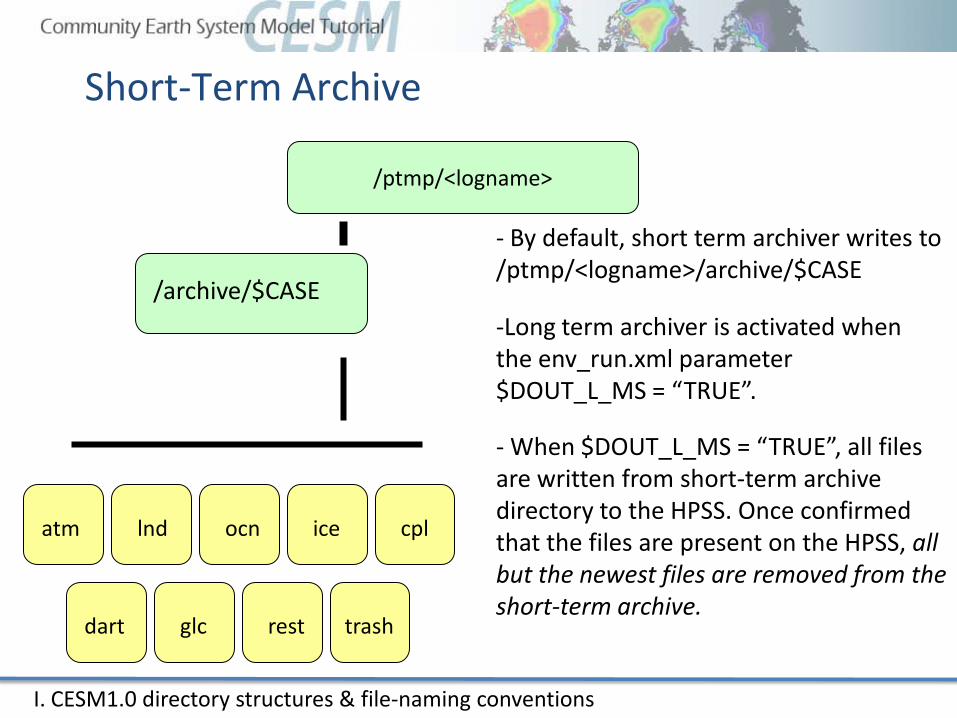
Short-Term Archive
/archive/$CASE
- By default, short term archiver writes to /ptmp/<logname>/archive/$CASE
- When $DOUT_L_MS = “TRUE”, all files are written from short-term archive directory to the HPSS. Once confirmed that the files are present on the HPSS, all but the newest files are removed from the short-term archive.
-Long term archiver is activated when the env_run.xml parameter $DOUT_L_MS = “TRUE”.
/ptmp/<logname>
I. CESM1.0 directory structures & file-naming conventions
atm lnd ocn ice cpl
dart glc rest trash
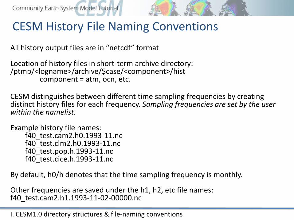
CESM History File Naming Conventions
Location of history files in short-term archive directory:/ptmp/<logname>/archive/$case/<component>/hist
component = atm, ocn, etc.
I. CESM1.0 directory structures & file-naming conventions
All history output files are in “netcdf” format
CESM distinguishes between different time sampling frequencies by creating distinct history files for each frequency. Sampling frequencies are set by the user within the namelist.
Example history file names:f40_test.cam2.h0.1993-11.ncf40_test.clm2.h0.1993-11.ncf40_test.pop.h.1993-11.ncf40_test.cice.h.1993-11.nc
By default, h0/h denotes that the time sampling frequency is monthly.
Other frequencies are saved under the h1, h2, etc file names: f40_test.cam2.h1.1993-11-02-00000.nc
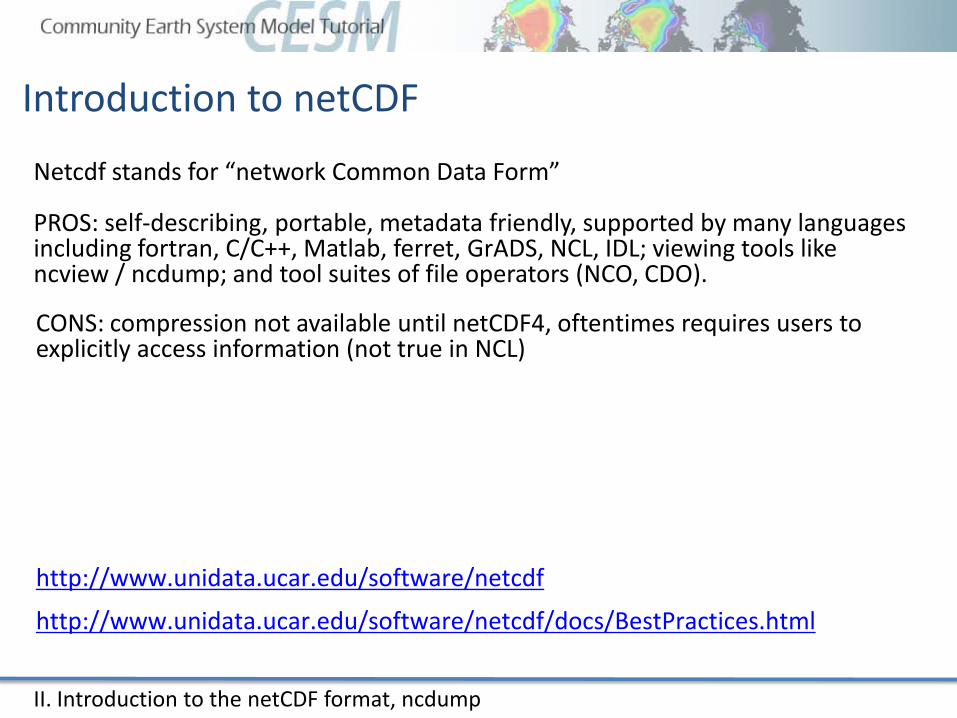
Introduction to netCDF
II. Introduction to the netCDF format, ncdump
Netcdf stands for “network Common Data Form”
PROS: self-describing, portable, metadata friendly, supported by many languages including fortran, C/C++, Matlab, ferret, GrADS, NCL, IDL; viewing tools like ncview / ncdump; and tool suites of file operators (NCO, CDO).
http://www.unidata.ucar.edu/software/netcdf
http://www.unidata.ucar.edu/software/netcdf/docs/BestPractices.html
CONS: compression not available until netCDF4, oftentimes requires users to explicitly access information (not true in NCL)
II. Introduction to the netCDF format, ncdump
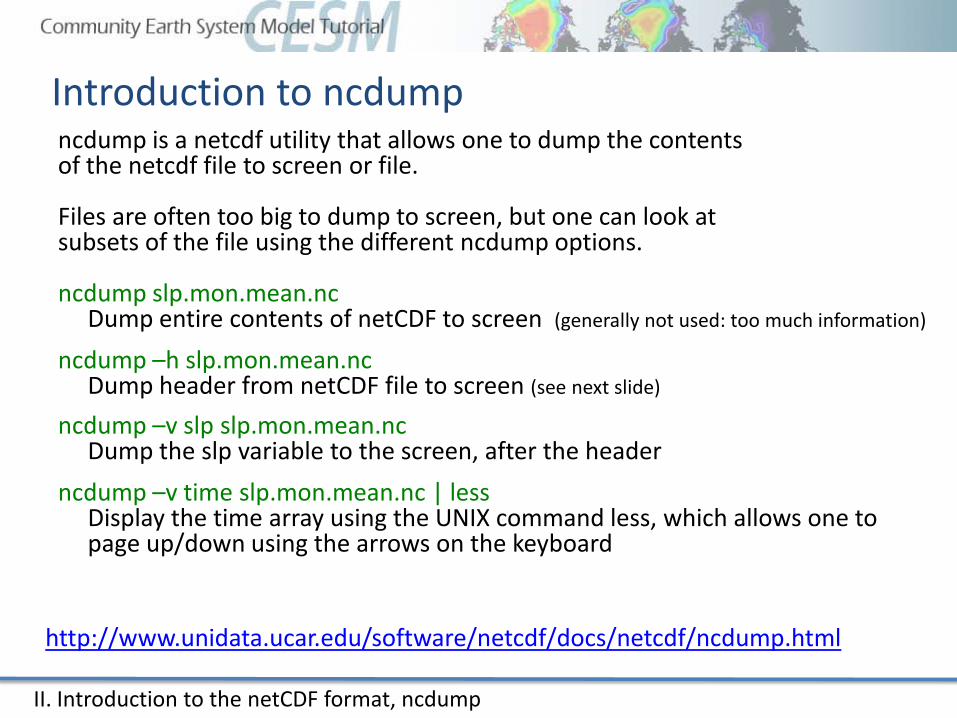
ncdump is a netcdf utility that allows one to dump the contents of the netcdf file to screen or file.
Files are often too big to dump to screen, but one can look at subsets of the file using the different ncdump options.
http://www.unidata.ucar.edu/software/netcdf/docs/netcdf/ncdump.html
ncdump slp.mon.mean.ncDump entire contents of netCDF to screen (generally not used: too much information)
Introduction to ncdump
ncdump –h slp.mon.mean.ncDump header from netCDF file to screen (see next slide)
ncdump –v slp slp.mon.mean.ncDump the slp variable to the screen, after the header
ncdump –v time slp.mon.mean.nc | lessDisplay the time array using the UNIX command less, which allows one to page up/down using the arrows on the keyboard
Example output using ncdump –h
II. Introduction to the netCDF format, ncdump
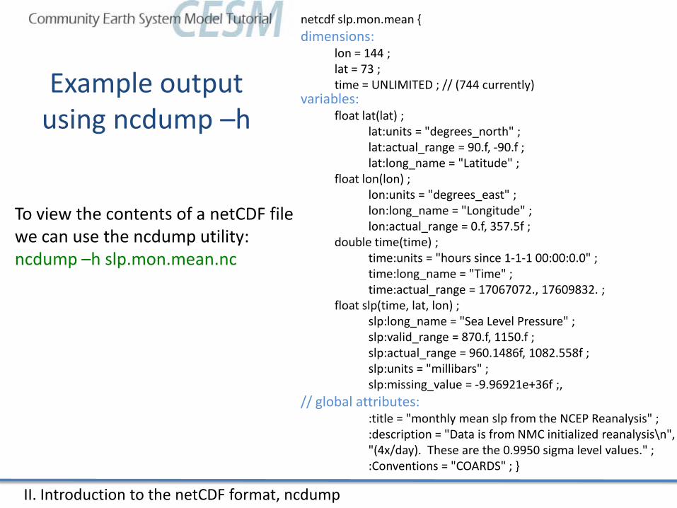
To view the contents of a netCDF file we can use the ncdump utility:ncdump –h slp.mon.mean.nc
netcdf slp.mon.mean dimensions:
lon = 144 ;lat = 73 ;time = UNLIMITED ; // (744 currently)
variables:float lat(lat) ;
lat:units = "degrees_north" ;lat:actual_range = 90.f, -90.f ;lat:long_name = "Latitude" ;
float lon(lon) ;lon:units = "degrees_east" ;lon:long_name = "Longitude" ;lon:actual_range = 0.f, 357.5f ;
double time(time) ;time:units = "hours since 1-1-1 00:00:0.0" ;time:long_name = "Time" ;time:actual_range = 17067072., 17609832. ;
float slp(time, lat, lon) ;slp:long_name = "Sea Level Pressure" ;slp:valid_range = 870.f, 1150.f ;slp:actual_range = 960.1486f, 1082.558f ;slp:units = "millibars" ;slp:missing_value = -9.96921e+36f ;,
// global attributes::title = "monthly mean slp from the NCEP Reanalysis" ;:description = "Data is from NMC initialized reanalysis\n","(4x/day). These are the 0.9950 sigma level values." ;:Conventions = "COARDS" ;
Introduction to netCDF operators (NCO)NCO is a suite of programs designed to perform certain “operations” on
netcdf files, i.e., things like averaging, concatenating, subsetting, or metadata manipulation.
Command-line operations are extremely useful for processing model data given that modellers often work in a UNIX-type environment. The NCO’s do much of the “heavy lifting” behind the scenes in the diagnostics packages.
The NCO Homepage can be found at http://nco.sourceforge.net
The Operator Reference Manual can be found at:http://nco.sourceforge.net/nco.html#Operator-Reference-Manual
Note: There are many other netCDF operators beyond what will be described here.
III. netCDF Operators (NCO) / Climate Data Operators (CDO) / ncview
UNIX wildcards are accepted for many of the operators.
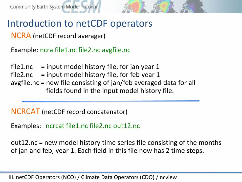
NCRA (netCDF record averager)
Example: ncra file1.nc file2.nc avgfile.nc
file1.nc = input model history file, for jan year 1file2.nc = input model history file, for feb year 1avgfile.nc = new file consisting of jan/feb averaged data for all
fields found in the input model history file.
NCRCAT (netCDF record concatenator)
Examples: ncrcat file1.nc file2.nc out12.nc
out12.nc = new model history time series file consisting of the months of jan and feb, year 1. Each field in this file now has 2 time steps.
Introduction to netCDF operators
III. netCDF Operators (NCO) / Climate Data Operators (CDO) / ncview
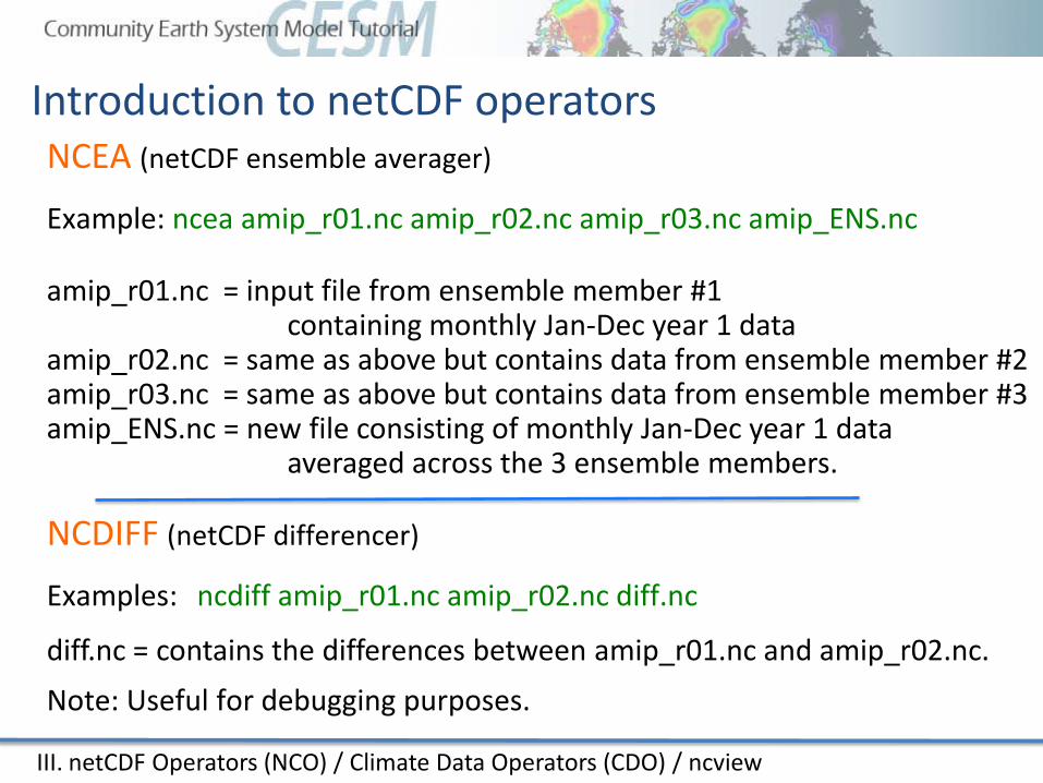
NCEA (netCDF ensemble averager)
Example: ncea amip_r01.nc amip_r02.nc amip_r03.nc amip_ENS.nc
amip_r01.nc = input file from ensemble member #1 containing monthly Jan-Dec year 1 data
amip_r02.nc = same as above but contains data from ensemble member #2amip_r03.nc = same as above but contains data from ensemble member #3 amip_ENS.nc = new file consisting of monthly Jan-Dec year 1 data
averaged across the 3 ensemble members.
NCDIFF (netCDF differencer)
Examples: ncdiff amip_r01.nc amip_r02.nc diff.nc
diff.nc = contains the differences between amip_r01.nc and amip_r02.nc.Note: Useful for debugging purposes.
Introduction to netCDF operators
III. netCDF Operators (NCO) / Climate Data Operators (CDO) / ncview
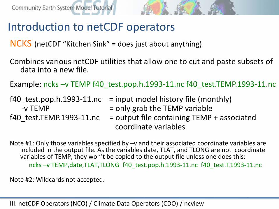
NCKS (netCDF “Kitchen Sink” = does just about anything)
Combines various netCDF utilities that allow one to cut and paste subsets of data into a new file.
Example: ncks –v TEMP f40_test.pop.h.1993-11.nc f40_test.TEMP.1993-11.nc
f40_test.pop.h.1993-11.nc = input model history file (monthly)-v TEMP = only grab the TEMP variable
f40_test.TEMP.1993-11.nc = output file containing TEMP + associated coordinate variables
Introduction to netCDF operators
Note #1: Only those variables specified by –v and their associated coordinate variables are included in the output file. As the variables date, TLAT, and TLONG are not coordinate variables of TEMP, they won’t be copied to the output file unless one does this:
ncks –v TEMP,date,TLAT,TLONG f40_test.pop.h.1993-11.nc f40_test.T.1993-11.nc
Note #2: Wildcards not accepted.
III. netCDF Operators (NCO) / Climate Data Operators (CDO) / ncview
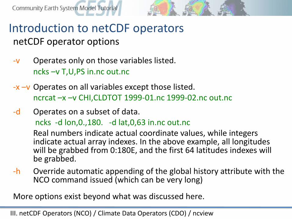
netCDF operator options
-v Operates only on those variables listed.ncks –v T,U,PS in.nc out.nc
-x –v Operates on all variables except those listed.ncrcat –x –v CHI,CLDTOT 1999-01.nc 1999-02.nc out.nc
More options exist beyond what was discussed here.
-h Override automatic appending of the global history attribute with the NCO command issued (which can be very long)
-d Operates on a subset of data.ncks -d lon,0.,180. -d lat,0,63 in.nc out.ncReal numbers indicate actual coordinate values, while integers indicate actual array indexes. In the above example, all longitudes will be grabbed from 0:180E, and the first 64 latitudes indexes will be grabbed.
Introduction to netCDF operators
III. netCDF Operators (NCO) / Climate Data Operators (CDO) / ncview
Introduction to Climate Data Operators (CDO)
III. netCDF Operators (NCO) / Climate Data Operators (CDO) / ncview
CDO are very similar to the NCO. They are similar simple command line operators that do a variety of tasks including: detrending, EOF analysis, and similar calculations.
The CDO Homepage can be found at:https://code.zmaw.de/projects/cdo/
CDO documentation can be found at:https://code.zmaw.de/projects/cdo/wiki/Cdo#Documentation
CDO are not currently used in the diagnostics packages, so we will not go into specifics here. We mention the CDO to make you aware of their existence.
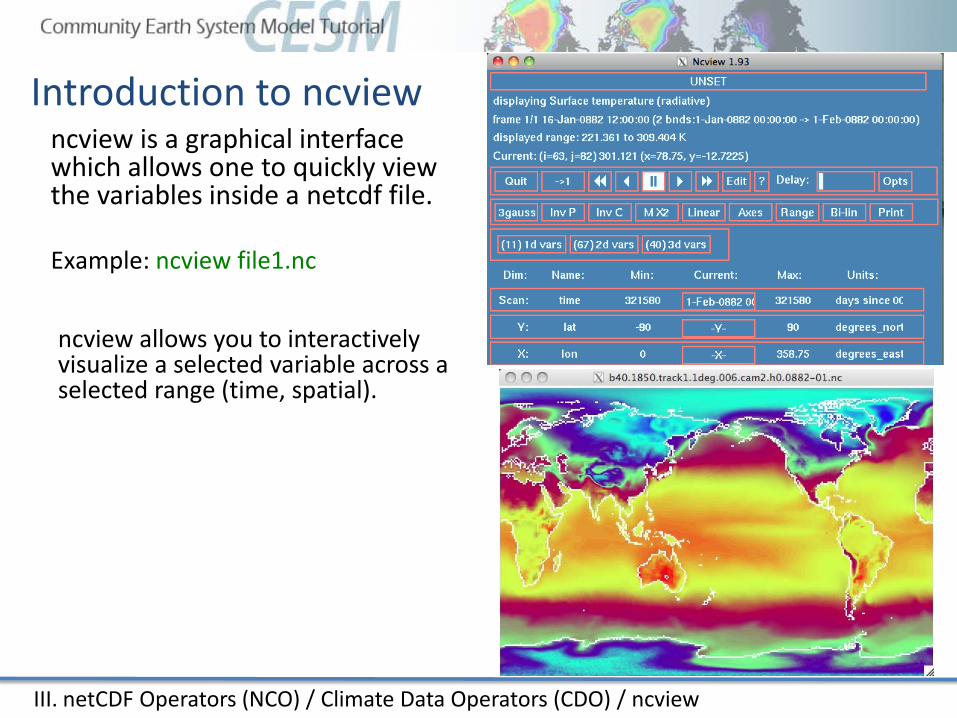
Introduction to ncviewncview is a graphical interface which allows one to quickly view the variables inside a netcdf file.
Example: ncview file1.nc
ncview allows you to interactively visualize a selected variable across a selected range (time, spatial).
III. netCDF Operators (NCO) / Climate Data Operators (CDO) / ncview
IV. Introduction to NCL
NCLNCL is an interpreted language designed for data processing and visualization. NCL is free, portable, allows for the creation of excellent graphics, can input/output multiple file formats, and contains numerous functions and procedures that make data processing easier. http://www.ncl.ucar.edu
NCL is the official CESM processing language.
Support: Postings to the ncl-talk email list are often answered within 24 hours by the NCL developers or by other NCL users.
Many downloadable examples are provided.
IV. Introduction to NCL
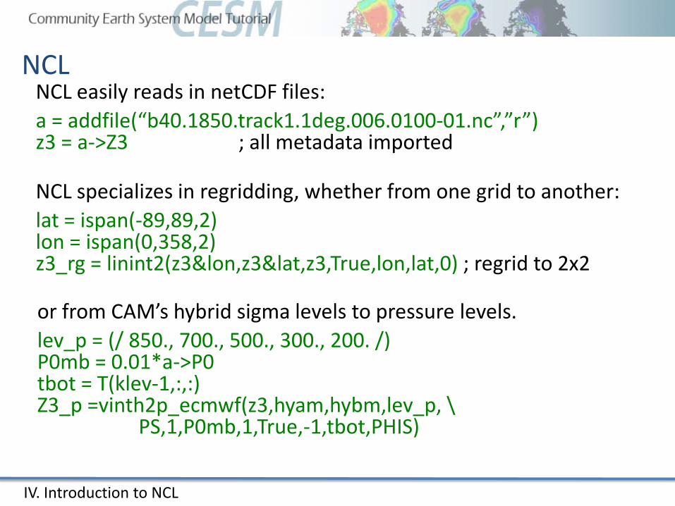
NCLNCL easily reads in netCDF files:a = addfile(“b40.1850.track1.1deg.006.0100-01.nc”,”r”)z3 = a->Z3 ; all metadata imported
NCL specializes in regridding, whether from one grid to another:lat = ispan(-89,89,2)lon = ispan(0,358,2)z3_rg = linint2(z3&lon,z3&lat,z3,True,lon,lat,0) ; regrid to 2x2
or from CAM’s hybrid sigma levels to pressure levels.lev_p = (/ 850., 700., 500., 300., 200. /) P0mb = 0.01*a->P0 tbot = T(klev-1,:,:) Z3_p =vinth2p_ecmwf(z3,hyam,hybm,lev_p, \
PS,1,P0mb,1,True,-1,tbot,PHIS)
IV. Introduction to NCL
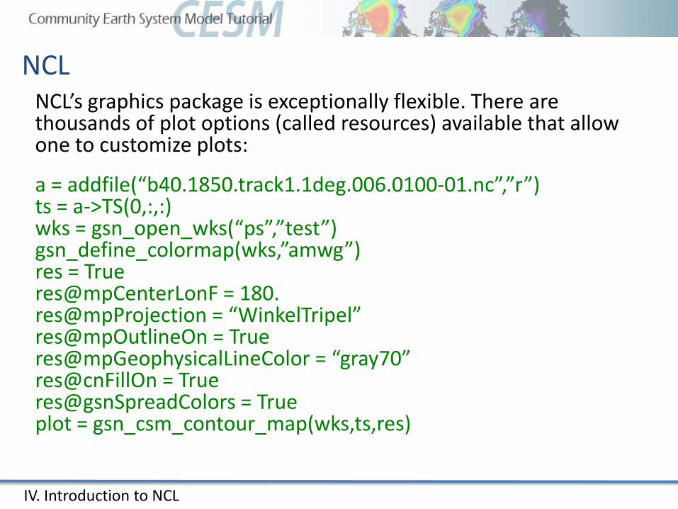
NCLNCL’s graphics package is exceptionally flexible. There are thousands of plot options (called resources) available that allow one to customize plots:
a = addfile(“b40.1850.track1.1deg.006.0100-01.nc”,”r”)ts = a->TS(0,:,:)wks = gsn_open_wks(“ps”,”test”)gsn_define_colormap(wks,”amwg”)res = Trueres@mpCenterLonF = 180.res@mpProjection = “WinkelTripel”res@mpOutlineOn = Trueres@mpGeophysicalLineColor = “gray70”res@cnFillOn = Trueres@gsnSpreadColors = Trueplot = gsn_csm_contour_map(wks,ts,res)
IV. Introduction to NCL
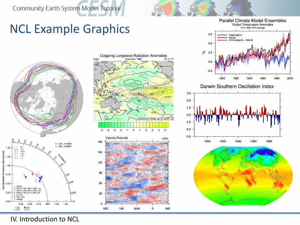
NCL Example Graphics
IV. Introduction to NCL
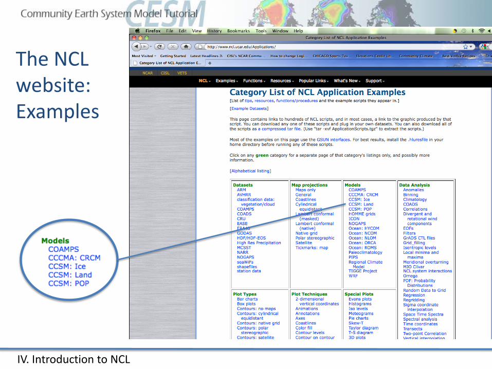
The NCL website: Examples
IV. Introduction to NCL
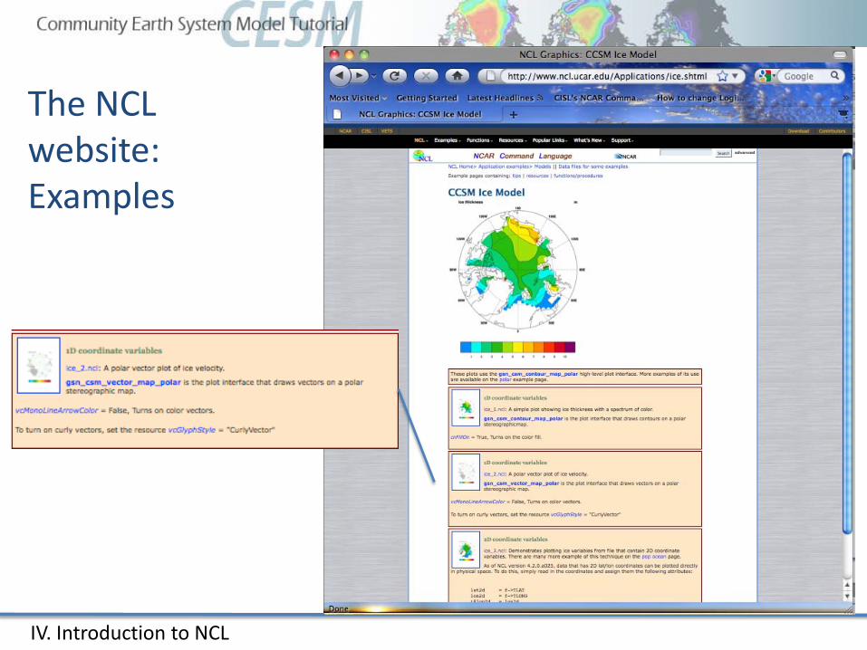
The NCL website: Examples
IV. Introduction to NCL
NCLFor more information, or to get started learning NCL:o http://www.ncl.ucar.edu/get_started.shtmlo Take the NCL class (information available on NCL website)o Page through the NCL mini-language and processing manuals
http://www.ncl.ucar.edu/Document/Manuals/
IV. Introduction to NCL
Using NCL in Practical Lab #3Within the lab, you are going to be provided NCL scripts that post-process the monthly model data that you created and draw simple graphics.
What is meant by post-processing: Convert the model history data from one time step all variables on one file to all time steps, one variable per file. (Also convert CAM 3D data from hybrid-sigma levels to selected pressure levels.)
The 4 diagnostic scripts (atmosphere, land, ice, ocean) all use NCL to varying degrees, and you will have the opportunity to run these as well.
V. ImageMagick / ghostview
ImageMagickImageMagick is a free suite of software that that can be used to display, manipulate, or convert images. It can also be used to create movies.
http://www.imagemagick.org
A second way is to alter an image at the command line, which is usually the faster and cleaner way to do it:convert –density 144 –rotate 270 -trim plot2.ps plot2.jpg
(set the resolution to 2x default, rotate the image 270 degrees, crop out all the possible white space, and convert to a jpg.)
There are two ways to use ImageMagick. One way is to simply display the image and alter it using pop-up menus:display plot1.png
To create a movie from the command line:convert –loop 0 –adjoin -delay 45 *.gif movie.gif
(loop through the movie once, create the movie (-adjoin),and increase the time between slides (-delay 0 is the default))
V. ImageMagick / ghostview
gv (Ghostview)gv and Gnome Ghostview are simple programs that allow one to view postscript files:
gv plot4.ps (gv) or ggv plot4.ps (gnome ghostview)(gv is installed on mirage cluster)
Once displayed, one can alter the orientation of the image, or change its’ size, or print specific pages amongst a group of pages. For viewing postscript (or encapsulated postscripts), gv should be used.
http://pages.cs.wisc.edu/~ghost/gv/index.htm
VI. Practical Lab #3
Practical Lab #3Within the lab, you will have the opportunity to play with the CESM history files that you created. There are 4 sets of diagnostics scripts, 4 NCL post-processing scripts, and 7 NCL graphics creating scripts. You will also be able to try out the various software packages discussed earlier (ncview, ImageMagick, etc.).
The following slides contain information about how to run the various scripts, along with exercises that you can try. It is suggested that you first focus on running those scripts written for the model component that you’re most interested in. For instance, if you’re an oceanographer, try running the ocean diagnostics script, along with the ocean post-processing script and ocean graphics NCL scripts.
Once you’ve completed running the scripts for your favorite component, take a run at the other model component scripts, or try the exercises or challenges on the last slide.
VI. Practical Lab #3
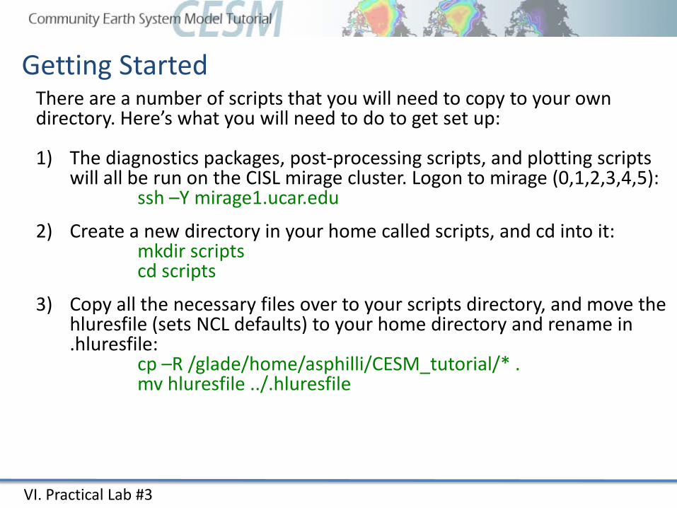
Getting StartedThere are a number of scripts that you will need to copy to your own directory. Here’s what you will need to do to get set up:
1) The diagnostics packages, post-processing scripts, and plotting scripts will all be run on the CISL mirage cluster. Logon to mirage (0,1,2,3,4,5):
ssh –Y mirage1.ucar.edu
2) Create a new directory in your home called scripts, and cd into it:mkdir scriptscd scripts
3) Copy all the necessary files over to your scripts directory, and move the hluresfile (sets NCL defaults) to your home directory and rename in .hluresfile:
cp –R /glade/home/asphilli/CESM_tutorial/* .mv hluresfile ../.hluresfile
VI. Practical Lab #3
Getting Started
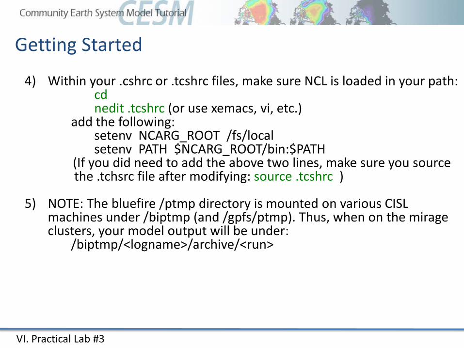
4) Within your .cshrc or .tcshrc files, make sure NCL is loaded in your path:cdnedit .tcshrc (or use xemacs, vi, etc.)
add the following: setenv NCARG_ROOT /fs/localsetenv PATH $NCARG_ROOT/bin:$PATH
(If you did need to add the above two lines, make sure you sourcethe .tchsrc file after modifying: source .tcshrc )
5) NOTE: The bluefire /ptmp directory is mounted on various CISL machines under /biptmp (and /gpfs/ptmp). Thus, when on the mirage clusters, your model output will be under:
/biptmp/<logname>/archive/<run>
VI. Practical Lab #3: Diagnostics Packages
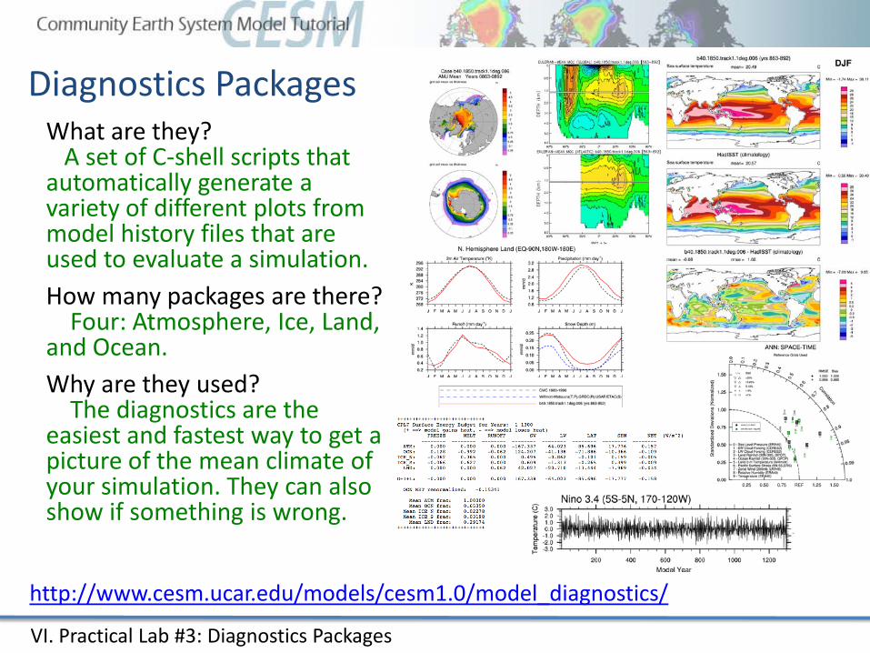
Diagnostics PackagesWhat are they?
A set of C-shell scripts that automatically generate a variety of different plots from model history files that are used to evaluate a simulation. How many packages are there?
Four: Atmosphere, Ice, Land, and Ocean.Why are they used?
The diagnostics are the easiest and fastest way to get a picture of the mean climate of your simulation. They can also show if something is wrong.
http://www.cesm.ucar.edu/models/cesm1.0/model_diagnostics/
VI. Practical Lab #3: Diagnostics Packages
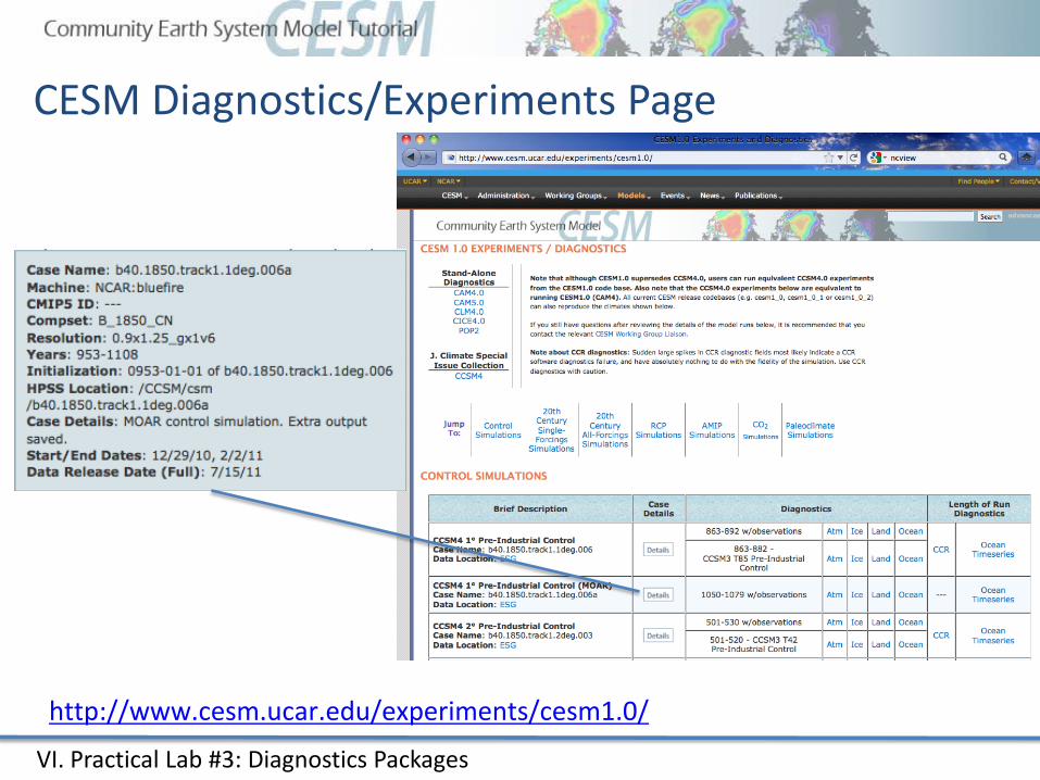
CESM Diagnostics/Experiments Page
http://www.cesm.ucar.edu/experiments/cesm1.0/
VI. Practical Lab #3: Diagnostics Packages
Diagnostics PackagesThe diagnostics packages were built to be flexible. Many comparisons are possible using the options provided.
Here, we have you set a few options to compare observations to your model run. You can also use the diagnostics to compare model runs to one another, regardless of model version.
The atmospheric, land, and ice packages each have one script that can do comparisons vs. observations or vs. another model run. The ocean diagnostics have three main scripts: popdiag (for comparison to observations), popdiagdiff (for comparison to another model run), and popdiagts (calculates various ocean time series).
Typically, 20 or 30 year time slices of data are analyzed using the diagnostics. (Exception: the popdiagts script is usually run on the entire run.) Here, you only have ~2 years of data, so that’s what we will use.
VI. Practical Lab #3: Diagnostics Packages
Diagnostics PackagesEach diagnostics package has different requirements in terms of the minimum amount of data required for them to run. (Ocean: 12 months, Atmosphere, Land: 14 months, Ice: 24 months) If you do not have the amount of data needed to run a specific diagnostics package, there is a directory set up with 3 years of CCSM4 pre-industrial control data for you to use here: /biptmp/asphilli/archive/b40.1850.track1.2deg.003
Note #1: Each diagnostics package will take around a 1/2hr to run. It is suggested that you start one of these packages first, and then move on to the post-processing or NCL graphics scripts.
Note #2: If you wish to take these diagnostics packages back with you to your home institution, you will need to have the netCDF operators and NCL installed (all 4 packages use it). For the ocean diagnostics package, you will also need ferret, IDL, and matlab.
VI. Practical Lab #3: Diagnostics Packages
AMWG Diagnostics PackageTo run the atmospheric diagnostics script (on mirage):
1) cd to your scripts directory, then into atm_diag:cd (changes to your home directory)cd scripts/atm_diag
2) Open up the file diag110520.csh using your favorite text editor:nedit diag110520.csh (or use xemacs, vi, etc.)
3) Modify the following lines and save the file:line 99 Enter your run namelines 101/102 Change “user” to your lognameline 114 Enter the model year you wish to start the diagnostics online 115 Enter the # of years you wish to analyze
4) Make the necessary atmospheric diagnostics directories:mkdir /ptmp/<logname>/amwgmkdir /ptmp/<logname>/amwg/climomkdir /ptmp/<logname>/amwg/diag
VI. Practical Lab #3: Diagnostics Packages
AMWG Diagnostics Package5) Submit the job, let it run in background mode, and write the output
to a file named atm.out:./diag110520.csh >&! atm.out &
6) If the diagnostics package errors out, check the output file atm.out, and correct the script.
7) Once the diagnostics script has successfully completed, a tar file should have been created here: /ptmp/<logname>/amwg/diag/<run>
8) cd to your diag directory, create a new directory called html, move the tar file to the html directory, and untar it:
cd /ptmp/<logname>/amwg/diag/<run>mkdir htmlmv *.tar html/cd htmltar –xf *.tar
VI. Practical Lab #3: Diagnostics Packages
AMWG Diagnostics Package8) cd into the new directory, fire up a firefox window, and open up the
index.html file:
cd <run>-obs/usr/bin/firefox &(File->Open File) then choose index.html
For reference: Your atmospheric diagnostics web files are located here:/ptmp/<logname>/atm_diag/html/<run>-obs/
For more information about the AMWG Diagnostics Package:http://www.cgd.ucar.edu/amp/amwg/diagnostics/index.html
VI. Practical Lab #3: Diagnostics Packages
LMWG Diagnostics PackageTo run the land model diagnostics script:1) cd to your scripts directory, then into lnd_diag:
cd (changes to your home directory)cd scripts/lnd_diag
2) Open up the file lnd_diag4.1.csh using your favorite text editor:nedit lnd_diag4.1.csh (or use xemacs, vi, etc.)
3) Modify the following lines:lines 66,67,68 Enter your run namelines 94,96 Change “user” to your lognameline 162 Enter the model year you wish to start the diagnostics online 163 Enter the # of years you wish to analyzeline 172 Set to same value as line 162 (can be different though)line 173 Set to same value as line 163 (again, can be different)
VI. Practical Lab #3: Diagnostics Packages
LMWG Diagnostics Package4) Submit the job, let it run in background mode, and write the output
to a file named lnd.out:./lnd_diag4.1.csh >&! lnd.out &
5) If the diagnostics package errors out, check the output file lnd.out, and correct the script.
6) Once the diagnostics script has successfully completed, a tar file should have been created in your ptmp directory: /ptmp/<logname>/<run>
7) cd to the new directory in /ptmp, create a new directory called html, move the tar file to the html directory, and untar it:
cd /ptmp/<logname>/<run>mkdir htmlmv *.tar html/cd htmltar –xf *.tar
VI. Practical Lab #3: Diagnostics Packages
LMWG Diagnostics Package8) cd into the new directory, fire up a firefox window, and open up the
setsIndex.html file:cd <run>-obs/usr/bin/firefox &(File->Open File) then choose setsIndex.html
For reference: Your land diagnostics web files are located here:/ptmp/<logname>/<run>/html/<run>-obs/
For more information about the LMWG Diagnostics Package:http://www.cgd.ucar.edu/tss/clm/diagnostics/webDir/lnd_diag4.1.htm
VI. Practical Lab #3: Diagnostics Packages
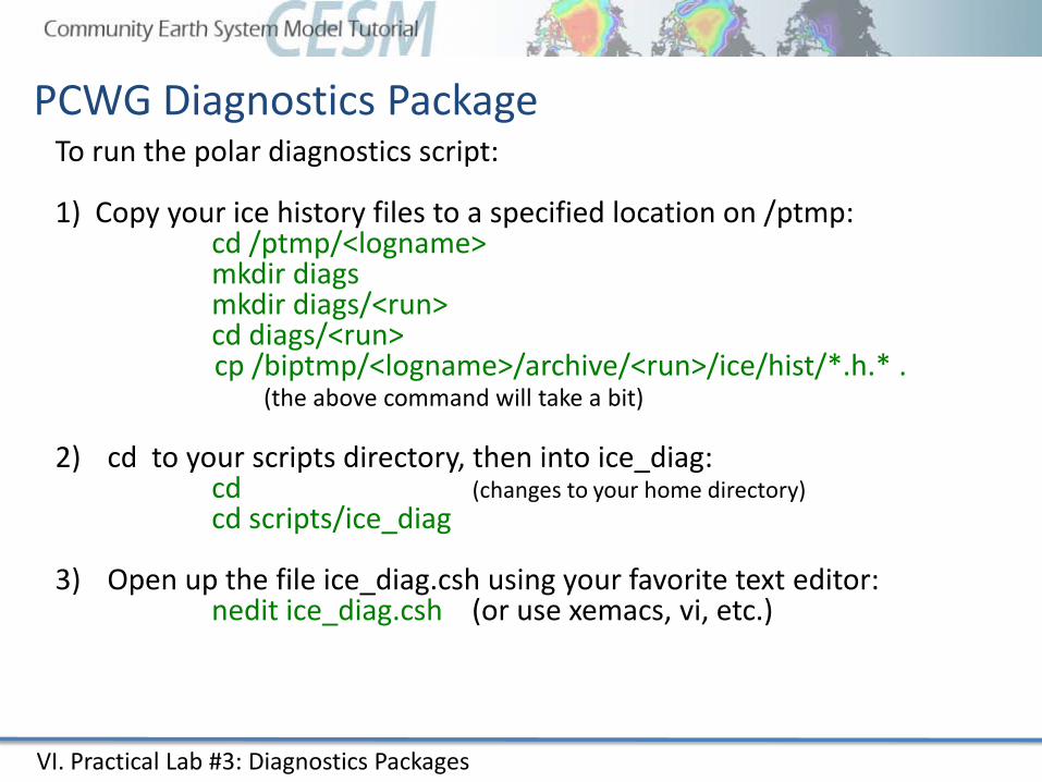
PCWG Diagnostics PackageTo run the polar diagnostics script:
1) Copy your ice history files to a specified location on /ptmp:cd /ptmp/<logname>mkdir diagsmkdir diags/<run>cd diags/<run>cp /biptmp/<logname>/archive/<run>/ice/hist/*.h.* .
(the above command will take a bit)
2) cd to your scripts directory, then into ice_diag:cd (changes to your home directory)cd scripts/ice_diag
3) Open up the file ice_diag.csh using your favorite text editor:nedit ice_diag.csh (or use xemacs, vi, etc.)
VI. Practical Lab #3: Diagnostics Packages
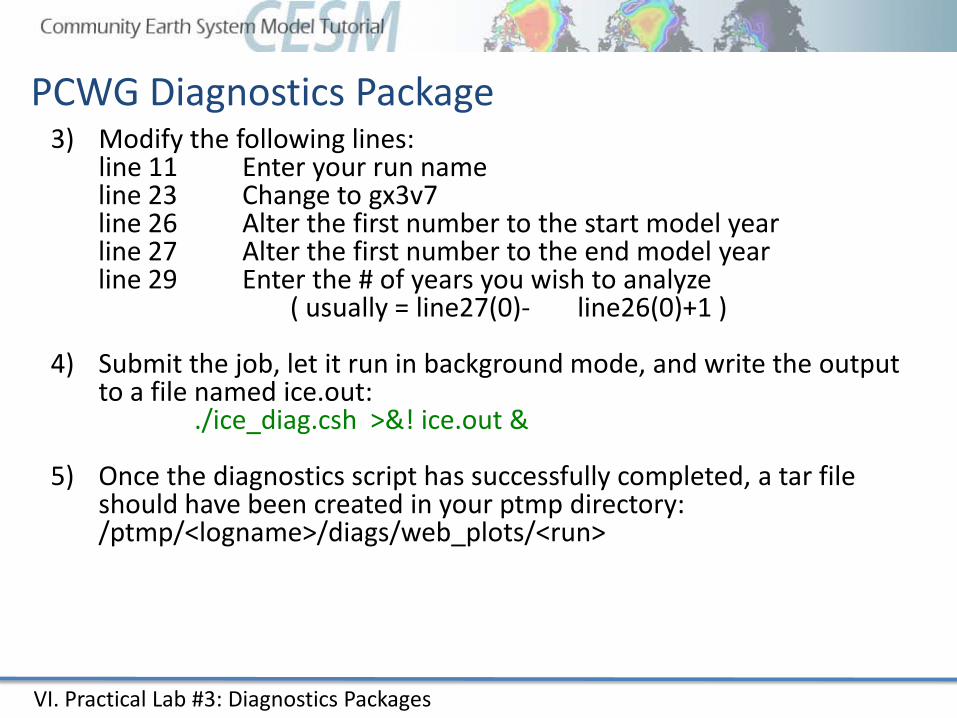
PCWG Diagnostics Package3) Modify the following lines:
line 11 Enter your run nameline 23 Change to gx3v7line 26 Alter the first number to the start model yearline 27 Alter the first number to the end model yearline 29 Enter the # of years you wish to analyze
( usually = line27(0)- line26(0)+1 )
4) Submit the job, let it run in background mode, and write the output to a file named ice.out:
./ice_diag.csh >&! ice.out &
5) Once the diagnostics script has successfully completed, a tar file should have been created in your ptmp directory: /ptmp/<logname>/diags/web_plots/<run>
VI. Practical Lab #3: Diagnostics Packages
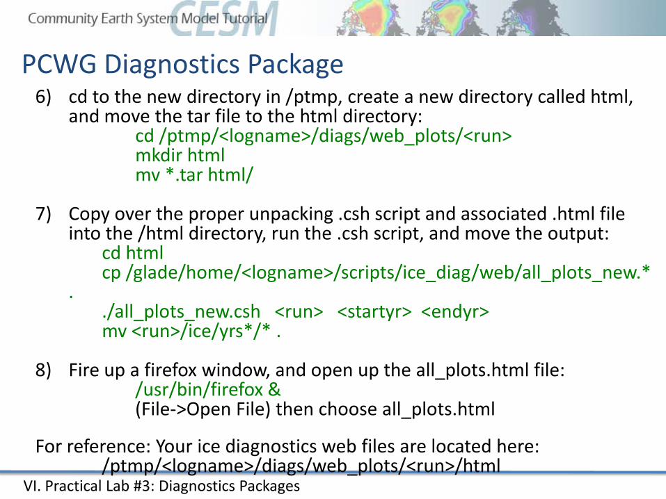
PCWG Diagnostics Package6) cd to the new directory in /ptmp, create a new directory called html,
and move the tar file to the html directory:cd /ptmp/<logname>/diags/web_plots/<run>mkdir htmlmv *.tar html/
7) Copy over the proper unpacking .csh script and associated .html file into the /html directory, run the .csh script, and move the output:
cd htmlcp /glade/home/<logname>/scripts/ice_diag/web/all_plots_new.*
../all_plots_new.csh <run> <startyr> <endyr>mv <run>/ice/yrs*/* .
8) Fire up a firefox window, and open up the all_plots.html file:/usr/bin/firefox &(File->Open File) then choose all_plots.html
For reference: Your ice diagnostics web files are located here:/ptmp/<logname>/diags/web_plots/<run>/html
VI. Practical Lab #3: Diagnostics Packages
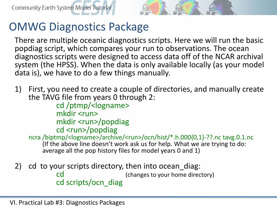
OMWG Diagnostics PackageThere are multiple oceanic diagnostics scripts. Here we will run the basic popdiag script, which compares your run to observations. The ocean diagnostics scripts were designed to access data off of the NCAR archival system (the HPSS). When the data is only available locally (as your model data is), we have to do a few things manually.
1) First, you need to create a couple of directories, and manually create the TAVG file from years 0 through 2:
cd /ptmp/<logname>mkdir <run>mkdir <run>/popdiagcd <run>/popdiag
ncra /biptmp/<logname>/archive/<run>/ocn/hist/*.h.0000,1-??.nc tavg.0.1.nc (If the above line doesn’t work ask us for help. What we are trying to do: average all the pop history files for model years 0 and 1)
2) cd to your scripts directory, then into ocean_diag:cd (changes to your home directory)cd scripts/ocn_diag

VI. Practical Lab #3: Diagnostics Packages
OMWG Diagnostics Package3) Open up the file popdiag.csh using your favorite text editor:
nedit popdiag.csh (or use xemacs, vi, etc.)
4) Modify the following lines:line 7 Enter your run nameline 8 Change to gx3v7line 9 Alter the first number to the start model yearline 10 Alter the first number to the end model yearline 61 replace CESM_tutorial with scripts
5) Submit the job, let it run in background mode, and write the output to a file named ice.out:
./popdiag.csh >&! ocn.out &
6) cd to the popdiag ptmp directory, start firefox, and look at popdiag.html:cd /ptmp/<logname>/<run>/popdiag/usr/bin/firefox &(File->Open File) then choose popdiag.html
VI. Practical Lab #3: Post-processing scripts
NCL post-processing scriptsAll 4 post-processing scripts are quite similar, and are located in your scripts directory. To list them, type: ls *create* . If these scripts are used for runs other than the tutorial runs, note that the created netCDF files may get quite large (especially pop files). This can be mitigated by setting concatand concat_rm = False.
To set up the post-processing scripts, alter lines 7-15 (7-17 for atm). There are comments to the right of each line explaining what each line does.
To run the atm script (for example), type the following:ncl atm.create_timeseries.ncl
All 4 scripts will write the post-processed data to work_dir (set at top of each script)/<run>. Once the post-processing is complete, we can use the new files in our NCL graphics scripts, or view them via ncview.
VI. Practical Lab #3: NCL graphics scripts
NCL Graphics ScriptsThese scripts are set up so that they can read either raw history files from your archive directory (lnd,ice,ocn history files) or the post-processed files after they’ve been created by the NCL post-processing scripts.
You will need to modify the user defined file inputs at the top to point to your data files, either your raw history files or your newly created post-processed files. Once the files are modified, to execute the scripts, simply type (for example):
ncl atm_latlon.ncl
There are 7 NCL graphics scripts available for you to run:atm_latlon.ncl atm_nino34_ts.ncl ice_south.nclice_north.ncl lnd_latlon.ncl ocn_latlon.nclocn_vectors.ncl
The ocn_vectors.ncl allows you to compare one ocean history file to another, and is more complicated (you can modify the first 50 lines) than the other 6 scripts. To run them, simply set the options at the top of the script.
VI. Practical Lab #3: Exercises
Exercises1) Use ncdump to examine one of the model history files. Find a variable
you’ve never heard of, then open up the same file using ncview, and plot that variable.
2) Modify one of the NCL scripts to plot a different variable.
3) Use the netCDF operators to difference two files. Plot various fields from the difference netCDF file using ncview.
4) Convert the output from one of the NCL scripts from .ps to .jpg, and crop out the white space. Import the image into Powerpoint.
5) Use the netCDF operators to concatenate sea level pressure and the variable date from all the monthly atmospheric history files (.h0.) into one file.
6) Same as 5), but only do this for the Northern Hemisphere.
7) Same as 6), but don’t append the global history file attribute.
VI. Practical Lab #3: Challenges
Challenges1) Modify one of the NCL scripts to alter the look of the plot. Use the
NCL website’s Examples page to assist.
2) Add a variable or 3 to one of the post-processing scripts, then modify one of the NCL scripts to plot one of the new variables.
3) Use the atmospheric diagnostics package to compare your simulation against the simulation here: /biptmp/asphilli/archive/b40.1850.track1.2deg.003 Make sure you compare the same number of years.
Introduction to the NCAR Archival SystemThe High Performance Storage System (HPSS)
• Tape-based archival system (same back end as MSS)• FTP-like interface• Connected to most CISL/CGD systems• Reading and writing methods [*]nix-like: cp, mv, put, get,…• Files do not expire, and can be as large as 1TB• By default, 1 tape copy of each file is created.
VII. Appendix
http://www2.cisl.ucar.edu/docs/hpss-guide
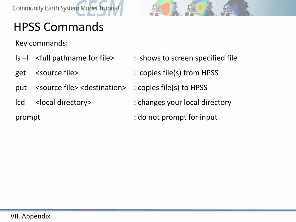
HPSS CommandsKey commands:
ls –l <full pathname for file> : shows to screen specified file
get <source file> : copies file(s) from HPSS
put <source file> <destination> : copies file(s) to HPSS
lcd <local directory> : changes your local directory
prompt : do not prompt for input
VII. Appendix
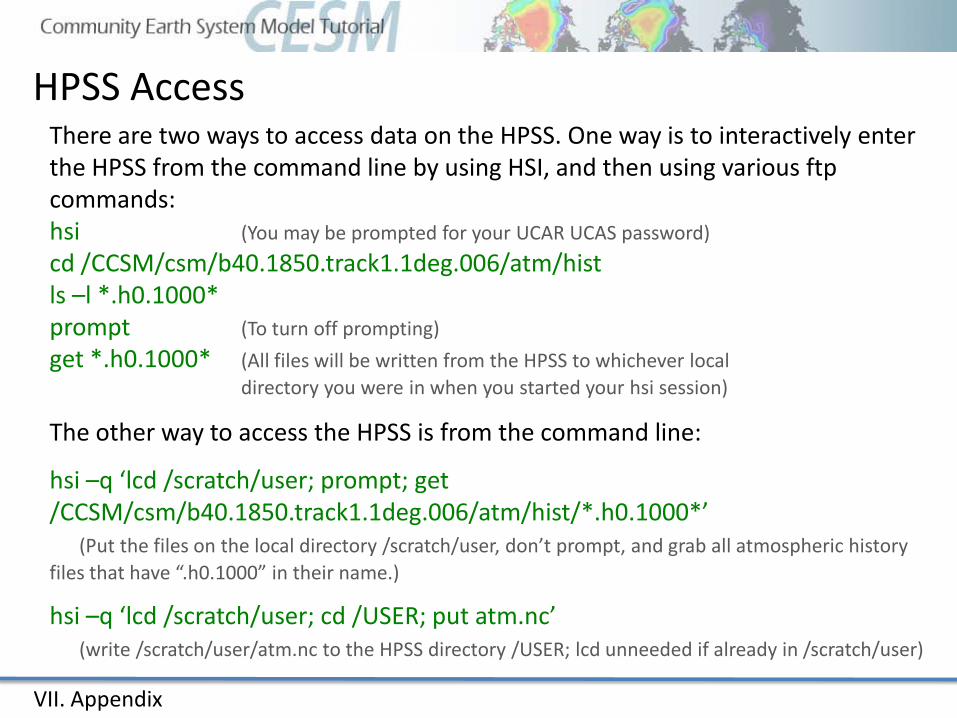
HPSS AccessThere are two ways to access data on the HPSS. One way is to interactively enter the HPSS from the command line by using HSI, and then using various ftp commands:hsi (You may be prompted for your UCAR UCAS password)cd /CCSM/csm/b40.1850.track1.1deg.006/atm/histls –l *.h0.1000*prompt (To turn off prompting)get *.h0.1000* (All files will be written from the HPSS to whichever local
directory you were in when you started your hsi session)
The other way to access the HPSS is from the command line:
hsi –q ‘lcd /scratch/user; prompt; get /CCSM/csm/b40.1850.track1.1deg.006/atm/hist/*.h0.1000*’
(Put the files on the local directory /scratch/user, don’t prompt, and grab all atmospheric history files that have “.h0.1000” in their name.)
hsi –q ‘lcd /scratch/user; cd /USER; put atm.nc’ (write /scratch/user/atm.nc to the HPSS directory /USER; lcd unneeded if already in /scratch/user)
VII. Appendix