ADAPTIVE RESONANT MODE ACTIVE NOISE

CONTROL

by

Adam K. Smith

BS, University of Pittsburgh, 2003

Submitted to the Graduate Faculty of

the School of Engineering in partial fulfillment

of the requirements for the degree of

Master of Science

University of Pittsburgh

2005

UNIVERSITY OF PITTSBURGH

SCHOOL OF ENGINEERING

This thesis was presented

by

Adam K. Smith

It was defended on

October 12, 2005

and approved by

Jeffrey S. Vipperman, Associate Professor, Mechanical Engineering Department

Daniel D. Budny, Associate Professor, Civil and Environmental Engineering Department

William W. Clark, Professor, Mechanical Engineering Department

Thesis Advisor: Jeffrey S. Vipperman, Associate Professor, Mechanical Engineering

Department

ii

ABSTRACT

ADAPTIVE RESONANT MODE ACTIVE NOISE CONTROL

Adam K. Smith, MS

University of Pittsburgh, 2005

Low frequency sound waves propagating in a duct is ideally suited for active noise control

(ANC) applications. Unlike passive treatments, ANC utilizes an acoustic actuator (loud-

speaker) to cancel unwanted sound fields. There are two main control topologies when

considering the active suppression of sound, feedforward and feedback. The former requires

that the disturbance be known before the control signal is generated, and is ideal for periodic

or random signals. Feedback arrangements, on the other hand, modify the dynamics of an

enclosured sound field to augment damping, and requires no a priori knowledge of the dis-

turbance. A modified version of feedback that is used in structures called positive position

feedback (PPF), can be applied to acoustic systems. In a previous study, a tuned resonant

filter modelled after a Helmholtz resonator was used in PPF configuration to suppress noise

levels by Bisnette and Vipperman (2004). However, the presence of speaker dynamics neces-

sitates further phase compensation, which is accomplished with an all-pass filter. The work

presented here further develops this control method by using a higher-order compensator. In

this study, band-pass filters are used to improve the multi-modal control by limiting phase

interaction of adjacent modes. Further refinements are made by realizing the control system

electronically, which gives the ability to adapt controller parameters. Here, an algorithm

is presented that adapts the resonant controller gain. Experimental results show moderate

reductions with no energy spill-over to the next adjacent uncontrolled mode.

iii

TABLE OF CONTENTS

1.0 INTRODUCTION . . . . . . . . . . . . . . . . . . . . . . . . . . . . . . . . . 1

2.0 THEORETICAL DEVELOPMENT . . . . . . . . . . . . . . . . . . . . . . 7

2.1 ANALYTICAL DUCT MODEL . . . . . . . . . . . . . . . . . . . . . . . . 7

2.1.1 Acoustic Enclosure . . . . . . . . . . . . . . . . . . . . . . . . . . . . 8

2.1.2 Acoustic Actuator . . . . . . . . . . . . . . . . . . . . . . . . . . . . . 9

2.2 UNCONTROLLED SYSTEM . . . . . . . . . . . . . . . . . . . . . . . . . . 10

3.0 CONTROL SIMULATION . . . . . . . . . . . . . . . . . . . . . . . . . . . 12

3.1 CONTROL SYSTEM CONFIGURATION . . . . . . . . . . . . . . . . . . . 13

3.2 COMPENSATOR DESIGN . . . . . . . . . . . . . . . . . . . . . . . . . . . 14

3.2.1 Resonant Compensating Filter . . . . . . . . . . . . . . . . . . . . . . 16

3.2.2 Phase Compensation . . . . . . . . . . . . . . . . . . . . . . . . . . . 20

3.3 SINGLE MODE CONTROL . . . . . . . . . . . . . . . . . . . . . . . . . . 21

3.4 MULTIPLE MODE CONTROL . . . . . . . . . . . . . . . . . . . . . . . . 25

4.0 EXPERIMENTAL DEMONSTRATION . . . . . . . . . . . . . . . . . . . 29

4.1 SINGLE MODE CONTROL . . . . . . . . . . . . . . . . . . . . . . . . . . 31

4.1.1 Collocated Control . . . . . . . . . . . . . . . . . . . . . . . . . . . . 32

4.1.2 Non-Collocated Control . . . . . . . . . . . . . . . . . . . . . . . . . . 35

4.2 MULTIPLE MODE CONTROL . . . . . . . . . . . . . . . . . . . . . . . . 38

5.0 ADAPTIVE CONTROL . . . . . . . . . . . . . . . . . . . . . . . . . . . . . 43

5.1 PRELIMINARY ADAPTIVE ALGORITHM . . . . . . . . . . . . . . . . . 44

5.2 ADAPTIVE CONTROL SIMULATION . . . . . . . . . . . . . . . . . . . . 48

5.3 EXPERIMENTAL ADAPTIVE CONTROL DEMONSTRATION . . . . . . 49

iv

6.0 CONCLUSIONS AND FUTURE WORK . . . . . . . . . . . . . . . . . . 52

APPENDIX A. MATLAB SIMULINKTM CODE FOR ADAPTIVE CON-

TROL SIMULATIONS . . . . . . . . . . . . . . . . . . . . . . . . . . . . . . 55

APPENDIX B. MATLAB SIMULINKTM CODE FOR ADAPTIVE CON-

TROL EXPERIMENTAL DEMONSTRATION . . . . . . . . . . . . . . 58

BIBLIOGRAPHY . . . . . . . . . . . . . . . . . . . . . . . . . . . . . . . . . . . . 60

v

LIST OF TABLES

1 Plant parameters used in simulation. . . . . . . . . . . . . . . . . . . . . . . . 11

2 Source loading measurements. . . . . . . . . . . . . . . . . . . . . . . . . . . 32

3 First 4 pressure nodes of the acoustic duct. . . . . . . . . . . . . . . . . . . . 38

vi

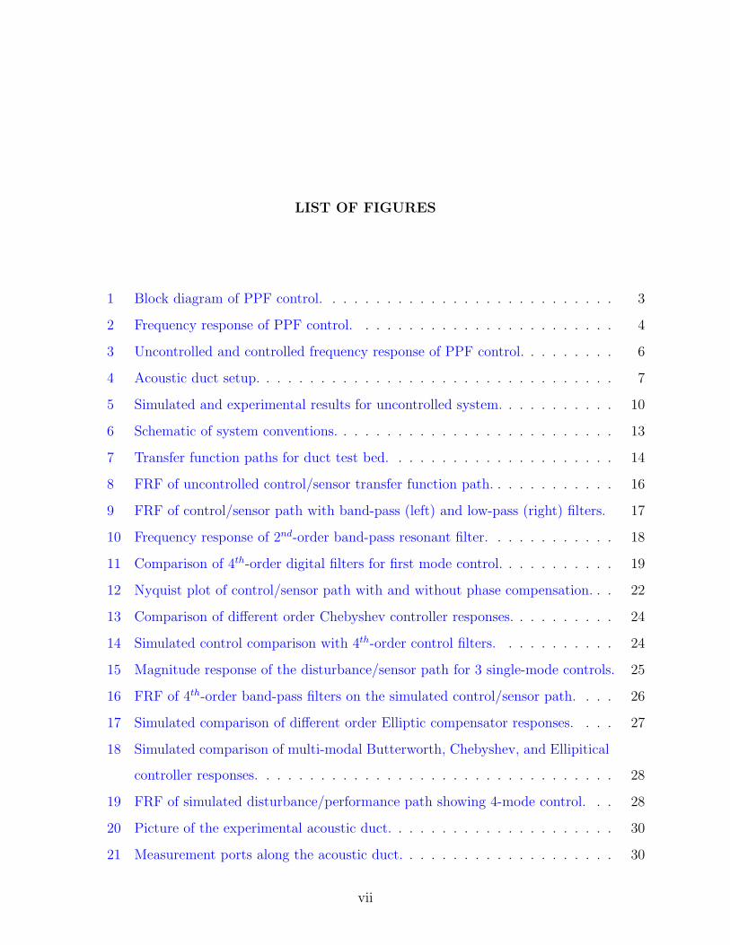
LIST OF FIGURES

1 Block diagram of PPF control. . . . . . . . . . . . . . . . . . . . . . . . . . . 3

2 Frequency response of PPF control. . . . . . . . . . . . . . . . . . . . . . . . 4

3 Uncontrolled and controlled frequency response of PPF control. . . . . . . . . 6

4 Acoustic duct setup. . . . . . . . . . . . . . . . . . . . . . . . . . . . . . . . . 7

5 Simulated and experimental results for uncontrolled system. . . . . . . . . . . 10

6 Schematic of system conventions. . . . . . . . . . . . . . . . . . . . . . . . . . 13

7 Transfer function paths for duct test bed. . . . . . . . . . . . . . . . . . . . . 14

8 FRF of uncontrolled control/sensor transfer function path. . . . . . . . . . . . 16

9 FRF of control/sensor path with band-pass (left) and low-pass (right) filters. 17

10 Frequency response of 2nd-order band-pass resonant filter. . . . . . . . . . . . 18

11 Comparison of 4th-order digital filters for first mode control. . . . . . . . . . . 19

12 Nyquist plot of control/sensor path with and without phase compensation. . . 22

13 Comparison of different order Chebyshev controller responses. . . . . . . . . . 24

14 Simulated control comparison with 4th-order control filters. . . . . . . . . . . 24

15 Magnitude response of the disturbance/sensor path for 3 single-mode controls. 25

16 FRF of 4th-order band-pass filters on the simulated control/sensor path. . . . 26

17 Simulated comparison of different order Elliptic compensator responses. . . . 27

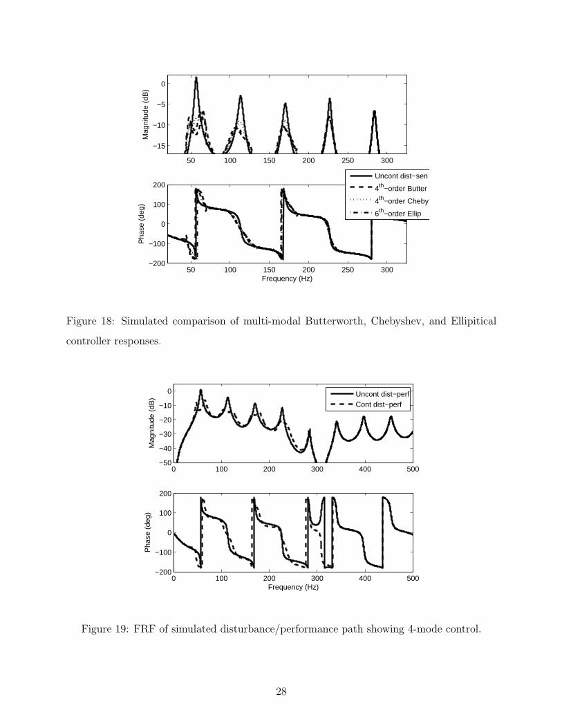
18 Simulated comparison of multi-modal Butterworth, Chebyshev, and Ellipitical

controller responses. . . . . . . . . . . . . . . . . . . . . . . . . . . . . . . . . 28

19 FRF of simulated disturbance/performance path showing 4-mode control. . . 28

20 Picture of the experimental acoustic duct. . . . . . . . . . . . . . . . . . . . . 30

21 Measurement ports along the acoustic duct. . . . . . . . . . . . . . . . . . . . 30

vii

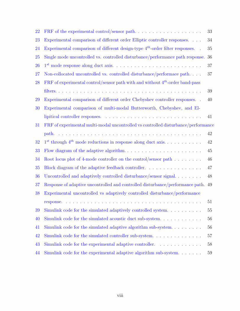
22 FRF of the experimental control/sensor path. . . . . . . . . . . . . . . . . . . 33

23 Experimental comparison of different order Elliptic controller responses. . . . 34

24 Experimental comparison of different design-type 4th-order filter responses. . 35

25 Single mode uncontrolled vs. controlled disturbance/performance path response. 36

26 1st mode response along duct axis. . . . . . . . . . . . . . . . . . . . . . . . . 37

27 Non-collocated uncontrolled vs. controlled disturbance/performace path. . . . 37

28 FRF of experimental control/sensor path with and without 4th-order band-pass

filters. . . . . . . . . . . . . . . . . . . . . . . . . . . . . . . . . . . . . . . . . 39

29 Experimental comparison of different order Chebyshev controller responses. . 40

30 Experimental comparison of multi-modal Butterworth, Chebyshev, and El-

lipitical controller responses. . . . . . . . . . . . . . . . . . . . . . . . . . . . 41

31 FRF of experimental multi-modal uncontrolled vs controlled disturbance/performance

path. . . . . . . . . . . . . . . . . . . . . . . . . . . . . . . . . . . . . . . . . 42

32 1st through 4th mode reductions in response along duct axis. . . . . . . . . . . 42

33 Flow diagram of the adaptive algorithm. . . . . . . . . . . . . . . . . . . . . . 45

34 Root locus plot of 4-mode controller on the control/sensor path . . . . . . . . 46

35 Block diagram of the adaptive feedback controller. . . . . . . . . . . . . . . . 47

36 Uncontrolled and adaptively controlled disturbance/sensor signal. . . . . . . . 48

37 Response of adaptive uncontrolled and controlled disturbance/performance path. 49

38 Experimental uncontrolled vs adaptively controlled disturbance/performance

response. . . . . . . . . . . . . . . . . . . . . . . . . . . . . . . . . . . . . . . 51

39 Simulink code for the simulated adaptively controlled system. . . . . . . . . . 55

40 Simulink code for the simulated acoustic duct sub-system. . . . . . . . . . . . 56

41 Simulink code for the simulated adaptive algorithm sub-system. . . . . . . . . 56

42 Simulink code for the simulated controller sub-system. . . . . . . . . . . . . . 57

43 Simulink code for the experimental adaptive controller. . . . . . . . . . . . . 58

44 Simulink code for the experimental adaptive algorithm sub-system. . . . . . . 59

viii

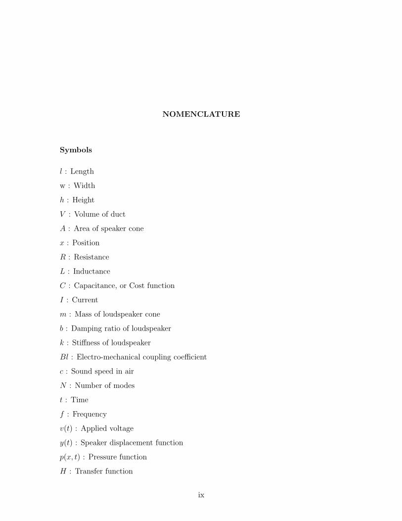
NOMENCLATURE

Symbols

l : Length

w : Width

h : Height

V : Volume of duct

A : Area of speaker cone

x : Position

R : Resistance

L : Inductance

C : Capacitance, or Cost function

I : Current

m : Mass of loudspeaker cone

b : Damping ratio of loudspeaker

k : Stiffness of loudspeaker

Bl : Electro-mechanical coupling coefficient

c : Sound speed in air

N : Number of modes

t : Time

f : Frequency

v(t) : Applied voltage

y(t) : Speaker displacement function

p(x, t) : Pressure function

H : Transfer function

ix

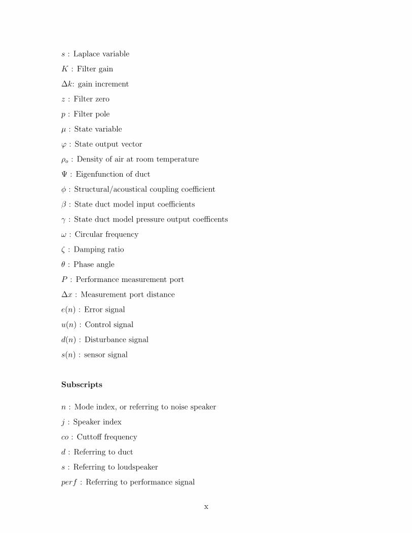
s : Laplace variable

K : Filter gain

∆k: gain increment

z : Filter zero

p : Filter pole

µ : State variable

ϕ : State output vector

ρo : Density of air at room temperature

Ψ : Eigenfunction of duct

φ : Structural/acoustical coupling coefficient

β : State duct model input coefficients

γ : State duct model pressure output coefficents

ω : Circular frequency

ζ : Damping ratio

θ : Phase angle

P : Performance measurement port

∆x : Measurement port distance

e(n) : Error signal

u(n) : Control signal

d(n) : Disturbance signal

s(n) : sensor signal

Subscripts

n : Mode index, or referring to noise speaker

j : Speaker index

co : Cuttoff frequency

d : Referring to duct

s : Referring to loudspeaker

perf : Referring to performance signal

x

sen : Referring to sensor signal

dist : Referring to disturbance signal

cont : Referring to control signal

dp : Referring to distrubance/performance path

ds : Referring to distrubance/sensor path

cs : Referring to control/sensor path

cp : Referring to control/performance path

c : Referring to control speaker

comp : Referring to the compensator

f : Referring to generic filter

a : Referring to all-pass filter

g : Referring to gain circuit

LP : Low-pass filter

BP : Band-pass filter

AP : All-pass filter

Superscripts

˙ : First derivative, ddt

¨: Second Derivative, d2

dt2

xi

1.0 INTRODUCTION

There are two distinct means to abate unwanted sound, passive and active. Passive noise

control can be accomplished by adding absorptive treatments to surfaces, or fabricating bar-

riers or enclosures. For example, foam insulation and ceiling tiles have become features at

many offices to dissipate or disrupt the reflection of the sound field. The size and density

of passive treatments are dependent upon the acoustic wavelength, making them ideal for

middle to high frequency noise applications. Active Noise Control (ANC) uses the princi-

ple of destructive interference of waves to attenuate undesired noise. An acoustic actuator

(loudspeaker) is used to produce a signal that is “out of phase” with the disturbance. Active

approaches work best when the wavelength is long compared to the dimensions of its sur-

roundings, i.e. low frequencies noise in a waveguide. Both passive and active noise control

can be used individually, or to complement one another [1, 18].

An exception to passive devices not working well at low frequencies is the Helmholtz

resonator. For example, when the dimensions of an acoustic system are small in comparison

to the wavelength of the disturbance, the motion of the medium is analogous to lumped

parameter mechanical system [17]. The enclosed volume of air acts as a spring connected

to the mass of the slug of air, and vibrates at a frequency dependent on the density and

volume of the air and the mass of the slug of air in the neck. To obtain noise suppression,

the natural frequency of the device is tuned to match the targeted control frequency. The

radiation of sound into the surrounding medium leads to the dissipation of acoustic energy,

which acts as resistance element at the opening. Helmholtz resonators can be used to remove

energy at single or multiple frequencies. These devices have been implemented in a host of

applications, such as buildings, acoustic barriers, rocket fairings, and mufflers. The damping

of a Helmholtz resonator, much like vibration absorbers, determines the amount of control

1

that is to be expected [5, 8]. Due to the sensitivity of acoustic systems, a disadvantage

of using these devices is their inability to modify the fixed natural frequency. Approaches

have been developed to physically adapt the mechanical tuning of Helmholtz resonators

[15, 18, 25]. However, due to the active component implementing the tuning of the resonator,

these methods can be unwieldily and have physical limitations.

There are two distinct approaches to ANC: feedforward and feedback. Feedforward

control uses a coherent reference to form the control signal that drives an acoustic actuator.

Most feedforward techniques employ an adaptive algorithm, where the performance of the

controller is measured by an error sensor. This measurement provides a signal that an

algorithm uses to update the controller. For example, a least-mean-square (LMS) algorithm

updates the coefficients of a finite impulse response (FIR) filter controller to minimize mean-

squared error. An inherent requirement of feedforward systems is that the signal processing

time be less than the time it takes sound to propagate from the reference to the error sensor

[14]. It should be noted that as the error signal is minimized, higher gains will be required

for the controller, making a less stable system. Despite these drawbacks feedforward ANC

is a widely applicable control system arrangement that has shown great ability to attenuate

disturbances [25, 26].

While feedforward systems require a knowledge of the incoming disturbance to gener-

ate an ”anti-noise” signal, feedback systems attenuate the disturbance as it occurs. Thus,

feedback approaches are often better at diminishing transient events. Feedback approaches

change the system response by adding damping and modifying the resonant frequencies. A

feedback control scheme uses a sensor to detect the disturbance, and formulates a suitable

control signal that drives a loudspeaker. The best known example of feedback ANC is active

ear muffs (or active headset) [11]. The acoustic disturbance is attenuated at a microphone

inside the headset, effectively creating a zone of silence at the user’s ear. It is required that

the location of the disturbance sensor be in close proximity to the acoustic actuator for

feedback systems. The distance between actuator and sensor determines the system delay,

which is proportional to the effective bandwidth of the controller [14].

Vibrating structures, as with acoustic systems, have modes in which vibration occurs,

and the strongest oscillation occurs at the systems resonant frequencies. Although similar

2

in some respects, feedback control of structural and acoustic systems have important differ-

ences. Structural feedback systems can achieve perfect collocation between the sensor and

actuator pair [9], whereas acoustic feedback systems can not [3]. The sensor (microphone)

and actuator (loudspeaker) for acoustic systems can only achieve a “substantially collocated”

transducer pair, by placing the sensor at the center of the loudspeaker’s face. However, the

loudspeaker adds significant dynamics to the system which can cause instability and erode

controller performance.

An unconventional yet simple control approach that is used for large space structures is

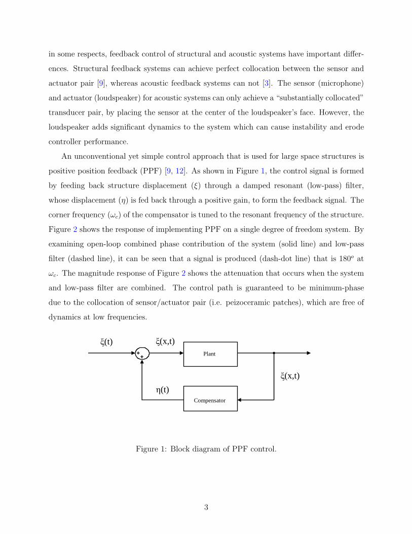
positive position feedback (PPF) [9, 12]. As shown in Figure 1, the control signal is formed

by feeding back structure displacement (ξ) through a damped resonant (low-pass) filter,

whose displacement (η) is fed back through a positive gain, to form the feedback signal. The

corner frequency (ωc) of the compensator is tuned to the resonant frequency of the structure.

Figure 2 shows the response of implementing PPF on a single degree of freedom system. By

examining open-loop combined phase contribution of the system (solid line) and low-pass

filter (dashed line), it can be seen that a signal is produced (dash-dot line) that is 180o at

ωc. The magnitude response of Figure 2 shows the attenuation that occurs when the system

and low-pass filter are combined. The control path is guaranteed to be minimum-phase

due to the collocation of sensor/actuator pair (i.e. peizoceramic patches), which are free of

dynamics at low frequencies.

Plant

Compensator

++++++++

ξ(t) ξ(x,t)

η(t)

ξ(x,t)

Figure 1: Block diagram of PPF control.

3

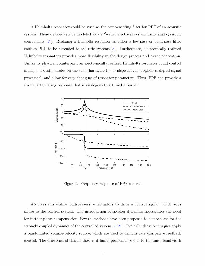
A Helmholtz resonator could be used as the compensating filter for PPF of an acoustic

system. These devices can be modeled as a 2nd-order electrical system using analog circuit

components [17]. Realizing a Helmoltz resonator as either a low-pass or band-pass filter

enables PPF to be extended to acoustic systems [3]. Furthermore, electronically realized

Helmholtz resonators provides more flexibility in the design process and easier adaptation.

Unlike its physical counterpart, an electronically realized Helmholtz resonator could control

multiple acoustic modes on the same hardware (i.e loudspeaker, microphones, digital signal

processor), and allow for easy changing of resonator parameters. Thus, PPF can provide a

stable, attenuating response that is analogous to a tuned absorber.

−60

−40

−20

0

20

40

Mag

nitu

de (

dB)

20 40 60 80 100 120 140 160 180 200−360

−270

−180

−90

0

Pha

se (

deg)

Frequency (Hz)

Plant

Compensator

Open−Loop

ωc

Figure 2: Frequency response of PPF control.

ANC systems utilize loudspeakers as actuators to drive a control signal, which adds

phase to the control system. The introduction of speaker dynamics necessitates the need

for further phase compensation. Several methods have been proposed to compensate for the

strongly coupled dynamics of the controlled system [2, 21]. Typically these techniques apply

a band-limited volume-velocity source, which are used to demonstrate dissipative feedback

control. The drawback of this method is it limits performance due to the finite bandwidth

4

of the compensating loudspeaker. Another possibility is to use an all-pass phase correction

filter in congruence with a resonant filter [3].

Research using resonant filters to control acoustic plants is limited, but has been shown

to work well. The inherent limitations of these methods is the inability to perfectly collocate

the sensor/actuator pair, thus allowing loudspeaker dynamics to diminish performance and

stability. One report presented a procedure where the low-frequency modes of the plant were

ignored, effectively allowing the phase induced by the speaker not to destabilize and erode

performance on the controller [10]. Another report demonstrated a pacifying control system

that utilized a feed through term for non-collocated control. However, global control was not

addressed due to the sensor and error location being the same [27]. By using an all-pass filter

design scheme in conjunction with PPF, global control is permitted at any sensor location.

This compensation method eases the collocation requirement on the sensor/actuator pair,

giving greater tolerance to the type and location of control transducer used.

Many variations of PPF can be achieved given the inherent forgiveness of high-frequency

finite actuator dynamics [9]. However, structural PPF uses piezoelectric actuators which do

not contribute phase, in contrast acoustic PPF utilize loudspeakers that do add phase to the

system. Resonant band-pass filters, rather than low-pass filters, would be desirable when

considering multi-modal control of acoustic systems. The roll-off associated with band-pass

filters would limit interactions between adjacent modes. As long as the phase of the control

path is compensated to the desired 180o at each mode, stability margins can be maintained.

Thus, the gain is precisely focused around the targeted resonant frequency of system.

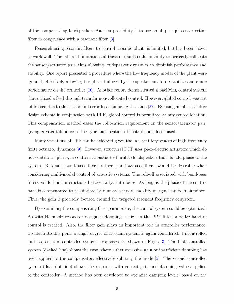
By examining the compensating filter parameters, the control system could be optimized.

As with Helmholz resonator design, if damping is high in the PPF filter, a wider band of

control is created. Also, the filter gain plays an important role in controller performance.

To illustrate this point a single degree of freedom system is again considered. Uncontrolled

and two cases of controlled systems responses are shown in Figure 3. The first controlled

system (dashed line) shows the case where either excessive gain or insufficient damping has

been applied to the compensator, effectively splitting the mode [5]. The second controlled

system (dash-dot line) shows the response with correct gain and damping values applied

to the controller. A method has been developed to optimize damping levels, based on the

5

knowledge of the dc-gain and pole-zero spacing [23]. This work showed that a phase shift of

10 degrees in the control path can deteriorate control performance by as much as 70 percent.

−20

−10

0

10

20

30

40

Mag

nitu

de (

dB)

20 40 60 80 100 120 140−180

−135

−90

−45

0

Pha

se (

deg)

Frequency (Hz)

Uncontrolled System

Controlled System 1

Controlled System 2

Figure 3: Uncontrolled and controlled frequency response of PPF control.

This study extends the achievements of using electronically realized Helmholtz resonators

in a PPF control scheme [3]. The use of resonant filters is further investigated, by examining

them in higher order models. Various types of filters are also explored (i.e. Butterworth,

Chebyshev, and elliptical) and used in congruence with all-pass filter compensation arrange-

ments. By using higher order and band-pass filters, multi-modal control becomes greatly

improved due to the embedded characteristics of the filters. Finally, an adaptive gain algo-

rithm is examined to achieve an optimized broadband multi-modal controller. Realizing the

controller electronically greatly facilitates the optimization process.

6

2.0 THEORETICAL DEVELOPMENT

2.1 ANALYTICAL DUCT MODEL

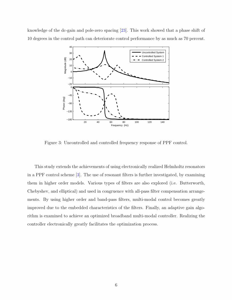
To examine the proposed feedback ANC scheme, a one-dimensional waveguide is considered.

An acoustic enclosure produces a reverberant sound field that has sparse modal shaping,

allowing for close examination of the first few modes. A schematic of the enclosure can be

seen in Figure 4. The dimensions of the duct are comprised of the length ld, width wd, and

height hd. The rigid-walled duct contains two midrange loudspeakers with a face width ws,

located at each end. One is centered at x1 and the other about x2, providing the disturbance

and control inputs, respectively. Two acoustic sensors will provide the output signals, located

at xperf and x2, which will be discussed later in Section 3.1.

ws ws

x

y

ld

x1

x2

xperf

DisturbanceLoudspeaker

ControlLoudspeaker

hd

Figure 4: Acoustic duct setup.

7

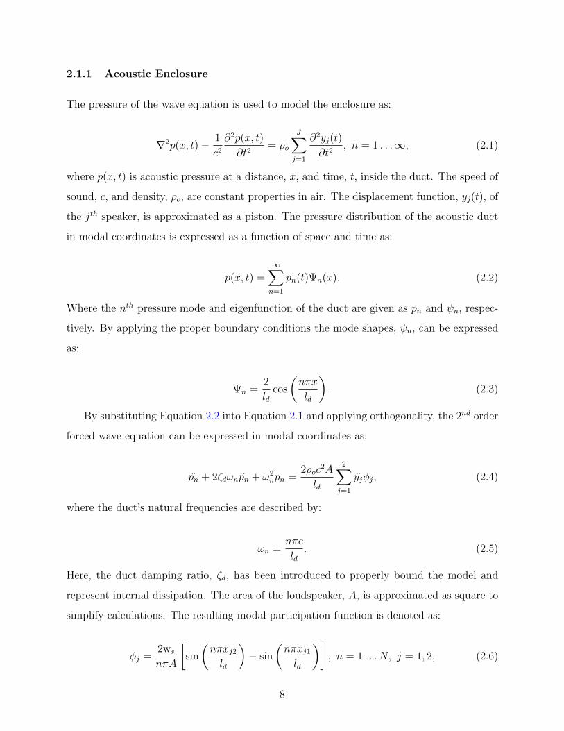
2.1.1 Acoustic Enclosure

The pressure of the wave equation is used to model the enclosure as:

∇2p(x, t)− 1

c2∂2p(x, t)

∂t2= ρo

J∑j=1

∂2yj(t)

∂t2, n = 1 . . .∞, (2.1)

where p(x, t) is acoustic pressure at a distance, x, and time, t, inside the duct. The speed of

sound, c, and density, ρo, are constant properties in air. The displacement function, yj(t), of

the jth speaker, is approximated as a piston. The pressure distribution of the acoustic duct

in modal coordinates is expressed as a function of space and time as:

p(x, t) =∞∑

n=1

pn(t)Ψn(x). (2.2)

Where the nth pressure mode and eigenfunction of the duct are given as pn and ψn, respec-

tively. By applying the proper boundary conditions the mode shapes, ψn, can be expressed

as:

Ψn =2

ldcos

(nπx

ld

). (2.3)

By substituting Equation 2.2 into Equation 2.1 and applying orthogonality, the 2nd order

forced wave equation can be expressed in modal coordinates as:

pn + 2ζdωnpn + ω2npn =

2ρoc2A

ld

2∑j=1

yjφj, (2.4)

where the duct’s natural frequencies are described by:

ωn =nπc

ld. (2.5)

Here, the duct damping ratio, ζd, has been introduced to properly bound the model and

represent internal dissipation. The area of the loudspeaker, A, is approximated as square to

simplify calculations. The resulting modal participation function is denoted as:

φj =2ws

nπA

[sin

(nπxj2

ld

)− sin

(nπxj1

ld

)], n = 1 . . . N, j = 1, 2, (2.6)

8

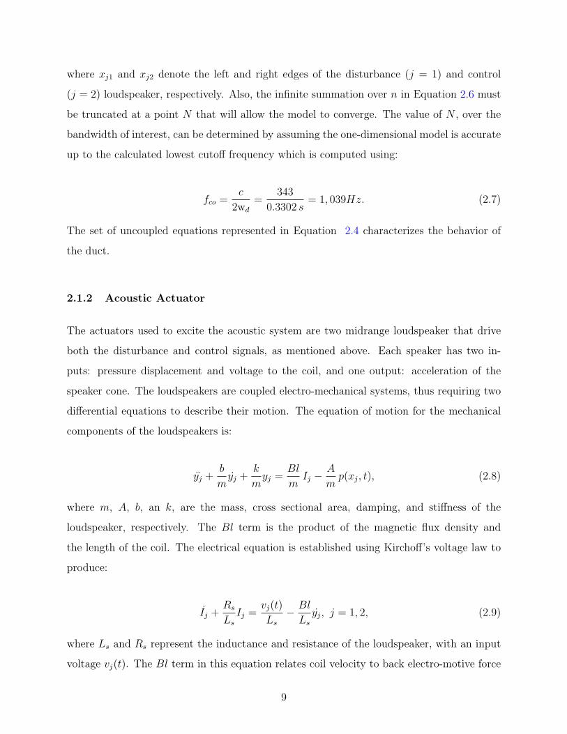
where xj1 and xj2 denote the left and right edges of the disturbance (j = 1) and control

(j = 2) loudspeaker, respectively. Also, the infinite summation over n in Equation 2.6 must

be truncated at a point N that will allow the model to converge. The value of N , over the

bandwidth of interest, can be determined by assuming the one-dimensional model is accurate

up to the calculated lowest cutoff frequency which is computed using:

fco =c

2wd

=343

0.3302 s= 1, 039Hz. (2.7)

The set of uncoupled equations represented in Equation 2.4 characterizes the behavior of

the duct.

2.1.2 Acoustic Actuator

The actuators used to excite the acoustic system are two midrange loudspeaker that drive

both the disturbance and control signals, as mentioned above. Each speaker has two in-

puts: pressure displacement and voltage to the coil, and one output: acceleration of the

speaker cone. The loudspeakers are coupled electro-mechanical systems, thus requiring two

differential equations to describe their motion. The equation of motion for the mechanical

components of the loudspeakers is:

yj +b

myj +

k

myj =

Bl

mIj −

A

mp(xj, t), (2.8)

where m, A, b, an k, are the mass, cross sectional area, damping, and stiffness of the

loudspeaker, respectively. The Bl term is the product of the magnetic flux density and

the length of the coil. The electrical equation is established using Kirchoff’s voltage law to

produce:

Ij +Rs

Ls

Ij =vj(t)

Ls

− Bl

Ls

yj, j = 1, 2, (2.9)

where Ls and Rs represent the inductance and resistance of the loudspeaker, with an input

voltage vj(t). The Bl term in this equation relates coil velocity to back electro-motive force

9

(EMF). The above equations are used to produce a coupled acousto/mechanical equation

[3], written in modal form as:

yj +b

myj +

k

myj =

Bl

mIj −

A

m

N∑n=1

pn(t)φj, j = 1, 2. (2.10)

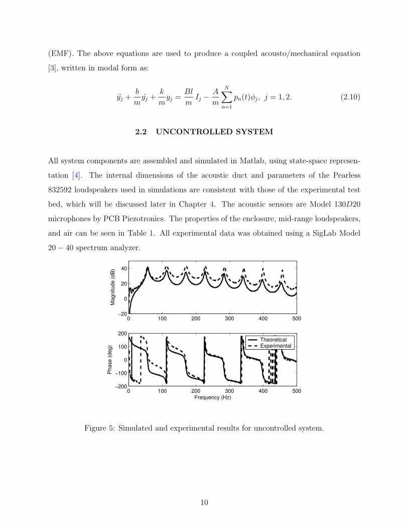
2.2 UNCONTROLLED SYSTEM

All system components are assembled and simulated in Matlab, using state-space represen-

tation [4]. The internal dimensions of the acoustic duct and parameters of the Pearless

832592 loudspeakers used in simulations are consistent with those of the experimental test

bed, which will be discussed later in Chapter 4. The acoustic sensors are Model 130D20

microphones by PCB Piezotronics. The properties of the enclosure, mid-range loudspeakers,

and air can be seen in Table 1. All experimental data was obtained using a SigLab Model

20− 40 spectrum analyzer.

0 100 200 300 400 500−20

0

20

40

Mag

nitu

de (d

B)

0 100 200 300 400 500−200

−100

0

100

200

Pha

se (d

eg)

Frequency (Hz)

TheoreticalExperimental

Figure 5: Simulated and experimental results for uncontrolled system.

10

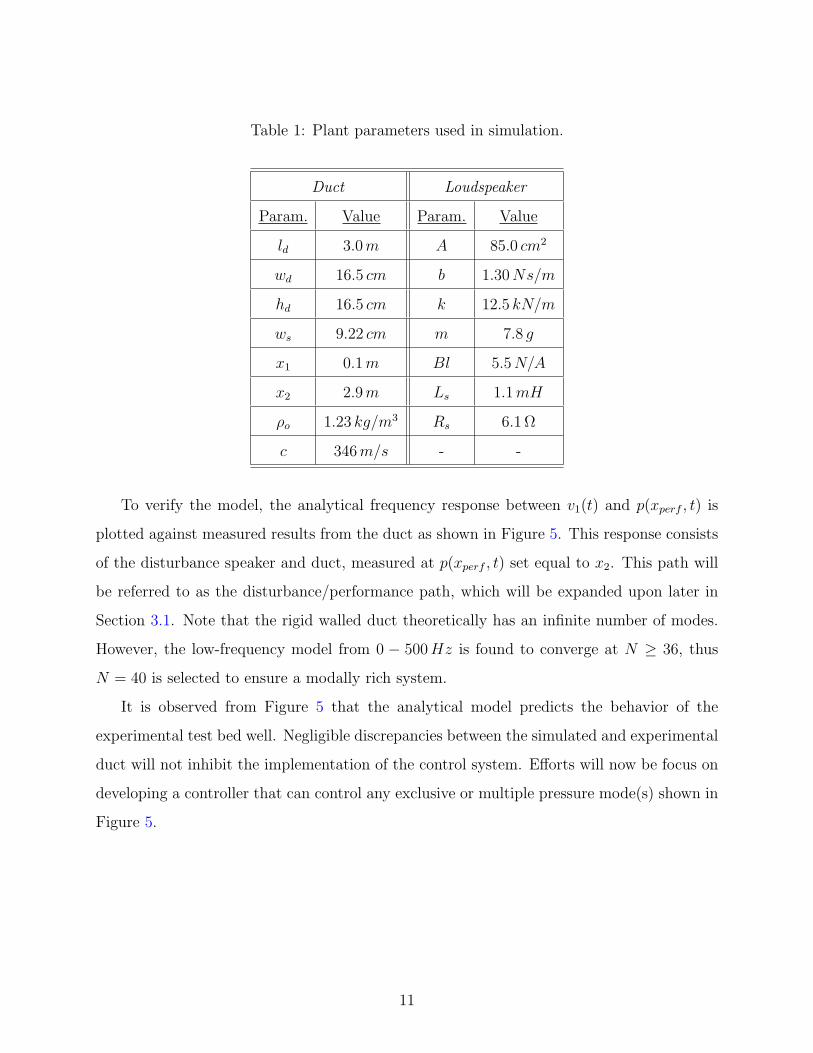
Table 1: Plant parameters used in simulation.

Duct Loudspeaker

Param. Value Param. Value

ld 3.0m A 85.0 cm2

wd 16.5 cm b 1.30Ns/m

hd 16.5 cm k 12.5 kN/m

ws 9.22 cm m 7.8 g

x1 0.1m Bl 5.5N/A

x2 2.9m Ls 1.1mH

ρo 1.23 kg/m3 Rs 6.1 Ω

c 346m/s - -

To verify the model, the analytical frequency response between v1(t) and p(xperf , t) is

plotted against measured results from the duct as shown in Figure 5. This response consists

of the disturbance speaker and duct, measured at p(xperf , t) set equal to x2. This path will

be referred to as the disturbance/performance path, which will be expanded upon later in

Section 3.1. Note that the rigid walled duct theoretically has an infinite number of modes.

However, the low-frequency model from 0 − 500Hz is found to converge at N ≥ 36, thus

N = 40 is selected to ensure a modally rich system.

It is observed from Figure 5 that the analytical model predicts the behavior of the

experimental test bed well. Negligible discrepancies between the simulated and experimental

duct will not inhibit the implementation of the control system. Efforts will now be focus on

developing a controller that can control any exclusive or multiple pressure mode(s) shown in

Figure 5.

11

3.0 CONTROL SIMULATION

A compensator that will attenuate the resonant modes of the duct is developed and discussed

in this chapter. The adopted control scheme is similar to PPF used for structures, but has

been extended to acoustic systems [3, 29]. A collocated sensor/actuator pair produces a ref-

erence pressure that is fed back through a tuned compensating filter to produce a signal that

is 180o out of phase with the input signal at the control frequency, ωc. Loudspeaker actuator

dynamics add phase to the system, which is not observed in structural PPF examples [9, 12].

These undesired dynamics are compensated for by employing an all-pass filter in series with

the magnitude-shaping filter [3, 4].

The achievements made by prior acoustic PPF studies is extended through examina-

tion of analytical simulations [29]. Previously, only modest attempts at multi-modal control

have been attempted. Phase interactions between uncontrolled and controlled duct modes

is examined for both single and multi-modal cases. Compensator damping determines the

amount of phase interaction that will occur between modes, due to resonant filter roll-off.

Different types of higher-order filters are investigated to improve controller performance.

To gain greater insight into controller stability and performance, Nyquist stability is exam-

ined, as opposed to root-locus stability analysis. Realizing the control system electronically,

through a digital signal processor (DSP), allows for easy implementation of higher-order

filters. The DSP board also permits the multi-modal controller to use the same hardware

(i.e. DSP, loudspeaker, and microphones), and facilitates the examination of compensator

design variables.

In this chapter, control system modifications are simulated on the analytical duct model.

The transfer function paths associated with the control system configuration are examined. A

single mode controller is developed, which consists of a resonant magnitude-shaping filter and

12

a phase-correction filter. Effects of modifying the resonant filter damping, order, and design-

type are investigated. The procedure is then extended to the design and demonstration of

the a multi-modal controller.

3.1 CONTROL SYSTEM CONFIGURATION

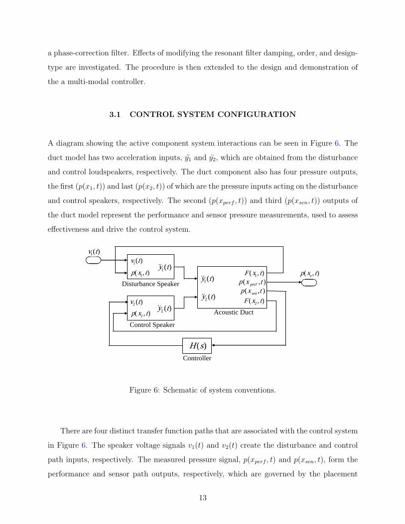
A diagram showing the active component system interactions can be seen in Figure 6. The

duct model has two acceleration inputs, y1 and y2, which are obtained from the disturbance

and control loudspeakers, respectively. The duct component also has four pressure outputs,

the first (p(x1, t)) and last (p(x2, t)) of which are the pressure inputs acting on the disturbance

and control speakers, respectively. The second (p(xperf , t)) and third (p(xsen, t)) outputs of

the duct model represent the performance and sensor pressure measurements, used to assess

effectiveness and drive the control system.

)(1 ty&&

)(1 tv

),( txp perf

Control Speaker

Disturbance Speaker

Acoustic Duct

),( 1 txF

),( txp sen

),( 2 txF

),( 1 txp)(1 ty&&

)(2 ty&&

),( txp e

)(2 ty&&),( 2 txp

)(1 tv

)(2 tv

)(sHController

Figure 6: Schematic of system conventions.

There are four distinct transfer function paths that are associated with the control system

in Figure 6. The speaker voltage signals v1(t) and v2(t) create the disturbance and control

path inputs, respectively. The measured pressure signal, p(xperf , t) and p(xsen, t), form the

performance and sensor path outputs, respectively, which are governed by the placement

13

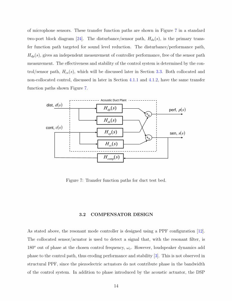
of microphone sensors. These transfer function paths are shown in Figure 7 in a standard

two-port block diagram [24]. The disturbance/sensor path, Hds(s), is the primary trans-

fer function path targeted for sound level reduction. The disturbance/performance path,

Hdp(s), gives an independent measurement of controller performance, free of the sensor path

measurement. The effectiveness and stability of the control system is determined by the con-

trol/sensor path, Hcs(s), which will be discussed later in Section 3.3. Both collocated and

non-collocated control, discussed in later in Section 4.1.1 and 4.1.2, have the same transfer

function paths shown Figure 7.

)(sHcp

)(sHcs

)(sHds

)(sHdp

)(sHcomp

++

++

cont,

dist, perf,

sen,

Acoustic Duct Plant

( )sd

( )sc

( )sp

( )ss

Figure 7: Transfer function paths for duct test bed.

3.2 COMPENSATOR DESIGN

As stated above, the resonant mode controller is designed using a PPF configuration [12].

The collocated sensor/acuator is used to detect a signal that, with the resonant filter, is

180o out of phase at the chosen control frequency, ωc. However, loudspeaker dynamics add

phase to the control path, thus eroding performance and stability [3]. This is not observed in

structural PPF, since the piezoelectric actuators do not contribute phase in the bandwidth

of the control system. In addition to phase introduced by the acoustic actuator, the DSP

14

board that is used to implement the resonant filter also contributes phase to the system [29].

Thus, a digital version of the all-pass filter network is used to compensate for these phase

shifts. The acoustic resonant mode controller consists of either a band-pass or low-pass filter,

and a phase-correcting all-pass filter.

In this section, a compensating filter network, Hcomp(s), that will produce the control

signal is designed. For a stable closed-loop feedback system, it is desired that the phase at

the targeted frequency, ωc, be ±180o. For a the two-port system shown in Figure 7, the

phase at the control frequency is found by examining the control/sensor path, Hcs(s). The

total phase at the compensator is described by:

θc(ωc) = θf (ωc) + θa(ωc) = θs(ωc) + θd(ωc) + θdsp(ωc). (3.1)

The phase contribution is constant for loudspeakers, θs(ωc), duct, θd(ωc), and unit sample

delay from the DSP, θdsp(ωc). The phase induced by the resonant filters in the controller,

θf (ωc), are 90o for low-pass filters and 0o for band-pass filters. Thus, some form of fine-tuning

phase adjustment will be required, due to phase added to the control/sensor path. This is

achieved through implementing an all-pass filter [3], via the θa(ωc) term in Equation 3.1,

which be discussed later in Section 3.2.2.

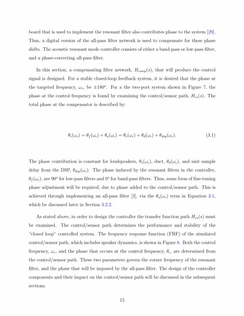
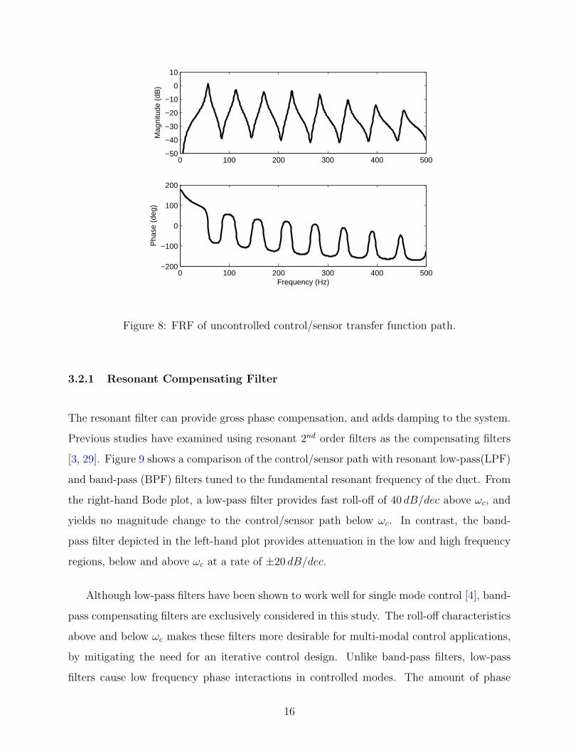
As stated above, in order to design the controller the transfer function path Hcs(s) must

be examined. The control/sensor path determines the performance and stability of the

“closed loop” controlled system. The frequency response function (FRF) of the simulated

control/sensor path, which includes speaker dynamics, is shown in Figure 8. Both the control

frequency, ωc, and the phase that occurs at the control frequency, θc, are determined from

the control/sensor path. These two parameters govern the corner frequency of the resonant

filter, and the phase that will be imposed by the all-pass filter. The design of the controller

components and their impact on the control/sensor path will be discussed in the subsequent

sections.

15

0 100 200 300 400 500−50

−40

−30

−20

−10

0

10

Mag

nitu

de (

dB)

0 100 200 300 400 500−200

−100

0

100

200

Pha

se (

deg)

Frequency (Hz)

Figure 8: FRF of uncontrolled control/sensor transfer function path.

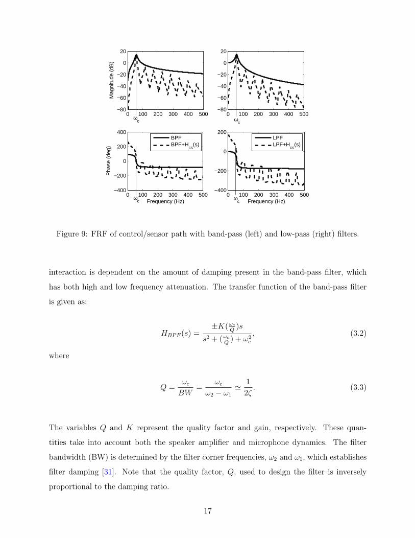
3.2.1 Resonant Compensating Filter

The resonant filter can provide gross phase compensation, and adds damping to the system.

Previous studies have examined using resonant 2nd order filters as the compensating filters

[3, 29]. Figure 9 shows a comparison of the control/sensor path with resonant low-pass(LPF)

and band-pass (BPF) filters tuned to the fundamental resonant frequency of the duct. From

the right-hand Bode plot, a low-pass filter provides fast roll-off of 40 dB/dec above ωc, and

yields no magnitude change to the control/sensor path below ωc. In contrast, the band-

pass filter depicted in the left-hand plot provides attenuation in the low and high frequency

regions, below and above ωc at a rate of ±20 dB/dec.

Although low-pass filters have been shown to work well for single mode control [4], band-

pass compensating filters are exclusively considered in this study. The roll-off characteristics

above and below ωc makes these filters more desirable for multi-modal control applications,

by mitigating the need for an iterative control design. Unlike band-pass filters, low-pass

filters cause low frequency phase interactions in controlled modes. The amount of phase

16

0 100 200 300 400 500−80

−60

−40

−20

0

20

Mag

nitu

de (

dB)

0 100 200 300 400 500−400

−200

0

200

400

Pha

se (

deg)

Frequency (Hz)

BPFBPF+H

cs(s)

0 100 200 300 400 500−80

−60

−40

−20

0

20

0 100 200 300 400 500−400

−200

0

200

Frequency (Hz)

LPFLPF+H

cs(s)

ωc

ωc

ωc

ωc

Figure 9: FRF of control/sensor path with band-pass (left) and low-pass (right) filters.

interaction is dependent on the amount of damping present in the band-pass filter, which

has both high and low frequency attenuation. The transfer function of the band-pass filter

is given as:

HBPF (s) =±K(ωc

Q)s

s2 + (ωc

Q) + ω2

c

, (3.2)

where

Q =ωc

BW=

ωc

ω2 − ω1

' 1

2ζ. (3.3)

The variables Q and K represent the quality factor and gain, respectively. These quan-

tities take into account both the speaker amplifier and microphone dynamics. The filter

bandwidth (BW) is determined by the filter corner frequencies, ω2 and ω1, which establishes

filter damping [31]. Note that the quality factor, Q, used to design the filter is inversely

proportional to the damping ratio.

17

−30

−20

−10

0

10

20

Mag

nitu

de (

dB)

101

102

103

−90

−45

0

45

90

Pha

se (

deg)

Frequency (rad/sec)

ζ = 0.1

ζ = 0.4

ζ = 0.7

ζ = 1

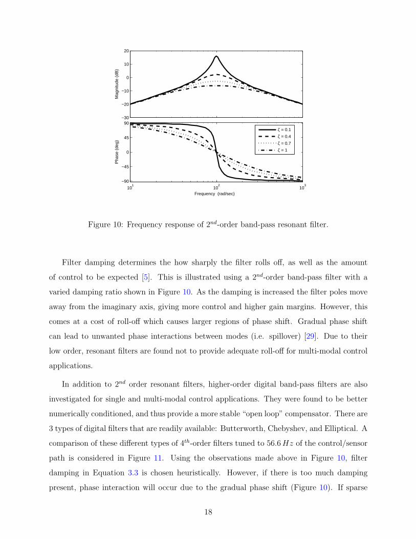
Figure 10: Frequency response of 2nd-order band-pass resonant filter.

Filter damping determines the how sharply the filter rolls off, as well as the amount

of control to be expected [5]. This is illustrated using a 2nd-order band-pass filter with a

varied damping ratio shown in Figure 10. As the damping is increased the filter poles move

away from the imaginary axis, giving more control and higher gain margins. However, this

comes at a cost of roll-off which causes larger regions of phase shift. Gradual phase shift

can lead to unwanted phase interactions between modes (i.e. spillover) [29]. Due to their

low order, resonant filters are found not to provide adequate roll-off for multi-modal control

applications.

In addition to 2nd order resonant filters, higher-order digital band-pass filters are also

investigated for single and multi-modal control applications. They were found to be better

numerically conditioned, and thus provide a more stable “open loop” compensator. There are

3 types of digital filters that are readily available: Butterworth, Chebyshev, and Elliptical. A

comparison of these different types of 4th-order filters tuned to 56.6Hz of the control/sensor

path is considered in Figure 11. Using the observations made above in Figure 10, filter

damping in Equation 3.3 is chosen heuristically. However, if there is too much damping

present, phase interaction will occur due to the gradual phase shift (Figure 10). If sparse

18

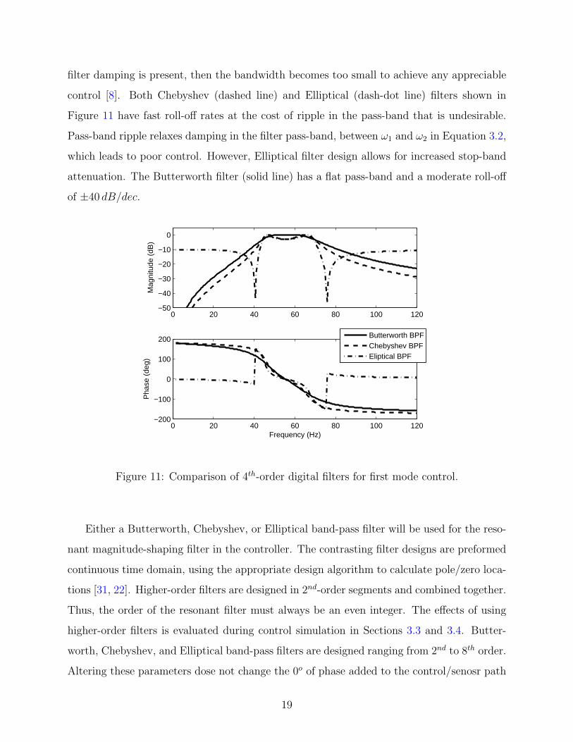
filter damping is present, then the bandwidth becomes too small to achieve any appreciable

control [8]. Both Chebyshev (dashed line) and Elliptical (dash-dot line) filters shown in

Figure 11 have fast roll-off rates at the cost of ripple in the pass-band that is undesirable.

Pass-band ripple relaxes damping in the filter pass-band, between ω1 and ω2 in Equation 3.2,

which leads to poor control. However, Elliptical filter design allows for increased stop-band

attenuation. The Butterworth filter (solid line) has a flat pass-band and a moderate roll-off

of ±40 dB/dec.

0 20 40 60 80 100 120−50

−40

−30

−20

−10

0

Mag

nitu

de (

dB)

0 20 40 60 80 100 120−200

−100

0

100

200

Pha

se (

deg)

Frequency (Hz)

Butterworth BPFChebyshev BPFEliptical BPF

Figure 11: Comparison of 4th-order digital filters for first mode control.

Either a Butterworth, Chebyshev, or Elliptical band-pass filter will be used for the reso-

nant magnitude-shaping filter in the controller. The contrasting filter designs are preformed

continuous time domain, using the appropriate design algorithm to calculate pole/zero loca-

tions [31, 22]. Higher-order filters are designed in 2nd-order segments and combined together.

Thus, the order of the resonant filter must always be an even integer. The effects of using

higher-order filters is evaluated during control simulation in Sections 3.3 and 3.4. Butter-

worth, Chebyshev, and Elliptical band-pass filters are designed ranging from 2nd to 8th order.

Altering these parameters dose not change the 0o of phase added to the control/senosr path

19

by the band-pass filter at ωc, and compensator design for remains unchanged for single mode

control. However, all parallel connected band-pass filters must be taken into account when

designing a multi-modal controller due to phase interactions above and below ωc. Whether

attempting single or multiple mode control, the phase induced by the loudspeaker and DSP

still need to be accounted for in order to achieve the control signal.

3.2.2 Phase Compensation

Although the single-mode, band-pass compensating filter contributes no phase to the con-

trol/sensor path, the phase introduced by the loudspeaker needs to be accounted for [3]. In

order to achieve a control signal that is perfectly out of phase, an all-pass phase correction

filter is employed [4]. The all-pass filter has no adverse impacts on the magnitude of the con-

trol paths. Thus, the achievements made by the band-pass filter are not effected. However,

when attempting multi-modal control phase shifts are introduced by the parallel connection

of the resonant filters. The phase induced by multi-modal control can still be accounted for

with the use of the all-pass filter phase correction scheme, due to the damping added to the

compensator by the band-pass filter.

An all-pass filter can provide a non-inverting phase shift ranging from 0o − 180o, and an

inverting phase shift of 180o−360o. The phase shift required of the all-pass filter is dependent

upon the phase present at the control path targeted frequency. The Laplace transfer function

of the all-pass filter is expressed as:

HAP (s) =±(s− z)

s+ p, (3.4)

where, z and p are the locations of the all-pass filter zero and pole, respectively. The phase

angle required of the all-pass filter is determined by rearranging Equation 3.1 as:

θa = 180− θc(ωc) = θf (ωc) + θs(ωc) + θd(ωc) + θdsp(ωc). (3.5)

The phase at the control frequency in Equation 3.5 is subtracted by 180o to find the all-pass

filter phase contribution . Note that θc(ωc) could be any angle between 0o and 360o, and the

20

phase contribution for all other system components is constant. Thus, both inverting and

non-inverting all-pass filter pole/zero locations are determined by:

p = z =

ωc

cot(πθa360

)if 0o < θa ≤ 180o,

− ωc

tan(πθa360

)if 180o < θa ≤ 360o.

(3.6)

The all-pass filter is created using the pole/zero found in Equation 3.6 and substituted into

the transfer function in Equation 3.4. Once the all-pass filter is designed, it is combined in

series connection with the magnitude shaping filter described in Section 3.2.1. The compen-

sator (BPF + APF) will produce a signal that is 180o out of phase at ωc on the control/sensor

path.

3.3 SINGLE MODE CONTROL

A control system that can control any single mode, will be demonstrated on the analytical

duct model. The controller consists of a band-pass filter and a phase-compensating all-pass

filter. The control frequency, ωc, along with the control phase angle, θc, are chosen from

the uncontrolled control/sensor path in Figure 8. Equation 3.5 is then used to calculate the

phase required of the all-pass filter. Both disturbance paths, Hdp(s) and Hds(s) in Figure

8, will be used to evaluate the performance of the controller. Control of a single duct mode

will first be considered here, and the procedure will be extended to the multi-modal case in

the next section.

A single mode controller is developed using the components described in Sections 3.2.1

and 3.2.2. The first pressure node of 56.6Hz is targeted for control. In examining Figure

8, it is realized that θc(ωc) = 4o for the fundamental duct mode. Thus, from Equation

3.5, the all-pass filter must provide a non-inverting phase angle of 176o. The single-mode

compensator consists of a resonant magnitude-shaping filter with a band-width of 30Hz,

tuned to the first mode, placed in series with an all-pass filter.

As stated above, the stability and performance of the system is determined by the con-

trol/sensor path. In order to establish the gain to be applied to the compensator, standard

21

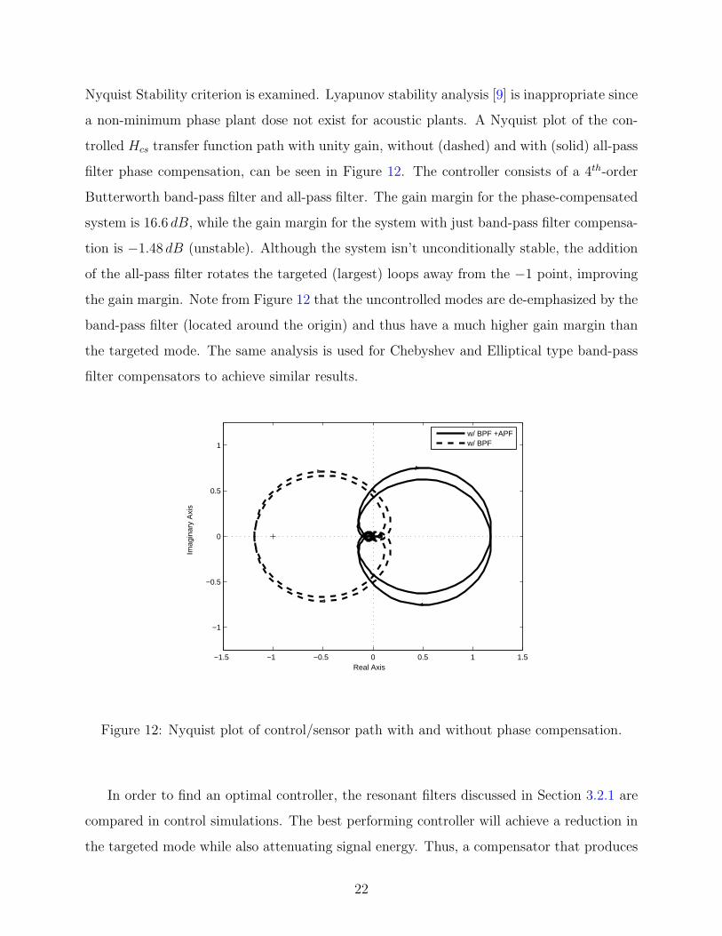
Nyquist Stability criterion is examined. Lyapunov stability analysis [9] is inappropriate since

a non-minimum phase plant dose not exist for acoustic plants. A Nyquist plot of the con-

trolled Hcs transfer function path with unity gain, without (dashed) and with (solid) all-pass

filter phase compensation, can be seen in Figure 12. The controller consists of a 4th-order

Butterworth band-pass filter and all-pass filter. The gain margin for the phase-compensated

system is 16.6 dB, while the gain margin for the system with just band-pass filter compensa-

tion is −1.48 dB (unstable). Although the system isn’t unconditionally stable, the addition

of the all-pass filter rotates the targeted (largest) loops away from the −1 point, improving

the gain margin. Note from Figure 12 that the uncontrolled modes are de-emphasized by the

band-pass filter (located around the origin) and thus have a much higher gain margin than

the targeted mode. The same analysis is used for Chebyshev and Elliptical type band-pass

filter compensators to achieve similar results.

−1.5 −1 −0.5 0 0.5 1 1.5

−1

−0.5

0

0.5

1

Real Axis

Imag

inar

y A

xis

w/ BPF +APFw/ BPF

Figure 12: Nyquist plot of control/sensor path with and without phase compensation.

In order to find an optimal controller, the resonant filters discussed in Section 3.2.1 are

compared in control simulations. The best performing controller will achieve a reduction in

the targeted mode while also attenuating signal energy. Thus, a compensator that produces

22

spill-over due to adjacent mode phase interactions will be observed as poor control. Using

signal energy as a measure of control system performance allows for adaptation of system

parameters, discussed in Chapter 5. Each controller is designed as described above, but the

type and order of the resonant filter is varied. Compensator damping is chosen heuristically,

which remains the same for all cases. A different gain is used for each case, by dividing

the gain margin in half. However, this guarantees that the stability is the same for all

compensator designs.

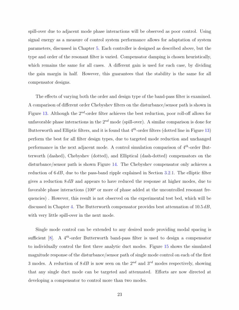
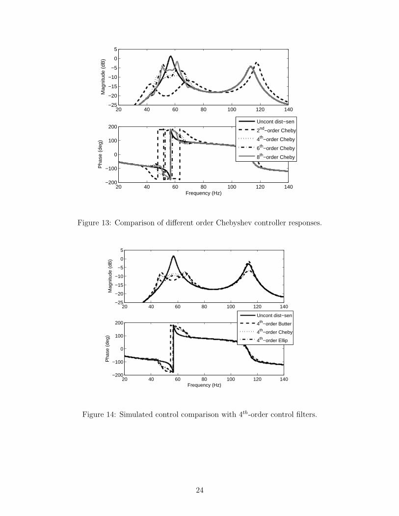
The effects of varying both the order and design type of the band-pass filter is examined.

A comparison of different order Chebyshev filters on the disturbance/sensor path is shown in

Figure 13. Although the 2nd-order filter achieves the best reduction, poor roll-off allows for

unfavorable phase interactions in the 2nd mode (spill-over). A similar comparison is done for

Butterworth and Elliptic filters, and it is found that 4th-order filters (dotted line in Figure 13)

perform the best for all filter design types, due to targeted mode reduction and unchanged

performance in the next adjacent mode. A control simulation comparison of 4th-order But-

terworth (dashed), Chebyshev (dotted), and Elliptical (dash-dotted) compensators on the

disturbance/sensor path is shown Figure 14. The Chebyshev compensator only achieves a

reduction of 6 dB, due to the pass-band ripple explained in Section 3.2.1. The elliptic filter

gives a reduction 8 dB and appears to have reduced the response at higher modes, due to

favorable phase interactions (100o or more of phase added at the uncontrolled resonant fre-

quencies) . However, this result is not observed on the experimental test bed, which will be

discussed in Chapter 4. The Butterworth compensator provides best attenuation of 10.5 dB,

with very little spill-over in the next mode.

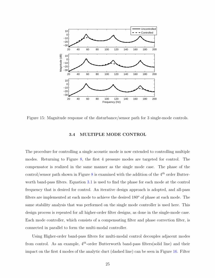
Single mode control can be extended to any desired mode providing modal spacing is

sufficient [8]. A 4th-order Butterworth band-pass filter is used to design a compensator

to individually control the first three analytic duct modes. Figure 15 shows the simulated

magnitude response of the disturbance/sensor path of single mode control on each of the first

3 modes. A reduction of 8 dB is now seen on the 2nd and 3rd modes respectively, showing

that any single duct mode can be targeted and attenuated. Efforts are now directed at

developing a compensator to control more than two modes.

23

20 40 60 80 100 120 140−25

−20

−15

−10

−5

0

5

Mag

nitu

de (

dB)

20 40 60 80 100 120 140−200

−100

0

100

200

Pha

se (

deg)

Frequency (Hz)

Uncont dist−sen

2nd−order Cheby

4th−order Cheby

6th−order Cheby

8th−order Cheby

Figure 13: Comparison of different order Chebyshev controller responses.

20 40 60 80 100 120 140−25

−20

−15

−10

−5

0

5

Mag

nitu

de (

dB)

20 40 60 80 100 120 140−200

−100

0

100

200

Pha

se (

deg)

Frequency (Hz)

Uncont dist−sen

4th−order Butter

4th−order Cheby

4th−order Ellip

Figure 14: Simulated control comparison with 4th-order control filters.

24

20 40 60 80 100 120 140 160 180 200

−30−20−10

010

UncontrolledControlled

20 40 60 80 100 120 140 160 180 200

−30−20−10

010

Mag

nitu

de (

dB)

20 40 60 80 100 120 140 160 180 200

−30−20−10

010

Frequency (Hz)

Figure 15: Magnitude response of the disturbance/sensor path for 3 single-mode controls.

3.4 MULTIPLE MODE CONTROL

The procedure for controlling a single acoustic mode is now extended to controlling multiple

modes. Returning to Figure 8, the first 4 pressure modes are targeted for control. The

compensator is realized in the same manner as the single mode case. The phase of the

control/sensor path shown in Figure 8 is examined with the addition of the 4th order Butter-

worth band-pass filters. Equation 3.1 is used to find the phase for each mode at the control

frequency that is desired for control. An iterative design approach is adopted, and all-pass

filters are implemented at each mode to achieve the desired 180o of phase at each mode. The

same stability analysis that was performed on the single mode controller is used here. This

design process is repeated for all higher-order filter designs, as done in the single-mode case.

Each mode controller, which consists of a compensating filter and phase correction filter, is

connected in parallel to form the multi-modal controller.

Using Higher-order band-pass filters for multi-modal control decouples adjacent modes

from control. As an example, 4th-order Butterworth band-pass filters(solid line) and their

impact on the first 4 modes of the analytic duct (dashed line) can be seen in Figure 16. Filter

25

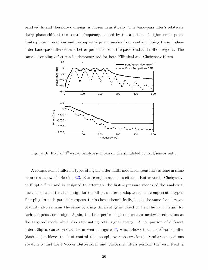
bandwidth, and therefore damping, is chosen heuristically. The band-pass filter’s relatively

sharp phase shift at the control frequency, caused by the addition of higher order poles,

limits phase interaction and decouples adjacent modes from control. Using these higher-

order band-pass filters ensure better performance in the pass-band and roll-off regions. The

same decoupling effect can be demonstrated for both Elliptical and Chebyshev filters.

0 100 200 300 400 500−80

−60

−40

−20

0

20

Mag

nitu

de (

dB)

Band−pass Fitler (BPF)Cont−Perf path w/ BPF

0 100 200 300 400 500−2000

−1500

−1000

−500

0

500

Pha

se (

deg)

Frequency (Hz)

Figure 16: FRF of 4th-order band-pass filters on the simulated control/sensor path.

A comparison of different types of higher-order multi-modal compensators is done in same

manner as shown in Section 3.3. Each compensator uses either a Butterworth, Chebyshev,

or Elliptic filter and is designed to attenuate the first 4 pressure modes of the analytical

duct. The same iterative design for the all-pass filter is adopted for all compensator types.

Damping for each parallel compensator is chosen heuristically, but is the same for all cases.

Stability also remains the same by using different gains based on half the gain margin for

each compensator design. Again, the best performing compensator achieves reductions at

the targeted mode while also attenuating total signal energy. A comparison of different

order Elliptic controllers can be in seen in Figure 17, which shows that the 6th-order filter

(dash-dot) achieves the best control (due to spill-over observations). Similar comparisons

are done to find the 4th-order Butterworth and Chebyshev filters perform the best. Next, a

26

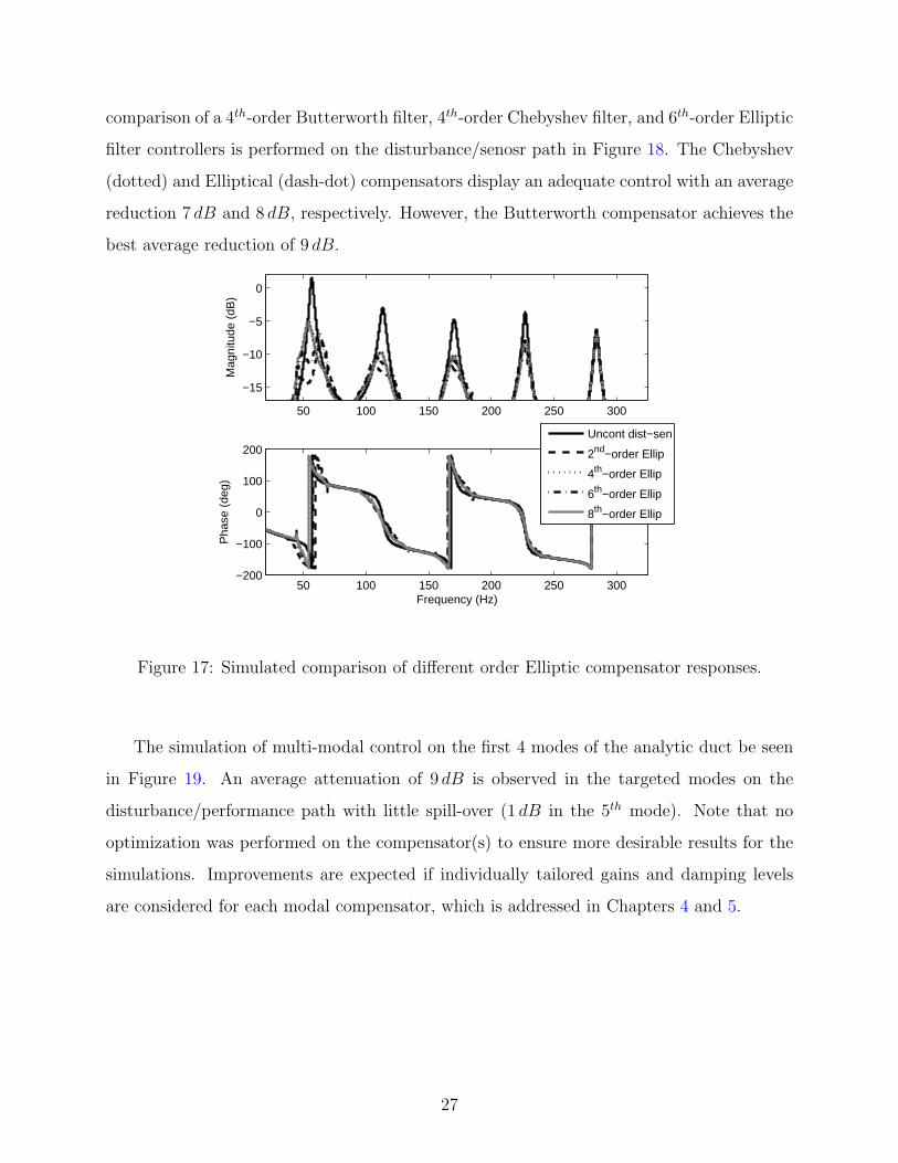
comparison of a 4th-order Butterworth filter, 4th-order Chebyshev filter, and 6th-order Elliptic

filter controllers is performed on the disturbance/senosr path in Figure 18. The Chebyshev

(dotted) and Elliptical (dash-dot) compensators display an adequate control with an average

reduction 7 dB and 8 dB, respectively. However, the Butterworth compensator achieves the

best average reduction of 9 dB.

50 100 150 200 250 300

−15

−10

−5

0

Mag

nitu

de (

dB)

50 100 150 200 250 300−200

−100

0

100

200

Pha

se (

deg)

Frequency (Hz)

Uncont dist−sen

2nd−order Ellip

4th−order Ellip

6th−order Ellip

8th−order Ellip

Figure 17: Simulated comparison of different order Elliptic compensator responses.

The simulation of multi-modal control on the first 4 modes of the analytic duct be seen

in Figure 19. An average attenuation of 9 dB is observed in the targeted modes on the

disturbance/performance path with little spill-over (1 dB in the 5th mode). Note that no

optimization was performed on the compensator(s) to ensure more desirable results for the

simulations. Improvements are expected if individually tailored gains and damping levels

are considered for each modal compensator, which is addressed in Chapters 4 and 5.

27

50 100 150 200 250 300

−15

−10

−5

0

Mag

nitu

de (

dB)

50 100 150 200 250 300−200

−100

0

100

200

Pha

se (

deg)

Frequency (Hz)

Uncont dist−sen

4th−order Butter

4th−order Cheby

6th−order Ellip

Figure 18: Simulated comparison of multi-modal Butterworth, Chebyshev, and Ellipitical

controller responses.

0 100 200 300 400 500−50

−40

−30

−20

−10

0

Mag

nitu

de (

dB)

0 100 200 300 400 500−200

−100

0

100

200

Pha

se (

deg)

Frequency (Hz)

Uncont dist−perfCont dist−perf

Figure 19: FRF of simulated disturbance/performance path showing 4-mode control.

28

4.0 EXPERIMENTAL DEMONSTRATION

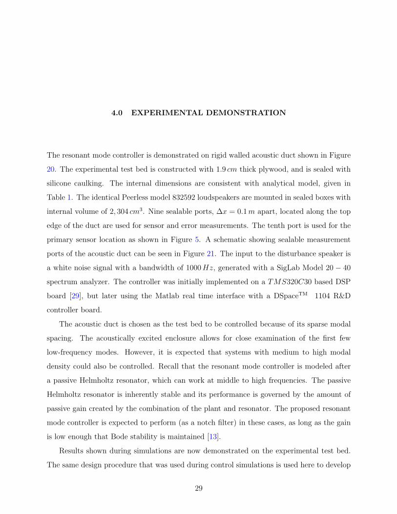
The resonant mode controller is demonstrated on rigid walled acoustic duct shown in Figure

20. The experimental test bed is constructed with 1.9 cm thick plywood, and is sealed with

silicone caulking. The internal dimensions are consistent with analytical model, given in

Table 1. The identical Peerless model 832592 loudspeakers are mounted in sealed boxes with

internal volume of 2, 304 cm3. Nine sealable ports, ∆x = 0.1m apart, located along the top

edge of the duct are used for sensor and error measurements. The tenth port is used for the

primary sensor location as shown in Figure 5. A schematic showing sealable measurement

ports of the acoustic duct can be seen in Figure 21. The input to the disturbance speaker is

a white noise signal with a bandwidth of 1000Hz, generated with a SigLab Model 20 − 40

spectrum analyzer. The controller was initially implemented on a TMS320C30 based DSP

board [29], but later using the Matlab real time interface with a DSpaceTM 1104 R&D

controller board.

The acoustic duct is chosen as the test bed to be controlled because of its sparse modal

spacing. The acoustically excited enclosure allows for close examination of the first few

low-frequency modes. However, it is expected that systems with medium to high modal

density could also be controlled. Recall that the resonant mode controller is modeled after

a passive Helmholtz resonator, which can work at middle to high frequencies. The passive

Helmholtz resonator is inherently stable and its performance is governed by the amount of

passive gain created by the combination of the plant and resonator. The proposed resonant

mode controller is expected to perform (as a notch filter) in these cases, as long as the gain

is low enough that Bode stability is maintained [13].

Results shown during simulations are now demonstrated on the experimental test bed.

The same design procedure that was used during control simulations is used here to develop

29

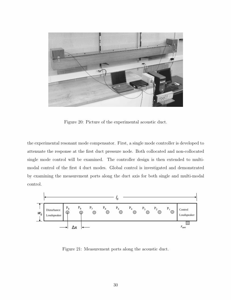
Figure 20: Picture of the experimental acoustic duct.

the experimental resonant mode compensator. First, a single mode controller is developed to

attenuate the response at the first duct pressure node. Both collocated and non-collocated

single mode control will be examined. The controller design is then extended to multi-

modal control of the first 4 duct modes. Global control is investigated and demonstrated

by examining the measurement ports along the duct axis for both single and multi-modal

control.

wdDisturbance

Loudspeaker

Control

Loudspeaker

P9 P8 P7 P6 P5 P4 P3 P2 P1

∆x

ld

xsen

Figure 21: Measurement ports along the acoustic duct.

30

4.1 SINGLE MODE CONTROL

The resonant mode controller is now demonstrated on the experimental test bed to control

the first acoustic mode. The same design procedure that was used to develop the single

mode controller during simulation is used here. The two-port diagram shown in Figure 7

used to define the transfer function paths during simulations is used to describe the transfer

function paths of the experimental duct. The uncontrolled control/sensor path, Hcs(s), is

examined to determine the phase at the control frequency. Next, a Butterworth band-pass

filter is added to Hcs(s), tuned to the desired mode of control. A phase-compensating all-

pass filter is then added to the controller to ensure that a 180o phase shift occurs at ωc. The

effectiveness of the controller is evaluated on the disturbance paths, Hds(s) and Hdp(s). It

was shown during control simulations in Chapter 3 that any single mode can be controlled,

which is also the case here. Also, the Nyquist stability analysis that was illustrated during

single mode simulation is applied here in the experimental demonstration.

All ANC systems use a loudspeaker as an actuator to drive a control signal. The con-

trol speaker effectively adds energy to the system, which could conceivably be preventing

the disturbance speaker from actuating (i.e. source-loading). However, unlike feedforward

methods where energy densities and an a priori reference signal must be considered [26],

feedback control can augment the system parameters to ensure that the disturbance speaker

is uninhibited. By measuring the surface acceleration and power input to the disturbance

speaker, which remained unchanged for both uncontrolled and controlled cases, a non-source

loaded compensator was confirmed. This was achieved using a model U352C22 accelerom-

eter by PCB Piezotronics and a post processing integrator circuit. The results comparing

disturbance speaker power, acceleration, and velocity for uncontrolled and controlled cases

can be seen in Table 2.

Reducing the noise at a specific location often has the unwanted side effect of increasing

noise elsewhere. However, the rigid-walled duct creates a simple sound field that makes

global reduction possible. Unlike other works [16, 27], the performance sensor can be moved

along the 10 equally space ports along the duct axis, shown in Figure 21, to evaluate whether

or not global control is achieved. Two types of control will be considered for single mode

31

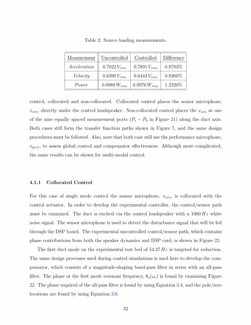
Table 2: Source loading measurements.

Measurement Uncontrolled Controlled Difference

Acceleration 0.7822Vrms 0.7891Vrms 0.8783%

Velocity 0.6390Vrms 0.6443Vrms 0.8260%

Power 0.0988Wrms 0.0976Wrms 1.2220%

control, collocated and non-collocated. Collocated control places the sensor microphone,

xsen, directly under the control loudspeaker. Non-collocated control places the xsen at one

of the nine equally spaced measurement ports (P1 − P9 in Figure 21) along the duct axis.

Both cases still form the transfer function paths shown in Figure 7, and the same design

procedures must be followed. Also, note that both case still use the performance microphone,

xperf , to assess global control and compensator effectiveness. Although more complicated,

the same results can be shown for multi-modal control.

4.1.1 Collocated Control

For this case of single mode control the sensor microphone, xsen, is collocated with the

control actuator. In order to develop the experimental controller, the control/sensor path

must be examined. The duct is excited via the control loudspeaker with a 1000Hz white

noise signal. The sensor microphone is used to detect the disturbance signal that will be fed

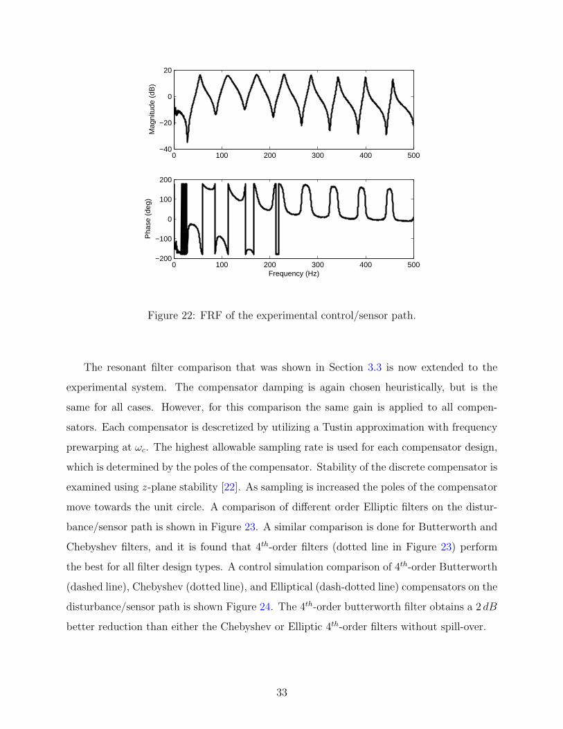
through the DSP board. The experimental uncontrolled control/sensor path, which contains

phase contributions from both the speaker dynamics and DSP card, is shown in Figure 22.

The first duct mode on the experimental test bed of 54.37Hz is targeted for reduction.

The same design processes used during control simulations is used here to develop the com-

pensator, which consists of a magnitude-shaping band-pass filter in series with an all-pass

filter. The phase at the first mode resonant frequency, θa(ωc) is found by examining Figure

22. The phase required of the all-pass filter is found by using Equation 3.4, and the pole/zero

locations are found by using Equation 3.6.

32

0 100 200 300 400 500−40

−20

0

20

Mag

nitu

de (

dB)

0 100 200 300 400 500−200

−100

0

100

200

Frequency (Hz)

Pha

se (

deg)

Figure 22: FRF of the experimental control/sensor path.

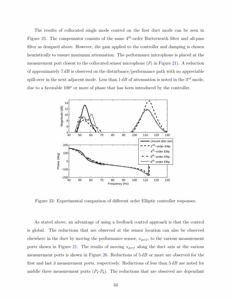
The resonant filter comparison that was shown in Section 3.3 is now extended to the

experimental system. The compensator damping is again chosen heuristically, but is the

same for all cases. However, for this comparison the same gain is applied to all compen-

sators. Each compensator is descretized by utilizing a Tustin approximation with frequency

prewarping at ωc. The highest allowable sampling rate is used for each compensator design,

which is determined by the poles of the compensator. Stability of the discrete compensator is

examined using z -plane stability [22]. As sampling is increased the poles of the compensator

move towards the unit circle. A comparison of different order Elliptic filters on the distur-

bance/sensor path is shown in Figure 23. A similar comparison is done for Butterworth and

Chebyshev filters, and it is found that 4th-order filters (dotted line in Figure 23) perform

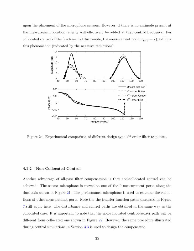
the best for all filter design types. A control simulation comparison of 4th-order Butterworth

(dashed line), Chebyshev (dotted line), and Elliptical (dash-dotted line) compensators on the

disturbance/sensor path is shown Figure 24. The 4th-order butterworth filter obtains a 2 dB

better reduction than either the Chebyshev or Elliptic 4th-order filters without spill-over.

33

The results of collocated single mode control on the first duct mode can be seen in

Figure 25. The compensator consists of the same 4th-order Butterworth filter and all-pass

filter as designed above. However, the gain applied to the controller and damping is chosen

heuristically to ensure maximum attenuation. The performance microphone is placed at the

measurement port closest to the collocated sensor microphone (P1 in Figure 21). A reduction

of approximately 7 dB is observed on the disturbance/performance path with no appreciable

spill-over in the next adjacent mode. Less than 1 dB of attenuation is noted in the 3rd mode,

due to a favorable 100o or more of phase that has been introduced by the controller.

40 50 60 70 80 90 100 110 120 1304

6

8

10

12

14

Mag

nitu

de (

dB)

40 50 60 70 80 90 100 110 120 130−200

−100

0

100

200

Pha

se (

deg)

Frequency (Hz)

Uncont dist−sen

2nd−order Ellip

4th−order Ellip

6th−order Ellip

8th−order Ellip

Figure 23: Experimental comparison of different order Elliptic controller responses.

As stated above, an advantage of using a feedback control approach is that the control

is global. The reductions that are observed at the sensor location can also be observed

elsewhere in the duct by moving the performance sensor, xperf , to the various measurement

ports shown in Figure 21. The results of moving xperf along the duct axis at the various

measurement ports is shown in Figure 26. Reductions of 5 dB or more are observed for the

first and last 3 measurement ports, respectively. Reductions of less than 5 dB are noted for

middle three measurement ports (P4-P6). The reductions that are observed are dependant

34

upon the placement of the microphone sensors. However, if there is no antinode present at

the measurement location, energy will effectively be added at that control frequency. For

collocated control of the fundamental duct mode, the measurement point xperf = P5 exhibits

this phenomenon (indicated by the negative reductions).

40 50 60 70 80 90 100 110 120 1304

6

8

10

12

14M

agni

tude

(dB

)

40 50 60 70 80 90 100 110 120 130−200

−100

0

100

200

Pha

se (

deg)

Frequency (Hz)

Uncont dist−sen

4th−order Butter

4th−order Cheby

4th−order Ellip

Figure 24: Experimental comparison of different design-type 4th-order filter responses.

4.1.2 Non-Collocated Control

Another advantage of all-pass filter compensation is that non-collocated control can be

achieved. The sensor microphone is moved to one of the 9 measurement ports along the

duct axis shown in Figure 21. The performance microphone is used to examine the reduc-

tions at other measurement ports. Note the the transfer function paths discussed in Figure

7 still apply here. The disturbance and control paths are obtained in the same way as the

collocated case. It is important to note that the non-collocated control/sensor path will be

different from collocated one shown in Figure 22. However, the same procedure illustrated

during control simulations in Section 3.3 is used to design the compensator.

35

40 60 80 100 120 140 160 1800

5

10

15

Mag

nitu

de (

dB)

Frequency (Hz)

Uncont dist−perfControl dist−perf

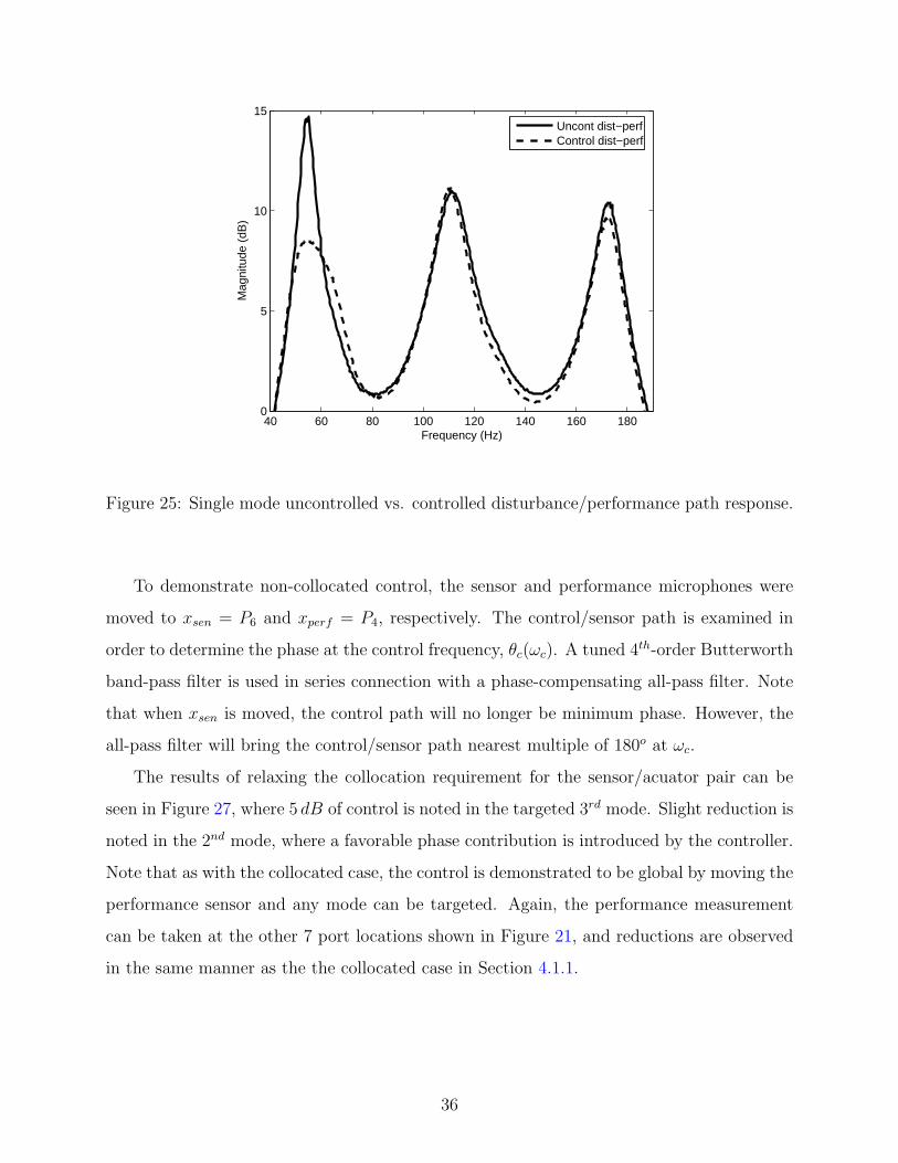
Figure 25: Single mode uncontrolled vs. controlled disturbance/performance path response.

To demonstrate non-collocated control, the sensor and performance microphones were

moved to xsen = P6 and xperf = P4, respectively. The control/sensor path is examined in

order to determine the phase at the control frequency, θc(ωc). A tuned 4th-order Butterworth

band-pass filter is used in series connection with a phase-compensating all-pass filter. Note

that when xsen is moved, the control path will no longer be minimum phase. However, the

all-pass filter will bring the control/sensor path nearest multiple of 180o at ωc.

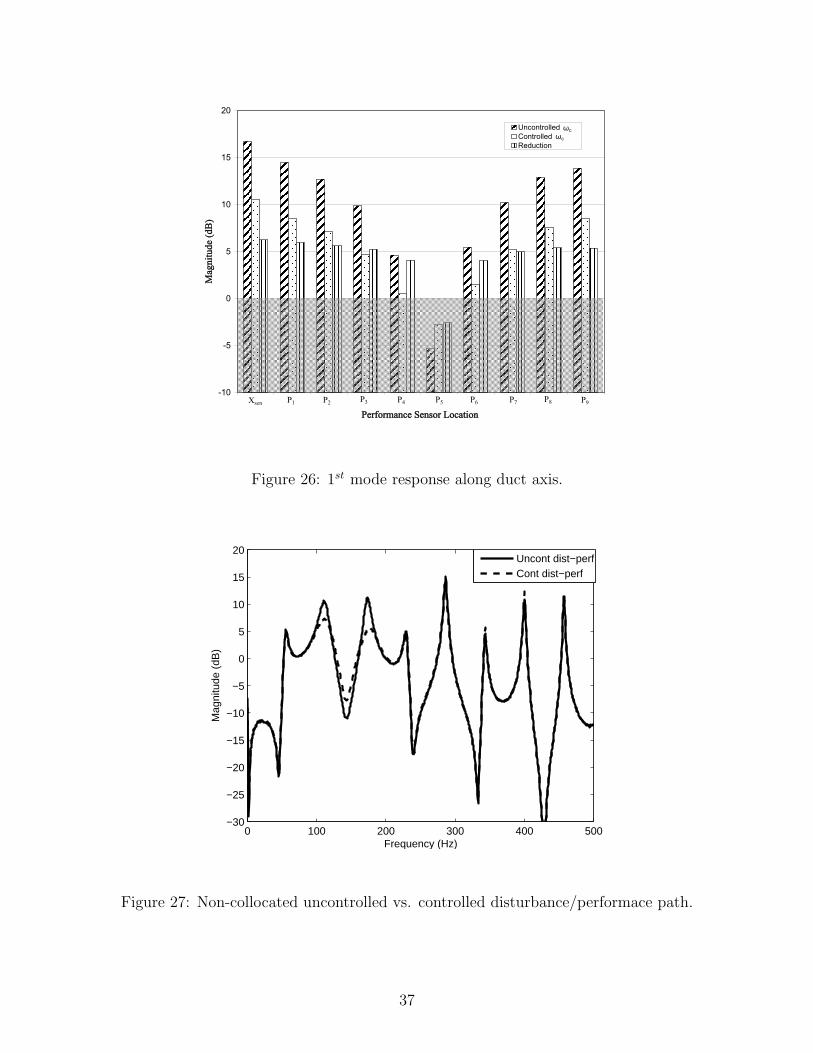
The results of relaxing the collocation requirement for the sensor/acuator pair can be

seen in Figure 27, where 5 dB of control is noted in the targeted 3rd mode. Slight reduction is

noted in the 2nd mode, where a favorable phase contribution is introduced by the controller.

Note that as with the collocated case, the control is demonstrated to be global by moving the

performance sensor and any mode can be targeted. Again, the performance measurement

can be taken at the other 7 port locations shown in Figure 21, and reductions are observed

in the same manner as the the collocated case in Section 4.1.1.

36

-10

-5

0

5

10

15

20

xsen P1 P2 P3 P4 P5 P6 P7 P8 P9

Performance Sensor Location

Mag

nitu

de (d

B)

Uncontrolled Controlled Reduction

Xsen P1 P2 P3 P4 P5 P6 P7 P8 P9

ωcωc

Figure 26: 1st mode response along duct axis.

0 100 200 300 400 500−30

−25

−20

−15

−10

−5

0

5

10

15

20

Frequency (Hz)

Mag

nitu

de (

dB)

Uncont dist−perfCont dist−perf

Figure 27: Non-collocated uncontrolled vs. controlled disturbance/performace path.

37

4.2 MULTIPLE MODE CONTROL

The procedure for controlling a single acoustic mode is now extended to multiple modes.

Returning to Figure 22, the first 4 pressure modes are targeted for control shown in Table 3.

Note that the acoustic loudspeaker and sensor microphone are collocated as shown by the

control path response in Figure 22. The compensator is realized in the same manner as the

single mode case. Each mode controller, which consists of a compensating filter and phase

correction filter, is connected in parallel to form the multi-modal controller.

Table 3: First 4 pressure nodes of the acoustic duct.

Mode Number Frequency

1 54.37Hz

2 111.56Hz

3 172.5Hz

4 228.75Hz

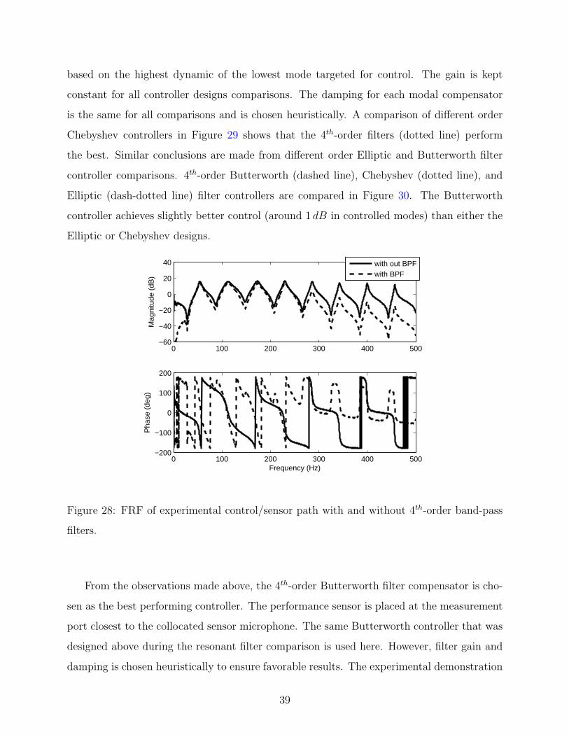
A key difference in the design approach is that the magnitude shaping band-pass filters

must be added to the control/sensor path before the all-pass filters are designed. The

experimental control/sensor path with (dashed line) and without (solid line) the 4th order

Butterworth band-pass filters are shown in Figure 28. The butterworth filter damping was

determined in the manner shown during multi-modal control simulations. The phase required

of the all-pass filter is determined from the dashed line in Figure 28 by examining the phase

at the control frequencies. Figure 28 also shows the decoupling effect of the band-pass filters.

The all-pass filters are implemented at each mode to achieve the desired 180o of phase at each

mode. Again, the same stability analysis that was performed on the single mode controller

during control simulations is administered here.

The resonant filter comparison that was done for the experimental single mode controller

is now extended to the multi-modal controller. The same discretization process that was used

for the single mode controller comparison is used here. The highest sampling rate is chosen

38

based on the highest dynamic of the lowest mode targeted for control. The gain is kept

constant for all controller designs comparisons. The damping for each modal compensator

is the same for all comparisons and is chosen heuristically. A comparison of different order

Chebyshev controllers in Figure 29 shows that the 4th-order filters (dotted line) perform

the best. Similar conclusions are made from different order Elliptic and Butterworth filter

controller comparisons. 4th-order Butterworth (dashed line), Chebyshev (dotted line), and

Elliptic (dash-dotted line) filter controllers are compared in Figure 30. The Butterworth

controller achieves slightly better control (around 1 dB in controlled modes) than either the

Elliptic or Chebyshev designs.

0 100 200 300 400 500−60

−40

−20

0

20

40

Mag

nitu

de (

dB)

with out BPFwith BPF

0 100 200 300 400 500−200

−100

0

100

200

Pha

se (

deg)

Frequency (Hz)

Figure 28: FRF of experimental control/sensor path with and without 4th-order band-pass

filters.

From the observations made above, the 4th-order Butterworth filter compensator is cho-

sen as the best performing controller. The performance sensor is placed at the measurement

port closest to the collocated sensor microphone. The same Butterworth controller that was

designed above during the resonant filter comparison is used here. However, filter gain and

damping is chosen heuristically to ensure favorable results. The experimental demonstration

39

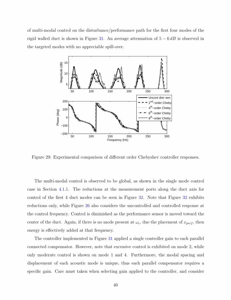
of multi-modal control on the disturbance/performance path for the first four modes of the

rigid walled duct is shown in Figure 31. An average attenuation of 5 − 6 dB is observed in

the targeted modes with no appreciable spill-over.

50 100 150 200 250 300

5

10

15M

agni

tude

(dB

)

50 100 150 200 250 300−200

−100

0

100

200

Pha

se (

deg)

Frequency (Hz)

Uncont dist−sen

2nd−order Cheby

4th−order Cheby

6th−order Cheby

8th−order Cheby

Figure 29: Experimental comparison of different order Chebyshev controller responses.

The multi-modal control is observed to be global, as shown in the single mode control

case in Section 4.1.1. The reductions at the measurement ports along the duct axis for

control of the first 4 duct modes can be seen in Figure 32. Note that Figure 32 exhibits

reductions only, while Figure 26 also considers the uncontrolled and controlled response at

the control frequency. Control is diminished as the performance sensor is moved toward the

center of the duct. Again, if there is no mode present at ωc, due the placement of xperf , then

energy is effectively added at that frequency.

The controller implemented in Figure 31 applied a single controller gain to each parallel

connected compensator. However, note that excessive control is exhibited on mode 2, while

only moderate control is shown on mode 1 and 4. Furthermore, the modal spacing and

displacement of each acoustic mode is unique, thus each parallel compensator requires a

specific gain. Care must taken when selecting gain applied to the controller, and consider

40

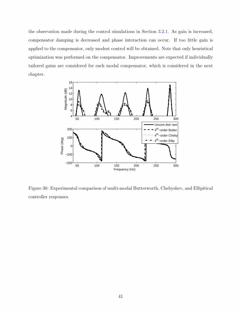
the observation made during the control simulations in Section 3.2.1. As gain is increased,

compensator damping is decreased and phase interaction can occur. If too little gain is

applied to the compensator, only modest control will be obtained. Note that only heuristical

optimization was performed on the compensator. Improvements are expected if individually

tailored gains are considered for each modal compensator, which is considered in the next

chapter.

50 100 150 200 250 3004

6

8

10

12

14

16

Mag

nitu

de (

dB)

50 100 150 200 250 300−200

−100

0

100

200

Pha

se (

deg)

Frequency (Hz)

Uncont dist−sen

4th−order Butter

4th−order Cheby

4th−order Ellip

Figure 30: Experimental comparison of multi-modal Butterworth, Chebyshev, and Ellipitical

controller responses.

41

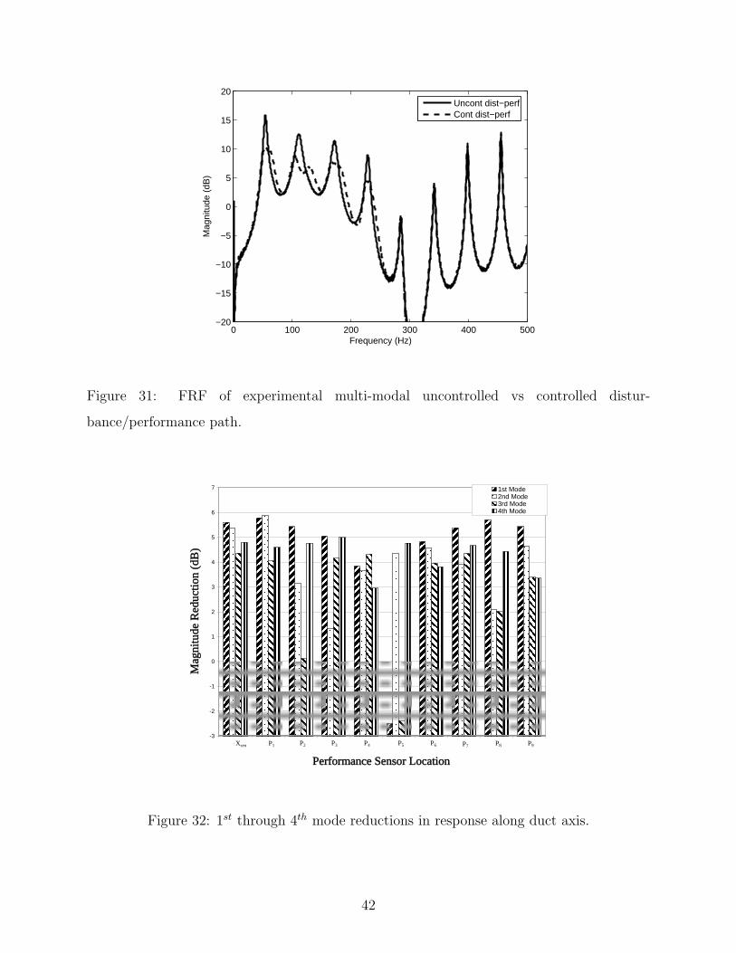
0 100 200 300 400 500−20

−15

−10

−5

0

5

10

15

20

Mag

nitu

de (

dB)

Frequency (Hz)

Uncont dist−perfCont dist−perf

Figure 31: FRF of experimental multi-modal uncontrolled vs controlled distur-

bance/performance path.

-3

-2

-1

0

1

2

3

4

5

6

7

s 1 2 3 4 5 6 7 8 9

Performance Sensor Location

Mag

nitu

de R

educ

tion

(dB

)

1st Mode2nd Mode3rd Mode4th Mode

P6P5P4P3Xsen P1 P2 P7 P8 P9

Figure 32: 1st through 4th mode reductions in response along duct axis.

42

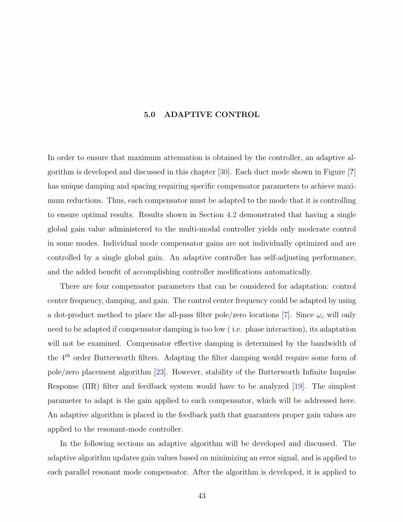
5.0 ADAPTIVE CONTROL

In order to ensure that maximum attenuation is obtained by the controller, an adaptive al-

gorithm is developed and discussed in this chapter [30]. Each duct mode shown in Figure [?]

has unique damping and spacing requiring specific compensator parameters to achieve maxi-

mum reductions. Thus, each compensator must be adapted to the mode that it is controlling

to ensure optimal results. Results shown in Section 4.2 demonstrated that having a single

global gain value administered to the multi-modal controller yields only moderate control

in some modes. Individual mode compensator gains are not individually optimized and are

controlled by a single global gain. An adaptive controller has self-adjusting performance,

and the added benefit of accomplishing controller modifications automatically.

There are four compensator parameters that can be considered for adaptation: control

center frequency, damping, and gain. The control center frequency could be adapted by using

a dot-product method to place the all-pass filter pole/zero locations [7]. Since ωc will only

need to be adapted if compensator damping is too low ( i.e. phase interaction), its adaptation

will not be examined. Compensator effective damping is determined by the bandwidth of

the 4th order Butterworth filters. Adapting the filter damping would require some form of

pole/zero placement algorithm [23]. However, stability of the Butterworth Infinite Impulse

Response (IIR) filter and feedback system would have to be analyzed [19]. The simplest

parameter to adapt is the gain applied to each compensator, which will be addressed here.

An adaptive algorithm is placed in the feedback path that guarantees proper gain values are

applied to the resonant-mode controller.

In the following sections an adaptive algorithm will be developed and discussed. The

adaptive algorithm updates gain values based on minimizing an error signal, and is applied to

each parallel resonant mode compensator. After the algorithm is developed, it is applied to

43

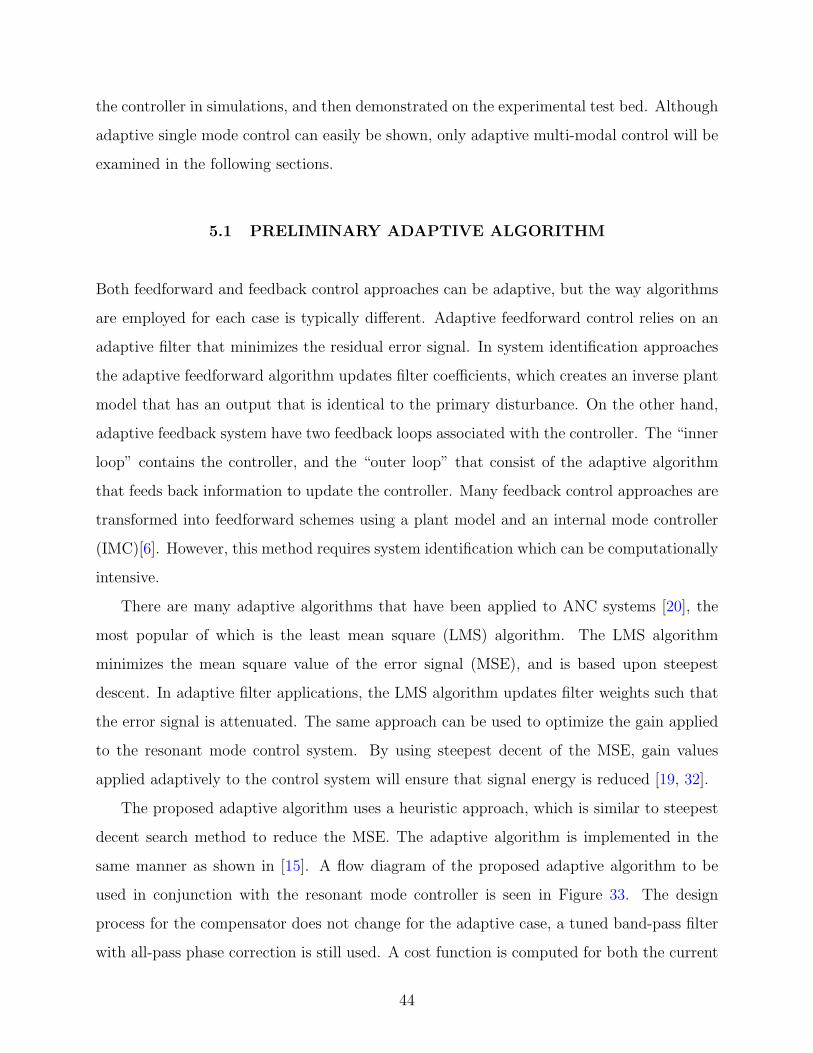
the controller in simulations, and then demonstrated on the experimental test bed. Although

adaptive single mode control can easily be shown, only adaptive multi-modal control will be

examined in the following sections.

5.1 PRELIMINARY ADAPTIVE ALGORITHM

Both feedforward and feedback control approaches can be adaptive, but the way algorithms

are employed for each case is typically different. Adaptive feedforward control relies on an

adaptive filter that minimizes the residual error signal. In system identification approaches

the adaptive feedforward algorithm updates filter coefficients, which creates an inverse plant

model that has an output that is identical to the primary disturbance. On the other hand,

adaptive feedback system have two feedback loops associated with the controller. The “inner

loop” contains the controller, and the “outer loop” that consist of the adaptive algorithm

that feeds back information to update the controller. Many feedback control approaches are

transformed into feedforward schemes using a plant model and an internal mode controller

(IMC)[6]. However, this method requires system identification which can be computationally

intensive.

There are many adaptive algorithms that have been applied to ANC systems [20], the

most popular of which is the least mean square (LMS) algorithm. The LMS algorithm

minimizes the mean square value of the error signal (MSE), and is based upon steepest

descent. In adaptive filter applications, the LMS algorithm updates filter weights such that

the error signal is attenuated. The same approach can be used to optimize the gain applied

to the resonant mode control system. By using steepest decent of the MSE, gain values

applied adaptively to the control system will ensure that signal energy is reduced [19, 32].

The proposed adaptive algorithm uses a heuristic approach, which is similar to steepest

decent search method to reduce the MSE. The adaptive algorithm is implemented in the

same manner as shown in [15]. A flow diagram of the proposed adaptive algorithm to be

used in conjunction with the resonant mode controller is seen in Figure 33. The design

process for the compensator does not change for the adaptive case, a tuned band-pass filter

with all-pass phase correction is still used. A cost function is computed for both the current

44

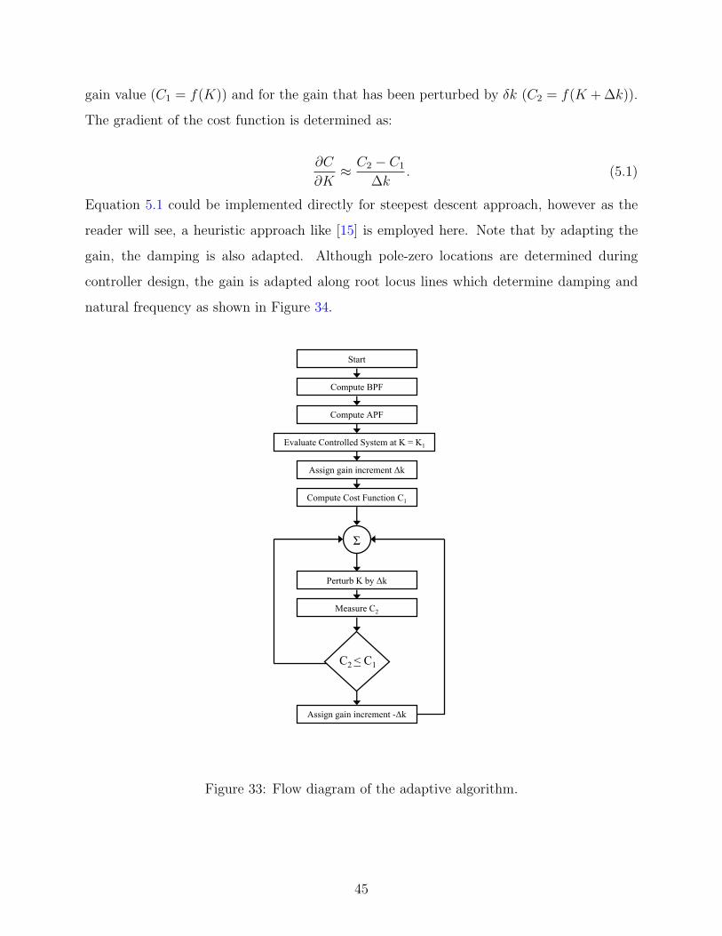
gain value (C1 = f(K)) and for the gain that has been perturbed by δk (C2 = f(K + ∆k)).

The gradient of the cost function is determined as:

∂C

∂K≈ C2 − C1

∆k. (5.1)

Equation 5.1 could be implemented directly for steepest descent approach, however as the

reader will see, a heuristic approach like [15] is employed here. Note that by adapting the

gain, the damping is also adapted. Although pole-zero locations are determined during

controller design, the gain is adapted along root locus lines which determine damping and

natural frequency as shown in Figure 34.

Start

Compute BPF

Compute APF

Evaluate Controlled System at K = K1

Assign gain increment ∆k

Compute Cost Function C1

Σ

Measure C2

Perturb K by ∆k

Assign gain increment -∆k

C2 < C1

Figure 33: Flow diagram of the adaptive algorithm.

45

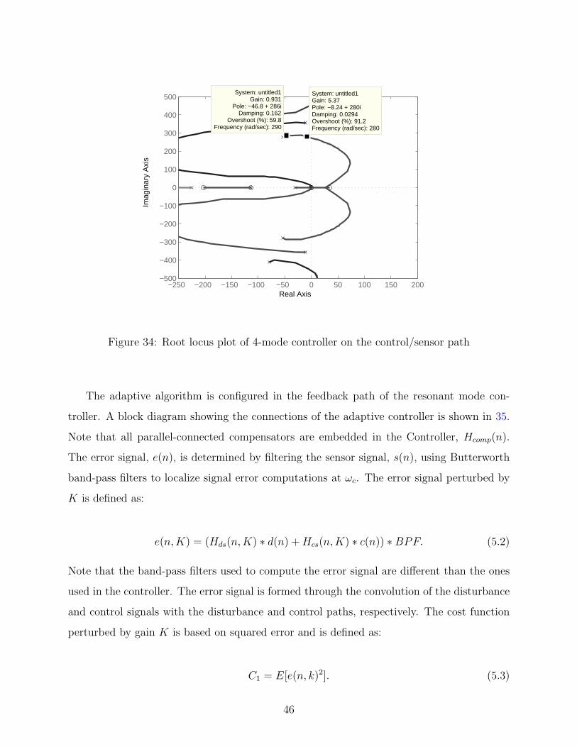
Real Axis

Imag

inar

y A

xis

−250 −200 −150 −100 −50 0 50 100 150 200−500

−400

−300

−200

−100

0

100

200

300

400

500System: untitled1

Gain: 0.931Pole: −46.8 + 286i

Damping: 0.162Overshoot (%): 59.8

Frequency (rad/sec): 290

System: untitled1Gain: 5.37Pole: −8.24 + 280iDamping: 0.0294Overshoot (%): 91.2Frequency (rad/sec): 280

Figure 34: Root locus plot of 4-mode controller on the control/sensor path

The adaptive algorithm is configured in the feedback path of the resonant mode con-

troller. A block diagram showing the connections of the adaptive controller is shown in 35.

Note that all parallel-connected compensators are embedded in the Controller, Hcomp(n).

The error signal, e(n), is determined by filtering the sensor signal, s(n), using Butterworth

band-pass filters to localize signal error computations at ωc. The error signal perturbed by

K is defined as:

e(n,K) = (Hds(n,K) ∗ d(n) +Hcs(n,K) ∗ c(n)) ∗BPF. (5.2)

Note that the band-pass filters used to compute the error signal are different than the ones

used in the controller. The error signal is formed through the convolution of the disturbance

and control signals with the disturbance and control paths, respectively. The cost function

perturbed by gain K is based on squared error and is defined as:

C1 = E[e(n, k)2]. (5.3)

46

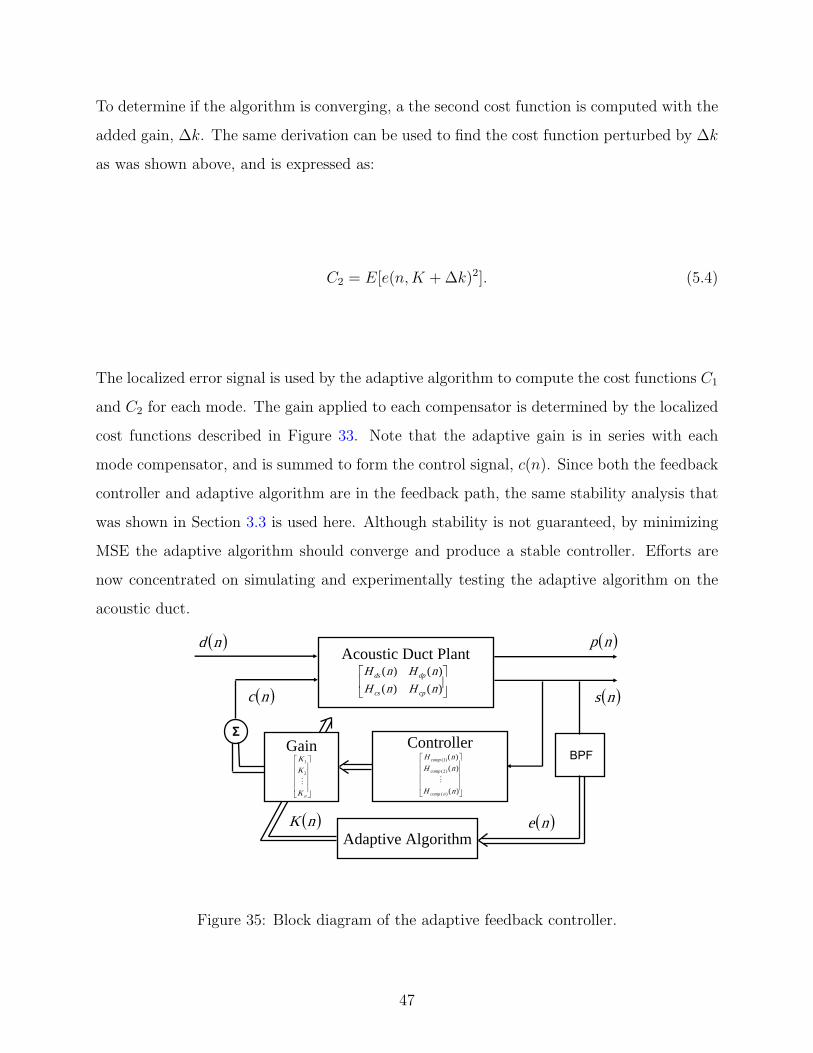
To determine if the algorithm is converging, a the second cost function is computed with the

added gain, ∆k. The same derivation can be used to find the cost function perturbed by ∆k

as was shown above, and is expressed as:

C2 = E[e(n,K + ∆k)2]. (5.4)

The localized error signal is used by the adaptive algorithm to compute the cost functions C1

and C2 for each mode. The gain applied to each compensator is determined by the localized

cost functions described in Figure 33. Note that the adaptive gain is in series with each

mode compensator, and is summed to form the control signal, c(n). Since both the feedback

controller and adaptive algorithm are in the feedback path, the same stability analysis that

was shown in Section 3.3 is used here. Although stability is not guaranteed, by minimizing

MSE the adaptive algorithm should converge and produce a stable controller. Efforts are

now concentrated on simulating and experimentally testing the adaptive algorithm on the

acoustic duct.

Acoustic Duct Plant

Controller

Adaptive Algorithm

Gain

( )ne( )nK

( )nd

( )nc ( )ns

BPF

( )np

⎥⎦

⎤⎢⎣

⎡)()()()(

nHnHnHnH

cpcs

dpds

⎥⎥⎥⎥

⎦

⎤

⎢⎢⎢⎢

⎣

⎡

)(

)()(

)(

)2(

)1(

nH

nHnH

ncomp

comp

comp

M⎥⎥⎥⎥

⎦

⎤

⎢⎢⎢⎢

⎣

⎡

nK

KK

M2

1

Σ

Figure 35: Block diagram of the adaptive feedback controller.

47

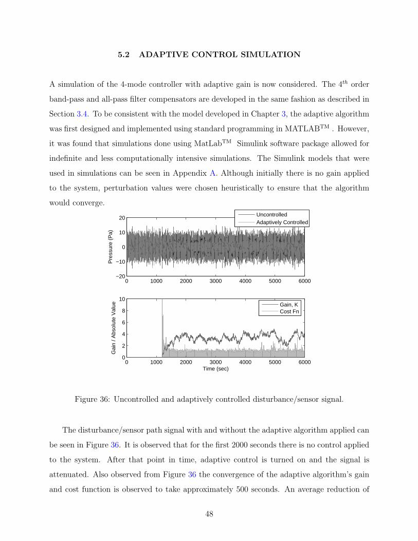
5.2 ADAPTIVE CONTROL SIMULATION

A simulation of the 4-mode controller with adaptive gain is now considered. The 4th order

band-pass and all-pass filter compensators are developed in the same fashion as described in

Section 3.4. To be consistent with the model developed in Chapter 3, the adaptive algorithm

was first designed and implemented using standard programming in MATLABTM . However,

it was found that simulations done using MatLabTM Simulink software package allowed for

indefinite and less computationally intensive simulations. The Simulink models that were

used in simulations can be seen in Appendix A. Although initially there is no gain applied

to the system, perturbation values were chosen heuristically to ensure that the algorithm

would converge.

0 1000 2000 3000 4000 5000 6000−20

−10

0

10

20

Pre

ssur

e (P

a)

0 1000 2000 3000 4000 5000 60000

2

4

6

8

10

Time (sec)

Gai

n / A

bsol

ute

Val

ue

UncontrolledAdaptively Controlled

Gain, KCost Fn

Figure 36: Uncontrolled and adaptively controlled disturbance/sensor signal.

The disturbance/sensor path signal with and without the adaptive algorithm applied can

be seen in Figure 36. It is observed that for the first 2000 seconds there is no control applied

to the system. After that point in time, adaptive control is turned on and the signal is

attenuated. Also observed from Figure 36 the convergence of the adaptive algorithm’s gain

and cost function is observed to take approximately 500 seconds. An average reduction of

48

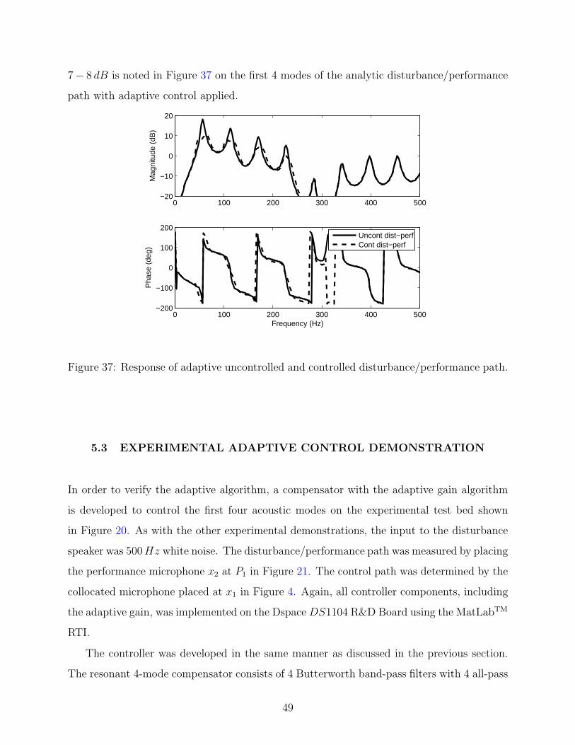
7− 8 dB is noted in Figure 37 on the first 4 modes of the analytic disturbance/performance

path with adaptive control applied.

0 100 200 300 400 500−20

−10

0

10

20

Mag

nitu

de (

dB)

0 100 200 300 400 500−200

−100

0

100

200

Pha

se (

deg)

Frequency (Hz)

Uncont dist−perfCont dist−perf

Figure 37: Response of adaptive uncontrolled and controlled disturbance/performance path.

5.3 EXPERIMENTAL ADAPTIVE CONTROL DEMONSTRATION

In order to verify the adaptive algorithm, a compensator with the adaptive gain algorithm

is developed to control the first four acoustic modes on the experimental test bed shown

in Figure 20. As with the other experimental demonstrations, the input to the disturbance

speaker was 500Hz white noise. The disturbance/performance path was measured by placing

the performance microphone x2 at P1 in Figure 21. The control path was determined by the

collocated microphone placed at x1 in Figure 4. Again, all controller components, including

the adaptive gain, was implemented on the DspaceDS1104 R&D Board using the MatLabTM

RTI.

The controller was developed in the same manner as discussed in the previous section.

The resonant 4-mode compensator consists of 4 Butterworth band-pass filters with 4 all-pass

49

filters tuned at the target frequency of each mode. Filter damping is unique to each compen-

sator, and is chosen in a heuristic manner shown in chapters 3 and 4. The disturbance/sensor

path is processed by the DSP where the adaptive algorithm and controller are implemented

to create the control path. The recursive algorithm updates gain applied to each parallel

connected compensator so that the error signal energy is minimized. The Simulink Block

Diagrams that were used to implement the adaptive control can be seen in Appendix B.

The adaptive uncontrolled and controlled system response is plotted in Figure 38. A

balance between filter damping and gain is achieved by reducing the sensor signal error.

An average reduction of 6 − 7 dB has been observed in each of the controlled modes, with

improvements of 3 dB in the fist mode and 2 dB fourth mode. Unlike the non-adaptive

case, the adaptive resonant mode controller achieves maximum control at each mode. Since

the MSE signal is minimized by the algorithm and the gain for each mode is individually

tailored, this is the best possible reduction that can be obtained with the given filter damping

parameters. The adaptive algorithm also guarantees that the modes will not “split” from

excess gain [5], and create a worse modal response at shifted frequencies.

50

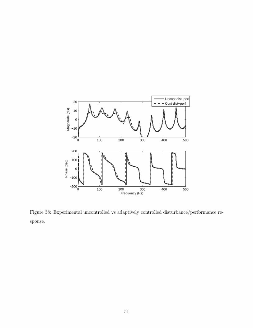
0 100 200 300 400 500−20

−10

0

10

20

Mag

nitu

de (

dB)

0 100 200 300 400 500−200

−100

0

100

200

Frequency (Hz)

Pha

se (

deg)

Uncont dist−perfCont dist−perf

Figure 38: Experimental uncontrolled vs adaptively controlled disturbance/performance re-

sponse.

51

6.0 CONCLUSIONS AND FUTURE WORK

Several refinements have been incorporated into a new type of acoustic control system that

uses positive position feedback (PPF) with damped, resonant filters [4]. Past studies have

concentrated on the design and component architecture of PPF applied to acoustic systems.

By examining design variables, insight has been gained into creating a more efficient resonant

mode controller. Realizing the controller using a digital signal processor (DSP) board allowed

for easy examination of the design parameters, and greatly facilitated control beyond two

modes. System refinements were first simulated using an analytical duct model, and then

demonstrated on the experimental test bed. Finally, a adaptive algorithm was developed

and implemented to update gain values applied to the multi-modal control filters.

The type of resonant filter used in the compensator has a profound impact system per-

formance for both single and multi-modal control. Band-Pass filters, rather than low-pass

filters, were found to give improved results when considering multi-modal control. Band-

pass filters provide magnitude roll-off at both high and low frequencies around ωc, while

also allowing for a sharper phase shift. This was found to help de-couple phase interac-

tions between controlled and uncontrolled modes. Three types of higher-order band-pass

filters were investigated: Butterworth, Chebyshev, and Elliptic. Through control system

simulations, it was found that 4th Butterworth filters provided roll-off of ±40 dB/dec and

maximally flat pass-band at the control frequency. Thus, Butterworth filters provide max-

imum attenuation, while also limiting phase interaction of controlled/uncontrolled modes.

The band-pass filters alone cannot achieve an “out of phase” signal and requires the use of

an all-pass phase-correction filter, as shown in previous studies [3]. The resonant controller

demonstrated reductions of 5 − 6 dB on the first four modes of the rigid-walled duct test

bed.

52

Placement of the microphone sensors determine the transfer function paths of the control

system. These system conventions were clarified to gain greater insight into performance

and stability of the controller. Since the resonant mode controller is a non-minimum phase

system, controller stability can not be guaranteed. However, Nyquist stability criterion was

used to evaluate the effects gain on controller performance and stability. The ability of the

phase compensation method to compensate a non-minimum phase system also allows for the

collocation requirement of standard PPF to be relaxed. Non-collocated was experimentally

demonstrated by moving the sensor microphone away from the control speaker, and 5 dB of

attenuation was noted.

Test were conducted to determine whether the type of control that being administered is

global or local. Global reduction was confirmed by utilizing a performance sensor with the 9

equally spaced duct measurement ports along the duct axis and comparing uncontrolled vs.

controlled responses. Attenuation is achieved at each measurement port, as long as their is a

pressure node present at the control frequency. Speaker power, acceleration, and velocity was

also measured for controlled and uncontrolled cases to ensure that the disturbance speaker

was unimpeded.

An adaptive algorithm is presented to ensure that proper gain levels are applied to

each mode of the controller. Each acoustic mode of the duct is unique, thus requiring

specific compensator gain and damping. The adaptive algorithm updates gain values based

on the mean square error (MSE) of the pressure signal that is fed back to the controller.

The adaptive controller assures that maximum reduction is obtained, given the damping

present in the compensator(s). An average adaptive control of 6 − 7 dB is observed on

the experimental test bed. The adaptive controller also has the added benefit of being self

adjusting, making it applicable to other closed cavity noise problems.

Compensator damping has the greatest impact on the performance of the resonant con-

trol system. Compensator damping is determined by the bandwidth of the Butterworth

band-pass filter [31, 22]. Although effects of the compensator damping was investigated

heuristically, some important observations were made. The amount of control and phase

interaction is proportional to the amount of compensator damping. Optimization of com-

pensator damping could be achieved in the same manner as tuned absorbers in structures.

53

However, parallels between acoustic (PPF) and mechanically tuned absorbers must first be

investigated.

Future work will further investigate the parameters and optimization of acoustic PPF.

The most important of these design parameters is the compensator damping and control

frequency. A compensator with adaptive damping and control frequency would achieve max-

imum reductions without causing phase shifts. The algorithm could use true steepest decent

to place the poles/zeros of the compensator. However, the theoretical limits of stability must

be examined in order to achieve a better defined control system. This would lead to easier

adaptation of other system parameters. In order to develop a better adaptive controller, the

stability of the adaptive feedback gain must be investigated. To better compare results, a

relationship between Helmholtz resonators, mechanically tuned absorbers, and acoustic PPF

using all-pass phase compensation must be defined. Realizing such a relationship would al-

low for optimization techniques already used for mechanically tuned absorbers [28]. Finally,

using a mix of filter types on different modes could lead to a better control system.

54

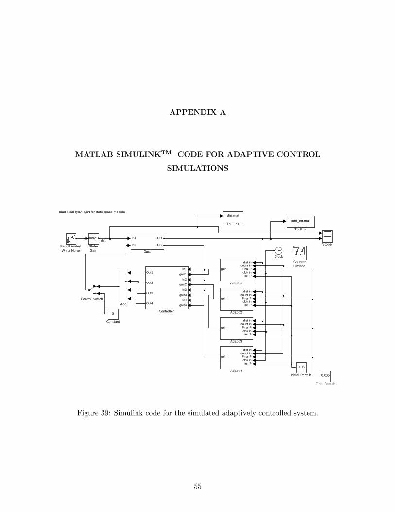
APPENDIX A

MATLAB SIMULINKTM CODE FOR ADAPTIVE CONTROL

SIMULATIONS

must load sysD, sysN for state space modelsdist.mat

To File1cont_err.mat

To File

.009216

SliderGain

Scope

0.05

Initial Pertrub 0.005

Final Perturb

In1

In2

Out1

Out2

Ductlim

CounterLimited

In1gain1

In2

gain2In3

gain3In4

gain4

Out1

Out2

Out3

Out4

Controller

Control Switch

0

Constant

Clock

Band-LimitedWhite Noise

Add

dist incount inFinal Pclok in

init P

gain

Adapt 4

dist incount inFinal Pclok in

init P

gain

Adapt 3

dist incount inFinal Pclok in

init P

gain

Adapt 2

dist incount inFinal Pclok in

init P

gain

Adapt 1

dist

Figure 39: Simulink code for the simulated adaptively controlled system.

55

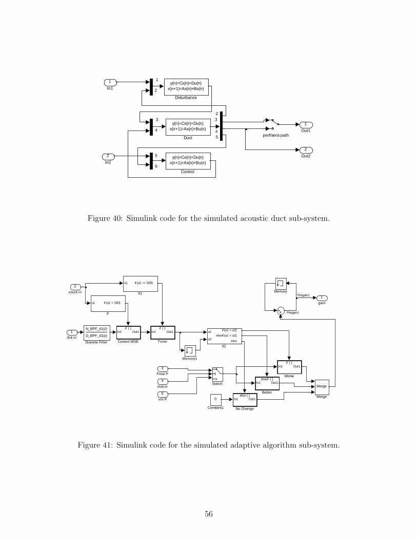
2

1

3

2

1

3

45

4

5

6

62

Out2

1Out1

perf/sens path

y(n)=Cx(n)+Du(n)x(n+1)=Ax(n)+Bu(n)

Duct

y(n)=Cx(n)+Du(n)x(n+1)=Ax(n)+Bu(n)

Disturbance

y(n)=Cx(n)+Du(n)x(n+1)=Ax(n)+Bu(n)

Control

2In2

1In1

Figure 40: Simulink code for the simulated acoustic duct sub-system.

1gain

if In1 Out1

Worse

if In1 Out1

Timer

Switch

else In1 Out1

No Change

Merge

Merge

Memory1

Memory

u1

u2

if (u1 > u2)elseif (u1 < u2)

elseIf2

u1 if (u1 == 500)

If1

u1 if (u1 > 100)

If

N_BPF_d1(z)

D_BPF_d1(z)

Discrete Filter

if In1 Out1

Current MSE

0

Constant1

elseif In1 Out1

Better5init P

4clok in

3Final P

2count in

1dist in

Pregain1

Pregain1

Figure 41: Simulink code for the simulated adaptive algorithm sub-system.

56

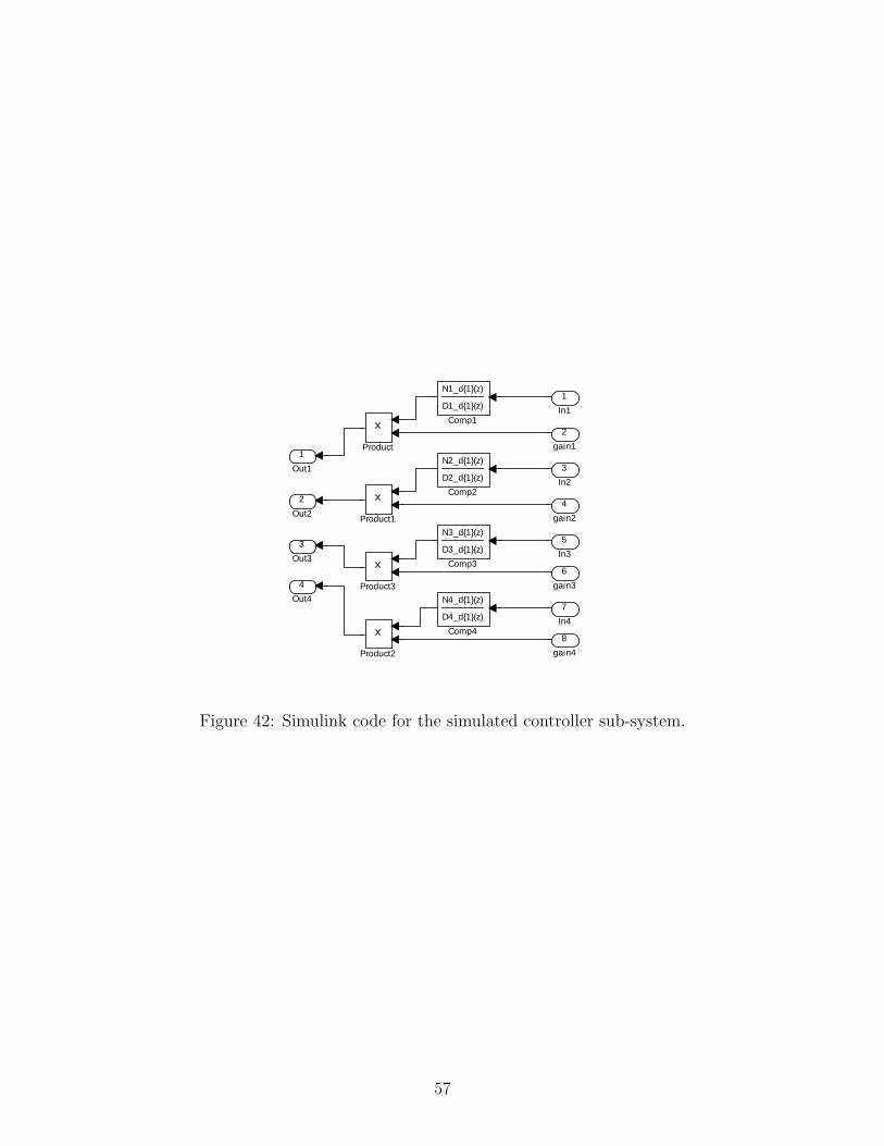
4Out4

3Out3

2Out2

1Out1

Product3

Product2

Product1

Product

N4_d1(z)

D4_d1(z)Comp4

N3_d1(z)

D3_d1(z)Comp3

N2_d1(z)

D2_d1(z)Comp2

N1_d1(z)

D1_d1(z)Comp1

8gain4

7In4

6gain3

5In3

4gain2

3In2

2gain1

1In1

Figure 42: Simulink code for the simulated controller sub-system.

57

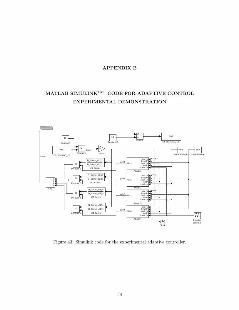
APPENDIX B

MATLAB SIMULINKTM CODE FOR ADAPTIVE CONTROL

EXPERIMENTAL DEMONSTRATION

RTI Data

Product1

Product 4

Product 3

Product 2

Product 1

N_Comp_d4(z)

D_Comp_d4(z)

M4 Comp

N_Comp_d3(z)

D_Comp_d3(z)

M3 Comp

N_Comp_d2(z)

D_Comp_d2(z)

M2 Comp

N_Comp_d1(z)

D_Comp_d1(z)

M1 Comp

5e-3

Initial Pertrub

-1

Gain

1e-4

Final Perturb

Divide

DAC

DS1104DAC_C1

ADC

DS1104ADC_C5

lim

CounterLimited

10

Constant2

10

Constant

Clock

Add

dist inFinal P

clock ininit P

count in

Out1

Adapt 4

dist inFinal P

clock ininit P

count in

Out1

Adapt 3

dist inFinal P

clock ininit P

count in

Out1

Adapt 2

dist inFinal P

clock ininit P

count in

Out1

Adapt 1

output

input

gain1

gain2

gain3

gain4

Figure 43: Simulink code for the experimental adaptive controller.

58

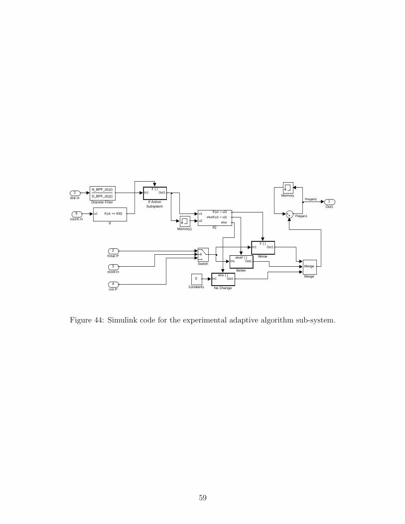
1Out1

if In1 Out1

Worse

Switch

else In1 Out1

No Change

Merge

Merge

Memory1

Memory

u1

u2

if (u1 > u2)elseif (u1 < u2)

elseIf2

if In1 Out1

If ActionSubsystem

u1 if (u1 == 500)

If

N_BPF_d1(z)

D_BPF_d1(z)

Discrete Filter

0

Constant1

elseif In1 Out1

Better

5count in

4init P

3clock in

2Final P

1dist in Pregain1

Pregain1

Figure 44: Simulink code for the experimental adaptive algorithm sub-system.

59

BIBLIOGRAPHY

[1] David A. Bies and Colin Hansen. Engineering Noise Control: Theory and Practice.Taylor and Francis Group, New York, 2003.

[2] C. B. Birdsong and C. J. Radcliffe. A compensated acoustic actuator for system withstrong dynamic pressure coupling. JVA, 121:89–94, January 1999.

[3] J. B. Bisnette, J. S. Vipperman, and D. D. Budney. Active noise control using phase-compensated, damped resonant filters. ASME IMECE, (2003-41831), November 15-212003. Washington, D.C.

[4] Jesse B. Bisnette. Active noise control using modally tuned phase-compensated filters.Master’s thesis, University of Pittsburgh, 2003.

[5] J. P. den Hartdog. Mechanical Vibrations. McGraw-Hill Book Company, New York, 4thedition, 1956.

[6] S. J. Elliot. Signal Processing for Active Control. Academic Press, New York, 2001.

[7] S. J. Estve and M. E. Johnson. Reduction of sound transmitted into a compositecylinder using distributed vibration absorbers and helmholtz resonators. Journal of theAcoustical Society of America, 112(6):2040–2048, 2002.

[8] F. J. Fahy and C. Schofield. A note on the interaction between a helmoltz resonatorand an acoustic mode of an enclosure. JVA, 72(3):365–378, April 1980.

[9] J. L. Fanson and T. K. Caughey. Positive position feedback control for large spacestructures. AIAA Journal, 28(4):717–724, April 1990.

[10] K. M. Farinholt and D. J. Leo. Acoustic modeling and control of conical enclosures.JVA, 125(1):2–11, 2003.

[11] Woon S. Gan and Sen M. Kuo. An integrated audio and active noise control headsets.IEEE, 48(2):242–247, May 2002.

[12] C. J. Goh and T. K. Caughey. On the stability problem caused by finite actuatordynamics in the collocated control of large space structures. Int. J. Control, 41(3):787–802, 1985.

60

[13] Edison J. Hahn and T. F. Edgar. A note on stability analysis using bode plots. ChemicalEngineering Education, 35(3):208–11, Summer 2001.

[14] Colin H. Hansen. Understanding Active Noise Cancellation. Spon Press, New York,2001.

[15] R. J. Bernhard J. M. De Bedout, M. A. Franchek and L. Mongeau. Adaptive-passivenoise control with self-tuning helmholtz resonators. JSV, 202(1):109–123, October 1997.

[16] A. G. Kelkar and H. R. Pota. Robust broadband control of acoustic duct. IEEE,1:273–278, September 2000.

[17] Lawrence E. Kinsler. Fundamental of acoustics. Wiley, New York, 1982.

[18] Theodore M. Kostek. Combining adaptive-pasive and fully active noise control in ducts.ASME Noise Control and Acoustics Division, 24:293–298, November 1997.

[19] Sen M. Kuo and Dennis R. Morgan. Active Noise Control Systems. John Wiley andSons, New York, 1996.

[20] Sen M. Kuo and Dennis R. Morgan. Review of DSP algorithms for active noise control.IEEE ICCA, (0-70803-6562-3/00), September 25-27 2000. Anchorage, Alaska.

[21] Steven A. Lane and Robert L. Clark. Dissipative feedback control of a reverberantenclosure using a constant volume velocity source. JVA, 120(3):987–993, 1998.

[22] M. D. Lutovac, D. J. Tosic, and B. L. Evans. Filter Design for Signal Processing.Prentice Hall, New Jersey, 2001.

[23] M. McEver and D. J. Leo. Autonomous vibration suppression using on-line pole-zeroidentification. JVA, 123:487–495, October 2001.

[24] Jerzy Moascianski and Zbigniew Ogonowski. Advanced control with Matlab andSimulink. Prentice Hall, Ellis Horwood, London, 1995.

[25] W. Neise and G.H. Koopmann. Reduction of centerifugal fan noise by use of resonators.Journal of Sound and Vibration, 73(2):297–308, November 1980.

[26] Young C. Park and Scott D. Sommerfeldt. Global attenuation of broadband noise fieldsusing energy density control. Journal of the Acoustic Society of America, 101:350–359,January 1997.

[27] H. R. Pota and A. G. Kelkar. Modeling and control of acoustic ducts. Transactions ofthe ASME, 213:2–10, January 2001.

[28] Singiresu S. Rao. Mechanical Vibrations. Prentice Hall, Upper Saddle River, New Jersey,4th edition, 2004.

61

[29] A. K. Smith, J. B. Bisnette, J. S. Vipperman, and D. D. Budny. Active noise controlusing phase-compensated, damped resonant filters. JVA, 2004. Accepted for publication.

[30] Adam K. Smith, Jeffrey S. Vipperman, and Daniel D. Budny. Adaptive resonant modeacoustic controller. IMECE, 2005. Accepted For Publication.

[31] M. E. Valkenburg. Analog Filter Design. Holt and Rinehart and Winston, Philadelphia,1982.

[32] Bernard Widrow and Samuel D. Stearns. Adaptive Signal Processing. Prentice Hall,Englewood Cliffs, New Jersy, 1985.

62