Adam Aurisano - Collider Detector at Fermilabaurisano/aurisano_cornell040312.pdf · 3 April 2012 Adam Aurisano, Texas A&M University 4 Supersymmetry Supersymmetry (SUSY) proposes

Search for New Physics in the Search for New Physics in the Exclusive Delayed Photon + MET Exclusive Delayed Photon + MET

Final StateFinal State

Adam AurisanoTexas A&M University

Cornell HEP Seminar3 April 2012

Adam Aurisano, Texas A&M University3 April 2012 2

OutlineOutline

Introduction Motivation Tools Overview of the Delayed Photon Analysis Backgrounds with Large Times and Cuts to

Get Rid of Them Background Estimation Results Conclusions


Standard ModelStandard Model

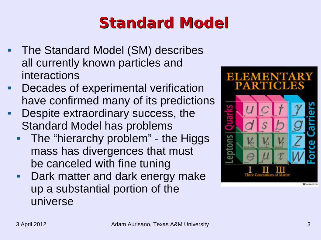
The Standard Model (SM) describes all currently known particles and interactions

Decades of experimental verification have confirmed many of its predictions

Despite extraordinary success, the Standard Model has problems

The “hierarchy problem” - the Higgs mass has divergences that must be canceled with fine tuning

Dark matter and dark energy make up a substantial portion of the universe


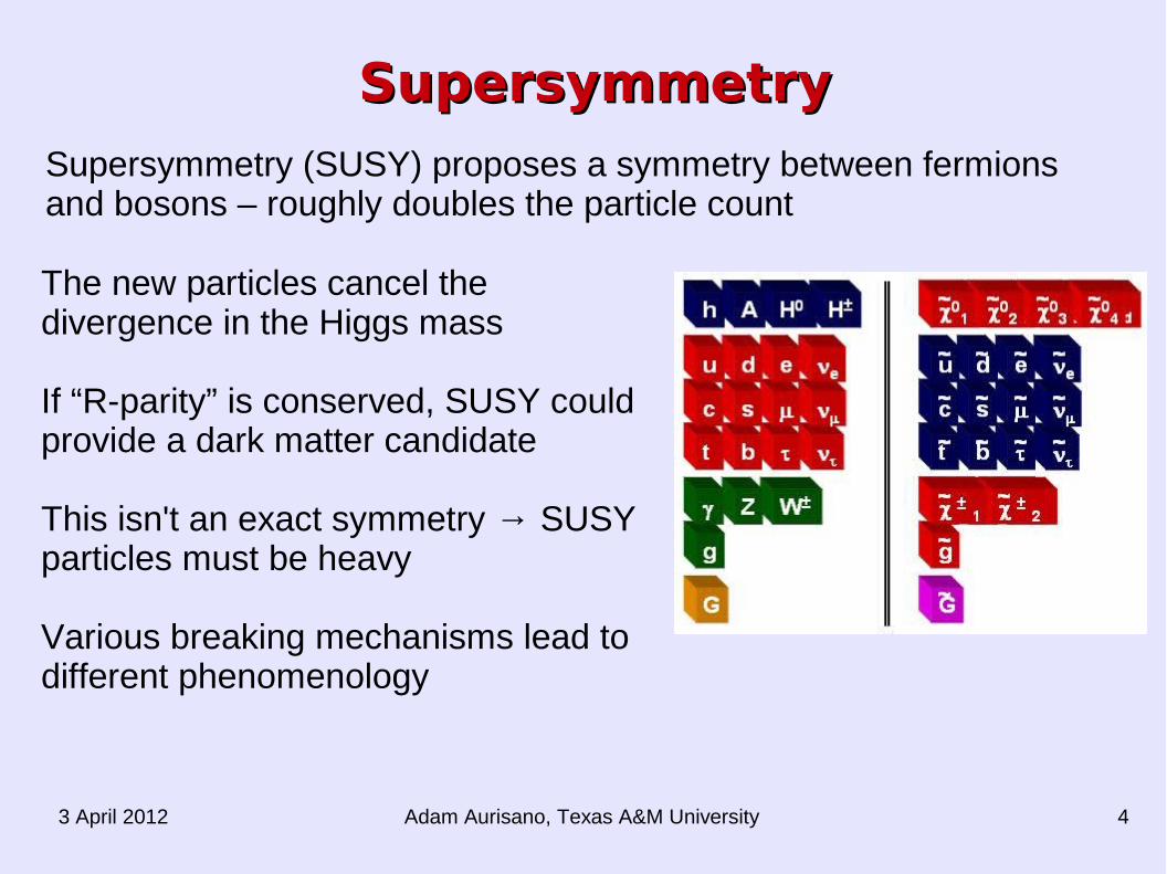
SupersymmetrySupersymmetrySupersymmetry (SUSY) proposes a symmetry between fermions and bosons – roughly doubles the particle count

The new particles cancel the divergence in the Higgs mass

If “R-parity” is conserved, SUSY could provide a dark matter candidate

This isn't an exact symmetry → SUSY particles must be heavy

Various breaking mechanisms lead to different phenomenology


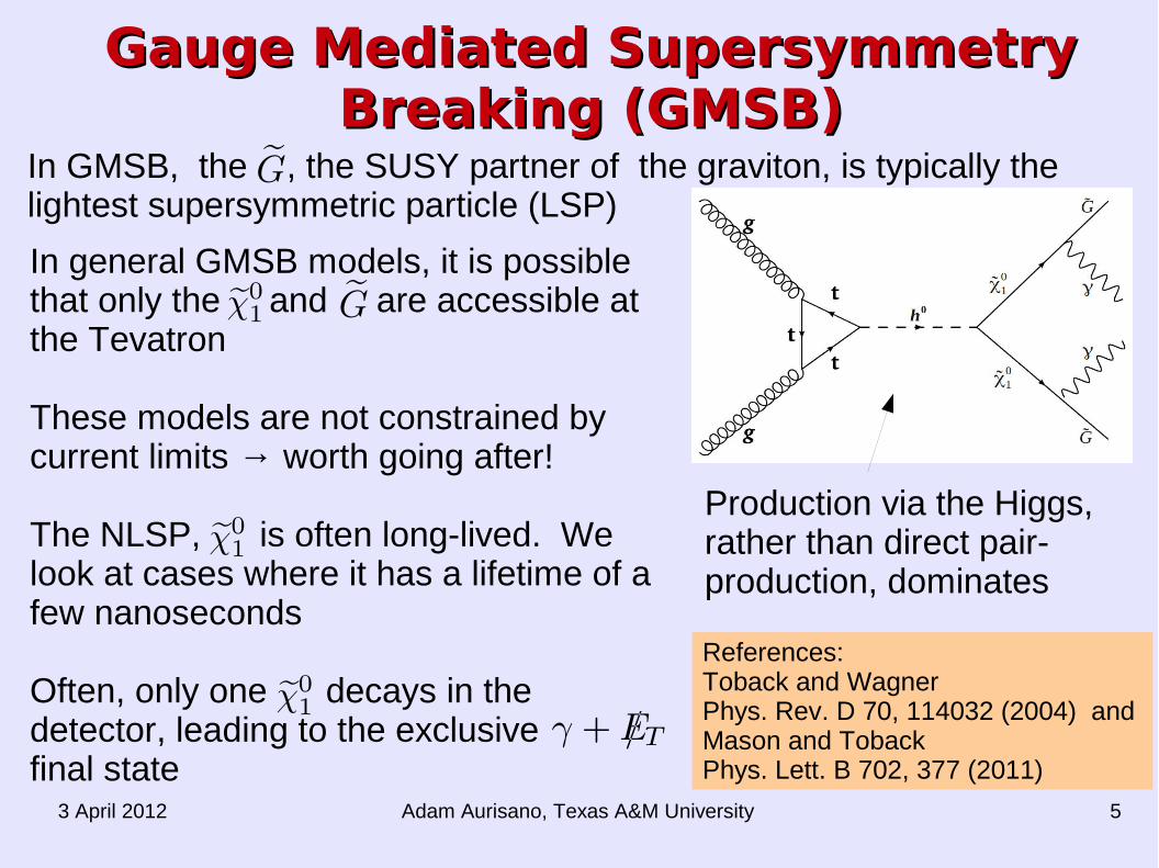
In general GMSB models, it is possible that only the and are accessible at the Tevatron

These models are not constrained by current limits → worth going after!

The NLSP, is often long-lived. We look at cases where it has a lifetime of a few nanoseconds

Often, only one decays in the detector, leading to the exclusive final state

In GMSB, the , the SUSY partner of the graviton, is typically the lightest supersymmetric particle (LSP)

Gauge Mediated Supersymmetry Gauge Mediated Supersymmetry Breaking (GMSB)Breaking (GMSB)

References:Toback and Wagner Phys. Rev. D 70, 114032 (2004) and Mason and TobackPhys. Lett. B 702, 377 (2011)

Production via the Higgs, rather than direct pair-production, dominates


TevatronTevatron

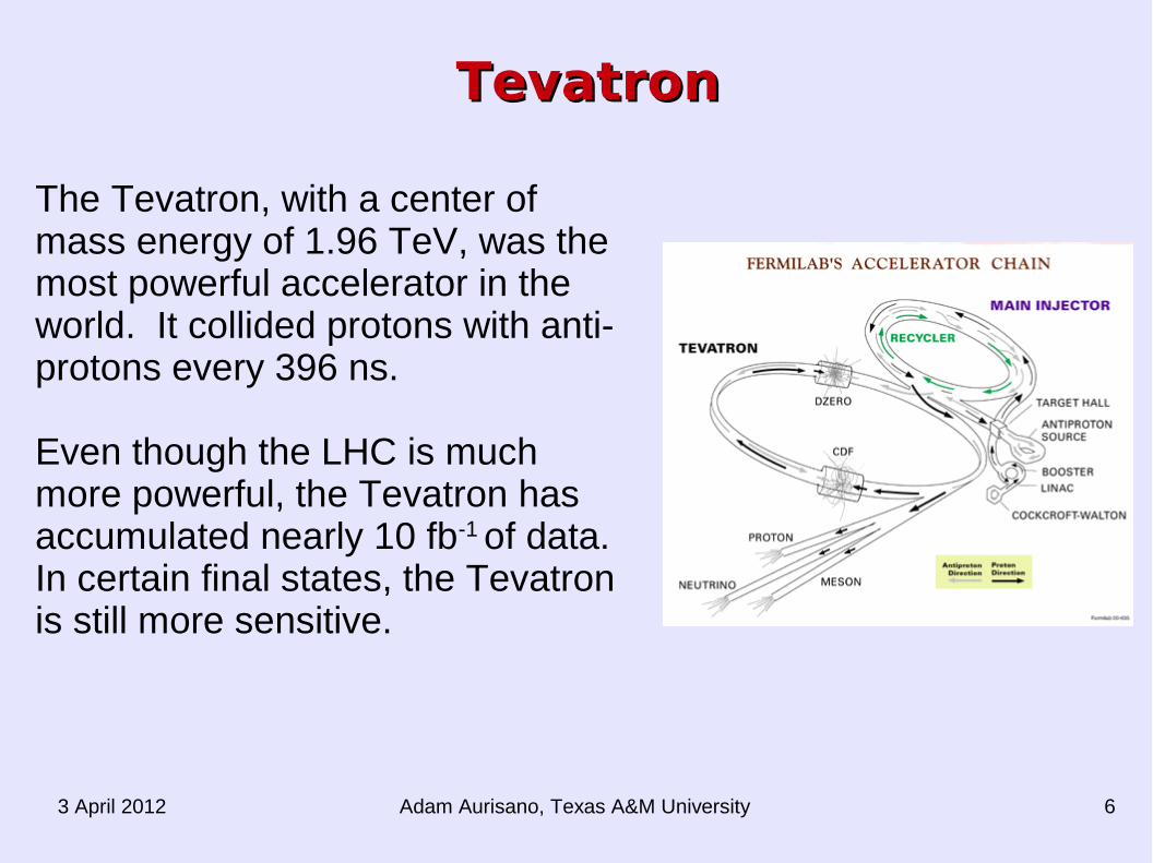
The Tevatron, with a center of mass energy of 1.96 TeV, was the most powerful accelerator in the world. It collided protons with anti-protons every 396 ns.

Even though the LHC is much more powerful, the Tevatron has accumulated nearly 10 fb-1 of data. In certain final states, the Tevatron is still more sensitive.


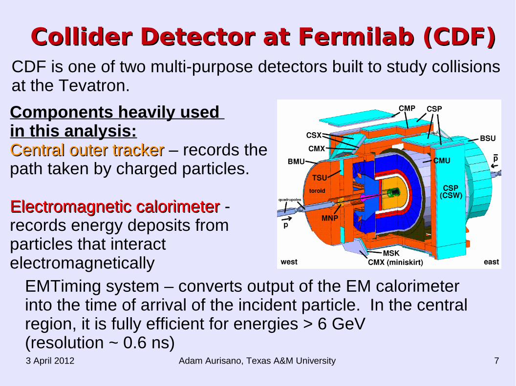
Collider Detector at Fermilab (CDF)Collider Detector at Fermilab (CDF)CDF is one of two multi-purpose detectors built to study collisions at the Tevatron.

Components heavily used in this analysis:Central outer trackerCentral outer tracker – records the path taken by charged particles.

Electromagnetic calorimeterElectromagnetic calorimeter -records energy deposits from particles that interactelectromagnetically

EMTiming system – converts output of the EM calorimeter into the time of arrival of the incident particle. In the central region, it is fully efficient for energies > 6 GeV (resolution ~ 0.6 ns)


Delayed PhotonsDelayed Photons

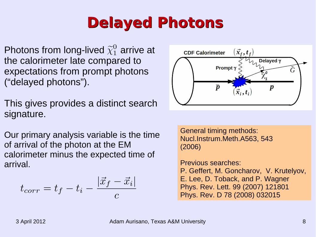
Photons from long-lived arrive at the calorimeter late compared to expectations from prompt photons (“delayed photons”).

This gives provides a distinct search signature.

Our primary analysis variable is the time of arrival of the photon at the EM calorimeter minus the expected time of arrival.

General timing methods:Nucl.Instrum.Meth.A563, 543(2006)

Previous searches:P. Geffert, M. Goncharov, V. Krutelyov, E. Lee, D. Toback, and P. WagnerPhys. Rev. Lett. 99 (2007) 121801Phys. Rev. D 78 (2008) 032015


Overview of the Delayed Photon Overview of the Delayed Photon Analysis: Final StateAnalysis: Final State

Exclusive delayed photon + MET final state:Require: (all E

T relative to Z = 0)

-Photon with ET > 45 GeV

-MET > 45 GeV-At least one space-time vertex with |Z| < 60 cm

Veto:-Extra calorimeter clusters with E

T > 15 GeV

-Tracks with PT > 10 GeV

-Tracks geometrically close to the photon-Standard Vertices with at least 3 tracks and |Z| > 60 cm-Additional cosmics and beam halo cuts


Overview of the Delayed Photon Overview of the Delayed Photon Analysis: BackgroundsAnalysis: Backgrounds

Standard Model Collision Sources

Non-Collision

•Cosmics •Beam Halo

As in published analyses, background estimation is data-driven.

Standard Model sources have different characteristics depending on whether we select a right or wrong vertex


Overview of the Delayed Photon Overview of the Delayed Photon Analysis: Analysis: Right Vertex DistributionRight Vertex Distribution

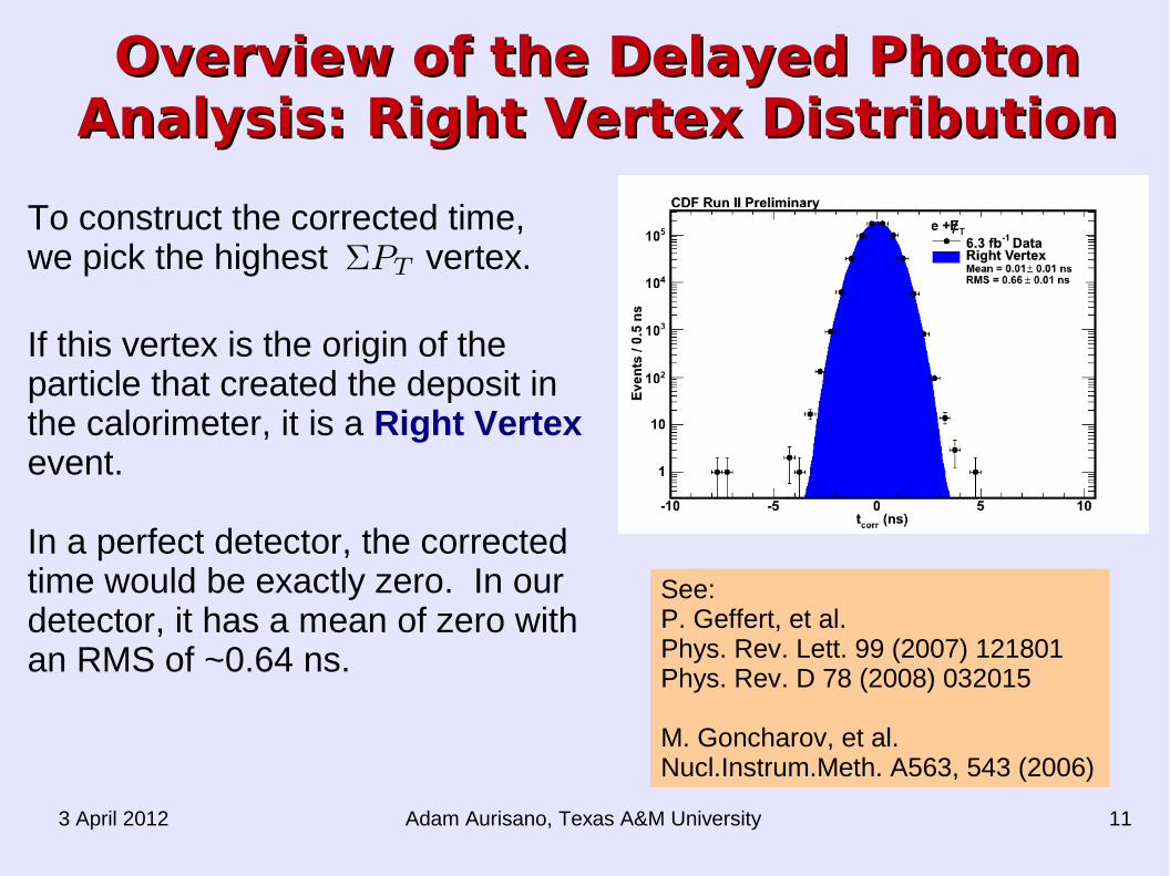
To construct the corrected time,we pick the highest

vertex.

If this vertex is the origin of the particle that created the deposit in the calorimeter, it is a Right Vertexevent.

In a perfect detector, the corrected time would be exactly zero. In our detector, it has a mean of zero with an RMS of ~0.64 ns.

See:P. Geffert, et al.Phys. Rev. Lett. 99 (2007) 121801Phys. Rev. D 78 (2008) 032015

M. Goncharov, et al.Nucl.Instrum.Meth. A563, 543 (2006)


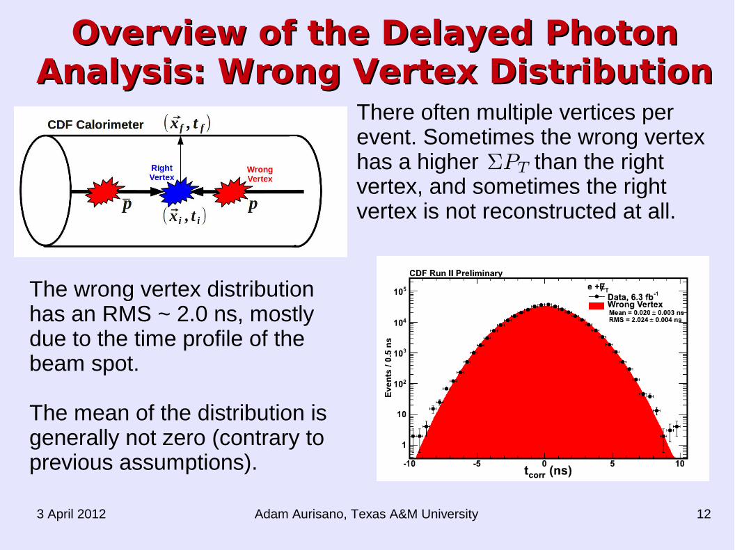
Overview of the Delayed Photon Overview of the Delayed Photon Analysis: Wrong Vertex DistributionAnalysis: Wrong Vertex Distribution

There often multiple vertices per event. Sometimes the wrong vertex has a higher than the right vertex, and sometimes the right vertex is not reconstructed at all.

The wrong vertex distribution has an RMS ~ 2.0 ns, mostly due to the time profile of the beam spot.

The mean of the distribution is generally not zero (contrary to previous assumptions).


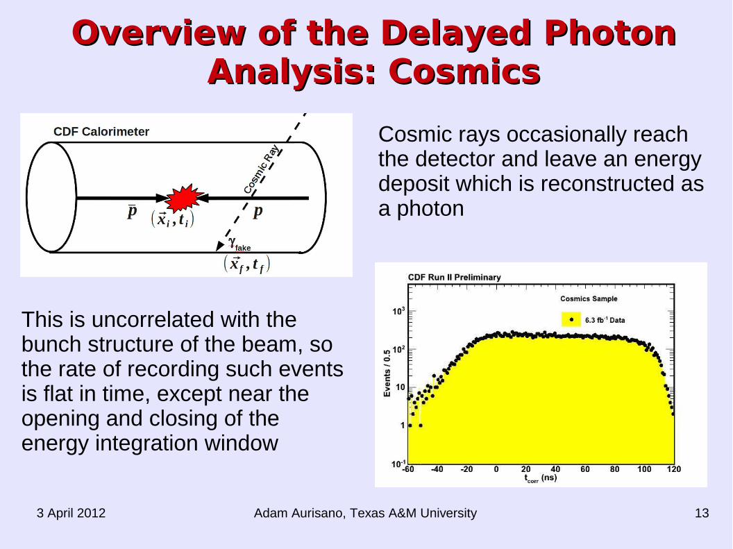
Overview of the Delayed Photon Overview of the Delayed Photon Analysis: CosmicsAnalysis: Cosmics

Cosmic rays occasionally reach the detector and leave an energy deposit which is reconstructed as a photon

This is uncorrelated with the bunch structure of the beam, so the rate of recording such events is flat in time, except near the opening and closing of the energy integration window


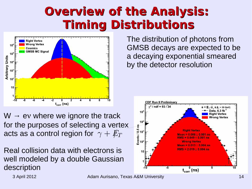
Overview of the Analysis: Overview of the Analysis: Timing DistributionsTiming Distributions

W → e where we ignore the track for the purposes of selecting a vertex acts as a control region for

Real collision data with electrons is well modeled by a double Gaussian description

The distribution of photons from GMSB decays are expected to be a decaying exponential smeared by the detector resolution


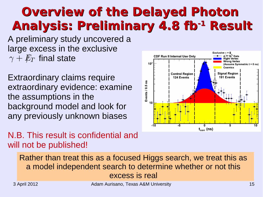
Overview of the Delayed Photon Overview of the Delayed Photon Analysis: Preliminary 4.8 fbAnalysis: Preliminary 4.8 fb-1-1 Result Result

A preliminary study uncovered a large excess in the exclusive final state

Extraordinary claims require extraordinary evidence: examine the assumptions in the background model and look for any previously unknown biases

N.B. This result is confidential and will not be published!

Rather than treat this as a focused Higgs search, we treat this as a model independent search to determine whether or not this

excess is real


Understanding the Preliminary Understanding the Preliminary ResultResult

We have found that initial assumption that the wrong-vertex mean = 0 is not correct

To develop a correct background estimate, we need to do three things

Identify effects which could lead to large times Develop new requirements which reduce any

biases Develop a method to measure any remaining

bias


Sources of Large Times from SM Sources of Large Times from SM BackgroundsBackgrounds

A number of effects can cause SM wrong vertex backgrounds to have large mean shifts.1) E

T Threshold Effect:

A distortion caused by events entering or leaving our sample due mis-measured E

T near the cut.

Topology Biases: 2) Fake photons: Fake photons tend to be biased to larger times due to being more likely at large path lengths.

3) Lost jets: Losing an object tends to happen at more extreme vertex Z positions (to allow the object to point out of the detector).

Next: examine these effect and show how to mitigate them


Sources of Large Time Events: Sources of Large Time Events: 1) E1) E

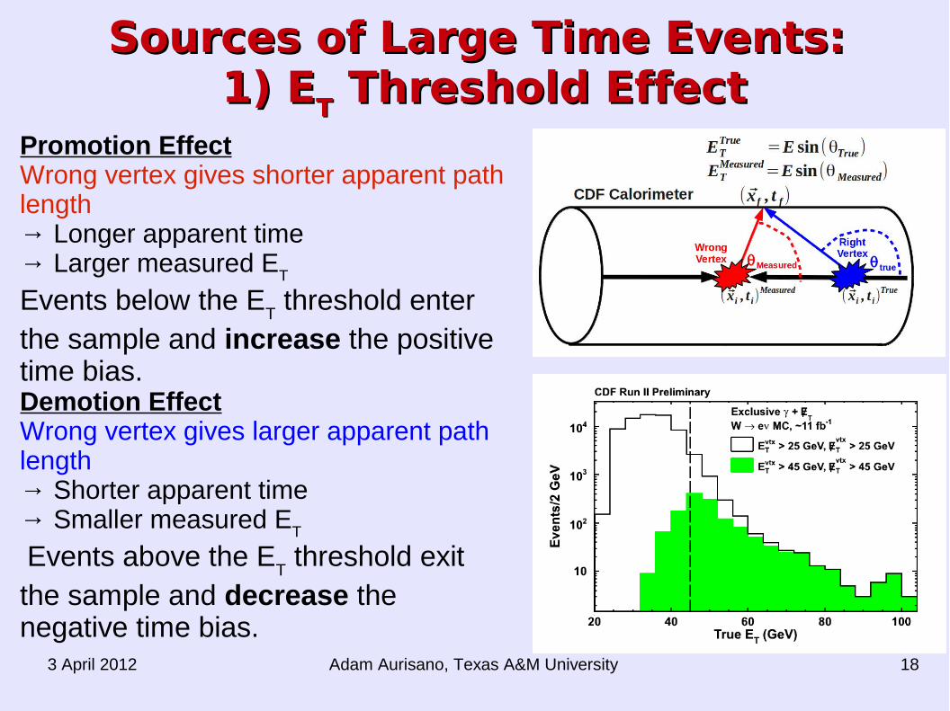
TT Threshold Effect Threshold EffectPromotion EffectWrong vertex gives shorter apparent path length→ Longer apparent time→ Larger measured E

T

Events below the ET threshold enter

the sample and increase the positive time bias.Demotion EffectWrong vertex gives larger apparent path length→ Shorter apparent time→ Smaller measured E

T

Events above the ET threshold exit

the sample and decrease the negative time bias.


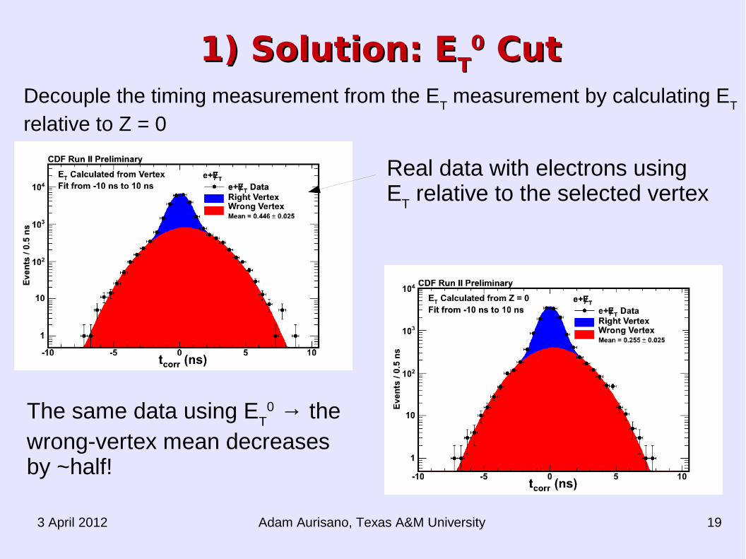
1) Solution: E1) Solution: ETT00 Cut Cut

Decouple the timing measurement from the ET measurement by calculating E

T

relative to Z = 0

Real data with electrons using E

T relative to the selected vertex

The same data using ET

0 → the wrong-vertex mean decreases by ~half!


Sources of Large Time Events: Sources of Large Time Events: 2) Fake Photons2) Fake Photons

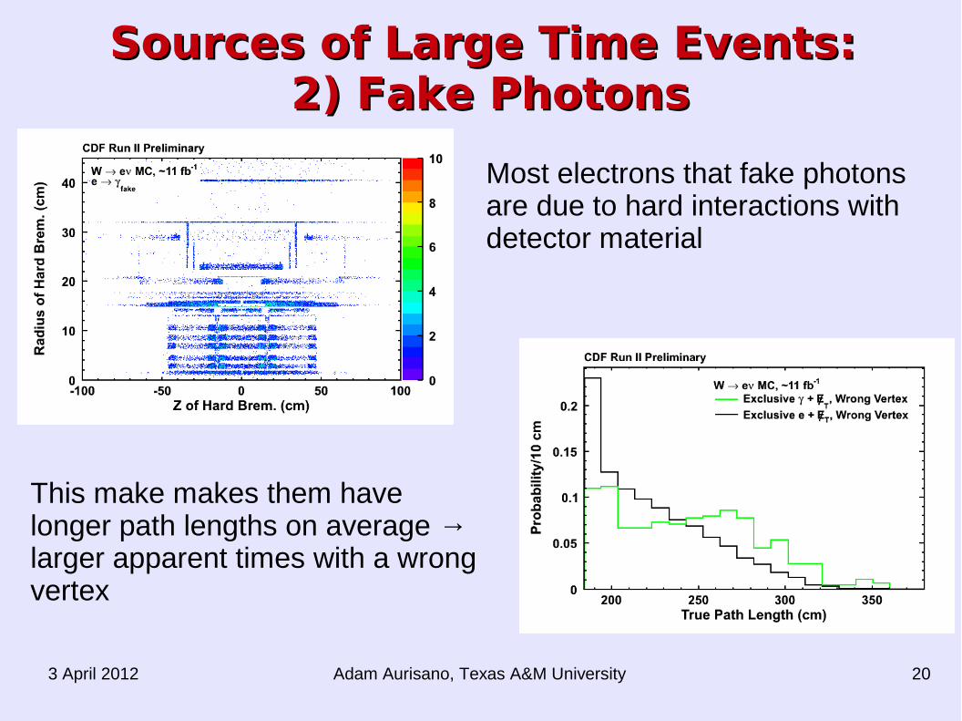
Most electrons that fake photons are due to hard interactions with detector material

This make makes them have longer path lengths on average → larger apparent times with a wrong vertex


2) Solution:2) Solution:RRpullpull Cut Cut

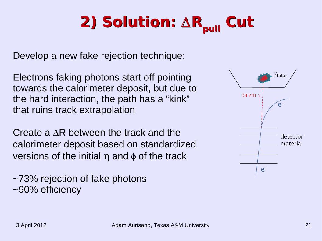
Develop a new fake rejection technique:

Electrons faking photons start off pointing towards the calorimeter deposit, but due to the hard interaction, the path has a “kink” that ruins track extrapolation

Create a R between the track and the calorimeter deposit based on standardized versions of the initial andof the track

~73% rejection of fake photons~90% efficiency


Sources of Large Time Events:Sources of Large Time Events:3) Large |Z| Production3) Large |Z| Production

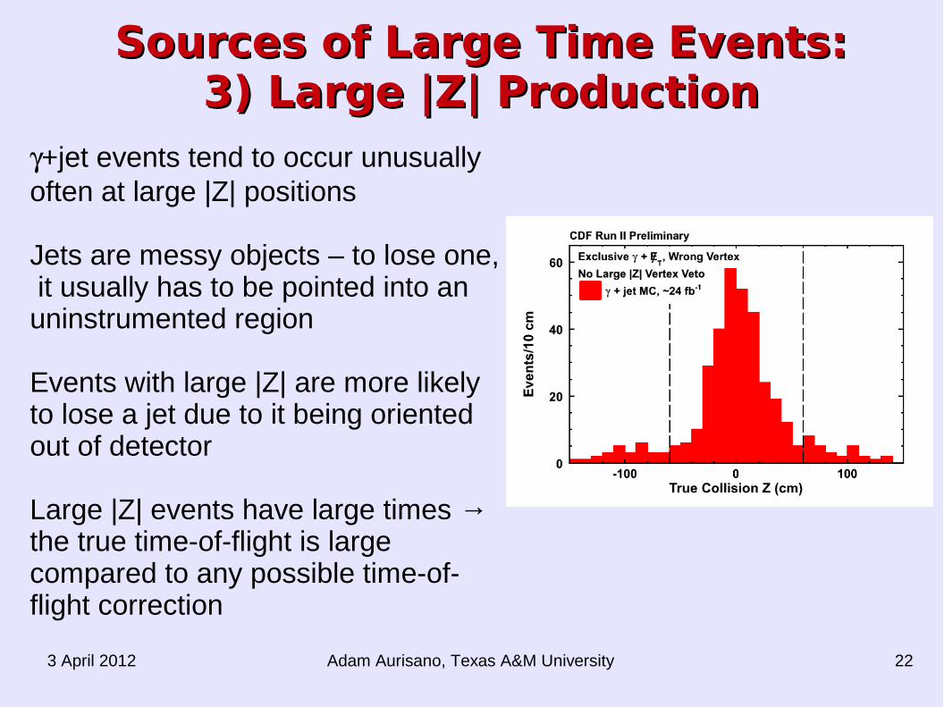
+jet events tend to occur unusually often at large |Z| positions

Jets are messy objects – to lose one, it usually has to be pointed into an uninstrumented region

Events with large |Z| are more likely to lose a jet due to it being oriented out of detector

Large |Z| events have large times → the true time-of-flight is large compared to any possible time-of-flight correction


3) Solution: Large |Z| Veto3) Solution: Large |Z| Veto

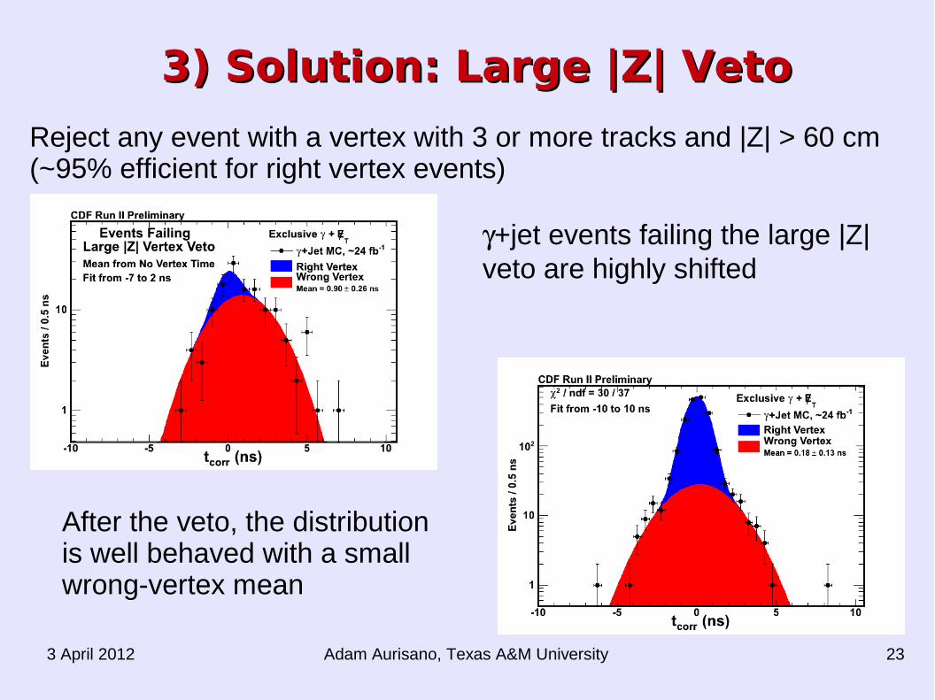
Reject any event with a vertex with 3 or more tracks and |Z| > 60 cm (~95% efficient for right vertex events)

+jet events failing the large |Z| veto are highly shifted

After the veto, the distribution is well behaved with a small wrong-vertex mean


Predicting Background Events in the SigPredicting Background Events in the Sig--nal Region From the Wrong-Vertex Mean nal Region From the Wrong-Vertex Mean

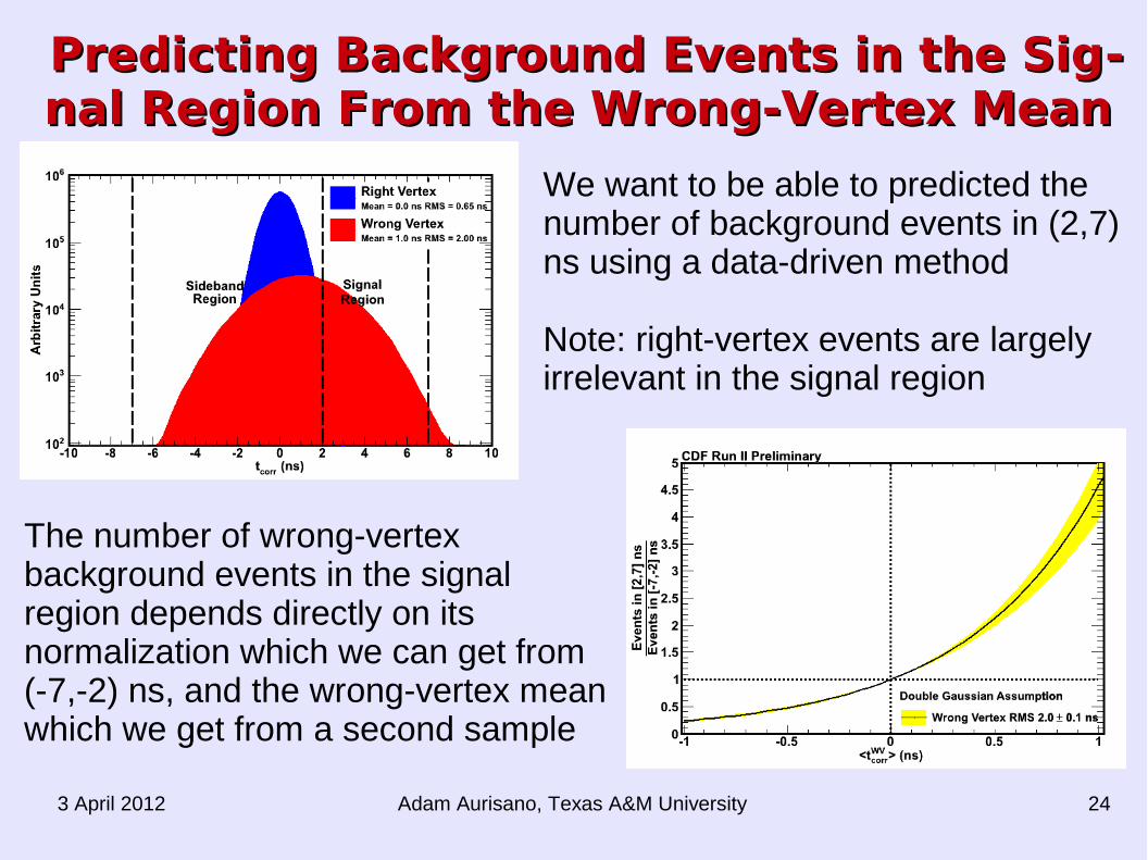
We want to be able to predicted the number of background events in (2,7) ns using a data-driven method

Note: right-vertex events are largely irrelevant in the signal region

The number of wrong-vertex background events in the signal region depends directly on its normalization which we can get from (-7,-2) ns, and the wrong-vertex mean which we get from a second sample


Checking the Double Gaussian Checking the Double Gaussian Approximation with Lots of DatasetsApproximation with Lots of Datasets

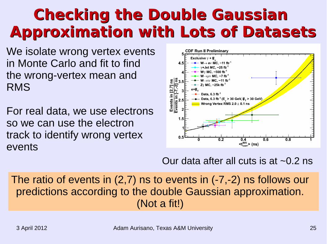
We isolate wrong vertex events in Monte Carlo and fit to find the wrong-vertex mean and RMS

For real data, we use electrons so we can use the electron track to identify wrong vertex events

The ratio of events in (2,7) ns to events in (-7,-2) ns follows our predictions according to the double Gaussian approximation.

(Not a fit!)

Our data after all cuts is at ~0.2 ns


Estimating the Wrong Vertex MeanEstimating the Wrong Vertex Mean

We want to be able to predict the number of events in the signal region only using various sideband region

If we know the wrong-vertex mean, we have enough information in (-7, -2) ns to make the estimation

How can we find the wrong-vertex mean? Fitting in (-7, 2) ns does not have enough in-

formation → we need an additional handle We find an addition handle in the no vertex

timing distribution.


Estimating the Wrong-Vertex Mean Estimating the Wrong-Vertex Mean From the No-Vertex Sample From the No-Vertex Sample

Create an orthogonal sample consisting of events passing all cuts except the good vertex requirement, and construct the corrected time around the center of the vertex distribution, Z = 0 and T = 0, to minimize the overall wrongness.

Because RMS ZWV ~ 28 cm, most |ZWV| are small compared to RCES → the time-of-flight from a wrong vertex is almost the same as the time-of-flight from Z = 0.

As long as the physics dependent quantities (ZRV and ZCES) are similar in the wrong and no-vertex samples, their means should be very close.


Does This Assumption Work?Does This Assumption Work?

The no-vertex mean well predicts the number of events in the signal region for all control samples

Check with both Monte Carlo and electrons in real data.

All samples show good agreement between the fitted no-vertex and wrong-vertex means


Effect of Combining Collision Effect of Combining Collision Background SourcesBackground Sources

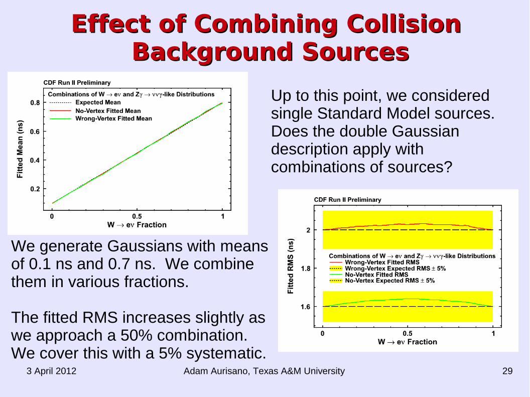
Up to this point, we considered single Standard Model sources. Does the double Gaussian description apply with combinations of sources?

We generate Gaussians with means of 0.1 ns and 0.7 ns. We combine them in various fractions.

The fitted RMS increases slightly as we approach a 50% combination. We cover this with a 5% systematic.


Putting It All Together: Putting It All Together: Likelihood FitLikelihood Fit

Estimate the number of background events in the signal region using a combined likelihood fit to the sideband regions extrapolated to the signal region

Good vertex: (-7,2) ns and (20,80) ns No vertex: (-3.5, 3.5) ns and (20,80) ns

Include systematic uncertainties as constraint terms:

Right-vertex mean = 0.0 0.05 ns Right-vertex RMS = 0.64 0.05 ns Wrong-vertex mean = No-vertex mean 0.08 ns Wrong-vertex RMS = 2.0 0.1 ns


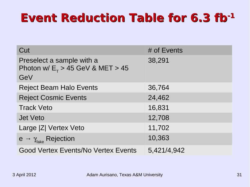
Cut # of Events

Preselect a sample with a Photon w/ E

T > 45 GeV & MET > 45

GeV

38,291

Reject Beam Halo Events 36,764

Reject Cosmic Events 24,462

Track Veto 16,831

Jet Veto 12,708

Large |Z| Vertex Veto 11,702

e → fake

Rejection 10,363

Good Vertex Events/No Vertex Events 5,421/4,942

Event Reduction Table for 6.3 fbEvent Reduction Table for 6.3 fb-1-1


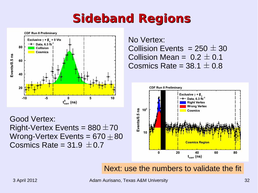
Sideband RegionsSideband Regions

No Vertex:Collision Events = 250 30Collision Mean = 0.2 0.1Cosmics Rate = 38.1 0.8

Good Vertex:Right-Vertex Events = 880 70Wrong-Vertex Events = 670 80Cosmics Rate = 31.9 0.7

Next: use the numbers to validate the fit


Validating the Likelihood FitValidating the Likelihood Fit

Generate ideal pseudo-experiments varying parameters within their systematic uncertainties

Generate more realistic pseudo-experiments from full MC of the three largest SM backgrounds

Sample at the statistics level seen in data Add the expected level of cosmics to the good and no

vertex distributions


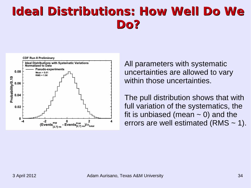
Ideal Distributions: How Well Do We Ideal Distributions: How Well Do We Do?Do?

All parameters with systematic uncertainties are allowed to vary within those uncertainties.

The pull distribution shows that with full variation of the systematics, the fit is unbiased (mean ~ 0) and the errors are well estimated (RMS ~ 1).


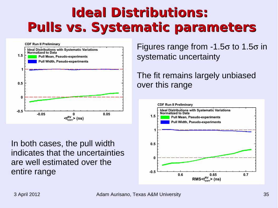
Ideal Distributions: Ideal Distributions: Pulls vs. Systematic parametersPulls vs. Systematic parameters

Figures range from -1.5 to 1.5 in systematic uncertainty

The fit remains largely unbiased over this range

In both cases, the pull width indicates that the uncertainties are well estimated over the entire range


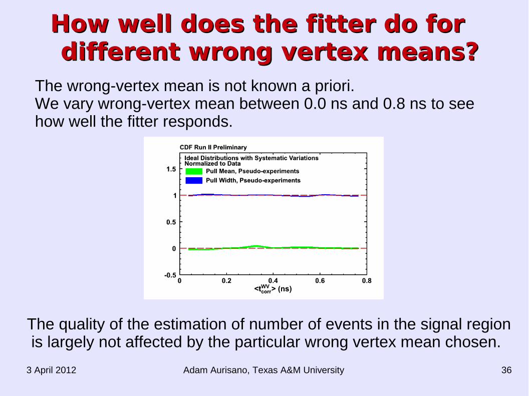
How well does the fitter do for How well does the fitter do for different wrong vertex means?different wrong vertex means?

The wrong-vertex mean is not known a priori. We vary wrong-vertex mean between 0.0 ns and 0.8 ns to see how well the fitter responds.

The quality of the estimation of number of events in the signal region is largely not affected by the particular wrong vertex mean chosen.


How well do we do when How well do we do when we combine fully we combine fully

simulated MC samples?simulated MC samples?We take Z, W → e, and +jet MC in random fractions.

Pull distribution: largely unbiased and the errors well estimated.

Double Gaussian approximation is very successful, even under worse case combinations.

Fit uncertainty ~23 counts.


ResultsResults

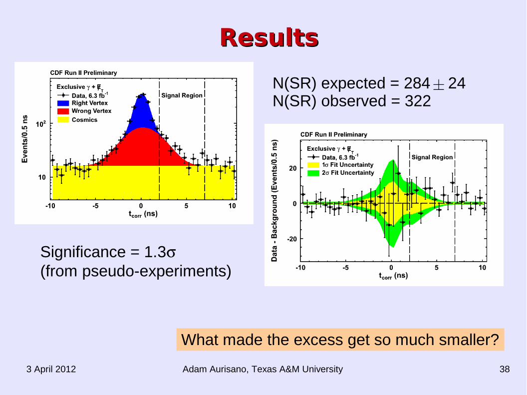
N(SR) expected = 284 24N(SR) observed = 322

Significance = 1.3 (from pseudo-experiments)

What made the excess get so much smaller?


Our new requirements decreased the worst bi-ases

W → e MC had the worst wrong-vertex mean (~0.8 ns), and it was originally the dominant background. After the R

pull cut, it is much less important

Our background estimation techniques are much better now

The wrong-vertex mean in the 4.8 fb-1 sample was very large and our previous method assumed it was zero

With our old cuts, this method would not have worked

What Happened to the Excess?What Happened to the Excess?


ConclusionsConclusions

Studied a previous excess in delayed photons and uncovered a number of previously un-known biases

Used new requirements to minimize those bi-ases in a way that is very efficient for any sig-nal

Developed a data driven method to estimate background contributions

A modest excess remains Now on to publication!


BackupsBackups


Overview of the Delayed Photon Overview of the Delayed Photon Analysis: Photon TimingAnalysis: Photon Timing

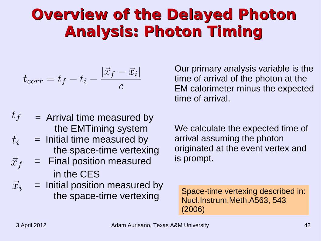
Our primary analysis variable is the time of arrival of the photon at the EM calorimeter minus the expected time of arrival.

We calculate the expected time of arrival assuming the photon originated at the event vertex and is prompt.

= Arrival time measured by the EMTiming system

= Initial time measured by the space-time vertexing

= Final position measured

in the CES = Initial position measured by the space-time vertexing Space-time vertexing described in:

Nucl.Instrum.Meth.A563, 543(2006)


Overview of the Delayed Photon Overview of the Delayed Photon Analysis: Satellite BunchesAnalysis: Satellite Bunches

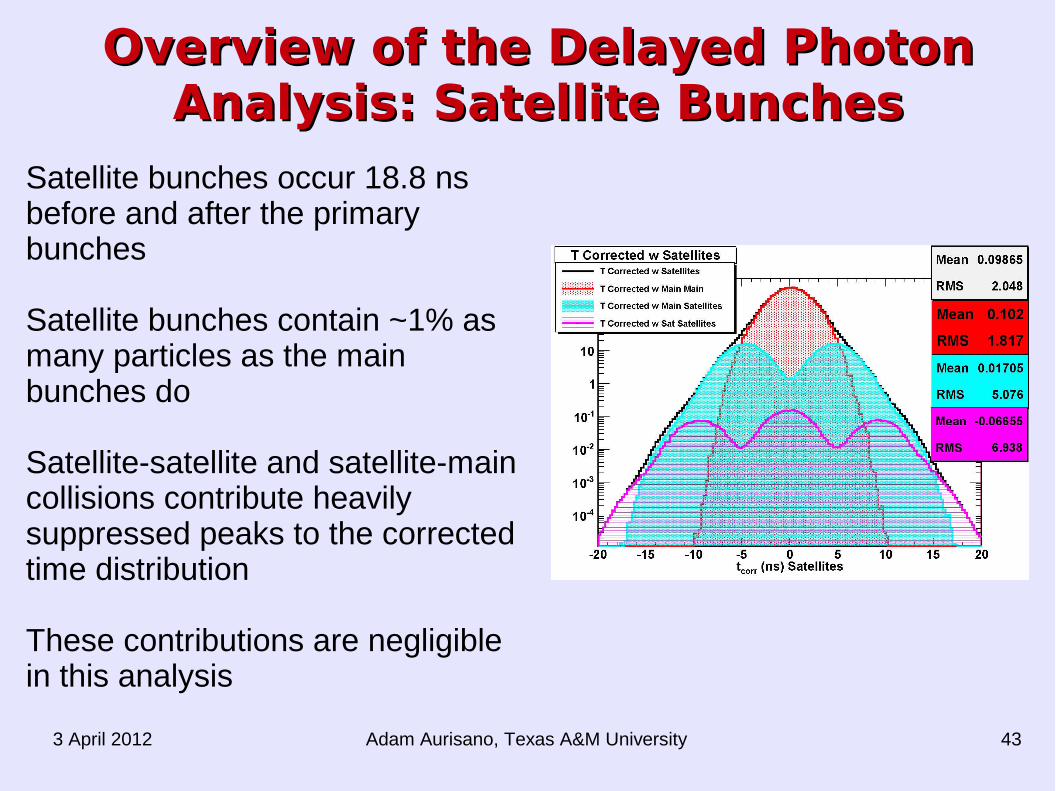
Satellite bunches occur 18.8 ns before and after the primary bunches

Satellite bunches contain ~1% as many particles as the main bunches do

Satellite-satellite and satellite-main collisions contribute heavily suppressed peaks to the corrected time distribution

These contributions are negligible in this analysis


Overview of the Delayed Photon Overview of the Delayed Photon Analysis: Beam HaloAnalysis: Beam Halo

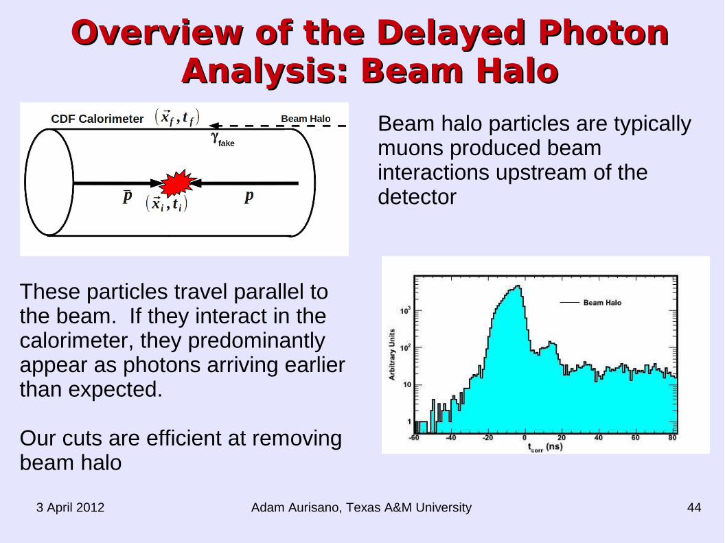
Beam halo particles are typically muons produced beam interactions upstream of the detector

These particles travel parallel to the beam. If they interact in the calorimeter, they predominantly appear as photons arriving earlier than expected.

Our cuts are efficient at removing beam halo


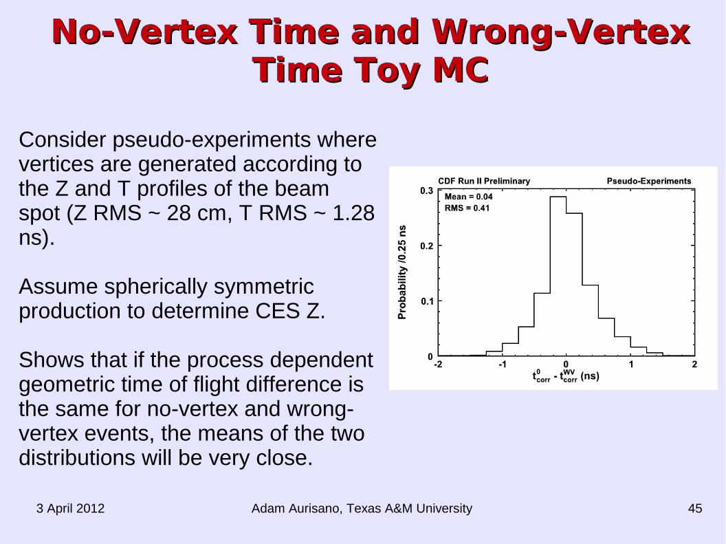
No-Vertex Time and Wrong-Vertex No-Vertex Time and Wrong-Vertex Time Toy MCTime Toy MC

Consider pseudo-experiments where vertices are generated according to the Z and T profiles of the beam spot (Z RMS ~ 28 cm, T RMS ~ 1.28 ns).

Assume spherically symmetric production to determine CES Z.

Shows that if the process dependent geometric time of flight difference is the same for no-vertex and wrong-vertex events, the means of the two distributions will be very close.


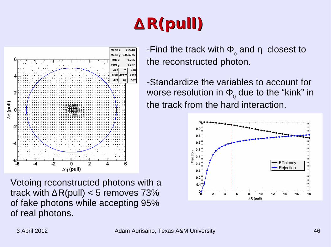
∆∆ R(pull)R(pull)

-Find the track with Φo and η closest to

the reconstructed photon.

-Standardize the variables to account for worse resolution in Φ

0 due to the “kink” in

the track from the hard interaction.

Vetoing reconstructed photons with a track with ∆R(pull) < 5 removes 73% of fake photons while accepting 95% of real photons.


Predicting N(SR)/N(CR) From No Predicting N(SR)/N(CR) From No Vertex MeanVertex Mean

N(SR)/N(CR) follows the prediction from the no-vertex mean as well as for the wrong-vertex mean → we can use the no-vertex mean as proxy for the wrong-vertex mean.

We isolate no vertex events in Monte Carlo and electron data and fit to find the no vertex mean.

The RMS of the no-vertex distribution does not depend on the mean of the distribution.


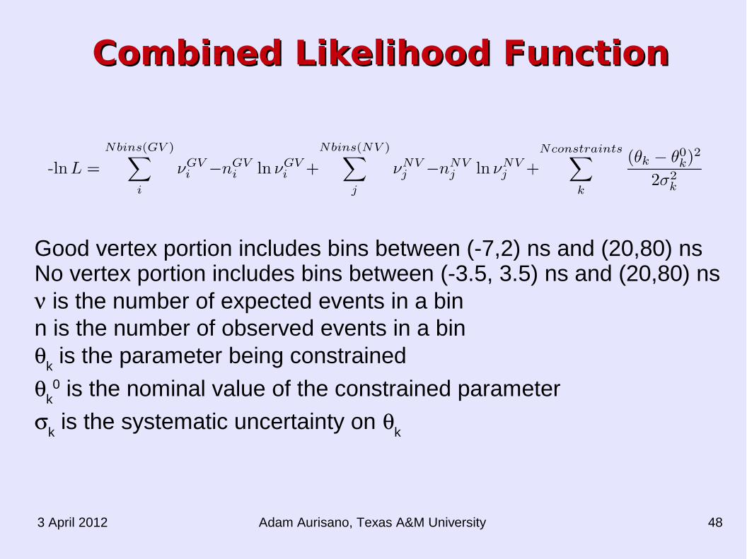
Combined Likelihood FunctionCombined Likelihood Function

Good vertex portion includes bins between (-7,2) ns and (20,80) nsNo vertex portion includes bins between (-3.5, 3.5) ns and (20,80) ns is the number of expected events in a binn is the number of observed events in a bin

k is the parameter being constrained

k0 is the nominal value of the constrained parameter

k is the systematic uncertainty on

k


COT Track tCOT Track t00 Corrections Corrections


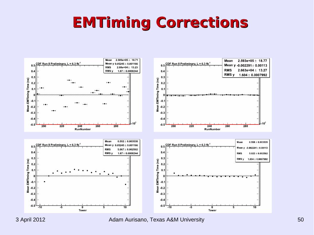
EMTiming CorrectionsEMTiming Corrections


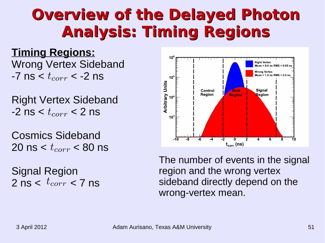
Overview of the Delayed Photon Overview of the Delayed Photon Analysis: Analysis: Timing RegionsTiming Regions

Timing Regions:Wrong Vertex Sideband-7 ns < < -2 ns

Right Vertex Sideband-2 ns < < 2 ns

Cosmics Sideband20 ns < < 80 ns

Signal Region2 ns < < 7 ns

The number of events in the signal region and the wrong vertex sideband directly depend on the wrong-vertex mean.


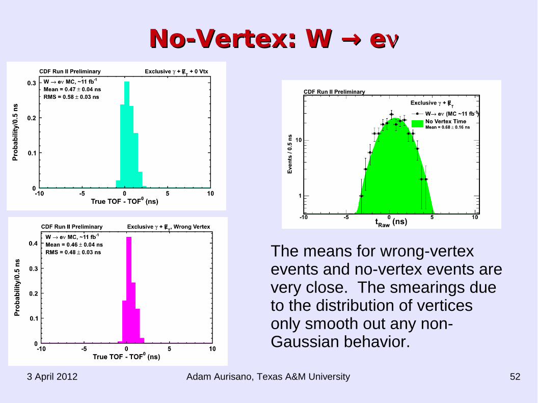
No-Vertex: W e→No-Vertex: W e→

The means for wrong-vertex events and no-vertex events are very close. The smearings due to the distribution of vertices only smooth out any non-Gaussian behavior.


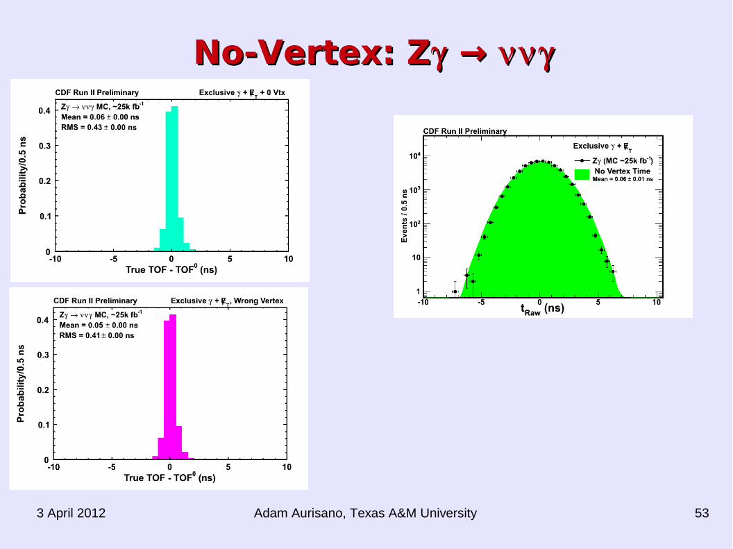
No-Vertex: ZNo-Vertex: Z → →


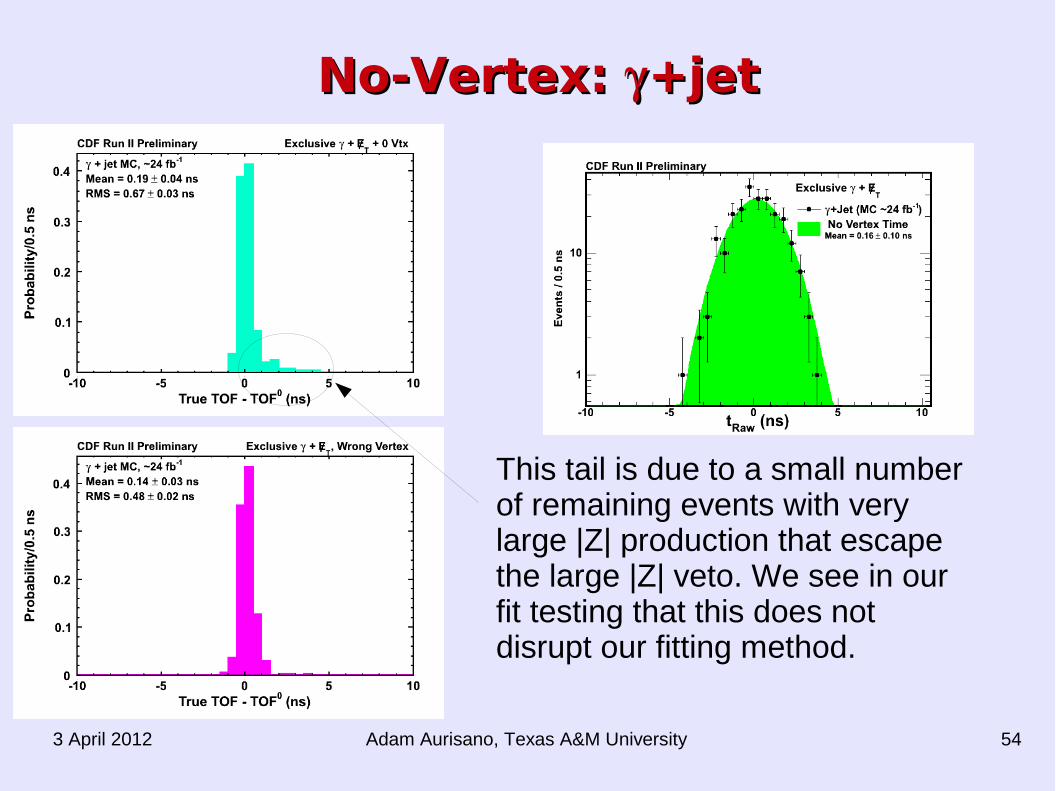
No-Vertex:No-Vertex:+jet+jet

This tail is due to a small number of remaining events with very large |Z| production that escape the large |Z| veto. We see in our fit testing that this does not disrupt our fitting method.


Overview of the Delayed Photon Overview of the Delayed Photon Analysis: Wrong Vertex MeanAnalysis: Wrong Vertex Mean

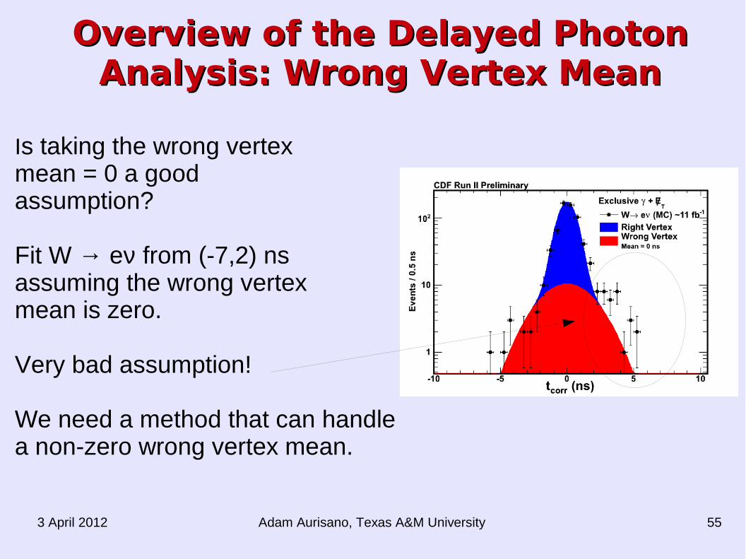
Is taking the wrong vertex mean = 0 a good assumption?

Fit W → eν from (-7,2) ns assuming the wrong vertex mean is zero.

Very bad assumption!

We need a method that can handlea non-zero wrong vertex mean.


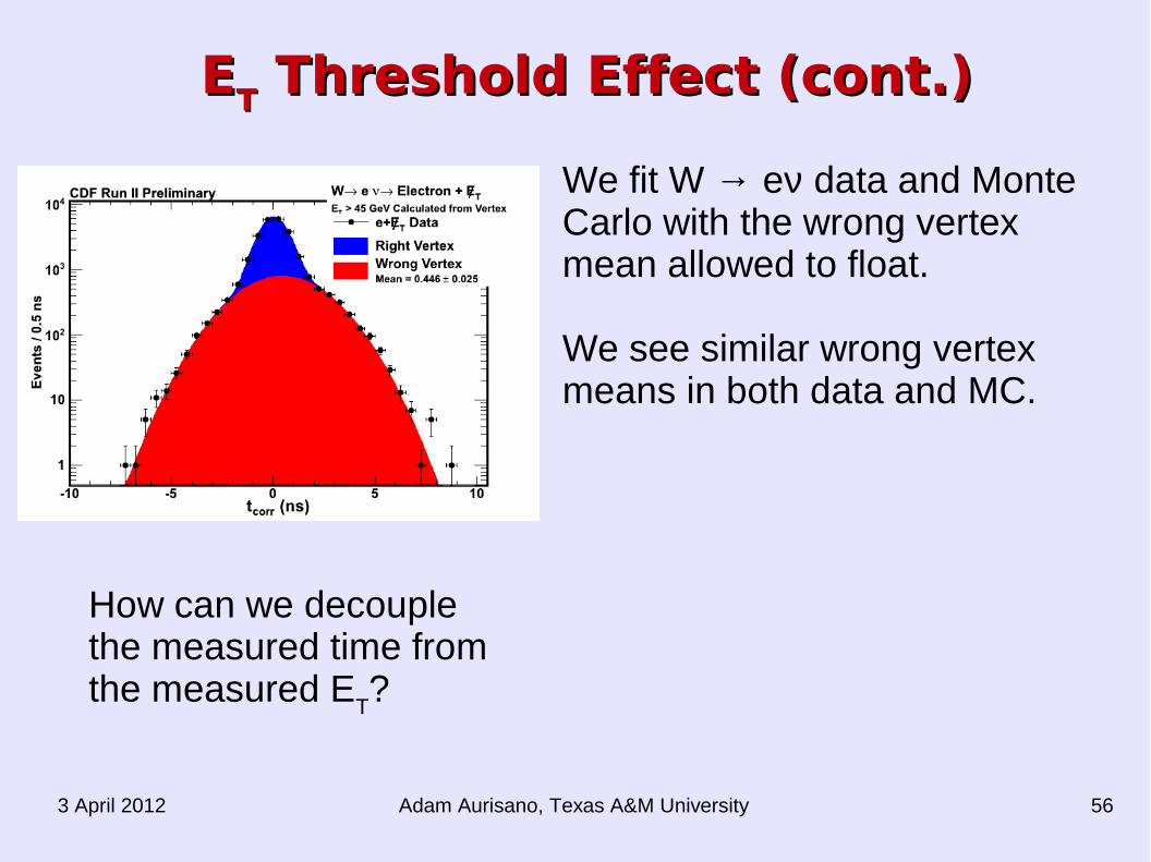
How can we decouplethe measured time from the measured E

T?

EETT Threshold Effect (cont.) Threshold Effect (cont.)

We fit W → eν data and Monte Carlo with the wrong vertex mean allowed to float.

We see similar wrong vertex means in both data and MC.


EETT00 Cut Cut

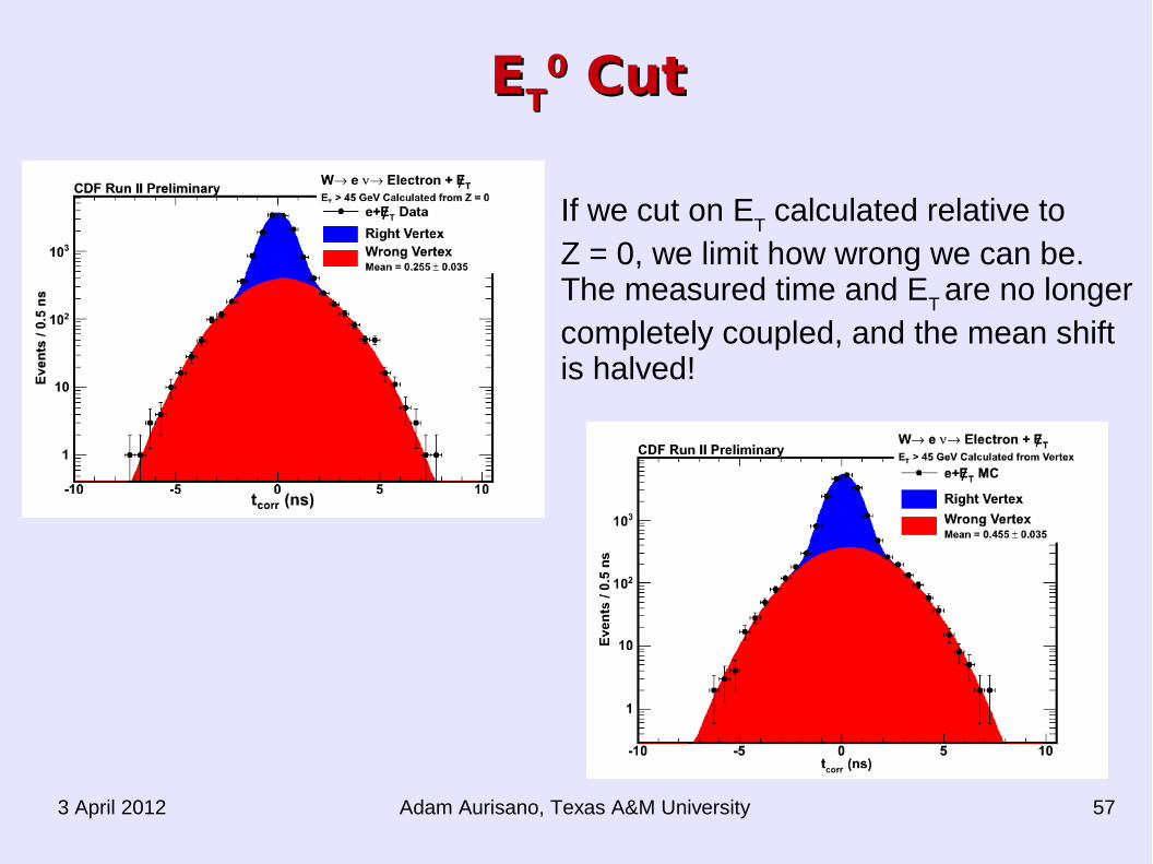
If we cut on ET calculated relative to

Z = 0, we limit how wrong we can be. The measured time and E

T are no longer

completely coupled, and the mean shift is halved!


Effect 2: Fake PhotonsEffect 2: Fake Photons

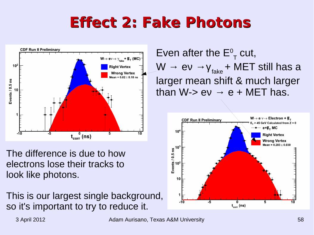
Even after the E0T cut,

W → eν →γfake

+ MET still has alarger mean shift & much larger than W-> eν → e + MET has.

The difference is due to how electrons lose their tracks to look like photons.

This is our largest single background,so it's important to try to reduce it.


Fake ReductionFake Reduction

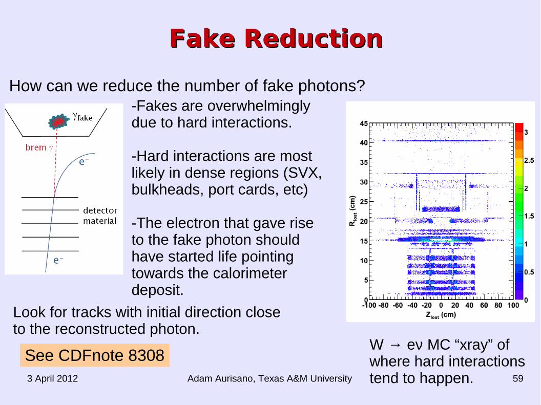
How can we reduce the number of fake photons?

W → eν MC “xray” of where hard interactions tend to happen.

-Fakes are overwhelminglydue to hard interactions.

-Hard interactions are mostlikely in dense regions (SVX, bulkheads, port cards, etc)

-The electron that gave riseto the fake photon should have started life pointing towards the calorimeter deposit.

Look for tracks with initial direction close to the reconstructed photon.

See CDFnote 8308


Effect 3: Lost ObjectsEffect 3: Lost Objects

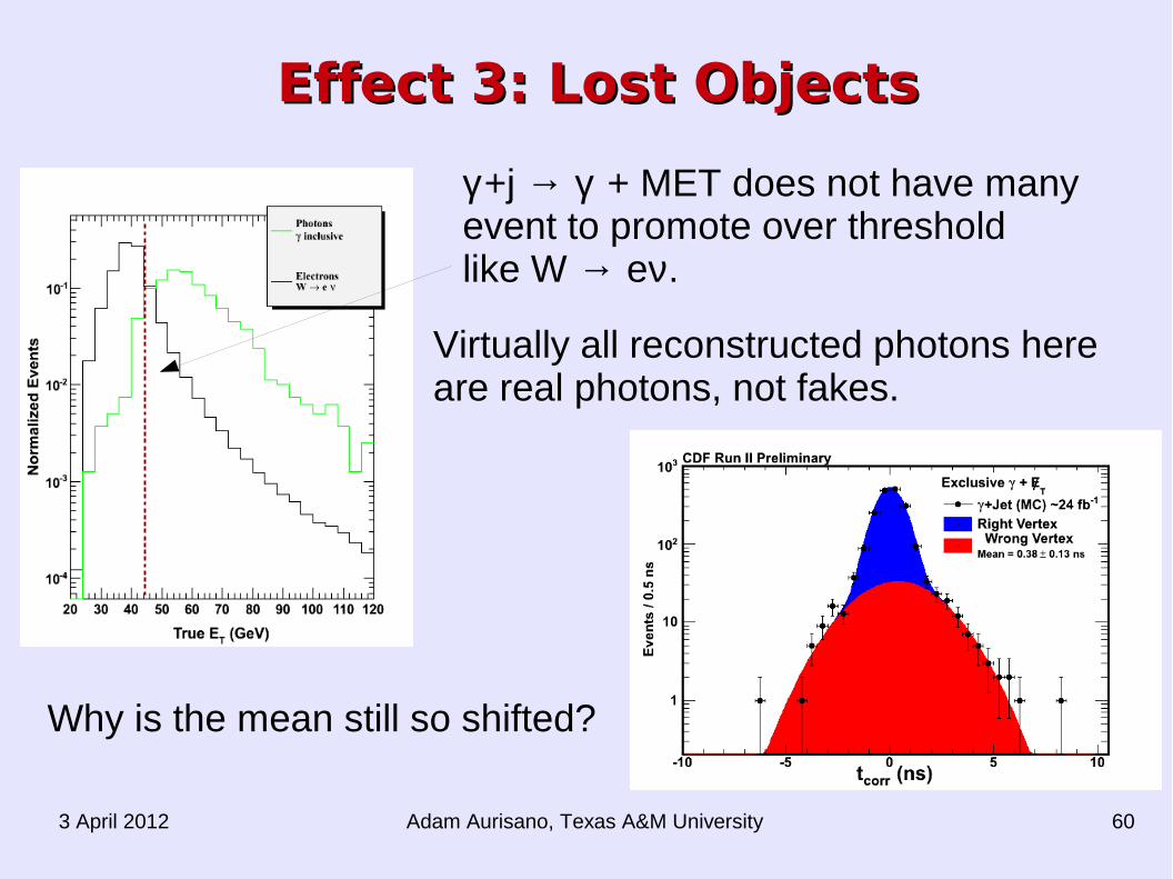
γ +j → γ + MET does not have many event to promote over thresholdlike W → eν.

Virtually all reconstructed photons here are real photons, not fakes.

Why is the mean still so shifted?


Large |Z| VetoLarge |Z| Veto

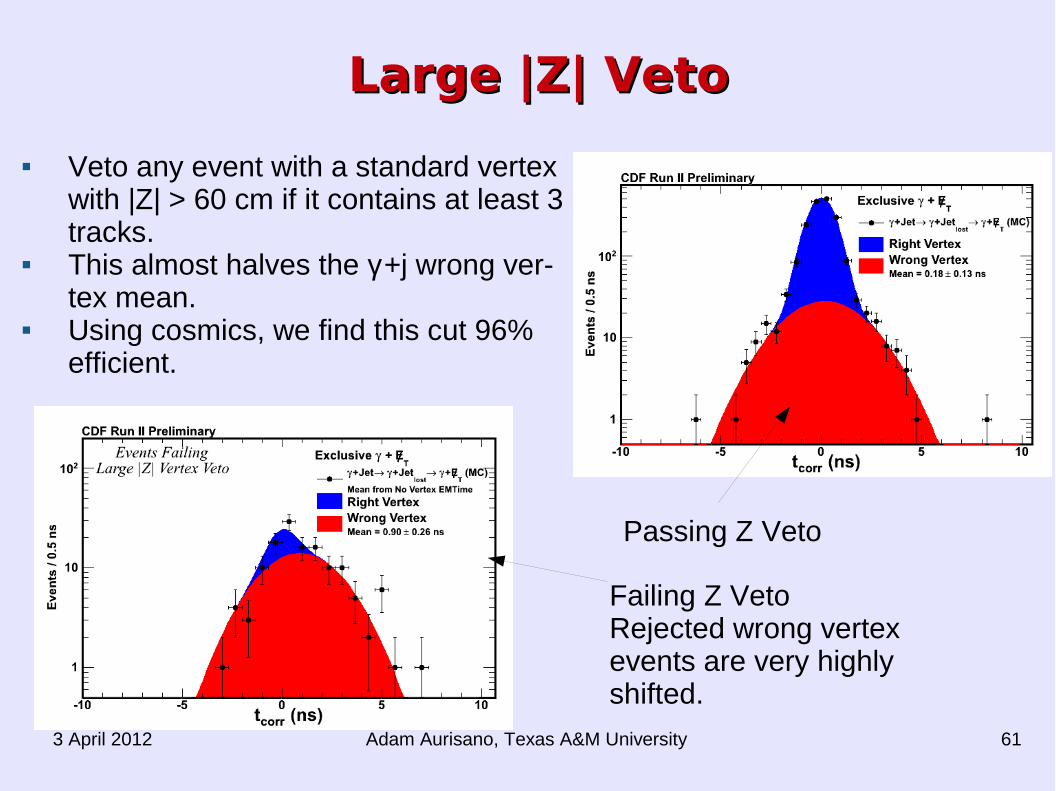
Veto any event with a standard vertex with |Z| > 60 cm if it contains at least 3 tracks.

This almost halves the γ +j wrong ver-tex mean.

Using cosmics, we find this cut 96% efficient.

Passing Z Veto

Failing Z VetoRejected wrong vertexevents are very highlyshifted.


N(SR)/N(CR) vs. Wrong Vertex MeanN(SR)/N(CR) vs. Wrong Vertex Mean

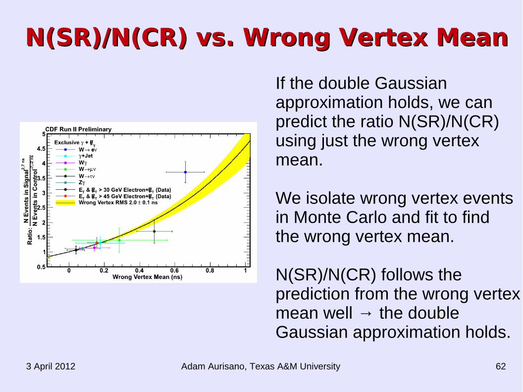
If the double Gaussianapproximation holds, we canpredict the ratio N(SR)/N(CR)using just the wrong vertexmean.

We isolate wrong vertex eventsin Monte Carlo and fit to find the wrong vertex mean.

N(SR)/N(CR) follows the prediction from the wrong vertexmean well → the double Gaussian approximation holds.


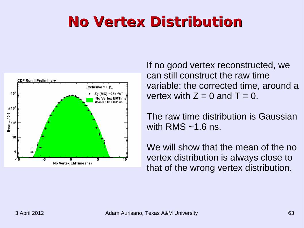
No Vertex DistributionNo Vertex Distribution

If no good vertex reconstructed, we can still construct the raw time variable: the corrected time, around a vertex with Z = 0 and T = 0.

The raw time distribution is Gaussianwith RMS ~1.6 ns.

We will show that the mean of the no vertex distribution is always close to that of the wrong vertex distribution.


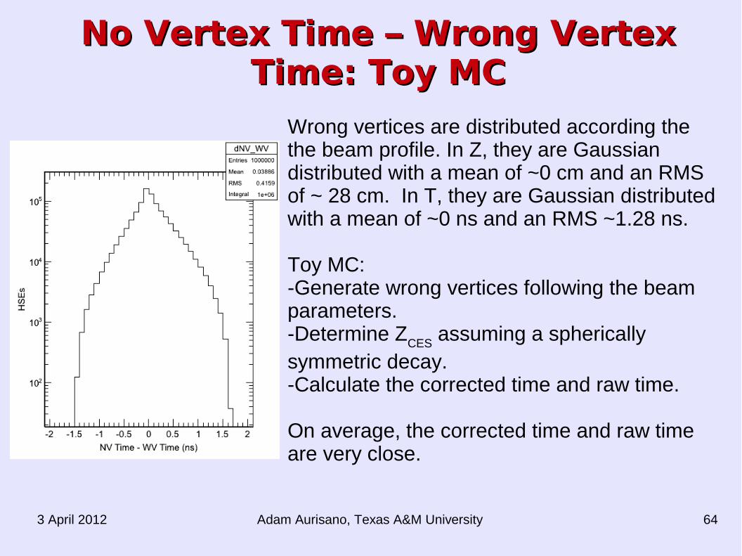
No Vertex Time – Wrong Vertex No Vertex Time – Wrong Vertex Time: Toy MCTime: Toy MC

Wrong vertices are distributed according the the beam profile. In Z, they are Gaussiandistributed with a mean of ~0 cm and an RMS of ~ 28 cm. In T, they are Gaussian distributedwith a mean of ~0 ns and an RMS ~1.28 ns.

Toy MC: -Generate wrong vertices following the beam parameters. -Determine Z

CES assuming a spherically

symmetric decay.-Calculate the corrected time and raw time.

On average, the corrected time and raw time are very close.


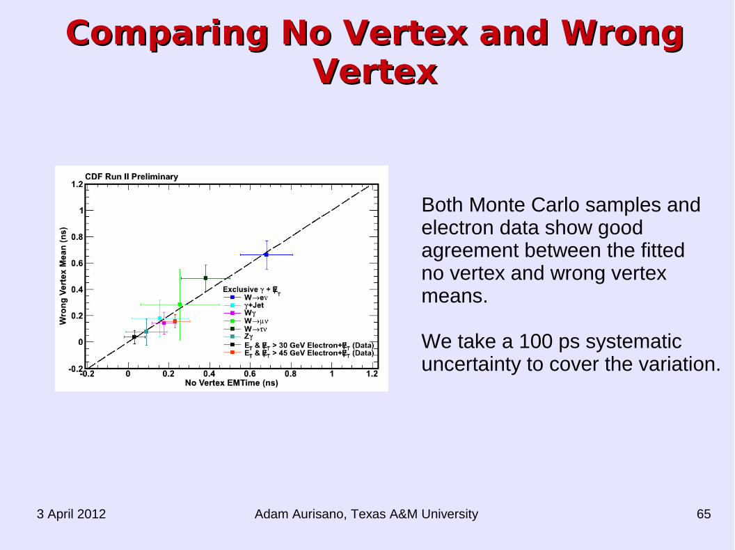
Comparing No Vertex and Wrong Comparing No Vertex and Wrong VertexVertex

Both Monte Carlo samples and electron data show good agreement between the fitted no vertex and wrong vertex means.

We take a 100 ps systematic uncertainty to cover the variation.


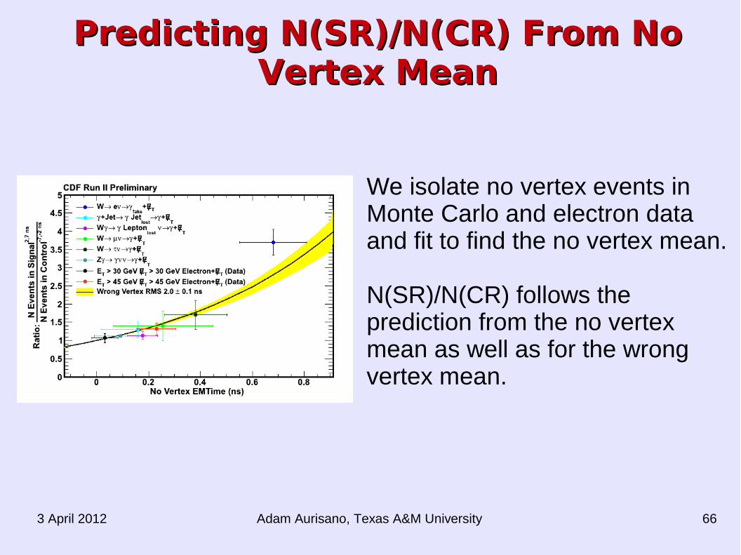
Predicting N(SR)/N(CR) From No Predicting N(SR)/N(CR) From No Vertex MeanVertex Mean

We isolate no vertex events in Monte Carlo and electron dataand fit to find the no vertex mean.

N(SR)/N(CR) follows the prediction from the no vertexmean as well as for the wrong vertex mean.


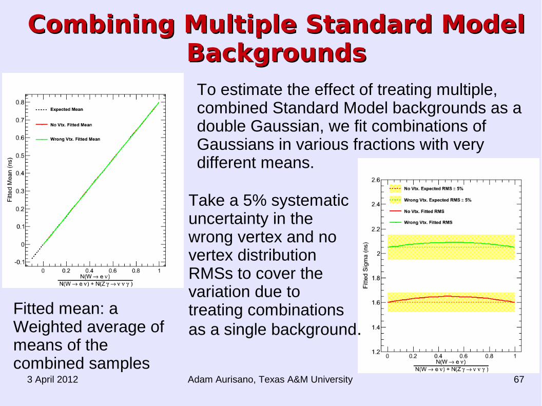
Combining Multiple Standard Model Combining Multiple Standard Model BackgroundsBackgrounds

Fitted mean: a Weighted average of means of thecombined samples

Take a 5% systematic uncertainty in the wrong vertex and no vertex distribution RMSs to cover the variation due to treating combinationsas a single background.

To estimate the effect of treating multiple, combined Standard Model backgrounds as a double Gaussian, we fit combinations of Gaussians in various fractions with very different means.


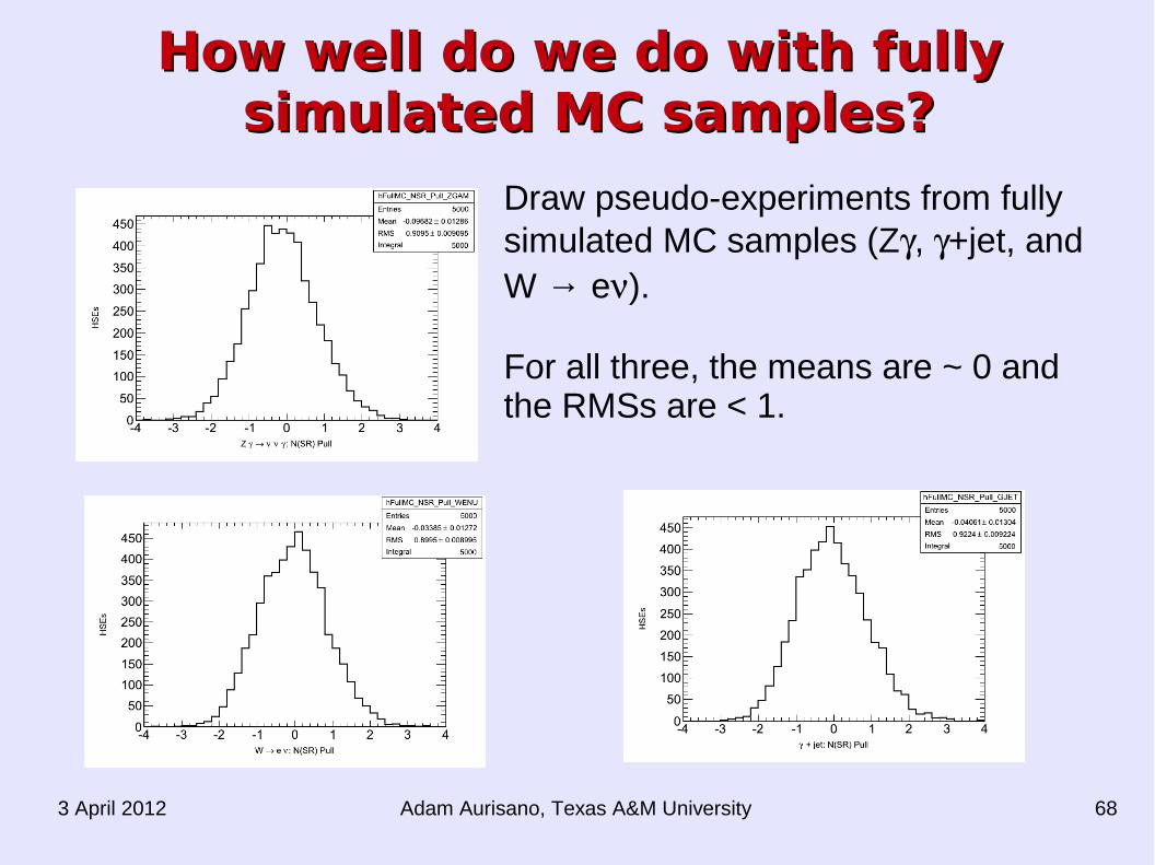
How well do we do with fully How well do we do with fully simulated MC samples?simulated MC samples?

Draw pseudo-experiments from fully simulated MC samples (Z, +jet, and W → e).

For all three, the means are ~ 0 and the RMSs are < 1.


No-Vertex TimeNo-Vertex Time

If no good vertex is reconstructed, we construct the corrected time assuming a vertex with Z = 0 and T = 0. The mean of the no-vertex distribution is always close to that of the wrong-vertex distribution.

Can think of the corrected time having three parts:

1) Geometric time of flight difference relative to the center of the detector (process dependent)

2) Geometric time of flight difference relative to the chosen vertex. This is the same for all processes: it only depends on beam parameters.

3)Time of collision variation for the true collision and a possible wrong vertex is 1.28 ns (from beam profile). Leads to a no-vertex RMS ~ 1.6 ns and a wrong-vertex RMS ~ 2.0 ns.


Estimating Background Estimating Background ContributionsContributions

We have successfully reduced events which tend to produce large wrong vertex mean times.

We still can't count on the wrong vertex mean time being zero. How can we estimate the background contributions in these

circumstances?


Double Gaussian ApproximationDouble Gaussian Approximation

First, we will determine how to estimate the background contribution if there were only one Standard Model background.

Now that the most pathological cases have been removed, Standard Model backgrounds can be described by a double Gaussian

Right vertex: Mean = 0.0 ns, RMS = 0.64 ns Wrong vertex: Mean = ?, RMS = 2.0 ns


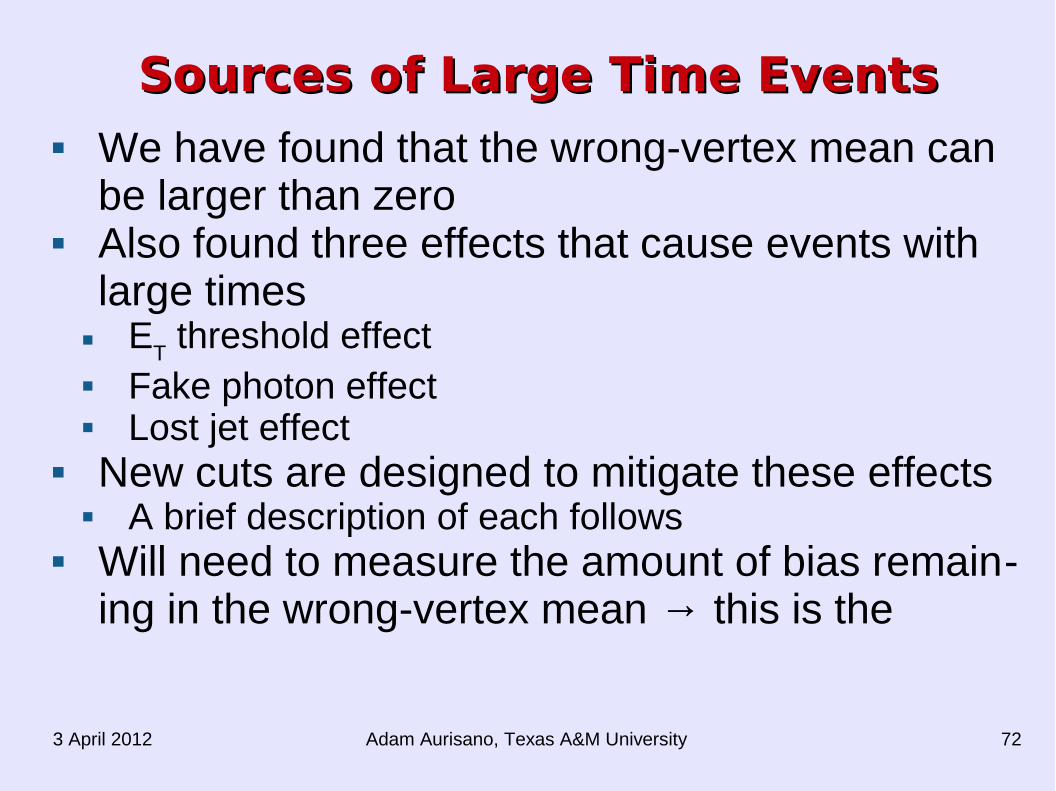
Sources of Large Time EventsSources of Large Time Events We have found that the wrong-vertex mean can

be larger than zero Also found three effects that cause events with

large times E

T threshold effect

Fake photon effect Lost jet effect

New cuts are designed to mitigate these effects A brief description of each follows

Will need to measure the amount of bias remain-ing in the wrong-vertex mean → this is the


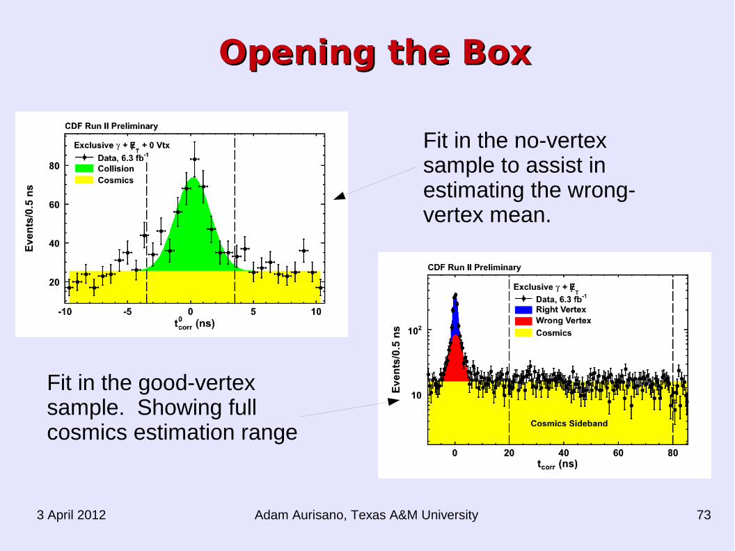
Opening the BoxOpening the Box

Fit in the good-vertex sample. Showing full cosmics estimation range

Fit in the no-vertex sample to assist in estimating the wrong-vertex mean.

Documents

Adam Aurisano - Collider Detector at Fermilabaurisano/aurisano_cornell040312.pdf · 3 April 2012 Adam Aurisano, Texas A&M University 4 Supersymmetry Supersymmetry (SUSY) proposes