AdaGAN: Boosting Generative Models

Ilya Tolstikhin1, Sylvain Gelly2, Olivier Bousquet2, Carl-Johann Simon-Gabriel1, andBernhard Scholkopf1

1Max Planck Institute for Intelligent Systems2Google Brain

Abstract

Generative Adversarial Networks (GAN) [1] are an effective method for training generative models ofcomplex data such as natural images. However, they are notoriously hard to train and can suffer fromthe problem of missing modes where the model is not able to produce examples in certain regions of thespace. We propose an iterative procedure, called AdaGAN, where at every step we add a new componentinto a mixture model by running a GAN algorithm on a reweighted sample. This is inspired by boostingalgorithms, where many potentially weak individual predictors are greedily aggregated to form a strongcomposite predictor. We prove that such an incremental procedure leads to convergence to the truedistribution in a finite number of steps if each step is optimal, and convergence at an exponential rateotherwise. We also illustrate experimentally that this procedure addresses the problem of missing modes.

1 Introduction

Imagine we have a large corpus, containing unlabeled pictures of animals, and our task is to build a generativeprobabilistic model of the data. We run a recently proposed algorithm and end up with a model whichproduces impressive pictures of cats and dogs, but not a single giraffe. A natural way to fix this would beto manually remove all cats and dogs from the training set and run the algorithm on the updated corpus.The algorithm would then have no choice but to produce new animals and, by iterating this process untilthere’s only giraffes left in the training set, we would arrive at a model generating giraffes (assuming sufficientsample size). At the end, we aggregate the models obtained by building a mixture model. Unfortunately, thedescribed meta-algorithm requires manual work for removing certain pictures from the unlabeled trainingset at every iteration.

Let us turn this into an automatic approach, and rather than including or excluding a picture, putcontinuous weights on them. To this end, we train a binary classifier to separate “true” pictures of theoriginal corpus from the set of “synthetic” pictures generated by the mixture of all the models trained sofar. We would expect the classifier to make confident predictions for the true pictures of animals missedby the model (giraffes), because there are no synthetic pictures nearby to be confused with them. Bya similar argument, the classifier should make less confident predictions for the true pictures containinganimals already generated by one of the trained models (cats and dogs). For each picture in the corpus,we can thus use the classifier’s confidence to compute a weight which we use for that picture in the nextiteration, to be performed on the re-weighted dataset.

The present work provides a principled way to perform this re-weighting, with theoretical guaranteesshowing that the resulting mixture models indeed approach the true data distribution.1

Before discussing how to build the mixture, let us consider the question of building a single generativemodel. A recent trend in modelling high dimensional data such as natural images is to use neural net-works [2, 1]. One popular approach are Generative Adversarial Networks (GAN) [1], where the generator

1Note that the term “mixture” should not be interpreted to imply that each component models only one mode: the modelsto be combined into a mixture can themselves cover multiple modes.

1

arX

iv:1

701.

0238

6v2

[st

at.M

L]

24

May

201

7

is trained adversarially against a classifier, which tries to differentiate the true from the generated data.While the original GAN algorithm often produces realistically looking data, several issues were reported inthe literature, among which the missing modes problem, where the generator converges to only one or a fewmodes of the data distribution, thus not providing enough variability in the generated data. This seemsto match the situation described earlier, which is why we will most often illustrate our algorithm with aGAN as the underlying base generator. We call it AdaGAN, for Adaptive GAN, but we could actually useany other generator: a Gaussian mixture model, a VAE [2], a WGAN [3], or even an unrolled [4] or mode-regularized GAN [5], which were both already specifically developed to tackle the missing mode problem.Thus, we do not aim at improving the original GAN or any other generative algorithm. We rather proposeand analyse a meta-algorithm that can be used on top of any of them. This meta-algorithm is similar inspirit to AdaBoost [6] in the sense that each iteration corresponds to learning a “weak” generative model(e.g., GAN) with respect to a re-weighted data distribution. The weights change over time to focus on the“hard” examples, i.e. those that the mixture has not been able to properly generate so far.

1.1 Boosting via Additive Mixtures

Motivated by the problem of missing modes, in this work we propose to use multiple generative modelscombined into a mixture. These generative models are trained iteratively by adding, at each step, anothermodel to the mixture that should hopefully cover the areas of the space not covered by the previous mixturecomponents.2 We show analytically that the optimal next mixture component can be obtained by reweightingthe true data, and thus propose to use the reweighted data distribution as the target for the optimizationof the next mixture components. This leads us naturally to a meta-algorithm, which is similar in spirit toAdaBoost in the sense that each iteration corresponds to learning a “weak” generative model (e.g., GAN)with respect to a reweighted data distribution. The latter adapts over time to focus on the “hard” examples,i.e. those that the mixture has not been able to properly generate thus far.

Before diving into the technical details we provide an informal intuitive discussion of our new meta-algorithm, which we call AdaGAN (a shorthand for Adaptive GAN, similar to AdaBoost). The pseudocodeis presented in Algorithm 1.

On the first step we run the GAN algorithm (or some other generative model) in the usual way andinitialize our generative model with the resulting generator G1. On every t-th step we (a) pick the mixtureweight βt for the next component, (b) update weights Wt of examples from the training set in such a way tobias the next component towards “hard” ones, not covered by the current mixture of generators Gt−1, (c) runthe GAN algorithm, this time importance sampling mini-batches according to the updated weights Wt,resulting in a new generator Gct , and finally (d) update our mixture of generators Gt = (1− βt)Gt−1 + βtG

ct

(notation expressing the mixture of Gt−1 and Gct with probabilities 1−βt and βt). This procedure outputs Tgenerator functions Gc1, . . . , G

cT and T corresponding non-negative weights α1, . . . , αT , which sum to one. For

sampling from the resulting model we first define a generator Gci , by sampling the index i from a multinomialdistribution with parameters α1, . . . , αT , and then we return Gci (Z), where Z ∼ PZ is a standard latent noisevariable used in the GAN literature.

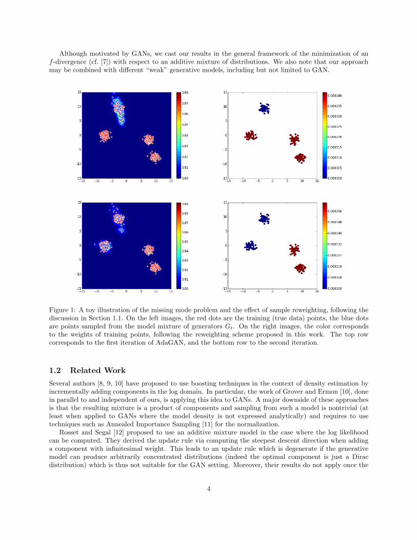
The effect of the described procedure is illustrated in a toy example in Figure 1. On the left images,the red dots are the training (true data) points, the blue dots are points sampled from the model mixtureof generators Gt. The background colour gives the density of the distribution corresponding to Gt, nonzero around the generated points, (almost) zero everywhere else. On the right images, the color correspondsto the weights of training points, following the reweighting scheme proposed in this work. The top rowcorresponds to the first iteration of AdaGAN, and the bottom row to the second iteration. After the firstiteration (the result of the vanilla GAN), we see that only the top left mode is covered, while the threeother modes are not covered at all. The new weights (top right) show that the examples from covered modeare aggressively downweighted. After the second iteration (bottom left), the combined generator can thengenerate two modes.

2Note that the term “mixture” should not be interpreted to imply that each component models only one mode: the modelsto be combined into a mixture can themselves cover multiple modes already.

2

Algorithm 1: AdaGAN, a meta-algorithm to construct a “strong” mixture of T individual GANs,trained sequentially. The mixture weight schedule ChooseMixtureWeight and the training set reweight-ing schedule UpdateTrainingWeights should be provided by the user. Section 3 gives a complete instanceof this family.

Input: Training sample SN := {X1, . . . , XN}.Output: Mixture generative model G = GT .

Train vanilla GAN:

W1 = (1/N, . . . , 1/N)

G1 = GAN(SN ,Wt)

for t = 2, . . . , T do

#Choose a mixture weight for the next component

βt = ChooseMixtureWeight(t)

#Update weights of training examples

Wt = UpdateTrainingWeights(Gt−1, SN , βt)

#Train t-th “weak” component generator Gct

Gct = GAN(SN ,Wt)

#Update the overall generative model

#Notation below means forming a mixture of Gt−1 and Gct .

Gt = (1− βt)Gt−1 + βtGct

end for

3

Although motivated by GANs, we cast our results in the general framework of the minimization of anf -divergence (cf. [7]) with respect to an additive mixture of distributions. We also note that our approachmay be combined with different “weak” generative models, including but not limited to GAN.

Figure 1: A toy illustration of the missing mode problem and the effect of sample reweighting, following thediscussion in Section 1.1. On the left images, the red dots are the training (true data) points, the blue dotsare points sampled from the model mixture of generators Gt. On the right images, the color correspondsto the weights of training points, following the reweighting scheme proposed in this work. The top rowcorresponds to the first iteration of AdaGAN, and the bottom row to the second iteration.

1.2 Related Work

Several authors [8, 9, 10] have proposed to use boosting techniques in the context of density estimation byincrementally adding components in the log domain. In particular, the work of Grover and Ermon [10], donein parallel to and independent of ours, is applying this idea to GANs. A major downside of these approachesis that the resulting mixture is a product of components and sampling from such a model is nontrivial (atleast when applied to GANs where the model density is not expressed analytically) and requires to usetechniques such as Annealed Importance Sampling [11] for the normalization.

Rosset and Segal [12] proposed to use an additive mixture model in the case where the log likelihoodcan be computed. They derived the update rule via computing the steepest descent direction when addinga component with infinitesimal weight. This leads to an update rule which is degenerate if the generativemodel can produce arbitrarily concentrated distributions (indeed the optimal component is just a Diracdistribution) which is thus not suitable for the GAN setting. Moreover, their results do not apply once the

4

weight β becomes non-infinitesimal. In contrast, for any fixed weight of the new component our approachgives the overall optimal update (rather than just the best direction), and applies to any f -divergence.Remarkably, in both theories, improvements of the mixture are guaranteed only if the new “weak” learneris still good enough (see Conditions 14&15)

Similarly, Barron and Li [13] studied the construction of mixtures minimizing the Kullback divergenceand proposed a greedy procedure for doing so. They also proved that under certain conditions, finite mixturescan approximate arbitrary mixtures at a rate 1/k where k is the number of components in the mixture whenthe weight of each newly added component is 1/k. These results are specific to the Kullback divergence butare consistent with our more general results.

Wang et al. [14] propose an additive procedure similar to ours but with a different reweighting scheme,which is not motivated by a theoretical analysis of optimality conditions. On every new iteration the authorspropose to run GAN on the top k training examples with maximum value of the discriminator from the lastiteration. Empirical results of Section 4 show that this heuristic often fails to address the missing modesproblem.

Finally, many papers investigate completely different approaches for addressing the same issue by directlymodifying the training objective of an individual GAN. For instance, Che et al. [5] add an autoencoding costto the training objective of GAN, while Metz et al. [4] allow the generator to “look few steps ahead” whenmaking a gradient step.

The paper is organized as follows. In Section 2 we present our main theoretical results regarding opti-mization of mixture models under general f -divergences. In particular we show that it is possible to buildan optimal mixture in an incremental fashion, where each additional component is obtained by applying aGAN-style procedure with a reweighted distribution. In Section 2.5 we show that if the GAN optimizationat each step is perfect, the process converges to the true data distribution at exponential rate (or evenin a finite number of steps, for which we provide a necessary and sufficient condition). Then we show inSection 2.6 that imperfect GAN solutions still lead to the exponential rate of convergence under certain“weak learnability” conditions. These results naturally lead us to a new boosting-style iterative procedurefor constructing generative models, which is combined with GAN in Section 3, resulting in a new algorithmcalled AdaGAN. Finally, we report initial empirical results in Section 4, where we compare AdaGAN withseveral benchmarks, including original GAN, uniform mixture of multiple independently trained GANs, anditerative procedure of Wang et al. [14].

2 Minimizing f-divergence with Additive Mixtures

In this section we derive a general result on the minimization of f -divergences over mixture models.

2.1 Preliminaries and notations

In this work we will write Pd and Pmodel to denote a real data distribution and our approximate modeldistribution, respectively, both defined over the data space X .

Generative Density Estimation In the generative approach to density estimation, instead of building aprobabilistic model of the data directly, one builds a function G : Z → X that transforms a fixed probabilitydistribution PZ (often called the noise distribution) over a latent space Z into a distribution over X . HencePmodel is the pushforward of PZ , i.e. Pmodel(A) = PZ(G−1(A)). Because of this definition, it is generallyimpossible to compute the density dPmodel(x), hence it is not possible to compute the log-likelihood of thetraining data under the model. However, if PZ is a distribution from which one can sample, it is easy to alsosample from Pmodel (simply sampling from PZ and applying G to each example gives a sample from Pmodel).

So the problem of generative density estimation becomes a problem of finding a function G such thatPmodel looks like Pd in the sense that samples from Pmodel and from Pd look similar. Another way to statethis problem is to say that we are given a measure of similarity between distributions D(Pmodel‖Pd) which

5

can be estimated from samples of those distributions, and thus approximately minimized over a class G offunctions.

f-Divergences In order to measure the agreement between the model distribution and the true distributionof the data we will use an f -divergence defined in the following way:

Df (Q‖P ) :=

∫f

(dQ

dP(x)

)dP (x) (1)

for any pair of distributions P,Q with densities dP , dQ with respect to some dominating reference measure µ.In this work we assume that the function f is convex, defined on (0,∞), and satisfies f(1) = 0. The definitionof Df holds for both continuous and discrete probability measures and does not depend on specific choiceof µ.3 It is easy to verify that Df ≥ 0 and it is equal to 0 when P = Q. Note that Df is not symmetric,but Df (P‖Q) = Df◦(Q‖P ) for f◦(x) := xf(1/x) and any P and Q. The f -divergence is symmetric whenf(x) = f◦(x) for all x ∈ (0,∞), as in this case Df (P,Q) = Df (Q,P ).

We also note that the divergences corresponding to f(x) and f(x) + C · (x − 1) are identical for anyconstant C. In some cases, it is thus convenient to work with f0(x) := f(x) − (x − 1)f ′(1), (where f ′(1) isany subderivative of f at 1) as Df (Q‖P ) = Df0(Q‖P ) for all Q and P , while f0 is nonnegative, nonincreasingon (0, 1], and nondecreasing on (1,∞). In the remainder, we will denote by F the set of functions that aresuitable for f -divergences, i.e. the set of functions of the form f0 for any convex f with f(1) = 0.

Classical examples of f -divergences include the Kullback-Leibler divergence (obtained for f(x) = − log x,f0(x) = − log x + x − 1), the reverse Kullback-Leibler divergence (obtained for f(x) = x log x, f0(x) =x log x− x + 1), the Total Variation distance (f(x) = f0(x) = |x− 1|), and the Jensen-Shannon divergence(f(x) = f0(x) = −(x+ 1) log x+1

2 + x log x). More details can be found in Appendix D. Other examples canbe found in [7]. For further details on f -divergences we refer to Section 1.3 of [15] and [16].

GAN and f-divergences We now explain the connection between the GAN algorithm and f -divergences.The original GAN algorithm [1] consists in optimizing the following criterion:

minG

maxD

EPd[logD(X)] + EPZ

[log(1−D(G(Z)))] , (2)

where D and G are two functions represented by neural networks, and this optimization is actually performedon a pair of samples (one being the training sample, the other one being created from the chosen distribu-tion PZ), which corresponds to approximating the above criterion by using the empirical distributions. For

a fixed G, it has been shown in [1] that the optimal D for (2) is given by D∗(x) = dPd(x)dPd(x)+dPg(x)

and plugging

this optimal value into (2) gives the following:

minG− log(4) + 2JS(Pd ‖Pg) , (3)

where JS is the Jensen-Shannon divergence. Of course, the actual GAN algorithm uses an approximationto D∗ which is computed by training a neural network on a sample, which means that the GAN algorithmcan be considered to minimize an approximation of (3)4. This point of view can be generalized by plugginganother f -divergence into (3), and it turns out that other f -divergences can be written as the solution toa maximization of a criterion similar to (2). Indeed, as demonstrated in [7], any f -divergence between Pdand Pg can be seen as the optimal value of a quantity of the form EPd

[f1(D(X))] + EPg[f2(D(G(Z)))] for

appropriate f1 and f2, and thus can be optimized by the same adversarial training technique.There is thus a strong connection between adversarial training of generative models and minimization of

f -divergences, and this is why we cast the results of this section in the context of general f -divergences.

3The integral in (1) is well defined (but may take infinite values) even if P (dQ = 0) > 0 or Q(dP = 0) > 0. In this case theintegral is understood as Df (Q‖P ) =

∫f(dQ/dP )1[dP (x)>0,dQ(x)>0]dP (x) + f(0)P (dQ = 0) + f◦(0)Q(dP = 0), where both

f(0) and f◦(0) may take value ∞ [15]. This is especially important in case of GAN, where it is impossible to constrain Pmodel

to be absolutely continuous with respect to Pd or vice versa.4Actually the criterion that is minimized is an empirical version of a lower bound of the Jensen-Shannon divergence.

6

Hilbertian Metrics As demonstrated in [17, 18], several commonly used symmetric f -divergences areHilbertian metrics, which in particular means that their square root satisfies the triangle inequality. Thisis true for the Jensen-Shannon divergence5 as well as for the Hellinger distance and the Total Variationamong others. We will denote by FH the set of f functions such that Df is a Hilbertian metric. For those

divergences, we have Df (P‖Q) ≤ (√Df (P‖R) +

√Df (R‖Q))2.

Generative Mixture Models In order to model complex data distributions, it can be convenient to usea mixture model of the following form:

PTmodel :=

T∑i=1

αiPi, (4)

where αi ≥ 0,∑i αi = 1, and each of the T components is a generative density model. This is very natural

in the generative context, since sampling from a mixture corresponds to a two-step sampling, where one firstpicks the mixture component (according to the multinomial distribution whose parameters are the αi) andthen samples from it. Also, this allows to construct complex models from simpler ones.

2.2 Incremental Mixture Building

As discussed earlier, in the context of generative modeling, we are given a measure of similarity betweendistributions. We will restrict ourselves to the case of f -divergences. Indeed, for any f -divergence, itis possible (as explained for example in [7]) to estimate Df (Q ‖P ) from two samples (one from Q, onefrom P ) by training a “discriminator” function, i.e. by solving an optimization problem (which is a binaryclassification problem in the case where the divergence is symmetric6). It turns out that the empiricalestimate D of Df (Q ‖P ) thus obtained provides a criterion for optimizing Q itself. Indeed, D is a functionof Y1, . . . , Yn ∼ Q and X1, . . . , Xn ∼ P , where Yi = G(Zi) for some mapping function G. Hence it is possibleto optimize D with respect to G (and in particular compute gradients with respect to the parameters of Gif G comes from a smoothly parametrized model such as a neural network).

In this work we thus assume that, given an i.i.d. sample from any unknown distribution P we can constructa simple model Q ∈ G which approximately minimizes

minQ∈G

Df (Q ‖P ). (5)

Instead of just modelling the data with a single distribution, we now want to model it with a mixtureof the form (4) where each Pi is obtained by a training procedure of the form (5) with (possibly) differenttarget distributions P for each i.

A natural way to build a mixture is to do it incrementally: we train the first model P1 to minimizeDf (P1 ‖Pd) and set the corresponding weight to α1 = 1, leading to P 1

model = P1. Then after having trainedt components P1, . . . , Pt ∈ G we can form the (t+ 1)-st mixture model by adding a new component Q withweight β as follows:

P t+1model :=

t∑i=1

(1− β)αiPi + βQ. (6)

We are going to choose β ∈ [0, 1] and Q ∈ G greedily, while keeping all the other parameters of the generativemodel fixed, so as to minimize

Df ((1− β)Pg + βQ ‖Pd), (7)

where we denoted Pg := P tmodel the current generative mixture model before adding the new component.We do not necessarily need to find the optimal Q that minimizes (7) at each step. Indeed, it would be

sufficient to find some Q which allows to build a slightly better approximation of Pd. This means that a

5which means such a property can be used in the context of the original GAN algorithm.6One example of such a setting is running GANs, which are known to approximately minimize the Jensen-Shannon divergence.

7

more modest goal could be to find Q such that, for some c < 1,

Df ((1− β)Pg + βQ ‖Pd) ≤ c ·Df (Pg ‖Pd) . (8)

However, we observe that this greedy approach has a significant drawback in practice. Indeed, as webuild up the mixture, we need to make β decrease (as P tmodel approximates Pd better and better, one shouldmake the correction at each step smaller and smaller). Since we are approximating (7) using samples fromboth distributions, this means that the sample from the mixture will only contain a fraction β of examplesfrom Q. So, as t increases, getting meaningful information from a sample so as to tune Q becomes harderand harder (the information is “diluted”).

To address this issue, we propose to optimize an upper bound on (7) which involves a term of theform Df (Q ‖Q0) for some distribution Q0, which can be computed as a reweighting of the original datadistribution Pd.

In the following sections we will analyze the properties of (7) (Section 2.4) and derive upper bounds thatprovide practical optimization criteria for building the mixture (Section 2.3). We will also show that undercertain assumptions, the minimization of the upper bound will lead to the optimum of the original criterion.

This procedure is reminiscent of the AdaBoost algorithm [6], which combines multiple weak predictorsinto one very accurate strong composition. On each step AdaBoost adds one new predictor to the currentcomposition, which is trained to minimize the binary loss on the reweighted training set. The weights areconstantly updated in order to bias the next weak learner towards “hard” examples, which were incorrectlyclassified during previous stages.

2.3 Upper Bounds

Next lemma provides two upper bounds on the divergence of the mixture in terms of the divergence of theadditive component Q with respect to some reference distribution R.

Lemma 1 Let f ∈ F . Given two distributions Pd, Pg and some β ∈ [0, 1], for any distribution Q and anydistribution R such that βdR ≤ dPd, we have

Df ((1− β)Pg + βQ ‖Pd) ≤ βD(Q ‖R) + (1− β)Df

(Pg ‖

Pd − βR1− β

). (9)

If furthermore f ∈ FH , then, for any R, we have

Df ((1− β)Pg + βQ ‖Pd) ≤(√

βDf (Q ‖R) +√Df ((1− β)Pg + βR ‖Pd)

)2

. (10)

Proof For the first inequality, we use the fact that Df is jointly convex. We write Pd = (1−β)Pd−βR1−β +βR

which is a convex combination of two distributions when the assumptions are satisfied.The second inequality follows from using the triangle inequality for the square root of the Hilbertian

metric Df and using convexity of Df in its first argument.

We can exploit the upper bounds of Lemma 1 by introducing some well-chosen distribution R andminimizing with respect to Q. A natural choice for R is a distribution that minimizes the last term of theupper bound (which does not depend on Q).

2.4 Optimal Upper Bounds

In this section we provide general theorems about the optimization of the right-most terms in the upperbounds of Lemma 1.

For the upper bound (10), this means we need to find R minimizing Df ((1− β)Pg + βR ‖Pd). Thesolution for this problem is given in the following theorem.

8

Theorem 1 For any f -divergence Df , with f ∈ F and f differentiable, any fixed distributions Pd, Pg, andany β ∈ (0, 1], the solution to the following minimization problem:

minQ∈P

Df ((1− β)Pg + βQ ‖Pd),

where P is a class of all probability distributions, has the density

dQ∗β(x) =1

β(λ∗dPd(x)− (1− β)dPg(x))+

for some unique λ∗ satisfying∫dQ∗β = 1. Furthermore, β ≤ λ∗ ≤ min(1, β/δ), where δ := Pd(dPg = 0).

Also, λ∗ = 1 if and only if Pd((1− β)dPg > dPd) = 0, which is equivalent to βdQ∗β = dPd − (1− β)dPg.

Proof See Appendix C.1.

Remark 1 The form of Q∗β may look unexpected at first glance: why not setting dQ :=(dPd−(1−β)dPg

)/β,

which would make arguments of the f -divergence identical? Unfortunately, it may be the case that dPd(X) <(1− β)dPg(X) for some of X ∈ X , leading to the negative values of dQ.

For the upper bound (9), we need to minimize Df

(Pg ‖ Pd−βR

1−β

). The solution is given in the next

theorem.

Theorem 2 Given two distributions Pd, Pg and some β ∈ (0, 1], assume

Pd (dPg = 0) < β.

Let f ∈ F . The solution to the minimization problem

minQ:βdQ≤dPd

Df

(Pg ‖

Pd − βQ1− β

)is given by the distribution

dQ†β(x) =1

β

(dPd(x)− λ†(1− β)dPg(x)

)+

for a unique λ† ≥ 1 satisfying∫dQ†β = 1.

Proof See Appendix C.2.

Remark 2 Notice that the term that we optimized in upper bound (10) is exactly the initial objective (7).So that Theorem 1 also tells us what the form of the optimal distribution is for the initial objective.

Remark 3 Surprisingly, in both Theorem 1 and 2, the solution does not depend on the choice of the func-tion f , which means that the solution is the same for any f -divergence. This also means that by replacingf by f◦, we get similar results for the criterion written in the other direction, with again the same solution.Hence the order in which we write the divergence does not matter and the optimal solution is optimal forboth orders.

Remark 4 Note that λ∗ is implicitly defined by a fixed-point equation. In Section 3.1 we will show how itcan be computed efficiently in the case of empirical distributions.

Remark 5 Obviously, λ† ≥ λ∗, where λ∗ was defined in Theorem 1. Moreover, we have λ∗ ≤ 1/λ†. Indeed,

it is enough to insert λ† = 1/λ∗ into definition of Q†β and check that in this case Q†β ≥ 1.

9

2.5 Convergence Analysis for Optimal Updates

In previous section we derived analytical expressions for the distributions R minimizing last terms in upperbounds (9) and (10). Assuming Q can perfectly match R, i.e.Df (Q ‖R) = 0, we are now interested in the

convergence of the mixture (6) to the true data distribution Pd for Q = Q∗β or Q = Q†β .

We start with simple results showing that adding Q∗β or Q†β to the current mixture would yield a strictimprovement of the divergence.

Lemma 2 Under the conditions of Theorem 1, we have

Df

((1− β)Pg + βQ∗β

∥∥Pd) ≤ Df

((1− β)Pg + βPd

∥∥Pd) ≤ (1− β)Df (Pg ‖Pd). (11)

Under the conditions of Theorem 2, we have

Df

(Pg∥∥ Pd − βQ†β

1− β

)≤ Df (Pg ‖Pd) ,

andDf

((1− β)Pg + βQ†β

∥∥Pd) ≤ (1− β)Df (Pg ‖Pd).

Proof The first inequality follows immediately from the optimality of Q∗β (hence the value of the objectiveat Q∗β is smaller than at Pd), and the fact that Df is convex in its first argument and Df (Pd‖Pd) = 0.

The second inequality follows from the optimality of Q†β (hence the value of the objective at Q†β is smallerthan its value at Pd which itself satisfies the condition βdPd ≤ dPd). For the third inequality, we combine

the second inequality with the first inequality of Lemma 1 (with Q = R = Q†β).

The upper bound (11) of Lemma 2 can be refined if the ratio dPg/dPd is almost surely bounded:

Lemma 3 Under the conditions of Theorem 1, if there exists M > 1 such that

Pd((1− β)dPg > MdPd) = 0

then

Df

((1− β)Pg + βQ∗β

∥∥Pd) ≤ f(λ∗) +f(M)(1− λ∗)

M − 1.

Proof We use Inequality (20) of Lemma 6 with X = β, Y = (1 − β)dPg/dPd, and c = λ∗. We easilyverify that X + Y = ((1 − β)dPg + βdPd)/dPd and max(c, Y ) = ((1 − β)dPg + βdQ∗β)/dPd and both haveexpectation 1 with respect to Pd. We thus obtain:

Df ((1− β)Pg + βQ∗β ‖Pd) ≤ f(λ∗) +f(M)− f(λ∗)

M − λ∗(1− λ∗) .

Since λ∗ ≤ 1 and f is non-increasing on (0, 1) we get

Df ((1− β)Pg + βQ∗β ‖Pd) ≤ f(λ∗) +f(M)(1− λ∗)

M − 1.

Remark 6 This upper bound can be tighter than that of Lemma 2 when λ∗ gets close to 1. Indeed, forλ∗ = 1 the upper bound is exactly 0 and is thus tight, while the upper bound of Lemma 2 will not be zero inthis case.

10

Imagine repeatedly adding T new components to the current mixture Pg, where on every step we use thesame weight β and choose the components described in Theorem 1. In this case Lemma 2 guarantees that theoriginal objective value Df (Pg ‖Pd) would be reduced at least to (1−β)TDf (Pg ‖Pd). This exponential rateof convergence, which at first may look surprisingly good, is simply explained by the fact that Q∗β dependson the true distribution Pd, which is of course unknown.

Lemma 2 also suggests setting β as large as possible. This is intuitively clear: the smaller the β, the lesswe alter our current model Pg. As a consequence, choosing small β when Pg is far away from Pd would leadto only minor improvements in objective (7). In fact, the global minimum of (7) can be reached by settingβ = 1 and Q = Pd. Nevertheless, in practice we may prefer to keep β relatively small, preserving what welearned so far through Pg: for instance, when Pg already covered part of the modes of Pd and we want Q tocover the remaining ones. We provide further discussions on choosing β in Section 3.2.

In the reminder of this section we study the convergence of (7) to 0 in the case where we use the upperbound (10) and the weight β is fixed (i.e. the same value at each iteration). This analysis can easily beextended to a variable β.

Lemma 4 For any f ∈ F such that f(x) 6= 0 for x 6= 1, the following conditions are equivalent:

(i) Pd((1− β)dPg > dPd) = 0;

(ii) Df ((1− β)Pg + βQ∗β ‖Pd) = 0.

Proof The first condition is equivalent to λ∗ = 1 according to Theorem 1. In this case, (1−β)Pg+βQ∗β = Pd,hence the divergence is 0. In the other direction, when the divergence is 0, since f is strictly positive for x 6= 1(keep in mind that we can always replace f by f0 to get a non-negative function which will be strictly positiveif f(x) 6= 0 for x 6= 1), this means that with Pd probability 1 we have the equality dPd = (1−β)dPg +βdQ∗β ,

which implies that (1− β)dPg > dPd with Pd probability 1 and also λ∗ = 1.

This result tells that we can not perfectly match Pd by adding a new mixture component to Pg as long asthere are points in the space where our current model Pg severely over-samples. As an example, consider anextreme case where Pg puts a positive mass in a region outside of the support of Pd. Clearly, unless β = 1,we will not be able to match Pd.

Finally, we provide a necessary and sufficient condition for the iterative process to converge to the datadistribution Pd in finite number of steps. The criterion is based on the ratio dP1/dPd, where P1 is the firstcomponent of our mixture model.

Corollary 1 Take any f ∈ F such that f(x) 6= 0 for x 6= 1. Starting from P 1model = P1, update the model

iteratively according to P t+1model = (1 − β)P tmodel + βQ∗β, where on every step Q∗β is as defined in Theorem 1

with Pg := P tmodel. In this case Df (P tmodel ‖Pd) will reach 0 in a finite number of steps if and only if thereexists M > 0 such that

Pd((1− β)dP1 > MdPd) = 0 . (12)

When the finite convergence happens, it takes at most − ln max(M, 1)/ ln(1− β) steps.

Proof From Lemma 4, it is clear that if M ≤ 1 the convergence happens after the first update. So letus assume M > 1. Notice that dP t+1

model = (1 − β)dP tmodel + βdQ∗β = max(λ∗dPd, (1 − β)dP tmodel) so that if

Pd((1 − β)dP tmodel > MdPd) = 0, then Pd((1 − β)dP t+1model > M(1 − β)dPd) = 0. This proves that (12) is a

sufficient condition.Now assume the process converged in a finite number of steps. Let P tmodel be a mixture right before

the final step. Note that P tmodel is represented by (1 − β)t−1P1 + (1 − (1 − β)t−1)P for certain probabilitydistribution P . According to Lemma 4 we have Pd((1 − β)dP tmodel > dPd) = 0. Together these two factsimmediately imply (12).

It is also important to keep in mind that even if (12) is not satisfied the process still converges to the truedistribution at exponential rate (see Lemma 2 as well as Corollaries 2 and 3 below)

11

2.6 Weak to Strong Learnability

In practice the component Q that we add to the mixture is not exactly Q∗β or Q†β , but rather an approximationto them. We need to show that if this approximation is good enough, then we retain the property that (8)is reached. In this section we will show that this is indeed the case.

Looking again at Lemma 1 we notice that the first upper bound is less tight than the second one. Indeed,take the optimal distributions provided by Theorems 1 and 2 and plug them back as R into the upper boundsof Lemma 1. Also assume that Q can match R exactly, i.e. we can achieve Df (Q ‖R) = 0. In this case bothsides of (10) are equal to Df ((1−β)Pg +βQ∗β ‖Pd), which is the optimal value for the original objective (7).On the other hand, (9) does not become an equality and the r.h.s. is not the optimal one for (7).

This means that using (10) allows to reach the optimal value of the original objective (7), whereasusing (9) does not. However, this is not such a big issue since, as we mentioned earlier, we only need toimprove the mixture by adding the next component (we do not need to add the optimal next component).So despite the solution of (7) not being reachable with the first upper bound, we will still show that (8) canbe reached.

The first result provides sufficient conditions for strict improvements when we use the upper bound (9).

Corollary 2 Given two distributions Pd, Pg, and some β ∈ (0, 1], assume

Pd

(dPgdPd

= 0

)< β. (13)

Let Q†β be as defined in Theorem 2. If Q is a distribution satisfying

Df (Q ‖Q†β) ≤ γDf (Pg ‖Pd) (14)

for γ ∈ [0, 1] thenDf ((1− β)Pg + βQ ‖Pd) ≤ (1− β(1− γ))Df (Pg ‖Pd).

Proof Immediately follows from combining Lemma 1, Theorem 1, and Lemma 2.

Next one holds for Hilbertian metrics and corresponds to the upper bound (10).

Corollary 3 Assume f ∈ FH , i.e. Df is a Hilbertian metric. Take any β ∈ (0, 1], Pd, Pg, and let Q∗β beas defined in Theorem 1. If Q is a distribution satisfying

Df (Q ‖Q∗β) ≤ γDf (Pg ‖Pd) (15)

for some γ ∈ [0, 1], then

Df ((1− β)Pg + βQ ‖Pd) ≤(√

γβ +√

1− β)2Df (Pg ‖Pd) .

In particular, the right-hand side is strictly smaller than Df (Pg ‖Pd) as soon as γ < β/4 (and β > 0).

Proof Immediately follows from combining Lemma 1, Theorem 2, and Lemma 2. It is easy to verify thatfor γ < β/4, the coefficient is less than (β/2 +

√1− β)2 which is < 1 (for β > 0).

Remark 7 We emphasize once again that the upper bound (10) and Corollary 3 both hold for Jensen-Shannon, Hellinger, and total variation divergences among others. In particular they can be applied to theoriginal GAN algorithm.

Conditions 14 and 15 may be compared to the “weak learnability” condition of AdaBoost. As long as ourweak learner is able to solve the surrogate problem (5) of matching respectively Q†β or Q∗β accurately enough,the original objective (7) is guaranteed to decrease as well. It should be however noted that Condition 15

12

with γ < β/4 is perhaps too strong to call it “weak learnability”. Indeed, as already mentioned before,the weight β is expected to decrease to zero as the number of components in the mixture distribution Pgincreases. This leads to γ → 0, making it harder to meet Condition 15. This obstacle may be partiallyresolved by the fact that we will use a GAN to fit Q, which corresponds to a relatively rich7 class of modelsG in (5). In other words, our weak learner is not so weak.

On the other hand, Condition (14) of Corollary 2 is much milder. No matter what γ ∈ [0, 1] and β ∈ (0, 1]we choose, the new component Q is guaranteed to strictly improve the objective functional. This comes atthe price of the additional Condition (13), which asserts that β should be larger than the mass of true dataPd missed by the current model Pg. We argue that this is a rather reasonable condition: if Pg misses manymodes of Pd we would prefer assigning a relatively large weight β to the new component Q.

3 AdaGAN

In this section we provide a more detailed description of Algorithm 1 from Section 1.1, in particular how toreweight the training examples for the next iteration and how to choose the mixture weights.

In a nutshell, at each iteration we want to add a new component Q to the current mixture Pg withweight β, to create a mixture with distribution (1 − β)Pg + βQ. This component Q should approach an“optimal target” Q∗β and we know from Theorem 1 that:

dQ∗β =dPdβ

(λ∗ − (1− β)

dPgdPd

)+

.

Computing this distribution requires to know the density ratio dPg/dPd, which is not directly accessible,but it can be estimated using the idea of adversarial training. Indeed, we can train a discriminator D todistinguish between samples from Pd and Pg. It is known that for an arbitrary f -divergence, there existsa corresponding function h (see [7]) such that the values of the optimal discriminator D are related to thedensity ratio in the following way:

dPgdPd

(X) = h(D(X)

). (16)

In particular, for the Jensen-Shannon divergence, used by the original GAN algorithm, it holds that h(D(X)

)=

1−D(X)D(X) . So in this case for the optimal discriminator we have

dQ∗β =dPdβ

(λ∗ − (1− β)h(D)

)+,

which can be viewed as a reweighted version of the original data distribution Pd.In particular, when we compute dQ∗β on the training sample SN = (X1, . . . , XN ), each example Xi has

the following weight:

wi =piβ

(λ∗ − (1− β)h(di)

)+

(17)

with pi = dPd(Xi) and di = D(Xi). In practice, we use the empirical distribution over the training samplewhich means we set pi = 1/N .

3.1 How to compute λ∗ of Theorem 1

Next we derive an algorithm to determine λ∗. We need to find a value of λ∗ such that the weights wi in (17)are normalized, i.e.: ∑

i

wi =∑

i∈I(λ∗)

piβ

(λ∗ − (1− β)h(di)

)= 1 ,

7The hardness of meeting Condition 15 of course largely depends on the class of models G used to fit Q in (5). For now weignore this question and leave it for future research.

13

where I(λ) := {i : λ > (1− β)h(di)}. This in turn yields:

λ∗ =β∑

i∈I(λ∗) pi

1 +(1− β)

β

∑i∈I(λ∗)

pih(di)

. (18)

Now, to compute the r.h.s., we need to know I(λ∗). To do so, we sort the values h(di) in increasing order:h(d1) ≤ h(d2) ≤ . . . ≤ h(dN ). Then I(λ∗) is simply a set consisting of the first k values, where we have todetermine k. Thus, it suffices to test successively all positive integers k until the λ given by Equation (18)verifies:

(1− β)h(dk) < λ ≤ (1− β)h(dk+1) .

This procedure is guaranteed to converge, because by Theorem 1, we know that λ∗ exists, and it satisfies (18).In summary, λ∗ can be determined by Algorithm 2.

Algorithm 2: Determining λ∗

1 Sort the values h(di) in increasing order ;

2 Initialize λ← βp1

(1 + 1−β

β p1h(d1))

and k ← 1 ;

3 while (1− β)h(dk) ≥ λ do4 k ← k + 1;

5 λ← β∑ki=1 pi

(1 + (1−β)

β

∑ki=1 pih(di)

)

3.2 How to choose a mixture weight β

While for every β there is an optimal reweighting scheme, the weights from (17) depend on β. In particular,if β is large enough to verify dPd(x)λ∗ − (1 − β)dPg(x) ≥ 0 for all x, the optimal component Q∗β satisfies(1 − β)Pg + βQ∗β = Pd, as proved in Lemma 4. In other words, in this case we exactly match the datadistribution Pd, assuming the GAN can approximate the target Q∗β perfectly. This criterion alone wouldlead to choosing β = 1. However in practice we know we can’t get a generator that produces exactly thetarget distribution Q∗β . We thus propose a few heuristics one can follow to choose β:

– Any fixed constant value β for all iterations.

– All generators to be combined with equal weights in the final mixture model. This corresponds tosetting βt = 1

t , where t is the iteration.

– Instead of choosing directly a value for β one could pick a ratio 0 < r < 1 of examples which shouldhave a weight wi > 0. Given such an r, there is a unique value of β (βr) resulting in wi > 0 for exactlyN · r training examples. Such a value βr can be determined by binary search over β in Algorithm 2.Possible choices for r include:

– r constant, chosen experimentally.

– r decreasing with the number of iterations, e.g., r = c1e−c2t for any positive constants c1, c2.

– Alternatively, one can set a particular threshold for the density ratio estimate h(D), compute thefraction r of training examples that have a value above that threshold and derive β from this ratior (as above). Indeed, when h(D) is large, that means that the generator does not generate enoughexamples in that region, and the next iteration should be encouraged to generate more there.

14

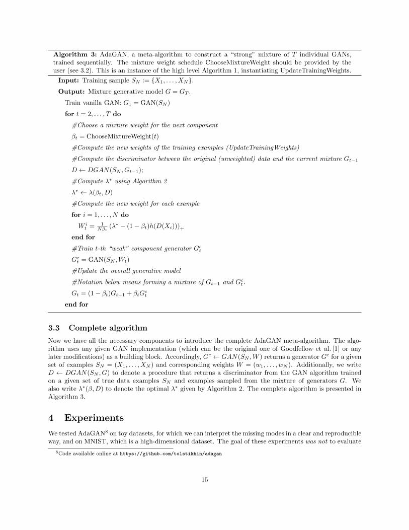
Algorithm 3: AdaGAN, a meta-algorithm to construct a “strong” mixture of T individual GANs,trained sequentially. The mixture weight schedule ChooseMixtureWeight should be provided by theuser (see 3.2). This is an instance of the high level Algorithm 1, instantiating UpdateTrainingWeights.

Input: Training sample SN := {X1, . . . , XN}.Output: Mixture generative model G = GT .

Train vanilla GAN: G1 = GAN(SN )

for t = 2, . . . , T do

#Choose a mixture weight for the next component

βt = ChooseMixtureWeight(t)

#Compute the new weights of the training examples (UpdateTrainingWeights)

#Compute the discriminator between the original (unweighted) data and the current mixture Gt−1

D ← DGAN(SN , Gt−1);

#Compute λ∗ using Algorithm 2

λ∗ ← λ(βt, D)

#Compute the new weight for each example

for i = 1, . . . , N do

W it = 1

Nβt(λ∗ − (1− βt)h(D(Xi)))+

end for

#Train t-th “weak” component generator Gct

Gct = GAN(SN ,Wt)

#Update the overall generative model

#Notation below means forming a mixture of Gt−1 and Gct .

Gt = (1− βt)Gt−1 + βtGct

end for

3.3 Complete algorithm

Now we have all the necessary components to introduce the complete AdaGAN meta-algorithm. The algo-rithm uses any given GAN implementation (which can be the original one of Goodfellow et al. [1] or anylater modifications) as a building block. Accordingly, Gc ← GAN(SN ,W ) returns a generator Gc for a givenset of examples SN = (X1, . . . , XN ) and corresponding weights W = (w1, . . . , wN ). Additionally, we writeD ← DGAN(SN , G) to denote a procedure that returns a discriminator from the GAN algorithm trainedon a given set of true data examples SN and examples sampled from the mixture of generators G. Wealso write λ∗(β,D) to denote the optimal λ∗ given by Algorithm 2. The complete algorithm is presented inAlgorithm 3.

4 Experiments

We tested AdaGAN8 on toy datasets, for which we can interpret the missing modes in a clear and reproducibleway, and on MNIST, which is a high-dimensional dataset. The goal of these experiments was not to evaluate

8Code available online at https://github.com/tolstikhin/adagan

15

the visual quality of individual sample points, but to demonstrate that the re-weighting scheme of AdaGANpromotes diversity and effectively covers the missing modes.

4.1 Toy datasets

The target distribution is defined as a mixture of normal distributions, with different variances. The distancesbetween the means are relatively large compared to the variances, so that each Gaussian of the mixture is“isolated”. We vary the number of modes to test how well each algorithm performs when there are fewer ormore expected modes.

More precisely, we set X = R2, each Gaussian component is isotropic, and their centers are sampleduniformly in a square. That particular random seed is fixed for all experiments, which means that for agiven number of modes, the target distribution is always the same. The variance parameter is the same foreach component, and is decreasing with the number of modes, so that the modes stay apart from each other.

This target density is very easy to learn, using a mixture of Gaussians model, and for example the EMalgorithm [19]. If applied to the situation where the generator is producing single Gaussians (i.e. PZ is astandard Gaussian and G is a linear function), then AdaGAN produces a mixture of Gaussians, however itdoes so incrementally unlike EM, which keeps a fixed number of components. In any way AdaGAN was nottailored for this particular case and we use the Gaussian mixture model simply as a toy example to illustratethe missing modes problem.

4.1.1 Algorithms

We compare different meta-algorithms based on GAN, and the baseline GAN algorithm. All the meta-algorithms use the same implementation of the underlying GAN procedure. In all cases, the generatoruses latent space Z = R5, and two ReLU hidden layers, of size 10 and 5 respectively. The correspondingdiscriminator has two ReLU hidden layers of size 20 and 10 respectively. We use 64k training examples, and15 epochs, which is enough compared to the small scale of the problem, and all networks converge properlyand overfitting is never an issue. Despite the simplicity of the problem, there are already differences betweenthe different approaches.

We compare the following algorithms:

– The baseline GAN algorithm, called Vanilla GAN in the results.

– The best model out of T runs of GAN, that is: run T GAN instances independently, then take the runthat performs best on a validation set. This gives an additional baseline with similar computationalcomplexity as the ensemble approaches. Note that the selection of the best run is done on the reportedtarget metric (see below), rather than on the internal metric. As a result this baseline is slightlyoverestimated. This procedure is called Best of T in the results.

– A mixture of T GAN generators, trained independently, and combined with equal weights (the “bag-ging” approach). This procedure is called Ensemble in the results.

– A mixture of GAN generators, trained sequentially with different choices of data reweighting:

– The AdaGAN algorithm (Algorithm 1), for β = 1/t, i.e. each component will have the sameweight in the resulting mixture (see § 3.2). This procedure is called Boosted in the results.

– The AdaGAN algorithm (Algorithm 1), for a constant β, exploring several values. This procedureis called for example Beta0.3 for β = 0.3 in the results.

– Reweighting similar to “Cascade GAN” from [14], i.e. keeping the top r fraction of examples,based on the discriminator corresponding to the previous generator. This procedure is called forexample TopKLast0.3 for r = 0.3.

– Keep the top r fraction of examples, based on the discriminator corresponding to the mixture ofall previous generators. This procedure is called for example TopK0.3 for r = 0.3.

16

4.1.2 Metrics

To evaluate how well the generated distribution matches the target distribution, we use a coverage metric C.We compute the probability mass of the true data “covered” by the model distribution Pmodel. Moreprecisely, we compute C := Pd(dPmodel > t) with t such that Pmodel(dPmodel > t) = 0.95. This metricis more interpretable than the likelihood, making it easier to assess the difference in performance of thealgorithms. To approximate the density of Pmodel we use a kernel density estimation method, where thebandwidth is chosen by cross validation. Note that we could also use the discriminator D to approximatethe coverage as well, using the relation from (16).

Another metric is the likelihood of the true data under the generated distribution. More precisely, wecompute L := 1

N

∑i logPmodel(xi), on a sample of N examples from the data. Note that [20] proposes a

more general and elegant approach (but less straightforward to implement) to have an objective measure ofGAN. On the simple problems we tackle here, we can precisely estimate the likelihood.

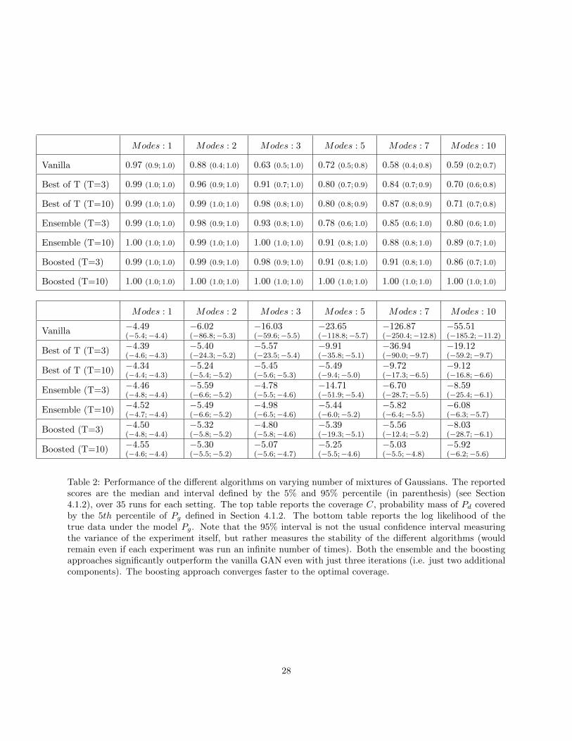
In the main results we report the metric C and in Appendix E we report both L and C. For a givenmetric, we repeat the run 35 times with the same parameters (but different random seeds). For each run, thelearning rate is optimized using a grid search on a validation set. We report the median over those multipleruns, and the interval corresponding to the 5% and 95% percentiles. Note this is not a confidence interval ofthe median, which would shrink to a singleton with an infinite number of runs. Instead, this gives a measureof the stability of each algorithm. The optimizer is a simple SGD: Adam was also tried but gave slightly lessstable results.

4.1.3 Results

With the vanilla GAN algorithm, we observe that not all the modes are covered (see Figure 1 for anillustration). Different modes (and even different number of modes) are possibly covered at each restart ofthe algorithm, so restarting the algorithm with different random seeds and taking the best (“best of T”) canimprove the results.

Figure 3 summarizes the performance of the main algorithms on the C metric, as a function of the numberof iterations T . Table 1 gives more detailed results, varying the number of modes for the target distribution.Appendix E contains details on variants for the reweighting heuristics as well as results for the L metric.

As expected, both the ensemble and the boosting approaches significantly outperform the vanilla GANand the “best of T” algorithm. Interestingly, the improvements are significant even after just one or twoadditional iterations (T = 2 or T = 3). The boosted approach converges much faster. In addition, thevariance is much lower, improving the likelihood that a given run gives good results. On this setup, thevanilla GAN approach has a significant number of catastrophic failures (visible in the lower bound of theinterval).

Empirical results on combining AdaGAN meta-algorithm with the unrolled GANs [4] are available inAppendix A.

4.2 MNIST and MNIST3

We ran experiments both on the original MNIST and on the 3-digit MNIST (MNIST3) [5, 4] dataset,obtained by concatenating 3 randomly chosen MNIST images to form a 3-digit number between 0 and 999.According to [5, 4], MNIST contains 10 modes, while MNIST3 contains 1000 modes, and these modes canbe detected using the pre-trained MNIST classifier. We combined AdaGAN both with simple MLP GANsand DCGANs [21]. We used T ∈ {5, 10}, tried models of various sizes and performed a reasonable amountof hyperparameter search. For the details we refer to Appendix B.

Similarly to [4, Sec 3.3.1] we failed to reproduce the missing modes problem for MNIST3 reported in[5] and found that simple GAN architectures are capable of generating all 1000 numbers. The authorsof [4] proposed to artificially introduce the missing modes again by limiting the generators’ flexibility. Inour experiments, GANs trained with the architectures reported in [4] were often generating poorly lookingdigits. As a result, the pre-trained MNIST classifier was outputting random labels, which again led to full

17

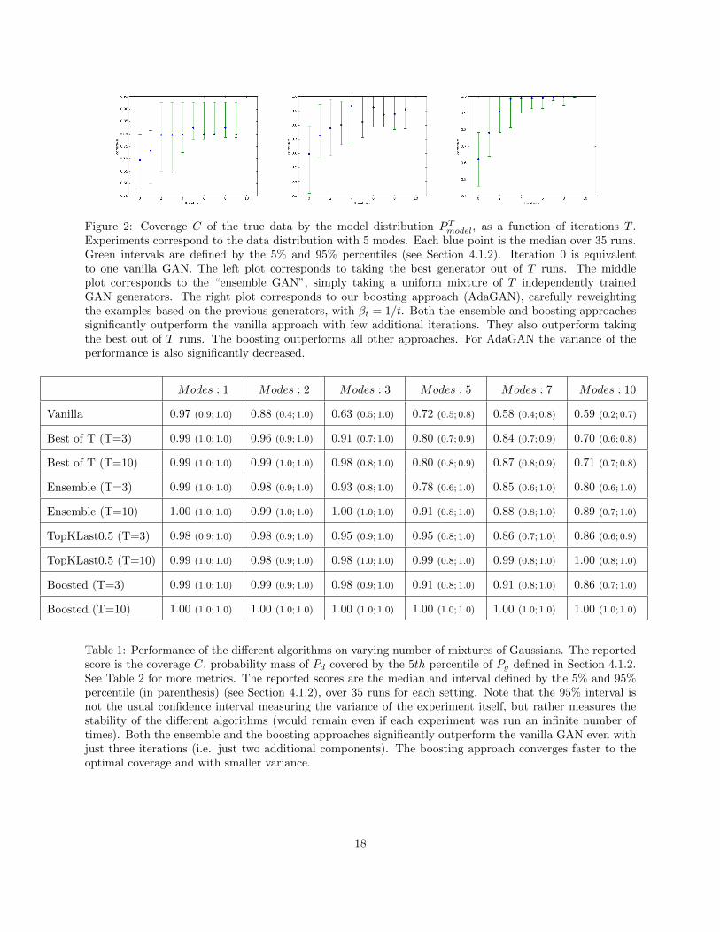
Figure 2: Coverage C of the true data by the model distribution PTmodel, as a function of iterations T .Experiments correspond to the data distribution with 5 modes. Each blue point is the median over 35 runs.Green intervals are defined by the 5% and 95% percentiles (see Section 4.1.2). Iteration 0 is equivalentto one vanilla GAN. The left plot corresponds to taking the best generator out of T runs. The middleplot corresponds to the “ensemble GAN”, simply taking a uniform mixture of T independently trainedGAN generators. The right plot corresponds to our boosting approach (AdaGAN), carefully reweightingthe examples based on the previous generators, with βt = 1/t. Both the ensemble and boosting approachessignificantly outperform the vanilla approach with few additional iterations. They also outperform takingthe best out of T runs. The boosting outperforms all other approaches. For AdaGAN the variance of theperformance is also significantly decreased.

Modes : 1 Modes : 2 Modes : 3 Modes : 5 Modes : 7 Modes : 10

Vanilla 0.97 (0.9; 1.0) 0.88 (0.4; 1.0) 0.63 (0.5; 1.0) 0.72 (0.5; 0.8) 0.58 (0.4; 0.8) 0.59 (0.2; 0.7)

Best of T (T=3) 0.99 (1.0; 1.0) 0.96 (0.9; 1.0) 0.91 (0.7; 1.0) 0.80 (0.7; 0.9) 0.84 (0.7; 0.9) 0.70 (0.6; 0.8)

Best of T (T=10) 0.99 (1.0; 1.0) 0.99 (1.0; 1.0) 0.98 (0.8; 1.0) 0.80 (0.8; 0.9) 0.87 (0.8; 0.9) 0.71 (0.7; 0.8)

Ensemble (T=3) 0.99 (1.0; 1.0) 0.98 (0.9; 1.0) 0.93 (0.8; 1.0) 0.78 (0.6; 1.0) 0.85 (0.6; 1.0) 0.80 (0.6; 1.0)

Ensemble (T=10) 1.00 (1.0; 1.0) 0.99 (1.0; 1.0) 1.00 (1.0; 1.0) 0.91 (0.8; 1.0) 0.88 (0.8; 1.0) 0.89 (0.7; 1.0)

TopKLast0.5 (T=3) 0.98 (0.9; 1.0) 0.98 (0.9; 1.0) 0.95 (0.9; 1.0) 0.95 (0.8; 1.0) 0.86 (0.7; 1.0) 0.86 (0.6; 0.9)

TopKLast0.5 (T=10) 0.99 (1.0; 1.0) 0.98 (0.9; 1.0) 0.98 (1.0; 1.0) 0.99 (0.8; 1.0) 0.99 (0.8; 1.0) 1.00 (0.8; 1.0)

Boosted (T=3) 0.99 (1.0; 1.0) 0.99 (0.9; 1.0) 0.98 (0.9; 1.0) 0.91 (0.8; 1.0) 0.91 (0.8; 1.0) 0.86 (0.7; 1.0)

Boosted (T=10) 1.00 (1.0; 1.0) 1.00 (1.0; 1.0) 1.00 (1.0; 1.0) 1.00 (1.0; 1.0) 1.00 (1.0; 1.0) 1.00 (1.0; 1.0)

Table 1: Performance of the different algorithms on varying number of mixtures of Gaussians. The reportedscore is the coverage C, probability mass of Pd covered by the 5th percentile of Pg defined in Section 4.1.2.See Table 2 for more metrics. The reported scores are the median and interval defined by the 5% and 95%percentile (in parenthesis) (see Section 4.1.2), over 35 runs for each setting. Note that the 95% interval isnot the usual confidence interval measuring the variance of the experiment itself, but rather measures thestability of the different algorithms (would remain even if each experiment was run an infinite number oftimes). Both the ensemble and the boosting approaches significantly outperform the vanilla GAN even withjust three iterations (i.e. just two additional components). The boosting approach converges faster to theoptimal coverage and with smaller variance.

18

coverage of the 1000 numbers. We tried to threshold the confidence of the pre-trained classifier, but decidedthat this metric was too ad-hoc.

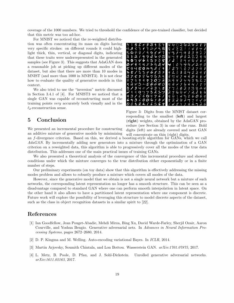
Figure 3: Digits from the MNIST dataset cor-responding to the smallest (left) and largest(right) weights, obtained by the AdaGAN pro-cedure (see Section 3) in one of the runs. Bolddigits (left) are already covered and next GANwill concentrate on thin (right) digits.

For MNIST we noticed that the re-weighted distribu-tion was often concentrating its mass on digits havingvery specific strokes: on different rounds it could high-light thick, thin, vertical, or diagonal digits, indicatingthat these traits were underrepresented in the generatedsamples (see Figure 3). This suggests that AdaGAN doesa reasonable job at picking up different modes of thedataset, but also that there are more than 10 modes inMNIST (and more than 1000 in MNIST3). It is not clearhow to evaluate the quality of generative models in thiscontext.

We also tried to use the “inversion” metric discussedin Section 3.4.1 of [4]. For MNIST3 we noticed that asingle GAN was capable of reconstructing most of thetraining points very accurately both visually and in the`2-reconstruction sense.

5 Conclusion

We presented an incremental procedure for constructingan additive mixture of generative models by minimizingan f -divergence criterion. Based on this, we derived a boosting-style algorithm for GANs, which we callAdaGAN. By incrementally adding new generators into a mixture through the optimization of a GANcriterion on a reweighted data, this algorithm is able to progressively cover all the modes of the true datadistribution. This addresses one of the main practical issues of training GANs.

We also presented a theoretical analysis of the convergence of this incremental procedure and showedconditions under which the mixture converges to the true distribution either exponentially or in a finitenumber of steps.

Our preliminary experiments (on toy data) show that this algorithm is effectively addressing the missingmodes problem and allows to robustly produce a mixture which covers all modes of the data.

However, since the generative model that we obtain is not a single neural network but a mixture of suchnetworks, the corresponding latent representation no longer has a smooth structure. This can be seen as adisadvantage compared to standard GAN where one can perform smooth interpolation in latent space. Onthe other hand it also allows to have a partitioned latent representation where one component is discrete.Future work will explore the possibility of leveraging this structure to model discrete aspects of the dataset,such as the class in object recognition datasets in a similar spirit to [22].

References

[1] Ian Goodfellow, Jean Pouget-Abadie, Mehdi Mirza, Bing Xu, David Warde-Farley, Sherjil Ozair, AaronCourville, and Yoshua Bengio. Generative adversarial nets. In Advances in Neural Information Pro-cessing Systems, pages 2672–2680, 2014.

[2] D. P. Kingma and M. Welling. Auto-encoding variational Bayes. In ICLR, 2014.

[3] Martin Arjovsky, Soumith Chintala, and Lon Bottou. Wasserstein GAN. arXiv:1701.07875, 2017.

[4] L. Metz, B. Poole, D. Pfau, and J. Sohl-Dickstein. Unrolled generative adversarial networks.arXiv:1611.02163, 2017.

19

[5] Tong Che, Yanran Li, Athul Paul Jacob, Yoshua Bengio, and Wenjie Li. Mode regularized generativeadversarial networks. arXiv:1612.02136, 2016.

[6] Y. Freund and R. E. Schapire. A decision-theoretic generalization of on-line learning and an applicationto boosting. Journal of Computer and System Sciences, 55(1):119–139, 1997.

[7] Sebastian Nowozin, Botond Cseke, and Ryota Tomioka. f-GAN: Training generative neural samplersusing variational divergence minimization. In Advances in Neural Information Processing Systems, 2016.

[8] Max Welling, Richard S. Zemel, and Geoffrey E. Hinton. Self supervised boosting. In Advances inneural information processing systems, pages 665–672, 2002.

[9] Zhuowen Tu. Learning generative models via discriminative approaches. In 2007 IEEE Conference onComputer Vision and Pattern Recognition, pages 1–8. IEEE, 2007.

[10] Aditya Grover and Stefano Ermon. Boosted generative models. ICLR 2017 conference submission, 2016.

[11] R. M. Neal. Annealed importance sampling. Statistics and Computing, 11(2):125–139, 2001.

[12] Saharon Rosset and Eran Segal. Boosting density estimation. In Advances in Neural InformationProcessing Systems, pages 641–648, 2002.

[13] A Barron and J Li. Mixture density estimation. Biometrics, 53:603–618, 1997.

[14] Yaxing Wang, Lichao Zhang, and Joost van de Weijer. Ensembles of generative adversarial networks.arXiv:1612.00991, 2016.

[15] F. Liese and K.-J. Miescke. Statistical Decision Theory. Springer, 2008.

[16] M. D. Reid and R. C. Williamson. Information, divergence and risk for binary experiments. Journal ofMachine Learning Research, 12:731–817, 2011.

[17] Bent Fuglede and Flemming Topsoe. Jensen-shannon divergence and hilbert space embedding. In IEEEInternational Symposium on Information Theory, pages 31–31, 2004.

[18] Matthias Hein and Olivier Bousquet. Hilbertian metrics and positive definite kernels on probabilitymeasures. In AISTATS, pages 136–143, 2005.

[19] A. P. Dempster, N. M. Laird, and D. B. Rubin. Maximum likelihood from incomplete data via the EMalgorithm. Journal of the Royal Statistical Society, B, 39:1–38, 1977.

[20] Yuhuai Wu, Yuri Burda, Ruslan Salakhutdinov, and Roger Grosse. On the quantitative analysis ofdecoder-based generative models, 2016.

[21] A. Radford, L. Metz, and S. Chintala. Unsupervised representation learning with deep convolutionalgenerative adversarial networks. In ICLR, 2016.

[22] Xi Chen, Yan Duan, Rein Houthooft, John Schulman, Ilya Sutskever, and Pieter Abbeel. Infogan: In-terpretable representation learning by information maximizing generative adversarial nets. In Advancesin Neural Information Processing Systems, pages 2172–2180, 2016.

20

A Further details on toy experiments

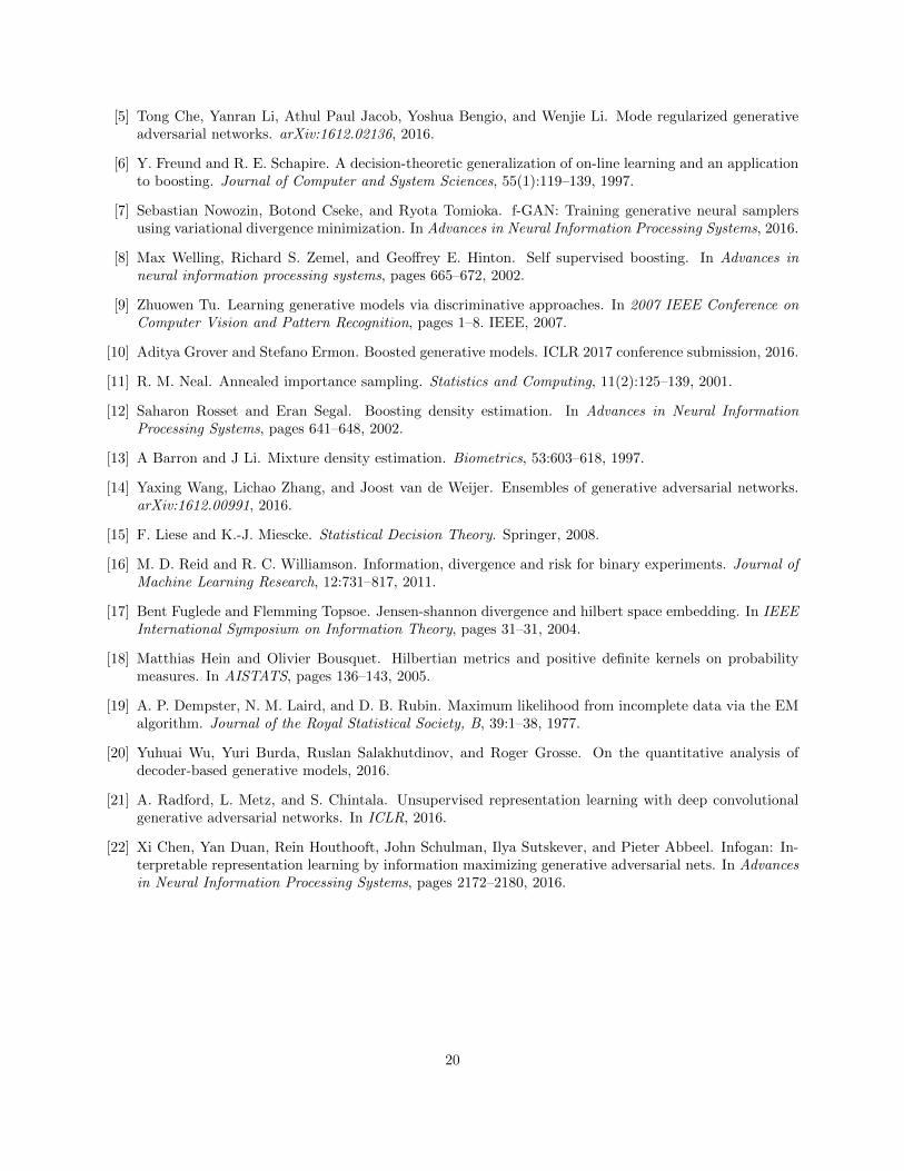
To illustrate the ’meta-algorithm aspect’ of AdaGAN, we also performed experiments with an unrolledGAN [4] instead of a GAN as the base generator. We trained the GANs both with the Jensen-Shannonobjective (2), and with its modified version proposed in [1] (and often considered as the baseline GAN),where log(1−D(G(Z))) is replaced by − log(D(G(Z))). We use the same network architecture as in theother toy experiments. Figure 4 illustrates our results. We find that AdaGAN works with all underlyingGAN algorithms. Note that, where the usual GAN updates the generator and the discriminator once, anunrolled GAN with 5 unrolling steps updates the generator once and the discriminator 1 + 5, i.e. 6 times(and then rolls back 5 steps). Thus, in terms of computation time, training 1 single unrolled GAN roughlycorresponds to doing 3 steps of AdaGAN with a usual GAN. In that sense, Figure 4 shows that AdaGAN(with a usual GAN) significantly outperforms a single unrolled GAN. Additionally, we note that using theJensen-Shannon objective (rather than the modified version) seems to have some mode-regularizing effect.Surprisingly, using unrolling steps makes no significant difference.

Figure 4: Comparison of AdaGAN ran with a GAN (top row) and with an unrolled GAN [4] (bottom).Coverage C of the true data by the model distribution PTmodel, as a function of iterations T . Experimentsare similar to those of Figure 3, but with 10 modes. Top and bottom rows correspond to the usual and theunrolled GAN (with 5 unrolling steps) respectively, trained with the Jensen-Shannon objective (2) on theleft, and with the modified objective originally proposed by [1] on the right. In terms of computation time,one step of AdaGAN with unrolled GAN corresponds to roughly 3 steps of AdaGAN with a usual GAN. Onall images T = 1 corresponds to vanilla unrolled GAN.

B Further details on MNIST/MNIST3 experiments

GAN Architecture We ran AdaGAN on MNIST (28x28 pixel images) using (de)convolutional networkswith batch normalizations and leaky ReLu. The latent space has dimension 100. We used the following

21

architectures:

Generator: 100 x 1 x 1 → fully connected → 7 x 7 x 16 → deconv → 14 x 14 x 8 →→ deconv → 28 x 28 x 4 → deconv → 28 x 28 x 1

Discriminator: 28 x 28 x 1 → conv → 14 x 14 x 16 → conv → 7 x 7 x 32 →→ fully connected → 1

where each arrow consists of a leaky ReLu (with 0.3 leak) followed by a batch normalization, conv and deconvare convolutions and transposed convolutions with 5x5 filters, and fully connected are linear layers with bias.The distribution over Z is uniform over the unit box. We use the Adam optimizer with β1 = 0.5, with 2G steps for 1 D step and learning rates 0.005 for G, 0.001 for D, and 0.0001 for the classifier C that doesthe reweighting of digits. We optimized D and G over 200 epochs and C over 5 epochs, using the originalJensen-Shannon objective (2), without the log trick, with no unrolling and with minibatches of size 128.

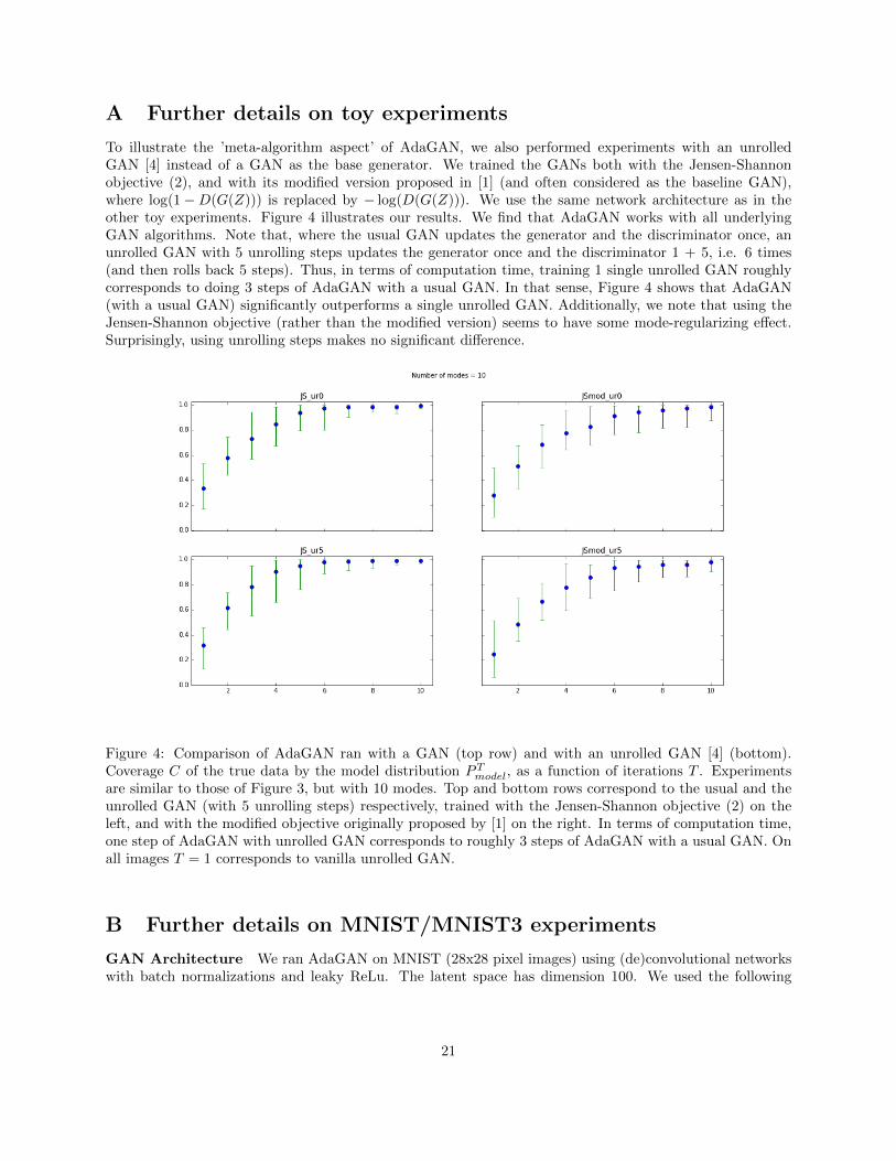
Empirical observations Although we could not find any appropriate metric to measure the increase ofdiversity promoted by AdaGAN, we observed that the re-weighting scheme indeed focuses on digits withvery specific strokes. In Figure 5 for example, we see that after one AdaGAN step, the generator producesoverly thick digits (top left image). Thus AdaGAN puts small weights on the thick digits of the dataset(bottom left) and high weights on the thin ones (bottom right). After the next step, the new GAN producesboth thick and thin digits.

C Proofs

C.1 Proof of Theorem 1

Before proving Theorem 1, we introduce two lemmas. The first one is about the determination of the constantλ, the second one is about comparing the divergences of mixtures.

Lemma 5 Let P and Q be two distributions, γ ∈ [0, 1] and λ ∈ R. The function

g(λ) :=

∫ (λ− γ dQ

dP

)+

dP

is nonnegative, convex, nondecreasing, satisfies g(λ) ≤ λ, and its right derivative is given by

g′+(λ) = P (λ · dP ≥ γ · dQ).

The equationg(λ) = 1− γ

has a solution λ∗ (unique when γ < 1) with λ∗ ∈ [1− γ, 1]. Finally, if P (dQ = 0) ≥ δ for a strictly positiveconstant δ then λ∗ ≤ (1− γ)δ−1.

Proof The convexity of g follows immediately from the convexity of x 7→ (x)+ and the linearity of theintegral. Similarly, since x 7→ (x)+ is non-decreasing, g is non-decreasing.

We define the set I(λ) as follows:

I(λ) := {x ∈ X : λ · dP (x) ≥ γ · dQ(x)}.

Now let us consider g(λ+ ε)− g(λ) for some small ε > 0. This can also be written:

g(λ+ ε)− g(λ) =

∫I(λ)

εdP +

∫I(λ+ε)\I(λ)

(λ+ ε)dP −∫I(λ+ε)\I(λ)

γdQ

= εP (I(λ)) +

∫I(λ+ε)\I(λ)

(λ+ ε)dP −∫I(λ+ε)\I(λ)

γdQ.

22

Figure 5: AdaGAN on MNIST. Bottom row are true MNIST digits with smallest (left) and highest (right)weights after re-weighting at the end of the first AdaGAN step. Those with small weight are thick andresemble those generated by the GAN after the first AdaGAN step (top left). After training with the re-weighted dataset during the second iteration of AdaGAN, the new mixture produces more thin digits (topright).

On the set I(λ+ ε)\I(λ), we have(λ+ ε)dP − γdQ ∈ [0, ε].

So thatεP (I(γ)) ≤ g(λ+ ε)− g(λ) ≤ εP (I(γ)) + εP

(I(λ+ ε)\I(λ)

)= εP (I(λ+ ε))

and thus

limε→0+

g(λ+ ε)− g(λ)

ε= limε→0+

P (I(λ+ ε)) = P (I(λ)).

This gives the expression of the right derivative of g. Moreover, notice that for λ, γ > 0

g′+(λ) = P (λ · dP ≥ γ · dQ) = P

(dQ

dP≤ λ

γ

)= 1− P

(dQ

dP>λ

γ

)≥ 1− γ/λ

by Markov’s inequality.

23

It is obvious that g(0) = 0. By Jensen’s inequality applied to the convex function x 7→ (x)+, we haveg(λ) ≥ (λ− γ)+. So g(1) ≥ 1 − γ. Also, g = 0 on R− and g ≤ λ. This means g is continuous on R andthus reaches the value 1− γ on the interval (0, 1] which shows the existence of λ∗ ∈ (0, 1]. To show that λ∗

is unique we notice that since g(x) = 0 on R−, g is convex and non-decreasing, g cannot be constant on aninterval not containing 0, and thus g(x) = 1− γ has a unique solution for γ < 1.

Also by convexity of g,g(0)− g(λ∗) ≥ −λ∗g′+(λ∗),

which gives λ∗ ≥ (1−γ)/g′+(λ∗) ≥ 1−γ since g′+ ≤ 1. If P (dQ = 0) ≥ δ > 0 then also g′+(0) ≥ δ > 0. Usingthe fact that g′+ is increasing we conclude that λ∗ ≤ (1− γ)δ−1.

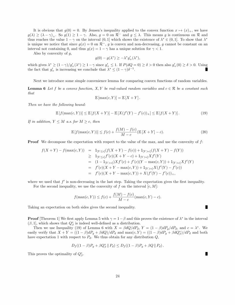
Next we introduce some simple convenience lemma for comparing convex functions of random variables.

Lemma 6 Let f be a convex function, X,Y be real-valued random variables and c ∈ R be a constant suchthat

E [max(c, Y )] = E [X + Y ] .

Then we have the following bound:

E [f(max(c, Y ))] ≤ E [f(X + Y )]− E [X(f ′(Y )− f ′(c))+] ≤ E [f(X + Y )] . (19)

If in addition, Y ≤M a.s. for M ≥ c, then

E [f(max(c, Y ))] ≤ f(c) +f(M)− f(c)

M − c(E [X + Y ]− c). (20)

Proof We decompose the expectation with respect to the value of the max, and use the convexity of f :

f(X + Y )− f(max(c, Y )) = 1[Y≤c](f(X + Y )− f(c)) + 1[Y >c](f(X + Y )− f(Y ))

≥ 1[Y≤c]f′(c)(X + Y − c) + 1[Y >c]Xf

′(Y )

= (1− 1[Y >c])Xf′(c) + f ′(c)(Y −max(c, Y )) + 1[Y >c]Xf

′(Y )

= f ′(c)(X + Y −max(c, Y )) + 1[Y >c]X(f ′(Y )− f ′(c))= f ′(c)(X + Y −max(c, Y )) +X(f ′(Y )− f ′(c))+,

where we used that f ′ is non-decreasing in the last step. Taking the expectation gives the first inequality.For the second inequality, we use the convexity of f on the interval [c,M ]:

f(max(c, Y )) ≤ f(c) +f(M)− f(c)

M − c(max(c, Y )− c).

Taking an expectation on both sides gives the second inequality.

Proof [Theorem 1] We first apply Lemma 5 with γ = 1−β and this proves the existence of λ∗ in the interval(β, 1], which shows that Q∗β is indeed well-defined as a distribution.

Then we use Inequality (19) of Lemma 6 with X = βdQ/dPd, Y = (1 − β)dPg/dPd, and c = λ∗. Weeasily verify that X + Y = ((1 − β)dPg + βdQ)/dPd and max(c, Y ) = ((1 − β)dPg + βdQ∗β)/dPd and bothhave expectation 1 with respect to Pd. We thus obtain for any distribution Q,

Df ((1− β)Pg + βQ∗β ‖Pd) ≤ Df ((1− β)Pg + βQ ‖Pd) .

This proves the optimality of Q∗β .

24

C.2 Proof of Theorem 2

Lemma 7 Let P and Q be two distributions, γ ∈ (0, 1), and λ ≥ 0. The function

h(λ) :=

∫ (1

γ− λdQ

dP

)+

dP

is convex, non-increasing, and its right derivative is given by h′+(λ) = −Q(1/γ ≥ λdQ(X)/dP (X)). Denote∆ := P (dQ(X)/dP (X) = 0). Then the equation

h(λ) =1− γγ

has no solutions if ∆ > 1 − γ, has a single solution λ† ≥ 1 if ∆ < 1 − γ, and has infinitely many or nosolutions when ∆ = 1− γ.

Proof The convexity of h follows immediately from the convexity of x 7→ (a− x)+ and the linearity of theintegral. Similarly, since x 7→ (a− x)+ is non-increasing, h is non-increasing as well.

We define the set J (λ) as follows:

J (λ) :=

{x ∈ X :

1

γ≥ λdQ

dP(x)

}.

Now let us consider h(λ)− h(λ+ ε) for any ε > 0. Note that J (λ+ ε) ⊆ J (λ). We can write:

h(λ)− h(λ+ ε) =

∫J (λ)

(1

γ− λdQ

dP

)dP −

∫J (λ+ε)

(1

γ− (λ+ ε)

dQ

dP

)dP

=

∫J (λ)\J (λ+ε)

(1

γ− λdQ

dP

)dP +

∫J (λ+ε)

(εdQ

dP

)dP

=

∫J (λ)\J (λ+ε)

(1

γ− λdQ

dP

)dP + ε ·Q(J (λ+ ε)).

Note that for x ∈ J (λ) \ J (λ+ ε) we have

0 ≤ 1

γ− λdQ

dP(x) < ε

dQ

dP(x).

This gives the following:

ε ·Q(J (λ+ ε)) ≤ h(λ)− h(λ+ ε) ≤ ε ·Q(J (λ+ ε)) + ε ·Q(J (λ) \ J (λ+ ε)) = ε ·Q(J (λ)),

which shows that h is continuous. Also

limε→0+

h(λ+ ε)− h(λ)

ε= limε→0+

−Q(J (λ+ ε)) = −Q(J (λ)).

It is obvious that h(0) = 1/γ and h ≤ γ−1 for λ ≥ 0. By Jensen’s inequality applied to the convexfunction x 7→ (a− x)+, we have h(λ) ≥

(γ−1 − λ

)+

. So h(1) ≥ γ−1 − 1. We conclude that h may reach the

value (1− γ)/γ = γ−1 − 1 only on [1,+∞). Note that

h(λ)→ 1

γP

(dQ

dP(X) = 0

)=

∆

γ≥ 0 as λ→∞.

Thus if ∆/γ > γ−1−1 the equation h(λ) = γ−1−1 has no solutions, as h is non-increasing. If ∆/γ = γ−1−1then either h(λ) > γ−1 − 1 for all λ ≥ 0 and we have no solutions or there is a finite λ′ ≥ 1 such that

25

h(λ′) = γ−1 − 1, which means that the equation is also satisfied by all λ ≥ λ′, as h is continuous andnon-increasing. Finally, if ∆/γ < γ−1− 1 then there is a unique λ† such that h(λ†) = γ−1− 1, which followsfrom the convexity of h.

Next we introduce some simple convenience lemma for comparing convex functions of random variables.

Lemma 8 Let f be a convex function, X,Y be real-valued random variables such that X ≤ Y a.s., andc ∈ R be a constant such that9

E [min(c, Y )] = E [X] .

Then we have the following lower bound:

E [f(X)− f(min(c, Y ))] ≥ 0.

Proof We decompose the expectation with respect to the value of the min, and use the convexity of f :

f(X)− f(min(c, Y )) = 1[Y≤c](f(X)− f(Y )) + 1[Y >c](f(X)− f(c))

≥ 1[Y≤c]f′(Y )(X − Y ) + 1[Y >c](X − c)f ′(c)

≥ 1[Y≤c]f′(c)(X − Y ) + 1[Y >c](X − c)f ′(c)

= Xf ′(c)−min(Y, c)f ′(c),

where we used the fact that f ′ is non-decreasing in the previous to last step. Taking the expectation we getthe result.

Lemma 9 Let Pg, Pd be two fixed distributions and β ∈ (0, 1). Assume

Pd

(dPgdPd

= 0

)< β.

Let M(Pd, β) be the set of all probability distributions T such that (1 − β)dT ≤ dPd. Then the followingminimization problem:

minT∈M(Pd,β)

Df (T ‖Pg)

has the solution T ∗ with densitydT ∗ := min(dPd/(1− β), λ†dPg),

where λ† is the unique value in [1,∞) such that∫dT ∗ = 1.

Proof We will use Lemma 8 with X = dT (Z)/dPg(Z), Y = dPd(Z)/((1− β)dPg(Z)

), and c = λ∗, Z ∼ Pg.

We need to verify that assumptions of Lemma 8 are satisfied. Obviously, Y ≥ X. We need to show thatthere is a constant c such that ∫

min

(c,

dPd(1− β)dPg

)dPg = 1.

Rewriting this equation we get the following equivalent one:

β =

∫(dPd −min (c(1− β)Pg, dPd)) = (1− β)

∫ (1

1− β− cdPg

dPd

)+

dPd. (21)

Using the fact that

Pd

(dPgdPd

= 0

)< β

9Generally it is not guaranteed that such a constant c always exists. In this result we assume this is the case.

26

we may apply Lemma 7 and conclude that there is a unique c ∈ [1,∞) satisfying (21), which we denote λ†.

To conclude the proof of Theorem 2, observe that from Lemma 9, by making the change of variableT = (Pd − βQ)/(1− β) we can rewrite the minimization problem as follows:

minQ: βdQ≤dPd

Df◦

(Pg ‖

Pd − βQ1− β

)and we verify that the solution has the form dQ†β = 1

β

(dPd − λ†(1− β)dPg

)+

. Since this solution does notdepend on f , the fact that we optimized Df◦ is irrelevant and we get the same solution for Df .

D f-Divergences

Jensen-Shannon This divergence corresponds to

Df (P‖Q) = JS(P,Q) =

∫Xf

(dP

dQ(x)

)dQ(x)

with

f(u) = −(u+ 1) logu+ 1

2+ u log u.

Indeed,

JS(P,Q) :=

∫Xq(x)

−(p(x)

q(x)+ 1

)log

p(x)q(x) + 1

2

+p(x)

q(x)log

p(x)

q(z)

dx

=

∫Xq(x)

(p(x)

q(x)log

2q(x)

p(x) + q(x)+ log

2q(x)

p(x) + q(x)+p(x)

q(z)log

p(x)

q(z)

)dx

=

∫Xp(x) log

2q(x)

p(x) + q(x)+ q(x) log

2q(x)

p(x) + q(x)+ p(x) log

p(x)

q(z)dx

= KL

(Q,

P +Q

2

)+ KL

(P,P +Q

2

).

E Additional experimental results

At each iteration of the boosting approach, different reweighting heuristics are possible. This section containsmore complete results about the following three heuristics:

– Constant β, and using the proposed reweighting scheme given β. See Table 3.

– Reweighting similar to “Cascade GAN” from [14], i.e. keep the top x% of examples, based on thediscriminator corresponding to the previous generator. See Table 4.

– Keep the top x% of examples, based on the discriminator corresponding to the mixture of all previousgenerators. See Table 5.

Note that when properly tuned, each reweighting scheme outperforms the baselines, and have similarperformances when used with few iterations. However, they require an additional parameter to tune, andare worse than the simple β = 1/t heuristic proposed above.

27

Modes : 1 Modes : 2 Modes : 3 Modes : 5 Modes : 7 Modes : 10

Vanilla 0.97 (0.9; 1.0) 0.88 (0.4; 1.0) 0.63 (0.5; 1.0) 0.72 (0.5; 0.8) 0.58 (0.4; 0.8) 0.59 (0.2; 0.7)

Best of T (T=3) 0.99 (1.0; 1.0) 0.96 (0.9; 1.0) 0.91 (0.7; 1.0) 0.80 (0.7; 0.9) 0.84 (0.7; 0.9) 0.70 (0.6; 0.8)

Best of T (T=10) 0.99 (1.0; 1.0) 0.99 (1.0; 1.0) 0.98 (0.8; 1.0) 0.80 (0.8; 0.9) 0.87 (0.8; 0.9) 0.71 (0.7; 0.8)

Ensemble (T=3) 0.99 (1.0; 1.0) 0.98 (0.9; 1.0) 0.93 (0.8; 1.0) 0.78 (0.6; 1.0) 0.85 (0.6; 1.0) 0.80 (0.6; 1.0)

Ensemble (T=10) 1.00 (1.0; 1.0) 0.99 (1.0; 1.0) 1.00 (1.0; 1.0) 0.91 (0.8; 1.0) 0.88 (0.8; 1.0) 0.89 (0.7; 1.0)

Boosted (T=3) 0.99 (1.0; 1.0) 0.99 (0.9; 1.0) 0.98 (0.9; 1.0) 0.91 (0.8; 1.0) 0.91 (0.8; 1.0) 0.86 (0.7; 1.0)

Boosted (T=10) 1.00 (1.0; 1.0) 1.00 (1.0; 1.0) 1.00 (1.0; 1.0) 1.00 (1.0; 1.0) 1.00 (1.0; 1.0) 1.00 (1.0; 1.0)

Modes : 1 Modes : 2 Modes : 3 Modes : 5 Modes : 7 Modes : 10

Vanilla−4.49(−5.4;−4.4)

−6.02(−86.8;−5.3)

−16.03(−59.6;−5.5)

−23.65(−118.8;−5.7)

−126.87(−250.4;−12.8)

−55.51(−185.2;−11.2)

Best of T (T=3)−4.39(−4.6;−4.3)

−5.40(−24.3;−5.2)

−5.57(−23.5;−5.4)

−9.91(−35.8;−5.1)

−36.94(−90.0;−9.7)

−19.12(−59.2;−9.7)

Best of T (T=10)−4.34(−4.4;−4.3)

−5.24(−5.4;−5.2)

−5.45(−5.6;−5.3)

−5.49(−9.4;−5.0)

−9.72(−17.3;−6.5)

−9.12(−16.8;−6.6)

Ensemble (T=3)−4.46(−4.8;−4.4)

−5.59(−6.6;−5.2)

−4.78(−5.5;−4.6)

−14.71(−51.9;−5.4)

−6.70(−28.7;−5.5)

−8.59(−25.4;−6.1)

Ensemble (T=10)−4.52(−4.7;−4.4)

−5.49(−6.6;−5.2)

−4.98(−6.5;−4.6)

−5.44(−6.0;−5.2)

−5.82(−6.4;−5.5)

−6.08(−6.3;−5.7)

Boosted (T=3)−4.50(−4.8;−4.4)

−5.32(−5.8;−5.2)

−4.80(−5.8;−4.6)

−5.39(−19.3;−5.1)

−5.56(−12.4;−5.2)

−8.03(−28.7;−6.1)

Boosted (T=10)−4.55(−4.6;−4.4)

−5.30(−5.5;−5.2)

−5.07(−5.6;−4.7)

−5.25(−5.5;−4.6)

−5.03(−5.5;−4.8)

−5.92(−6.2;−5.6)

Table 2: Performance of the different algorithms on varying number of mixtures of Gaussians. The reportedscores are the median and interval defined by the 5% and 95% percentile (in parenthesis) (see Section4.1.2), over 35 runs for each setting. The top table reports the coverage C, probability mass of Pd coveredby the 5th percentile of Pg defined in Section 4.1.2. The bottom table reports the log likelihood of thetrue data under the model Pg. Note that the 95% interval is not the usual confidence interval measuringthe variance of the experiment itself, but rather measures the stability of the different algorithms (wouldremain even if each experiment was run an infinite number of times). Both the ensemble and the boostingapproaches significantly outperform the vanilla GAN even with just three iterations (i.e. just two additionalcomponents). The boosting approach converges faster to the optimal coverage.

28

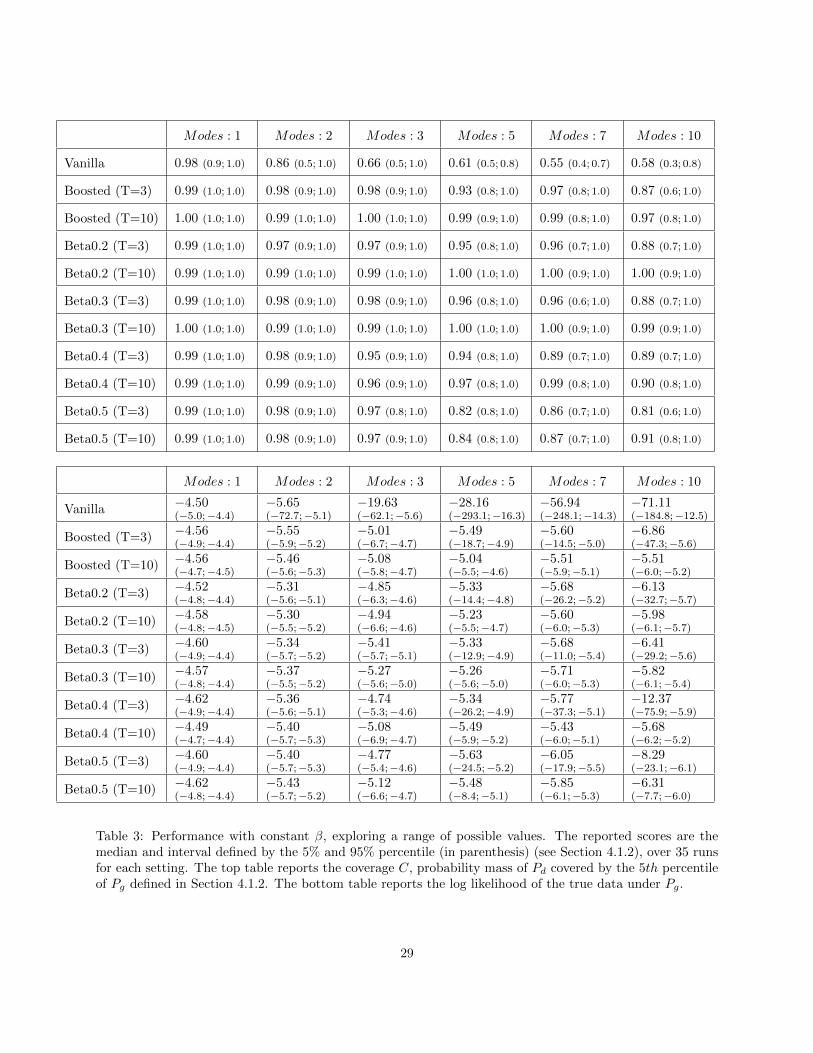
Modes : 1 Modes : 2 Modes : 3 Modes : 5 Modes : 7 Modes : 10

Vanilla 0.98 (0.9; 1.0) 0.86 (0.5; 1.0) 0.66 (0.5; 1.0) 0.61 (0.5; 0.8) 0.55 (0.4; 0.7) 0.58 (0.3; 0.8)

Boosted (T=3) 0.99 (1.0; 1.0) 0.98 (0.9; 1.0) 0.98 (0.9; 1.0) 0.93 (0.8; 1.0) 0.97 (0.8; 1.0) 0.87 (0.6; 1.0)

Boosted (T=10) 1.00 (1.0; 1.0) 0.99 (1.0; 1.0) 1.00 (1.0; 1.0) 0.99 (0.9; 1.0) 0.99 (0.8; 1.0) 0.97 (0.8; 1.0)

Beta0.2 (T=3) 0.99 (1.0; 1.0) 0.97 (0.9; 1.0) 0.97 (0.9; 1.0) 0.95 (0.8; 1.0) 0.96 (0.7; 1.0) 0.88 (0.7; 1.0)

Beta0.2 (T=10) 0.99 (1.0; 1.0) 0.99 (1.0; 1.0) 0.99 (1.0; 1.0) 1.00 (1.0; 1.0) 1.00 (0.9; 1.0) 1.00 (0.9; 1.0)

Beta0.3 (T=3) 0.99 (1.0; 1.0) 0.98 (0.9; 1.0) 0.98 (0.9; 1.0) 0.96 (0.8; 1.0) 0.96 (0.6; 1.0) 0.88 (0.7; 1.0)

Beta0.3 (T=10) 1.00 (1.0; 1.0) 0.99 (1.0; 1.0) 0.99 (1.0; 1.0) 1.00 (1.0; 1.0) 1.00 (0.9; 1.0) 0.99 (0.9; 1.0)

Beta0.4 (T=3) 0.99 (1.0; 1.0) 0.98 (0.9; 1.0) 0.95 (0.9; 1.0) 0.94 (0.8; 1.0) 0.89 (0.7; 1.0) 0.89 (0.7; 1.0)

Beta0.4 (T=10) 0.99 (1.0; 1.0) 0.99 (0.9; 1.0) 0.96 (0.9; 1.0) 0.97 (0.8; 1.0) 0.99 (0.8; 1.0) 0.90 (0.8; 1.0)

Beta0.5 (T=3) 0.99 (1.0; 1.0) 0.98 (0.9; 1.0) 0.97 (0.8; 1.0) 0.82 (0.8; 1.0) 0.86 (0.7; 1.0) 0.81 (0.6; 1.0)

Beta0.5 (T=10) 0.99 (1.0; 1.0) 0.98 (0.9; 1.0) 0.97 (0.9; 1.0) 0.84 (0.8; 1.0) 0.87 (0.7; 1.0) 0.91 (0.8; 1.0)

Modes : 1 Modes : 2 Modes : 3 Modes : 5 Modes : 7 Modes : 10

Vanilla−4.50(−5.0;−4.4)

−5.65(−72.7;−5.1)

−19.63(−62.1;−5.6)

−28.16(−293.1;−16.3)

−56.94(−248.1;−14.3)

−71.11(−184.8;−12.5)

Boosted (T=3)−4.56(−4.9;−4.4)

−5.55(−5.9;−5.2)

−5.01(−6.7;−4.7)

−5.49(−18.7;−4.9)

−5.60(−14.5;−5.0)

−6.86(−47.3;−5.6)

Boosted (T=10)−4.56(−4.7;−4.5)

−5.46(−5.6;−5.3)

−5.08(−5.8;−4.7)

−5.04(−5.5;−4.6)

−5.51(−5.9;−5.1)

−5.51(−6.0;−5.2)

Beta0.2 (T=3)−4.52(−4.8;−4.4)

−5.31(−5.6;−5.1)

−4.85(−6.3;−4.6)

−5.33(−14.4;−4.8)

−5.68(−26.2;−5.2)

−6.13(−32.7;−5.7)

Beta0.2 (T=10)−4.58(−4.8;−4.5)

−5.30(−5.5;−5.2)

−4.94(−6.6;−4.6)

−5.23(−5.5;−4.7)

−5.60(−6.0;−5.3)

−5.98(−6.1;−5.7)

Beta0.3 (T=3)−4.60(−4.9;−4.4)

−5.34(−5.7;−5.2)

−5.41(−5.7;−5.1)

−5.33(−12.9;−4.9)

−5.68(−11.0;−5.4)

−6.41(−29.2;−5.6)

Beta0.3 (T=10)−4.57(−4.8;−4.4)

−5.37(−5.5;−5.2)

−5.27(−5.6;−5.0)

−5.26(−5.6;−5.0)

−5.71(−6.0;−5.3)

−5.82(−6.1;−5.4)

Beta0.4 (T=3)−4.62(−4.9;−4.4)

−5.36(−5.6;−5.1)

−4.74(−5.3;−4.6)

−5.34(−26.2;−4.9)

−5.77(−37.3;−5.1)

−12.37(−75.9;−5.9)

Beta0.4 (T=10)−4.49(−4.7;−4.4)

−5.40(−5.7;−5.3)

−5.08(−6.9;−4.7)

−5.49(−5.9;−5.2)

−5.43(−6.0;−5.1)

−5.68(−6.2;−5.2)

Beta0.5 (T=3)−4.60(−4.9;−4.4)

−5.40(−5.7;−5.3)

−4.77(−5.4;−4.6)

−5.63(−24.5;−5.2)

−6.05(−17.9;−5.5)

−8.29(−23.1;−6.1)

Beta0.5 (T=10)−4.62(−4.8;−4.4)

−5.43(−5.7;−5.2)

−5.12(−6.6;−4.7)

−5.48(−8.4;−5.1)

−5.85(−6.1;−5.3)

−6.31(−7.7;−6.0)

Table 3: Performance with constant β, exploring a range of possible values. The reported scores are themedian and interval defined by the 5% and 95% percentile (in parenthesis) (see Section 4.1.2), over 35 runsfor each setting. The top table reports the coverage C, probability mass of Pd covered by the 5th percentileof Pg defined in Section 4.1.2. The bottom table reports the log likelihood of the true data under Pg.

29

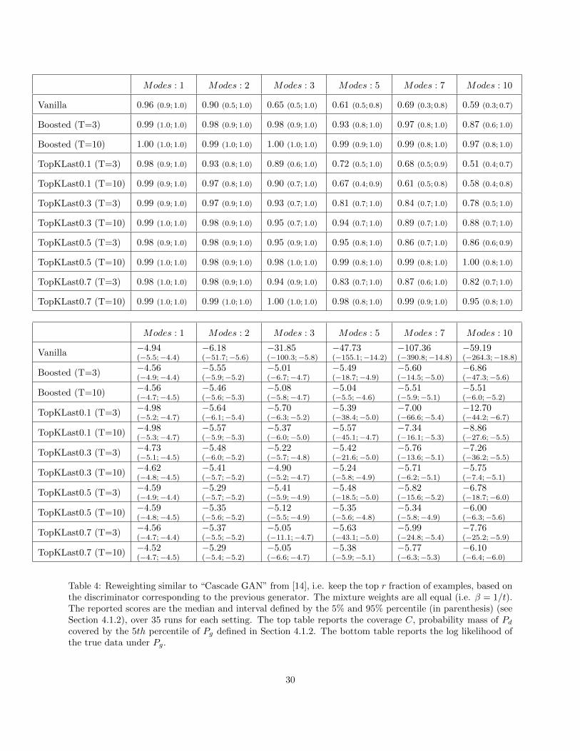
Modes : 1 Modes : 2 Modes : 3 Modes : 5 Modes : 7 Modes : 10

Vanilla 0.96 (0.9; 1.0) 0.90 (0.5; 1.0) 0.65 (0.5; 1.0) 0.61 (0.5; 0.8) 0.69 (0.3; 0.8) 0.59 (0.3; 0.7)

Boosted (T=3) 0.99 (1.0; 1.0) 0.98 (0.9; 1.0) 0.98 (0.9; 1.0) 0.93 (0.8; 1.0) 0.97 (0.8; 1.0) 0.87 (0.6; 1.0)

Boosted (T=10) 1.00 (1.0; 1.0) 0.99 (1.0; 1.0) 1.00 (1.0; 1.0) 0.99 (0.9; 1.0) 0.99 (0.8; 1.0) 0.97 (0.8; 1.0)

TopKLast0.1 (T=3) 0.98 (0.9; 1.0) 0.93 (0.8; 1.0) 0.89 (0.6; 1.0) 0.72 (0.5; 1.0) 0.68 (0.5; 0.9) 0.51 (0.4; 0.7)

TopKLast0.1 (T=10) 0.99 (0.9; 1.0) 0.97 (0.8; 1.0) 0.90 (0.7; 1.0) 0.67 (0.4; 0.9) 0.61 (0.5; 0.8) 0.58 (0.4; 0.8)

TopKLast0.3 (T=3) 0.99 (0.9; 1.0) 0.97 (0.9; 1.0) 0.93 (0.7; 1.0) 0.81 (0.7; 1.0) 0.84 (0.7; 1.0) 0.78 (0.5; 1.0)

TopKLast0.3 (T=10) 0.99 (1.0; 1.0) 0.98 (0.9; 1.0) 0.95 (0.7; 1.0) 0.94 (0.7; 1.0) 0.89 (0.7; 1.0) 0.88 (0.7; 1.0)

TopKLast0.5 (T=3) 0.98 (0.9; 1.0) 0.98 (0.9; 1.0) 0.95 (0.9; 1.0) 0.95 (0.8; 1.0) 0.86 (0.7; 1.0) 0.86 (0.6; 0.9)

TopKLast0.5 (T=10) 0.99 (1.0; 1.0) 0.98 (0.9; 1.0) 0.98 (1.0; 1.0) 0.99 (0.8; 1.0) 0.99 (0.8; 1.0) 1.00 (0.8; 1.0)

TopKLast0.7 (T=3) 0.98 (1.0; 1.0) 0.98 (0.9; 1.0) 0.94 (0.9; 1.0) 0.83 (0.7; 1.0) 0.87 (0.6; 1.0) 0.82 (0.7; 1.0)

TopKLast0.7 (T=10) 0.99 (1.0; 1.0) 0.99 (1.0; 1.0) 1.00 (1.0; 1.0) 0.98 (0.8; 1.0) 0.99 (0.9; 1.0) 0.95 (0.8; 1.0)

Modes : 1 Modes : 2 Modes : 3 Modes : 5 Modes : 7 Modes : 10

Vanilla−4.94(−5.5;−4.4)

−6.18(−51.7;−5.6)

−31.85(−100.3;−5.8)

−47.73(−155.1;−14.2)

−107.36(−390.8;−14.8)

−59.19(−264.3;−18.8)

Boosted (T=3)−4.56(−4.9;−4.4)

−5.55(−5.9;−5.2)

−5.01(−6.7;−4.7)

−5.49(−18.7;−4.9)

−5.60(−14.5;−5.0)

−6.86(−47.3;−5.6)

Boosted (T=10)−4.56(−4.7;−4.5)

−5.46(−5.6;−5.3)

−5.08(−5.8;−4.7)

−5.04(−5.5;−4.6)

−5.51(−5.9;−5.1)

−5.51(−6.0;−5.2)

TopKLast0.1 (T=3)−4.98(−5.2;−4.7)

−5.64(−6.1;−5.4)

−5.70(−6.3;−5.2)

−5.39(−38.4;−5.0)

−7.00(−66.6;−5.4)

−12.70(−44.2;−6.7)

TopKLast0.1 (T=10)−4.98(−5.3;−4.7)

−5.57(−5.9;−5.3)

−5.37(−6.0;−5.0)

−5.57(−45.1;−4.7)

−7.34(−16.1;−5.3)

−8.86(−27.6;−5.5)

TopKLast0.3 (T=3)−4.73(−5.1;−4.5)

−5.48(−6.0;−5.2)

−5.22(−5.7;−4.8)

−5.42(−21.6;−5.0)

−5.76(−13.6;−5.1)

−7.26(−36.2;−5.5)

TopKLast0.3 (T=10)−4.62(−4.8;−4.5)

−5.41(−5.7;−5.2)

−4.90(−5.2;−4.7)

−5.24(−5.8;−4.9)

−5.71(−6.2;−5.1)

−5.75(−7.4;−5.1)

TopKLast0.5 (T=3)−4.59(−4.9;−4.4)

−5.29(−5.7;−5.2)

−5.41(−5.9;−4.9)

−5.48(−18.5;−5.0)

−5.82(−15.6;−5.2)

−6.78(−18.7;−6.0)

TopKLast0.5 (T=10)−4.59(−4.8;−4.5)

−5.35(−5.6;−5.2)

−5.12(−5.5;−4.9)

−5.35(−5.6;−4.8)

−5.34(−5.8;−4.9)

−6.00(−6.3;−5.6)

TopKLast0.7 (T=3)−4.56(−4.7;−4.4)

−5.37(−5.5;−5.2)

−5.05(−11.1;−4.7)

−5.63(−43.1;−5.0)

−5.99(−24.8;−5.4)

−7.76(−25.2;−5.9)

TopKLast0.7 (T=10)−4.52(−4.7;−4.5)

−5.29(−5.4;−5.2)

−5.05(−6.6;−4.7)

−5.38(−5.9;−5.1)

−5.77(−6.3;−5.3)

−6.10(−6.4;−6.0)

Table 4: Reweighting similar to “Cascade GAN” from [14], i.e. keep the top r fraction of examples, based onthe discriminator corresponding to the previous generator. The mixture weights are all equal (i.e. β = 1/t).The reported scores are the median and interval defined by the 5% and 95% percentile (in parenthesis) (seeSection 4.1.2), over 35 runs for each setting. The top table reports the coverage C, probability mass of Pdcovered by the 5th percentile of Pg defined in Section 4.1.2. The bottom table reports the log likelihood ofthe true data under Pg.

30

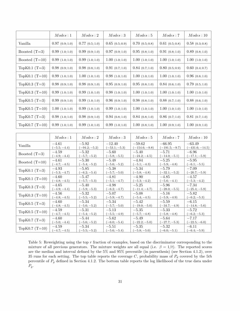
Modes : 1 Modes : 2 Modes : 3 Modes : 5 Modes : 7 Modes : 10

Vanilla 0.97 (0.9; 1.0) 0.77 (0.5; 1.0) 0.65 (0.5; 0.9) 0.70 (0.5; 0.8) 0.61 (0.5; 0.8) 0.58 (0.3; 0.8)

Boosted (T=3) 0.99 (1.0; 1.0) 0.99 (0.9; 1.0) 0.97 (0.9; 1.0) 0.95 (0.8; 1.0) 0.91 (0.8; 1.0) 0.89 (0.8; 1.0)

Boosted (T=10) 0.99 (1.0; 1.0) 0.99 (1.0; 1.0) 1.00 (1.0; 1.0) 1.00 (1.0; 1.0) 1.00 (1.0; 1.0) 1.00 (1.0; 1.0)

TopK0.1 (T=3) 0.98 (0.9; 1.0) 0.98 (0.8; 1.0) 0.91 (0.7; 1.0) 0.84 (0.7; 1.0) 0.80 (0.5; 0.9) 0.60 (0.4; 0.7)

TopK0.1 (T=10) 0.99 (1.0; 1.0) 1.00 (1.0; 1.0) 0.98 (1.0; 1.0) 1.00 (1.0; 1.0) 1.00 (1.0; 1.0) 0.96 (0.8; 1.0)

TopK0.3 (T=3) 0.98 (0.9; 1.0) 0.98 (0.9; 1.0) 0.95 (0.9; 1.0) 0.95 (0.8; 1.0) 0.84 (0.6; 1.0) 0.79 (0.5; 1.0)

TopK0.3 (T=10) 0.99 (1.0; 1.0) 0.99 (1.0; 1.0) 0.98 (1.0; 1.0) 1.00 (1.0; 1.0) 1.00 (1.0; 1.0) 1.00 (1.0; 1.0)

TopK0.5 (T=3) 0.99 (0.9; 1.0) 0.99 (1.0; 1.0) 0.96 (0.9; 1.0) 0.98 (0.8; 1.0) 0.88 (0.7; 1.0) 0.88 (0.6; 1.0)

TopK0.5 (T=10) 1.00 (1.0; 1.0) 0.99 (1.0; 1.0) 0.99 (1.0; 1.0) 1.00 (1.0; 1.0) 1.00 (1.0; 1.0) 1.00 (1.0; 1.0)

TopK0.7 (T=3) 0.98 (1.0; 1.0) 0.98 (0.9; 1.0) 0.94 (0.8; 1.0) 0.84 (0.8; 1.0) 0.86 (0.7; 1.0) 0.81 (0.7; 1.0)

TopK0.7 (T=10) 0.99 (1.0; 1.0) 0.99 (1.0; 1.0) 0.99 (1.0; 1.0) 1.00 (0.8; 1.0) 1.00 (0.9; 1.0) 1.00 (0.9; 1.0)

Modes : 1 Modes : 2 Modes : 3 Modes : 5 Modes : 7 Modes : 10

Vanilla−4.61(−5.5;−4.4)

−5.92(−94.2;−5.2)

−12.40(−53.1;−5.3)

−59.62(−154.6;−9.8)

−66.95(−191.5;−9.7)

−63.49(−431.6;−14.5)

Boosted (T=3)−4.59(−4.9;−4.4)

−5.32(−5.7;−5.2)

−5.60(−5.8;−5.5)

−5.40(−24.2;−4.5)

−5.71(−14.0;−5.1)

−6.96(−17.1;−5.9)

Boosted (T=10)−4.61(−4.7;−4.5)

−5.30(−5.4;−5.2)

−5.48(−5.6;−5.2)

−4.84(−5.1;−4.3)

−5.25(−5.9;−4.8)

−5.95(−6.1;−5.5)

TopK0.1 (T=3)−4.93(−5.3;−4.7)

−5.85(−6.2;−5.4)

−5.38(−5.7;−5.0)

−5.34(−5.8;−4.8)

−5.79(−32.1;−5.2)

−7.09(−20.7;−5.9)

TopK0.1 (T=10)−4.60(−4.8;−4.5)

−5.47(−5.7;−5.3)

−4.81(−5.1;−4.7)

−4.90(−5.3;−4.2)

−4.85(−5.6;−4.1)

−4.57(−5.3;−4.2)

TopK0.3 (T=3)−4.65(−4.9;−4.4)

−5.40(−5.9;−5.3)

−4.98(−6.2;−4.7)

−5.25(−11.4;−4.7)

−5.96(−28.0;−5.5)

−7.34(−25.4;−5.9)

TopK0.3 (T=10)−4.56(−4.8;−4.5)

−5.32(−5.5;−5.2)

−5.07(−5.9;−4.7)

−5.08(−5.4;−4.5)

−5.16(−5.9;−4.9)

−5.82(−6.2;−5.3)

TopK0.5 (T=3)−4.60(−4.8;−4.5)

−5.34(−5.6;−5.2)

−5.34(−5.7;−5.0)

−5.42(−19.0;−5.0)

−5.59(−34.7;−4.9)

−6.15(−14.8;−5.6)

TopK0.5 (T=10)−4.59(−4.7;−4.5)

−5.31(−5.4;−5.2)

−5.13(−5.5;−4.9)

−5.35(−5.7;−4.8)

−5.33(−5.8;−4.8)

−5.72(−6.2;−5.3)

TopK0.7 (T=3)−4.60(−5.0;−4.4)

−5.44(−5.6;−5.2)

−5.62(−6.0;−5.4)

−5.49(−22.2;−5.0)

−5.64(−27.7;−5.3)

−7.17(−22.5;−6.0)

TopK0.7 (T=10)−4.59(−4.7;−4.5)

−5.34(−5.5;−5.2)

−5.51(−5.6;−5.4)

−5.35(−5.8;−5.0)

−5.32(−6.0;−5.1)

−6.11(−6.4;−5.9)

Table 5: Reweighting using the top r fraction of examples, based on the discriminator corresponding to themixture of all previous generators. The mixture weights are all equal (i.e. β = 1/t). The reported scoresare the median and interval defined by the 5% and 95% percentile (in parenthesis) (see Section 4.1.2), over35 runs for each setting. The top table reports the coverage C, probability mass of Pd covered by the 5thpercentile of Pg defined in Section 4.1.2. The bottom table reports the log likelihood of the true data underPg.

31