Embed Size (px)
DESCRIPTION
ada
Citation preview

ERD
C/G
SL T
R-08
-24
Modular Protective Systems for Future Force Assets
Flexural and Tensile Properties of Thin, Very High-Strength, Fiber-Reinforced Concrete Panels
Michael J. Roth September 2008
Geo
tech
nica
l and
Str
uctu
res
Labo
rato
ry
Approved for public release; distribution is unlimited.

Modular Protective Systems for Future Force Assets
ERDC/GSL TR-08-24 September 2008
Flexural and Tensile Properties of Thin, Very High-Strength, Fiber-Reinforced Concrete Panels
Michael J. Roth Geotechnical and Structures Laboratory U.S. Army Engineer Research and Development Center 3909 Halls Ferry Road Vicksburg, MS 39180-6199
Final report Approved for public release; distribution is unlimited.
Prepared for Headquarters, U.S. Army Corps of Engineers Washington, DC 20314-1000
Under Work Unit A1450, Advanced Concrete Based Armor Materials

ERDC/GSL TR-08-24 ii
Abstract: This research was conducted to characterize the flexural and tensile characteristics of thin, very high-strength, discontinuously reinforced concrete panels jointly developed by the U.S. Army Engineer Research and Development Center and U.S. Gypsum Corporation. Panels were produced from a unique blend of cementitous material and fiberglass reinforcing fibers, achieving compressive strength and fracture toughness levels that far exceeded those of typical concrete.
The research program included third-point flexural experiments, novel direct tension experiments, implementation of micromechanically based analytical models, and development of finite element numerical models. The experimental, analytical, and numerical efforts were used conjunctively to determine parameters such as elastic modulus, first-crack strength, post-crack modulus, and fiber/matrix interfacial bond strength. Furthermore, analytical and numerical models imple-mented in the work showed potential for use as design tools in future engineered material improvements.
DISCLAIMER: The contents of this report are not to be used for advertising, publication, or promotional purposes. Citation of trade names does not constitute an official endorsement or approval of the use of such commercial products. All product names and trademarks cited are the property of their respective owners. The findings of this report are not to be construed as an official Department of the Army position unless so designated by other authorized documents. DESTROY THIS REPORT WHEN NO LONGER NEEDED. DO NOT RETURN IT TO THE ORIGINATOR.

iii
TABLE OF CONTENTS
Page
ABSTRACT............................................................................................................... ii
LIST OF TABLES..................................................................................................... v
LIST OF FIGURES ................................................................................................... vi
PREFACE.................................................................................................................. xi
CHAPTER
I. INTRODUCTION......................................................................................... 1
1.1 Background.................................................................................. 1 1.2 Material study, multiscale perspective......................................... 3 1.3 VHSC material development ....................................................... 4 1.4 Research objective ....................................................................... 5 1.5 Research approach ....................................................................... 6 II. FLEXURAL EXPERIMENTS ..................................................................... 8
2.1 Testing procedure and equipment................................................ 8 2.2 Panel test specimens .................................................................... 12 2.3 Experimental results..................................................................... 14 III. DIRECT TENSION EXPERIMENTS .......................................................... 33
3.1 Testing procedure and equipment................................................ 34 3.2 Tension test specimens ................................................................ 39 3.3 Experimental results..................................................................... 40 3.4 Elastic strain state analysis........................................................... 49 3.5 Elastic stress state analysis and tensile modulus calculation ....... 61 3.6 FE mesh refinement analysis ....................................................... 73 3.7 Post-crack tensile softening ......................................................... 76 IV. MICROMECHANICAL MODELS .............................................................. 87
4.1 Single fiber pullout model ........................................................... 88 4.2 Single fiber pullout model, inclination angle effects ................... 98 4.3 Composite material response model, pullout failure only ........... 102 4.4 Composite material response model, fiber rupture effects .......... 110 4.5 Composite material response model, slip softening effects......... 122 4.6 Summary of micromechanical model results............................... 127

iv
V. FLEXURAL FINITE ELEMENT MODEL ................................................... 132
5.1 Shell element model with elastic-plastic material model ............ 133 5.2 Shell element model with concrete damage material model ....... 144 VI. SUMMARY AND CONCLUSIONS........................................................... 159
6.1 Summary ...................................................................................... 159 6.2 Results and conclusions ............................................................... 160 6.3 Recommended panel and material properties .............................. 167 6.4 Recommendations for future research ......................................... 170 BIBLIOGRAPHY...................................................................................................... 172 REPORT DOCUMENTATION PAGE

v
LIST OF TABLES
TABLE Page
2.1 Mechanical properties of NEG AR2500 H-103 fiberglass..................... 13
2.2 Flexural test specimens, water absorption .............................................. 15
2.3 Flexural test specimens, mechanical properties...................................... 27
3.1 Direct tension Test 1, elastic strain analysis........................................... 54
3.2 Direct tension Test 2, elastic strain analysis........................................... 55
3.3 Direct tension Test 4, elastic strain analysis........................................... 56
3.4 Direct tension Test 1, elastic stress analysis and tensile modulus calculation........................................................................... 69
3.5 Direct tension Test 2, elastic stress analysis and tensile
modulus calculation .......................................................................... 70
3.6 Direct tension Test 4, elastic stress analysis and tensile modulus calculation .......................................................................... 71
3.7 Tensile modulus comparison, tension tests and flexural tests ................ 73
4.1 Published fiber/matrix bond strengths for various fiber types................ 93
4.2 Published snubbing coefficients for various fiber types......................... 99
6.1 Recommended panel and material properties......................................... 168

vi
LIST OF FIGURES
FIGURE Page
1.1 Length scale frameworks of a multiscale material study........................ 4
2.1 Flexural test support fixture.................................................................... 10
2.2 Flexural test loading head (with spring modifications) .......................... 10
2.3 Test specimen loaded at third-points ...................................................... 11
2.4 Flexural test specimen being cut on water-jet machine.......................... 14
2.5 Test 1 flexural test: Load vs. third-point displacement history .............. 17
2.6 Test 2 flexural test: Load vs. third-point displacement history .............. 17
2.7 Test 3 flexural test: Load vs. third-point displacement history .............. 18
2.8 Test 4 flexural test: Load vs. third-point displacement history .............. 18
2.9 Test 5 flexural test: Load vs. third-point displacement history .............. 19
2.10 Test 6 flexural test: Load vs. third-point displacement history .............. 19
2.11 Test 7 flexural test: Load vs. third-point displacement history .............. 20
2.12 Test 8 flexural test: Load vs. third-point displacement history .............. 20
2.13 Test 9 flexural test: Load vs. third-point displacement history .............. 21
2.14 Test 10 flexural test: Load vs. third-point displacement history ............ 21
2.15 Flexural tests: Load-displacement history comparisons......................... 28
2.16 Test 7, multiple crack initiation .............................................................. 30
2.17 Test 7, final single crack failure ............................................................. 30
2.18 Flexural test: Response envelope and mean response function.............. 32
3.1 Direct tension test, non-uniform crack opening ..................................... 36

vii
3.2 Direct tension specimen with rigid connection to fixture....................... 37
3.3 Direct tension specimen, dimensions and strain gage layout ................. 38
3.4 Direct tension specimen with epoxied steel end caps............................. 40
3.5 Tension Test 1, cracked specimen at test completion............................. 41
3.6 Tension test strain gage designations, “A” side...................................... 42
3.7 Tension Test 1: Load-strain history, gage A1 vs. gage B1..................... 43
3.8 Tension Test 1: Load-strain history, gage A2 vs. gage B2..................... 44
3.9 Tension Test 1: Load-strain history, gage A3 vs. gage B3..................... 44
3.10 Tension Test 2: Load-strain history, gage A1 vs. gage B1..................... 45
3.11 Tension Test 2: Load-strain history, gage A2 vs. gage B2..................... 45
3.12 Tension Test 2: Load-strain history, gage A3 vs. gage B3..................... 46
3.13 Tension Test 4: Load-strain history, gage A1 vs. gage B1..................... 46
3.14 Tension Test 4: Load-strain history, gage A2 vs. gage B2..................... 47
3.15 Tension test end cap, threaded connector welded to bar stock............... 48
3.16 Tension specimen free body diagram..................................................... 51
3.17 Tension specimen, strain resolution with tension and compression strain state .......................................................................................... 51
3.18 Tension specimen, strain resolution with tension only strain state ........ 51
3.19 Tension test 1, elastic strain correction, gages A1 and B1 ..................... 56
3.20 Tension test 1, elastic strain correction, gages A2 and B2 ..................... 57
3.21 Tension test 1, elastic strain correction, gages A3 and B3 ..................... 57
3.22 Tension test 2, elastic strain correction, gages A1 and B1 ..................... 58
3.23 Tension test 2, elastic strain correction, gages A2 and B2 ..................... 58
viii
3.24 Tension test 2, elastic strain correction, gages A3 and B3 ..................... 59
3.25 Tension test 4, elastic strain correction, gages A1 and B1 ..................... 59
3.26 Tension test 4, elastic strain correction, gages A2 and B2 ..................... 60
3.27 Tension test FE model ............................................................................ 63
3.28 Tension test: FE load application ........................................................... 64
3.29 Tension test: FE axial stress contours at 1,100 lb (4,893 N) load .......... 66
3.30 Tension test: Gage A1 FE and nominal stress-load histories ............ 67
3.31 Tension test: Gage A2 FE and nominal stress-load histories ................. 68
3.32 Mesh refinement analysis, A1 location .................................................. 74
3.33 Mesh refinement analysis, A1 location (smaller scale) .......................... 74
3.34 Mesh refinement analysis, A2 location .................................................. 75
3.35 Mesh refinement analysis, A2 location (smaller scale) .......................... 75
3.36 Tension Tests 1 and 2: Stress-crack opening relationship...................... 77
3.37 FE stress distribution and concentration at tension test specimen notch .................................................................................. 81
3.38 Recommended stress versus crack opening relationship for VHSC ...... 82
3.39 Tension test specimen, broken glass fibers............................................. 84
3.40 Tension test specimen, bridging fibers at test completion...................... 85
3.41 Tension test specimen, mass of fibers—some broken and some aligned with crack .................................................................... 85
3.42 Tension test specimen, fibers pulled from cementitous matrix .............. 86
4.1 Single fiber pullout model at various load stages................................... 90
4.2 Single fiber axial load versus crack opening, debonding phase ............. 96

ix
4.3 Single fiber axial load versus crack opening, debond to pullout transition................................................................................ 97
4.4 Single fiber axial load versus crack opening, complete pullout response ................................................................................. 97
4.5 Single fiber axial load versus crack opening during debonding (fiber at angle to crack), τifmax = 150 psi (1 MPa) .............................. 101
4.6 Single fiber axial load versus crack opening during debonding (fiber at angle to crack), τifmax = 600 psi (4.1 MPa) ........................... 101
4.7 Composite bridging stress as a function of crack opening, debonding phase ................................................................................ 106
4.8 Composite bridging stress as a function of crack opening, debonding and pullout phases............................................................ 107
4.9 Composite bridging stress as a function of crack opening, corrected for pre-crack linear-elastic response of the matrix ............................ 109
4.10 Fiber rupture failure envelope, τifmax = 600 psi (4.1 MPa)...................... 113
4.11 Fiber rupture failure envelope, τifmax = 2,100 (14.5 MPa) and 5,000 psi (34.5 MPa)................................................................... 115
4.12 Composite bridging stress functions from rupture and pullout model (uncorrected for pre-crack stress state) .............................................. 119 4.13 Composite bridging stress functions from rupture and pullout model (corrected for pre-crack stress state) .................................................. 121 4.14 Linear and exponential fiber bond strength decay functions.................. 125
4.15 Composite bridging stress functions with linear and exponential bond strength decay (pullout model) ................................................. 126
4.16 Composite bridging stress functions with linear and exponential bond strength decay (rupture and pullout model).............................. 126
4.17 Recommended bridging function from direct tension experiments ....... 129
x
5.1 Discretized shell element model with applied loads and boundary conditions........................................................................... 134
5.2 Elastic-plastic stress versus strain curve................................................. 135
5.3 FE shell model results versus mean experimental curve (elastic-plastic material model).......................................................... 137
5.4 3 IP stress versus load curve, center element ......................................... 139
5.5 7 IP stress versus load curve, center element ......................................... 139
5.6 Integration point and S11 stress distribution for 3 IP and 7 IP linear shell elements .......................................................................... 141
5.7 FE load-deflection curves, adjusted yield stress for 5, 7, and 19 IP models ...................................................................................... 144
5.8 Initial tensile failure curve definition for concrete damage model......... 147
5.9 Concrete damage model results for 3, 7, 9 and 15 integration points .... 148
5.10 Concrete damage model, center element stress state for 3 IP model...... 149
5.11 Truncated tensile failure curve definition for concrete damage model.................................................................................... 152
5.12 Concrete damage model results with truncated tensile failure function................................................................................... 153
5.13 Center element S11 stress states, concrete damage model with truncated tensile failure function ....................................................... 154
5.14 Revised tensile failure functions from iterative calculations.................. 156
5.15 Third-point displacement comparison, computed versus experimental (concrete damage material model).................................................... 156
6.1 Recommended load-displacement resistance function (third-point loading, 10-in. wide panel, 36-in. span) ............................................ 169
6.2 Recommended tensile failure function (crack bridging stress function) 169

xi
PREFACE
The research described herein was conducted as part of the research program
ATO IV.EN.2005.04, “Modular Protective Systems for Future Force Assets,” sponsored
by Headquarters, U.S. Army Corps of Engineers. Research was conducted as a part of
Work Unit A1450, “Advanced Concrete Based Armor Materials.” Work unit manager
was Toney Cummins, Survivability Engineering Branch (SvEB), Geosciences and
Structures Division (GSD), Geotechnical and Structures Laboratory (GSL), U.S. Army
Engineer Research and Development Center (ERDC).
This report was prepared by Michael J. Roth, SvEB, in partial fulfillment of the
requirements for the degree of Master of Science in Civil Engineering, Mississippi State
University (MSU). Thesis committee members were Dr. Christopher Eamon, MSU;
Dr. Thomas Slawson, SvEB; and Dr. Stanley C. Woodson, Research Group, GSD.
Additional support was provided by Joe Tom and Dan Wilson, Concrete and Materials
Branch, Engineering Systems and Materials Division, GSL, and Alex Jackson, SvEB, in
the design and execution of the flexural and direct tension experimental programs.
Assistance from Omar Flores, summer student, University of Puerto Rico, Mayaguez,
was provided in development of finite element models for the direct tension test analysis.
Work was conducted under the general supervision of Pamela G. Kinnebrew,
Chief, SvEB; Dr. Robert L. Hall, Chief, GSD; Dr. William P. Grogan, Deputy Director,
GSL; and Dr. David W. Pittman, Director, GSL.
COL Gary E. Johnston was Commander and Executive Director of ERDC.
Dr. James R. Houston was Director.

1
CHAPTER I
INTRODUCTION 1.1 Background
As part of the continued development of new and innovative construction
materials for applications in civil, structural, and military engineering, high performance
concrete has maintained itself as an area of directed focus. Advancements in the science
and technology of cementitous materials have brought about mesoscale to sub-microscale
material engineering (through development of concepts such as particle packing theory,
macro-defect free concrete, heat and pressure treatment to facilitate molecular structure
manipulation, and microfiber inclusion to inhibit growth and localization of microcracks),
and have resulted in materials with unconfined compressive strengths as high as
29,000 psi (200 MPa) or greater [1-4]. High-strength and ultra-high-strength concrete,
with unconfined compressive strengths of 10,000 psi (69 MPa) to 25,000 psi (172 MPa)
and greater, have experienced continued growth in commercial application as the
community’s state of knowledge and production capability have advanced [5-8].
In conjunction with enhancement of unconfined compressive strength, significant
research has been conducted to develop means of improving the tensile characteristics of
cementitous materials. The classical approach of incorporating discrete reinforcing steel
has been augmented with the capability to reinforce with other, more advanced, materials
such as ultra-high tensile strength steel meshes (460 ksi (3.2 GPa) or greater),

2
fiber-reinforced plastics, carbon-fiber strands, glass-fiber strands, and other high-strength
and/or high-ductility fibers such as continuous aramid or polypropylene strands [9-13]. A
significant portion of this research on advanced reinforcement has focused on continuous
strand applications, analogous to the way that typical deformed bars are incorporated into
concrete members. However, research has also been conducted on the inclusion and
effect of discontinuous reinforcement.
Discontinuous reinforcement, consisting of short, randomly distributed fibers, has
been studied experimentally, analytically, and micromechanically with regard to its
influence on concrete’s tensile characteristics [14-20]. Considering that individual fiber
lengths may be as small as 0.5 in. (12.7 mm) and fiber diameters as small as 0.02 in.
(0.5 mm) or smaller, from a macroscopic viewpoint, it is reasonable to consider the fibers
as a basic constitutive component of the concrete, in contrast to the typical discrete
treatment of deformed bars or continuous strand reinforcement. With refinement in scale,
the fibers have been studied explicitly with respect to their interaction with the
cementitous matrix [21-38]; however, the simple stochastic nature of their dispersion,
concentration, and orientation has necessitated a macroscale homogenization of their
influence on a concrete member’s global response to load. Only in more recent research
have numerical models been developed to consider discontinuous fiber influence at the
sub-macroscopic level [39-45], but they have certainly not been made applicable to
widespread community use.
Because of the stochastic nature of random, discontinuous fiber reinforcing, and
the subsequent challenges associated with explicitly defining its influence on global

3
member response, standards have not been developed for its use as a primary reinforcing
mechanism in architectural or structural components. Rather, its use in design has been
limited to enhancement of secondary effects such as crack-width control and bond
strength between concrete and reinforcement. However, as shown in this research effort
and many others, the discontinuous fibers can have a significant influence on post-crack
ductility of an otherwise unreinforced concrete member, and therefore could be of
tangible benefit in the design of certain concrete components if sufficient knowledge can
be obtained to safely develop guidance for its use.
1.2 Material study, multiscale perspective
Within this report, terms such as macroscale, mesoscale, and microscale are used
when considering various aspects of the studied material. These stem from viewing the
heterogeneous material in a “multiscale” framework, implying that based on the frame of
reference, certain material constituents—and their interaction—may be studied discretely,
while smaller components are considered in a homogenized representation of everything
finer than the smallest scale considered. The benefit of studying materials in this manner
arises from the capability to derive global characteristics from basic interaction between
constitutive components—allowing for significant increases in material design and
analysis capabilities through better understanding of the fundamental mechanics
governing global response.
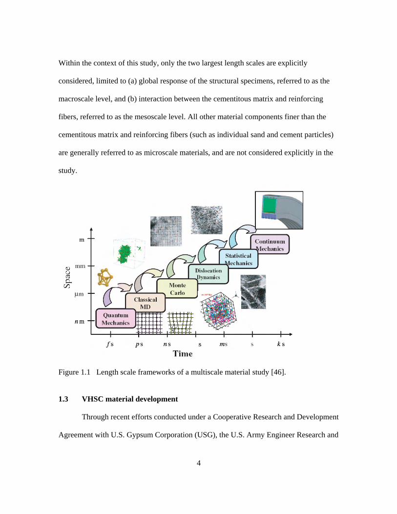
As shown in Figure 1, length scales considered within a multiscale framework can
be extensive, ranging from global response of a structural member (length scale of 1 m)
to molecular dynamics and atomistic models (length scale of 1×10⁻⁶ m to 1×10⁻⁹ m).
4
Within the context of this study, only the two largest length scales are explicitly
considered, limited to (a) global response of the structural specimens, referred to as the
macroscale level, and (b) interaction between the cementitous matrix and reinforcing
fibers, referred to as the mesoscale level. All other material components finer than the
cementitous matrix and reinforcing fibers (such as individual sand and cement particles)
are generally referred to as microscale materials, and are not considered explicitly in the
study.
Figure 1.1 Length scale frameworks of a multiscale material study [46].
1.3 VHSC material development
Through recent efforts conducted under a Cooperative Research and Development
Agreement with U.S. Gypsum Corporation (USG), the U.S. Army Engineer Research and

5
Development Center (ERDC) has developed a new very high-strength, discontinuous
fiber-reinforced concrete material (VHSC) with potential applications, in
mass-producible thin panel form, to both military and civilian use. Utilized in the con-
crete production is a unique blend of aggregate, cementitous, and pozollanic materials,
which span a range of length scales between 0.05 microns and 0.02 in. (0.5 mm). With
proper gradation of the material at each scale, complimentary properties for each material
(such as coefficient of thermal expansion), and an effective water-reducing admixture to
facilitate a very low water-to-cement ratio (w/c ≈ 0.2), an unconfined compressive
strength of approximately 21,500 psi (148 MPa) is achieved. Due to weight and size
requirements dictated by application constraints, the cast VHSC panels are limited to a
nominal 0.5 in. (12.7 mm) thickness, which prevents usage of conventional reinforcement
to provide tensile capacity. Wire meshes (such as those used in ferrocement) have not
been used based on production and cost constraints and, therefore, randomly distributed
fiberglass reinforcing has been used as the only means of tensile reinforcement in the thin
VHSC panels.
1.4 Research objective
To incorporate ERDC’s newly developed VHSC panels into the desired applica-
tions, an understanding of their response to load was required so that panel configurations
and the necessary support structures could be properly designed. Furthermore, to intelli-
gently design future improvements in panel performance (in terms of hardened charac-
teristics such as strength or ductility) an understanding of the constitutive components’
contribution to desirable or undesirable performance attributes was also needed.

6
However, because thin ultra-high strength, discontinuously reinforced concrete structural
components represent a new type of construction material—in contrast to classical, con-
ventionally reinforced concrete members—standards for design and analysis of the pan-
els’ performance were not available for use.
The above considered, the objective of this research was to use experimental,
analytical, and numerical means to characterize the response of the 0.5-in.-thick
(12.7-mm) panels to flexural and tensile loads. Additionally, micromechanically based,
analytical approaches published in the literature were used to study the new ERDC
material at the mesoscale level in order to better understand the interaction between fibers
and the cementitous matrix—providing knowledge necessary to design future global
performance improvements through modifications at the material level.
1.5 Research approach
To accomplish the previously stated research objectives, a multi-faceted approach
was developed that utilized experimental, analytical, and numerical methods to study the
VHSC material and hardened panels. Components of the research program included:
• Ten closed-loop, third-point bending experiments to characterize the panels’
pre- and post-crack response in flexure.
• Limited set of closed-loop, direct tension experiments used to support findings
from the flexural experiments and directly measure the VHSC material’s post-
crack ductility.
• Implementation of micromechanically based, analytical models to estimate the
material’s macroscopic tensile response based on mesoscale consideration of the

7
interaction between fibers and cementitous matrix. Model results were compared
to the direct tension experiments to improve understanding of the mechanics
governing tensile failure in the material and support the design of future material
improvements.
• Development of numerical models based on the third-point bending experiments.
Multiple materials models were implemented, including a simple elastic-plastic
model and a more complex concrete damage model. Experimentally determined
panel characteristics, such as initial linear-elastic modulus, were used in the
elastic-plastic model, and a tensile failure function (determined from the direct
tension experiments and micromechanical models) was used in the concrete
damage model.

8
CHAPTER II
FLEXURAL EXPERIMENTS
In the applications of current interest, the most common loading condition
expected for the thin VHSC panels was simply supported bending. Therefore, it was
desired to experimentally determine the flexural resistance of a sufficient number of
panels so that basic characteristics of their pre- and post-crack response in flexure could
be determined. In turn, data collected from the experiments were expected to support
engineering level design tools and higher fidelity numerical model development for
specific applications desired by ERDC.
2.1 Testing procedure and equipment
Response in flexure of the 0.5-in.-thick (12.7-mm) VHSC panels was
experimentally determined by means of 10 third-point loading tests. The tests were
conducted in accordance with ASTM C947-03 [47] on an MTS testing machine, with a
110-kip (489-kN) load cell and a linear variable displacement transducer (LVDT)
monitored loading head. The loading system and LVDT were connected in a closed-loop
manner, which provided displacement rate control in accordance with the ASTM
standard. For all 10 tests, the displacement rate was set to 0.05 in./min (1.27 mm/min.),
corresponding to the minimum ASTM recommended rate. Since the displacement rate
was controlled by the loading head’s rate of motion, and the loading head was configured

9
to apply load to the specimens at their third-points, the controlled displacement rate of
0.05 in./min (1.27 mm/min.) was applied to displacement of the specimen at its
third-points. This resulted in a slightly higher displacement rate at the specimen center,
which was monitored on an external data acquisition system but was not tied in to the
closed loop feedback.
To provide sufficient support rigidity, as well as prevent spurious results due to
panel warping and resulting complex stress states, support and loading fixtures were
custom designed and fabricated for use in the MTS machine. The support fixture was
fabricated from heavy steel channel (C10x30) and W-sections (W12x50), and
incorporated rocker and roller supports to provide the necessary degrees of freedom at
support locations, as recommended in ASTM C947-03. Likewise, the loading fixture was
fabricated from 0.75-in.-thick (19-mm) steel plate and also incorporated rocker supports
and roller-type loading noses to meet the ASTM recommended configuration. To provide
for the necessary degrees of rotational freedom in the suspended loading fixture, it was
fabricated in two parts with the upper and lower sections held together by springs. During
the first two tests, it was found that the springs were not stiff enough to hold the two
sections tightly together, and this resulted in a loss of accurate data during the panel’s
initial linear response. However, after the second test the loading fixture was modified to
alleviate the problem, and all subsequent tests captured panel response over the full range
of displacement. The support and loading fixtures are shown in Figure 2.1 and Figure 2.2,
respectively.

10
Figure 2.1 Flexural test support fixture.
Figure 2.2 Flexural test loading head (with spring modifications).

11
During testing, the support fixture was configured to provide a 36-in. (91.4-cm)
span between centerline of supports. Furthermore, the loading fixture was configured to
apply continuous strip loads across the test specimens’ top surface at a distance of 12 in.
(30.5 cm) from each support.
To execute each test, the test specimens were centered on the support fixture and
the loading fixture was lowered to within approximately 0.25 in. (6.35 mm) of the
specimen surface. The tests were then initiated at the specified displacement rate, and
were continued until the applied load dropped to approximately 10 percent of the
maximum load achieved. A panel being loaded during testing is shown in Figure 2.3.
Figure 2.3 Test specimen loaded at third-points.

12
Data collection during testing included (a) load data from the MTS load cell,
(b) loading head displacement from the LVDT, (c) an additional feed of load data from
the load cell to an external data acquisition system, and (d) centerline displacement data
measured with a spring-loaded yo-yo gage which was monitored on the external data
acquisition system. The external data acquisition system was required because the MTS
data acquisition system could not record the yo-yo gage output. However, the dual feed
of loading information from the load cell allowed direct correlation of the centerline
displacement with the load level and the corresponding third-point displacements.
2.2 Panel test specimens
All panel test specimens were produced by USG on a prototype VHSC production
line. In general, the panels were manufactured by incrementally placing thin lifts of
cementitous material while dispersing alkali-resistant (AR) fiberglass fibers (Nippon
Electric Glass Corporation, AR2500 H-103 fibers) through a gravity feed system and
kneading the lifts as they were placed. The glass fibers were chopped to a length of 1 in.
(25.4 mm) and had mechanical properties as published by Nippon Electric Glass (NEG)
Company. Published mechanical properties for the fiberglass fibers are given in
Table 2.1. The fibers were incorporated into the VHSC material at a loading rate of
approximately 3 percent by volume.

13
Table 2.1
Mechanical properties of NEG AR2500 H-103 fiberglass
Property Specified Value or Range
Density, lb/ft3 (g/cc) 168 (2.7)
Tensile strength, ksi (MPa) 184-355 (1270-2450)
Elongation at break, % 1.5-2.5
Young’s modulus, psi (MPa) 11.4×10⁶ (78,600)
Strands per roving1 28
Filaments2 per strand 200
Filament diameter (microns) 13 3Roving (or glass fiber) area, in.2 (mm2) 0.001152 (0.7432) 1 Roving defined as a woven rope consisting of multiple glass strands; this is generically referred to as a “glass fiber” herein 2 Filaments defined as the individual components that comprise a glass strand 3 Calculated as area of a single filament multiplied by 5,600 filaments
The panels produced on the production line were nominally 0.5 in.-thick
(12.7 mm), and were 30 in. (76.2 cm) by 48 in. (122 cm) in plan. Due to size limitations
on the MTS machine, the 30-in. (76.2-cm) wide panels were too wide for use in testing.
Therefore, all test specimens were cut from the original panels on a water-jet cutting
machine, with final planimetric dimensions of 10 in. (25.4 cm) by 40 in. (101.6 cm). Test
specimens were cut from the center of each original panel to alleviate the potential for
spurious results arising from unrepresentative material at the edges. A test specimen
being cut on the water-jet machine is shown in Figure 2.4.

14
Figure 2.4 Flexural test specimen being cut on water-jet machine.
Hardened material properties such as density and unconfined compressive
strength were not available for the specific batch of VHSC used to manufacture the test
panels. However, from other efforts involved with development of the plain
(unreinforced) VHSC material, USG reported an average unconfined compressive
strength, as measured from testing of 2-in. by 2-in. (51-mm by 51-mm) cubes, of
21,500 psi (148 MPa) and an average density of 147 lb/ft3 (2.35 g/cc).
2.3 Experimental results
In accordance with the requirements of ASTM C947-03, all specimens were
soaked in a water bath for a period of not less than 24 hours and not more than 72 hours
prior to testing. Specimens were weighed before and after soaking, and the percent of
water absorption (by weight) was calculated. Percent water absorption for each test
specimen is given in Table 2.2, and the average absorption and standard deviation were
found to be 0.33 percent and 0.05 percent, respectively. In contrast to more conventional

15
concrete, with absorption by weight of 3 percent or more, it was seen that the VHSC
water absorption was significantly less. This was in agreement with the concepts behind
development of elevated compressive strength, which indicate that a significant factor in
the strength improvement of concrete is the minimization of macro-defects, such as void
spaces, in the material.
Table 2.2
Flexural test specimens, water absorption
Test Specimen Pre-Soak Weight, lb (g)
Post-Soak Weight, lb (kg) Water Absorption*, %
1 16.00 (7257) 16.06 (7285) 0.38
2 16.67 (7561) 16.72 (7584) 0.30
3 15.80 (7167) 15.86 (7194) 0.38
4** - 16.19 (7344) -
5 13.97 (6337) 14.02 (6359) 0.35
6 15.72 (7131) 15.76 (7151) 0.28
7 14.95 (6781) 15.00 (6804) 0.34
8 15.93 (7227) 15.97 (7244) 0.23
9 15.45 (7010) 15.51 (7035) 0.36
10 14.54 (6597) 14.60 (6623) 0.39
Mean, % 0.33
Standard deviation, % 0.05
* - Computed as (post-soak weight – pre-soak weight)/pre-soak weight ** - Pre-soak weight not collected for Test 4

16
Load-displacement histories for each flexural test, recorded at the panel
third-points, are shown individually in Figures 2.5 through 2.14. For each of the records
shown, measured and computed panel properties are also given, which include:
• Mean panel thickness, d, taken as the mean of three measurements (using a dial
caliper) made along each side of the crack (total of 6 measurements used to
compute each mean value)
• Load at first-crack formation, Py
• Ultimate load, Pu
• Displacement at first-crack, δy
• Displacement at ultimate load, δu
• First-crack strength, σy
• Initial flexural elastic modulus, Einitial
• Post-crack flexural modulus, Ereduced
The first-crack strength was computed from ASTM C947-03 as follows,
(1)
where,
σy = first-crack strength, psi or MPa
Py = load (measured at the load cell) where the load-displacement curve departs from
linearity, lb or N
L = span between centerline of supports, in. or mm
b = panel width, in. or mm
d = mean panel thickness, in. or mm
2/)( bdLPyy =σ

17
Figure 2.5 Test 1 flexural test: Load vs. third-point displacement history.
Figure 2.6 Test 2 flexural test: Load vs. third-point displacement history.
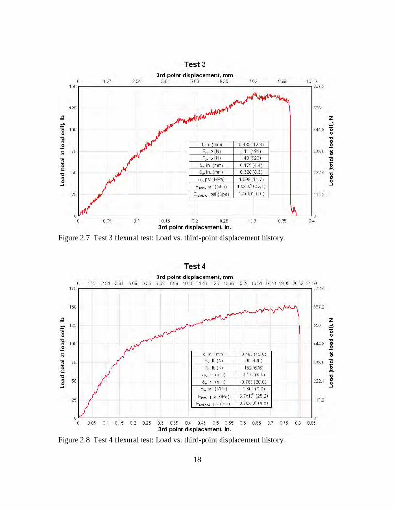
18
Figure 2.7 Test 3 flexural test: Load vs. third-point displacement history.
Figure 2.8 Test 4 flexural test: Load vs. third-point displacement history.
19
Figure 2.9 Test 5 flexural test: Load vs. third-point displacement history.
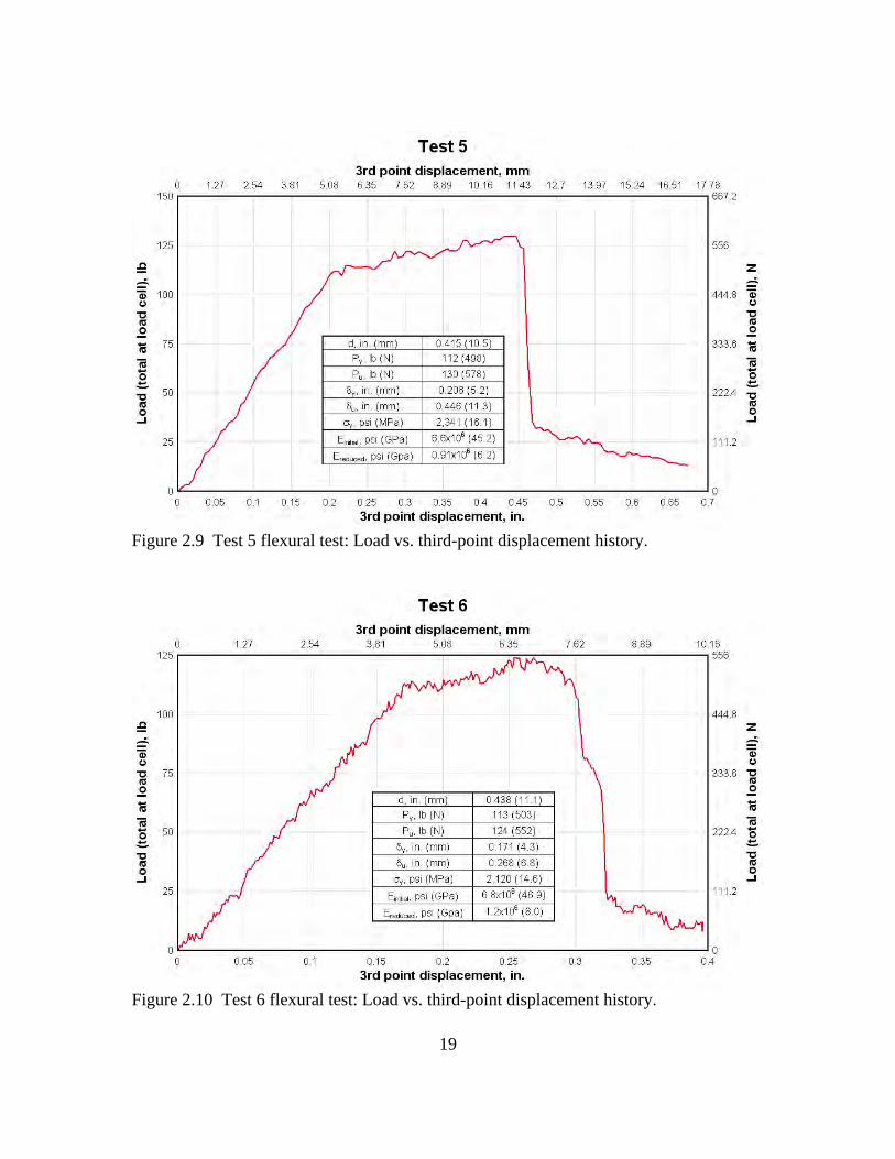
Figure 2.10 Test 6 flexural test: Load vs. third-point displacement history.

20
Figure 2.11 Test 7 flexural test: Load vs. third-point displacement history.
Figure 2.12 Test 8 flexural test: Load vs. third-point displacement history.

21
Figure 2.13 Test 9 flexural test: Load vs. third-point displacement history.
Figure 2.14 Test 10 flexural test: Load vs. third-point displacement history.

22
A cursory review of equation 1 shows that this is simply a form of the elastic
flexure formula [48], which carries the assumptions that over a differential specimen
length:
• At the location of consideration the section is subjected to pure bending and hence
curvature is constant.
• Plane surfaces through the section remain plane during bending.
• Stress and strain vary linearly through the section thickness.
• The material is homogeneous so that Hooke’s law of stress-strain proportionality
applies.
Since the point of consideration used to calculate first-crack strength was at the
panel third-point, the first assumption of pure bending was accepted. Furthermore, the
second and third assumptions are derived from basic structural mechanics, and were thus
also accepted. The fourth assumption of material homogeneity and corresponding
constant elastic modulus was assumed to be partially valid, depending on the scale of
consideration. Clearly the material was not truly homogeneous, and even from a
mesoscale viewpoint, it was composed of two distinctly different materials – namely the
hardened cementitous matrix and the AR glass fibers. However, at the macroscopic scale,
the cementitous matrix and glass fiber constituents could be homogenized into a uniform
material of quasi-homogeneous properties, and the fourth assumption was, therefore,
assumed to be satisfied.

23
Following acceptance of the fourth assumption from the elastic flexure formula,
the material’s initial flexural elastic modulus was calculated from the modulus of
elasticity equation given in ASTM C947-03, which states,
(2)
where,
Einitial = flexural elastic modulus during initial linear response, psi or MPa
δy = displacement at first-crack formation, in. or mm
The initial flexural modulus calculated from equation 2 is reported for each test
specimen in Figures 2.5 through 2.14.
Equations 1 and 2 describe the specimens’ initial linear response in a simple,
analytical sense; however, the specimens’ behavior – during both the initial and
post-crack responses – can also be considered in greater detail from a micromechanical
perspective. Prior to the point of first-crack formation (analogous to flexural yield in the
load-displacement plots), it can be assumed that the cementitious matrix and AR glass
fibers strained without damage, resulting in the initial linear response observed in all
tests. However, at the point of supposed flexural yield, the strain capacity of the cemen-
titous matrix was exceeded, and microcrack formation began to take place throughout the
area of maximum strain in the specimen. The microcracks initially formed at natural
flaws randomly distributed throughout the matrix, and therefore can be considered (at
formation) as local, unconnected damage points following the same stochastic distribu-
tion as the flaws. As the load increased, the microcracks grew and coalesced into larger,
more extensive damage areas. However, the randomly distributed glass fibers also
)27/()5( 33 bdLPE yyinitial δ=

24
provided a resistance to the microcrack growth, and the combined effect of the two
resulted in the observed response between first-crack and ultimate loads – characterized
by a sharp drop in the specimen stiffness and its resistance to the applied load. Finally,
after formation, growth, and full coalescence of the microcracks, a single large macro-
crack formed through the specimen cross section. With formation of the large macro-
crack, the specimens’ resistance to load rapidly diminished and finally resulted in failure
of the specimen. In Tests 5, 6, 8, and 9, a small residual load capacity was observed after
the macrocrack formation. This residual capacity was a result of glass fiber bridging
across the macrocrack during the final stages of fiber failure. The fact that this residual
capacity was not observed for the other specimens is indicative of the randomly dispersed
fibers’ stochastic nature, where the concentration of bridging fibers was likely not as
great in the area of the crack and, hence, the residual capacity was not developed.
Considering in further detail the stiffness loss between first-crack and ultimate
loads, a generic definition of stiffness as the product of flexural modulus and moment of
inertia (or E×I) is adopted. From this definition, it is seen that the stiffness loss occurring
after the first-crack point must largely be the effect of either a decrease in modulus or a
decrease in moment of inertia. A decrease in flexural modulus is taken to be the cause,
and the first argument for this assertion is based on observations of macrocrack formation
in each of the specimens. In each test, formation of a single macrocrack coincided with
the point of ultimate load, after which panel resistance rapidly decayed. Taking
macrocrack formation as the mechanism by which the specimens’ moment of inertia
would be reduced, the results show that between the first-crack and ultimate loads, the

25
specimens’ moment of inertia did not effectively change at the macroscopic level.
However, from the preceding discussion of micromechanical material behavior, it has
already been noted that damage growth, at the micro- and mescoscale levels, should be
expected between the points of first-crack and ultimate load. Although at fine length
scales this damage growth represents complex fracture and crack growth phenomena,
over the gross cross section the net effect can be homogenized into a basic descriptive
parameter. Assuming this parameter to be the flexural modulus, the loss of global stress-
strain resistance as a result of damage accumulation at the micro- and mesoscale levels
can be described through a modulus reduction. Therefore, through this argument of sub-
macroscale damage homogenization, the notion of flexural modulus reduction as the
cause of stiffness loss between first-crack and ultimate loads is further accepted.
It is interesting to note that although the microcrack damage to the concrete
specimen was in a state of growth between the first-crack and ultimate loads, the
reduction in global stiffness was generally constant—as evidenced by the generally linear
slope of the post-crack load-displacement curves. This indicates that the damage which
occurred during, and immediately after, initial microcrack formation caused an initial loss
of global stiffness, but the subsequent microcrack growth did not have a significant
impact on response until full formation of a single macrocrack occurred and
corresponding total failure of the specimen took place.
Given the preceding arguments for microscale damage as the primary cause of
stiffness loss in the panels, and its consideration in a global, homogenized sense, the
fourth assumption of the elastic flexure equation (namely that of material homogeneity

26
and proportional stress-strain) is still taken as valid for the panel response between first-
crack and ultimate load. Therefore, a reduced flexural modulus can be calculated in the
same manner as the initial flexural modulus, as follows,
(3)
where,
Ereduced = reduced flexural modulus between first-crack and ultimate load, psi or MPa
Pu = ultimate load (measured at the load cell), lb or N
δu = displacement at ultimate load, in. or mm
The mechanical properties given in Figures 2.5 through 2.14 are also summarized
in Table 2.3. In the table, mean values and standard deviations have been calculated for
each property. Notably, small standard deviations were seen for the mean panel thickness
(d), first-crack load (Py), ultimate load (Pu), displacement at first-crack (δy), flexural
strength (σy), and initial elastic modulus (Einitial), with values less than approximately
20 percent of the mean in all cases. In contrast, significantly greater deviation was seen
for the displacement at ultimate load (δu) and for the post-crack modulus (Ereduced), with
magnitudes of 38 percent and 41 percent, respectively (expressed in terms of percent of
the mean). The increased variability in these parameters, with particular emphasis on the
displacement at ultimate load, is attributed to the random glass fiber dispersion in the
specimens, and its subsequent influence on the panel ductility.
])(27/[])(5[ 33 bdLPPE uyuyreduced δδ −−=

27
E red
uced
, psi
(G
Pa)
0.86
×106 (6
.0)
0.46
×106 (3
.2)
1.4×
106 (9
.9)
0.70
×106 (4
.8)
0.91
×106 (6
.2)
1.2×
106 (8
.0)
0.63
×106 (4
.3)
0.40
×106 (2
.7)
0.89
×106 (6
.1)
0.44
×106 (6
.1)
0.79
×106 (5
.4)
0.33
×106 (2
.3)
E ini
tial,
psi
(GPa
)
4.1×
106 (2
8.3)
5.9×
106 (4
0.9)
4.8×
106 (3
3.1)
3.7×
106 (2
5.2)
6.6×
106 (4
5.2)
6.8×
106 (4
6.9)
5.7×
106 (3
9.0)
6.4×
106 (4
4.1)
5.9×
106 (4
0.4)
7.0×
106 (4
0.4)
5.7×
106 (3
9.2)
1.1×
106 (7
.6)
σ y, p
si
(MPa
) 2,
144
(14.
8)
1,78
3 (1
2.3)
1,69
9 (1
1.7)
1,30
6 (9
.0)
2,34
1 (1
6.1)
2,12
0 (1
4.6)
1,92
0 (1
3.2)
1,57
8 (1
0.9)
1,79
8 (1
2.4)
2,17
9 (1
5.0)
1,88
7 (1
3.0)
316
(2.1
)
δ u, i
n. (m
m)
0.81
6 (2
0.7)
0.49
4 (1
2.5)
0.32
8 (8
.3)
0.78
8 (2
0.0)
0.44
6 (1
1.3)
0.26
8 (6
.8)
0.83
1 (2
1.1)
0.43
7 (1
1.1)
0.38
8 (9
.8)
0.61
2 (1
5.5)
0.54
1 (1
3.7)
0.20
8 (5
.3)
δ y, i
n.
(mm
) 0.
272
(6.9
)
0.13
7 (3
.5)
0.17
5 (4
.4)
0.17
2 (4
.4)
0.20
6 (5
.2)
0.17
1 (4
.3)
0.18
1 (4
.6)
0.12
3 (3
.1)
0.15
2 (3
.9)
0.17
2 (4
.4)
0.17
6 (4
.5)
0.04
1 (1
)
P u, l
b (N
)
179
(796
)
165
(734
)
140
(623
)
152
(676
)
130
(578
)
124
(552
)
151
(672
)
157
(698
)
168
(747
)
154
(685
)
152
(676
)
17 (7
6)
P y, l
b (N
)
126
(560
)
137
(609
)
111
(494
)
90 (4
00)
112
(498
)
113
(503
)
108
(480
)
101
(449
)
117
(520
)
113
(503
)
113
(502
)
13 (5
8)
d, in
. (m
m)
.460
(11.
7)
0.52
6 (1
3.4)
0.48
5 (1
2.3)
0.49
8 (1
2.6)
0.41
5 (1
0.5)
0.43
8 (1
1.1)
0.45
0 (1
1.4)
0.48
0 (1
2.2)
0.48
4 (1
2.3)
0.43
3 (1
1.0)
0.46
7 (1
1.8)
0.03
4 (0
.9)
Spec
imen
1 2 3 4 5 6 7 8 9 10
Mea
n
Stan
d.
devi
atio
n
Tabl
e 2.
3
Flex
ural
test
spec
imen
s, m
echa
nica
l pro
perti
es

28
To provide for direct comparison between the specimen responses, all of the
load-displacement histories were plotted on a single graph in Figure 2.15. From this
figure, it is again shown that the specimens exhibited reasonable uniformity in their initial
linear response, point of first-crack formation, and post-crack stiffness. Furthermore,
from the graph, it is also seen that the greatest variability, by far, in specimen response
was the ultimate displacement, with magnitude ranging from approximately 0.3 in.
(7.6 mm) to 0.9 in. (22.9 mm), or equivalently 60 percent to 180 percent of the specimen
thickness.
Figure 2.15 Flexural tests: Load-displacement history comparisons. In concluding support of the argument that the specimens’ wide range of ductility
was largely a result of the stochastically distributed fiber reinforcement, reference is
made to the crack formation process observed during testing. In most all cases, once the

29
applied load reached its maximum value, initiation of a single macrocrack was observed,
typically at a panel edge. After initial formation, the crack propagated across the
specimen, and a total loss of resistance coincided (or near total loss of resistance in the
case of Tests 5, 6, 8, and 9). However, in Test 7 a different mode of crack formation and
propagation was observed. In this test, which showed the greatest ultimate displacement,
as the specimen reached its maximum load, multiple cracks were initiated on the tension
face. These cracks, shown in Figure 2.16, included one major crack and several parallel,
finer cracks. This observation of simultaneous, multiple crack initiation was similar to the
well-documented response of engineered cementitous composites, or ECCs [25, 31,
35, 37].
In ECC, random fiber reinforcement is incorporated into the cementitous matrix
in an engineered manner so that after initiation of an initial crack, the bridging fibers
maintain adequate strength to allow the next weakest portion of the material to crack.
This cracking/bridging process continues until the material is saturated with numerous
fine, parallel cracks. The formation of these multiple cracks yields a response known as
quasi-strain hardening or pseudo-strain hardening, and results in significantly increased
ductility over the single crack condition.
In Test 7, fibers bridging across the initial crack provided sufficient resistance to
begin formation of adjacent cracks in the specimen. However, the fibers’ bridging
capability was not adequate to form the saturated crack condition, and, as seen in Figure
2.17, the specimen failed in a single crack mode. However, initiation of this fiber-driven,
multiple crack process indicates that the increased ductility seen in Test 7 was a result of

30
the fiber influence, and by extension the ultimate displacement variability observed in all
tests is attributed to the fiber influence.
Figure 2.16 Test 7, multiple crack initiation.
Figure 2.17 Test 7, final single crack failure.

31
From Figure 2.15, a load-displacement response envelope for the 0.5-in.-thick
(12.7-mm) panels was determined, and is shown in Figure 2.18. Furthermore, using the
mean physical and mechanical properties given in Table 2.3, an average response
function was computed and is also shown in the figure. As seen, the average response
function falls well within the envelope limits and closely matches the envelope’s pre- and
post-crack stiffness. Because of the large variability observed for ultimate displacement
in the specimens, an ultimate failure point is not shown. When using this function as a
predictive tool, it is expected that an assumption would be made regarding the ultimate
load and displacement capacity, and limits of the predictive function would be adjusted
accordingly. However, so that the ultimate failure point is not always required to be
known a priori, a numerical tool is developed in a subsequent chapter to calculate the
point of ultimate failure based on material properties.

32
Figure 2.18 Flexural test: Response envelope and mean response function.

33
CHAPTER III
DIRECT TENSION EXPERIMENTS In addition to the flexural tests used to characterize the panel’s bending response,
a limited set of direct tension tests was also conducted. In the direct tension experiments,
a novel specimen configuration and experimental procedure were used in a closed-loop
testing system to directly measure (a) the material’s initial, linear-elastic tensile modulus,
and (b) the material’s load versus crack opening relationship under a pure tensile load.
The tensile modulus measurement was used for validation of the modulus calculated from
the flexural tests, but of greater significance was direct measurement of the load versus
crack opening relationship after initial crack formation in the specimen.
As stated previously, the purpose for inclusion of the discontinuous reinforcing
fibers was improvement of the otherwise brittle material’s post-crack ductility when
exposed to a tensile load. Observed in the flexural experiments as post-crack hardening,
the fiber’s impact on bending response was an increase of maximum displacement from a
mean value of 0.176 in. (4.5 mm) at first-crack formation to a mean value of 0.541 in.
(13.7 mm) at ultimate failure. Although this increase in failure displacement was a result
of including fibers in the matrix, the measured bending response did not provide a direct
quantification of the fiber’s impact on response to tensile load. Rather, direct tension
experiments were required to explicitly measure the fiber’s influence on the material’s
post-crack softening behavior, which in turn could be used to further study the fiber

34
bridging mechanics (as done in the micromechanical analyses in Chapter IV) and could
also be used in development of numerical models (as done in the FE analyses in
Chapter V).
It is noted that based on limited resource availability, only a small number of
direct tension tests could be conducted in this experimental effort. However, the data
were expected to yield indicative results, which would provide support to other aspects of
the project as described above. Therefore, future research on the VHSC material should
consider additional direct tension tests, so that the presented data set could be further
populated and estimates of the post-crack ductility could be further refined.
3.1 Testing procedure and equipment
In contrast to the flexural experiments, which followed a published ASTM stan-
dard test method, standardized procedures were not available for design and execution of
the direct tension tests. In the literature, it is noted that a U.S. standard has not been
developed for this type of test, presumably because of the great difficulty in obtaining a
pure tensile loading condition. Furthermore, the convolution of strain localization in a
cracked concrete specimen further increases the difficulty in extracting meaningful strain
data from a test, which is also a likely cause for the lack of standardized tests of this type.
Although standard test methods were not available, research pertaining to
concrete direct tension tests has been documented [49, 50]. From these works, the
approach and procedures used for these tests were developed so that they would
reasonably follow other published efforts.

35
The loading machine used for testing was the same MTS machine used for the
flexural tests. The loading fixture used in the flexural tests was removed, and a new
fixture with a sleeve and pin connection was attached. The same type of sleeve and pin
fixture was connected to an anchor at the bottom of the MTS machine, and was aligned
with the fixture in the loading head. With the fixtures in-place and aligned, the test
specimens were placed in the machine and connected to the fixtures at each end so that a
direct tensile load could be applied.
Review of the literature revealed that three general testing criteria should be
satisfied to obtain the most meaningful direct tension data, and these included:
• Application of load without eccentricity to the specimen, such that a pure tensile
loading condition is achieved.
• Sufficient rigidity in the testing apparatus so that as the crack opens, it does so
uniformly across the width of the specimen.
• Sufficient stiffness in the closed-loop system so that after fracture of the
specimen, the post-crack response can be recorded.
From these criteria, a great deal of the difficulty associated with direct tension
tests arises, due to the fact that means of resolution for one can prevent satisfaction of the
other. To provide an example, a method used in the past to minimize loading eccentricity
was to connect the specimen to the test machine with chains (or alternatively, cable could
also be used). The flexible chain or cable would provide rotational degrees of freedom
between the machine and the specimen so that if the loading fixtures were not perfectly
aligned, they would not induce a bending load. Although this satisfies the first criterion

36
given above, on macrocrack initiation (typically beginning at one side of the specimen) a
new loading eccentricity is developed, and a non-uniform crack opening width occurs.
An example of this is shown in Figure 3.1, in which a specimen was connected to
the machine with chains. As seen, the crack opening width is very non-uniform, and it is
not possible to resolve either the stress or strain at the cracked section. In turn,
meaningful information cannot be obtained with regard to the specimen’s post-crack
response. The means of resolution to the non-uniform crack opening is to provide very
rigid connections to the testing machine, which force displacement at the crack to be
uniform across the specimen width. However, the drawback to this test configuration is
that if the specimen and test fixtures are not in perfect alignment, then an uncontrolled
bending load will be applied to the specimen. This, of course, also convolutes data
obtained from the tests, and should be avoided as well.
Figure 3.1 Direct tension test, non-uniform crack opening.

37
Recognizing the above requirements and implications arising from each, tests in
this study were conducted with a rigid connection between the specimen and fixture so as
to minimize the potential for a non-uniform crack opening at the cracked section. This
was considered to be the required approach because, although uncontrolled bending
might be induced in the specimen, without fixture rigidity, meaningful post-crack data
could not be obtained.
A test specimen mounted in the machine, with rigid connections to the loading
fixtures, is shown in Figure 3.2.
Figure 3.2 Direct tension specimen with rigid connection to fixture.
38
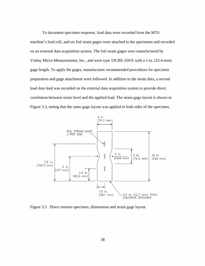
To document specimen response, load data were recorded from the MTS
machine’s load cell, and six foil strain gages were attached to the specimens and recorded
on an external data acquisition system. The foil strain gages were manufactured by
Vishay Micro-Measurements, Inc., and were type 10CBE-350/E with a 1-in. (25.4-mm)
gage length. To apply the gages, manufacturer recommended procedures for specimen
preparation and gage attachment were followed. In addition to the strain data, a second
load data feed was recorded on the external data acquisition system to provide direct
correlation between strain level and the applied load. The strain gage layout is shown in
Figure 3.3, noting that the same gage layout was applied to both sides of the specimen.
Figure 3.3 Direct tension specimen, dimensions and strain gage layout.

39
3.2 Tension test specimens
In the same manner as done for the flexural tests, specimens used in the direct
tension tests were cut from larger, nominally 0.5-in.-thick (12.7-mm) panels on a
water-jet cutting machine. Taking the test specimens from larger panels in this fashion
helped ensure that the documented responses would most accurately represent that of
full-sized production panels.
To control the location of crack formation, the specimens were cut in a notched
shape, somewhat analogous to the typical dog-bone shape used in steel coupon tensile
tests. However, to ensure that the 1-in.-long (25.4-mm) strain gages would be located at
the crack and thereby capture the load versus crack opening response, instead of the long
necked down section used in steel tests, these tests utilized a sharp v-notch shape.
Dimensions of the specimen and the v-notch are also shown in Figure 3.3, in conjunction
with the strain gage layout.
From the literature, it was determined that the preferred way to mount the
specimens into the test machine was by use of steel end caps. Use of end caps, epoxied to
the specimen ends, allowed for dissipation of the stress concentration that occurred at the
connection point. Resultantly, the load applied at the specimen end was expected to be a
uniform stress over the cross section. The steel end caps were 3-in. (76.2-mm) wide, 4-in.
(101.6-mm) long, and 0.5-in. (12.7-mm) thick, and had a threaded receiver to provide for
connection to the MTS machine. The caps were epoxied to the specimens with Sika Dur
31 Hi-Mod epoxy, which has published modulus and tensile strength of 1.7×10⁶ psi
(11.5 GPa) and 3,300 psi (22.7 MPa), respectively. A mold was built for attachment of

40
the caps and specimens to minimize misalignment between the two. A specimen placed
inside the mold, with steel caps on each end, is shown in Figure 3.4.
Figure 3.4 Direct tension specimen with epoxied steel end caps. 3.3 Experimental results
Four tests were conducted as a part of the direct tension experiments, with
specimens prepared, strained, and monitored as previously described. In the third test, the
specimen failed prematurely at an end cap connection by delamination of a thin mortar
layer adhered to the epoxy. For this reason, results from the third test were discarded,
leaving three data sets for analysis.

41
Observation of the crack formation and propagation at the notched section
showed that the rigid test fixture connections resulted in a generally uniform crack
opening—providing significant improvement over the lack of crack opening uniformity
seen with rotationally free connections (reference Figure 3.1). As an example of this, the
cracked specimen at completion of Test 1 is shown in Figure 3.5.
Figure 3.5 Tension Test 1, cracked specimen at test completion.
A test data set was comprised of six strain-load histories recorded at the six strain
gages. Recalling that three strain gages were attached to each side of the specimen, gage
notation was established so that gages on the specimen front face (as mounted in the
MTS machine) were labeled “A” gages, and those on the back were labeled “B” gages.
Furthermore, on each side the gages were numbered 1 through 3, with the gage at the top

42
being labeled 1, the gage at the center labeled 2, and the gage at the bottom labeled 3. In
this manner, all gages were given unique identifiers that were used for data identification.
As an example, gage designations A1 through A3 on the specimen front face in Test 1 are
shown in Figure 3.6. Gages on the back face of this specimen were similarly designated
B1, B2, and B3, with B1 located at the top.
Figure 3.6 Tension test strain gage designations, “A” side.
The recorded load versus strain histories are given in Figures 3.7 through 3.9,
3.10 through 3.12, and 3.13 through 3.14 for Tests 1, 2, and 4, respectively. Typical sign
convention was adopted for the test data, where tensile strains were denoted by positive
values and compressive strains by negative. Note that the data are presented in load-strain
history format, which is how it was recorded, instead of stress-strain history as might be

43
typically expected. Load data were not immediately converted to corresponding stress
due to uncertainty in stress states at the gages, but is given later after further analysis.
Figure 3.7 Tension Test 1: Load-strain history, gage A1 vs. gage B1.

44
Figure 3.8 Tension Test 1: Load-strain history, gage A2 vs. gage B2.
Figure 3.9 Tension Test 1: Load-strain history, gage A3 vs. gage B3.

45
Figure 3.10 Tension Test 2: Load-strain history, gage A1 vs. gage B1.
Figure 3.11 Tension Test 2: Load-strain history, gage A2 vs. gage B2.

46
Figure 3.12 Tension Test 2: Load-strain history, gage A3 vs. gage B3.
Figure 3.13 Tension Test 4: Load-strain history, gage A1 vs. gage B1.

47
Figure 3.14 Tension Test 4: Load-strain history, gage A2 vs. gage B2.
From the load-strain data, it was immediately observed that all three specimens
experienced bending-induced strains. This was evidenced by the initial tension and
compression strain coupling measured at each of the strain gage pairs (i.e. A1-B1, A2-
B2, and A3-B3). As the load levels increased, the bending-induced compressive strains
were overcome by the pure tensile strains, and the entire section was transitioned into a
fully tensile strain state. This is not to say that the bending strain state disappeared once
the entire section was in tension. Rather, the compressive strains were masked by pure
tensile strains of greater magnitude as the loads increased. The bending strains are known
to be present through the point of maximum load by observation that even with the full
cross section in tension, the strain states on the front and back faces were not equal. For
example, in Test 1, side A of the specimen was initially strained in tension and side B in
compression, with maximum compression of approximately 28 microstrains reached at a

48
load of 103 lb (458 N). The pure tension strains worked to overcome the compression
strains up to a load of approximately 430 lb (1,913 N), at which point the entire section
was strained in tension. Although the entire cross section was strained in tension at loads
above 430 lb (1,913 N), the strain magnitude at gage A1 remained much higher than at
B1 for the loading duration. Had the bending strains been relieved, the strain magnitude
at A1 and B1 should have been equal. However, their observed inequality gives evidence
for continuance of the bending strain state.
The expected cause of the bending state was minor misalignment of the threaded
connections on the steel end caps. The threaded connections, shown in Figure 3.15, were
welded to pieces of bar stock to form the end caps. Care was taken during the welding
process to center the threaded connection on the bar, but measurements showed that small
deviations were still present in the connectors’ exact location on each cap. This caused
the load centroid to have eccentricity with respect to the specimen centroid, which
resulted in the observed bending conditions.
Figure 3.15 Tension test end cap, threaded connector welded to bar stock.
49
3.4 Elastic strain state analysis
Although the specimens were strained in a complex state, review of the data still
provides a clear understanding of the specimens’ global response to the loads. Until the
point of maximum load, each gage measured a generally linear strain gradient with load
increase, verifying material linearity during pre-crack response. At the point of maximum
load, the notched section (gages A2 and B2) began to show significant increases in strain,
while gages at the ends (A1, B1, A3, and B3) showed strain recovery. This observation of
strain increase at one section and strain recovery at another exactly describes the concept
of strain localization in brittle materials, in that as microcracks formed and coalesced at
the notched section, they allowed for relief of strain throughout other portions of the
specimen. Eventually, a macrocrack was formed at the notch and grew until failure, while
remaining portions of the specimen experienced complete strain recovery. Because the
specimens’ end sections experienced this full recovery of strain, the data showed that not
only was the material’s pre-crack response generally linear, it was also near fully elastic –
with little material damage occurring until rapid microcrack formation and localization
began.
Because the specimens were in a combined state of bending and pure tension
strain during the tests, the data could not be immediately used to determine the initial
tensile modulus, which was desired for comparison to the flexural tests. This was due to
the fact that without quantification of the bending moment experienced by the specimen,
the true stress state could not be determined at the gage locations. Without the stress state
50
corresponding to the measured strains, subsequent calculation of the modulus could not
be performed.
To rectify the stress state ambiguity, first the strain data were analyzed to separate
it into strains resulting from the pure tensile load and strains resulting from the moment
induced bending. With measured strains resolved into these two components, the applied
load and specimen cross-sectional areas could be used to calculate the pure tension stress,
which coupled with the pure tension strain would yield the true tensile modulus of the
material.
Referencing the free-body diagram shown in Figure 3.16, a load, P, applied with
eccentricities e1 and e2 results in a uniform tensile stress over the cross section, σ1, and a
bending moment, Mr. The bending moment, Mr, can be expressed as the sum of
individual bending moments, M1 and M2, which are calculated as:
(4)
(5)
and the uniform stress due to the pure tension load, σ1, can be expressed as,
(6)
where A denotes the cross-sectional area of the specimen at the point of interest.
Further referencing the free-body diagrams given in Figure 3.17 and Figure 3.18, which
describe the strain states occurring when the cross section is strained in either combined
tension and compression or tension only, it is seen that the measured strains at the
specimen face, εtens and εcomp (or εtensmax and εtensmin for the tension only condition), can be
expressed as the sum of strains resulting from the pure tension load, ε1, and strains
11 PeM =
22 PeM =
AP=1σ

51
resulting from the bending load, ε2. Making the assumption that the cross section has not
cracked and is behaving as a quasi-homogeneous, linear-elastic material, the bending
strains can be assumed symmetric about the cross section’s neutral axis, which is located
one-half of the section thickness, t, from each face.
Figure 3.16 Tension specimen free body diagram.
Figure 3.17 Tension specimen, strain resolution with tension and compression strain
state.
Figure 3.18 Tension specimen, strain resolution with tension only strain state.

52
The final assumption that must be accepted before resolution of the cross section
strains can be made is that the strain gradient through the cross section due to combined
bending and tension is the same as the strain gradient due to bending only. Otherwise
stated, the strain gradient resulting from the measured strains, εtens and εcomp (or εtensmax
and εtensmin), is the same as the gradient between the pure bending strains, ε2, at each face
of the specimen. The pure tension strain, ε1, simply acts as a uniform shift of the tension
and compression strain magnitudes on the cross section, but does not change the slope of
the linear strain distribution. Acceptance of this assumption indicates that the strain
distribution over the cross section and the strain distribution due to pure bending are
geometrically similar, resulting in the equations,
(7)
which can be rearranged as,
(8)
and,
(9)
which can be rearranged as,
(10)
Knowing that εtens is the summation of ε1 and ε2, equation 11 can be written, which is
solved by use of the measured tensile strains, εtens, and the bending strain computed in
equation 10.
(11)
xtxtenscomp
−=
εε
tenscomp
comp tx
εεε
+=
xtttens
−=
εε5.02
)1(5.02 xtt tens −
= εε
21 εεε −= sten

53
The strain computed from equation 11, ε1, is the portion of the measured strain that is a
result of the pure tension load and corresponding tensile stress, σ1.
By the same arguments used to write equations 7 through 10, a new equation can
be written for the strain state shown in Figure 3.18,
(12)
which can be rearranged as,
(13)
Using equation 11 (substituting εtensmax for εtens) and the bending strain computed
in equation 13, the strain from pure tension, ε1, can also be computed for this strain state.
Resolution of the bending and tension strains for Tests 1, 2, and 4 are given in
Table 3.1, Table 3.2, and Table 3.3, respectively. At selected load levels, measured
strains were pulled from the data, and from these the neutral axis location, x, bending
strain, ε2, and pure tension strain, ε1, were calculated. The pure strain data were then
plotted against the measured strain-load histories in Figures 3.19 through 3.26. As seen,
with exception of the A2, B2 gage pair in Test 2, the pure tension strains were resolved to
a straight line, as should have been expected during the pre-crack specimen response.
Note that this observation of linearity in strain-load space is in agreement with
conclusions drawn from the flexural experiments, where it was also observed that the
initial material response was linear in nature.
tttenten minmax2
5.0εεε −
=
)(5.0 minmax2 tensten εεε −=

54
Table 3.1
Direct tension Test 1, elastic strain analysis
P, lb (N) εtens or εtensmax εcomp or εtensmin x, in. (mm) ε2 ε1
A1, B1 Average section thickness, t, = 0.5040 in. (12.8 mm) 60 (266.9) 0.00003546634 0.00002230496 0.195 (4.9) 0.00002888565 0.00000658069 97.5 (434) 0.00005155328 0.00002778994 0.176 (4.5) 0.00003967161 0.00001188167 225 (1001) 0.00006733617 0.00001654470 0.099 (2.5) 0.00004194044 0.00002539574 375 (1668) 0.00008738130 0.00000333617 0.018 (0.4) 0.00004535874 0.00004202257 428 (1904) 0.00009176821 0.00000000000 0 0.00004588411 0.00004588411 600 (2667) 0.00011297110 0.00001755069 - 0.00004771021 0.00006526090 750 (3336) 0.00013124860 0.00003254138 - 0.00004935361 0.00008189499 900 (4003) 0.00014839700 0.00004614468 - 0.00005112616 0.00009727084
1050 (4670) 0.00016341530 0.00006401281 - 0.00004970125 0.00011371406 A2, B2 Average section thickness, t, = 0.5132 in. (13.0 mm)
50 (222) 0.00003217576 0.00001682003 0.176 (4.5) 0.00002449790 0.00000767787 100 (448) 0.00005372465 0.00002705860 0.172 (4.4) 0.00004039163 0.00001333303
250 (1112) 0.00007019882 0.00001096952 0.069 (1.7) 0.00004058417 0.00002961465 360 (1601) 0.00008262876 0.00000000000 0 0.00004131438 0.00004131438 500 (2224) 0.00010090750 0.00001608816 - 0.00004240967 0.00005849783 600 (2669) 0.00011187440 0.00002559454 - 0.00004313993 0.00006873447 700 (3114) 0.00012430320 0.00003583196 - 0.00004423562 0.00008006758 800 (3558) 0.00013965600 0.00004972525 - 0.00004496538 0.00009469063
1000 (4448) 0.00017258060 0.00006451613 - 0.00005403224 0.00011854837 1100 (4893) 0.00018936640 0.00007093000 0.00005921820 0.00013014820 A3, B3 Average section thickness, t, = 0.5175 in. (13.0 mm)
50 (222) 0.00002351064 0.00001039894 0.159 (4.0) 0.00001695479 0.00000655585 100 (445) 0.00003401601 0.00001034628 0.121 (3.1) 0.00002218115 0.00001183487 150 (667) 0.00003767217 0.00000358168 0.045 (1.1) 0.00002062693 0.00001704525 180 (801) 0.00003922872 0.00000000000 0 0.00001961436 0.00001961436
300 (1334) 0.00005032258 0.00001580645 - 0.00001725807 0.00003306452 450 (2002) 0.00006435484 0.00003209677 - 0.00001612904 0.00004822581 600 (2667) 0.00008032258 0.00004935484 - 0.00001548387 0.00006483871 750 (3336) 0.00009612903 0.00006500000 - 0.00001556452 0.00008056452 900 (4003) 0.00011131800 0.00008084845 - 0.00001523478 0.00009608323
1100 (4893) 0.00013177100 0.00010463860 - 0.00001356620 0.00011820480

55
Table 3.2
Direct tension Test 2, elastic strain analysis
P, lb (N) εtens or εtensmax εcomp or εtensmin x, in. (mm) ε2 ε1
A1, B1 Average section thickness, t, = 0.5460 in. (13.9 mm)
40 (178) 0.00001627660 0.00000627660 0.152 (3.9) 0.00001127660 0.00000500000 100 (448) 0.00003340426 0.00001148936 0.140 (3.6) 0.00002244681 0.00001095745 200 (890) 0.00005117021 0.00000755319 0.069 (1.8) 0.00002936170 0.00002180851
300 (1334) 0.00006372340 0.00000000000 0 0.00003186170 0.00003186170 450 (2002) 0.00008418782 0.00001187234 - 0.00003615774 0.00004803008 600 (2669) 0.00010593930 0.00002137885 - 0.00004228023 0.00006365908 750 (3336) 0.00012620970 0.00003112903 - 0.00004754034 0.00007866937 900 (4003) 0.00014677420 0.00004148813 - 0.00005264304 0.00009413117 1050 (4670) 0.00017048390 0.00005072581 - 0.00005987905 0.00011060486
A2, B2 Average section thickness, t, = 0.5260 in. (13.4 mm)
60 (267) 0.00003583196 0.00002267062 0.204 (5.2) 0.00002925129 0.00000658067 120 (534) 0.00006288693 0.00003364066 0.183 (4.6) 0.00004826380 0.00001462314 200 (890) 0.00008043526 0.00002852128 0.138 (3.5) 0.00005447827 0.00002595699 350 (1557) 0.00009798294 0.00000000000 0 0.00004899147 0.00004899147 500 (2224) 0.00011260550 0.00007824176 - 0.00001718187 0.00009542363 600 (2667) 0.00016012570 0.00011626110 - 0.00002193230 0.00013819340
A3, B3 Average section thickness, t, = 0.5245 in. (13.3 mm)
60 (267) 0.00003290701 0.00001499174 0.164 (4.2) 0.00002394938 0.00000895764 120 (534) 0.00005484525 0.00002687577 0.174 (4.4) 0.00004049415 0.00001361838 200 (890) 0.00006727407 0.00002167556 0.128 (3.2) 0.00004447482 0.00002279926
400 (1779) 0.00009278549 0.00000603320 0.032 (0.8) 0.00004940935 0.00004337614 490 (2180) 0.00010495200 0.00000000000 0 0.00005247600 0.00005247600 600 (2669) 0.00012032260 0.00001078644 - 0.00005476808 0.00006555452 750 (3336) 0.00014111820 0.00002135484 - 0.00005988168 0.00008123652 900 (4003) 0.00016085670 0.00003225806 - 0.00006429932 0.00009655738 1050 (4670) 0.00018546240 0.00004288172 - 0.00007129034 0.00011417206

56
Table 3.3
Direct tension Test 4, elastic strain analysis
Figure 3.19 Tension test 1, elastic strain correction, gages A1 and B1.
P, lb (N) εtens or εtensmax εcomp or εtensmin x, in. (mm) ε2 ε1
A1, B1 Average section thickness, t, = 0.4930 in. (12.5 mm) 100 (444.8) 0.00005995731 0.00003573768 0.184 (4.7) 0.00004784750 0.00001210982 200 (889.6) 0.00009230591 0.00004597665 0.164 (4.2) 0.00006914128 0.00002316463 300 (1334) 0.00010290750 0.00003524013 0.126 (3.2) 0.00006907382 0.00003383369 400 (1779) 0.00011277770 0.00002563501 0.091 (2.3) 0.00006920636 0.00004357135 500 (2224) 0.00012155110 0.00001123821 0.042 (1.1) 0.00006639466 0.00005515645 570 (2535) 0.00012484100 0.00000000000 0 0.00006242050 0.00006242050
A2, B2 Average section thickness, t, = 0.4925 in. (12.5 mm) 100 (444.8) 0.00024126430 0.00009471196 0.139 (3.5) 0.00016798813 0.00007327617 200 (889.6) 0.00042541880 0.00013091970 0.116 (2.9) 0.00027816925 0.00014724955 300 (1334) 0.00054266990 0.00012909090 0.095 (2.4) 0.00033588040 0.00020678950 400 (1779) 0.00066500340 0.00012214180 0.076 (1.9) 0.00039357260 0.00027143080 500 (2224) 0.00080738120 0.00011336410 0.061 (1.5) 0.00046037265 0.00034700855 570 (2535) 0.00094387700 0.00011007250 0.051 (1.3) 0.00052697475 0.00041690225

57
Figure 3.20 Tension test 1, elastic strain correction, gages A2 and B2.
Figure 3.21 Tension test 1, elastic strain correction, gages A3 and B3.

58
Figure 3.22 Tension test 2, elastic strain correction, gages A1 and B1.
Figure 3.23 Tension test 2, elastic strain correction, gages A2 and B2.

59
Figure 3.24 Tension test 2, elastic strain correction, gages A3 and B3.
Figure 3.25 Tension test 4, elastic strain correction, gages A1 and B1.

60
Figure 3.26 Tension test 4, elastic strain correction, gages A2 and B2.
At the A2/B2 gage pair in Test 2, the load-strain path did not follow the same
pattern seen for all other locations. Initially, gage A2 was in compression and B2 was in
tension, showing the typical bending response. However, after transition into a complete
tension state over the entire cross section, gage A2 showed a rapid increase in tensile
strain while B2 showed much more gradual increases. The result of this was crossing of
the load-strain curves, implying a reversal of the bending direction. The probable cause
was that the after transitioning from compression to tension, the A2 side incurred
localized damage as a result of material heterogeneity, and it effectively yielded in
tension. This yielding caused initiation of bending compressive strains in the B2 side,
which decreased the rate of tensile strain growth and resulted in the observed response. In
consideration of this localized failure and bending reversal, the elastic pure tension
strains were only computed to the point of strain reversal.

61
An interesting observation made from overlaying the pure tension, linear-elastic
strain curves with the measured strains was that for the A1/B1 and A3/B3 gage pairs,
during their strain recovery portion of response, the recovery curves tended towards the
computed linear-elastic curve. This implies that once the specimens began to crack at the
notch, a hinge formed and worked to relieve the specimens’ bending strains. With
reduction of the bending strains, the only remaining strain in the specimens were those
caused by the pure tension load, and therefore the recovery curves migrated towards the
pure tension curve. Observation of this alignment between the computed pure tension
curve and the strain recovery curves validated the tension curves accuracy, along with the
procedure derived for their calculation.
3.5 Elastic stress state analysis and tensile modulus calculation
Before calculating the tensile modulus, a finite element (FE) analysis was
conducted to analyze the stress state within the specimen as a function of the applied
load. At a minimum, the FE analysis was required to determine the stress state at the
A2/B2 gage location because of the notch and resulting stress concentration.
Furthermore, the same analysis could be used to validate stress states at the A1/B1 and
A3/B3 locations, which would otherwise be calculated as load, P, divided by cross-
sectional area, A.
The program used for the FE analysis was ABAQUS/CAE, Version 6.5-4 [51].
ABAQUS is available in implicit and explicit versions, and can perform linear and
nonlinear calculations (nonlinear with respect to geometry and material properties) within
a Lagrangian framework. The implicit version was used for these calculations.

62
The FE model was built with two basic parts, which included the steel end caps
and the VHSC specimen. For modeling purposes, the specimen and end cap geometry
were based on the exact design dimensions, resulting in a model specimen thickness of
exactly 0.5 in. (12.7 mm). Although all experimental specimens showed small deviation
from the nominal 0.5-in. (12.7-mm) thickness, use of this assumed value in the FE model
remained valid because, as will be seen, FE results were used to determine the ratio
between actual stress and that calculated by P/A, which could in turn be applied to the
experimental data.
The model was meshed with linear, 8-noded hexahedral elements (ABAQUS
element type C3DR8), which possessed 3 degrees of freedom per node. Five elements
were provided through the specimen thickness, resulting in an element thickness of
0.1 in. (2.5 mm). The ABAQUS automatic mesh generator was used to build the mesh,
and along with thickness of 0.1 in. (2.5 mm), remaining element dimensions were
specified to be approximately 0.1 in. (2.5 mm). From model diagnostics, the minimum
and maximum angles between element faces were 71 degrees and 108 degrees,
respectively. The maximum aspect ratio between element face dimensions was 2.06. The
mesh contained 26,390 elements, 32,940 nodes, and 98,820 degrees of freedom (degrees
of freedom calculated prior to application of boundary conditions). The meshed model is
shown in Figure 3.27, with the end caps in red and the VHSC specimen in blue.

63
Figure 3.27 Tension test FE model.
Load was applied to the model as uniform pressure, distributed over a pair of
0.1-in.-wide (2.5-mm) strips at the top end cap. This was done to simulate the connection
between the threaded fastener welded to the end cap (which was not included in the
model) and the bar stock portion of the cap. External boundary conditions were applied to
the bottom end cap over similar 0.1-in.-wide (2.5-mm) strips, again simulating
connection between the end cap and threaded fastener. The applied loads are shown in
Figure 3.28, along with a picture of the welded connection between a threaded fastener
and the bar stock.

64
Figure 3.28 Tension test: FE load application.
Because characterization of the specimens’ stress distribution during initial elastic
response was the FE model’s primary function, the end caps and VHSC specimen were
both modeled with a simple isotropic, elastic material model. The selected material model
required only Young’s modulus and Poisson’s ratio, which were specified as 29×106 psi
(199.9 GPa) and 0.29 for the steel end caps, and 5.7×10⁶ psi (39.3 GPa) and 0.23 for the
VHSC specimen. The value of Poisson’s ratio for VHSC was taken from a prior ERDC
study [52] on similar material.
To perform the implicit calculation, an iterative solver was used with calculations
performed at specified increments of load such that stress versus load curves could be
developed. The maximum applied pressure was 11,000 psi (75.8 MPa), which equated to
1,100 lb (4,893 N) when applied over the specified area. Calculations were performed at
1,100 psi (7.6 MPa) pressure increments, or equivalent load increments of 110 lb
(489 N).

65
A contour plot of the axial stress component from the computed stress tensor at a
load level of 1,100 lb (4,893 N) is shown in Figure 3.29. In the plot, the contour range is
limited to a maximum value of 4,750 psi (32.8 MPa), so that greater fidelity is provided
over the range of interest. As a result, stresses greater than this are plotted in white. From
the figure, it is immediately observed that as a result of (a) specimen geometry,
(b) loading geometry, and (c) connection of the dissimilar materials, stress distribution
throughout the specimen is not perfectly uniform. As expected, at the point of load
application, a large stress gradient is present in the end cap. The gradient is generally
dissipated through the cap length, but at connection to the VHSC specimen, stresses still
range from approximately 830 psi ( 5.7 MPa) at the edge to 700 psi (4.8 MPa) at the
center. Based on cross-section dimensions of 0.5 in. (12.7 mm) by 3 in. (76.2 mm), at a
load of 1,100 lb (4,893 N), the nominal computed stress (by P/A) in the end cap would be
733 psi (5.0 MPa). Similar stress gradient is also seen at the A1 gage location. Stresses
range from approximately 830 psi (5.7 MPa) to 700 psi (4.8 MPa), but in this case the
higher stresses are located at the specimen center (in contrast to the steel end cap, where
stresses were greater at the edge). Lastly, at the A2 gage location, it is interestingly noted
that a very significant stress gradient is present. As expected, stress concentrations exist
at the notches, with magnitude of approximately 1,975 psi (13.6 MPa). However, the
large stress zone of approximately 1,025 psi (7.1 MPa) immediately adjacent to the
notches tends to flow or arch around the center of the notched section, resulting in a
stress level of approximately 890 psi (6.1 MPa) at the A2 gage location. Considering that
the stress at A2 would have been nominally calculated (by P/A) as 1,100 psi (7.6 MPa),

66
the FE results show that the stress level differed by as much as 19 percent from the
expected value. This will be of significance in using the A2 data for calculation of the
tensile modulus.
Figure 3.29 Tension test: FE axial stress contours at 1,100 lb (4,893 N) load.
To provide additional data at the A1 and A2 gage locations, load-stress histories
from the FE analysis are given in Figures 3.30 and 3.31, along with the stresses
nominally calculated by P/A. As seen from the graphs, at the A1 location the FE
calculated stress differed slightly from the nominal, with magnitude of approximately
5 percent greater than expected. However, at the A2 location the deviation was reversed.

67
In this case, at the strain gage location the FE stress was less than expected, with a
deviation of approximately 19 percent.
Figure 3.30 Tension test: Gage A1 FE and nominal stress-load histories.

68
Figure 3.31 Tension test: Gage A2 FE and nominal stress-load histories.
Using the information from Figures 3.30 and 3.31 as a correlation between
nominal stresses, σ1, and true stresses, σtrue, corrected stresses were calculated for the
load levels given in Tables 3.1 through 3.3. These corrected stresses are given in
Tables 3.4 through 3.6, along with the previously calculated pure tension strains, ε1. With
these data, the resulting tensile modulus, Edirecttension, was calculated from equation 14,
and is also given in Tables 3.4 through 3.6.
(14)
1εσ true
iondirecttensE =

69
Table 3.4
Direct tension Test 1, elastic stress analysis and tensile modulus calculation
P, lb (N) σ1, psi (MPa)
Correction factor
σtrue, psi (MPa) ε1
Edirecttension, psi (GPa)
A1, B1 Average section thickness, t, = 0.5040 in. (12.8 mm)
60 (266.9) 39.7 (0.27) 1.05 41.7 (0.29) 0.00000658069 6.34x10⁶ (43.7) 97.5 (434) 64.5 (0.44) 1.05 67.7 (0.47) 0.00001188167 5.70x10⁶ (39.3) 225 (1001) 148.8 (1.0) 1.05 156.2 (1.1) 0.00002539574 6.15x10⁶ (42.4) 375 (1668) 248.0 (1.7) 1.05 260.4 (1.8) 0.00004202257 6.20x10⁶ (42.7) 428 (1904) 283.1 (2.0) 1.05 297.2 (2.0) 0.00004588411 6.48x10⁶ (4.47) 600 (2667) 396.8 (2.7) 1.05 416.6 (2.9) 0.00006526090 6.38x10⁶ (44.0) 750 (3336) 496.0 (3.4) 1.05 520.8 (3.6) 0.00008189499 6.36x10⁶ (43.8) 900 (4003) 595.2 (4.1) 1.05 625.0 (4.3) 0.00009727084 6.42x10⁶ (44.3) 1050 (4670) 694.4 (4.8) 1.05 729.1 (5.0) 0.00011371406 6.41x10⁶ (44.2)
A2, B2 Average section thickness, t, = 0.5132 in. (13.1 mm)
50 (222) 48.7 (0.34) 0.81 39.4 (0.27) 0.00000767787 5.14x10⁶ (35.4) 100 (448) 97.4 (0.67) 0.81 78.9 (0.54) 0.00001333303 5.92x10⁶ (40.8)
250 (1112) 243.6 (1.7) 0.81 197.3 (1.4) 0.00002961465 6.66x10⁶ (45.9) 360 (1601) 350.7 (2.4) 0.81 284.1 (2.0) 0.00004131438 6.88x10⁶ (47.4) 500 (2224) 487.1 (3.4) 0.81 394.6 (2.7) 0.00005849783 6.74x10⁶ (46.5) 600 (2669) 584.6 (4.0) 0.81 473.5 (3.3) 0.00006873447 6.89x10⁶ (47.5) 700 (3114) 682.0 (4.7) 0.81 552.4 (3.8) 0.00008006758 6.90x10⁶ (47.6) 800 (3558) 779.4 (5.4) 0.81 631.3 (4.3) 0.00009469063 6.67x10⁶ (46.0) 1000 (4448) 974.3 (6.7) 0.81 789.2 (5.4) 0.00011854837 6.66x10⁶ (45.9)
A3, B3 Average section thickness, t, = 0.5175 in. (13.0 mm)
50 (222) 32.2 (0.22) 1.05 33.8 (0.23) 0.00000655585 5.16x10⁶ (35.6) 100 (445) 64.4 (0.44) 1.05 67.6 (0.47) 0.00001183487 5.71x10⁶ (39.4) 150 (667) 96.6 (0.67) 1.05 101.4 (0.70) 0.00001704525 5.95x10⁶ (41.0) 180 (801) 115.9 (0.80) 1.05 121.7 (0.84) 0.00001961436 6.21x10⁶ (42.8)
300 (1334) 193.2 (1.3) 1.05 202.9 (1.4) 0.00003306452 6.14x10⁶ (42.3) 450 (2002) 289.8 (2.0) 1.05 304.3 (2.1) 0.00004822581 6.31x10⁶ (43.5) 600 (2667) 386.5 (2.7) 1.05 405.8 (2.8) 0.00006483871 6.26x10⁶ (43.2) 750 (3336) 483.1 (3.3) 1.05 507.2 (3.5) 0.00008056452 6.30x10⁶ (43.4) 900 (4003) 579.7 (4.0) 1.05 608.7 (4.2) 0.00009608323 6.33x10⁶ (43.6)
Mean, psi (GPa) 6.28x10⁶ (43.3) Standard deviation, psi (GPa) 0.44x10⁶ (3.0)

70
Table 3.5
Direct tension Test 2, elastic stress analysis and tensile modulus calculation
P, lb (N) σ1, psi (MPa)
Correction factor
σtrue, psi (MPa) ε1
Edirecttension, psi (GPa)
A1, B1 Average section thickness, t, = 0.5460 in. (13.9 mm)
40 (178) 24.4 (0.17) 1.05 25.6 (0.18) 0.00000500000 5.13×10⁶ (35.4) 100 (448) 61.1 (0.42) 1.05 64.2 (0.44) 0.00001095745 5.85×10⁶ (40.3) 200 (890) 122.1 (0.84) 1.05 128.2 (0.88) 0.00002180851 5.88×10⁶ (40.5)
300 (1334) 183.2 (1.3) 1.05 192.4 (1.3) 0.00003186170 6.04×10⁶ (41.6) 450 (2002) 274.7 (1.9) 1.05 288.4 (2.0) 0.00004803008 6.01×10⁶ (41.4) 600 (2669) 366.3 (2.5) 1.05 384.6 (2.6) 0.00006365908 6.04×10⁶ (41.6) 750 (3336) 457.9 (3.1) 1.05 480.8 (3.3) 0.00007866937 6.11×10⁶ (42.1) 900 (4003) 549.4 (3.8) 1.05 576.9 (4.0) 0.00009413117 6.13×10⁶ (42.3) 1050 (4670) 641.0 (4.4) 1.05 673.0 (4.6) 0.00011060486 6.08×10⁶ (41.9)
A2, B2 Average section thickness, t, = 0.5260 in. (13.4 mm)
60 (267) 57.0 (0.39) 0.81 46.2 (0.32) 0.00000658067 7.02×10⁶ (48.4) 120 (534) 114.1 (0.79) 0.81 92.4 (0.64) 0.00001462314 6.32×10⁶ (43.6) 200 (890) 190.1 (1.3) 0.81 154.0 (1.1) 0.00002595699 5.93×10⁶ (40.9) 350 (1557) 332.7 (2.3) 0.81 269.5 (1.8) 0.00004899147 5.50×10⁶ (37.9) 500 (2224) 475.3 (3.3) 0.81 385.0 (2.6) 0.00009542363 4.03×10⁶ (27.8) 600 (2667) 570.3 (3.9) 0.81 461.9 (3.2) 0.00013819340 3.34×10⁶ (23.0)
A3, B3 Average section thickness, t, = 0.5245 in. (13.3 mm)
60 (267) 38.1 (0.26) 1.05 40.0 (0.28) 0.00000895764 4.47×10⁶ (30.8) 120 (534) 76.3 (0.53) 1.05 80.1 (0.55) 0.00001361838 5.88×10⁶ (40.5) 200 (890) 127.1 (0.88) 1.05 133.4 (0.92) 0.00002279926 5.85×10⁶ (40.3)
400 (1779) 254.2 (1.7) 1.05 266.9 (1.8) 0.00004337614 6.15×10⁶ (42.4) 490 (2180) 311.4 (2.1) 1.05 327.0 (2.2) 0.00005247600 6.23×10⁶ (43.0) 600 (2669) 381.3 (2.6) 1.05 400.4 (2.8) 0.00006555452 6.11×10⁶ (42.1) 750 (3336) 476.6 (3.3) 1.05 500.4 (3.4) 0.00008123652 6.16×10⁶ (42.5) 900 (4003) 572.0 (3.9) 1.05 600.6 (4.1) 0.00009655738 6.22×10⁶ (42.9) 1050 (4670) 667.3 (4.6) 1.05 700.7 (4.8) 0.00011417206 6.14×10⁶ (42.3)
Mean, psi (GPa) 5.78×10⁶ (39.8) Standard deviation, psi (GPa) 0.79×10⁶ (5.4)
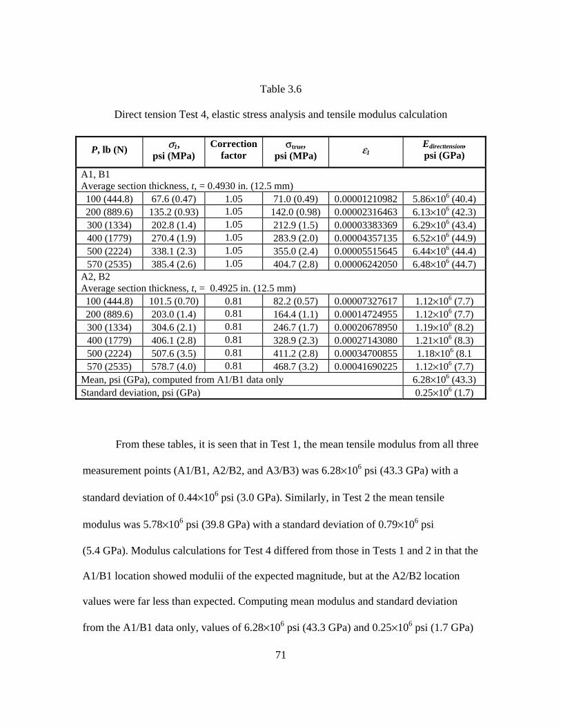
71
Table 3.6
Direct tension Test 4, elastic stress analysis and tensile modulus calculation
From these tables, it is seen that in Test 1, the mean tensile modulus from all three
measurement points (A1/B1, A2/B2, and A3/B3) was 6.28×10⁶ psi (43.3 GPa) with a
standard deviation of 0.44×10⁶ psi (3.0 GPa). Similarly, in Test 2 the mean tensile
modulus was 5.78×10⁶ psi (39.8 GPa) with a standard deviation of 0.79×10⁶ psi
(5.4 GPa). Modulus calculations for Test 4 differed from those in Tests 1 and 2 in that the
A1/B1 location showed modulii of the expected magnitude, but at the A2/B2 location
values were far less than expected. Computing mean modulus and standard deviation
from the A1/B1 data only, values of 6.28×10⁶ psi (43.3 GPa) and 0.25×10⁶ psi (1.7 GPa)
P, lb (N) σ1, psi (MPa)
Correction factor
σtrue, psi (MPa) ε1
Edirecttension, psi (GPa)
A1, B1 Average section thickness, t, = 0.4930 in. (12.5 mm) 100 (444.8) 67.6 (0.47) 1.05 71.0 (0.49) 0.00001210982 5.86×10⁶ (40.4) 200 (889.6) 135.2 (0.93) 1.05 142.0 (0.98) 0.00002316463 6.13×10⁶ (42.3) 300 (1334) 202.8 (1.4) 1.05 212.9 (1.5) 0.00003383369 6.29×10⁶ (43.4) 400 (1779) 270.4 (1.9) 1.05 283.9 (2.0) 0.00004357135 6.52×10⁶ (44.9) 500 (2224) 338.1 (2.3) 1.05 355.0 (2.4) 0.00005515645 6.44×10⁶ (44.4) 570 (2535) 385.4 (2.6) 1.05 404.7 (2.8) 0.00006242050 6.48×10⁶ (44.7)
A2, B2 Average section thickness, t, = 0.4925 in. (12.5 mm) 100 (444.8) 101.5 (0.70) 0.81 82.2 (0.57) 0.00007327617 1.12×10⁶ (7.7) 200 (889.6) 203.0 (1.4) 0.81 164.4 (1.1) 0.00014724955 1.12×10⁶ (7.7) 300 (1334) 304.6 (2.1) 0.81 246.7 (1.7) 0.00020678950 1.19×10⁶ (8.2) 400 (1779) 406.1 (2.8) 0.81 328.9 (2.3) 0.00027143080 1.21×10⁶ (8.3) 500 (2224) 507.6 (3.5) 0.81 411.2 (2.8) 0.00034700855 1.18×10⁶ (8.1 570 (2535) 578.7 (4.0) 0.81 468.7 (3.2) 0.00041690225 1.12×10⁶ (7.7)
Mean, psi (GPa), computed from A1/B1 data only 6.28×10⁶ (43.3) Standard deviation, psi (GPa) 0.25×10⁶ (1.7)

72
were obtained—favorably matching the Test 1 and Test 2 data. However, the average
modulus value at the A2/B2 location was 1.16×10⁶ psi (8.0 GPa), which is approximately
80 percent lower than all other computed values.
To explain the significantly lower modulus at the A2/B2 location in Test 4, the
load-strain history for this test was reviewed. Referencing Figures 3.13 and 3.14, it is
seen that Test 4 peaked at a maximum load value of approximately 625 lb (2,780 N),
which is nearly 50 percent lower than the maximum value in other tests. Coupling the
significantly lower failure load with the fact that a reasonable modulus was observed at
the A1/B1 location (indicating that the specimen material was not globally deficient in
some way) leads to the indication that damage was incurred in the specimen, at the
notched section, prior to beginning the test. This is further supported by comparison of
the tension test’s computed modulus value and the reduced modulus value computed
from the flexural test data—1.16×10⁶ psi (8.0 GPa) versus 0.79×10⁶ psi (5.4 GPa)—
which are in close agreement. From these observations, it is hypothesized that the
specimen in Test 4 was damaged during de-molding or handling prior to the test, and
microcracks were present in the notched area at test initiation. With application of load,
the microcracks immediately began to grow and coalesce, following the significantly
softer load-strain path seen for post-crack response in the flexure tests. Disregarding the
Test 4 A2/B2 data, the tensile modulus values computed from the direct tension tests are
in very close agreement with that computed from the flexural tests, as seen in Table 3.7.

73
Table 3.7
Tensile modulus comparison, tension tests and flexural tests
Test Mean modulus, psi (GPa)
Standard deviation, psi (GPa)
Tension Test 1 6.28×10⁶ (43.3) 0.44×10⁶ (3.0) Tension Test 2 5.78×10⁶ (39.8) 0.79×10⁶ (5.4) Tension Test 3 6.28×10⁶ (43.3) 0.25×10⁶ (1.7) Flexural tests 5.70×10⁶ (39.3) 1.1×10⁶ (7.6)
Mean 6.01×10⁶ (41.4) Standard deviation 0.31×10⁶ (2.1)
3.6 FE mesh refinement analysis
To ensure that the FE model results (at the points studied) were not subject to
mesh dependency, a mesh refinement analysis was performed. In the analysis, the FE
model used for the stress state study was meshed with a range of element sizes, varying
from approximately 0.25 in. (6.3 mm) by 0.25 in. (6.3 mm) by 0.25 in. (6.3 mm) to
0.05 in. (1.3 mm) by 0.05 in. (1.3 mm) by 0.05 in (1.3 mm). Computed stress-load
histories at the A1 and A2 locations were used as the basis for determining the influence
of mesh size on results. In Figure 3.32, the stress-load histories for the A1 location are
shown, and in Figure 3.33 the same histories are shown at a smaller scale to better
visualize the difference in results. From these plots, it is seen that at a load level of
approximately 1,000 lb (4,448 N), differences between stress levels are minimal, with
magnitudes less than 1 percent. Similar plots for the A2 location are given in Figures 3.34
and 3.35, and it is again seen that the difference between stress states as a result of mesh
refinement was minimal. From these data, it was concluded that with the 0.1-in.

74
(25.4-mm) mesh size used in the FE analysis, the model results were not subject to mesh
size dependency.
Figure 3.32 Mesh refinement analysis, A1 location.
Figure 3.33 Mesh refinement analysis, A1 location (smaller scale).

75
Figure 3.34 Mesh refinement analysis, A2 location.
Figure 3.35 Mesh refinement analysis, A2 location (smaller scale).

76
3.7 Post-crack tensile softening
In addition to studying initial linear-elastic response, the direct tension tests also
allowed for direct measurement of the fiber’s bridging capacity after crack formation in
the cementitous matrix. From the literature, the discontinuous fibers’ primary influence
occurs after failure of the cementitous matrix, when microcracks are growing and
coalescing into larger, widening macrocracks. This is a result of the fiber bridging and
failure mechanisms that take place during macrocrack formation and growth in the brittle,
cementitous material, which translates into a softening load-displacement curve after
reaching maximum load. It is expected that the benefit of these fibers in the VHSC
material would be even more pronounced than in conventional concrete due to the
increased brittleness that accompanies the elevated compressive strengths.
To study the specimens’ post-crack softening, data from the A2 and B2 gage
locations in Tests 1 and 2 are presented in Figure 3.36. Data from Test 4 are not
presented because of the apparent presence of damage prior to testing, and the resulting
unrepresentative response that occurred. In contrast to previous presentation of the direct
tension test data, the applied force is expressed in terms of internal stress at the notched
cross section instead of applied load. Note that the stress was computed as the nominal
cross-section stress (i.e. P/A), and the 0.81 correction factor calculated from Figure 3.31
was not used. This was done based on the assumption that once the section fully cracked,
stress concentration at the notch was generally relieved, and therefore the stress state
more closely approached the simple nominal condition. The crack opening width was
taken directly from the strain gage measurements, assuming once crack formation began

77
all of the strain in the notched area localized to the single macrocrack. Therefore, with a
strain gage length of 1 in. (25.4 mm), the crack opening was simply computed as the
strain measurement (in units of inch per inch) multiplied by the 1-in. (25.4-mm) gage
length.
Figure 3.36 Tension Tests 1 and 2: Stress-crack opening relationship.
Figure 3.36 shows general agreement between Tests 1 and 2 in terms of the nature
of the material’s post-crack tensile softening. In both tests the nominal stress peaked
between 1,000 psi (6.9 MPa) and 1,100 psi (7.6 MPa). After formation of the macrocrack,
the tests showed some difference in response, where the specimen in Test 1 immediately
exhibited strength decay while Test 2 maintained the peak load for a short time before
decaying. This is attributed to the stochastic nature of fiber distribution in the cementitous
matrix, where in Test 2 the fibers provided sufficient bridging at the crack to maintain the
peak load for a short time before complete failure.

78
Noting these differences provides support to conclusions drawn with regard to
ultimate failure variability observed in the flexure tests. The direct tension test results
showed that after reaching the matrix cracking strain, which coincided with the point of
peak stress in the specimen, the response may immediately transition to a strain softening
condition, or the stress level may be maintained as the crack initially opens and then
softening begins. It is hypothesized at this point, and will be studied in more detail with a
numerical model, that this variability in transition from brittle matrix failure to fiber-
controlled strain softening was a significant contributor to the wide range of ultimate
displacements observed in the flexural tests.
Regardless of response characteristics in the immediate vicinity of peak load,
once strength decay began, both tests exhibited similar trends. The strength loss after
peak was nonlinear, and appeared to asymptotically approach the zero stress level. The
data showed that although the decay was asymptotic in nature, once the crack opening
width reached approximately 0.025 in. (0.6 mm), or approximately 1/32 of an inch, the
specimens’ resistance to load was negligible. This is of significance because most work
in the literature reports that maximum crack opening width can generally be calculated as
a function of the fiber length—with a commonly accepted value of approximately
one-half of the fiber length (note that the majority of reported data is given with respect
to fiber types other than glass, with very little information available for fiberglass fibers).
Applying the literature-reported correlation between maximum crack width and fiber
length to the fiberglass-reinforced specimens, with 1-in. (25.4-mm) long fibers used in
production, it might be expected that the crack opening could grow to approximately

79
0.5 in. (12.7 mm) before losing all resistance to load. Although the tension tests were not
conducted until loads dropped to exactly zero, based on the nature of the recorded
response, it was not expected that a 20-fold increase in crack opening would occur before
complete failure took place.
Reviewing the stress versus crack opening relationships given in Figure 3.36, and
giving specific attention to the maximum stress levels reached by the specimens, it is
noted that the peak stress of approximately 1,050 psi (7.2 MPa) differs by approximately
45 percent from the mean cracking strength of 1,887 psi (13.0 MPa) computed in the
flexural experiments. Returning to the elastic FE analysis discussed in Section 3.5, it is
suggested that the seeming disparity between cracking strengths documented in the two
types of experiments is a result of stress concentrations developed at the notch tips in the
direct tension test specimens. To further explain, first recall that the stresses given in
Figure 3.36 were computed from the load, P, and gross cross-sectional area, A, at the
notch. Justification for this was based on the assumption that after initial yield occurred,
the specimen was fully cracked at the notch, and therefore the stress concentrations had
been relieved by formation of the crack. However, during that portion of the load history
leading up to the yield point, the section was not cracked, and therefore the stress
concentrations were present at the notch and were working to initiate a crack at that
location. Because of this, it is hypothesized that the peak stress at the notched section
should not be nominally calculated as P/A, as done in Figure 3.36. Rather, the peak
should be calculated based on the stress concentration that existed during final stages of
the linear-elastic response.

80
To support inclusion of the stress concentration effect in the data, Figure 3.37
shows a stress distribution calculated from the FE model at a load level of 1,100 lb
(4,893 N). From this, it is seen that the maximum stress at the notch tip was approxi-
mately 2,070 psi (14.3 MPa), as compared to the nominally calculated value of 1,050 psi
(7.2 MPa). This shows that, based on the notch geometry, stress concentration resulted in
peak stresses that were approximately twice the nominal. Assuming that the maximum
stress at the notch tip was the driving stress behind initiation of matrix cracking (which is
accepted based on experimental observations of crack propagation beginning at the notch
tips), then it is reasonable to conclude that the maximum stress at initiation of crack fail-
ure was approximately 2,070 psi (14.3 MPa). This maximum stress value differs by only
10 percent from that calculated in the flexure experiments, and consequently indicates
much greater agreement between the flexural and tensile experimental results.

81
Figure 3.37 FE stress distribution and concentration at tension test specimen notch.
In consideration of the foregoing peak stress analysis, and in further consideration
of the argument to use nominal stresses to describe the post-crack response, a recom-
mended internal stress versus crack opening curve was derived and is presented in Figure
3.38. Peak stress for the recommended curve was taken to be 2,070 psi (14.3 MPa),
which corresponds to the point at which brittle failure occurs within the cementitous
matrix. It is assumed that stress decay immediately after matrix cracking occurs rapidly,
with stress levels dropping to the nominally calculated values, at which point the fibers

82
are engaged to inhibit crack growth and ultimate failure. As the crack opening progres-
sively widens, the internal stress resistance drops in accordance with the trend measured
in the tension experiments, until stresses fall below 100 psi (0.7 MPa), or less than 5 per-
cent of the peak.
Figure 3.38 Recommended stress versus crack opening relationship for VHSC.
It is expected that this response curve can be used for input to material models
implemented in nonlinear analyses of the thin panel response, and will also be of use in
comparison to post-crack response predictions generated from micromechanical models
published in the literature. Note that once the fibers are fully engaged at a stress of
approximately 1,100 psi (7.6 MPa), the recommended response curve does not maintain
the material strength with small increases in crack opening, as seen in Test 2. Rather, to

83
provide a conservative estimate of post-crack response the recommended curve follows
the trend seen in Test 1, where the strength immediately decayed with increases in crack
width, providing a conservative lower bound on the material’s estimated post-crack
ductility.
As previously stated, post-crack response of the material is governed by the
bridging mechanism of the discontinuous fibers. It has been presented in the literature
that various failure modes may occur in the fibers—such as fiber pullout from the
cementitous matrix and fiber rupture if sufficient bond strength between the fiber and
matrix exists—and these failure modes have significant influence on the nature of the
post-crack response. This considered, after completion of the direct tension tests, the
specimens’ cracked sections were studied with an optical microscope to provide insight
into the types of failures that occurred. Since the specimens were not completely ruptured
in the experiments, it was possible to remove them from the test fixtures and observe the
fiber conditions at the crack as they existed at test completion. Images taken with the
optical microscope are shown in Figures 3.39 through 3.42.
As seen, two of the major fiber failure modes documented in the literature (fiber
rupture and fiber pullout) were present. Also seen were fiber bundles still bridging the
crack, which provided the small resistance to load remaining at test completion. Most
interestingly, a condition of fiber alignment with the crack direction was observed.
Considering that the fibers were randomly dispersed in the cementitous matrix, it should
be expected that some amount of the fibers would be oriented transverse to the direction
of load, and thus would be generally aligned with the crack direction. This is of particular

84
interest because all documented works reviewed for this project only considered fibers in
terms of their direct contribution to crack opening resistance, analogous in behavior to
small beams that bridged the crack in the cementitous material. However, in the case of
fibers aligned with the crack, it is possible that the fibers represented a weakened plane in
the matrix, allowing the crack to propagate more easily along the fiber/cementitous
matrix interface. From this observation and the postulate of its impact on response, more
in-depth research at the meso- and microscale levels might be conducted to understand
the impact of fiber-crack alignment on macroscopic response.
Figure 3.39 Tension test specimen, broken glass fibers.

85
Figure 3.40 Tension test specimen, bridging fibers at test completion.
Figure 3.41 Tension test specimen, mass of fibers—some broken and some aligned with crack.

86
Figure 3.42 Tension test specimen, fibers pulled from cementitous matrix.

87
CHAPTER IV
MICROMECHANICAL MODELS
In the preceding chapters, experimental data were presented which
(a) characterized flexural response of the 0.5-in.-thick (12.7-mm) panels and (b) directly
measured the post-crack tensile softening behavior of the discontinuously reinforced
material. Although these data provided a thorough description of the hardened material
response to flexural and tensile loads, they were also limited to a macroscopic under-
standing of material performance. Having noted the benefit of studying the material at
multiple length scales, it was also of great interest to consider the discrete interaction
between fibers and the cementitous matrix. In doing so, the fiber failure modes and
resulting impact on macroscopic ductility could be better understood, leading to future
intelligently engineered improvements in the discontinuous reinforcing scheme.
The above considered, included in the research project was an in-depth review of
a series of micromechanical models used to derive estimates of macroscopic ductility
from mesoscale descriptions of the fiber/matrix interaction. These models allowed for
consideration of various interface conditions and fiber failure modes, and when compared
to the direct tension test data they provided a greater understanding of the mesoscale
mechanics driving the macroscopic response.
In the literature, numerous works have been published which study the
micromechanical interaction between discontinuous reinforcing fibers and a cementitous

88
matrix. Significant contribution in this area has been made by V.C. Li and his associates,
with a series of papers published to present techniques for calculating the bridging stress
versus crack opening function of discontinuously reinforced concrete [21, 23, 24, 26,
29, 30]. The general approach taken in these studies is progressive in nature, considering:
• Response of a single embedded fiber under tensile load when oriented normal to
the crack plane.
• Response of a single embedded fiber when oriented at angle to the crack plane.
• Probabilistic effects of random fiber dispersion throughout a matrix and resulting
cumulative effects on the macroscopic tensile performance.
• Potential for fiber rupture and its effect on brittle failure of the material.
• More complex conditions such as slip-friction hardening or softening during fiber
pullout, and their influence on the material’s post-crack tensile softening.
Each of these aspects of micromechanical interaction between discrete fibers and
a surrounding matrix is discussed in detail in the following sections, along with
comparisons between analytical predictions and the experimental data.
4.1 Single fiber pullout model
To formulate the micromechanically based, analytical procedure for
determination of fiber reinforced concrete’s tensile response, Li et al. [23, 24, 26] first
adopt a foundational model to describe the basic fiber and concrete matrix interaction.
The model, shown in Figure 4.1, includes a single discontinuous fiber embedded in a
cementitous matrix, with the fiber oriented normal to the surface of the crack plane. In
the first formulation of this model, it is assumed that the fiber tensile strength is sufficient

89
to prevent rupture under tensile load, and therefore the failure mode is pullout from the
cementitous material. It is also assumed that the fiber has a finite embedment length,
Lembed, such that when it is loaded with an axial load, Pf, an interface stress, τif, is
developed, which is maximum at the crack face and decays over the finite length. As the
tensile load is increased, the interface stress will eventually reach the bond strength
between the fiber and the cementitous matrix, τifmax, and a slip-plane will begin to form
along the fiber length, beginning at the crack surface and progressing to the fiber end.
Once the maximum interface stress has progressed to the fiber tip, and the slip-plane
between fiber and matrix has been fully formed, the fiber will begin to pull out of the
matrix. The phase of fiber response up to the point of full slip-plane formation is referred
to as the debonding phase, and is generally characterized by a stiff, positive slope
response in a load versus crack opening plot.

90
(a) Initial interface stress distribution before reaching bond strength
(b) Progression of maximum interface stress along fiber length
(c) Interface stress at maximum load (end of debonding phase)
Figure 4.1 Single fiber pullout model at various load stages.
Before developing the mathematical expressions to describe the response of the
single fiber model, three additional assumptions are adopted regarding the nature of the
interface between the fiber and the concrete. These assumptions will be revised later in

91
the progressive model development; however, for the initial model formulation, the
following are held to be true:
• The fiber bond within the matrix is fully frictional.
• The interface bond strength, τifmax, is constant.
• During debonding, elastic stretch of the fiber gives rise to the crack opening.
Based on the fiber model shown in Figure 4.1 and the accompanying assumptions
given above, Li [24] presents the following equations to describe the load versus
displacement relationship for an axially loaded bridging fiber.
for δ ≤ δ0 (15)
(16)
where,
δ = crack opening that results from an applied tensile load
δ0 = crack opening at end of the debonding phase
Ef = fiber elastic modulus
df = fiber diameter
From equations 15 and 16, it is seen that in this analytical approach the
relationship between crack opening width and applied load during fiber debonding is a
function of the fiber physical properties (i.e. size—diameter and embedment length—and
tensile modulus) and the interface bond strength between the fiber and the cementitous
matrix. For the material considered in this study, the fiber physical properties can be
taken from the published data given in Table 2.1, with Ef equal to 11.4×10⁶ psi
2)( max
3 δτπδ ifff
f
dEP =
ff
ifembed
dEL max
2
0
2 τδ =
92
(78.6 GPa) and df equal to 0.0383 in. (0.97mm) (df calculated based on an area equivalent
to the total roving cross-sectional area). With fibers chopped to 1-in. (25.4 mm) lengths
in the production process, for simplicity Lembed can be taken equal to one-half of the fiber
length, or 0.5 in. (12.7 mm).
With the fiber physical properties as given above, τifmax, or the interface bond
strength between the fiber and the cementitous matrix, is left to be defined before the
crack opening versus applied load relationship can be determined. To determine the
fiber/matrix bond strength, a precise experimental procedure requiring special equipment
must be used, and as a result was beyond the scope of this study. In the micromechanical
model presentations by Li et al., comparisons to experimental data are given, along with
fiber material properties and bond strength data, but the body of this work was focused on
steel, polymer, and synthetic fibers, and no information on glass fibers was available.
Further review of the literature provided no additional information on glass fiber bond
strengths; therefore, published bond strengths for other fiber types were considered as a
means to identify a reasonable range of values that might be expected for the glass fiber
condition. From review of the literature, typical fiber bond strengths for various fiber
types in a cementitous matrix are given in Table 4.1.

93
Table 4.1
Published fiber/matrix bond strengths for various fiber types
Fiber type1 Fiber modulus, Ef, psi (GPa)
Bond strength, psi (MPa) Ref.
steel 29×106 (200) 870 (6) [25] steel 30.4×10⁶ (210) 609 (4.2) [26]
straight steel 30.4×10⁶ (210) 333-609 (2.3-4.2) [33] hooked steel 30.4×10⁶ (210) 507-653 (3.5-4.5) [33]
carbon fiber 5.5×10⁶ (38) 255-450 (1.76-3.10) [28] carbon fiber 25.4×10⁶ (175) 58 (0.4) [53]
polypropylene 1.7×10⁶ (11.9) 116 (0.8) [26] monofilament polypropylene 0.145×10⁶ (1) 14 (0.1) [33]
fibrillated polypropylene 0.145×10⁶ (1) 116 (0.8) [33]
polyvinyl alcohol (40 μm dia.) 3.2×10⁶ (21.8) 320/4540 (2.21/31.3)2 [36] polyvinyl alcohol (14 μm dia.) 8.7×10⁶ (60) 631/4873 (4.35/33.6)2 [36]
polyethylene 17.4×10⁶ (120) 145 (1.0) [25] polyethylene 17.4×10⁶ (120) 218 (1.5) [25] polyethylene 17×106 (117) 101/0 (0.7/0)1 [36] Spectra 900 17.4×10⁶ (120) 148 (1.02) [23]
Spectra 900 (individual fiber) 3 148 (1.02) [54] Spectra 900 (bundle of 20 fibers) 3 48 (0.328) [54] Spectra 900 (bundle of 40 fibers) 3 73 (0.502) [54] Spectra 900 (bundle of 57 fibers) 3 73 (0.505) [54]
Spectra 900 (bundle of 118 fibers) 3 51 (0.352) [54]
nylon 0.72×10⁶ (5) 23 (0.16) [21] nylon 3 7 (0.05) [33]
nylon (individual fiber) 3 23 (0.16) [54] nylon (bundle of 220 fibers) 3 7 (0.051) [54] Kevlar 49 (individual fibers) 3 653 (4.50) [54]
Kevlar 49 (bundle of 1000 fibers) 3 29 (0.198) [54] 1 as designated in the referenced work 2 frictional bond strength/chemical bond strength 3 no value provided
As seen in Table 4.1, a relatively large range of bond strength values have been
reported in the literature, varying from as low as 7 psi (0.05 MPa) for nylon fibers up to
approximately 4,900 psi (37.9 MPa) for polyvinyl alcohol (PVA) fibers. Noting that

94
significant variability is seen even between fibers of similar type (for example,
monofilament versus fibrillated polypropylene), from the data it is apparent that the
debonding mechanisms and associated fiber bond strength are not simply a function of
fiber type. Rather, it is more likely that the fiber/matrix bond relationship arises from a
large number of complex variables, all of which combine to influence the single bond
strength model parameter. The subject of fiber/matrix interface has been studied in detail
in an effort to fully understand the phenomena associated with failure of the fiber/matrix
interfacial transition zone, and Li and Stang [33] provide a listing of key works on the
topic [24, 26, 29, 55-58]. Li and Stang [33] also provide discussion of several significant
factors influencing the fiber/matrix interface bond, which include:
• Microstructure of cementitous matrix (particle density, microstructure strength,
microstructure stiffness, etc.) surrounding the fiber.
• Lateral confining stresses around the fiber (based on an assumption that the bond
interface strength is partly governed by a Coulomb-type friction law).
• Extent of cementitous material shrinkage during aging, resulting in reduction of
Coulomb friction effect.
• Fiber surface geometry, which enhances or degrades frictional bond.
• Fiber surface chemical attraction to cementitous matrix; documented for
hydrophilic and hydrophobic PVA fibers (their basic hydrophilic nature being
responsible for the extremely high chemical bond strengths given in Table 4.1).
• Fiber surface hardness – soft fibers (such as nylon or polypropylene) being
abraded during pullout which creates a slip-hardening effect; hard fibers (such as

95
steel) causing damage to the matrix and softening the fiber/matrix interface,
resulting in a slip-hardening effect during pullout.
• Fiber bundling, arising from poor dispersion of fibers in the matrix, results in a
change in apparent fiber surface available for bond to the matrix; glass fibers can
be prone to this effect [54].
Considering the numerous factors that affect the nature of the fiber/matrix bond
interaction, it is apparent that simple estimation of the relationship for glass fibers in the
densified, VHSC matrix is difficult at best. However, a potential range of glass fiber bond
strengths between 150 psi (1 MPa) and 600 psi (4.1 MPa) might be taken as an initial
estimate, disregarding the very low nylon strengths and the highly elevated PVA
strengths.
With the assumed range of debonding strengths, equations 15 and 16 were used to
calculate the crack opening displacement, δ, as a function of the applied fiber load. The
crack opening versus load curves for interface bond strengths of 150 psi (1MPa) and
600 psi (4.1 MPa) are given in Figure 4.2. As seen, the variation in bond strength results
in significant variability in the maximum load and crack opening width associated with
the debonding phase.

96
Figure 4.2 Single fiber axial load versus crack opening, debonding phase.
After developing an estimate of the single fiber response during the debonding
phase, it is necessary to consider the response during pullout from the matrix. To describe
fiber response during the pullout phase, Li [24] gives the relationship between an applied
end load and resulting fiber displacement to be,
for δ0 ≤ δ ≤ Lembed (17)
The results of equation 17, based on interfacial bond strengths of 150 psi (1 MPa)
and 600 psi (4.1 MPa), were combined with the debonding phase curves and are shown in
Figures 4.3 and 4.4. Figure 4.3 shows only a portion of the pullout curve so that the
model’s transition from the debonding phase to the pullout phase can be seen. Figure 4.4
shows the pullout phase curve over the full range of response.
)1()( 0max
embedfembediff L
dLPδδ
πτδ−
−=

97
Figure 4.3 Single fiber axial load versus crack opening, debond to pullout transition.
Figure 4.4 Single fiber axial load versus crack opening, complete pullout response.

98
From Figures 4.3 and 4.4, it is observed that equation 17 predicts a linear decay
in load resistance with pullout of the fiber, which is in keeping with the assumption of
constant frictional interface stress between the fiber and the matrix. Furthermore, it is
noted that the decay occurs over a pullout distance equal to the fiber embedment length,
or in this case, 0.5 in. (12.7 mm). Preliminary comparisons to the experimentally
observed crack opening response (reference Figure 3.38), indicate that some of the
simplifying assumptions adopted for the basic fiber pullout model may not be in
agreement with the mechanical response occurring in the glass fiber/VHSC composite.
4.2 Single fiber pullout model, inclination angle effects
After developing the single fiber model, assuming that the fiber is oriented normal
to the crack surface, Li [24] considers the influence of variable orientation with respect to
the crack surface—again through a single fiber model. To account for the effect of fiber
orientation angle with respect to the crack surface during both the debonding and pullout
phases, equations 15 and 17 are modified as shown in equation 18,
(18)
where,
φ = angle of orientation between the fiber’s axis and the crack plane, radians
f = snubbing coefficient, used to account for additional frictional resistance that occurs as a result of rubbing between the fiber and matrix at the crack face The orientation angle parameter, φ, is simply a function of the randomly
distributed fibers and covers a range of 0 radians to 1.5708 radians (0 to 90 degrees).
Similar to the frictional bond strength, the snubbing coefficient, f, is dependent on the
φδφδ fff ePP )(),( =

99
interface properties between the fibers and the matrix, and must be determined
experimentally. Because determination of the snubbing coefficient was also beyond the
scope of this study, reference was again made to the literature for coefficient estimates
associated with various fiber types. Snubbing coefficients found in the literature are given
in Table 4.2.
Table 4.2
Published snubbing coefficients for various fiber types
Fiber type Snubbing coefficient, f Ref. steel 0.8 [37]
carbon 0.5 [21] nylon 0.7 [25]
polypropylene 0.9 [25] polyethylene 0.8 [37]
polyvinyl alcohol 0.5 [27] Kevlar 49 0.6 [22]
Just as with the interfacial bond strengths, a large range of values is also found for
snubbing coefficients. Because the coefficients are not only a function of the fiber
properties, but also of the matrix in which the fibers are embedded, it is difficult to make
an exact estimate of an appropriate value for glass fibers. However, from Table 4.2 the
trend appears to be that higher coefficients are associated with more flexible fibers (such
as polypropylene and steel), while the brittle carbon fibers have the lowest value. This
might be expected because the snubbing coefficient is associated with friction as the
fibers are bent and rubbed over the matrix at the crack surface, and more flexible fibers
would be more easily bent. Because the glass fibers would be expected to behave in a
fairly brittle manner, their snubbing coefficient was estimated to be relatively low

100
(similar to the carbon fibers), with an assumed minimum value of 0.6. To provide for
consideration of a range of coefficient values, a maximum value of 0.8 was also
considered.
Before plotting the corrected debonding and pullout curves based on fiber
inclination angles, an additional assumption must be adopted. The assumption is
associated with the effect of bending failure in the fiber, and just as it was previously
assumed that the fiber would not rupture in tension, it is assumed that the fiber will not
break in bending. Note that Zhang and Li [53] indicate that this may not be a valid
assumption for brittle fibers such as glass and carbon, which will be further discussed
later in the analysis.
To examine the influence of fiber orientation angle on the fiber’s resistance to
load, an orientation angle of 0.524 radians (30 degrees) was assumed. The previously
calculated debonding phase curves for a normally oriented fiber are re-plotted in
Figures 4.5 and 4.6, augmented with curves based on the given orientation angle and
snubbing coefficients of 0.6 and 0.8. As seen, inclination of fibers to the crack plane can
have a significant effect on the debonding resistance. For both of the assumed bond
strengths, the combined effect of inclination angle and snubbing increased the maximum
debonding load by approximately 40 to 50 percent.

101
Figure 4.5 Single fiber axial load versus crack opening during debonding (fiber at angle to crack), τifmax = 150 psi (1 MPa).
Figure 4.6 Single fiber axial load versus crack opening during debonding (fiber at angle
to crack), τifmax = 600 psi (4.1 MPa).

102
. Considering equation 18, it is seen that the correction factor, efφ, for the single
fiber load versus displacement function is a constant for any given inclination angle and
snubbing coefficient. Therefore, since the nature of the debonding curve has been defined
in Figure 4.4, it is not necessary to repeat Figures 4.5 and 4.6 to show the pullout phase of
response. The pullout phase will simply be a linear decay of load as the crack opening
increases, with maximum crack opening width equal to the embedment length of 0.5 in.
(12.7 mm).
4.3 Composite material response model, pullout failure only
Having described the response of a single fiber when oriented normal and at angle
to the crack surface, it is necessary to consider the stochastic nature of fiber positioning
and orientation that arises from random distribution throughout the matrix. Li et al. [26]
address this by use of two probability density functions, which are given as:
(18)
(19)
where p(φ) describes the probability of fiber orientation angles for values of φ between 0
radians and 1.5708 radians (0 degrees and 90 degrees), and p(z) describes the probability
of embedment lengths, with z defined as the distance from centroid of the fiber to the
crack face.
Note that in the application of equations 18 and 19 Li et al. assume that the fibers
are uniformly dispersed throughout a three-dimensional cementitous matrix. Due to
geometry of the 0.5-in.-thick (12.7-mm) panels the assumption of three-dimensional
)sin()( φφ =p
fLzp 2)( =

103
uniformity may not be fully applicable in this case—with the fibers having greater
propensity for a two-dimensional, planar orientation. The probability density functions
given in equations 18 and 19 are used in this study for further development of the
composite bridging stress versus crack opening relationships, but future research might
consider the possible influence of a biased fiber directional orientation on results.
Utilizing the probability density functions given in equations 18 and 19, Li et al.
[26] develop an expression for bridging stress versus crack opening for a composite
cementitous matrix reinforced with randomly distributed fibers. The composite bridging
stress expression is
(20)
where,
σb(δ) = composite bridging stress as a function of the crack opening
Vf = the volume fraction of fibers in the composite material
Pf(δ,z,φ) is defined as the axially applied load for a single fiber as a function of
(a) crack opening, (b) fiber centroidal distance from the crack surface, and (c) fiber
orientation angle. Expressions are given for Pf(δ,z,φ) during the debonding (equation 21)
and pullout (equation 22) phases of response, and are as follows:
for δ ≤ δ1 (21)
for δ1 ≤ δ ≤ δ1 + Lembed (22)
φφφδπ
δσπφ
φ
φ
ddzzppzPd
VfL
z
zf
f
fb ∫ ∫
=
=
=
=
=2
0
cos)2(
02 )()(),,(
4)(
φδτηπφδ fifff edEzP ⎟
⎠⎞⎜
⎝⎛ += max
3)1(2
),,(
φδδπτφδ f
embedfembedif e
LdLzP ⎟⎟
⎠
⎞⎜⎜⎝
⎛ −−= 1
max 1),,(

104
where,
(23)
In equation 23, Vm and Em are the volume fraction and tensile modulus of the
cementitous matrix, respectively. In equations 21 and 22, δ1 represents the crack opening
width at which all fibers within the matrix have debonded, and only pullout resistance
remains—similar in concept to δ0 for the single fiber expressions. The expression given
for δ1 is,
(24)
Utilizing equations 21 and 22 in equation 20, Li et al. [26] derive closed-form
expressions for the composite crack bridging stress as a function of the normalized crack
opening width during the debonding and pullout phases of response. The final composite
crack bridging stress expressions are given in equations 25 and 26 below, with variable
definitions as given in equations 27 through 30.
for 0 ≤ δ2 ≤ δ2’ (25)
for δ2’≤ δ2 ≤ 1 (26)
(27)
ff
ifembed
dEL
)1(4 max
2
1 ητ
δ+
=
mm
ff
EVEV
=η
⎥⎥
⎦
⎤
⎢⎢
⎣
⎡
′−′=2
2
2
202 2)(
δ
δ
δ
δσδσ b
2
2202 )(1)( ⎥⎦⎤
⎢⎣⎡ ′−−= δδσδσ b
22
fLδδ =

105
(28)
(29)
(30)
Equation 25 describes the debonding phase of response, with δ2’ representing the
normalized crack opening width at which debonding is complete. Likewise, equation 26
describes the pullout response that follows the debonding phase. It is noted that in
presentation of these expressions, Li et al.[26] comment on their applicability to steel and
polymeric fibers, but no discussion is given to their validation for glass fiber applications.
Utilizing equations 25 and 26, composite bridging stress versus crack opening
functions were calculated based on the material parameters below, and are plotted in
Figures 4.7 (debonding phase only) and 4.8 (complete debonding and pullout response).
Note that although equations 25 and 26 are expressed in terms of the normalized crack
opening width, δ2, the plots are given in terms of the non-normalized value, δ. The
conversion from normalized to non-normalized values was done via simple application of
equation 27 to the x-axis component of the plots.
• Ef = 11.4×10⁶ psi (78.6 GPa)
• df = 0.0383 in. (0.97 mm)
• Vf = 0.03
• τifmax = 150 psi (1 MPa) and 600 psi (4.1 MPa)
⎟⎟⎠
⎞⎜⎜⎝
⎛
+=′
f
f
f
if
dL
E)1(2 max
2 ητ
δ
2
max
0f
ffif d
LVgτ
σ =
⎟⎟⎠
⎞⎜⎜⎝
⎛+
+= 2
2 14
2 f
ef
gπ

106
• Lf = 1 in. (25.4 mm)
• Vm = 0.97
• Em = 6.01×10⁶ psi (41.4 GPa)
• f = 0.6 and 0.8
Figure 4.7 Composite bridging stress as a function of crack opening, debonding phase.

107
Figure 4.8 Composite bridging stress as a function of crack opening, debonding and pullout phases.
Before continuing with further analysis, it is of importance to examine the
meaning of these post-crack bridging stress functions, and understand their relationship
to the material’s overall pre- and post-crack response. In the work presented by Li et al.,
discussion is not explicitly given to the specific relationship between the pre-cracked
stress state of the composite cross section and the post-crack tensile softening
contribution of the fibers—other than to clearly indicate that the given functions are only
derived for the post-cracked state. However, to use these functions to analyze the
experimental data, as well as to support the following finite element model development,
the relationship between pre- and post-crack conditions must be understood. Therefore,
the following arguments are postulated as a part of this study, and are subsequently
applied throughout the rest of this work.

108
Taken as presented in Figure 4.8, the bridging stress functions imply that at the
onset of cracking in the cementitous matrix, the bridging stress acting on the cracked
composite section increases from zero to some maximum value as the fibers go through
the debonding process. However, logically knowing that at the point of matrix failure
(which is assumed to be sudden based on a brittle failure mode) the stress in the
composite material is not zero, then the given stress versus crack opening function cannot
truly represent the material’s exact tensile softening performance. Rather, the distinction
is made here that these functions describe only the behavior of the bridging fibers during
the material’s post-crack response, which is preceded by the stress state dictated by the
uncracked matrix. For example, assume that for a given cementitous matrix, the
cracking stress corresponding to conclusion of linear-elastic response was approximately
100 psi (0.7 MPa). On rupture of the matrix, prior to which the cementitous material
carried all stress, the stress state must instantaneously be transferred to the bridging
fibers. If these fibers were characterized by the curves in Figures 4.7 and 4.8—with an
associated bond strength of 150 psi (1 MPa)—then (a) the fibers would be immediately
debonded, (b) a crack would open to approximately 0.0003 in. (0.008 mm), and (c) the
fiber pullout phase would immediately begin. On the other hand, if the fibers were
characterized by the 600 psi (4.1 MPa) bond strength curves, then the crack would
immediately open to approximately 0.00001 in. (0.00025 mm), and the debonding phase
would continue so that the section gained strength to approximately 400 psi (2.7 MPa).
From this interpretation of the bridging stress function’s meaning, the figures
show that at the onset of matrix cracking, the fibers have sufficient capacity to carry

109
approximately 100 psi to 400 psi of stress, depending on the magnitude of the interfacial
bond strength. Knowing from the experimental data that the matrix cracking strength for
the VHSC material is approximately 2,000 psi (13.8 MPa), debonding of the fibers would
be instantaneous, and the stress climb shown in Figure 4.7 would not even be observed.
Rather, the cross section would immediately transition to the fiber pullout phase of
response, progressing as shown in Figure 4.8. From this, revised bridging stress versus
crack opening functions that take into consideration the linear-elastic stress state present
in the matrix just prior to cracking are shown in Figure 4.9. The recommended bridging
stress versus crack opening function from the direct tension experiments (reference
Figure 3.38) is also shown.
Figure 4.9 Composite bridging stress as a function of crack opening, corrected for pre-crack linear-elastic response of the matrix.

110
As seen, the assumption of a significant drop in the tensile stress at the point of
matrix cracking generally matches the trend seen in the experimental data. However,
once the fibers are engaged in the pullout failure mode, the analytical model greatly over
predicts the residual ductility remaining in the specimen. This over prediction of ductility
during the pullout phase is further considered in the following variations of the model
formulation.
4.4 Composite material response model, fiber rupture effects
To further study the micromechanical model and its comparison to experimental
results, one of the fundamental assumptions previously made—namely that no fiber
rupture occurs—is revisited to determine its influence on response. At a minimum,
reconsideration of this failure mode is necessary because during post-experiment
examination of the direct tension specimens, ruptured fibers were observed (reference
Figures 3.39 and 3.41). Furthermore, it is qualitatively expected that the effect of fiber
rupture on the crack bridging stress function would be to cause a more rapid loss of
strength due to a reduction in the number of fibers available for bridging, which is the
nature of the difference between the calculated and experimental curves.
The observation of apparent fiber rupture in the post-experiment specimens is
validated by Maalej et al. [30], where they indicate that fiber rupture has been observed
in other studies of brittle fibers such as carbon and glass. In the same work, a methodol-
ogy is presented for incorporating potential fiber rupture into the micromechanical model
presented by Li et al. [26]. This fiber rupture and pullout model, as named in the cited

111
work, is implemented herein to gain quantitative understanding of the influence fiber
rupture may have on response.
Analogous to conventional reinforcing, the potential for fiber failure in the
composite material is a direct result of the interfacial bond strength, the embedment
length, the applied load, and the fibers’ tensile strength. Furthermore, it was previously
shown that the fiber’s orientation angle impacted the applied load required to achieve a
given crack opening width (reference Figures 4.5 and 4.6). Therefore, the fiber orienta-
tion angle is also included in the list of key parameters influencing the fiber rupture
potential.
The fiber rupture and pullout model is built around the concept of a fiber failure
envelope, which defines the combination of embedment lengths and orientation angles
that result in failure of a fiber with given tensile and interfacial bond strengths. As will be
seen, the failure envelope indicates that as the orientation angle between a fiber and the
crack surface increases, the embedment length required to develop a given fiber’s tensile
strength decreases due to the increased load felt by the fiber. Maalej et al. [30] give the
failure envelope equation as
(33)
where,
Lu(φ) = the embedment length at failure for a given orientation angle
Lc = the critical embedment length for a fiber oriented normal to the crack surface
Lc is further defined as,
(34)
φφ fcu eLL −=)(
max4 if
ffuc
dL
τσ
=

112
where,
σfu = the ultimate tensile strength of the fiber
Utilizing equations 33 and 34 with the following material parameters:
• σfu = 270,000 psi (1.9 GPa)
• df = 0.0383 in. (0.97 mm)
• τifmax = 600 psi (4.1 MPa)
• f = 0.6
the failure envelope can be plotted as shown in Figure 4.10. Review of the failure enve-
lope indicates that based on the assumed bond and tensile strengths, when fibers are ori-
ented normal to the crack plane (φ = 0 radians), an embedment length of approximately
4.25 in. (108 mm) is required for their full development. Likewise, the failure envelope
shows that the minimum embedment length required to rupture fibers, coinciding with
the maximum orientation angle (φ = 1.5708 radians), is approximately 1.75 in. (44 mm).

113
Figure 4.10 Fiber rupture failure envelope, τifmax = 600 psi (4.1 MPa).
Recognizing that the minimum fiber length required to achieve a given embed-
ment is two times Lembed, the failure envelope indicates that all fibers longer than 8.5 in.
(216 mm) will rupture, and all fibers shorter than 3.5 in. (89 mm) will only experience
pullout. Fiber lengths in-between will either rupture or pullout, depending on their angle
of orientation.
With a maximum fiber length of 1 in. (25.4 mm) used in the VHSC composite,
the rupture envelope implies that the fibers are not long enough to develop sufficient ten-
sile load to cause rupture, and therefore all fibers should pull out of the matrix during a
tensile failure of the composite. However, this is not in agreement with the experimen-
tally observed fiber rupture in the specimen, nor with conclusions drawn from the pullout
micromechanical model presented in Section 4.3.

114
Reviewing the expressions used to plot the failure envelope, it is seen in equa-
tion 34 that the variable defined with the least amount of accuracy is the interface bond
strength, or τifmax. The other variables either pertain to the fibers’ mechanical properties
(df and σfu), which are taken from the manufacturer’s published data, or are not deemed
to have as significant an impact (f). Using equations 33 and 34 again with the same
parameters, and assuming an orientation angle of 1.5708 radians (90 degrees), it can be
seen that the minimum bond strength required to cause rupture in 1-in.-long (25-mm)
fibers (with an embedment length of one-half of Lf) is approximately 2,100 psi
(10.3 MPa). Similarly, the bond strength required to cause rupture of all 1-in. (25-mm)
fibers with an embedment length equal to one-half of Lf is 5,000 psi (34.5 MPa). These
failure envelopes are shown in Figure 4.11. From this failure envelope analysis, it is indi-
cated that if fiber rupture occurred as a major failure mode in the composite material,
then the interfacial bond strength between the fibers and the high-strength cementitous
matrix may be much higher than initially estimated. From Table 4.1, for significant fiber
rupture to occur the glass fiber/matrix interface bond strength may be closer to the
chemical bond associated with PVA fibers rather than the frictional bond associated with
steel or others.

115
Figure 4.11 Fiber rupture failure envelope, τifmax = 2,100 (14.5 MPa) and 5,000 psi (34.5 MPa).
To account for the effects of fiber rupture on the composite response, Maalej et al.
[30] developed modified bridging stress expressions based on two distinct phases. The
first phase of response, termed the rupture phase, begins with the onset of fiber straining
and is concluded when all fibers with sufficient embedment length have ruptured. In
terms of the fiber rupture envelope, this means that all fibers with embedment length and
orientation angle plotting above the failure surface have experienced failure, and only
those fibers plotting below the surface remain intact. The second phase of response,
termed the pullout phase, constitutes that portion of the tensile response when the
remaining intact fibers pullout from the matrix as the crack bridging strength decays
to zero.

116
Assuming that the discontinuous fiber length falls within the failure envelope
limits (i.e., for τifmax = 5,000 psi (34.5 MPa) the envelope limits are 0.15 in. × 2 = 0.3 in.
(7.6 mm) and 0.52 in. × 2 = 1.04 in. (26.4 mm)), Maalej et al. [26] provide the following
expression to describe the initial portion of the rupture response phase,
for δ2 ≤ δc’’ (35)
where,
(36)
(37)
(38)
In equations 35 through 38, δ2, δ2’, σ0, f, Lf, df, η, Ef, and τifmax are as defined for
the pullout model in equations 27 through 30, and σfu is as given in equation 34.
Comparing equation 35 to equation 25, it is seen that they are of the same form, simply
with different definitions of applicability limits. This indicates that initial response of the
rupture and pullout model is similar to that of the pullout only model, characterized by a
fiber debonding phase even before fiber rupture begins. This debonding portion of
response can be thought of as the pre-peak portion of the rupture response phase, during
which the fibers are being loaded and the fiber stresses climb in preparation for either
rupture or pullout failure.
⎟⎟⎟
⎠
⎞
⎜⎜⎜
⎝
⎛
′−′=2
2
2
202 2)(
δ
δ
δ
δσδσ b
πδδ fcc e −′=″
f
cc L5.0
δδ =′
max
2
)1(4 if
ffuc Ef
dτη
σδ
+=
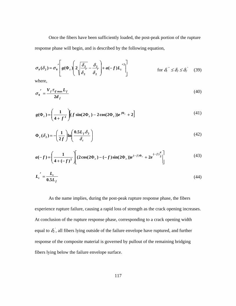
117
Once the fibers have been sufficiently loaded, the post-peak portion of the rupture
response phase will begin, and is described by the following equation,
for δc’’ ≤ δ2 ≤ δ2
’ (39)
where,
(40)
(41)
(42)
(43)
(44)
As the name implies, during the post-peak rupture response phase, the fibers
experience rupture failure, causing a rapid loss of strength as the crack opening increases.
At conclusion of the rupture response phase, corresponding to a crack opening width
equal to δ2’, all fibers lying outside of the failure envelope have ruptured, and further
response of the composite material is governed by pullout of the remaining bridging
fibers lying below the failure envelope surface.
⎥⎥
⎦
⎤
⎢⎢
⎣
⎡′−+
⎟⎟⎟
⎠
⎞
⎜⎜⎜
⎝
⎛
′−′Φ′=2
2
2
2
202 )(2)()( ccb Lfag
δ
δ
δ
δσδσ
f
fiff
dLV
2max
0
τσ =′
[ ]2))2cos(2)2sin((4
1)( 2 +Φ−Φ⎟⎟⎠
⎞⎜⎜⎝
⎛
+=Φ Φ cf
ccc eff
g
⎥⎥⎦
⎤
⎢⎢⎣
⎡+Φ−−Φ⎟⎟
⎠
⎞⎜⎜⎝
⎛
−+=−
−Φ− 2)()(
2 2))2sin()()2cos(2()(4
1)(πff
cc eeff
fa c
f
cc L
LL
5.0=′
⎟⎟⎠
⎞⎜⎜⎝
⎛⎟⎟⎠
⎞⎜⎜⎝
⎛−=Φ
c
fc
Lf δ
δδ 2
2
5.0ln
21)(
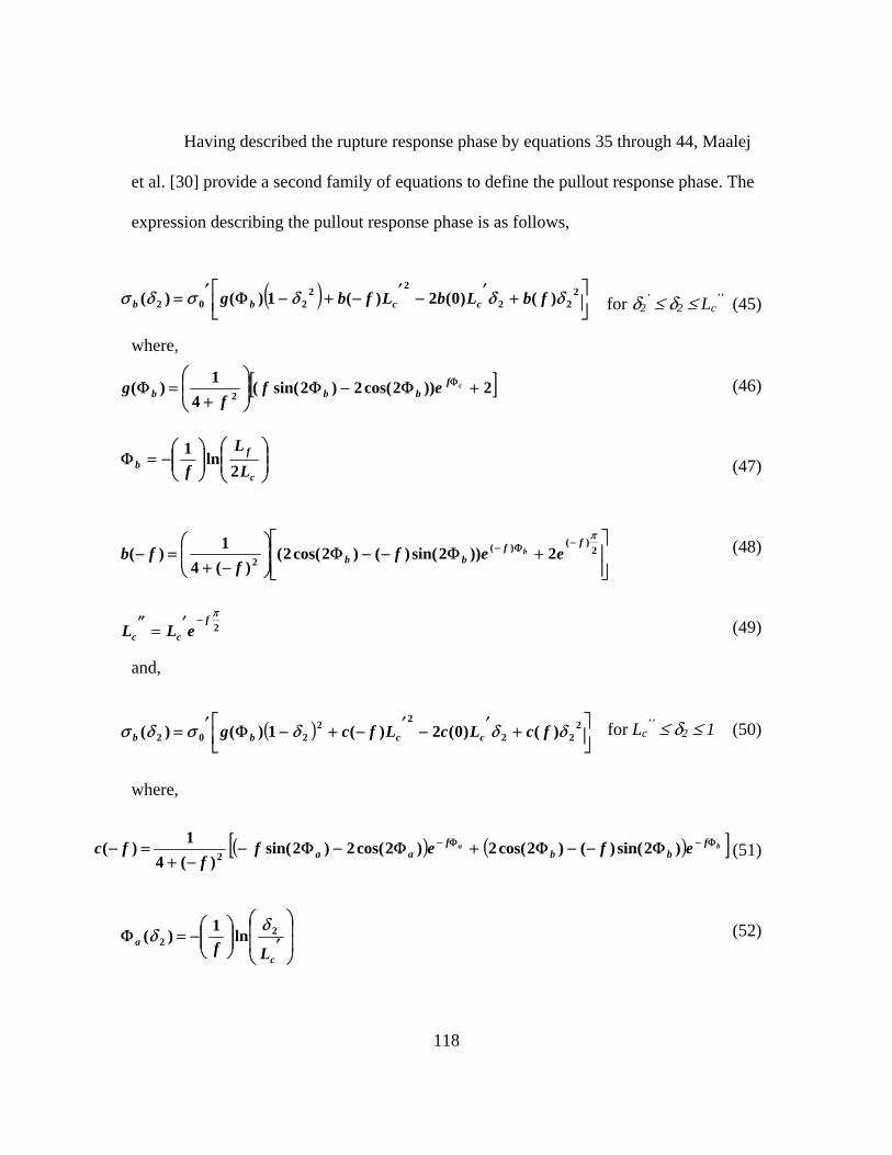
118
Having described the rupture response phase by equations 35 through 44, Maalej
et al. [30] provide a second family of equations to define the pullout response phase. The
expression describing the pullout response phase is as follows,
for δ2’ ≤ δ2 ≤ Lc
’’ (45)
where,
(46)
(47)
(48)
(49)
and,
for Lc
’’ ≤ δ2 ≤ 1 (50)
where,
(51)
(52)
( ) ⎥⎦⎤
⎢⎣⎡ +′−′−+−Φ′= 2
22
22202 )()0(2)(1)()( δδδσδσ fbLbLfbg ccbb
[ ]2))2cos(2)2sin((4
1)( 2 +Φ−Φ⎟⎟⎠
⎞⎜⎜⎝
⎛
+=Φ Φ cf
bbb eff
g
⎟⎟⎠
⎞⎜⎜⎝
⎛⎟⎟⎠
⎞⎜⎜⎝
⎛−=Φ
c
fb L
Lf 2
ln1
⎥⎥⎦
⎤
⎢⎢⎣
⎡+Φ−−Φ⎟⎟
⎠
⎞⎜⎜⎝
⎛
−+=−
−Φ− 2)()(
2 2))2sin()()2cos(2()(4
1)(πff
bb eeff
fb b
2πf
cc eLL−′=″
( ) ⎥⎦⎤
⎢⎣⎡ +′−′−+−Φ′= 2
22
22202 )()0(2)(1)()( δδδσδσ fcLcLfcg ccbb
( ) ( )[ ]ba fbb
faa efef
ffc Φ−Φ− Φ−−Φ+Φ−Φ−
−+=− )2sin()()2cos(2)2cos(2)2sin(
)(41)( 2
⎟⎟
⎠
⎞
⎜⎜
⎝
⎛
′⎟⎟⎠
⎞⎜⎜⎝
⎛−=Φ
c
aLf
22 ln1)(
δδ

119
Utilizing equations 35 through 52 to study the influence of fiber rupture on the
bridging stress functions, responses were calculated for interfacial bond strengths of
2,500 psi (10.3 MPa) and 5,000 psi (34.5 MPa). These response curves are shown in
Figure 4.12, uncorrected for the pre-crack stress state of the matrix.
Figure 4.12 Composite bridging stress functions from rupture and pullout model (uncorrected for pre-crack stress state).
From the rupture and pullout curves given above, the most noticeable observation
is that the peak bridging stress capacity of the fibers is drastically greater than that
calculated for the pullout only model (compare to Figure 4.9). However, on review of
equation 39 this is as should be expected, considering that the bridging stress capacity is
expressed as a direct function of the interfacial bond strengths, which are over an order of
magnitude higher than those assumed in the pullout only model. It is also observed that

120
for the 5,000 psi (34.4 MPa) bond strength condition, the composite response first
exhibits a sharp drop in capacity before transition to a more gradual loss of strength. The
sharp strength loss is a result of the fiber rupture mechanism in the model, described by
equation 39. In contrast, the 2,500 psi (17.2 MPa) bond strength curve does not show the
same sharp drop in capacity. This should also be expected based on the fiber rupture
envelope for the assumed bond strength, which indicates that 0.8 in. (20 mm) is the
shortest possible fiber length that could have sufficient embedment to instigate rupture
(i.e., fiber rupture will not occur for fibers with embedment less than 0.4 in. (10 mm)).
With fibers in the composite having a length of 1 in. (25 mm) (maximum embedment of
0.5 in. (12.5 mm)), only a small portion could develop sufficient tensile stress to fail in
rupture, and all others would pullout of the matrix—following the trend of the pullout
only model.
Just as with the pullout only model, the rupture and pullout model results must be
adjusted for the pre-crack stress state. Because the 5,000 psi (34.4 MPa) bond strength
curve indicates that the fibers have a maximum bridging capacity of approximately
2,200 psi (15.2 MPa), on failure of the matrix at 2,000 psi (13.8 MPa) the fibers should
be able to carry the stress without immediate strength loss. In fact, they would continue to
move through the debonding phase until a maximum stress of 2,200 psi was reached, and
then the rupture and pullout phase would occur. On the other hand, the 2,500 psi
(17.2 MPa) bond strength curve, which has a fiber bridging capacity of approximately
1,500 psi (10.3 MPa), would immediately transition to the pullout phase of response,
exhibiting an instant drop in strength of approximately 500 psi (3.4 MPa).
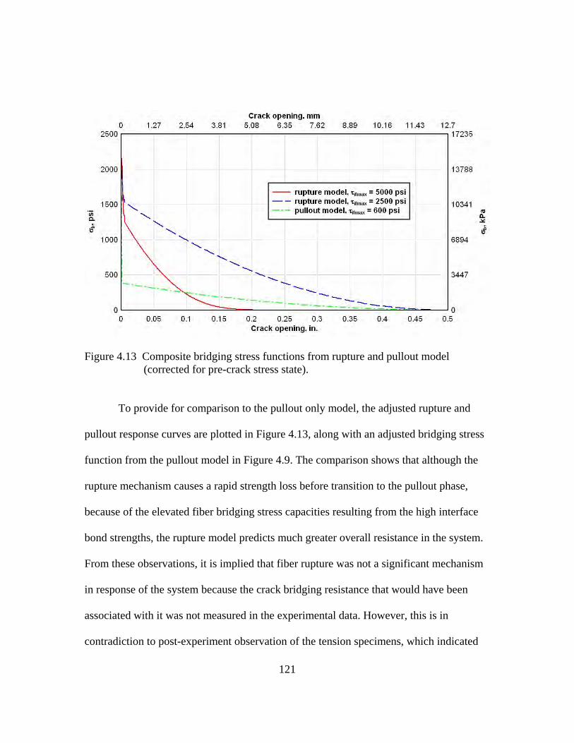
121
Figure 4.13 Composite bridging stress functions from rupture and pullout model (corrected for pre-crack stress state).
To provide for comparison to the pullout only model, the adjusted rupture and
pullout response curves are plotted in Figure 4.13, along with an adjusted bridging stress
function from the pullout model in Figure 4.9. The comparison shows that although the
rupture mechanism causes a rapid strength loss before transition to the pullout phase,
because of the elevated fiber bridging stress capacities resulting from the high interface
bond strengths, the rupture model predicts much greater overall resistance in the system.
From these observations, it is implied that fiber rupture was not a significant mechanism
in response of the system because the crack bridging resistance that would have been
associated with it was not measured in the experimental data. However, this is in
contradiction to post-experiment observation of the tension specimens, which indicated

122
that fiber rupture occurred. As an explanation for this discrepancy, reference is made to
documentation in the literature for bending failure modes in brittle fibers. Zhang and Li
[53] indicate that when exposed to bending stresses, brittle fibers, such as glass, can
experience rupture failure at loads much less than would be required for failure in pure
tension. Recognizing that because of the random fiber distribution in the matrix a certain
amount of fibers would have been exposed to a bending stress state, this could certainly
explain the observation of fiber rupture failure without the accompanying bridging
resistance.
4.5 Composite material response model, slip softening effects
The final failure mechanism considered in the micromechanical study is
associated with changes in the interfacial bond strength,τifmax, during the pullout phase.
Recall that in the initial formulation of the pullout only model, the assumption was made
that interfacial bond strength was constant throughout the crack opening event. However,
Li and Stang [33] have indicated that interfacial bond strength may not be constant with
fiber displacement, depending on the specific fiber and matrix properties. For soft fibers,
such as polypropylene, during fiber pullout the surrounding matrix may abrade the fibers
as the particles cut into the fiber surface. This tends to increase the fiber’s resistance to
pullout via an interlocking mechanism, and subsequently results in an increase in the
effective interfacial bond strength as pullout progresses (referred to as slip-hardening).
On the other hand, hard fibers such as glass or steel are indicated to potentially damage
the matrix along the interface in a manner so as to smooth the interfacial surface. This

123
results in a potential decrease in the interfacial bond strength during the pullout process,
which is documented in the literature as a slip-softening effect.
To account for the potential of slip-hardening or slip-softening effects, Li et al.
[26] present a simple polynomial expression for the interfacial bond strength as a
function of the crack opening width. The variable bond strength expression, given in
equations 53 and 54, is a function of two empirical parameters, a1 and a2. For crack
opening widths less than δ2’ (which corresponds to conclusion of the fiber debonding
phase), the interfacial bond strength equals the constant, τifmax, which should be expected
because slippage has not occurred. However, for displacements greater than δ2’, during
which time fiber pullout is occurring, the interfacial bond strength varies in the manner
defined for τ(δ2).
for δ2 ≤ δ2’ (53)
for δ2’ ≤ δ2≤ 1 (54)
Although the above expression is given to describe the slip softening bond
strength, Li et al. [26] do not provide values for a1 and a2 in association with glass fibers.
Since data are not available for direct use in equation 54, the softening function could be
bounded by two assumed bond strength decay curves, such that an estimate of the range
of slip softening effects could be made. To this end, a simple, linear bond strength decay
function is first given in equation 55.
max2 )( ifτδτ =
221max2 )( δδτδτ aaif −+=

124
for δ2
’ ≤ δ2≤ 1 (55)
where,
(56)
Given in equation 57, an exponential decay function was also developed to
consider a sharp loss of strength initially, which then becomes more gradual as the crack
opening increases.
for δ2
’ ≤ δ2≤ 1 (57)
It is notable that the idea of a sharp, exponential decay trend matches the nature of
the experimentally determined strength decay function. Further, the notion of a sharp
exponential bond strength decay is supported in commentary by Zhang and Li [53],
suggesting that the interfacial bond strength of glass fibers in a cementitous matrix is
derived more from chemical bonds rather than mechanical. If the bond is chemical in
nature, then it should be expected that during the fiber debonding phase, the maximum
bond stress would be reached with little displacement in the fiber, but after failure along
the interface, little residual strength would remain. The linear and exponential bond
strength decay functions from equations 55 and 57 are plotted in Figure 4.14. For these
curves, τifmax is assumed to be 600 psi (34.5 MPa), and a3 is -602.
max2232 )( ifa τδδδτ +⎟⎠⎞⎜
⎝⎛ ′−=
′−
−=
2
max3
1 δ
τ ifa
⎟⎟
⎠
⎞
⎜⎜
⎝
⎛=
−′+−
1
1)1(
max2
422
)(e
eif
δδ
τδτ

125
Figure 4.14 Linear and exponential fiber bond strength decay functions.
Finally, to determine the influence of a slip-softening effect on the composite
material response, the bond strength expressions can be incorporated into the bridging
stress equations given in Section 4.3 (pullout failure) and Section 4.4 (rupture failure).
Using the linear and exponential decay functions determined above, slip-softening curves
were calculated for the pullout model in Figure 4.15 and for the rupture and pullout
model in Figure 4.16. For comparison, each plot also contains the associated models’
constant bond strength functions, as well as the experimental data.

126
Figure 4.15 Composite bridging stress functions with linear and exponential bond strength decay (pullout model).
Figure 4.16 Composite bridging stress functions with linear and exponential bond
strength decay (rupture and pullout model).

127
Figures 4.15 and 4.16 show that the slip-softening effect can have significant
influence on the composite material’s tensile softening response. In both cases, the
assumption of linear bond strength decay resulted in a moderate change from the constant
bond stress condition, but the exponential decay condition showed a significant change in
the bridging strength function. Although the assumption of exponential bond strength
decay significantly reduced the rupture and pullout model’s bridging resistance during
the pullout phase, the model still estimates a bridging resistance that greatly exceeds that
measured in the laboratory. However, incorporating the slip-softening effect (exponential
strength decay) into the pullout model yielded a bridging function that more closely
approximated the experimental.
4.6 Summary of micromechanical model results
Although flexural and direct tension experiments conducted within the research
program provided thorough descriptions of the VHSC material’s response to load, the
data were limited to a macroscopic understanding of material performance. An in-depth
understanding of the mesoscale mechanics driving the global specimen response could
not be obtained, and therefore, a series of micromechanical models was used to study the
significance of interaction between fibers and the cementitous matrix.
Following the extensive research of V.C. Li and others, a set of progressive
micromechanical models were implemented, building from basic consideration of a
single fiber to inclusion of complicating factors such as stochastic fiber distribution and
slip-softening effects. Five distinct model formulations were studied, and included:
• Response of a single embedded fiber under direct tensile load.

128
• The influence of fiber inclination angle on pullout resistance and associated
maximum load.
• Use of probability density functions to apply the single fiber micromechanical
model to randomly reinforced materials.
• The potential for fiber rupture, and its influence on the composite bridging stress
function.
• Slip-softening and slip-hardening effects during fiber pullout, and their influence
on the composite bridging function.
Comparison of results to the direct tension test data indicated that the various
model formulations approximated certain aspects of the observed macroscopic response,
but they did not fully capture the VHSC’s tensile softening characteristics. However,
sufficient similarities between the predicted and measured responses were observed to
loosely support conclusions regarding key phenomena occurring at the mesoscale level,
providing groundwork for future study on the topic. For use in further discussion, the
recommended bridging stress function determined from the direct tension tests
(Figure 3.38) is repeated in Figure 4.17, with key portions of the curve marked for
reference.

129
Figure 4.17 Recommended bridging function from direct tension experiments.
Based on cumulative results from the micromechanical study, three distinct
components of the measured fiber bridging function can be considered. First, an initial,
sharp drop in strength was observed, denoted as portion A of the curve in Figure 4.17.
The micromechanical analysis indicated that this sharp drop in strength was as a result of
brittle cracking of the cementitous matrix and transfer of the tensile load to the bridging
fibers. On review of the results this should be expected, considering that at conclusion of
linear-elastic response in the cementitous matrix the material would fail in a brittle
manner, causing a rapid loss of strength until the reinforcement was engaged.
Interestingly, the models also showed that with proper engineering of the fiber

130
reinforcement, bridging strength enhancement could be observed, resulting in an overall
strengthening of the composite material.
At a tensile stress of approximately 1,100 psi (7.6 MPa), corresponding to point B
in the figure, the fibers were engaged to carry the tensile load and arrested the rapid
strength loss occurring in the matrix. Governed by physical fiber characteristics such as
length and diameter, as well as interfacial characteristics such as bond strength and
snubbing coefficient, the micromechanical models showed that with an assumed
interfacial bond strength of approximately 1,400 psi (9.6 MPa) the maximum fiber
bridging strength would be approximately 1,100 psi (7.6 MPa)—as observed.
The final component of the tensile response, denoted as portion C of the
recommended curve, was initially assumed to be associated with pullout of the fibers
after their engagement at point B. However, analyses indicated that if the post-crack
ductility were governed by frictional fiber pullout, then the expected bridging resistance
would be much greater than that observed—continuing to a maximum crack opening
width of approximately 0.5 in. (12.7 mm). However, the experimental data indicated that
full strength loss occurred at a maximum crack width of approximately 0.025 in.
(0.64 mm), much smaller than the model predicted value. Discounting the possibility of
frictional fiber pullout based on this observation, the potential for fiber rupture was
considered. Shown in Figure 4.12, it was seen that fiber rupture would cause a more rapid
loss of strength as compared to the pullout failure mode. However, rupture of the fibers
would have also coincided with a much greater fiber bridging strength—which is in
conflict with the experimental observations. Therefore, fiber rupture was also discounted

131
as the mechanism governing portion C of the tensile softening response. Finally, slip-
softening effects were studied to determine the potential for their influence on the ductile
portion of composite response. Figure 4.14 showed that with the assumption of a very
strong exponential decay function, calculated loss in the fiber bridging strength
approximated that seen in the experimental data. However, noting that the assumed
exponential decay function was based on an exponential raised to the fourth power
(reference equation 57), the implication was that very little bridging capacity existed after
fiber debonding—indicating that the assumption of frictional pullout resistance may not
be valid. Rather, it may be more likely that the bond between fibers and the cementitous
matrix was chemically based, such that after fiber debonding very little resistance to fiber
pullout could be achieved. This postulate of chemically based interface bonding is
supportive of all aspects of the measured fiber bridging function, and warrants further
investigation in future studies.

132
CHAPTER V
FLEXURAL FINITE ELEMENT MODEL
Having experimentally measured the panels’ response to flexural and tensile
loads, as well as having studied the mesoscale interaction between fibers and the
cementitous matrix, investigation of the VHSC panels was concluded with development
of two numerical models to calculate panel flexural response. The finite element models
were built using ABAQUS/CAE, Version 6.5-4, and simulated the third-point bending
experiments presented in Chapter II. Two approaches were taken in the model
development, and included the use of:
• Shell elements with a simple elastic-plastic material model.
• Shell elements with a concrete damage model and a user-defined post-crack
tensile softening function.
Initially, the FE model was formulated with a very simple elastic-plastic model,
with inclusion of strain hardening effects. This was used as a simple method to replicate
panel response based on the mean characteristics given in Table 2.3, and was compared
to the mean response function given in Figure 2.18. However, since the elastic-plastic
model was described solely from estimates of the pre- and post-crack material modulus,
without consideration of the true failure mechanisms occurring in the concrete, a more
fundamental concrete damage model was also used. The concrete model was primarily

133
chosen because of its capability to define different yield points in tension and
compression, along with its capability to define a post-crack bridging stress versus crack
opening function. Defining the bridging stress function from results of the direct tension
experiments and micromechanical analyses, the concrete model was expected to capture
the panels’ ultimate failure as well as their pre- and post-crack stiffness based on
fundamental characteristics determined in preceding portions of the project.
5.1 Shell element model with elastic-plastic material model
In the shell element model, the 10-in. (25.4-cm) by 40-in. (101.6-cm) flexural test
specimen was discretized with approximately 0.5-in. (12.7-mm) by 0.5-in. (12.7-mm)
shells, resulting in 1,620 total elements in the model. Four noded, linear shells were used
(ABAQUS element type S4R), with six degrees of freedom per node. With the given
discretization, 1,722 nodes were contained in the model, resulting in 10,332 degrees of
freedom (before application of boundary conditions). Note that eight noded, quadratic
shells (ABAQUS element type S8R) were also used initially, but did not show a
difference in results from the linear elements. Because of the increased computational
cost associated with the quadratic elements, the linear elements were used for the
remainder of the calculations.
Pin-roller boundary conditions were applied to the model in accordance with the
experimental setup. At one end of the model, 2 in. (50.8 mm) from the edge, a line of
nodes was restrained from translation in all three directions (pinned connection). At the
opposite end, also 2 in. (50.8 mm) from the edge, another line of nodes was restrained
only in two directions, free to translate in the direction of the panel span (roller
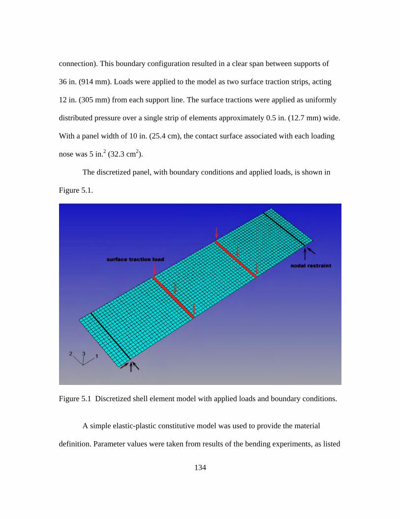
134
connection). This boundary configuration resulted in a clear span between supports of
36 in. (914 mm). Loads were applied to the model as two surface traction strips, acting
12 in. (305 mm) from each support line. The surface tractions were applied as uniformly
distributed pressure over a single strip of elements approximately 0.5 in. (12.7 mm) wide.
With a panel width of 10 in. (25.4 cm), the contact surface associated with each loading
nose was 5 in.2 (32.3 cm2).
The discretized panel, with boundary conditions and applied loads, is shown in
Figure 5.1.
Figure 5.1 Discretized shell element model with applied loads and boundary conditions.
A simple elastic-plastic constitutive model was used to provide the material
definition. Parameter values were taken from results of the bending experiments, as listed

135
in Table 2.3. Accordingly, Young’s modulus, Poisson’s ratio [52], first-crack strength,
and the post-crack plastic hardening were taken to be 5.7×10⁶ psi (39.3 GPa), 0.23,
1,887 psi (13 MPa), and 0.79×10⁶ psi (5.4 GPa), respectively. The resulting stress-strain
curve is given in Figure 5.2.
Figure 5.2 Elastic-plastic stress versus strain curve.
Because significant softening of the system stiffness matrix was expected during
the post-crack response, the Riks method—a variant of the arc length method—was used
to conduct the analysis. The benefit of the Riks analysis method is that instead of using a
tangent stiffness approach to calculate transitions in the system stiffness, it uses a
swinging arc method to determine increments of load (either increasing or decreasing),
which can subsequently capture global system softening. The Riks analysis parameters

136
were set such that the arc length was automatically incremented based on changes in the
system stiffness, with stopping criteria set for either attainment of a maximum specified
load or a maximum displacement of 0.75 in. (19 mm) at the specimen third-point.
The thickness of all shell elements was set to 0.467 in. (11.9 mm) as given in
Table 2.3, yielding an element aspect ratio of approximately 1 in all dimensions.
Simpson’s integration rule was used for integration points through the element thickness,
and the number of integration points was varied to evaluate the effect on results.
With the model constructed as described, load versus third-point displacement
curves were calculated for 3, 5, 7, and 19 integration points through the element
thickness. Results, along with the mean response curve and response envelope from
Figure 2.18, are given in Figure 5.3.
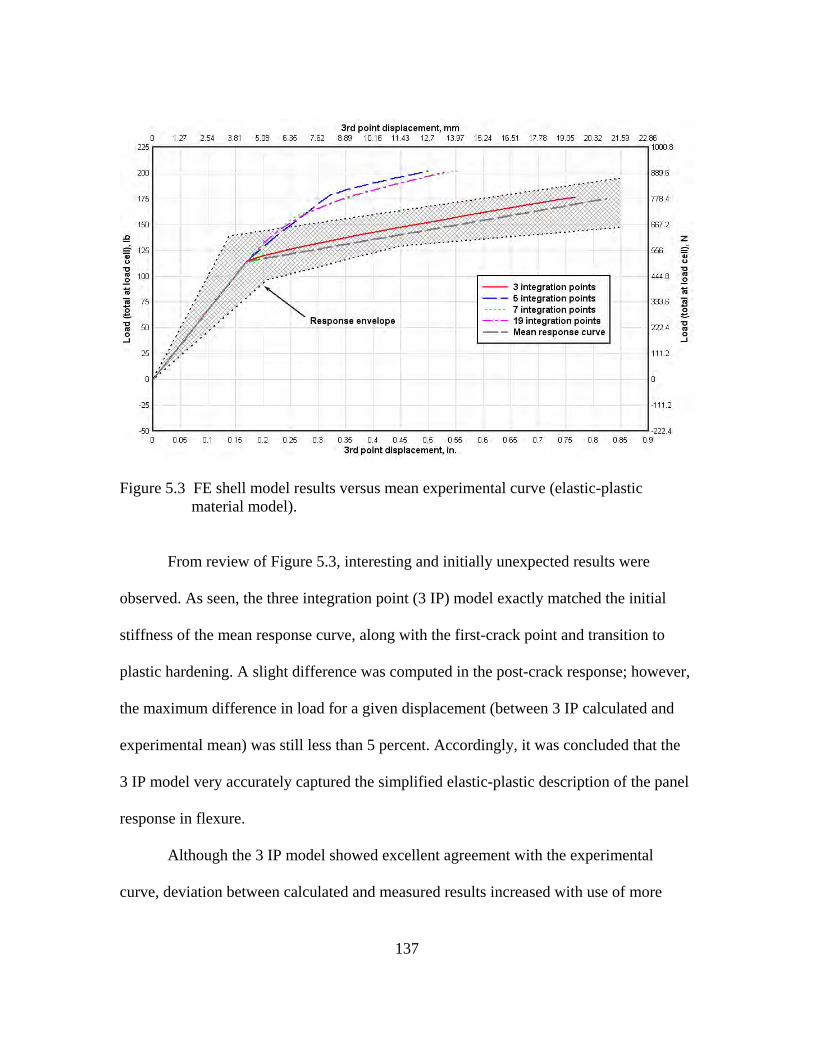
137
Figure 5.3 FE shell model results versus mean experimental curve (elastic-plastic material model).
From review of Figure 5.3, interesting and initially unexpected results were
observed. As seen, the three integration point (3 IP) model exactly matched the initial
stiffness of the mean response curve, along with the first-crack point and transition to
plastic hardening. A slight difference was computed in the post-crack response; however,
the maximum difference in load for a given displacement (between 3 IP calculated and
experimental mean) was still less than 5 percent. Accordingly, it was concluded that the
3 IP model very accurately captured the simplified elastic-plastic description of the panel
response in flexure.
Although the 3 IP model showed excellent agreement with the experimental
curve, deviation between calculated and measured results increased with use of more

138
integration points. With 5, 7, and 19 integration points, the initial linear-elastic response
exactly matched the experimental, but on reaching the first-crack strength, a gradual
transition to the defined post-crack stiffness was computed. As a result, the loads
calculated by the 5, 7, and 19 IP models for a given displacement varied from the
experimental by as much as 35 percent. Even though significant difference was observed
for the higher integration point models, once they transitioned to the plastic hardening
state, the calculated curves’ slope matched that of the 3 IP model and the experimental.
From this, it was concluded that the difference in models was a result of differences in
the transition from the elastic to plastic states.
To investigate the model’s elastic to plastic transition, stress states (in terms of the
S11 stress – reference Figure 5.1 for coordinate system orientation) for the center element
in the 3 IP and 7 IP models are given in Figures 5.4 and 5.5, respectively. Typical sign
convention is used in the plots, where tensile stress is given as positive and compressive
stress as negative.

139
Figure 5.4 3 IP stress versus load curve, center element.
Figure 5.5 7 IP stress versus load curve, center element.

140
The plots show that at an applied load of approximately 114 lb (507 N), the top
and bottom integration points for both models reached a stress of approximately 1,900 psi
(13.1 MPa), indicating that both models reached the specified cracking stress at the same
load magnitude. Therefore, the difference in load-displacement curves was not a result of
different yielding onset between the models. Although the outermost integration points in
both models reached the cracking stress at the same load magnitude, it is also seen that
the internal stress distribution differed. As will be shown, this difference in internal stress
distribution and its impact on transition to the fully plastic state was the cause of such
significant difference between the load-displacement curves.
Assuming that the difference in model responses stemmed from the internal stress
profile, the profile’s dependency on the number of integration points must be explained.
As stated previously, Simpson’s integration rule was used for the shell element
integration in all models. In ABAQUS, this results in placement of the outermost
integration points on the element top and bottom surfaces, and remaining integration
points are distributed throughout the element depth. As a result, a 3 IP model would have
one integration point on the top and bottom faces and one integration point at the
centerline. Models with a higher number of integration points would follow suit, with
additional points placed between the outer surfaces and the center. Although the
integration points are uniformly distributed, the influence area—taken as the cross-
sectional area of the element associated with a given point—are not the same. It can be
shown that for a 3 IP model, the influence area for each of the outermost integration
points is approximately 15 percent of the cross-sectional area, while the centerline point
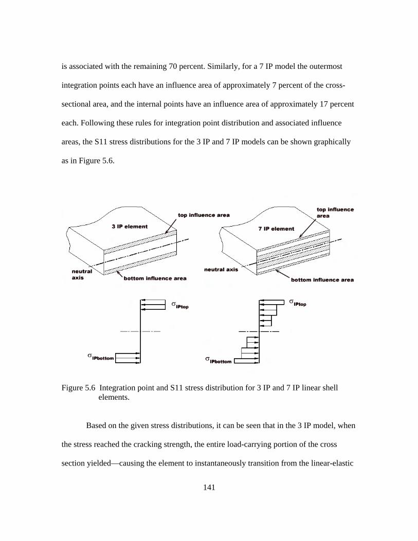
141
is associated with the remaining 70 percent. Similarly, for a 7 IP model the outermost
integration points each have an influence area of approximately 7 percent of the cross-
sectional area, and the internal points have an influence area of approximately 17 percent
each. Following these rules for integration point distribution and associated influence
areas, the S11 stress distributions for the 3 IP and 7 IP models can be shown graphically
as in Figure 5.6.
Figure 5.6 Integration point and S11 stress distribution for 3 IP and 7 IP linear shell elements.
Based on the given stress distributions, it can be seen that in the 3 IP model, when
the stress reached the cracking strength, the entire load-carrying portion of the cross
section yielded—causing the element to instantaneously transition from the linear-elastic
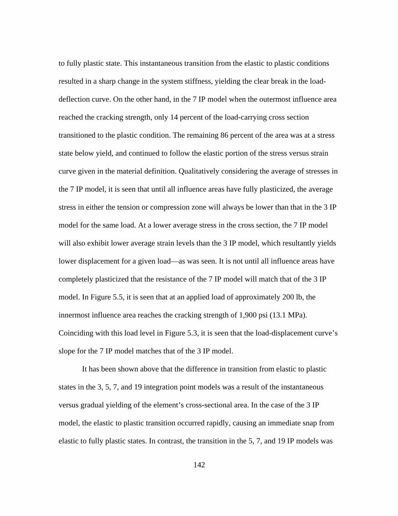
142
to fully plastic state. This instantaneous transition from the elastic to plastic conditions
resulted in a sharp change in the system stiffness, yielding the clear break in the load-
deflection curve. On the other hand, in the 7 IP model when the outermost influence area
reached the cracking strength, only 14 percent of the load-carrying cross section
transitioned to the plastic condition. The remaining 86 percent of the area was at a stress
state below yield, and continued to follow the elastic portion of the stress versus strain
curve given in the material definition. Qualitatively considering the average of stresses in
the 7 IP model, it is seen that until all influence areas have fully plasticized, the average
stress in either the tension or compression zone will always be lower than that in the 3 IP
model for the same load. At a lower average stress in the cross section, the 7 IP model
will also exhibit lower average strain levels than the 3 IP model, which resultantly yields
lower displacement for a given load—as was seen. It is not until all influence areas have
completely plasticized that the resistance of the 7 IP model will match that of the 3 IP
model. In Figure 5.5, it is seen that at an applied load of approximately 200 lb, the
innermost influence area reaches the cracking strength of 1,900 psi (13.1 MPa).
Coinciding with this load level in Figure 5.3, it is seen that the load-displacement curve’s
slope for the 7 IP model matches that of the 3 IP model.
It has been shown above that the difference in transition from elastic to plastic
states in the 3, 5, 7, and 19 integration point models was a result of the instantaneous
versus gradual yielding of the element’s cross-sectional area. In the case of the 3 IP
model, the elastic to plastic transition occurred rapidly, causing an immediate snap from
elastic to fully plastic states. In contrast, the transition in the 5, 7, and 19 IP models was

143
gradual, providing additional load carrying capacity after reaching the cracking stress at
the outermost integration points. Although for some materials, such as steel, a gradual
transition between elastic and plastic states may be appropriate, at a minimum the
experimental data for the VHSC specimens indicate that the transition is much more
abrupt. Furthermore, considering that the loss in stiffness of the VHSC material is a result
of microcrack formation, which would be expected to occur very rapidly throughout the
tension zone, the abrupt change in system stiffness could also qualitatively be expected.
Because of this, it is believed that the 3 IP model is a more accurate (albeit highly
simplified) representation of the system response to load, not only due to the excellent
match with the experimental data but also from consideration of the failure mechanisms
taking place in the cementitous material.
Recognizing that the higher integration point models only differ from the 3 IP
model in the mode of transition between elastic and plastic states, it is of interest to
determine what yield stress level would be theoretically required to match the appropriate
post-crack response. This is especially true since use of higher numbers of integration
points yields a converged solution, eliminating the dependency of the 3 IP model’s
results. To this end, the load-displacement curves given in Figure 5.3 are repeated in
Figure 5.7, but were calculated with a cracking strength of 1,100 psi (7.6 MPa) in the 5,
7, and 19 IP models. As seen, with the lower first-crack strength the higher integration
point models match the recommended response function equally well, with the exception
of transition from the elastic to plastic states.

144
Figure 5.7 FE load-deflection curves, adjusted yield stress for 5, 7, and 19 IP models.
5.2 Shell element model with concrete damage material model
The previous section showed that a basic elastic-plastic material model could be
used to calculate global load-displacement response of the panels. However, this is only
an approximating approach that predicts the overall response, without basis on the
material’s true mechanical characteristics. For example, at the yield point the elastic-
plastic model snaps both the tension and compression zones into a plastic couple of equal
magnitude, when in reality the loss of material resistance is due to strength loss in the
tensile zone and an associated climb in stress in the compression zone. Furthermore, the
elastic-plastic model gives no consideration to the material’s ultimate failure, requiring
the user to know a priori at what load or displacement final rupture will occur. Certainly,
an estimate of the ultimate displacement can be made from the experimental data

145
presented in Table 2.3 (data indicating a mean ultimate displacement of 0.541 in.
(13.7 mm)), but the capability to capture this point based on fundamental material
characteristics is far more useful. For these reasons, the shell element model used for the
elastic-plastic material study was modified to use a constitutive model expected to more
realistically represent the fundamental material characteristics.
The material model selected for use was the concrete damage plasticity model.
The damage plasticity model considers evolving compression and tension failure
surfaces, with the assumed primary purpose of modeling compressive plasticity as a
function of confining stresses. However, the model also allows for a user-specified tensile
stress versus inelastic strain (or crack opening) function, which can be used to input a
post-crack tensile softening function based on the glass fibers’ influence on failure. The
concrete damage model can be coupled with the same elastic material model used in the
elastic-plastic model; and as a result, the initial linear-elastic response description
remains unchanged.
Input for the concrete damage plasticity model is required in three general areas,
which include (a) plasticity, (b) compressive behavior, and (c) tensile behavior. The
plasticity input defines the evolving failure surfaces and plastic flow characteristics of the
concrete. Because plasticity potential in the compressive region was not considered to be
of significance in this problem, default or recommended values for the input parameters
were used. The plasticity parameters and input values included:
• dilation angle, Ψ, 1 deg
• eccentricity, ε, 0.1

146
• ratio of initial equibiaxial compressive yield stress to uniaxial compressive yield
stress, σb0/σc0, 1.16
• ratio of second stress invariant on the tensile meridian to that on the compressive
meridian, K, 0.667
• viscosity parameter, μ, 0
Detailed discussion of these plasticity parameters can be found in the ABAQUS
user’s manual.
The compressive behavior, which is the second major input requirement for the
damage plasticity model, is defined by the compressive yield stress and associated plastic
strains (if strain hardening or softening is required). In this model, the yield stress was
specified to be 21,500 psi (148 MPa) with no post-yield compressive hardening or
softening.
For this effort, the final material descriptive criteria, the tensile softening function,
was of greatest significance and was studied parametrically to determine its effect on
global response. Since the tensile failure curve definition was varied, discussion of the
input values is held for presentation in conjunction with the model results.
Building on results from the elastic-plastic model, the initial set of calculations for
the plasticity damage model was performed with 3, 7, 9, and 15 integration points, with a
tensile failure curve approximating that determined from the direct tension experiments
(reference Figure 3.38). The input tensile curve is given in Figure 5.8, along with the
recommended bridging stress function from the direct tension experiments.

147
Figure 5.8 Initial tensile failure curve definition for concrete damage model.
Using the given tensile failure curve, global response of the panel was calculated
and compared to the mean response function for each of the integration point conditions.
Results of this comparison are shown in Figure 5.9. As seen, the results are somewhat
similar to those from the elastic-plastic model, in that the 3 IP model exactly captured the
sharp material cracking point, and the higher integration point models experienced a
gradual transition to the post-crack response. The higher integration point models also
matched the post-crack system stiffness, but the 3 IP model showed a small deviation up
to an approximate 0.3 in. (7.6 mm) displacement and then exhibited greater deviation as
displacements increased.
148
Figure 5.9 Concrete damage model results for 3, 7, 9 and 15 integration points.
To determine the reason for the 3 IP model’s poor estimate of the system’s
post-crack response, the center element’s S11 stress state as a function of load was
studied. Shown in Figure 5.10, the element’s internal stress conditions initiated in similar
fashion to the elastic-plastic model, with equal stress gains at the outermost integration
points and no stress at the center point. However, on reaching the specified cracking
strength of approximately 1,900 psi (13.1 MPa), the bottom integration point began to
lose strength in accordance with the tensile failure curve, and the top integration point
began to increase in stress at a greater rate. Obviously this was a result of the different
yield stress definitions in tension and compression, and was the natural response expected
for concrete. Accompanying this loss of tensile strength was also an upward shift of the
neutral axis, which brought the center integration point into a non-zero stress state.

149
Figure 5.10 Concrete damage model, center element stress state for 3 IP model.
This shift in the neutral axis was also a naturally expected occurrence for the concrete
specimens, but was also the exact cause of subsequently erroneous post-crack stiffness in
the 3 IP model.
To further explain, as the neutral axis shifted upward, the influence area
associated with the center integration point began to contribute to the tensile component
of the element’s internal resistive couple. Recalling from Figure 5.6 the significant area
associated with the center integration point in a 3 IP model, it is apparent that the
contributing resistance could be large even with small increases in stress. Also,
considering that the integration point was initially located at the neutral axis and had only
begun to shift away from it, the associated strain was very low—corresponding to the
initial portions of linear-elastic response from the material model. Therefore, the resulting

150
condition was that after yield of the material at the outer integration point—which should
have coincided with significant loss of stiffness in the overall system—the 3 IP model
caused approximately 70 percent of the cross-sectional area to be engaged as if it were
just beginning to move up the linear-elastic stress-strain curve. As a result, the model
calculated a drastically erroneous stiffness for the system, which yielded the increase in
post-crack resistance observed in the load-deflection plot.
In the elastic-plastic model, the significant area associated with a 3 IP model’s
center integration point was not of significance because the neutral axis would not shift,
which is why it provided an excellent integration scheme when the simplified
elastic-plastic material was used. However, in the case where the neutral axis was
allowed to shift the 3 IP model provided the worst integration scheme by far, essentially
inhibiting the progressive tensile failure that should naturally take place in the cross
section. For this reason, in the concrete damage model the higher integration point
models provided the best choice of integration schemes, with convergence observed for
seven integration points. Notably, this is in agreement with commentary given in the
ABAQUS user’s manual, which states that seven or more integration points should be
used when the concrete damage model is implemented with shell elements such that
progressive failure of the tensile zone can be captured.
Recognizing that the 7 IP model provides the best integration scheme for use with
the concrete damage material model, the discrepancy between experimental first-crack
load (113 lb (503 N)) and peak load after the model’s full transition to the post-crack
stiffness (155 lb (689 N)) must be addressed. With the elastic-plastic material model, the
151
higher integration point models were matched to the experimental data simply by
specifying a lower cracking strength. The lower strength value, 1,100 psi (7.6 MPa), was
selected in the elastic-plastic model iteratively, by means of determining the best match
to the experimental data. However, when coupling this correction with the bridging
function given in Figure 5.8, it is recognized that more significant meaning was
associated with the 1,100 psi (7.6 MPa) stress level.
Recalling discussion of the recommended bridging function in Chapter 3, it was
noted that the peak stress of approximately 2,000 psi (13.8 MPa) represents the
cementitous matrix failure point, marking the initiation of microcrack formation
throughout the matrix and the onset of brittle tensile failure in the section. However, as
the material’s strength rapidly drops, at approximately 1,100 psi (7.6 MPa) the fibers
become engaged and provide bridging capacity at the cracks—resulting in increased
ductility for the remainder of response. With this analysis of the bridging function in
mind, it is seen that the correction required for the higher integration point models is to
disregard that portion of the bridging stress function associated with the transition from
brittle failure of the matrix to ductile response induced by the bridging fibers. In other
words, because the higher integration point models cannot capture the instantaneous
tensile failure throughout the cementitous matrix—which brings about the sharp
transition from pre- to post-crack stiffness—then the tensile failure function in the
numerical model should only be defined by the fiber-enhanced ductile portion of the
curve—which brings about the post-crack stiffness.

152
The above considered, the tensile failure function given in Figure 5.8 was
truncated to a peak stress of 1,100 psi (7.6 MPa), as shown in Figure 5.11. With the
revised definition of post-crack response, the 7 IP model was run again for comparison to
the experimental curve. The results are shown in Figure 5.12.
Figure 5.11 Truncated tensile failure curve definition for concrete damage model.

153
Figure 5.12 Concrete damage model results with truncated tensile failure function.
As was expected, truncation of the brittle matrix failure component from the
tensile failure function resulted in much better agreement between the numerical model’s
post-crack stiffness and the experimentally determined curve. The match was not exact
between experimental and calculated; however, considering that the post-crack response
was calculated solely from the tensile failure function, with no direct input of the
measured post-crack stiffness, the results are considered to be fairly good.
Although reasonably matching the post-crack portion of the load-displacement
curve, the model did not capture the panel’s ultimate failure, which was a primary reason
for using the concrete damage material model. In this case, the calculations were
automatically stopped because of an excessively small arc length, indicating that the Riks
analysis could not find a solution. Presumably, this occurred because of the calculated

154
load-displacement curve’s flatness, which was approaching near zero stiffness in the
system. For further insight into the calculated panel response, S11 stress states at the
center element’s integration points were plotted, and are given in Figure 5.13.
Figure 5.13 Center element S11 stress states, concrete damage model with truncated tensile failure function.
Figure 5.13 shows that the integration points progressively transitioned into the
tensile failure phase of response, as was expected. At conclusion of the calculation, five
out of the seven integration points were strained in tension, and four of them had reached
the cracking strength and were following the defined tensile failure function. Although
four of the integration points had theoretically “failed” in tension, it is seen in the figure
that they had not experienced significant strength loss at the calculation’s conclusion.
Rather, they showed only small changes in strength, most noticeably observed for the

155
bottom integration point, which dropped in strength from approximately 1,100 psi
(7.6 MPa) at tensile failure initiation to 980 psi (6.7 MPa). Referencing Figure 5.11, this
indicates that the crack width was approximately 0.001 in. (0.02 mm), although the
calculated third-point deflection was near 0.65 in. (16.5 mm). From Table 2.3, the
experimental data showed a mean third-point deflection at ultimate failure of 0.54 in.
(13.7 mm), and it was subsequently concluded that for the given model formulation, the
specified tensile failure function provided too much resistance into the system—resulting
in the extended post-crack response.
Following the observations above, a set of iterative calculations were conducted
to evaluate the influence of certain aspects of the tensile failure function. From this
exercise, it was found that the global system stiffness and resulting initiation of ultimate
failure were highly dependent on even small changes in the tensile failure function. Two
revised failure functions evaluated in the iterative calculations are given in Figure 5.14,
and their associated load-displacement curves are given in Figure 5.15. Since capture of
the ultimate failure point is of interest in these calculations, instead of comparison to the
mean response function, numerical results are directly compared to the individually
measured load-displacement curves for each test.

156
Figure 5.14 Revised tensile failure functions from iterative calculations.
Figure 5.15 Third-point displacement comparison, computed versus experimental
(concrete damage material model).

157
From Figure 5.15, with the given tensile failure definitions the numerical model
closely matched all aspects of the experimentally observed panel response. As with
previous calculations, the elastic portion of the material definition results in a
linear-elastic load-displacement response that exactly follows the mean of the
experimental data. Furthermore, the computed post-crack stiffness is very close to the
experimental, with the Curve A definition providing somewhat better results than
Curve B. Of greatest significance from these data is capture of the ultimate failure of the
panels, both with respect to ultimate displacement and the trend of the post-failure curve.
Both tensile failure definitions calculated a sharp failure point after some amount of post-
crack displacement, just as was observed experimentally. Furthermore, the models also
calculated a small amount of residual, reduced capacity after panel rupture, very similar
to the response seen in Tests 6, 8, and 9. From these results, it was concluded that within
the context of the still simplified approach to calculation of the complex fracture
mechanics taking place in the concrete panels, the concrete damage material model,
coupled with the experimentally determined tensile failure criteria, provided a very good
tool for calculation of the thin panel response.
Having made the above statements regarding the quality of model results and their
validity in calculating the panel response, it is also acknowledged that to obtain these
results the required tensile failure functions are similar in shape to the experimental data,
but also possess less fracture energy (defined as area under the tensile failure curve). The
reason for this is not known, but likely stems from simplicity in approach of using a basic
tensile failure function to describe the complex fracture event. However, because the

158
nature of the numerical failure curves generally match the experimental, it is believed that
factors controlling the calculated response are the same as those governing the real panel
resistance to load. Because of this, the model provides significant usefulness in future
analysis of the panel response, simply by understanding the basic influence of changes in
the tensile failure curve on the global panel response.
For example, in the micromechanical model analyses given in Chapter 3, it was
concluded that the flat portion of the tensile failure function at approximately 1,100 psi
(7.6 MPa) (reference Curve A) occurred as the fibers were engaged and began their
debonding process. From these numerical analyses, it was seen that this flat portion of the
curve also directly influenced the magnitude of post-crack displacement occurring before
ultimate failure in the panel. Therefore, it can be concluded that energy absorption during
debonding of the glass fibers has a significant impact on the thin VHSC panels, and
further enhancement of ductility could be gained by manipulation of this effect. The same
type of analysis can be conducted for other portions of the curve—relating global
response to the physical meaning of the tensile failure function—providing potential for
other engineered improvements of the panel response.

159
CHAPTER VI
SUMMARY AND CONCLUSIONS
6.1 Summary
The purpose of this research was to characterize the flexural and tensile properties
of 0.5-in.-thick (12.7-mm), ultra-high performance concrete panels developed by the U.S.
Army Engineer Research and Development Center (ERDC). The panels, developed by
ERDC for special applications of military interest, were made with a unique cementitous
mix, such that compressive strengths of 21,500 psi (148 MPa) or greater were obtained.
Because of the minimal thickness desired for the panels, conventional reinforcing could
not be incorporated to provide tensile capacity in the material. Therefore, the panels were
reinforced solely with discontinuous, alkali-resistant fiberglass fibers chopped to a length
of 1 in. (25.4 mm) and incorporated into the panels at a loading rate of 3 percent by
volume.
Laboratory experiments, micromechanically based analytical models, and
numerical models were used to study the material and characterize the panels’ response
to load. Experimentation included third-point bending tests conducted in accordance with
ASTM C947-03 and novel direct tension tests patterned after similar research efforts
published in the literature. Analytical study of the material’s tensile characteristics was
largely based on a body of work published by Victor C. Li, E.B. Wylie Collegiate Chair
at the University of Michigan, Ann Arbor, and noted authority in the field of

160
fiber-reinforced concrete. Implementation of Li’s work followed a progressive
development of the micromechanically based analytical models, beginning with
development of a single fiber pullout model, and then building to more complex
considerations such as fiber rupture and slip softening after pullout initiation. Numerical
simulations were performed with the commercial finite element code ABAQUS, and
calculations were conducted to study both the third-point bending experiments and the
direct tension tests.
6.2 Results and conclusions
The third-point bending experiments showed that the panels typically exhibited
three distinct phases of flexural response. In load-displacement space, initial response
was observed to be highly linear, up to a first-crack load between 100 lb (444 N) and
125 lb (556 N). The mean modulus calculated for the linear-elastic response was 5.7×10⁶
psi (39.3 GPa), with a mean cracking strength of 1,887 psi (13 MPa). At conclusion of
the linear-elastic response, the panels sharply transitioned into a softened response state,
characterized again by a fairly linear load-displacement relationship, which progressed to
the point of ultimate load. The mean load capacity increase between first-crack and
ultimate failure was approximately 35 percent of the first-crack load, and the mean
softened modulus was calculated to be 0.79×10⁶ psi (5.4 GPa). On reaching ultimate
load, the panels generally failed abruptly with formation of a single macrocrack and a
rapid loss of load resistance. In some cases (30 to 40 percent of the panels), a small
residual load-carrying capacity was observed after ultimate failure, with the residual
capacity being approximately 15 to 20 percent of the ultimate load. Defining toughness as

161
the area under the load-displacement curves, and assuming that unreinforced panels
would have completely failed at conclusion of the initial linear-elastic response, the data
showed that inclusion of fiberglass fibers increased the panel toughness between 300
percent and 1,000 percent. The wide range of toughness enhancement was a result of the
high variability observed in the panel’s ultimate displacement at peak load, which ranged
from 0.27 in. (6.8 mm) to 0.83 in. (21 mm).
The direct tension experiments were much more limited in scope as compared to
the bending tests, and were primarily conducted to gather representative tensile response
data supportive to the other project components. With foil strain gages mounted to the
specimens at multiple locations, the data gave insight to the material’s initial linear
modulus, the strain recovery in the uncracked sections, and the post-crack tensile
softening response at the crack location. The calculated initial modulus closely agreed
with that from the bending experiments, with a mean value of 6.1×10⁶ psi (42.0 GPa).
Furthermore, data from the uncracked sections validated that the initial modulus was not
only linear but also elastic, with the majority of strain recovered after crack formation at
the notch. Finally, data from gages at the specimen notch indicated that in the
fiber-reinforced material, the crack growth was characterized by a gradually softening
tensile failure curve. The softening function was initiated at a calculated cross section
stress of approximately 1,100 psi (7.6 MPa), and fell to less than 100 psi (0.7 MPa) at a
crack opening width of approximately 0.025 in. (0.63 mm). Although the softening
function was initiated at 1,100 psi (7.6 MPa), analysis of the data indicated that, due to
stress concentration at the notch, the specimens’ true peak stress was closer to 2,000 psi

162
(13.8 MPa). It was concluded that the cementitous matrix ruptured in a brittle mode at
approximately 2,000 psi (13.8 MPa), at which point strength dropped rapidly until the
fibers were engaged at approximately 1,100 psi (7.6 MPa). After fiber engagement the
response was more ductile, as previously discussed.
The micromechanically based analytical models were primarily used to study the
mesoscale phenomena driving the macroscale tensile softening response. At conclusion
of the calculations, model results did not yield exact matches to the direct tension
experimental data—likely due to the lack of exact micromechanical properties such as the
glass fiber interfacial bond strength. However, sufficient similarity was present to make
postulations of the underlying mechanics driving the material’s macroscopic
performance.
The first model analysis, based solely on a fiber pullout mode of failure (no
consideration of fiber rupture), validated conclusions from the direct tension data
regarding transition from the peak matrix stress to the stress at full fiber engagement. In
the pullout only model, it was shown that assuming a reasonable interfacial bond strength
value, the maximum bridging stress that could be developed by the fibers was close to
1,100 psi (6.9 MPa). Having given the argument that transition from maximum matrix
stress to the maximum fiber bridging stress occurs rapidly (reference discussion in
Section 4.3), this indicated that initial tensile response of the material would be just as
shown in the direct tension test data’s recommended bridging stress function—
characterized by a sharp drop in strength from the peak matrix stress to the peak fiber
bridging strength.

163
On reaching the peak fiber bridging strength, the model showed that initial fiber
response was governed by a debonding phase, where the slip zones were formed between
the fibers and the matrix. Depending on fiber and matrix characteristics, this debonding
phase could occur over a range of crack opening widths, giving rise to different shapes of
the tensile failure curve at the 1,100 psi (7.6 MPa) stress level. With sufficient debonding
resistance, the tensile failure curve could have a flat portion as seen in direct tension
Test 2. Otherwise, the curve would immediately progress to the softening failure as seen
in direct tension Test 1.
Because fiber rupture was observed in the laboratory specimens, a second
formulation of the micromechanical model was studied to consider rupture effects. The
model indicated that fiber rupture would generally result in specimen response similar to
that observed, marked by a sharp strength drop as the fibers failed in a brittle mode.
However, based on fiber properties the model also showed that to induce rupture under
pure axial load, the interfacial bond strength must be factors larger than assumed for the
pullout model (close to 5,000 psi (34.4 MPa)). As a result, the overall tensile failure
function for the material would be significantly greater than that measured, and it was
concluded that fiber rupture was not a significant contributor to the observed macroscopic
material performance. The fiber rupture failures observed in the laboratory specimens
were more likely a result of bending failure rather than rupture in pure tension, which is a
glass fiber failure mode documented in the literature.
The final aspect of tensile failure response studied with the micromechanical
models was the post-debonding, fiber pullout phase. The basic pullout model assumed

164
constant, frictional interfacial bond strength between the fiber and matrix. However, this
assumption resulted in a generally linear drop in fiber bridging strength up to a maximum
crack opening width of 0.5 in. (12.7 mm). This greatly differed from the experimental
data, in which the maximum crack opening width was only 0.025 in. (0.63 mm).
Therefore, the potential for slip-softening between the fibers and matrix was considered;
and with a strong exponential decay assumed for the softening function, the model’s
pullout phase of response more closely matched the experimentally measured. Although
slip-softening pullout provided a relatively close match to the experimental response, it
should be noted that this assumed a friction-controlled pullout mode. It is also possible
that the fiber-matrix bond was chemically governed. Based on the estimated interfacial
bond strength (approximately 1,500 psi (10.3 MPa)) and the strong pullout decay, it is
possible that the bond between fiber and matrix was more chemically than mechanically
driven. As documented for PVA fibers, chemical bond could result in elevated interfacial
bond strengths; and since the chemical bond would effectively fall to zero at failure, the
slip strength would fall rapidly as appeared to be the case in the data.
In the numerical modeling portion of the project, two material model formulations
were coupled with a shell element FE model to simulate panel response in third-point
bending. The first material model was elastic-plastic with strain hardening, which was
based on the simple dual-stiffness description of model response given by the
experimentally measured mean response function (reference Figure 2.18). Results
showed that with assumed pre- and post-crack modulii of 5.7×10⁶ psi (39.3 GPa) and
0.79×10⁶ psi (5.4 GPa), respectively, the model was capable of exactly matching the

165
experimental curve. Although capable of providing a good match to the
load-displacement data, it was also found that the shell model results were subject to
integration point dependency. From a convergence study of through-the-thickness
integration points, it was observed that a three integration point model provided a sharp
transition from pre- to post-crack states just as was seen in the experimental data.
However, when higher numbers of integration points were used, the transition was more
gradual, and resulted in an overestimation of the cracking strength. It was shown that this
difference was a result of integration point distribution through the element thickness,
and it was concluded that the three integration point model yielded the most realistic
description of physical panel response.
Although the dependency study yielded interesting results regarding the best
integration scheme from a numerical perspective, of greater interest was the observed
correlation between the integration point dependent response and the material’s
mechanical properties. It was shown in the direct tension experiments that the material
exhibited a near instantaneous transition from matrix cracking stress of approximately
2,000 psi (13.8 MPa) to the fiber bridging strength of 1,100 psi (7.6 MPa). This
immediate drop in strength resulted in the flexural response’s sharp break from pre-
to post-crack stiffness. Because of the integration point distribution in the three-point
scheme, it was shown that on yield the model exhibited an immediate transition in
stiffness, and therefore with a first-crack strength definition of 2,000 psi (13.8 MPa)
could exactly match the experimental curve. The correlation between numerical and
experimental response was therefore the instantaneous transition of the FE section from

166
linear-elastic stiffness to the post-crack stiffness, as occurred with brittle failure of the
cementitous matrix. However, with a higher number of integration points, the elements
could not snap from elastic to plastic phases, not capable of capturing the rapid cracking
failure occurring throughout the brittle cementitous material. For this reason, it was
necessary to define the cracking strength in the higher integration point models as
approximately 1,100 psi (7.6 MPa), corresponding to the peak fiber bridging strength.
With this lower first-crack definition, the higher integration point models were able to
exactly match the load-displacement curve’s post-crack slope, although missing the sharp
transition from pre- to post-crack response.
Following the elastic-plastic material model implementation, a concrete damage
model was used to provide a more explicit definition of the tensile failure curve. This was
desired so that more direct correlation between flexural and tensile response could be
incorporated into the model, and so that ultimate failure could be captured—which was
not possible with the elastic-plastic model. Results showed that with a tensile failure
function of similar form to the experimentally measured, the damage model captured the
post-peak system stiffness with reasonable accuracy.
As with the elastic-plastic model, integration point dependency was observed, but
instead of the three integration point model providing better results, in this case seven or
more integration points were recommended. This was because of the damage model’s
capability to simulate shifting of the neutral axis, which required a more progressive
description of the cross section tensile failure. Since the higher integration point models
required a cracking strength definition to coincide with the maximum fiber bridging

167
stress (instead of the higher matrix cracking stress), they did not capture the sharp break
in load-displacement response at the yield point.
The greatest benefit of the damage model was that it showed capability to capture
ultimate failure point of the panels, without a priori knowledge of the failure
displacement or load. This is of significance in that it provides capability to study the
macroscopic influence of changes in the tensile function. Furthermore, using results of
the micromechanical model to correlate changes in the tensile failure function to basic
changes in the material’s mesoscale interaction, by extension, comprehensive design and
analysis of the panel response can be conducted.
For completeness in the project analysis, it is acknowledged that although the
damage model was able to accurately capture the global panel response, it was not based
on direct input of the measured tensile failure function. Rather, functions with less
resistance to crack opening—but with similar shape to the experimental—were required.
Although this was the case, similarities in shape indicated that the numerical model
response was a function of the basic physical properties governing the experimental
function, and therefore the capability to conduct future material engineering and analysis
is still supported.
6.3 Recommended panel and material properties
Considering that the primary purpose of this research was to determine key
flexural and tensile properties of the VHSC material and hardened 0.5-in.-thick
(12.7-mm) panels, a summary of the research findings are given below. Table 6.1
provides a summary of the determined panel and material characteristics, and Figures 6.1

168
and 6.2 provide the panel’s resistance function in third-point bending and the material’s
recommended tensile failure function, respectively.
Table 6.1
Recommended panel and material properties
Property Value material properties
linear-elastic tensile modulus, psi (GPa) 6×10⁶ (41.4) post-crack modulus, psi (GPa) 0.8×10⁶ (5.5)
matrix cracking stress, psi (MPa) 2,000 (13.8) maximum fiber bridging strength, psi (MPa) 1,100 (7.6)
fiber/matrix interfacial bond strength, psi (MPa) 600 (4.1) to 1,400 (9.6) panel properties1
first-crack load2, lb (N) 115 (502) ultimate load2, lb (N) 150 (667)
first-crack displacement at third-point, in. (mm) 0.18 (4.6) ultimate displacement at third-point, in. (mm) 0.54 (13.7)
1 based on third-point bending with a 10-in. (254-mm) wide panel on a 36-in. (914-mm) span
2 total load applied to panel; one-half at each third-point

169
Figure 6.1 Recommended load-displacement resistance function (third-point loading,
10-in.-wide panel, 36-in. span).
Figure 6.2 Recommended tensile failure function (crack bridging stress function).

170
6.4 Recommendations for future research
Through this research program, a basic study was conducted on the hardened
properties and mesoscale mechanics of ERDC’s newly developed VHSC panels.
Providing a thorough investigation of the material’s basic characteristics, the effort also
provided a foundation for future work by identifying areas in which additional research
could be used to extend the current findings. A primary area recommended for future
study is the direct tension experiments. Because of limited resources, only a small
number of experiments could be conducted in this program. However, as observed with
the flexural tests, the VHSC material inherently possesses a stochastic nature that gives
rise to a certain amount of variability in any of its mechanical characteristics. Considering
that the thin panel’s response to load will be completely governed by its tensile softening
characteristics in most all expected applications, more thorough experimental
examination of this property is warranted.
In addition to further direct tension testing, mesoscale experimentation should
also be considered as an area of future research. The micromechanical analyses showed
that the macroscopic material performance can be linked to the mesoscale mechanics.
However, based on a lack of basic mesoscale material parameters, the micromechanical
models showed only limited capability in truly analyzing response. Therefore, with
additional experimentation such as single fiber pull tests, nanoindentation, and electron
microscope examination of the fiber/matrix interfacial transition zone, the
micromechanical analyses could be made much more effective in understanding
macroscopic response. Furthermore, with in-depth understanding of the mesoscale

171
phenomenon the material could be better engineered in terms of its tensile softening
capability (via fiber hybridization, manipulation of fiber geometry, changes in fiber
volume fraction, etc.), so that it could show even greater improvements in ductility, and
perhaps make more effective use of its high compressive strength in a structural sense.
Lastly, under future efforts the numerical models might be extended from the
basic homogenized material models used in this program, to application of the state-of-art
models currently being developed by Z. Bazant [41], P. Kabele [42-45], G. Cusatis
[59-61], and others. Furthermore, advanced numerical methods, such as the meshless,
reproducing kernel particle method (RKPM) being developed by J.S. Chen [62, 63] could
also be applied to study the material at multiple length scales and under a vast array of
loading conditions.

172
BIBLIOGRAPHY
1. van Mier, Jan G.M. (1997). “Fundamental aspects of mechanical behaviour of HS/HPC: The European approach,” High Strength Concrete – First International Conference. Kona, HI, July 13-18, 1997. A. Atorod, D. Darwin, and C. French, eds., ASCE, Reston, VA, 457-469.
2. Chanvillard, G. and Rigaud, S. (2003). “Complete characterisation of tensile properties of Ductal® UHPFRC according to the French recommendations,” Fourth International Workshop on High Performance Fiber Reinforced Cement Composites (HPFRCC4). Ann Arbor, MI, June 15-18, 2003. RILEM Publications, A.E. Naaman and H.W. Reinhardt, eds., Bagneux, France, 21-34.
3. O’Neil, E.F., Neeley, B.D., and Cargile, J.D. (1999). “Tensile properties of very-high-strength concrete for penetration-resistant structures,” Shock and Vibration 6, 237-245.
4. O’Neil, E.F., III, Cummins, T.K., Durst, B.P., Kinnebrew, P.G., Boone, R.N., and Toores, R.X. (2004), “Development of very-high-strength and high-performance concrete materials for improvement of barriers against blast and projectile penetration,” U.S. Army Science Conference. Orlando, FL, December 2004.
5. Shah, S.P. (1997). “Material aspects of high performance concrete,” High Strength Concrete – First International Conference. Kona, HI, July 13-18, 1997. A. Atorod, D. Darwin, and C. French, eds., ASCE, Reston, VA, 504-516.
6. Watanabe, F. (1997). “Research activities on high strength concrete and its application in Japan,” High Strength Concrete – First International Conference. Kona, HI, July 13-18, 1997. A. Atorod, D. Darwin, and C. French, eds., ASCE, Reston, VA, 636-653.
7. Bindiganavile, V., Banthia, N., and Aarup, B. (2002). “Impact response of ultra-high-strength fiber-reinforced cement composite,” ACI Materials Journal, V. 99, No. 6, 543-548.
8. Ngo, T., Mendis, P., Lam, N., and Cavill, B. (2005). “Performance of ultra-high strength concrete panels subjected to blast loading.” Science, engineering and technology summit. Canberra, Australia, 2005. P. Mendis, J. Lai, and E. Dawson, ed., Research Network for a Secure Australia, 193-208.

173
9. ACI Committee 549 (2004). “Report on thin reinforced cementitous products,”
ACI 549.29-04, American Concrete Institute, Farmington Hills, MI.
10. ACI Committee 544. (1996). “Report on fiber reinforced concrete,” ACI 544.1R-96, American Concrete Institute, Farmington Hills, MI.
11. Luo, X., Sun, W., and Chan, S.Y.N. (2000). “Steel fiber reinforced high-performance concrete: a study on the mechanical properties and resistance against impact,” Materials and Structures, V. 34, 144-149.
12. Shah, S. (1991). “Do fibers increase the tensile strength of cement-based
matrixes?” ACI Materials Journal, V. 88, No. 6, 595-602.
13. ACI Committee 549 (1993, reapproved 1999). “Guide for the design, construction and repair of ferrocement,” ACI 549.1R-93, American Concrete Institute, Farmington Hills, MI.
14. ACI Committee 544 (1988, reapproved 1999). “Design considerations for steel fiber reinforced concrete,” ACI 544.4R-88, American Concrete Institute, Farmington Hills, MI.
15. Balaguru, P., Narahari, R., and Patel, M. (1992). “Flexural toughness of steel fiber reinforced concrete,” ACI Materials Journal, V. 89, No. 6, 541-546.
16. Biolzi, L., Cattaneo, S., and Labuz, J.F. (2001). “Tensile and bending tests on very high performance concrete.” Fracture Mechanics for Concrete Materials: Testing and Applications. C. Vipulanandan and W.H. Gerstle, ed., ACI Special Publication 201, 229-242.
17. Giaccio, G., and Zerbino, R. (2002). “Fiber reinforced high strength concrete: evaluation of failure mechanism.” High Performance Concrete, Performance and Quality of Concrete Structures (Proceedings, Third International Conference, Recife, PE, Brazil). V.M. Malhotra, P. Helene, E.P. Figueirdo, and A. Carneiro, ed., ACI Special Publication 207, 69-89.
18. Mobasher, B., and Shah, S.P. (1989). “Test parameters for evaluating toughness of glass-fiber reinforced concrete panels,” ACI Materials Journal, V. 86, No. 5, 448-458.

174
19. Banthia, N. and Gupta, R. (2004). “Hybrid fiber reinforced concrete (HyFRC):
fiber synergy in high strength matrices,” Materials and Structures, V. 37, 707-716.
20. Wang, Y., Li, V. C., Backer, S. (1991) “Tensile failure mechanism in synthetic fibre-reinforced mortar,” Journal of Materials Science, V. 26, 6565-6575.
21. Wang, Y., Backer, S., and Li, V. C. (1989). “A statistical tensile model of fibre reinforced cementitious composites,” Composites, V. 20, No. 3, 265-274.
22. Leung, C. K. Y., and Li, V. C. (1991). “New strength-based model for the debonding of discontinuous fibres in an elastic matrix,” Journal of Materials Science, V. 26, 5996-6010.
23. Li, V. C., Wang, Y., and Backer, S. (1991). “A micromechanical model of tension-softening and bridging toughening of short random fiber reinforced brittle matrix composites,” J. Mech. Phys Solids, V. 39, No. 5, 607-625.
24. Li, V. C. (1992). “Postcrack scaling relations for fiber reinforced concrete cementitous composites,” Journal of Materials in Civil Engineering, V. 4, No. 1, 41-57.
25. Wu, H., and Li, V. C. (1994). “Trade-off between strength and ductility of random discontinuous fiber reinforced cementitous composites,” Cement and Concrete Composites, V. 16, 23-29.
26. Li, V. C., Stang, H, and Krenchel, H. (1993). “Micromechanics of crack bridging in fibre-reinforced concrete,” Materials and Structures, V. 26, 486-494.
27. Li, V. C., Maalej, M., and Hashida, T. (1994). “Experimental determination of the stress-crack opening relation in fibre cementitious composites with a crack tip singularity,” Journal of Materials Science, V. 29, 2719-2724.
28. Obla, K. H. and Li, V. C. (1995). “A novel technique for fiber-matrix bond strength determination for rupturing fibers,” Cement and Concrete Composites, V. 17, 219-227.

175
29. Stang, H., Li, V. C., and Krenchel, H. (1995). “Design and structural application
of stress-crack width relation in fibre reinforced concrete,” Materials and Structures, V. 28, 210-219.
30. Maalej, M., Li, V. C., and Hashida, P. (1995). “Effect of fiber rupture on tensile properties of short fiber composites,” Journal of Engineering Mechanics, V. 121, No. 8, 903-913.
31. Li, V. C. and Maalej, M. (1996). “Toughening in cement based composites. Part II: fiber reinforced cementitous composites,” Cement and Concrete Composites, V. 18, 239-249.
32. Li, V. C., Wu, H., Maalej, M., Mishra, D. K., and Hashida, T. (1996). “Tensile behavior of cement-based composites with random discontinuous steel fibers,” Journal of the American Ceramic Society, V. 79, No. 1, 74-78.
33. Li, V. C., and Stang H. (1997). “Interface property characterization and strengthening mechanisms in fiber reinforced cement based composites,” Advanced Cement Based Materials, V. 6, 1-20.
34. Li, V. C., Lin, Z., and Matsumoto, T. (1998). “Influence of fiber bridging on structural size-effect,” Int. J. Solids Structures, V. 35, Nos. 31 and 32, 4223-4238.
35. Li, V. C., and Wang, S. (2006). “Microstructure variability and macroscopic composite properties of high performance fiber reinforced cementitious composites,” Probabilistic Engineering Mechanics, V. 21, 201-206.
36. Kanda, T., and Li, V. C. (1999). “Effect of fiber strength and fiber-matrix interface on crack bridging in cement composites,” Journal of Engineering Mechanics, V. 125, No. 3, 290-299.
37. Kanada, T., Lin, Z., and Li, V. C. (2000). “Tensile stress-strain modeling of pseudostrain hardening cementitous composites,” Journal of Materials in Civil Engineering, V. 12, No. 2, 147-156.
38. Nelson, P. K., Li, V. C., and Kamada, T. (2002). “Fracture toughness of microfiber reinforced cement composites,” Journal of Materials in Civil Engineering, V. 14, No. 5, 384-391.

176
39. Bazant, Z.P., Xiang, Y., and Prat, P. (1996). “Microplane model for concrete.
I: stress-strain boundaries and finite strain,” Journal of Engineering Mechanics, V. 122, No. 3, 245-254.
40. Bazant, Z.P., Xiang, Y., Adley, M., Prat, P., and Akers, S. (1996). “Microplane model for concrete. II: data delocalization and verification,” Journal of Engineering Mechanics, V. 122, No. 3, 255-262.
41. Beghini, A., Bazant, Z.P., Zhou, Y., Gouirand, O., and Caner, F. (2007). “Microplane model M5f for multiaxial behavior of and fracture of fiber-reinforced concrete,” Journal of Engineering Mechanics, V. 133, No. 1, 66-75.
42. Kabele, P. (2002). “Equivalent continuum model of multiple cracking,” Engineering Mechanics (Association for Engineering Mechanics, Czech Republic), Vol. 9, 75-90.
43. Kabele, P. (2003). “New developments in analytical modeling of mechanical behavior of ECC,” Journal of Advanced Concrete Technology, V. 1, No. 3, 253-264.
44. Kabele, P. (2004). “Linking scales in modeling of fracture in high performance fiber reinforced cementitous composites,” unpublished lecture, Vail, CO, April 12-16, 2004.
45. Kabele, P. (2007). “Multiscale framework for modeling of fracture in high performance fiber reinforced cementitous composites,” Engineering Fracture Mechanics, Vol. 74, 194-209.
46. Ghoniem, N.M., Busso, E.P., Kioussis, N., and Huang, H. (2003). “Multiscale modeling of nanomechanics and micromechanics: an overview,” Philosophical Magazine, Vol. 83, Nos. 31-34, 3475-3528.
47. ASTM C 947, “Test method for flexural properties of thin-section glass-fiber reinforced concrete (using simple beam with third-point loading).”
48. Beer, F.P. and Johnston, E.R. Jr. (1992). Mechanics of Materials, second edition. McGraw-Hill, Inc., New York.

177
49. Wang, Y., Li, V. C., and Backer, S. (1990). “Experimental determination of
tensile behavior of fiber reinforced concrete,” ACI Materials Journal, V. 87, No. 5, 461-468.
50. Zheng, W., Kwan, A.K.H., and Lee, P.K.K. (2001). “Direct tension test of concrete,” ACI Materials Journal, V. 98, No. 1, 63-71.
51. ABAQUS/CAE, Version 6.5-4. (2005). SIMULIA, Providence, RI.
52. Akers, S.A., Green, M. L., and Reed, P.A. (1998). “Laboratory characterization of very high-strength fiber-reinforced concrete,” Technical report SL-98-10, U.S. Army Corps of Engineers, Waterways Experiment Station, Vicksburg, MS.
53. Zhang, J., and Li, V. C. (2002). “Effect of inclination angle on fiber rupture load in fiber reinforced cementitious composites,” Composites Sciences and Technology, V. 62, 775-781.
54. Li, V. C., Wang, Y., and Backer, S. (1990). “Effect of inclining angle, bundling, and surface treatment on synthetic fibre pull-out from a cement matrix,” Composites, V. 21, No. 2, 132-140.
55. Bentur, A., Wu, S.T., Banthia, N., Baggott, R., Hansen, W., Katz, A., Leung, C.K.Y., Li, V.C., Mobasher, B., Naaman, A.E., Robertson, R., Soroushian, P., Stang, H., and Taerwe, L.R., (1995). In High Performance Fiber Reinforced Cementitous Composites, Naaman, A.E., Reinhardt, H., eds., Chapman and Hall: London, 149-191.
56. Bentur, A. (1989). In Materials Science of Concrete, Vol. I, Skalny, J., ed., The American Ceramic Society, Inc., Westerville, OH, 223-284.
57. Gray, R., and Johnston, C.D. (1978). In Proceedings RILEM Symposium, Lancaster, 317-328.
58. Stang, H. (1995). In Fracture of brittle, disordered materials: concrete, rock and ceramics. Baker, G., Karihaloo, B.L., eds., E&FN Spoon: London, 131-148.
59. Cusatis, G., and Cedolin, L. (2006). “Two scale analysis of concrete fracturing behavior,” Engineering Fracture Mechanics, V. 74, 3-17.

178
60. Cusatis, G., Bazant, Z.P., and Cedolin, L. (2003). “Confinement-shear lattice model for concrete damage in tension and compression. II: Numerical implementation and validation,” Journal of Engineering Mechanics, ASCE, V. 129, No. 12, 1449-1458.
61. Cusatis, G., Bazant, Z.P., and Cedolin, L. (2003). “Confinement-shear lattice model for concrete damage in tension and compression. I: Theory,” Journal of Engineering Mechanics, ASCE, V. 129, No. 12, 1439-1448.
62. Chen, J.S., Pan C., Wu, C.T., and Liu, W.K. (1996). “Reproducing kernel particle methods for large deformation analysis of non-linear structures,” Computer Methods in Applied Mechanics and Engineering, V. 139, 195-227.
63. Chen, J.S., Pan, C., Roque, C., and Wang, H.P. (1998). “A Lagrangian reproducing kernel particle method for metal forming analysis,” Computational Mechanics, V. 22, 289-307.

REPORT DOCUMENTATION PAGE Form Approved
OMB No. 0704-0188 Public reporting burden for this collection of information is estimated to average 1 hour per response, including the time for reviewing instructions, searching existing data sources, gathering and maintaining the data needed, and completing and reviewing this collection of information. Send comments regarding this burden estimate or any other aspect of this collection of information, including suggestions for reducing this burden to Department of Defense, Washington Headquarters Services, Directorate for Information Operations and Reports (0704-0188), 1215 Jefferson Davis Highway, Suite 1204, Arlington, VA 22202-4302. Respondents should be aware that notwithstanding any other provision of law, no person shall be subject to any penalty for failing to comply with a collection of information if it does not display a currently valid OMB control number. PLEASE DO NOT RETURN YOUR FORM TO THE ABOVE ADDRESS.
1. REPORT DATE (DD-MM-YYYY) September 2008
2. REPORT TYPE Final report
3. DATES COVERED (From - To)
5a. CONTRACT NUMBER
5b. GRANT NUMBER
4. TITLE AND SUBTITLE
Flexural and Tensile Properties of Thin, Very High-Strength, Fiber-Reinforced Concrete Panels
5c. PROGRAM ELEMENT NUMBER
5d. PROJECT NUMBER
5e. TASK NUMBER
6. AUTHOR(S)
Michael J. Roth
5f. WORK UNIT NUMBER A1450
7. PERFORMING ORGANIZATION NAME(S) AND ADDRESS(ES) 8. PERFORMING ORGANIZATION REPORT NUMBER
U.S. Army Engineer Research and Development Center Geotechnical and Structures Laboratory 3909 Halls Ferry Road Vicksburg, MS 39180-6199
ERDC/GSL TR-08-24
9. SPONSORING / MONITORING AGENCY NAME(S) AND ADDRESS(ES) 10. SPONSOR/MONITOR’S ACRONYM(S)
11. SPONSOR/MONITOR’S REPORT NUMBER(S)
Headquarters, U.S. Army Corps of Engineers Washington, DC 20314-1000
12. DISTRIBUTION / AVAILABILITY STATEMENT Approved for public release; distribution is unlimited.
13. SUPPLEMENTARY NOTES
14. ABSTRACT
This research was conducted to characterize the flexural and tensile characteristics of thin, very high-strength, discontinuously rein-forced concrete panels jointly developed by the U.S. Army Engineer Research and Development Center and U.S. Gypsum Corporation. Panels were produced from a unique blend of cementitious material and fiberglass reinforcing fibers, achieving compressive strength and fracture toughness levels that far exceeded those of typical concrete.
The research program included third-point flexural experiments, novel direct tension experiments, implementation of micromechani-cally based analytical models, and development of finite element numerical models. The experimental, analytical, and numerical efforts were used conjunctively to determine parameters such as elastic modulus, first-crack strength, post-crack modulus and fiber/matrix interfacial bond strength. Furthermore, analytical and numerical models implemented in the work showed potential for use as design tools in future engineered material improvements.
15. SUBJECT TERMS Fiber-reinforced concrete Finite element analysis
Flexural strength Micro-mechanical model
Tensile strength Ultra high-strength concrete
16. SECURITY CLASSIFICATION OF: 17. LIMITATION OF ABSTRACT
18. NUMBER OF PAGES
19a. NAME OF RESPONSIBLE PERSON
a. REPORT
UNCLASSIFIED
b. ABSTRACT
UNCLASSIFIED
c. THIS PAGE
UNCLASSIFIED 190 19b. TELEPHONE NUMBER (include area code)
Standard Form 298 (Rev. 8-98) Prescribed by ANSI Std. 239.18


![$1RYHO2SWLRQ &KDSWHU $ORN6KDUPD +HPDQJL6DQH … · 1 1 1 1 1 1 1 ¢1 1 1 1 1 ¢ 1 1 1 1 1 1 1w1¼1wv]1 1 1 1 1 1 1 1 1 1 1 1 1 ï1 ð1 1 1 1 1 3](https://img.pdfslide.us/doc/110x75/5f3ff1245bf7aa711f5af641/1ryho2swlrq-kdswhu-orn6kdupd-hpdqjl6dqh-1-1-1-1-1-1-1-1-1-1-1-1-1-1.jpg)


![1 1 1 1 1 1 1 ¢ 1 1 1 - pdfs.semanticscholar.org€¦ · 1 1 1 [ v . ] v 1 1 ¢ 1 1 1 1 ý y þ ï 1 1 1 ð 1 1 1 1 1 x](https://img.pdfslide.us/doc/110x75/5f7bc722cb31ab243d422a20/1-1-1-1-1-1-1-1-1-1-pdfs-1-1-1-v-v-1-1-1-1-1-1-y-1-1-1-.jpg)


![[XLS] · Web view1 1 1 2 3 1 1 2 2 1 1 1 1 1 1 2 1 1 1 1 1 1 2 1 1 1 1 2 2 3 5 1 1 1 1 34 1 1 1 1 1 1 1 1 1 1 240 2 1 1 1 1 1 2 1 3 1 1 2 1 2 5 1 1 1 1 8 1 1 2 1 1 1 1 2 2 1 1 1 1](https://img.pdfslide.us/doc/110x75/5ad1d2817f8b9a05208bfb6d/xls-view1-1-1-2-3-1-1-2-2-1-1-1-1-1-1-2-1-1-1-1-1-1-2-1-1-1-1-2-2-3-5-1-1-1-1.jpg)


![1 $SU VW (G +LWDFKL +HDOWKFDUH %XVLQHVV 8QLW 1 X ñ 1 … · 2020. 5. 26. · 1 1 1 1 1 x 1 1 , x _ y ] 1 1 1 1 1 1 ¢ 1 1 1 1 1 1 1 1 1 1 1 1 1 1 1 1 1 1 1 1 1 1 1 1 1 1 1 1 1 1](https://img.pdfslide.us/doc/110x75/5fbfc0fcc822f24c4706936b/1-su-vw-g-lwdfkl-hdowkfduh-xvlqhvv-8qlw-1-x-1-2020-5-26-1-1-1-1-1-x.jpg)