A/D CPU D/A - ETH Zürich · Interfacing a Microprocessor to the Analog World In many systems, the embedded processor must interface to the non-digital, analog world. The issues involved

Interfacing a Microprocessor to the Analog World

In many systems, the embedded processor must interface to

the non-digital, analog world.

The issues involved in such interfacing are complex, and go

well beyond simple A/D and D/A conversion.

A/D CPU D/A

? ?

Two questions:

1. How do we represent information about the analog world in a

digital microprocessor?

2. How do we use a microprocessor to act on the analog world?

We shall explore each of these questions in detail, both

conceptually in the lectures, and practically in the laboratory

exercises.

EECS461, Lecture 2, updated September 6, 2015 1

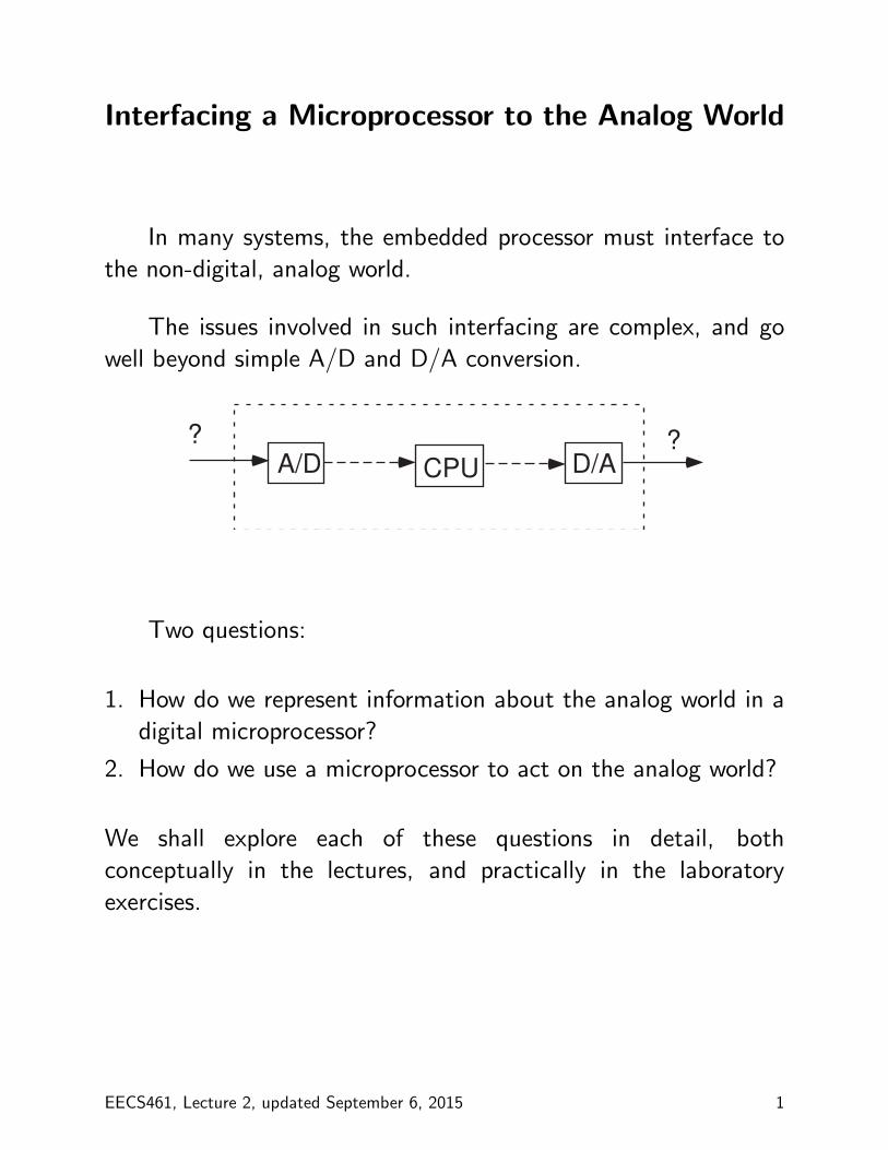
Sensors

• Used to measure physical quantities such as

- position

- velocity

- temperature

- sound

- light

• Two basic types:

- sensors that measure an (analog) physical quantity and

generate an analog signal, such as a voltage or current

A/Dsensor

physicalquantity

analogvoltage digital

* tachometer

* potentiometer

- sensors that directly generate a digital value

sensor

physicalquantity

digital

* digital camera

* position encoders


Sensor Interfacing Issues

• Shall focus on issues that involve

- loss of information

- distortion of information

• Such issues include

- quantization

- sampling

- noise

• Fundamental difference between quantization and sampling

errors:

- Quantization errors affect the precision with which we can

represent a single analog value in digital form.

- Sampling errors affect how well we can represent an entire

analog waveform (or time function) digitally.


Quantization

Digital representation of an analog number [2, 3, 6]

• Issue:

- an analog voltage can take a continuum of values

- a binary number can take only finitely many values

• Binary representation of (unsigned or signed) real number

- unipolar coding

- unipolar coding with centering

- offset binary coding

- two’s complement

• Resolution [2, 3]

- Idea: two analog numbers whose values differ by < 1/2n

may yield the same digital representation

- an n-bit A/D converter has a resolution equal to 2−n times

the input voltage range, v ∈ [0, Vmax]

- least significant bit (LSB) represents Vmax/2n


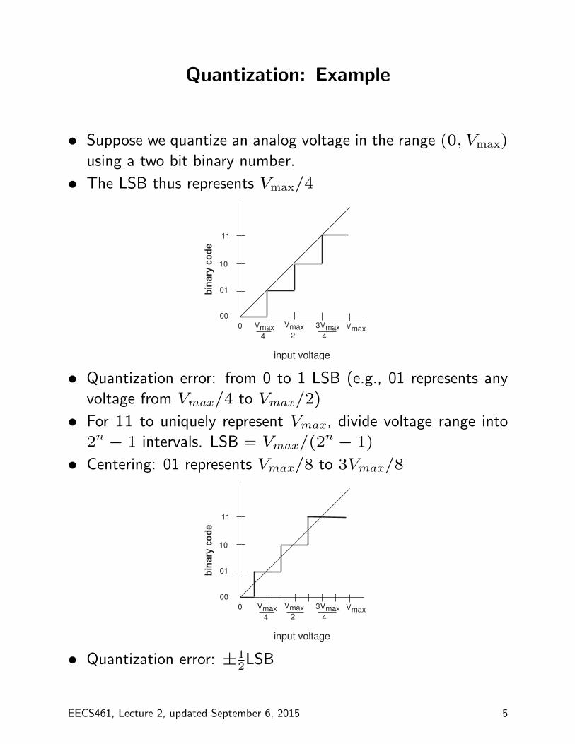
Quantization: Example

• Suppose we quantize an analog voltage in the range (0, Vmax)

using a two bit binary number.

• The LSB thus represents Vmax/4

0 Vmax3Vmax 4

Vmax 2

Vmax 4

input voltage

00

01

10

11

• Quantization error: from 0 to 1 LSB (e.g., 01 represents any

voltage from Vmax/4 to Vmax/2)

• For 11 to uniquely represent Vmax, divide voltage range into

2n − 1 intervals. LSB = Vmax/(2n − 1)

• Centering: 01 represents Vmax/8 to 3Vmax/8

0 Vmax3Vmax 4

Vmax 2

Vmax 4

input voltage

00

01

10

11

• Quantization error: ±12LSB


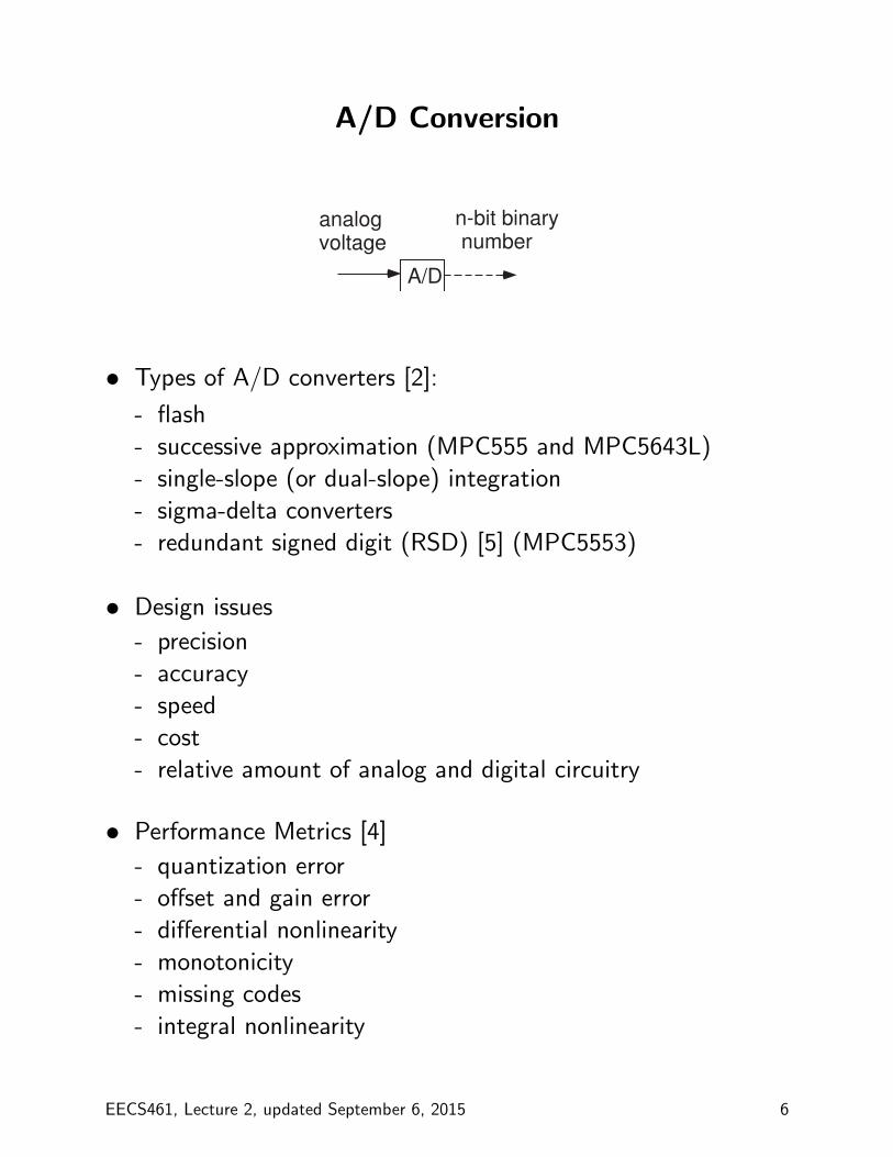
A/D Conversion

A/D

analogvoltage

n-bit binary number

• Types of A/D converters [2]:

- flash

- successive approximation (MPC555 and MPC5643L)

- single-slope (or dual-slope) integration

- sigma-delta converters

- redundant signed digit (RSD) [5] (MPC5553)

• Design issues

- precision

- accuracy

- speed

- cost

- relative amount of analog and digital circuitry

• Performance Metrics [4]

- quantization error

- offset and gain error

- differential nonlinearity

- monotonicity

- missing codes

- integral nonlinearity


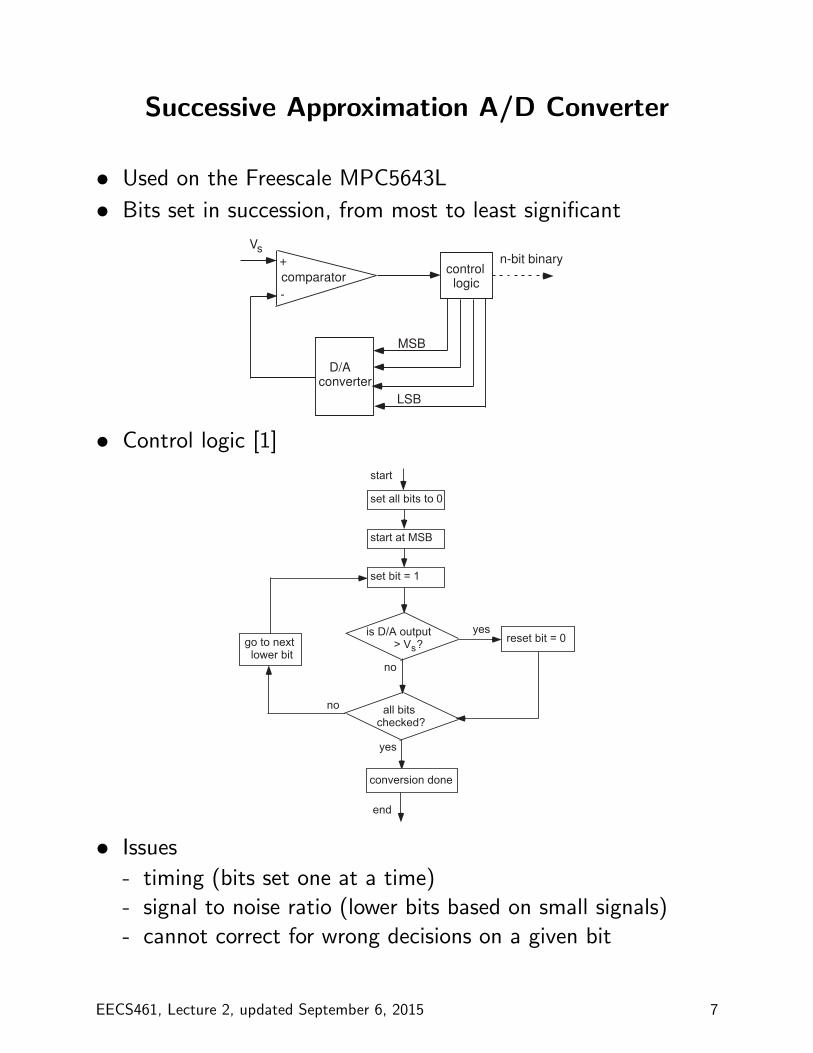
Successive Approximation A/D Converter

• Used on the Freescale MPC5643L

• Bits set in succession, from most to least significant

comparator

+

-

control logic

n-bit binary

D/Aconverter

MSB

LSB

Vs

• Control logic [1]

go to next lower bit

set all bits to 0

start at MSB

set bit = 1

is D/A output > Vs?

yesreset bit = 0

all bitschecked?

no

yes

conversion done

start

end

no

• Issues

- timing (bits set one at a time)

- signal to noise ratio (lower bits based on small signals)

- cannot correct for wrong decisions on a given bit


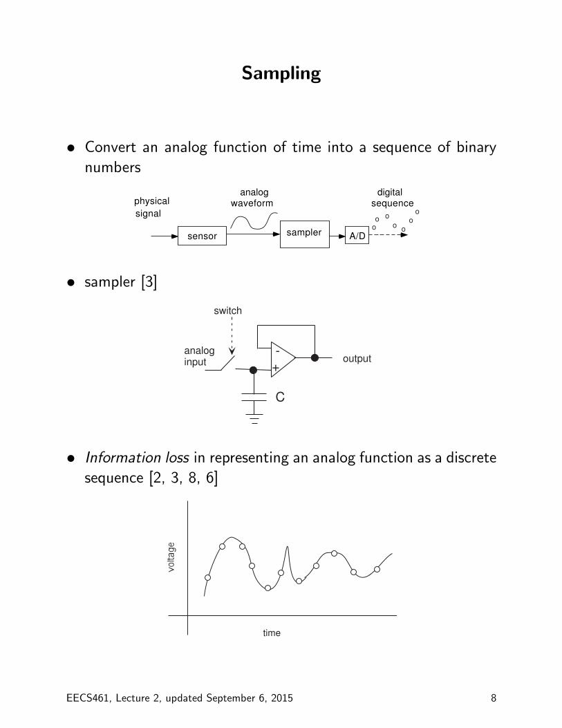
Sampling

• Convert an analog function of time into a sequence of binary

numbers

o oo o

oo

o

A/Dsensor

physical

signal

analogwaveform

digitalsequence

sampler

• sampler [3]

C

-

+

analoginput output

switch

• Information loss in representing an analog function as a discrete

sequence [2, 3, 8, 6]

time


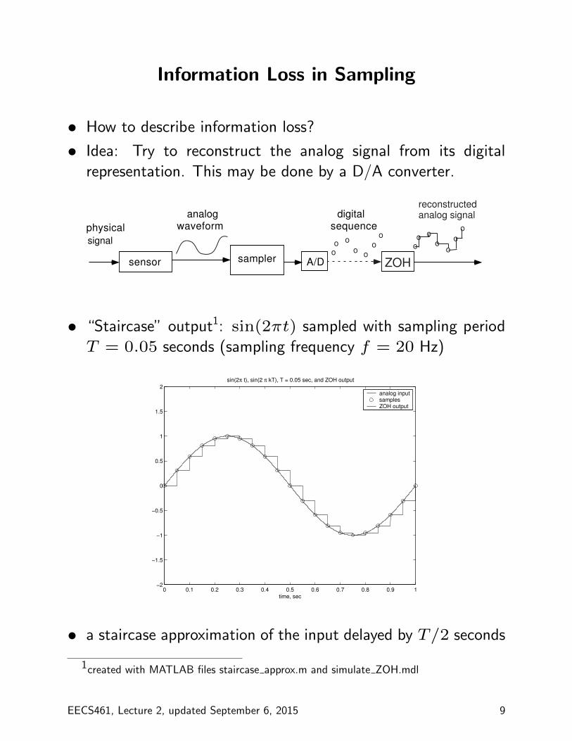
Information Loss in Sampling

• How to describe information loss?

• Idea: Try to reconstruct the analog signal from its digital

representation. This may be done by a D/A converter.

o oo o

oo

oA/Dsensor

physical

signal

analogwaveform

digitalsequence

sampler

o oo o

o

o

o

reconstructedanalog signal

ZOH

• “Staircase” output1: sin(2πt) sampled with sampling period

T = 0.05 seconds (sampling frequency f = 20 Hz)

0 0.1 0.2 0.3 0.4 0.5 0.6 0.7 0.8 0.9 1−2

−1.5

−1

−0.5

0

0.5

1

1.5

2

time, sec

sin(2π t), sin(2 π kT), T = 0.05 sec, and ZOH output

analog inputsamplesZOH output

• a staircase approximation of the input delayed by T/2 seconds

1created with MATLAB files staircase approx.m and simulate ZOH.mdl


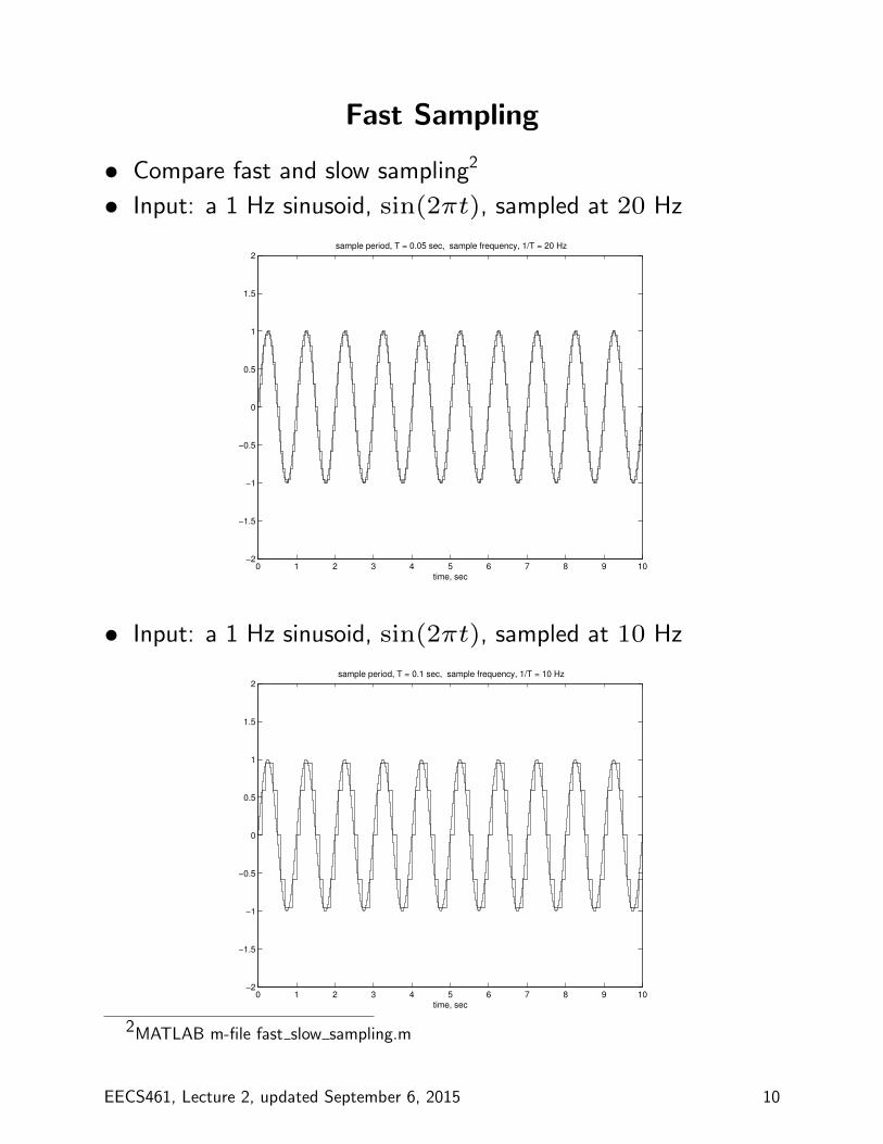
Fast Sampling

• Compare fast and slow sampling2

• Input: a 1 Hz sinusoid, sin(2πt), sampled at 20 Hz

0 1 2 3 4 5 6 7 8 9 10−2

−1.5

−1

−0.5

0

0.5

1

1.5

2sample period, T = 0.05 sec, sample frequency, 1/T = 20 Hz

time, sec


0 1 2 3 4 5 6 7 8 9 10−2

−1.5

−1

−0.5

0

0.5

1

1.5


time, sec

2MATLAB m-file fast slow sampling.m


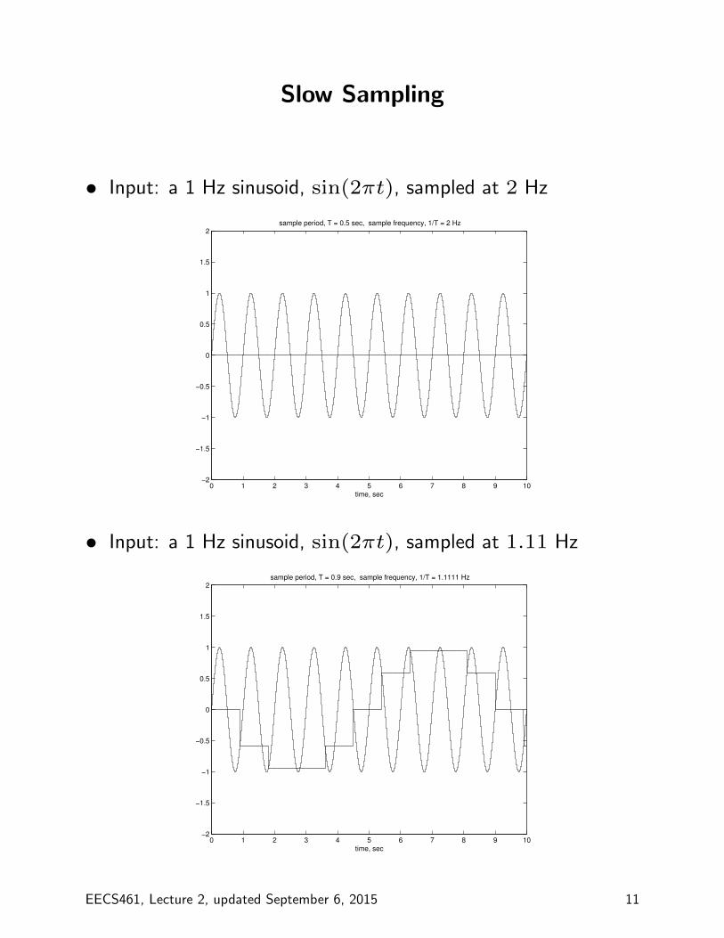
Slow Sampling


0 1 2 3 4 5 6 7 8 9 10−2

−1.5

−1

−0.5

0

0.5

1

1.5


time, sec

• Input: a 1 Hz sinusoid, sin(2πt), sampled at 1.11 Hz

0 1 2 3 4 5 6 7 8 9 10−2

−1.5

−1

−0.5

0

0.5

1

1.5

2sample period, T = 0.9 sec, sample frequency, 1/T = 1.1111 Hz

time, sec


Observations on Sampling

• If sampling period is fast with respect to period of the signal,

then the reproduced signal approximates the original signal.

- slight staircase effect

- slight time delay

• If sampling period is relatively slow, then there are the

reproduced signal may differ significantly from the original

signal.

- It may equal zero!

- It may look like a periodic signal of equal amplitude but

longer period.

• Other issues[6]

- irregular sampling interval

- synchronizing sampling with the signal


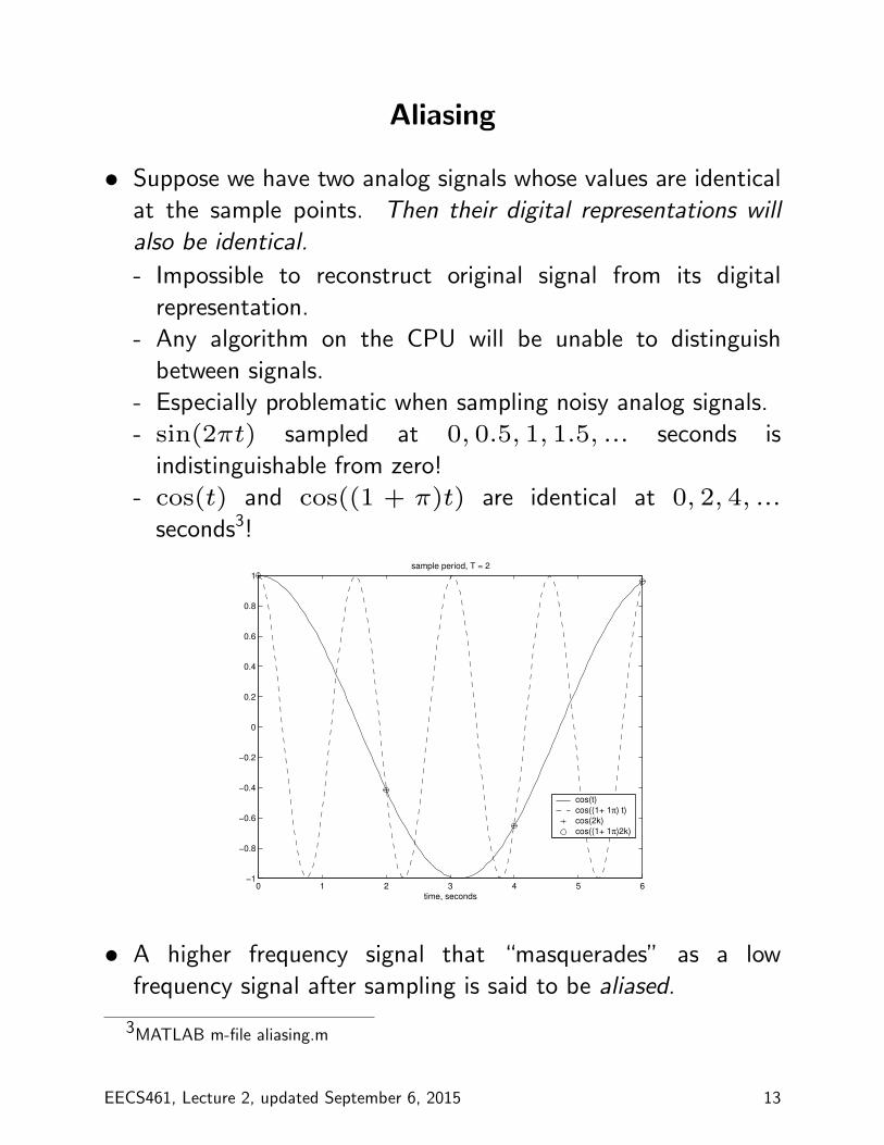
Aliasing

• Suppose we have two analog signals whose values are identical

at the sample points. Then their digital representations will

also be identical.

- Impossible to reconstruct original signal from its digital

representation.

- Any algorithm on the CPU will be unable to distinguish

between signals.

- Especially problematic when sampling noisy analog signals.

- sin(2πt) sampled at 0, 0.5, 1, 1.5, ... seconds is

indistinguishable from zero!

- cos(t) and cos((1 + π)t) are identical at 0, 2, 4, ...

seconds3!

0 1 2 3 4 5 6−1

−0.8

−0.6

−0.4

−0.2

0

0.2

0.4

0.6

0.8

1

time, seconds

sample period, T = 2

cos(t)

cos((1+ 1π) t)

cos(2k)

cos((1+ 1π)2k)

• A higher frequency signal that “masquerades” as a low

frequency signal after sampling is said to be aliased.

3MATLAB m-file aliasing.m


Effects of Aliasing

• Aliasing is a type of information distortion that results from

undersampling.

• Questions:

1. How fast must one sample an arbitrary signal to avoid

aliasing?

2. When is aliasing likely to be a problem in sensor interfacing?

3. How does one minimize the effects of aliasing?

• We shall return to these questions after an example and a

review of some ideas from signals and systems.

Example: Consider a video of a rotating wheel marked with an

arrow, and made with a camcorder at a rate of 30 frames/second

[8]...


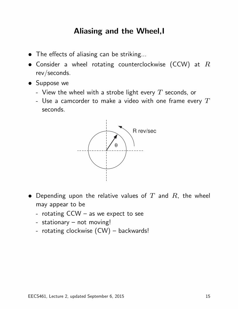
Aliasing and the Wheel,I

• The effects of aliasing can be striking...

• Consider a wheel rotating counterclockwise (CCW) at R

rev/seconds.

• Suppose we

- View the wheel with a strobe light every T seconds, or

- Use a camcorder to make a video with one frame every T

seconds.

θ

R rev/sec

• Depending upon the relative values of T and R, the wheel

may appear to be

- rotating CCW – as we expect to see

- stationary – not moving!

- rotating clockwise (CW) – backwards!


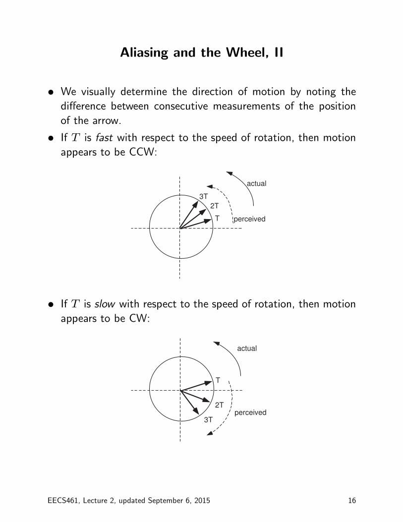
Aliasing and the Wheel, II

• We visually determine the direction of motion by noting the

difference between consecutive measurements of the position

of the arrow.

• If T is fast with respect to the speed of rotation, then motion

appears to be CCW:

T

2T

3T

actual

perceived

• If T is slow with respect to the speed of rotation, then motion

appears to be CW:

T

2T

3T

actual

perceived


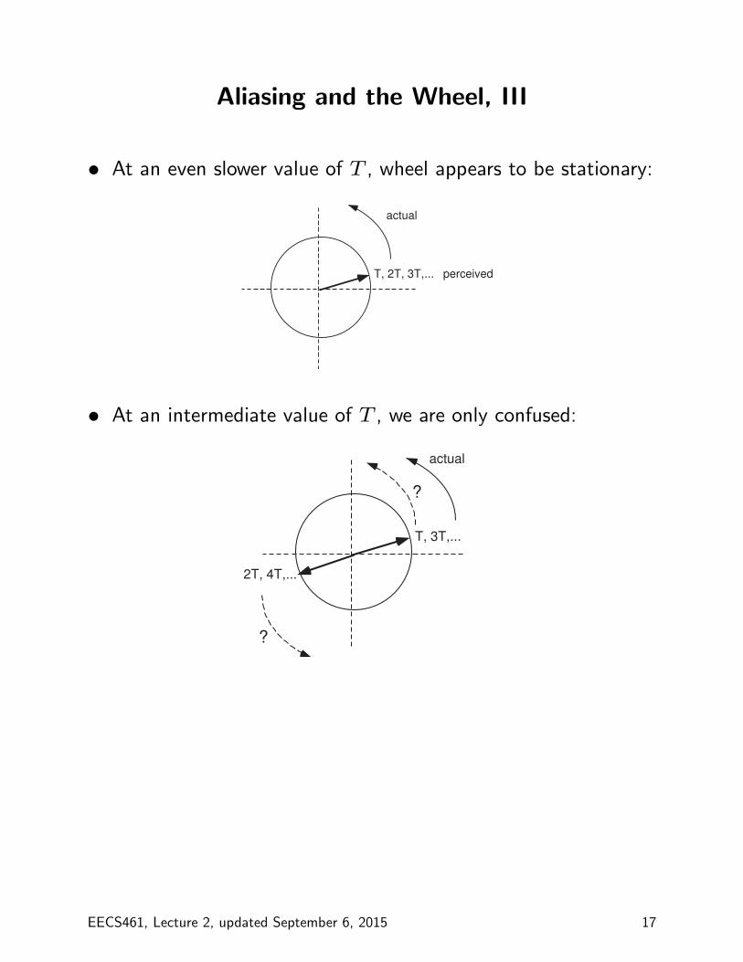
Aliasing and the Wheel, III

• At an even slower value of T , wheel appears to be stationary:

T, 2T, 3T,...

actual

perceived

• At an intermediate value of T , we are only confused:

T, 3T,...

actual

2T, 4T,...

?

?


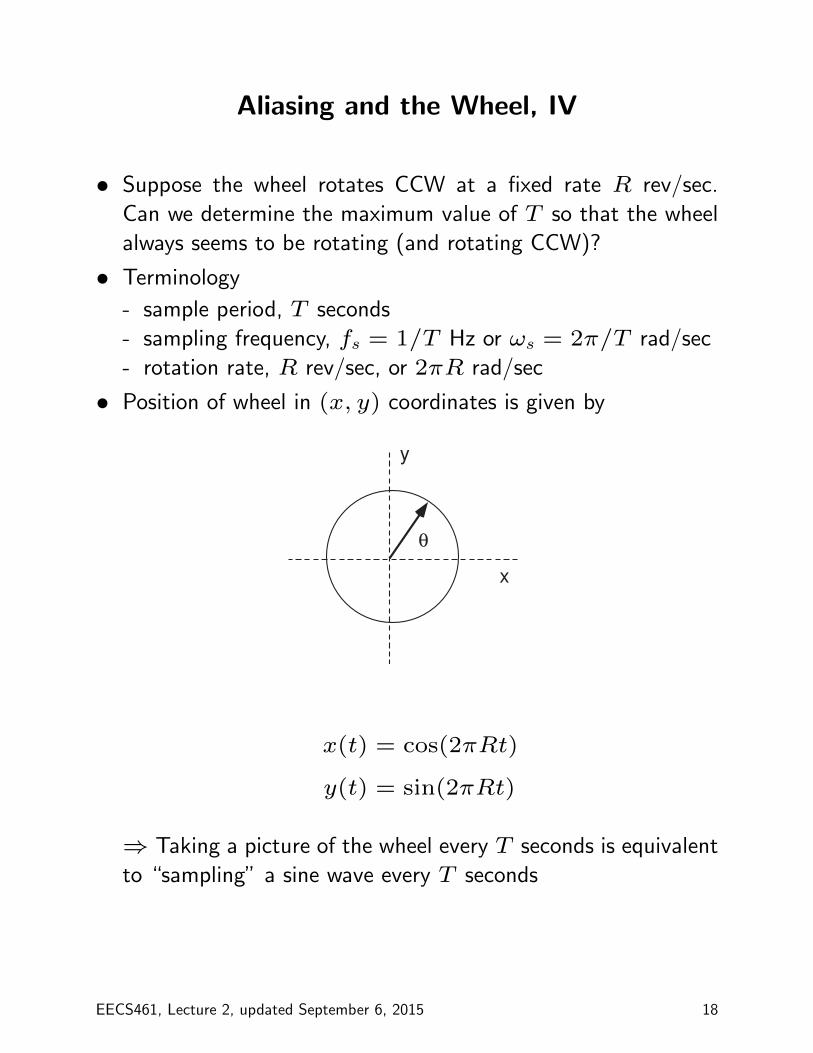
Aliasing and the Wheel, IV

• Suppose the wheel rotates CCW at a fixed rate R rev/sec.

Can we determine the maximum value of T so that the wheel

always seems to be rotating (and rotating CCW)?

• Terminology

- sample period, T seconds

- sampling frequency, fs = 1/T Hz or ωs = 2π/T rad/sec

- rotation rate, R rev/sec, or 2πR rad/sec

• Position of wheel in (x, y) coordinates is given by

θ

x

y

x(t) = cos(2πRt)

y(t) = sin(2πRt)

⇒ Taking a picture of the wheel every T seconds is equivalent

to “sampling” a sine wave every T seconds


Aliasing and the Wheel, V

• It takes 1/R seconds for the wheel to make a complete

revolution.

• Suppose that initially θ(0) = 0◦. Hence if we sample at

T = 1/R samples/second, then the position coordinates at

the sample times kT, k = 1, 2, 3... satisfy

x(kT ) = cos(2πk) = x(0) = 1

y(kT ) = sin(2πk) = y(0) = 0

⇒ the wheel looks as though it were stationary

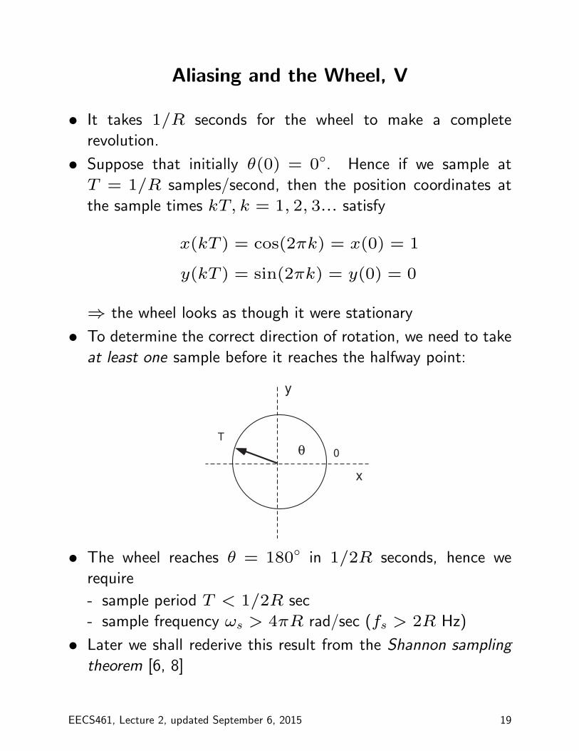
• To determine the correct direction of rotation, we need to take

at least one sample before it reaches the halfway point:

θ

x

y

T

0

• The wheel reaches θ = 180◦ in 1/2R seconds, hence we

require

- sample period T < 1/2R sec

- sample frequency ωs > 4πR rad/sec (fs > 2R Hz)

• Later we shall rederive this result from the Shannon sampling

theorem [6, 8]


Fourier Series

• Consider a periodic time signal f(t), t ≥ 0, with period T :

f(t) = f(t+ kT ), k = 0, 1, 2, . . ..

• Examples:

- sine wave

- square wave

- sawtooth wave

• Then f(t) may be expressed as a sum of (possibly infinitely

many) sines and cosines.

• Terminology

- T : period of signal

- ω0 = 2π/T : frequency in rad/sec

- f = 1/T : frequency in Hz

• Then

f(t) = a0 +

∞∑n=1

(an cos(nω0t) + bn sin(nω0t))

• More terminology

- Fourier coefficients: ai, bi- DC term: a0- fundamental: n = 1, sinusoids of frequency ω0

- harmonics: n > 1, sinusoids of frequency > ω0


Examples of Fourier Series

• Example: A sine wave with period T

f(t) = sin

(2π

Tt

)is its own Fourier series expansion

• Unit amplitude square wave with period T has Fourier

expansion

f(t) =

∞∑n=1n,odd

4

nπsin(nω0t)

where ω0 = 2π/T is the frequency of the square wave in

rad/sec (f = 1/T is the frequency in Hz)

- Fundamental: n = 1, 4π sin(ω0t)

- 1st harmonic: n = 3, 43π sin(3ω0t)

- 2nd harmonic: n = 5, 45π sin(5ω0t)


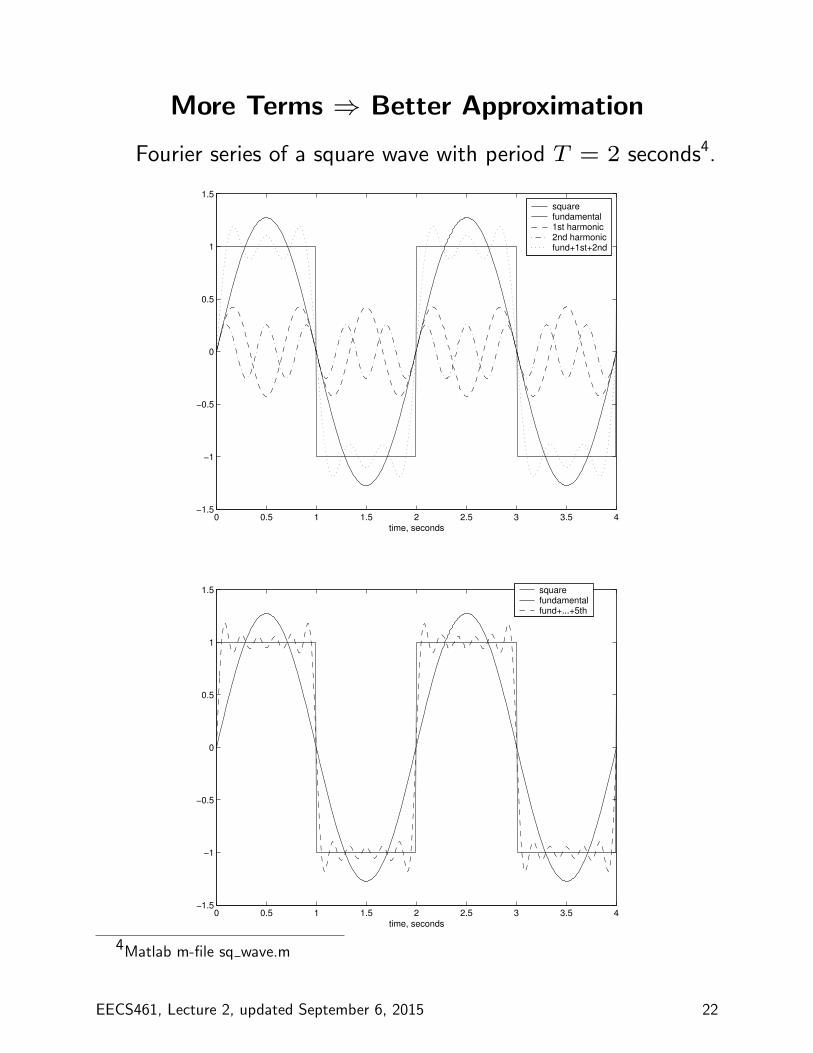
More Terms ⇒ Better Approximation

Fourier series of a square wave with period T = 2 seconds4.

0 0.5 1 1.5 2 2.5 3 3.5 4−1.5

−1

−0.5

0

0.5

1

1.5

time, seconds

square fundamental 1st harmonic2nd harmonicfund+1st+2nd

0 0.5 1 1.5 2 2.5 3 3.5 4−1.5

−1

−0.5

0

0.5

1

1.5

time, seconds

square fundamental fund+...+5th

4Matlab m-file sq wave.m


Frequency of a Signal

• Consider a periodic signal, such as a square wave, that has

“sharp corners”.

• In general, many high frequency terms are needed to construct

such “sharp corners”. In fact, any signal with relatively abrupt

changes will contain high frequencies, even if the changes are

not discontinuous.

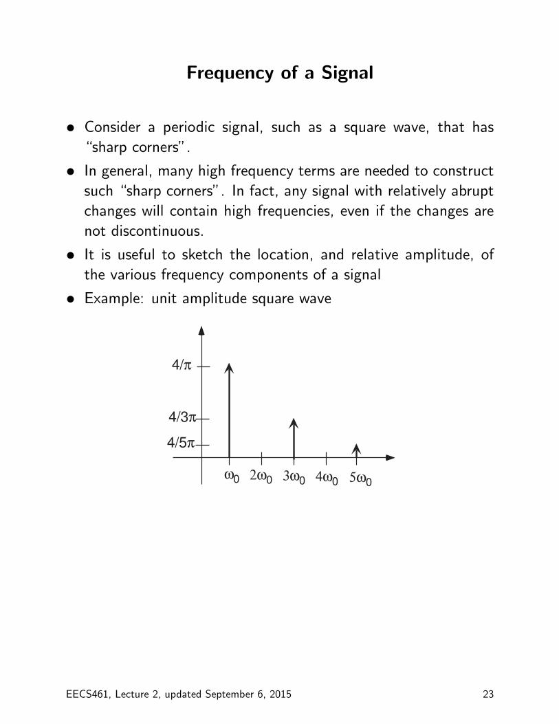
• It is useful to sketch the location, and relative amplitude, of

the various frequency components of a signal

• Example: unit amplitude square wave

ω0 2ω0

4/π

4/3π

4/5π

3ω0 4ω0 5ω0


Fourier Transform

• Most signals are not periodic. Nevertheless, it is possible to

think of “almost any” signal as the sum of sines and cosines

of all frequencies.

• Fourier transform [7]: Under certain conditions, we can write

F (ω) =

∫ ∞−∞

f(t)e−jωt

dt

=

∫ ∞−∞

f(t) cos(ωt)dt− j∫ ∞−∞

f(t) sin(ωt)dt

• Inverse Fourier transform:

f(t) =1

2π

∫ ∞−∞

F (ω)ejωtdω

• We will not need any of the details of the Fourier transform.

However, it is important to remember that time signals may

be given a frequency representation.

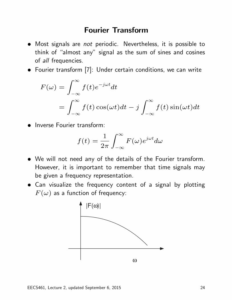
• Can visualize the frequency content of a signal by plotting

F (ω) as a function of frequency:

|F(ω)|

ω


Fourier Transform of a Periodic Signal

• Recall: delta function: δ(ω) = 0, ω 6= 0;∫∞−∞ δ(ω)dω = 1

• The Fourier transform of a sinusoid of frequency f Hz consists

of two delta functions located at frequencies ±f Hz.

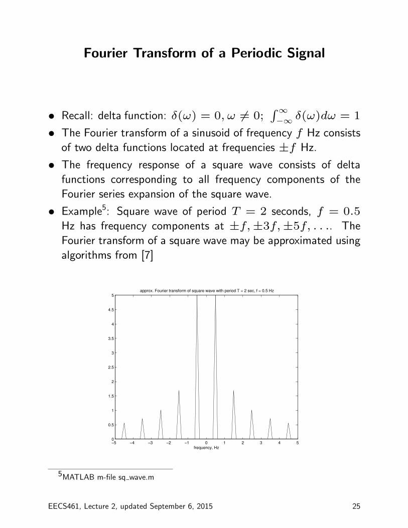
• The frequency response of a square wave consists of delta

functions corresponding to all frequency components of the

Fourier series expansion of the square wave.

• Example5: Square wave of period T = 2 seconds, f = 0.5

Hz has frequency components at ±f,±3f,±5f, . . .. The

Fourier transform of a square wave may be approximated using

algorithms from [7]

−5 −4 −3 −2 −1 0 1 2 3 4 50

0.5

1

1.5

2

2.5

3

3.5

4

4.5

5

frequency, Hz

approx. Fourier transform of square wave with period T = 2 sec, f = 0.5 Hz

5MATLAB m-file sq wave.m


Frequency Response in Embedded SystemsApplications

• Many embedded systems for control, communications, and

signal processing applications – and anything to do with audio

or video – require knowledge of frequency content of signals.

• an important class of embedded processors – DSP chips –

has a special architecture that allows rapid computation of

the frequency response of a signal using the Fast Fourier

Transform (FFT) algorithm.

• Knowledge of frequency content is needed to design the

interface electronics for an embedded system. For example,

circuits that implement lowpass filters to remove unwanted

high frequencies.

• Frequency response ideas arise in the study of sampling and

aliasing, and in the use of Pulse Width Modulation (PWM) to

drive a DC motor.


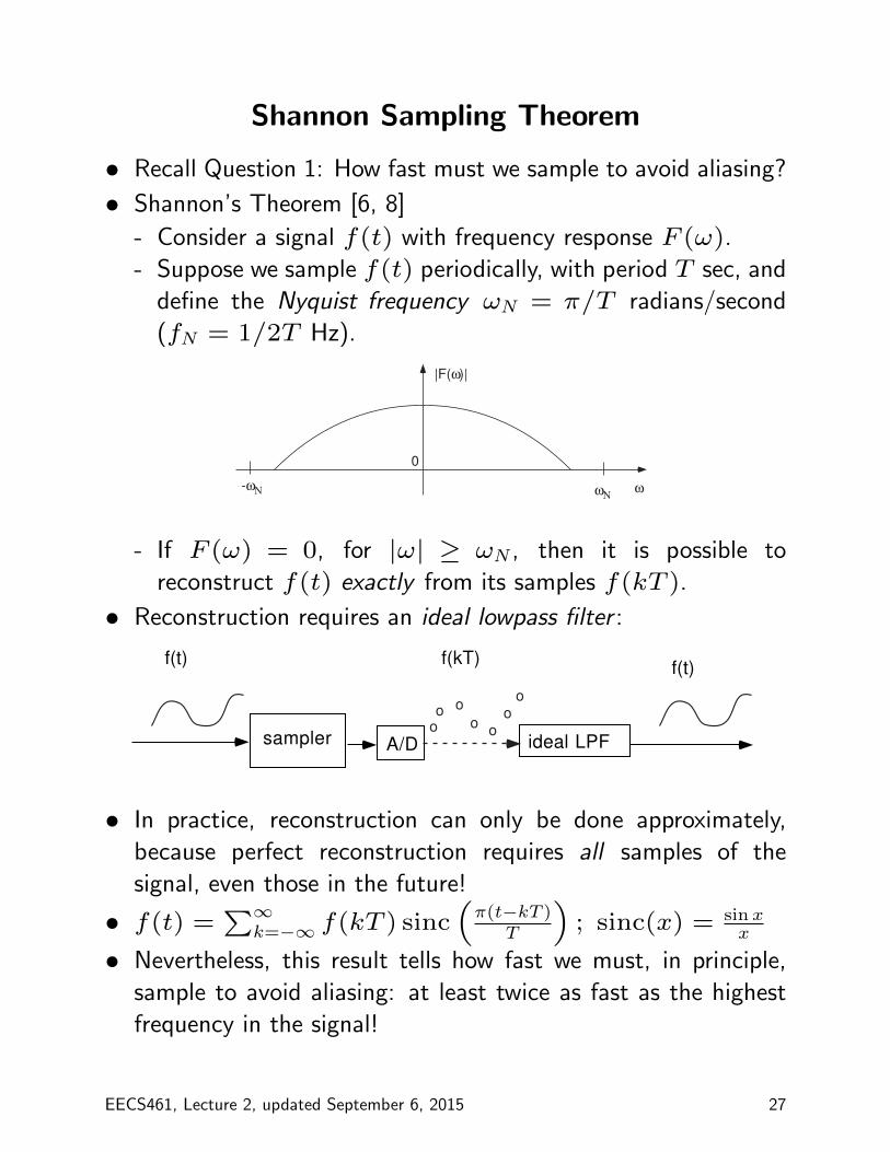
Shannon Sampling Theorem

• Recall Question 1: How fast must we sample to avoid aliasing?

• Shannon’s Theorem [6, 8]

- Consider a signal f(t) with frequency response F (ω).

- Suppose we sample f(t) periodically, with period T sec, and

define the Nyquist frequency ωN = π/T radians/second

(fN = 1/2T Hz).

|F(ω)|

ωωΝ

-ωΝ

0

- If F (ω) = 0, for |ω| ≥ ωN , then it is possible to

reconstruct f(t) exactly from its samples f(kT ).

• Reconstruction requires an ideal lowpass filter :

o oo o

oo

oA/D

f(t) f(kT)

sampler ideal LPF

f(t)

• In practice, reconstruction can only be done approximately,

because perfect reconstruction requires all samples of the

signal, even those in the future!

• f(t) =∑∞

k=−∞ f(kT ) sinc(π(t−kT )

T

); sinc(x) = sin x

x

• Nevertheless, this result tells how fast we must, in principle,

sample to avoid aliasing: at least twice as fast as the highest

frequency in the signal!


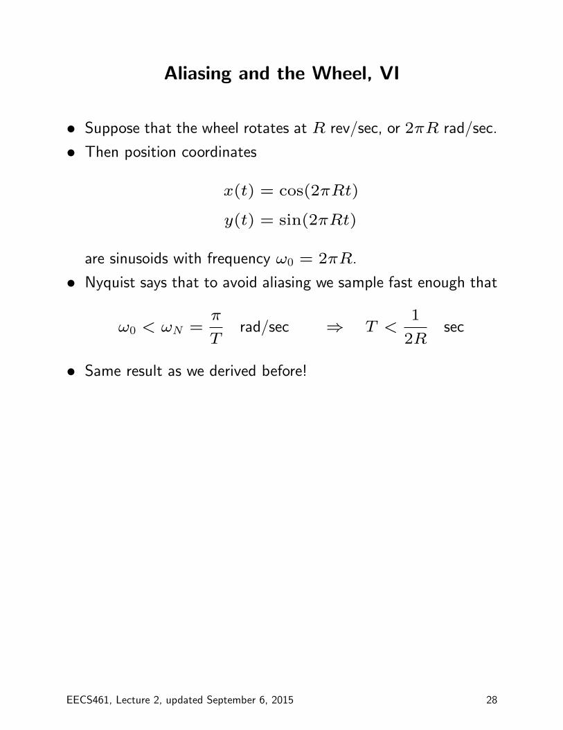
Aliasing and the Wheel, VI

• Suppose that the wheel rotates at R rev/sec, or 2πR rad/sec.

• Then position coordinates

x(t) = cos(2πRt)

y(t) = sin(2πRt)

are sinusoids with frequency ω0 = 2πR.

• Nyquist says that to avoid aliasing we sample fast enough that

ω0 < ωN =π

Trad/sec ⇒ T <

1

2Rsec

• Same result as we derived before!


Nyquist and Embedded System Applications

• A frequency analysis is done of each analog signal that must

be measured with a sensor and represented in digital form.

• Although the signals will have energy at all frequencies, usually

the “information” lies in some low frequency range, say

ω < ω0.

• If possible, set the sample period T so that the Nyquist and

sampling frequencies satisfy

ωN =π

T> ω0 ⇔ ωs =

2π

T> 2ω0

(usually, we set sampling frequency ωs > (5 − 10)ω0, twice

as fast is only the theoretical limit)


Problems with Aliasing

• When is aliasing likely to be a problem?

• Almost all signals are corrupted by noise

- 60 Hz hum

- EMI from spark ignition

-

• Often the noise is at a higher frequency than the information

contained in the signal. If the noise is at a sufficiently high

frequency, it will get “aliased” to a lower frequency, and

corrupt the signal we are trying to measure.

• How to resolve?


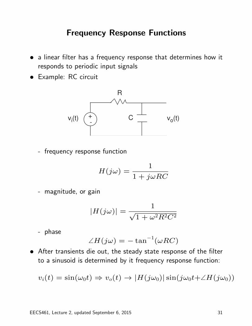
Frequency Response Functions

• a linear filter has a frequency response that determines how it

responds to periodic input signals

• Example: RC circuit

vi(t) vo(t)+-

R

C

- frequency response function

H(jω) =1

1 + jωRC

- magnitude, or gain

|H(jω)| =1

√1 + ω2R2C2

- phase

∠H(jω) = − tan−1

(ωRC)

• After transients die out, the steady state response of the filter

to a sinusoid is determined by it frequency response function:

vi(t) = sin(ω0t)⇒ vo(t)→ |H(jω0)| sin(jω0t+∠H(jω0))


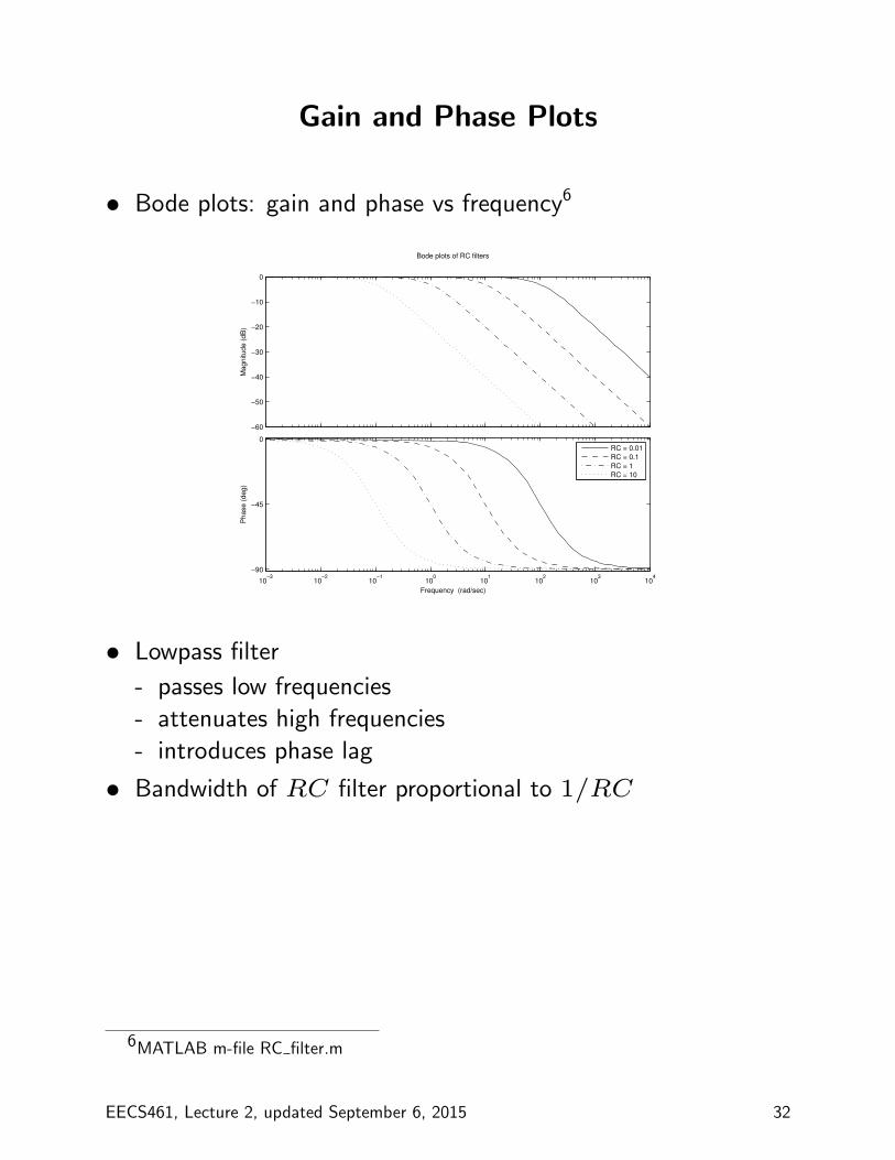
Gain and Phase Plots

• Bode plots: gain and phase vs frequency6

−60

−50

−40

−30

−20

−10

0

Ma

gn

itu

de

(d

B)

10−3

10−2

10−1

100

101

102

103

104

−90

−45

0

Ph

ase

(d

eg

)

Bode plots of RC filters

Frequency (rad/sec)

RC = 0.01

RC = 0.1

RC = 1

RC = 10

• Lowpass filter

- passes low frequencies

- attenuates high frequencies

- introduces phase lag

• Bandwidth of RC filter proportional to 1/RC

6MATLAB m-file RC filter.m


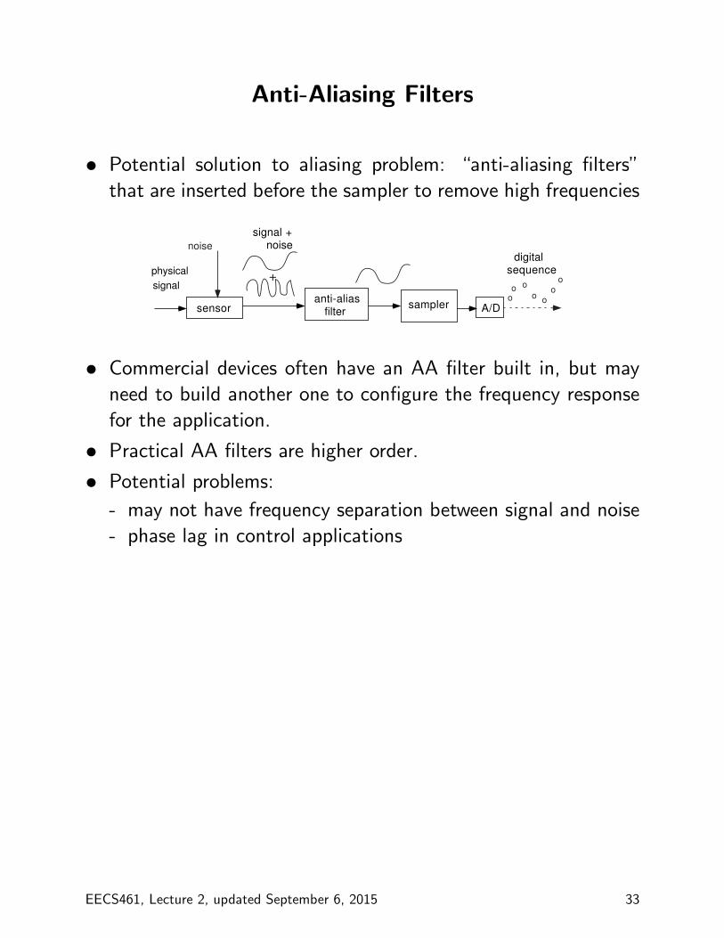
Anti-Aliasing Filters

• Potential solution to aliasing problem: “anti-aliasing filters”

that are inserted before the sampler to remove high frequencies

o oo o

oo

oA/Dsensor

physical

signal

signal + noise

digitalsequence

sampleranti-alias filter

noise

+

• Commercial devices often have an AA filter built in, but may

need to build another one to configure the frequency response

for the application.

• Practical AA filters are higher order.

• Potential problems:

- may not have frequency separation between signal and noise

- phase lag in control applications


References

[1] http://hyperphysics . phy-astr . gsu . edu /

hbase/electronic/adc . html#c3.

[2] D. Auslander and C. J. Kempf. Mechatronics: Mechanical

Systems Interfacing. Prentice-Hall, 1996.

[3] W. Bolton. Mechatronics: Electronic Control Systems in

Mechanical and Elecrical Engineering, 2nd ed. Longman,

1999.

[4] J. Feddeler and B. Lucas. ADC Definitions and Specifications.

Freescale Semiconductor, Application Note AN2438/D,

February 2003.

[5] M. Garrard and P. Ryan. Design, Accuracy, and Calibration

of Analog to Digital Converters on the MPC5500 Family.

Freescale Semiconductor, Application Note AN2989, July

2005.

[6] S. Heath. Embedded Systems Design. Newness, 1997.

[7] E. Kamen and B. Heck. Fundamentals of Signals and Systems

using MATLAB. Prentice Hall, 1997.

[8] J. H. McClellan, R. W. Schafer, and M. A. Yoder. DSP First:

A Multimedia Approach. Prentice-Hall, 1998.


Documents

A/D CPU D/A - ETH Zürich · Interfacing a Microprocessor to the Analog World In many systems, the embedded processor must interface to the non-digital, analog world. The issues involved