AD-A255 558AD-A 55 5 8 1ECHNICAL REPORT GL-92 5

STRENGTH PROPERTY ESTIMATIONf EFOR DRY, COHESIONLESS SOILS USING

THE MILITARY CONE PENETROMETER

by

Willarn E. Perkrs

Deparment o Civil --Ind Mecanica ,q ,

United States Military AcademyWest Point. New York 1099i

and

Roger W. Meier. John V. Farr

Geotechnical Laboratory

DEPARTMENT OF THE ARMYWaterways Experiment Station, Corps of Engineers

3909 Halns Ferry Road, Vicksburg, Mississippi 39180-6199

W. DTIC

May 1992

Final Report#qo-

00 - Approved For P'ubi~c Release: Distribution Is Unlriied

NII

\Prep;yCd for DEPARTMENT OF THE ARMYUS Army Corps of Engineei s

Washington, DC 20314-1000

LABORATORY r-der DA Project AT40-AM-007

92 " I 024

When this report is no longer needed return it tothe originator.

The findings in this report are not to be construed as anofficial Department of the Army position unless so

designated by other authorized documents.

The contents of this report are not to be used foradvertising, publication, or promotional purposes.Citation of trade names does not constitute anofficial endorsement or approval of the use of such

commercial products.

Form Approved

REPORT DOCUMENTATION PAGE OM No 704-01ER

UAElZ n mo, oe1 1 alel 10 - I hour per resonse. 4mIudmq the tEe n for rStatio nstructions, searchi eposting data sources.

etchia Laoaoy 99 H lserry Rfinoao.ed comnsr garigthsbrdnetmaeo2ayohr-setfti

9 $ HSOhSOR Sie 1204. AlOoRNG. VA 22202-4302. And to te Offie of m RSe e nd Budget. PS)3nook Reducion frotc (1074- 1 ). WSPON O RING . D 0IT R

1. AGENCY USE ONLY Leave blank) 12- -REPOR;T DATE 3. REPORT TYPE AND DATESNCOVERED

UMay 1992 Final reoort

4. TITLE AND SUBTITLE S. FUNDING NUMBERS

Strength Property Estimation for Dry, Cohesionless DA ProjectSoils Using the military Cone Penetrometer AT40-AM-007

6. AUTHOR(S)

William E. Perkins, Roger W. Meier, John V. Farr

7. PERFORMING ORGANIZATION NAME(S) AND ARESS(ES) .. PERFORMING ORGANIZATIONREPORT NUMBER

USAE Waterways Experiment Station Technical ReportGeotechnical Laboratory, 3909 Halls Ferry Road GL-92-5Vicksburg, MS 39180-6199

. SPONSORING MONITORING AGENCY NAME(S) AND ADRESS(E S) 10. SPONSORING MONITORINGAGENCY REPORT NUMBER

US Army Corps of EngineersWashington, DC 20314-I000

11. SUPPLEMENTARY NOTES

Available from National Technical Service,5285 Port Royal Road, Springfield, VA 22161

12a8. DISTRIBUTION / AVAILABILITY STATEMENT 12b. DISTRIBUTION CODE

Approved for public release; distribution is unlimited.

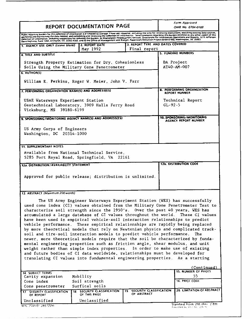
13. ABSTRACT (Maximum 200 words)

The US Army Engineer Waterways Experiment Station (WES) has successfullyused cone index (CI) values obtained from the Military Cone Penetrometer Test tocharacterize soil strength since the 1950's. Over the past 40 years, WES hasaccumulated a large database of CI values throughout the world. These CI valueshave been used in empirical vehicle-soil interaction relationships to predictvehicle performance. These empirical relationships are rapidly being replaced

by more theoretical models that rely on Newtonian physics and complicated track-soil and tire-soil interaction models to predict vehicle performance. The

newer, more theoretical models require that the soil be characterized by funda-mental engineering properties such as friction angle, shear modulus, and unit

weight rather than simple index properties. In order to make use of existing

and future bodies of C1 data worldwide, relationships must be developed for

translating CI values into fundamental engineering properties. As a starting

(Continued)14. SUBJECT TERMS 15. NUMBER OF PAGES

Cavity expansion Mobility 55

Cone index Soil strength 16. PRICE CODE

Cone penetrometer Surfical soils

17. SECURITY CLASSIFICATION 18, SECURITY CLASSIFICATION 19. SECURITY CLASSIFICATION 20. LIMITATION OF ABSTRACT

OF REPORT OF THIS PAGE OF ABSTRACT

U n c l a s s i f i e d U n c la s s i f i e d L Sta da d _f rm 298 _ _ _ _2 69

NN Standard orm 298 (50v 289)

13. ASTRACT (Concluded).

point, a simple system has been developed for estimating the unit weight, fric-tion angle, and shear modulus of dry, cohesionless soils based solely on theirUnified Soil Classification System soil classification and CI values obtained inthe field. That system is detailed in this report and a limited amount ofavailable validation data is presented.

PREFACE

The work described herein was conducted by personnel of the Department

of Civil and Mechanical Engineering, US Military Academy (USMA), West Point,

New York, and the Combat Engineering and Simulations Group (CESG), Modeling

and Methodology Branch (MMB), Mobility Systems Division (MSD), Geotechnical

Laboratory (GL), US Army Engineer Waterways Experiment Station (WES), Vicks-

burg, Mississippi. The work was sponsored by Headquarters, US Army Corps of

Engineers, and was part of DA Project AT40-AM-007, under "Inference of Classi-

cal Soil Mechanics Properties." This work was conducted between 1 June 1991

and 31 December 1991.

The analytical work was performed by and the report was written by

MAJ William E. Perkins, USMA; Mr. Roger W. Meier, CESG, GL; and Dr. John V.

Farr, CESG, GL. The study was conducted under the direct supervision of

Dr. Farr, Team Leader, under the general direction of Mr. Donald Randolph,

Chief, MMB; Mr. Newell Murphy, Jr., Chief, MSD, GL; and Dr. William F.

Marcuson III, Director, GL.

At the time of publication of this report, Director of WES was

Dr. Robert W. Whalin. Commander and Deputy Director was COL Leonard G.

Hassell, EN.

Acoession For

DTI- " AB EUnan; i. .o-:3ed Cl

C4D)it r I , : t 1on/Av:;11ibt11tv Codes*

1Dist Special

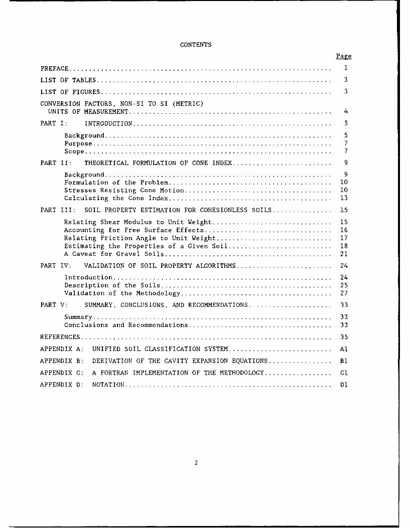
CONTENTS

Page

PREFACE..................................................................... 1

LIST OF TABLES.............................................................. 3

LIST OF FIGURES............................................................. 3

CONVERSION FACTORS, NON-SI TO SI (METRIC)

UNITS OF MEASUREMENT.................................................... 4

PART I: INTRODUCTION..................................................... 5

Background............................................................S5Purpose............................................................... 7Scope................................................................. 7

PART II: THEORETICAL FORMULATION OF CONE INDEX........................... 9

Background............................................................ 9Formulation of the Problem........................................... 10Stresses Resisting Cone Motion....................................... 10Calculating the Cone Index........................................... 13

PART III: SOIL PROPERTY ESTIMATION FOR COHESIONLESS SOILS................. 15

Relating Shear Modulus to Unit Weight................................ 15Accounting for Free Surface Effects.................................. 16Relating Friction Angle to Unit Weight............................... 17Estimating the Properties of a Given Soil............................ 18A Caveat for Gravel Soils............................................ 21

PART IV: VALIDATION OF SOIL PROPERTY ALGORITHMS.......................... 24

Introduction......................................................... 24Description of the Soils............................................. 25Validation of the Methodology........................................ 27

PART V: SUMMARY, CONCLUSIONS, AND RECOMMENDATIONS....................... 33

Summary.............................................................. 33Conclusions and Recommendations...................................... 33

REFERENCES.................................................................. 35

APPENDIX A: UNIFIED SOIL CLASSIFICATION SYSTEM............................ Al

APPENDIX B: DERIVATION OF THE CAVITY EXPANSION EQUATIONS.................. Bl

APPENDIX C: A FORTRAN IMPLEMENTATION OF THE METHODOLOGY ................... C1

APPENDIX D: NOTATION...................................................... Dl

2

LIST OF TABLES

No. Page

I Friction angle versus relative density ................................ 202 Dry unit weight versus relative density .............................. 203 Average cone profiles for the LBLG specimens ......................... 284 Soil property predictions for the LBLG specimens ..................... 305 Comparison of predicted and measured values .......................... 31

Al Detailed description of the USCS soil classes ........................ A3

LIST OF FIGURES

No. Page

1 Standard military cone penetrometer ..................................... 52 The cone penetration problem ........................................... 113 Strength correlations for granular soils ............................... 184 Effect of particle shape on void ratio ................................. 225 The MCPT in gravelly soils ............................................. 226 Strength-density relationship for Cook's Bayou sand .................. 267 Strength-density relationship for Reid-Bedford sand .................. 268 Predicted friction angle versus measured friction angle .............. 319 Predicted dry unit weight versus measured dry unit weight ............ 32

C1 Expansion of a spherical cavity ........................................ C4

3

CONVERSION FACTORS, NON-SI TO SI (METRIC)

UNITS OF MEASUREMENT

Non-SI units of measurement used in this report can be converted to SI

(metric) units as follows:

Multiply By To Obtain

degrees (angle) 0.01745329 radians

inches 2.54 centimetres

miles (US statute) 1.609347 kilometres

pounds (force) 4.448222 newtons

pounds (force) per square inch 6.894757 kilopascals

pounds (mass) per cubic foot 16.01846 kilograms per cubic metre

pounds (mass) per cubic inch 27.6799 grams per cubic centimetre

square inchc- 6.4516 square centimetres

4

STRENGTH PROPERTY ESTIMATION FOR DRY, COHESIONLESS

SOILS USING THE MILITARY CONE PENETROMETER

PART I: INTRODUCTION

Background

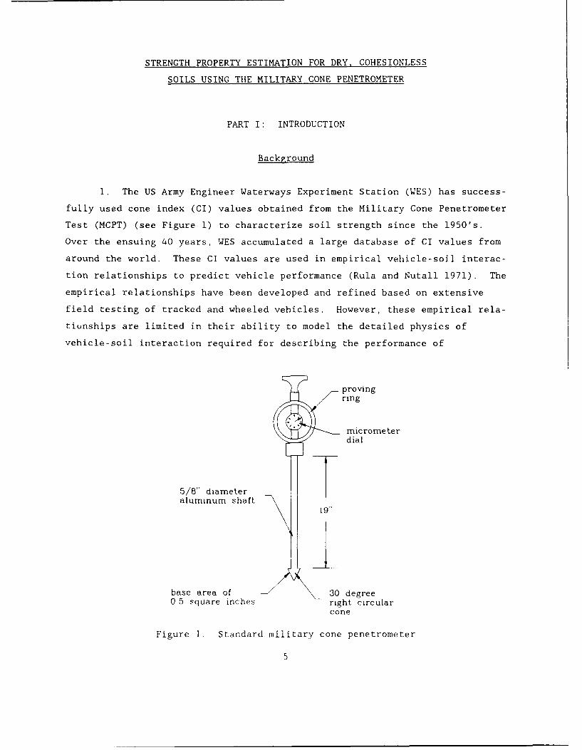
1. The US Army Engineer Waterways Experiment Station (WES) has success-

fully used cone index (CI) values obtained from the Military Cone Penetrometer

Test (MCPT) (see Figure 1) to characterize soil strength since the 1950's.

Over the ensuing 40 years, WES accumulated a large database of CI values from

around the world. These CI values are used in empirical vehicle-soil interac-

tion relationships to predict vehicle performance (Rula and Nutall 1971). The

empirical relationships have been developed and refined based on extensive

field testing of tracked and wheeled vehicles. However, these empirical rela-

tiunships are limited in their ability to model the detailed physics of

vehicle-soil interaction required for describing the performance of

provingring

micrometerdial

5/8" diameter Taluminum shaft 19"

base area of 30 degree0 5 square inches right circular

cone

Figure 1. Standard military cone penetrometer

5

maneuvering vehicles, the deformation and compaction of soils resulting from

traffic, and next-generation vehicles whose characteristics fall outside the

range of the empirical relations. To address this problem, vehicle-terrain

interaction models have become increasingly theoretical, relying on Newtonian

physics and complicated track-soil and tire-soil interaction models to predict

vehicle performance. The newer, more theoretical models require that the soil

be characterized by fundamental engineering properties such as cohesion, fric-

tion angle, shear modulus, and unit weight rather than simple index properties

such as CI.

2. The required soil properties could be obtained directly from a tri-

axial shear or direct shear test; however, tests such as those are expensive

and time-consuming and could not begin to replace the existing body of accumu-

lated CI data. The MCPT, on the other hand, is a simple, easy-to-operate,

man-portable device that provides a rapid and inexpensive means of indirectly

gaging soil strength in the field. Unfortunately, the MCPT only provides an

indirect measure of soil strength (the index property C:) rather than a direct

measure of strength and deformation. In order to make use of both the exist-

ing and future bodies of CI data worldwide, correlations with which we can

infer engineering properties from CI measurements must be developed.

3. A first attempt at inferring engineering properties from MCPT data

was undertaken by Meier and Baladi (1988). Their methodology is based on a

theoretical formulation of the CI problem using cavity expansion theory to

relate cone penetration resistance to the strength and deformation properties

uf the soil. The cavity, expansion formulation, originally derived by Rohani

and Baladi (1981), incorporates three mechanical properties (cohesion, fric-

tion angle, and shear modulus) and the total unit weight. Obviously, these

four unknown soil propertieE cannot be back-calculated directly from a single

CI measurement. To ameliorate this problem, Meier and Baladi estimate the

total unit weight and shear modulus of the soil based on its Unified Soil

Classification System (USCS) soil classification, then calculate cohesion and

friction angle from two CI measurements taken at different depths. This is

accomplished by simultaneously solving two cavity expansion equations (one at

each depth) for the two remaining unknowns.

4. The biggest drawback to the Meier and Baladi approach is that it

assumes the material is homogeneous between the two measurement depths. The

6

methodology works fairly well for granular materials because they are

reasonably homogeneous across short distances. The properties calculated for

cohesive materials, however, are not always representative of the actual in

situ soil strength because the in situ strength varies with depth due to

changes in parameters such as stress history, water content, and root density.

5. Farr (1991) eliminated the need for two CI measurements at different

depths by estimating three of the four unknowns (shear modulus, unit weight,

and friction angle) based on the USCS soil classification and solving for the

remaining unknown (cohesion) using the measured CI. The drawback to this

approach is that it does not make full use of the measured CI in cohesionless

soils. Because the cohesion is not actually an unknown--it is supposed to be

either identically zero or very nearly zero--there is no need to solve for it

using the measured CI. The measured CI is merely used to confirm that the

three estimated soil properties (friction angle, shear modulus, and unit

weight) are consistent with a soil having little or no cohesion. This

deficiency is addressed by the work presented here.

Purpose

6. This report describes the development of a simple methodology for

estimating the unit weight, friction angle, and elastic shear modulus of dry,

cohesionless soils based solely on their classification within the USCS and CI

values obtained from the field. The methodology is based on a cavity expan-

sion formulation of the cone penetration problem and empirical correlations

between the mechanical and physical properties of soils.

Scope

7. Part II presents an overview of the theoretical basis for the pro-

posed methodology. Part III details the algorithms used to estimate the

mechanical properties of soils using CI and soil classification. Part IV

presents a partial validation of the methodology which is limited by the

availability of suitable validation data. Part V contains a summary and the

conclusions.

7

8. This report also contains four appendixes. Appendix A enumerates

the soil designations used in the USCS. Appendix B presents the mathematical

derivation of the cavity expansion theory upon which the methodology is based.

Appendix C contains a listing of a FORTRAN subroutine implementing the method-

ology. Appendix D contains a listing of the notation used in this report.

8

PART II: THEORETICAL FORMULATION OF CONE INDEX

Background

9. There are many correlations between cone penetration resistance and

soil strength available for use in analyzing foundation engineering problems.

Unfortunately, very little research has been directed toward the more complex

problem of characterizing the surficial soils (i.e., to depths of 1 or 2 ft*)

that are of interest in mobility applications. Karafiath and Nowatzki (1978)

present a solution for the penetration resistance of surficial soils based on

plasticity theory. Their formulation is useful for investigating the effects

of cone geometry and penetration depth, but plasticity theory does not take

the stiffness characteristics of the soil into account. It is well known that

soil compressibility substantially affects penetration resistance (e.g., Vesic

1963; Robertson and Campanella 1983), so their approach is not particularly

well suited to investigating the influence of soil properties on penetration

resistance.

10. Rohani and Baladi (1981) used the cavity expansion theory developed

by Vesic (1972) in their formulation of cone penetration resistance. Cavity

expansion theory has been used extensively for describing cone penetration and

pile penetration resistance at depth (e.g., Baligh 1976; Vesic 1977; Baldi

et al., 1981; Greeuw et al. 1988) because it takes both the strength and the

stiffness of the soil into account. Stiffness is a particularly important

consideration in the penetration of surficial soils because the soil is not

vertically constrained and will be displaced around the cone and toward the

ground surface, thus lessening its apparent stiffness. Because it takes

stiffness into account, cavity expansion theory has been adopted as the basis

of the methodology described here.

* A table of factors for converting non-SI to SI (metric) units of measure-

ment is presented on page 4.

9

Formulation of the Problem

11. The standard military cone penetrometer consists of a proving ring,

a micrometer dial, and a 30-degree right circular cone with a base area of

0.5 in.2 connected to an aluminum staff (see Figure 1). While the cone is

advanced into the soil by hand at a more-or-less constant rate, the micrometer

dial is read, usually at 1-in. penetration intervals, to obtain the penetra-

tion resistance. The micrometer dial is calibrated to read the CI directly.

(The simplicity of the test is self-evident!)

12. The CI is actually derived from the vertical force F, acting on

the cone tip as

CI- F (1)nD2

where D is the diameter of the cone tip. This equation converts the mea-

sured force to an index value having units of stress.

13. The basic geometry of the cone tip is shown in Figure 2. The cone

tip can be characterized by its base diameter D , length L , and apex angle

2a (which are, of course, related through L tan a - D/2 ). For the standard

WES mobility cone, L = 1.48 in., D = 0.799 in., and 2a = 30 degrees. A

smaller version of the cone is also available and is often used in particu-

larly strong soils that would be difficult to penetrate by hand with the

larger cone. For the smaller cone tip, L = 0.93 in. and D = 0.5 in., thls the

base area is 0.2 in.2 instead of 0.5 in.2.

Stresses Resisting Cone Motion

14. If the tip of the cone is located at a distance Z+L from the

ground surface, the stresses acting on a finite frustrum of the cone at a

depth Z+L-n are shown in Figure 2b. In that figure, a and T are the

normal and shearing stresses, respectively, that are resisting penetration of

the cone. Integration of these stresses over the surface of the cone will

provide the magnitude of the vertical force F,

10

L

F, = f(a tana + ?) 2inr d 1 (2)0

where r - v tan a . The stresses a and r are not known a priori, so they

must be determined from the fundamental properties of the soil.

15. It has been observed in practice that the cone tends to shear the

surrounding material during penetration and the soil is observed to flow

around the cone tip and towards the surface. This indicates that the entire

shearing strength of the soil is being mobilized, so the normal and shearing

stresses in the soil can be related through some type of failure relationship.

D

Fz

77d27

a. Geometry of the problem.

T T

b Stresses on o finite frustrum of the cone

Figure 2. The cone penetration problem

11

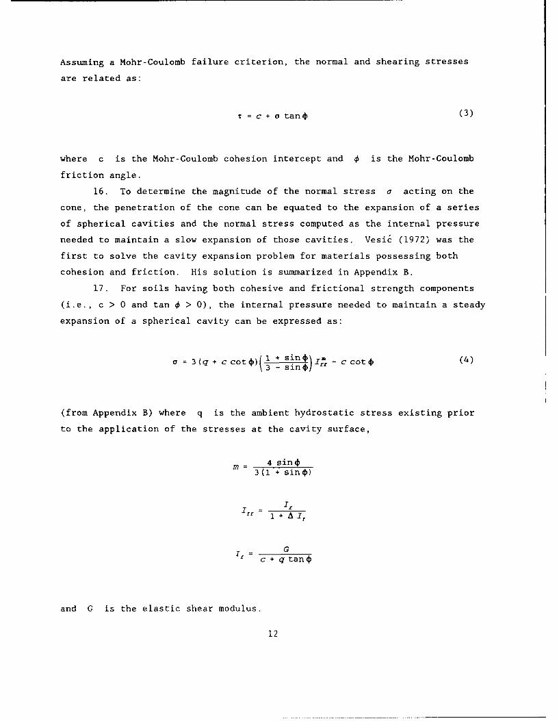
Assuming a Mohr-Coulomb failure criterion, the normal and shearing stresses

are related as:

= c + a tan4 (3)

where c is the Mohr-Coulomb cohesion intercept and 0 is the Mohr-Coulomb

friction angle.

16. To determine the magnitude of the normal stress a acting on the

cone, the penetration of the cone can be equated to the expansion of a series

of spherical cavities and the normal stress computed as the internal pressure

needed to maintain a slow expansion of those cavities. Vesic (1972) was the

first to solve the cavity expansion problem for materials possessing both

cohesion and friction. His solution is summarized in Appendix B.

17. For soils having both cohesive and frictional strength components

(i.e., c > 0 and tan 0 > 0), the internal pressure needed to maintain a steady

expansion of a spherical cavity can be expressed as:

a= 3(q+ ccoto)( 1 +Sin*)IM - c coti (4)

(from Appendix B) where q is the ambient hydrostatic stress existing prior

to the application of the stresses at the cavity surface,

m = 4 sink3(1 + sin 4)

Ir

I1=c + q tan

and G is the elastic shear modulus.

12

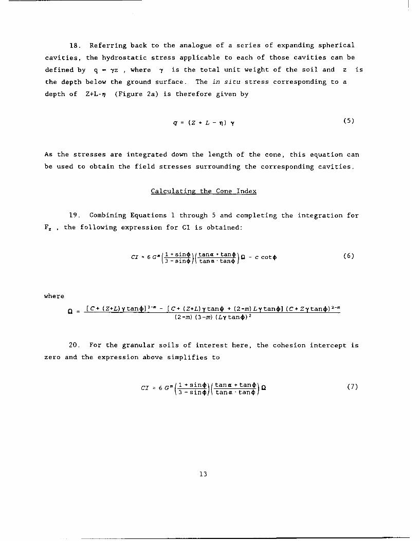
18. Referring back to the analogue of a series of expanding spherical

cavities, the hydrostatic stress applicable to each of those cavities can be

defined by q - 7z , where 7 is the total unit weight of the soil and z is

the depth below the ground surface. The in situ stress corresponding to a

depth of Z+L-n (Figure 2a) is therefore given by

q = (Z + L - TI) y (5)

As the stresses are integrated down the length of the cone, this equation can

be used to obtain the field stresses surrounding the corresponding cavities.

Calculating the Cone Index

19. Combining Equations 1 through 5 and completing the integration for

F , the following expression for CI is obtained:

CI = 6G-(l+sin)( t a n a -n+tan4)r _ c cot* (6)

where

_ (C+ (Z+L)ytan4] 3- " - [C+ (Z+L)ytan4 + (2-m)Lytan4] (C+Zytano) 2 -m

(2-m) (3-m) (Lytan0) 2

20. For the granular soils of interest here, the cohesion intercept is

zero and the expression above simplifies to

CI = 6Gm(l +sinO )tana +tan4) (7)3 -sin4) tana tant(

13

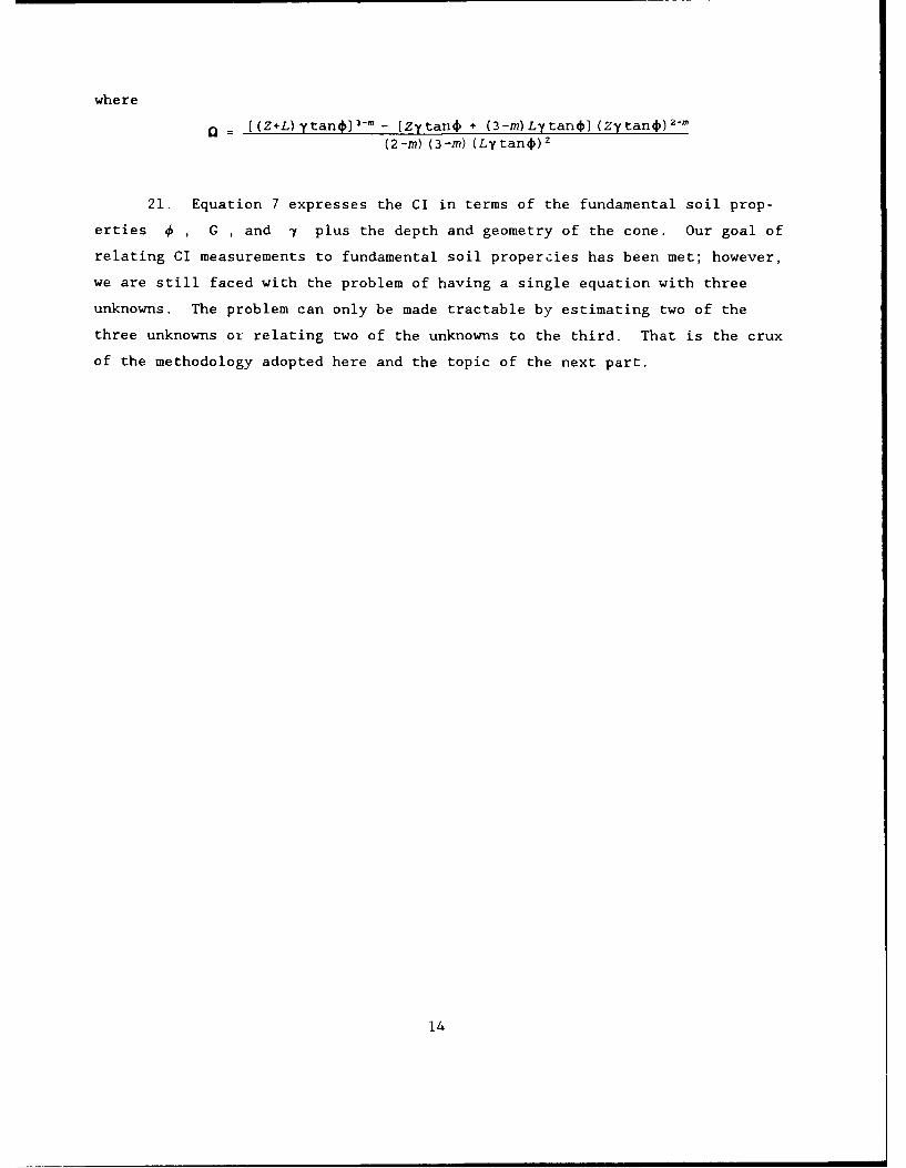
where

I [(Z+L) ytan] 3 -m - [Zytan4 + (3-m) Lytant] (ZytanO) 2 m(2--m) (3-m) (Lytano)

2

21. Equation 7 expresses the CI in terms of the fundamental soil prop-

erties 4 , G , and I plus the depth and geometry of the cone. Our goal of

relating CI measurements to fundamental soil propercies has been met; however,

we are still faced with the problem of having a single equation with three

unknowns. The problem can only be made tractable by estimating two of the

three unknowns or relating two of the unknowns to the third. That is the crux

of the methodology adopted here and the topic of the next part.

14

PART III: SOIL PROPERTY ESTIMATION FOR COHESIONLESS SOILS

Relating Shear Modulus to Unit Weight

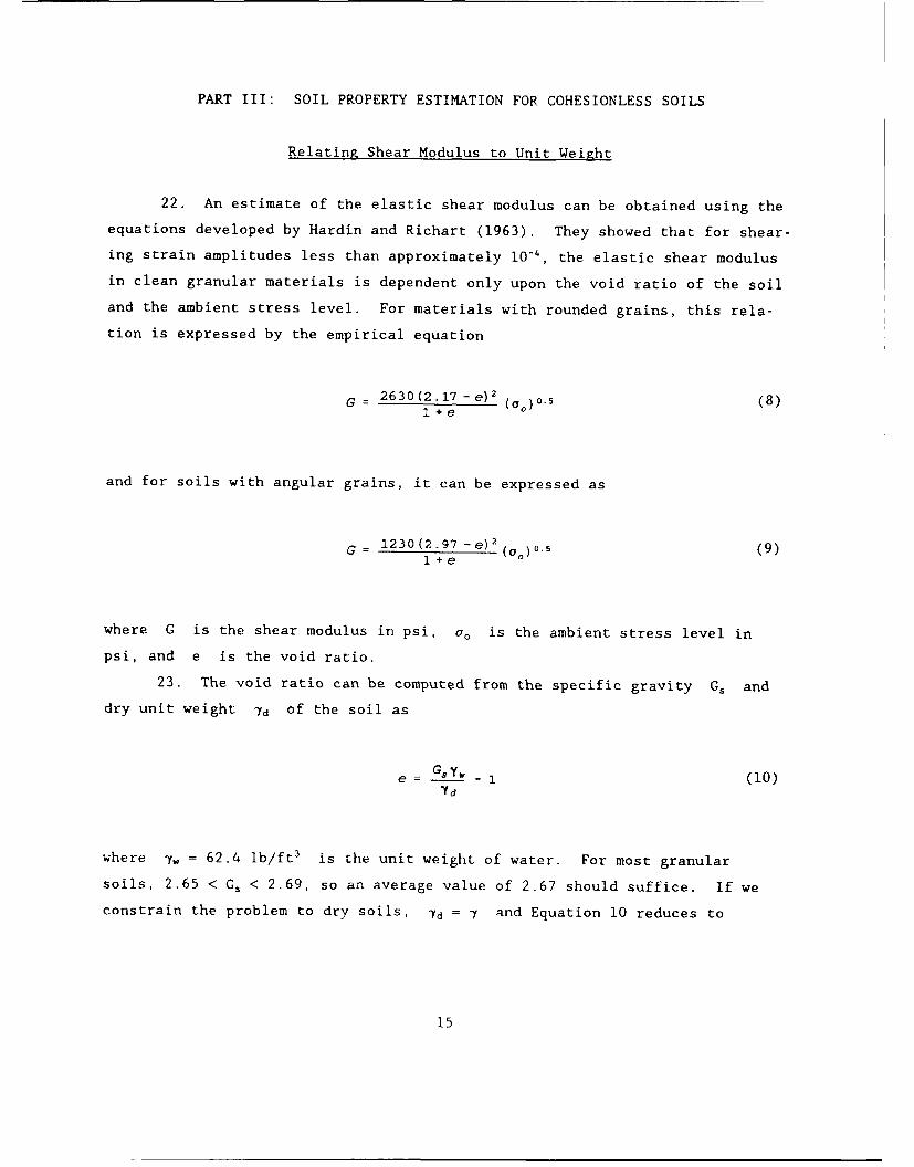
22. An estimate of the elastic shear modulus can be obtained using the

equations developed by Hardin and Richart (1963). They showed that for shear-

ing strain amplitudes less than approximately 10-', the elastic shear modulus

in clean granular materials is dependent only upon the void ratio of the soil

and the ambient stress level. For materials with rounded grains, this rela-

tion is expressed by the empirical equation

G = 2630(2.17 -e) 2 (0")0.5 (8)l+e

and for soils with angular grains, it can be expressed as

G 1230(2.97 -e) 2 (G)o.5 (9)l+e

where G is the shear modulus in psi, c. is the ambient stress level in

psi, and e is the void ratio.

23. The void ratio can be computed from the specific gravity G s and

dry unit weight Id of the soil as

=GsY 1 (10)Yd

where yw = 62.4 lb/ft 3 is the unit weight of water. For most granular

soils, 2.65 < C, < 2.69, so an average value of 2.67 should suffice. If we

constrain the problem to dry soils, 7d = 7 and Equation 10 reduces to

15

e 1 166.6-i (11)Y

where -y is expressed in lb/ft3 .

Accounting for Free Surface Effects

24. The cavity expansion equations are based upon the assumption that

the cavity expands in an unbounded medium. The process of cone penetration,

however, takes place in a medium which is bounded above by a free surface.

The existence of this free boundary allows an upward flow of the near-surface

materials in the vicinity of the cone that consequently reduces the penetra-

tion resistance of the cone. This free-surface effect is especially pro-

nounced in granular materials, but only within about 1 ft of the ground

surface. Rohani and Baladi (1981) present detailed discussions of the free

surface effect.

25. To account for the free-surface effect, Rohani and Baladi postul-

ated that the shear modulus G in Equations 6 and 7 should be replaced by an

apparent shear modulus Ga that varies with the penetration depth Z accord-

ing to the equation:

Ga =0.5[A 1 - Be-PZ G (12)1 + Be-Pz

where A , B , and 0 are constants that reflect the cone geometry and must

be evaluated expeLimentally. For the standard WES cone operating in cohesion-

less soils, A - 0.986, B = 100, and = 0.55 in. -I

26. Equation 12 assumes that G is a constant. For the surficial

soils of interest here, we can take G to be the shear modulus at the 12-in.

depth where the free surface effects become negligible. At that depth, the

hydrostatic stress co is approximately 1 psi, and Equations 8 and 9 conve-

niently reduce to

16

G 2630(2.17-e)2 (13)

i~e

and

G 1230(2.97 -e) 2 (14)

1~e

respectively. These equations uniquely relate the shear modulus to the dry

unit weight of the soil (by virtue of the void ratio being uniquely determined

by the dry unit weight). If we can also develop a correlation between fric-

tion angle and dry unit weight, we wili have a set of three equations in three

unknowns and the problem will become solvable.

Relating Friction Angle to Unit Weight

27. Many researchers have developed correlations between friction angle

and dry unit weight for cohesionless soils. The majority of those correla-

tions are, however, developed for just one or two specific soils. Conse-

quently, they are inapplicable to the problem at hand. We require a

correlation that applies to a wide range of cohesionless soil types, even if

it has less accuracy than the soil-specific correlations available in the

literature.

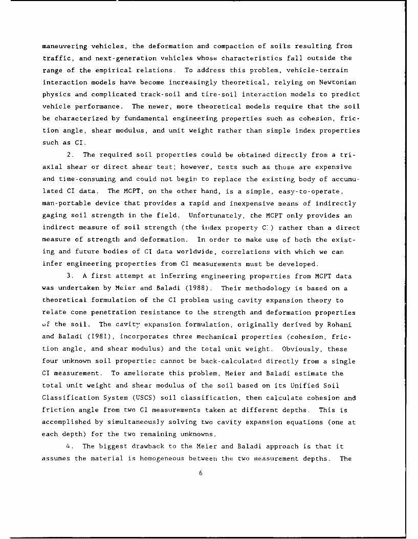
28. Figure 3 is taken from the Naval Facilities Engineering Command

Design Manual 7.01 (NAVFAC 1986). It depicts approximate correlations between

friction angle and dry unit weight for each of the cohesionless soil types in

the USCS. This is the missing piece of the puzzle. With this chart, we now

have a tractable system of three equations ( CI as a function of G , 0 , and

i'd ; G as a function of Id ; and 0 as a function of Id ) with which we

can compute the three unknown engineering properties of friction angle, shear

modulus, and unit weight using only CI measurements and the USCS

classification.

17

45 ANGLE OF INTERNAL FRICTION ..I.- -

VS DENSITY I ."-" -

(FOR COARSE GRAINED SOILS) , '

407 TYPE

nrt.- ] '- XS )r"-- '/ I ' -"- ' #'oSTAINF..D FROM

/ I o1-_ -/FALUR E EVE OPE--Z _. . . - . . APP'ROXI MATE aORREL.ATION

w 25 i I ' ' MATERIALS WITHOUT -

i { PLASTIC FINES

2o

75 80 90 0O0 110 120O 130 140) 50WOAY UNIT WEIGHT (y"D),PCF

S I I I ' I I I I I I I1.2 I.i 1.0 0.9 (18 Q75O0.7 Q6 0.5 0.5 0.5 0.4 0.3x5 0.:3 0.253 0.2 015

VOID RATIO,e

0.55 0.5 045S 0.4 0.35 0.3 0.25 0.2 0.15POROSITY,n

(G 2.68)

Figure 3. Strength correlations for granular soils

(Source: NAVFAC 1986 pg. 7.1-149)

Estimating The Properties of a Given Soil

29. Because the three equations discussed above are nonlinear, a closed

form solution for the system of equations does not exist. Instead, a numeri-

cal solution procedure will have to be adopted. A simple trial-and-error

procedure can be described as follows:

a. Assume a relative density and establish corresponding values of

qand 7Yd from the appropriate curve in Figure 3.

b. Compute a void ratio e corresponding to 7Yd usingEquation 11.

c. Compute a shear modulus C from e using either Equation 13

or Equation 14 (depending on the angularity of the grains).

18

d. Using the depth Z of the CI measurement, adjust G for free

surface effects using Equation 12.

e. Substitute 4 , 7d , Ga , and Z into Equation 7 to obtain

the theoretical value of CI.

f. If the measured CI exceeds the theoretical CI, choose a higher

relative density; otherwise, choose a lower relative density.

g. Repeat the calculations until the theoretical and measured CIvalues agree to within a suitable tolerance.

The values of 0 , Id , and G that produce a theoretical CI equal to the

measured CI are the fundamental soil properties being sought.

30. The procedure above should always converge on a solution because

all of the equations involved are monotonic. The number of iterations

required for convergence will, of course, depend on the manner in which the

iterations are performed. Since CI increases smoothly with increasing rela-

tive density (in fact, the theoretical CI is very nearly a linear function of

the logarithm of relative density), a simple binary iteration approach will

suffice.

31. Appendix C contains a FORTRAN subroutine implementing the procedure

described above. The subroutine uses binary iteration to converge on the CI

to within one percent. To prevent convergence on totally unrealistic relative

densities, the search for a solution starts at a relative density of -25 per-

cent and ends at a relative density of 150 percent. It would admittedly be

rare to find soils at relative densities significantly above 100 percent

(although it would certainly be possible to find soils at 105 to 110 percent).

This wide range of relative densities allows for soils that are more dense in

nature than they can be made using standard laboratory procedures. It also

provides some leeway for soils that do not match the NAVFAC chart exactly. If

a solution cannot be found within the range -25 percent < Dr < 150 percent,

the subroutine is exited via an alternate return.

32. Figure 3 has been implemented in the subroutine as a tabulation of

friction angle and dry unit weight values for each intersection point in the

chart. These values are given in Tables 1 and 2, respectively. Simplc liniear

interpolation within these tables is used to approximate the original curves.

In order to have a single, unique relationship for each soil type, it was

assumed a priori that SP soils will fall to the left of SM soils in the

19

Table 1. Friction angle versus relative density.

USGS 1 Relative Density (%)Soil jType 0 25 50 75 100Type

ML 25.9 28.4 31.1 33.4 36.0

SP 26.4 29.1 31.9 34.7 37.8

SM 26.9 29.7 32.9 35.9 39.1

SW 27.1 30.1 33.6 37.0 40.7

GP 27.5 30.7 34.6 38.3 42.5

GW 27.9 31.4 36.0 40.1 45.0

Table 2. Dry unit weight versus relative density.

USGS Relative Density (%)

SoilType 0 25 50 75 100

ML 79.3 83.9 88.4 92.9 97.9

SP 87.4 92.1 97.1 102.3 107.7

SM 95.0 99.6 105.0 110.0 116.0

SW 102.1 106.4 112.1 117.7 124.3

GP 109.0 114.0 120.0 126.6 133.7

GW 117.7 123.3 130.6 138.1 147.7

20

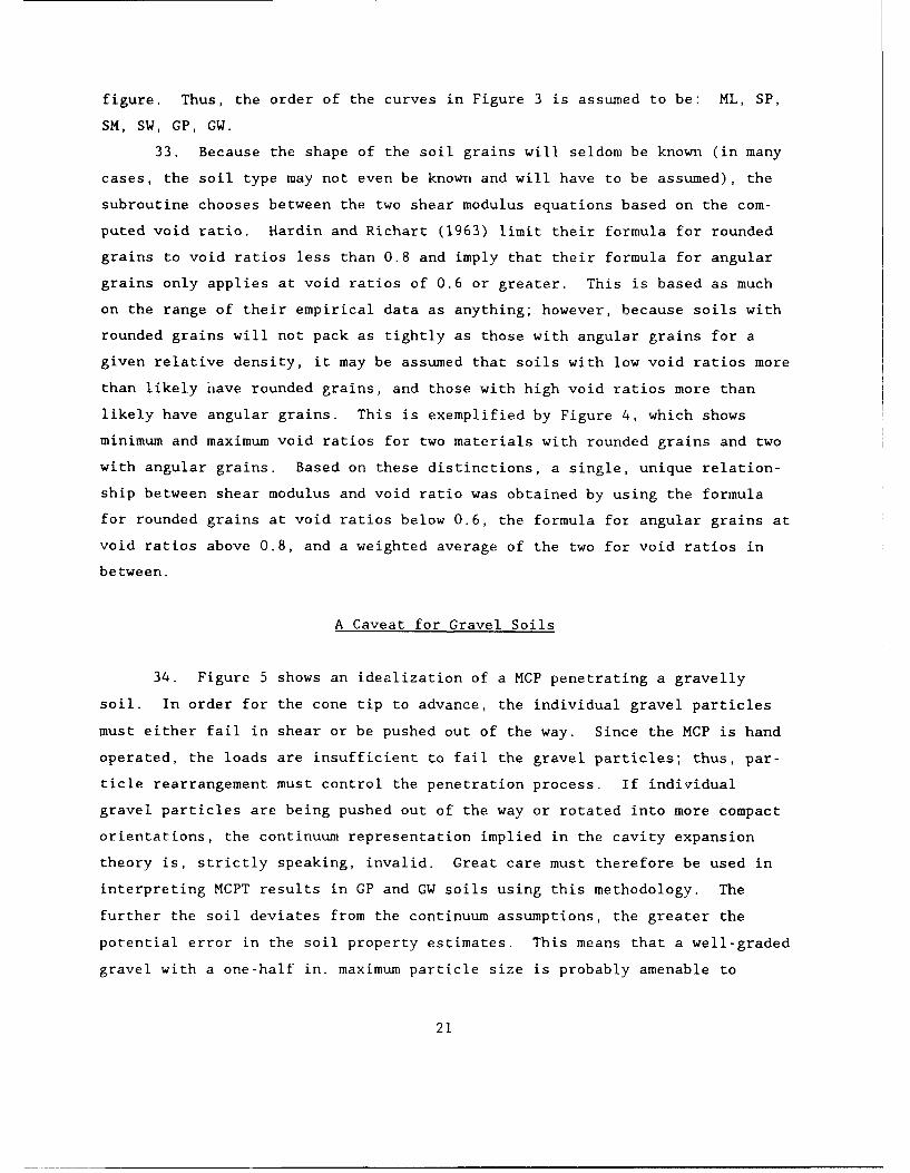
figure. Thus, the order of the curves in Figure 3 is assumed to be: ML, SP,

SM, SW, GP, GW.

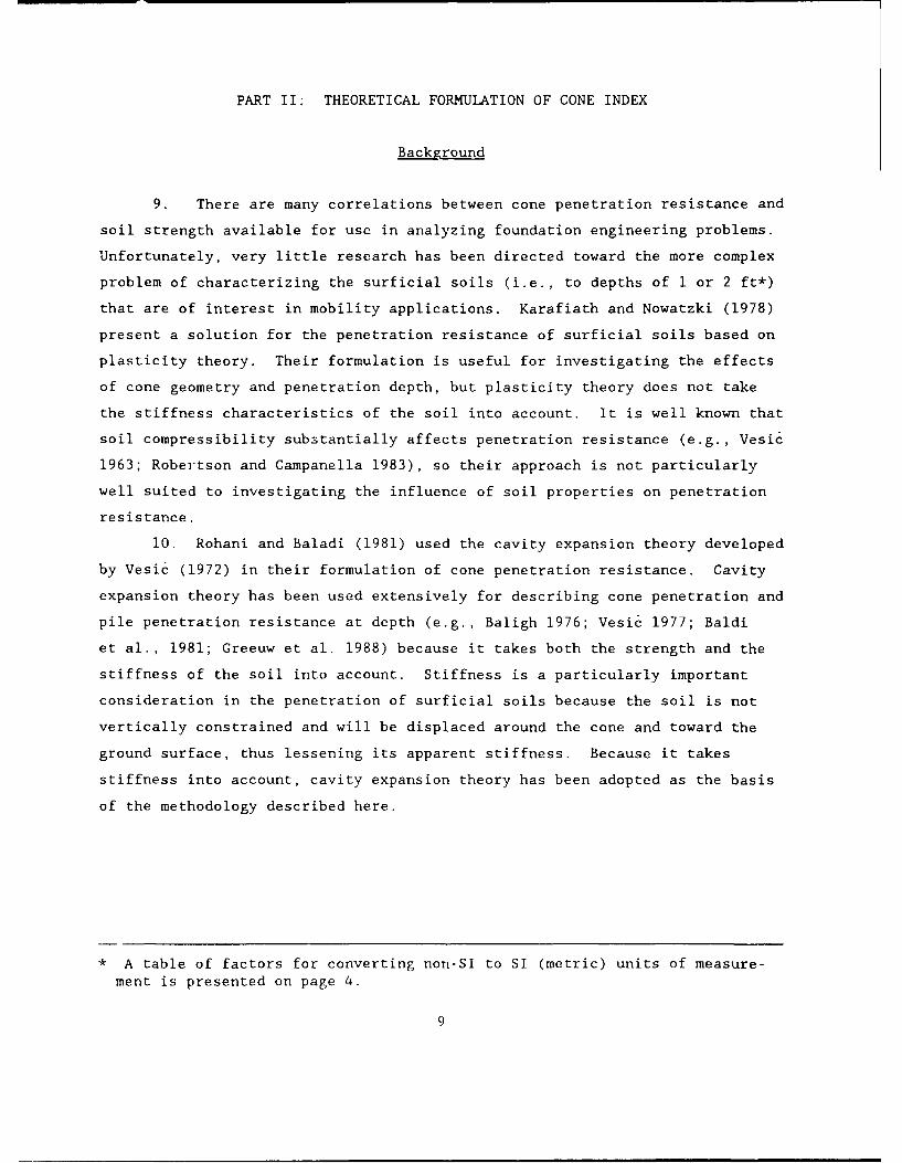
33. Because the shape of the soil grains will seldom be known (in many

cases, the soil type may not even be known and will have to be assumed), the

subroutine chooses between the two shear modulus equations based on the com-

puted void ratio. Hardin and Richart (1963) limit their formula for rounded

grains to void ratios less than 0.8 and imply that their formula for angular

grains only applies at void ratios of 0.6 or greater. This is based as much

on the range of their empirical data as anything; however, because soils with

rounded grains will not pack as tightly as those with angular grains for a

given relative density, it may be assumed that soils with low void ratios more

than likely nave rounded grains, and those with high void ratios more than

likely have angular grains. This is exemplified by Figure 4, which shows

minimum and maximum void ratios for two materials with rounded grains and two

with angular grains. Based on these distinctions, a single, unique relation-

ship between shear modulus and void ratio was obtained by using the formula

for rounded grains at void ratios below 0.6, the formula for angular grains at

void ratios above 0.8, and a weighted average of the two for void ratios in

between.

A Caveat for Gravel Soils

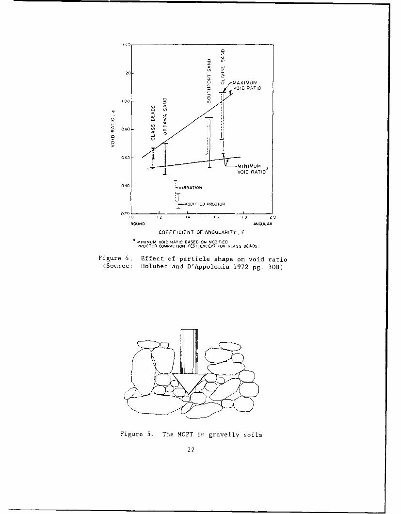
34. Figure 5 shows an idealization of a MCP penetrating a gravelly

soil. In order for the cone tip to advance, the individual gravel particles

must either fail in shear or be pushed out of the way. Since the MCP is hand

operated, the loads are insufficient to fail the gravel particles; thus, par-

ticle rearrangement must control the penetration process. If individual

gravel particles are being pushed out of the way or rotated into more compact

orientations, the continuum representation implied in the cavity expansion

theory is, strictly speaking, invalid. Great care must therefore be used in

interpreting MCPT results in GP and GW soils using this methodology. The

further the soil deviates from the continuum assumptions, the greater the

potential error in the soil property estimates. This means that a well-graded

gravel with a one-half in. maximum particle size is probably amenable to

21

4.:

z< Li

z

20>

0 -10J MAXIMUM

VOID RATIO

100

0 V)

0

VOID RATIO

040- "~~IBRATION

-iTMDFE PROCTOR

020C -1 0 12 1 4 16 8 20

ROUND ANGULAR

COEFFICIENT OF ANGULARITY, E

MINIMUM VOID RATIO BASED ON MODIFIEDPROCTOR COMPACTION TEST, EXCEPT FOR GLASS BEADS,

Figure 4. Effect of particle shape on void ratio(Source: H-olubec and D'Appolonia 1972 pg. 308)

Figure 5. The MCPT in gravelly soils

22

interpretation using this method. On the other hand, a poorly graded gravel

predominated by 2-in. particles cannot be properly analyzed.

23

PART IV: VALIDATION OF SOIL PROPERTY ALGORITHMS

Introduction

35. Ideally, validation of the algorithms presented in the preceding

chapter would be accomplished using MCP, shear strength, and density tests

conducted in situ and in close proximity to each other. The latter require-

ment is necessary to eliminate, or at least mitigate, the problems that can

arise from areal variability in the soil properties. While in situ density

tests are quite common, in situ strength tests are seldom performed. In the

dry, cohesionless soils of interest here, an alternative would be to substi-

tute empirical relations between shear strength and dry density derived from

laboratory tests on remolded soils for the in situ strength tests. This can

be done as long as the MCPT and density tests are performed in carefully com-

pacted fills devoid of horizontal layering and other density variations.

36. An extensive literature search revealed very little data that would

be suitable for validating the methodology presented in the previous chapter.

In the past, when empirical relationships based solely on CI were used for

almost all mobility modeling, there was no need to directly measure fundamen-

tal soil strength properties such as Mohr-Coulomb friction angles and cohesion

intercepts. As a result, such data were rarely collected and seldom published

(even when they were collected). Thus, the search for validation data is,

practically speaking, constrained to experimental research programs.

37. In the research arena, there is a plethora of data available from

test programs conducted in calibration chambers. Unfortunately, those test

programs almost exclusively simulated cone penetration at depths of many tr-s

of feet and stress levels far in excess of those assumed here. What little

research has been conducted in surficial soils primarily used cone penetration

resistance as the sole measure of soil strength, so there are no fundamental

strength properties to compare against.

38. The authors managed to find a limited amount of validation data by

searching through WES reports and memoranda from the 1960's when a significant

amount of experimental research was undertaken. Unfortunately, all of the

data was obtained in two remolded sands, both classified as SP under the USCS.

24

With this in mind, the remainder of this chapter presents a very limited vali-

dation of the soil property prediction methodology.

Description of the Soils

39. Two sets of unpublished data on remolded sands were obtained from a

test program conducted in the Large Blast Load Generator (LBLG) facility at

WES in the mid-1960's. The materials used in those test programs were air-dry

Cook's Bayou and Reid-Bedford Model sands.

40. Cook's Bayou sand is a uniform, fine sand taken from a borrow pit

near Cook's Bayou in the vicinity of Vicksburg, Mississippi. The material is

classified as SP according to the USCS. Its minimum and maximum dry densities

are 93.3 and 110.8, respectively. Its specific gravity is 2.65, so its maxi-

mum and minimum void ratios are 0.77 and 0.49, respectively. The grain shape

is subrounded.

41. Reid-Bedford Model sand (hereafter referred to simply as Reid-

Bedford sand) is a uniform, fine sand obtained from a borrow pit near the Big

Black River in the vicinity of Vicksburg, Mississippi. The name is derived

from the hydrologic model at WES in which it was first used. The material is

classified as SP under the USCS. Its minimum and maximum dry densities are

87.2 and 104.2 pcf, respectively. Its specific gravity is between 2.65 and

2.66, so its maximum and minimum void ratios are approximately 0.90 and 0.59,

respectively. The grain shape is on the border line between subrounded and

subangular.

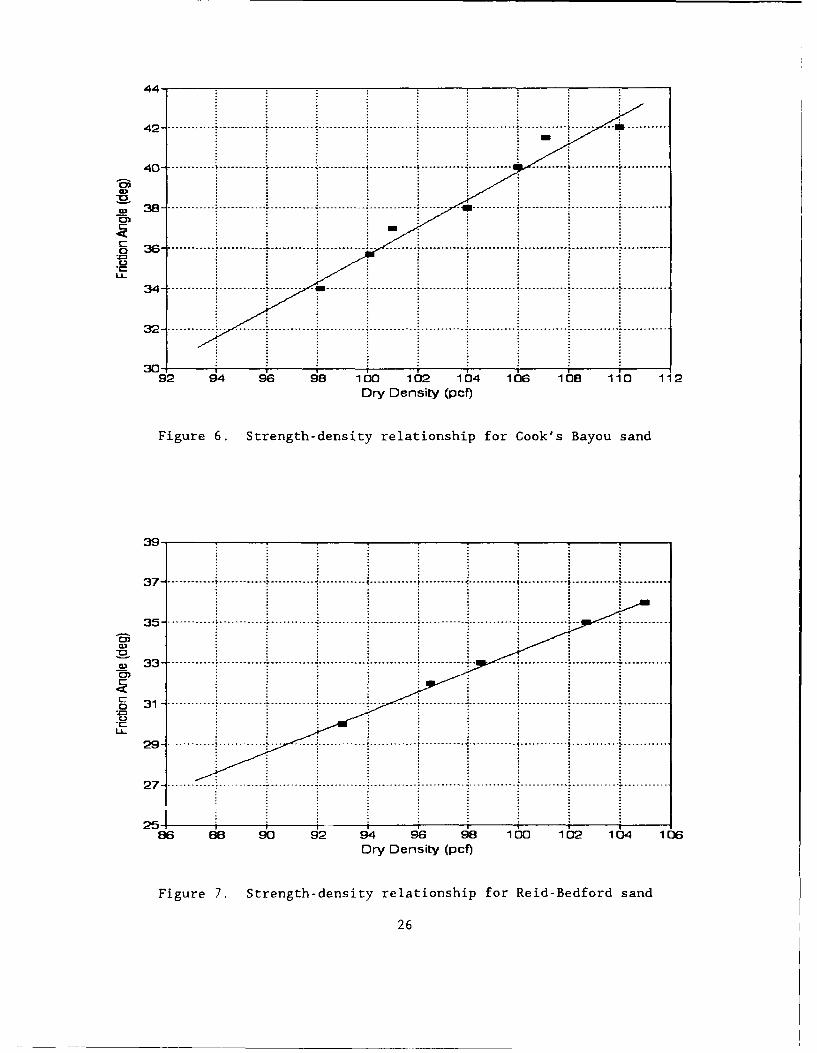
42. The strength properties of both sands have been documented in WES

reports by McNulty (1965) and Kennedy, Albritton, and Walker (1966). These

are summarized as strength-density curves in Figures 6 and 7. Also included

in those figures are least-square regression lines that are plotted over the

range of densities from minimum to maximum for each soil. The regression line

for the Cook's Bayou sand is given by

t = 0 .6 9 3 yd - 33.6 (15)

and the regression line for Reid-Bedford sand is given by

25

44.

4 2 - --- -- ------- ----- ------- ------- ----- ------- --------- - -----

4 0- ---------- - . .....4 0 ......---- --- --- --- ...- ---

3 8 -- - - - - - - - - - - -*- - - - - - - - - - - - - - - - - - - - - - - - - - - - - - - - - - - - - - - - . . .

0 38 . -............ .............. .... ............ ............ .....

34-

92 94 9 6 98 100 102 104 106 108 110 112Dry Density (pcf)

Figure 6. Strength-density relationship for Cook's Bayou sand

39r

37 . . . . . . . . . . ....... I.......-- ----- ............ ............--------- -----1 -------------------

-o_ 3 3 .-- - - - - - - - -- - . . . . . .. .. . . . .. . . . . . . . . . .. . . . . .

0 3 1 - -- ---- --- -- - ---- -------- -- ---- ------------- ------- -----

C.)

271

86 883 90 92 94 9;6 98 100 102 104 106Dry Density (pcf)

Figure 7. Strength-density relationship for Reid-Bedford sand

26

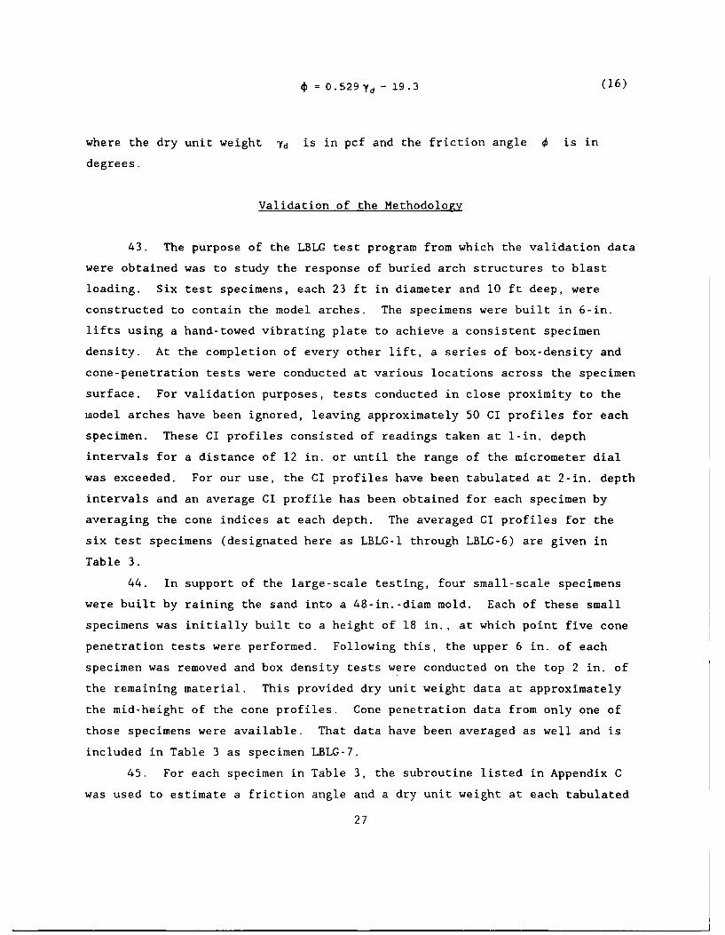
0= 0 .5 2 9 Yd - 19.3 (16)

where the dry unit weight _Yd is in pcf and the friction angle 0 is in

degrees.

Validation of the Methodology

43. The purpose of the LBLG test program from which the validation data

were obtained was to study the response of buried arch structures to blast

loading. Six test specimens, each 23 ft in diameter and 10 ft deep, were

constructed to contain the model arches. The specimens were built in 6-in.

lifts using a hand-towed vibrating plate to achieve a consistent specimen

density. At the completion of every other lift, a series of box-density and

cone-penetration tests were conducted at various locations across the specimen

surface. For validation purposes, tests conducted in close proximity to the

mnodel arches have been ignored, leaving approximately 50 CI profiles for each

specimen. These CI profiles consisted of readings taken at 1-in. depth

intervals for a distance of 12 in. or until the range of the micrometer dial

was exceeded. For our use, the CI profiles have been tabulated at 2-in. depth

intervals and an average CI profile has been obtained for each specimen by

averaging the cone indices at each depth. The averaged CI profiles for the

six test specimens (designated here as LBLG-l through LBLG-6) are given in

Table 3.

44. In support of the large-scale testing, four small-scale specimens

were built by raining the sand into a 48-in.-diam mold. Each of these small

specimens was initially built to a height of 18 in., at which point five cone

penetration tests were performed. Following this, the upper 6 in. of each

specimen was removed and box density tests were conducted on the top 2 in. of

the remaining material. This provided dry unit weight data at approximately

the mid-height of the cone profiles. Cone penetration data from only one of

those specimens were available. That data have been averaged as well and is

included in Table 3 as specimen LBLG-7.

45. For each specimen in Table 3, the subroutine listed in Appendix C

was used to estimate a friction angle and a dry unit weight at each tabulated

27

Table 3. Average cone profiles for the LBLG test specimens.

Mean Dry Cone Cone MeanSpecimen Soil Unit Weight Diameter Depth Cone IndexNumber Type (pcf) (in.) (in.) (psi)

LBLG-I Cook's Bayou 101.4 0.8 2 404 916 1828 275

LBLG-2 Cook's Bayou 107.0 0.5 2 584 1436 2828 43910 521

LBLG-3 Feid-Bedford 100.5 0.5 2 274 60

6 1078 201

10 28012 383

LBLG-4 Cook's Bayou 107.4 0.5 2 564 1336 2538 39710 533

LBLG-5 Cook's Bayou 101.7 0.5 2 364 696 1248 22610 289

12 363

LBLG-6 Reid-Bedford 106.5 0.5 2 684 1546 2908 49310 611

LBLG-7 Cook's Bayou 107.8 0.5 2 354 866 1528 22510 29012 360

28

depth. The soil type and CI data input to the subroutine and the friction

angle and dry unit weight estimates output from it are presented in Table 4.

For each test specimen, a comparison between the soil properties measured in

the LBLG (actually, the dry unit weights measured in the LBLG and friction

angles computed from those data using Equations 15 and 16) and the average of

the predicted soil properties are given in Table 5.

46. To better illustrate the amount of agreement, the predicted fric-

tion angles are plotted against the measured friction angles in Figure 8 and

the predicted dry unit weights are plotted against the measured dry unit

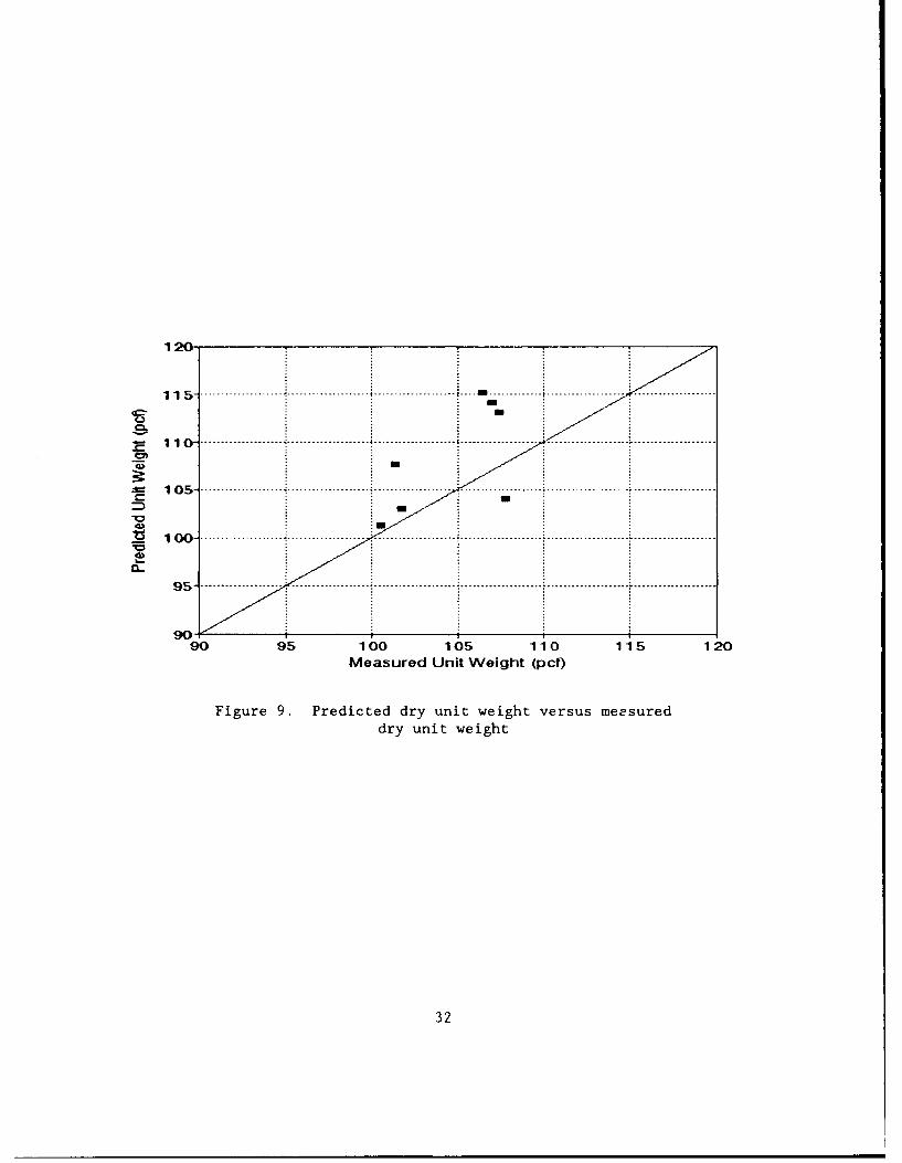
weights in Figure 9. Both figures show very good agreement between the pre-

dicted and the measured values. There seems to be a slight tendency towards

overprediction, especially for the unit weights, but the degree of overpredic-

tion is slight.

47. The data presented here by no means constitute complete validation

of the model; however, it does show the potential predictive capabilities of

the methodology. Based of these results, continued work, in the form of fur-

ther validation and refinement of the model, is definitely warranted.

29

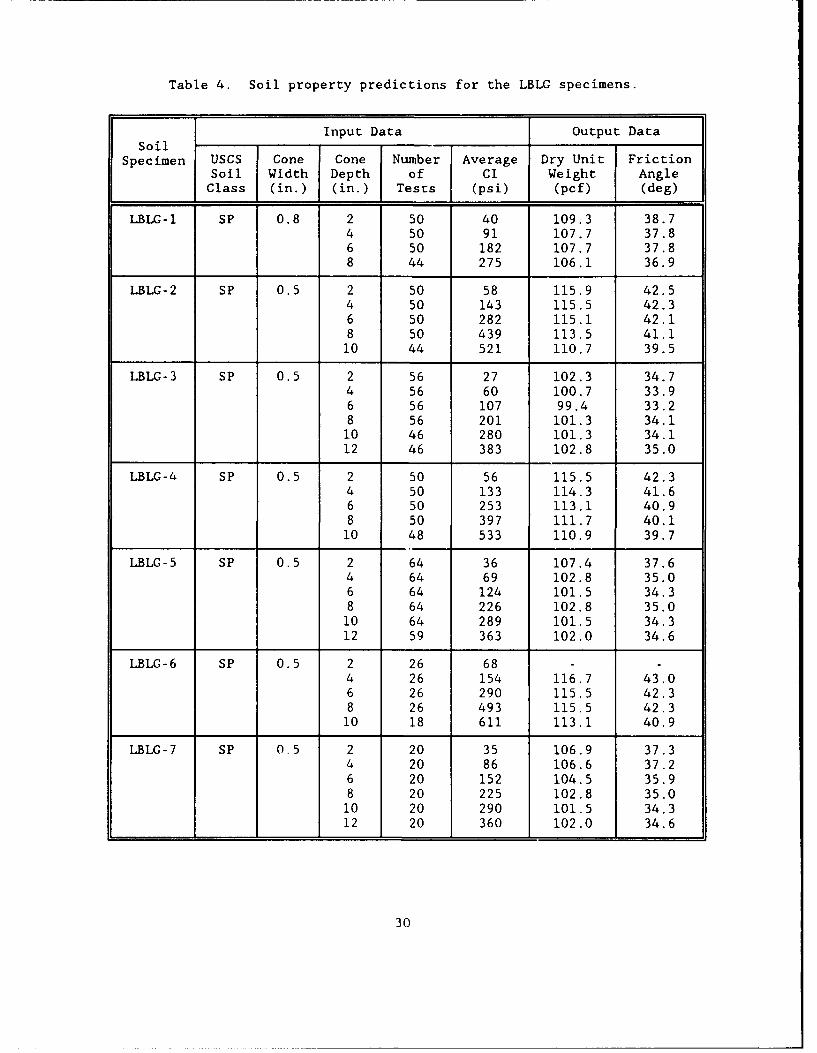
Table 4. Soil property predictions for the LBLG specimens.

Input Data Output DataSoil

Specimen USCS Cone Cone Number Average Dry Unit FrictionSoil Width Depth of CI Weight AngleClass (in.) (in.) Tests (psi) (pcf) (deg)

LBLG-1 SP 0.8 2 50 40 109.3 38.74 50 91 107.7 37.86 50 182 107.7 37.88 44 275 106.1 36.9

LBLG-2 SP 0.5 2 50 58 115.9 42.54 50 143 115.5 42.36 50 282 115.1 42.18 50 439 113.5 41.110 44 521 110.7 39.5

LBLG-3 SP 0.5 2 56 27 102.3 34.74 56 60 100.7 33.96 56 107 99.4 33.28 56 201 101.3 34.110 46 280 101.3 34.112 46 383 102.8 35.0

LBLG-4 SP 0.5 2 50 56 115.5 42.34 50 133 114.3 41.66 50 253 113.1 40.98 50 397 111.7 40.110 48 533 110.9 39.7

LBLG-5 SP 0.5 2 64 36 107.4 37.64 64 69 102.8 35.06 64 124 101.5 34.38 64 226 102.8 35.0

10 64 289 101.5 34.312 59 363 102.0 34.6

LBLG-6 SP 0.5 2 26 68 -

4 26 154 116.7 43.06 26 290 115.5 42.38 26 493 115.5 42.310 18 611 113.1 40.9

LBLG-7 SP 0.5 2 20 35 106.9 37.34 20 86 106.6 37.26 20 152 104.5 35.98 20 225 102.8 35.010 20 290 101.5 34.312 20 360 102.0 34.6

30

Table 5. Comparison of predicted and measured values.

Dry Unit Weight (pcf) Friction Angle (deg)Soil Soil

Specimen Type Measured Predicted Measured Predicted

LBLG-I Cook's Bayou 101.4 107.7 36.7 37.8

LBLG-2 Cook's Bayou 107.0 114.1 40.6 41.5

LBLG-3 Reid-Bedford 100.5 101.3 33.8 34.2

LBLG-4 Cook's Bayou 107.4 113.1 40.8 40.9

LBLG-5 Cook's Bayou 101.7 103.0 34.5 35.1

LBLG-6 Reid-Bedford 106.5 115.2 40.2 42.1

LBLG-7 Cook's Bayou 107.8 104.1 37.7 35.7

45

4 2 .................................................. ............................... ............ ........................

---39..........

30

30 t t

30 T3 36 39 42 45Measured Friction Angle (deg)

Figure 8. Predicted friction angle versus measuredfriction angle

31

1 20

1 1 5 --------------- --- - ---- ------------ .........

.0

- 1 0 ---------- ---------- --------- ------------ -------- ----------

90-

Measured Unit Weight (pcf)

Figure 9. Predicted dry unit weight versus measureddry unit weight

32

PART V: SUMMARY, CONCLUSIONS, AND RECOMMENDATIONS

Summary

48. A methodology has been presented for estimating the fundamental

engineering properties of cohesionless soils from data collected with the MCP.

The theoretical approach couples static force equilibrium with cavity expan-

sion theory to model the response of the soil to penetration by a cone tip.

The mathematical description of the cone penetration process is augmented by

several empirical relationships that serve to reduce the number of unknowns

and make the problem tractable. Limited validation using unpublished data

collected in two SP soils shows that the technique can provide reasonable

estimates of total unit weight and Mohr-Coulomb friction angle. This partial

validation suggests that the methodology warrants further development.

Conclusion" and Recommendations

49. Additional va'.1 , -ion data are needed before this method can be

used without reservati-,n. Continued literature searches and additional labo-

ratory and field e>perimentation are needed to further validate and refine the

methodology. In order to be usable, validation data must include in situ mea-

surements of unit weight, shear strength, shear stiffness, and cone penetra-

tion resistance--all taken in close proximity to one another.

50. Future research should be directed towards refining thz existing

methodology for cohesionless soils and extending the theory to cohesive soils.

It is hoped that, eventually, a system can be devised that is applicable in

all .oil types. One approach would be to collect several methodologies such

as the one described here and embed them within a knowledge-based-system

(KBS). A KBS (which includes, but is not limited to, so-called "expert sys-

tfms") is a computer program that combines knowledge about a specific domain

Lnd reasoning abilities to arrive at conclusions. In the domain of soil-

property estimation, a KBS might combine cone penetration and soil description

data supplied by the user with a collection of theoretical and empirical

models to arrive at estimates of the soil properties. The KBS would choose

the appropriate model(s), infer or ask for any missing data, and sort out the

33

often conflicting answers that the models produce. The research described

here is a first step towards producing such a system.

34

REFERENCES

Baldi, G., Bellotti, R., Ghionna, V., Jamiolkowski, M., and Pasqualini, E.1981. "Cone Resistance of a Dry Medium Sand," Proceedings, 10th InternationalConference on Soil Mechanics and Foundation Engineering, Stockholm, Vol 2,pp 427-432.

Baligh, M. M. 1976. "Cavity Expansion in Sand with Curved Envelopes," Jour-nal of the Geotechnical Engineering Division, ASCE, Vol 102, No. GTlI,pp 1131-1146.

Farr, J. V. 1991. "Shear Strength Properties From Cone Index Tests," Pro-ceedings, 5th European Conference of the International Society of VehicleTerrain Interaction, Budapest, Hungary.

Greeuw, G., Smits, F. P., and van Driel, P. 1988. "Cone Penetration Tests inDry Oosterschelde Sand and the Relation with a Cavity Expansion Model," Pene-tration Testing 1988, pp 771-776.

Hardin, B. 0., and Richart, F. E., Jr. 1963. "Elastic Wave Velocities inGranular Soils," Journal of the Soil Mechanics and Foundation EngineeringDivision, ASCE, Vol 92, No. SM2, pp 27-42.

Holubec, I., and D'Appolonia, E. 1973. "Effect of Particle Shape on theEngineering Properties of Granular Soils," Evaluation of Relative Density andIts Role in Geotechnical Projects Involving Cohesionless Soils, STP 523, ASTM,pp. 304-318.

Karafiath, L. L., and Nowatzki, E. A. 1978. Soil Mechanics in Off-Road Vehi-cle Engineering, Trans Tech Publications, Bay Village, OH, pp 254-263.

Kennedy, T. E., Albritton, G. E., and Walker, R. E. 1966. "Initial Evalua-tion of the Free-Field Response of the Large Blast Load Generator," TechnicalReport 1-723, US Army Engineer Waterways Experiment Station, Vicksburg, MS.

McNulty, J. W. 1965. "An Experimental Study of Arching in Sand," TechnicalReport 1-674, US Army Engineer Waterways Experiment Etation, Vicksburg, MS.

Meier, R. W., and Baladi, G. Y. 1988. "Cone-Index-Based Estimates of SoilStrength: Theory and User's Guide For Computer Code CIBESS," Technical ReportSL-88-II, US Army Engineer Waterways Experiment Station, Vicksburg, MS.

NAVFAC. 1986. Soil Mechanics, Design Manual 7.01, Naval Facilities Engineer-ing Command, Alexandria, VA.

Robertson, P. K., and Campanella, R. G. 1983. "Interpretation of ConePenetration Tests. Part I: Sand," Canadian Geotechnical Journal, Vol 20,pp 718-733.

35

Rohani, B., and Baladi, G. Y. 1981. "Correlation of Mobility Gone Index withFundamental Engineering Properties of Soil," Technical Report SL-81-4, US ArmyEngineer Waterways Experiment Station, Vicksburg, MS.

Rula, A. A., and Nuttall, C. J., Jr. 1971. "An Analysis of Ground MobilityModels (ANAMOB)," Technical Report M-71-4, US Army Engineer Waterways Experi-ment Station, Vicksburg, MS.

Vesic, A. S. 1963. "Bearing Capacity of Deep Foundations in Sand," Stressesin the Soil and Layered Systems, Record 39, Highway Research Board, Washing-ton, DC, pp 112-153.

Vesic, A. S. 1972. "Expansion of Cavities in Infinite Soil Masses," Journalof the Soil Mechanics and Foundation Division, ASCE, Vol 98, No. SM3, pp 265-290.

Vesic, A. S. 1977. Design of Pile Foundations, NCHRP Synthesis of HighwayPractice No. 42, Transportation Research Board, Washington, DC.

36

APPENDIX A: UNIFIED SOIL CLASSIFICATION SYSTEM

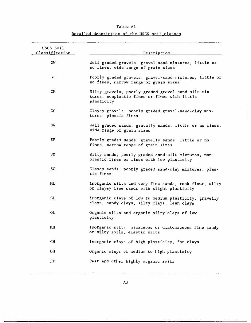
Table Al

Detailed description of the USCS soil classes

USCS SoilClassification Description

GW Well graded gravels, gravel-sand mixtures, little orno fines, wide range of grain sizes

GP Poorly graded gravels, gravel-sand mixtures, little orno fines, narrow range of grain sizes

GM Silty gravels, poorly graded gravel-sand-silt mix-tures, nonplastic fines or fines with littleplasticity

GC Clayey gravels, poorly graded gravel-sand-clay mix-tures, plastic fines

SW Well graded sands, gravelly sands, little or no fines,wide range of grain sizes

SP Poorly graded sands, gravelly sands, little or nofines, narrow range of grain sizes

SM Silty sands, poorly graded sand-silt mixtures, non-plastic fines or fines with low plasticity

SC Clayey sands, poorly graded sand-clay mixtures, plas-tic fines

ML Inorganic silts and very fine sands, rock flour, siltyor clayey fine sands with slight plasticity

CL Inorganic clays of low to medium plasticity, gravellyclays, sandy clays, silty clays, lean clays

OL Organic silts and organic silty-clays of lowplasticity

MH Inorganic silts, micaceous or diatomaceous fine sandyor silty soils, elastic silts

CH Inorganic clays of high plasticity, fat clays

OH Organic clays of medium to high plasticity

PT Peat and other highly organic soils

A3

APPENDIX B: DERIVATION OF THE CAVITY EXPANSION EQUATIONS

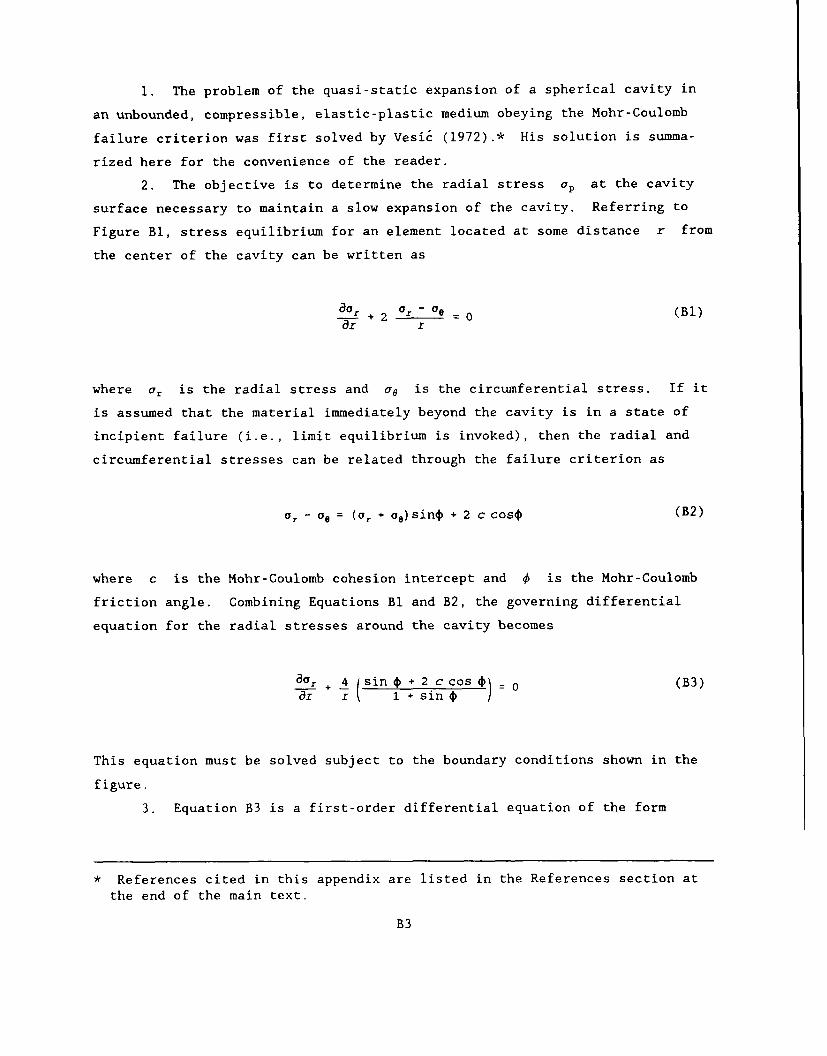
1. The problem of the quasi-static expansion of a spherical cavity in

an unbounded, compressible, elastic-plastic medium obeying the Mohr-Coulomb

failure criterion was first solved by Vesic (1972).* His solution is summa-

rized here for the convenience of the reader.

2. The objective is to determine the radial stress ap at the cavity

surface necessary to maintain a slow expansion of the cavity. Referring to

Figure Bl, stress equilibrium for an element located at some distance r from

the center of the cavity can be written as

ao __ _ - oe(I-- +2 - 0(Bl)ar r

where ar is the radial stress and u6 is the circumferential stress. If it

is assumed that the material immediately beyond the cavity is in a state of

incipient failure (i.e., limit equilibrium is invoked), then the radial and

circumferential stresses can be related through the failure criterion as

0, - Ge = (Gr + Ge) sin + 2 c coso (B2)

where c is the Mohr-Coulomb cohesion intercept and 4 is the Mohr-Coulomb

friction angle. Combining Equations Bl and B2, the governing differential

equation for the radial stresses around the cavity becomes

a8G 4 (sin 4+ 2 ccos 4) (B3)

ar r 1 + sin o

This equation must be solved subject to the boundary conditions shown in the

figure.

3. Equation B3 is a first-order differential equation of the form

* References cited in this appendix are listed in the References section at

the end of the main text.

B3

Figure Bi. Expansion of a sphericalcavity (after Vesic 1972)

d-y +P(X)-y = Q(x) (B4)dx

where

Y

dx dr

p (x) 4 . sin i)

4 (1 +cc o*

Q (x) 4 C Co 14r(I+sn

Its solution is given by

y = Ce fpx~x + eJ'P~x" f e fP (x) cx. Q xW dx (B5)

B4

where C1 is an integration constant. Applying the boundary condition a, -

Pu at r - R,, and completing the integration:

Or = (P. C cot ) )in - C cotO (B6)

This expression relates the radial stresses in the vicinity of the cavity to

the instantaneous size of the cavity and the internal cavity pressure.

4. To determine the pressure pu needed to expand the cavity to some

radius Ru , Vesic first applied the continuity condition that the change in

volume of the cavity must be equal to the change in volume of the elastic zone

plus the change in volume of the plastic zone:

R'3= ,- U +) (R,-R3)A (B7)

where up is the radial displacement of the boundary betwee- the elastic and

plastic zones, A is the average volumetric strain in the plastic zone, and

it is assumed that the initial cavity radius is zero. From elastic theory,

the displacement of the elastic/plastic boundary is proportional to the

increase in radial stress above the initial ambient pressure q

u=4(Op - q) R, B8

Substituting Equation B8 into Equation B7 and ignoring higher powers of up:

3 L- [J -2-Gc, q) +J(B9)

Substituting r - Rp in Equation B6 provides an expression for ap

B5

O (P"+ C cot t) (R i C cot4 (BlO)

Stress equilibrium requires that

(p.+ c cot)(0) Rp n c cotO (BIl)\R-)

Substituting Equations B10 and Bll into Equation B9, the following expression

for the ratio of the plastic zone radius to the cavity radius is obtained:

+ 7N _ p 3 Cos 4 + A (B12)3Vqi_ R (c + q tan )( 3 -sint, B2

Noting that for A small

and for 4 < 450

3 cos -13 - sin i

Equation B12 can be simplified and rearranged to produce the approximation

R = r (B13)-u 1+ IrA

in which Ir , the rigidity index, is equal to the ratio of the shear modulus

of the soil to its initial strength:

B6

iz _ G

c + q tan0

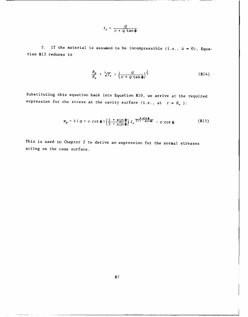
5. If the material is assumed to be incompressible (i.e., A - 0), Equa-

tion B13 reduces to

_P= r1 (B14)R,, c + q tan

Substituting this equation back into Equation B1O, we arrive at the requiredexpression for the stress at the cavity surface (i.e., at r - R, ):

4 ain*

up 3 (q + c cot )(i+S fln)I0) 3 C Ccot, (B15)

This is used in Chapter 2 to derive an expression for the normal stresses

acting on the cone surface.

B7

APPENDIX C: A FORTRAN IMPLEMENTATION OF THE METHODOLOGY

CC Binary Iteration Routine for Solving Cone Index Equation

CCC INPUT VARIABLESCC Width - Maximum cone diameter in inches (real)C USCS - USCS soil classification (2-character string)C Z - Cone index measurement depth in inches (real)C CI - Measured cone index in psi (real)CC OUTPUT VARIABLESCC Density - Relative density in percent (real)C Gamma - Dry unit weight in pcf (real)C Phi - Friction angle in degrees (real)C G - Elastic shear modulus in psi (real)C * Alternate return for error conditionCC LOCAL VARIABLESCC Soil - Soil type index into Angles and Gammas arrays (integer)C Lower - Density index into Angles and Gammas arrays (integer)C Angles - Array of friction angles for each soil type (real)C Gammas - Array of unit weights for each soil type (real)C Symbol - Array of USCS soil classification symbols (character*2)C E - Void ratio (real)C AngleG - Shear modulus for angular soils in psi (real)C RoundG - Shear modulus for rounded soils in psi (real)C Predict - Computed cone index in psi (real)CC

Subroutine SOLVER (USCS,Z,CI,Density,Gamma,Phi,G,*)

Integer Soil,LowerReal Angles(5,6),Gammas(5,6)Real Width,Z,CI,Phi,G,Gamma,E,DensityReal Increment,Ratio,Delta,Fuzz,AngleG,RoundG,PredictCharacter USCS*2,Symbol*2(2,6)

Data Symbol / 'gw' 'GW'1 'gp' 'GP'2 'sw' 'SW'3 'sm' 'SM'4 $sp' ISP'

5 'ml' 'ML' /

Data Angles / 27.9 31.4 36.0 40.1 45.01 27.5 30.7 34.6 38.3 42.52 27.1 30.1 33.6 37.0 40.73 26.9 29.7 32.9 35.9 39.14 26.4 29.1 31.9 34.7 37.85 25.9 28.4 31.1 33.4 36.0 /

Data Gammas /117.7 ,123.3 ,130.6 ,138.1 ,147.71 109.0 ,114.0 ,120.0 ,126.6 ,133.7

C3

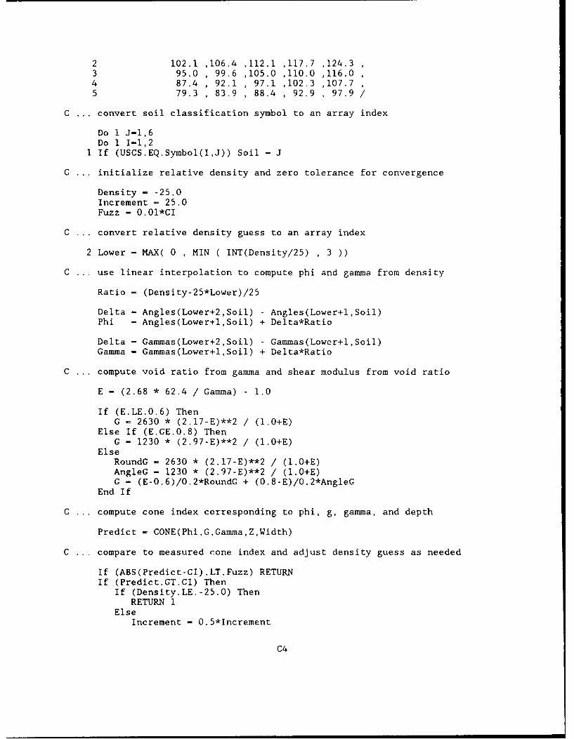
2 102.1 .106.4 ,112.1 ,117.7 ,124.33 95.0 ,99.6 ,105.0 ,110.0 ,116.04 87.4 ,92.1 ,97.1 ,102.3 ,107.75 79.3 ,83.9 ,88.4 , 92.9 ,97.9/

C ... convert soil classification symbol to an array index

Do 1 J-1,6Do 1 1-1,2

1 If (USCS.EQ.Symbol(I,J)) Soil - J

C ... initialize relative density and zero tolerance for convergence

Density - -25.0Increment - 25.0Fuzz - 0.Ol*GI

C ... convert relative density guess to an array index

2 Lower - MAX( 0 , MIN ( INT(Density/25) , 3 ))

C ... use linear interpolation to compute phi and gamma from density

Ratio - (Density-25*Lower)/25

Delta - Angles(Lower+2,Soil) - Angles(Lower+l,Soil)

Phi - Angles(Lower+l,Soil) + Delta*Ratio

Delta - Gammas(Lower+2,Soil) - Gammas(Lower+l,Soil)

Gamma - Gammas(Lower+l,Soil) + Delta*Ratio

C .. compute void ratio from gamma and shear modulus from void ratio

E - (2.68 * 62.4 / Gamma) -1.0

If (E.LE.0.6) ThenG - 2630 * (2.17-E)**2 /(1.0+E)

Else If (E.GE.0.8) ThenG - 1230 * (2.97-E)**2 /(1.0+E)

ElseRoundG - 2630 * (2.17-E)**2 /(l.0+E)AngleG - 1230 * (2.97-E)**2 /(1.0+E)G - (E-0.6)/0.2*RoundG + (0.8-E)/0.2*AngleG

End If

C ... compute cone index corresponding to phi, g, gamma, and depth

Predict - CONE(Phi,G,Gamma,Z,Width)

C . .. compare to measured cone index and adjust density guess as needed

If (ABS(Predict-CI).LT.Fuzz) RETURN~If (Predict.GT.CI) Then

If (Density.LE. -25.0) ThenRETURN 1

ElseIncrement - 0.5*Increment

C4

Density - Density - IncrementEnd If

ElseIf (Density.GE.150.O) Then

RETURN IElse

Density = Density + IncrementEnd If

End If

C ... compute another cone index estimate using the new relative density

Go To 2

End

C5

C-- - - - -- - -- - - - -C Mathematical Model for Computing Cone IndexCCC INPUTCC Phi - Friction angle in degrees (real)C G - Elastic shear modulus in psi (real)C Gamma - Dry unit weight in pcf (real)C Z - Cone index measurement depth in inches (real)C Width - Maximum cone diameter in inches (real)CC - - - - - - - - - - - - - - - - - - - - - - - - - - - - - - - - -

Function CONE(Phi,G,Gamma,Z,Width)

Parameter (Alpha=15.O,A=O.986,B=lOO.O,Beta=O.55)

Double Precision CammaTanPhi ,Terml ,Term2 ,OmegaReal Phi,G,Gaxr.;.-a,Z,Pi ,TanAlpha,SinPhi ,TanPhi,H,M,Ga

C ... compute cone height from width and apex angle

Pi - ATAN2(O.0,-l.O)TanAlpha -TAN(Pi*Alpha/180)H - O.5*Width/TanAlpha

C . .. compute trig functions involving friction angle

SinPhi - SIN(Pi*Phi/180)TanPhi - TAN(Pi*Phi/180)GammaTanPhi - (Gamma/1728)*TanPhi

C ... compute the exponent of the shear modulus

M - 4./3. * SinPhi/(l.+SinPhi)

C ... compute the omega term

Terml - ((Z-sH)*GammaTanPhi)**(3-M)Term2 - (Z+(3-M)*H) * GammaTanPhi * (Z*GammaTanPhi)**(2-M)Omega = (Terml-Term2) / (2-M) / (3-M) / (H*GammaTanPhi)**2

C ... adjust the shear modulus for free surface effects

Ca - 0.5 * C * (A + (1. -B*EXP(-Beta*Z)) / (l.+B*EXP(-Beta*Z)))

C ... compute and return the cone index

CONE - 6 * Ga**M * Omega1 * (l.+SinPhi) / (3. -SinPhi)2 * (TanAlpha+TanPhi) / (TanAlpha*TanPhi)

ReturnEnd

C6

APPENDIX D: NOTATION

A Empirical constant used to calculate apparent shear modulus

B Empirical constant used to calculate apparent shear modulus

c Mohr-Coulomb cohesion intercept

C, Constant of integration

CI Cone index (cone penetration resistance)

Dr Relative density of the soil

E Coefficient of angularity of the soil grains

e Void ratio of the soil

F7 Measured vertical force on the cone

G Initial elastic shear modulus of the soil

Ga Apparent shear modulus (adjusted for free-surface effects)

GC Specific gravity of the soil

Ir Rigidity index of the soil

L Length of the cone tip

m Shear modulus exponent in the cone index equation

n Porosity of the soil

Pu Pressure inside a spherical cavity of arbitrary radius

q Overburden stress at an arbitrary depth

r Arbitrary radius of the cone tip

Ru Arbitrary radius of an expanding spherical cavity

Rp Arbitrary radius of the plastic zone around the cavity

UP Arbitrary displacement of the elastic-plastic boundary

Z Depth of cone penetration

a Apex angle of the cone tip

Empirical constant used to calculate apparent shear modulus

A Volumetric strain in the vicinity of the cavity

Total unit weight of the soil

-1d Dry unit weight of the soil

7w Unit weight of water

?Arbitrary vertical distance from the cone tip

a Arbitrary normal stress acting on the cone tip

a, In situ confining presiure

Cp Pressure inside an expanding spherical cavity

a, Arbitrary radial stress

ae Arbitrary circumferential stress

D3

r Arbitrary shear stress acting on the cone tip

Mohr-Coulomb friction angle

(Term used to simplify the cone index equation

D4

Waterways Experiment Station Cataloging-In-Publication Data

Perkins, William E.Strength property estimation for dry cohesionless soils using the mili-

tary cone penetrometer / by William E. Perkins and Roger W. Meier,John V. Farr ; prepared for Department of the Army, U.S. Army Corps ofEngineers.

51 p. : ill. ; 28 cm. -- (Technical report ; GL-92-5)Includes bibliographic references.1. Trafficability. 2. Soil penetration test. 3. Soil mechanic. 4. Tires,

Rubber -- Traction. I. Title. II. Meier, Roger W. Ill. Meier, Roger W.IV. United States. Army. Corps of Engineers. V. U.S. Army EngineerWaterways Experiment Station. VI. Series: Technical report (U.S. ArmyEngineer Waterways Experiment Station) ; GL-92-5.TA7 W34 no.GL-92-5