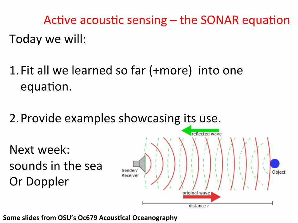
Ac#ve  acous#c  sensing  –  the  SONAR  equa#on  Today  we  will:    1. Fit  all  we  learned  so  far  (+more)    into  one  equa#on.  

2. Provide  examples  showcasing  its  use.    Next  week:    sounds  in  the  sea  Or  Doppler  

Some  slides  from  OSU’s  Oc679  Acous5cal  Oceanography  

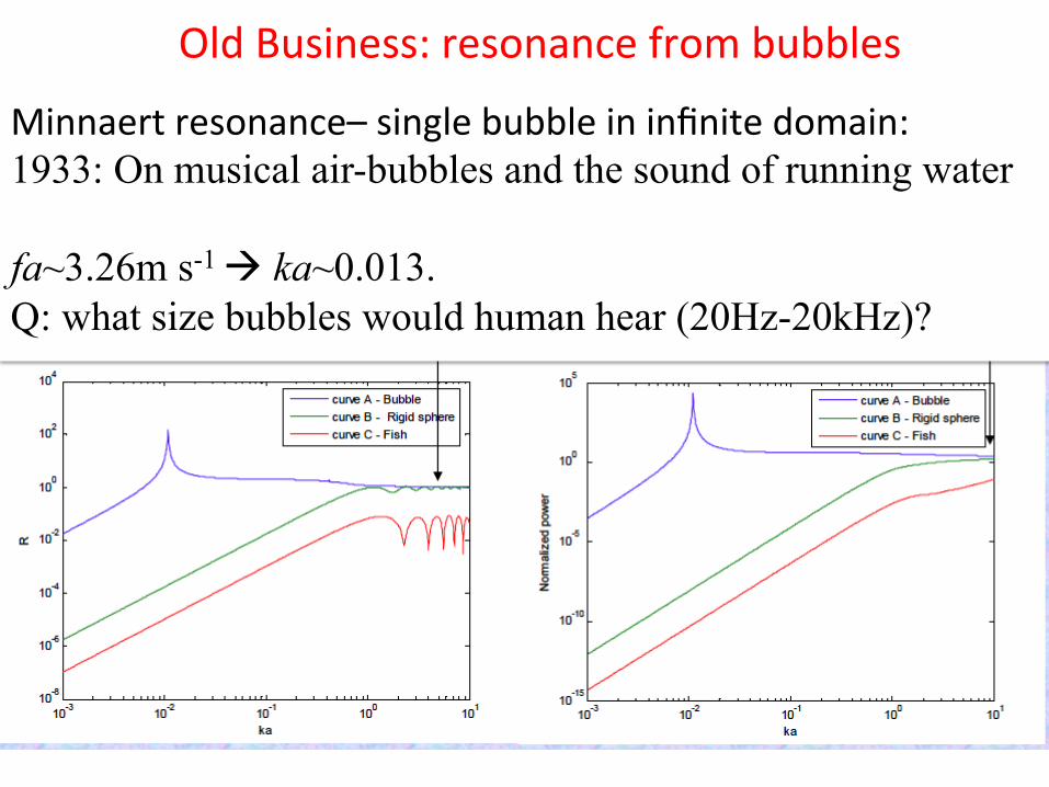
Old  Business:  resonance  from  bubbles  

Πs =1

Minnaert  resonance–  single  bubble  in  infinite  domain:  1933: On musical air-bubbles and the sound of running water    fa~3.26m s-1 à ka~0.013. Q: what size bubbles would human hear (20Hz-20kHz)?

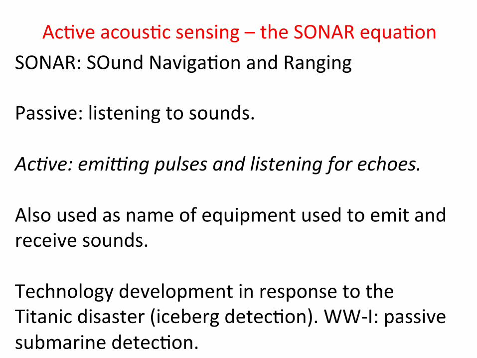
Ac#ve  acous#c  sensing  –  the  SONAR  equa#on  SONAR:  SOund  Naviga#on  and  Ranging    Passive:  listening  to  sounds.    Ac#ve:  emi*ng  pulses  and  listening  for  echoes.    Also  used  as  name  of  equipment  used  to  emit  and  receive  sounds.    Technology  development  in  response  to  the  Titanic  disaster  (iceberg  detec#on).  WW-­‐I:  passive  submarine  detec#on.  

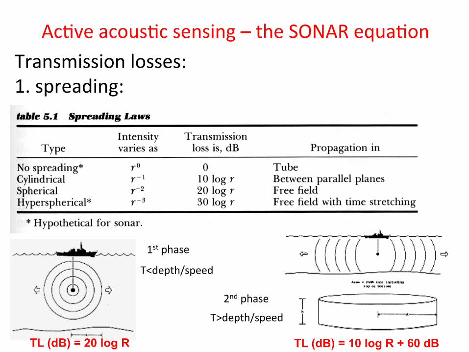
Ac#ve  acous#c  sensing  –  the  SONAR  equa#on  Transmission  losses:  1.  spreading:    

1st  phase  

2nd  phase  

T<depth/speed  

T>depth/speed  

TL (dB) = 20 log R TL (dB) = 10 log R + 60 dB

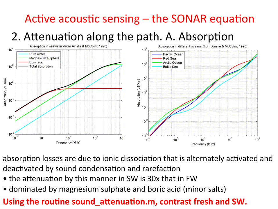
Ac#ve  acous#c  sensing  –  the  SONAR  equa#on    2.  AUenua#on  along  the  path.  A.  Absorp#on    

absorp#on  losses  are  due  to  ionic  dissocia#on  that  is  alternately  ac#vated  and  deac#vated  by  sound  condensa#on  and  rarefac#on      •   the  aUenua#on  by  this  manner  in  SW  is  30x  that  in  FW  •   dominated  by  magnesium  sulphate  and  boric  acid  (minor  salts)  Using  the  rou5ne  sound_a>enua5on.m,  contrast  fresh  and  SW.    

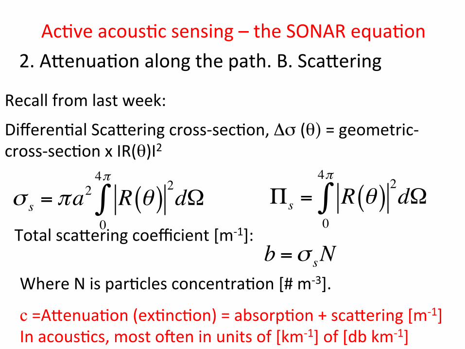
Ac#ve  acous#c  sensing  –  the  SONAR  equa#on    2.  AUenua#on  along  the  path.  B.  ScaUering    

Recall  from  last  week:      

Differen#al  ScaUering  cross-­‐sec#on,  Δσ (θ) =  geometric-­‐cross-­‐sec#on  x  IR(θ)I2    

σ s = πa2 R θ( )

2

0

4π

∫ dΩ Πs = R θ( )2

0

4π

∫ dΩ

b =σ sNTotal  scaUering  coefficient  [m-­‐1]:  

Where  N  is  par#cles  concentra#on  [#  m-­‐3].  

c  =AUenua#on  (ex#nc#on)  =  absorp#on  +  scaUering  [m-­‐1]  In  acous#cs,  most  o`en  in  units  of  [km-­‐1]  of  [db  km-­‐1]  

Ac#ve  acous#c  sensing  –  the  SONAR  equa#on  

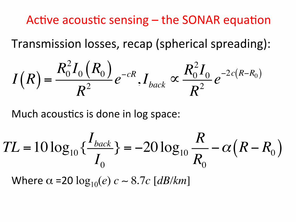
Transmission  losses,  recap  (spherical  spreading):  

I R( ) =R02I0 R0( )R2

e−cR, Iback ∝R02I0R2

e−2c R−R0( )

TL =10 log10{IbackI0} = −20 log10

RR0−α R− R0( )

Much  acous#cs  is  done  in  log  space:  

Where  α  =20  log10(e) c ∼ 8.7c [dB/km]

Ac#ve  acous#c  sensing  –  the  SONAR  equa#on  

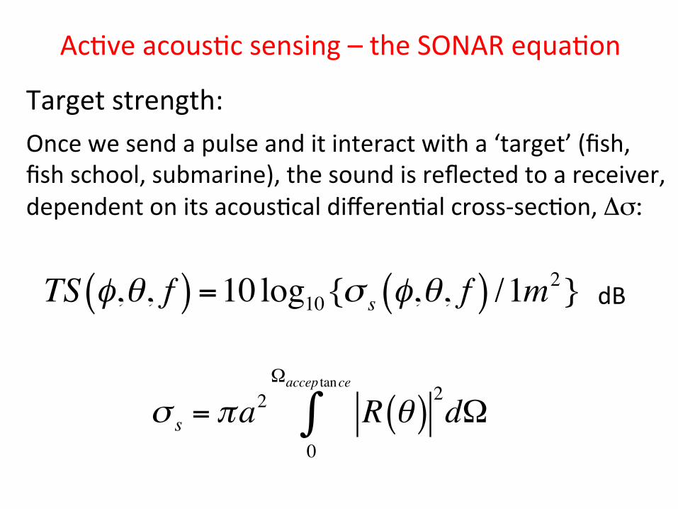
Target  strength:  

TS φ,θ, f( ) =10 log10{σ s φ,θ, f( ) /1m2}

Once  we  send  a  pulse  and  it  interact  with  a  ‘target’  (fish,  fish  school,  submarine),  the  sound  is  reflected  to  a  receiver,  dependent  on  its  acous#cal  differen#al  cross-­‐sec#on,  Δσ:  

dB

σ s = πa2 R θ( )

2

0

Ωaccep tance

∫ dΩ

Ac#ve  acous#c  sensing  –  the  SONAR  equa#on  

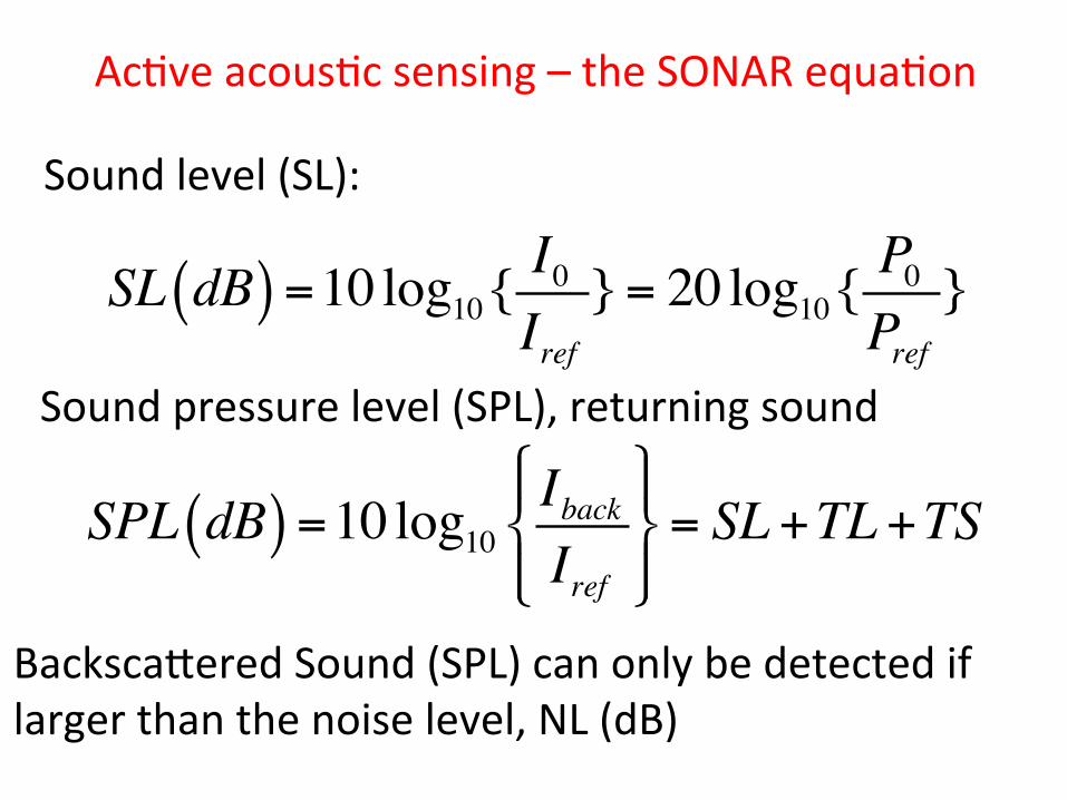
Sound  level  (SL):    SL dB( ) =10 log10{

I0Iref} = 20 log10{

P0Pref}

Sound  pressure  level  (SPL),  returning  sound  

SPL dB( ) =10 log10IbackIref

!"#

$#

%&#

'#= SL +TL +TS

BackscaUered  Sound  (SPL)  can  only  be  detected  if  larger  than  the  noise  level,  NL  (dB)  

Ac#ve  acous#c  sensing  –  the  SONAR  equa#on  

Some  illustra#ve  problems:    1.  Close  to  the  source,  as  we  double  the  distance,  

what  is  the  TL  for  a  low  frequency  sound?  

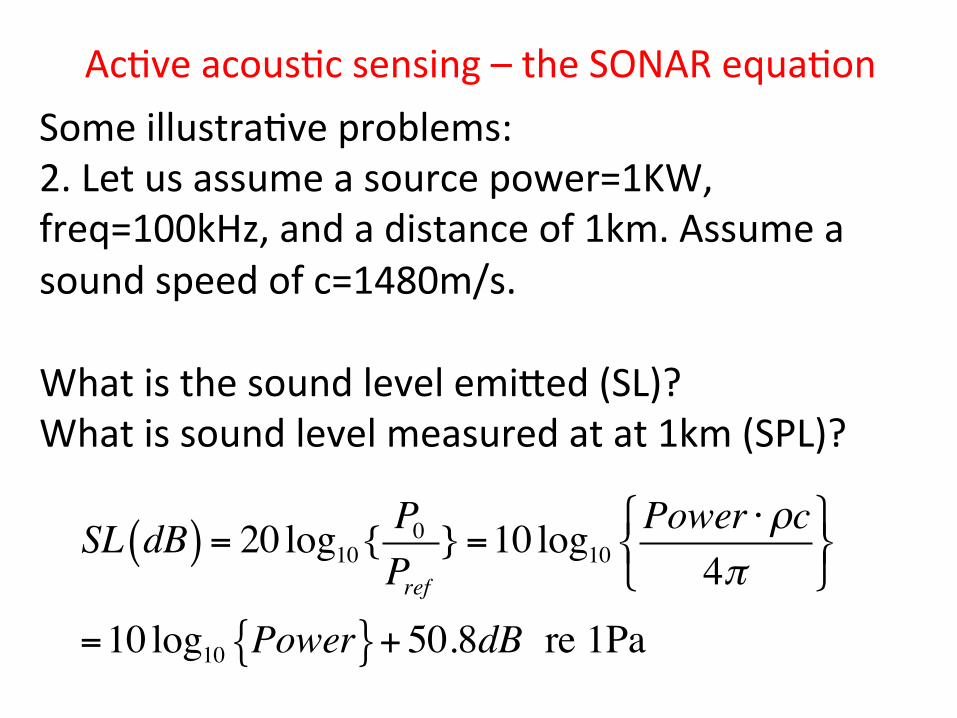
Ac#ve  acous#c  sensing  –  the  SONAR  equa#on  Some  illustra#ve  problems:  2.  Let  us  assume  a  source  power=1KW,  freq=100kHz,  and  a  distance  of  1km.  Assume  a  sound  speed  of  c=1480m/s.    What  is  the  sound  level  emiUed  (SL)?  What  is  sound  level  measured  at  at  1km  (SPL)?  

SL dB( ) = 20 log10{ P0

Pref} =10 log10

Power ⋅ρc4π

"#$

%&'

=10 log10 Power{ }+ 50.8dB re 1Pa

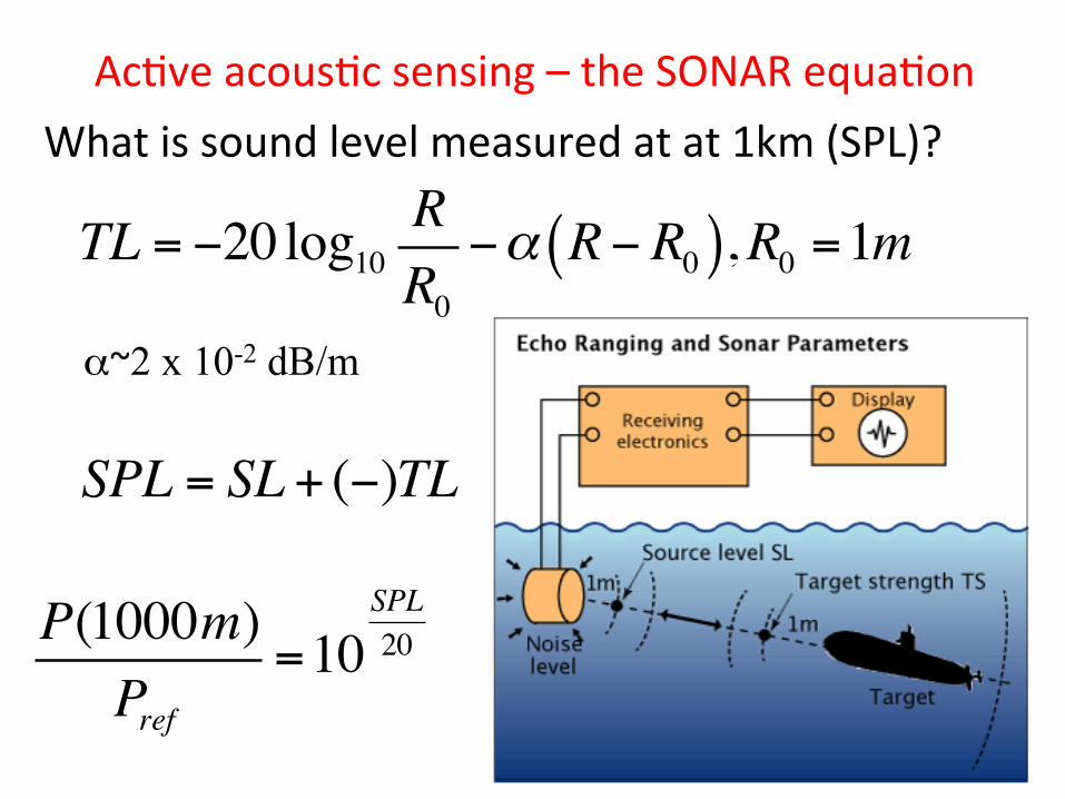
Ac#ve  acous#c  sensing  –  the  SONAR  equa#on  What  is  sound  level  measured  at  at  1km  (SPL)?  

TL = −20 log10RR0−α R− R0( ),R0 =1m

α~2 x 10-2 dB/m

SPL = SL + (−)TL

P(1000m)Pref

=10SPL20

13

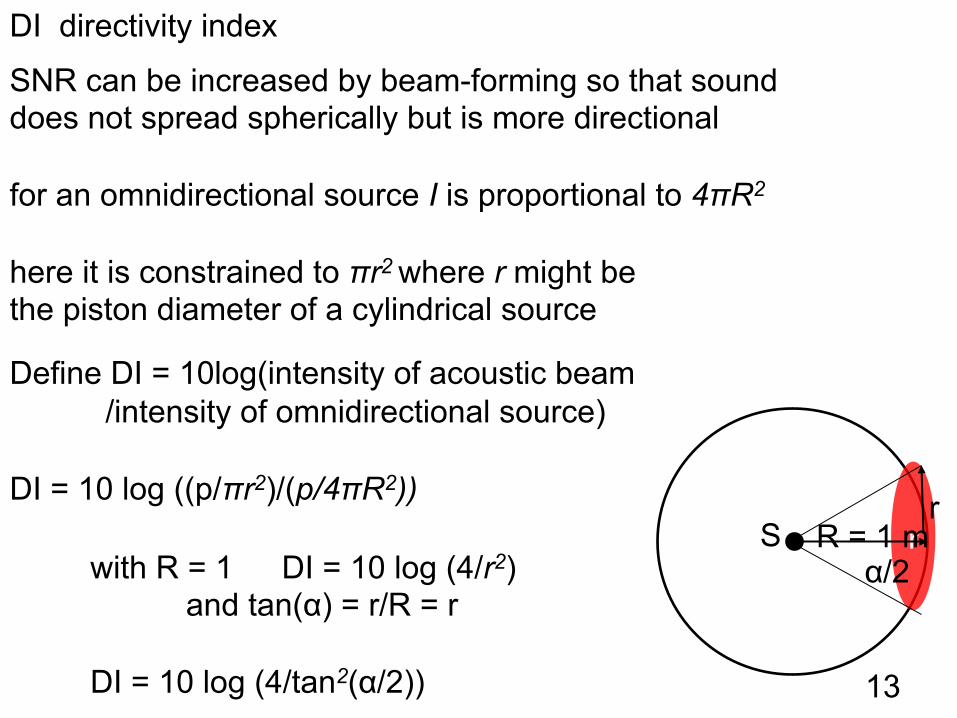
SNR can be increased by beam-forming so that sound does not spread spherically but is more directional for an omnidirectional source I is proportional to 4πR2

here it is constrained to πr2 where r might be the piston diameter of a cylindrical source

Define DI = 10log(intensity of acoustic beam /intensity of omnidirectional source)

DI = 10 log ((p/πr2)/(p/4πR2))

S r  R = 1 m r

α/2 with R = 1 DI = 10 log (4/r2) and tan(α) = r/R = r

DI = 10 log (4/tan2(α/2))

DI directivity index

14

SNR can be increased by beam-forming produced by an array of transducers (perhaps in a single head or maybe distributed geographically) the directivity index DI represents this advantage for a particular array so that

SNR = SL + TL – N + DI N-noise ideally, detection is possible when the signal is sufficiently close and not disguised by noise …

that is, when SNR > 0 however, due to the nature of the signal, interference, the sonar operator’s training and alertness, etc … something more than 0 is necessary this extra appears as a detection threshold, DT we now write the SONAR EQUATION in terms of a signal excess SE

SE = SL + TL – N + DI – DT this is now the difference between the actual received signal at the output of the beamformed array and minimum signal required for detection

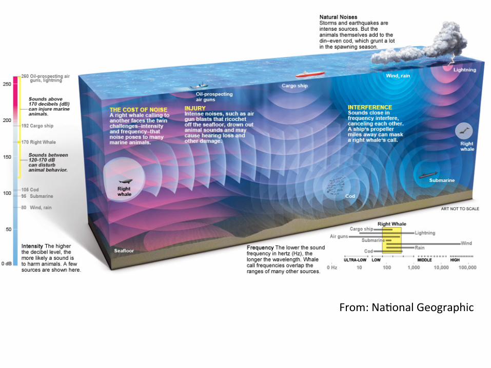
From:  Na#onal  Geographic  

Example  of  underwater  sounds:    Earthquake  [movie]    Rain  [website]    Breaking  waves  [website]    Ice  grinding  on  seafloor  [website]    Man  made  [website]    Marine  mammals  [website],  fish  [website]    

Wenz  diagram:  

From:  hUp://www.dosits.org/  

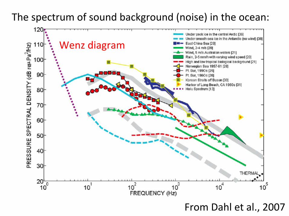
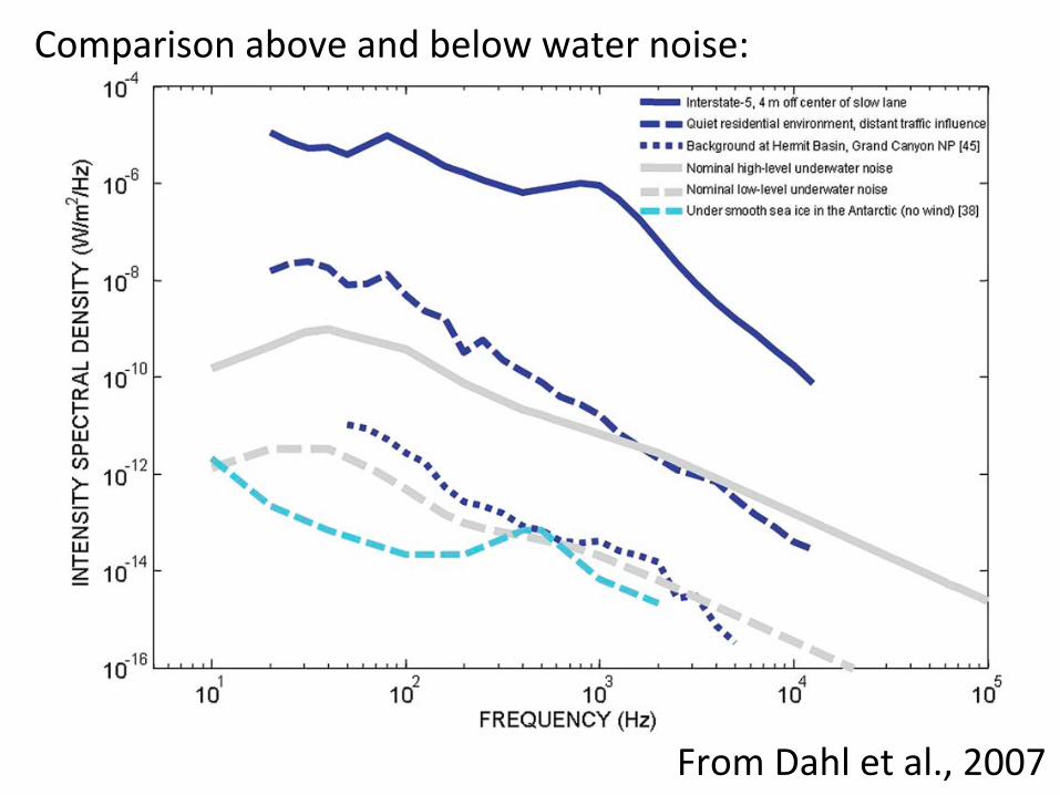
The  spectrum  of  sound  background  (noise)  in  the  ocean:  

Wenz  diagram  

From  Dahl  et  al.,  2007  

From  Dahl  et  al.,  2007  

Comparison  above  and  below  water  noise:  

20

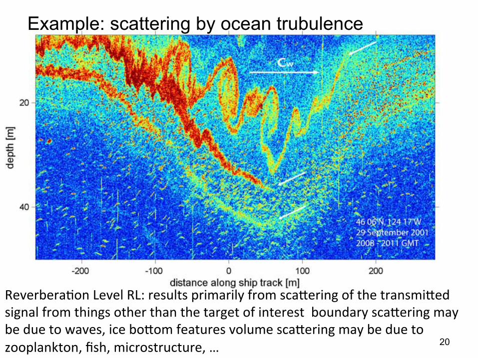
Example: scattering by ocean trubulence

Reverbera#on  Level  RL:  results  primarily  from  scaUering  of  the  transmiUed    signal  from  things  other  than  the  target  of  interest    boundary  scaUering  may  be  due  to  waves,  ice  boUom  features  volume  scaUering  may  be  due  to  zooplankton,  fish,  microstructure,  …  

So,  there  are  essen#ally  two  types  of  background  that  may  mask  the  signal  that  we  wish  to  detect:      

1) Noise  background  or  Noise  Level  (NL).  This  is  an  essen#ally  a  steady  state,  isotropic  (equal  in  all  direc#ons)  sound  which  is  generated  by  amongst  other  things  wind,  waves,  biological  ac#vity  and  shipping.  This  is  in  addi#on  to  transducer  system  self-­‐noise.  (Wenz  curves)  

2)  Reverbera5on  background  or  reverbera#on  level  (RL).  This  is  the  slowly  decaying  por#on  of  the  back-­‐scaUered  sound  from  one's  own  acous#c  input.  Excellent  reflectors  in  the  form  of  the  sea  surface  and  floor  bound  the  ocean.  Addi#onally,  sound  may  be  scaUered  by  par#culate  maUer  (e.g.  plankton)  within  the  water  column.  You  will  have  experienced  reverbera#on  for  yourself.  For  example  if  you  shout  loudly  in  a  cave  you  are  likely  to  here  a  series  of  echoes  reverbera#ng  due  to  sound  reflec#ons  from  the  hard  rock  surfaces.  These  reverbera#ons  decay  rapidly  with  #me.    

22

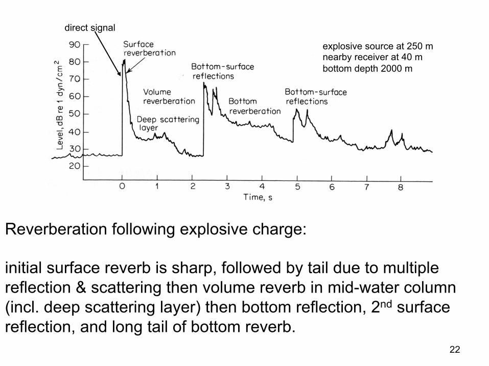
Reverberation following explosive charge: initial surface reverb is sharp, followed by tail due to multiple reflection & scattering then volume reverb in mid-water column (incl. deep scattering layer) then bottom reflection, 2nd surface reflection, and long tail of bottom reverb.

explosive source at 250 m nearby receiver at 40 m bottom depth 2000 m

direct signal

23

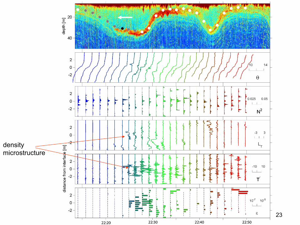
density microstructure

24

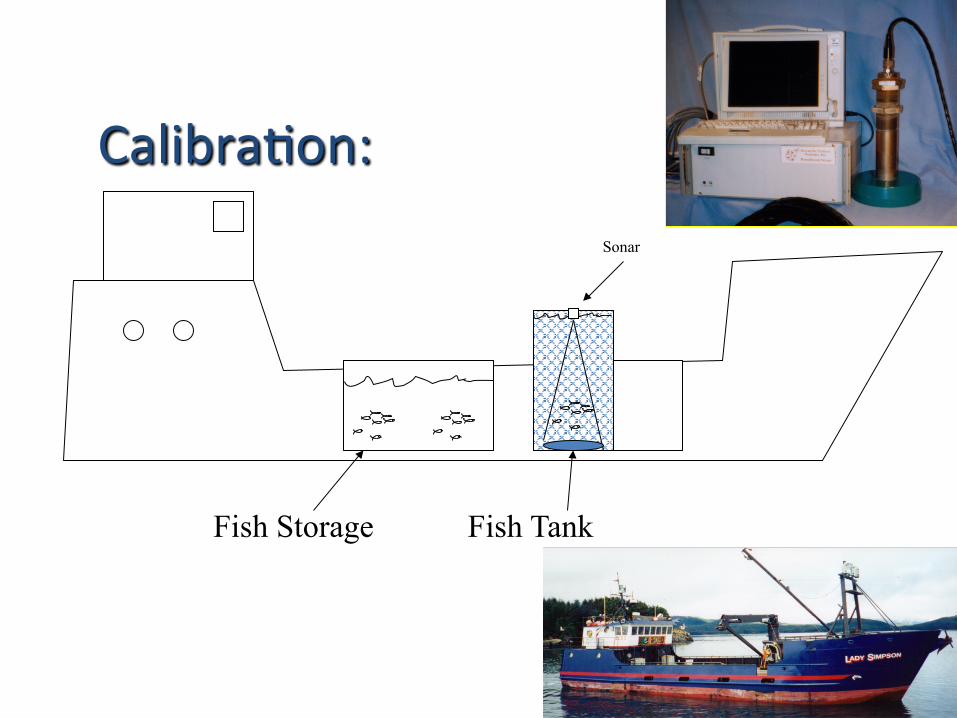
Fish Storage Fish Tank

Sonar

Calibra#on:  

11/6/12 SMS 204: Integrative Marine Sciences II 25

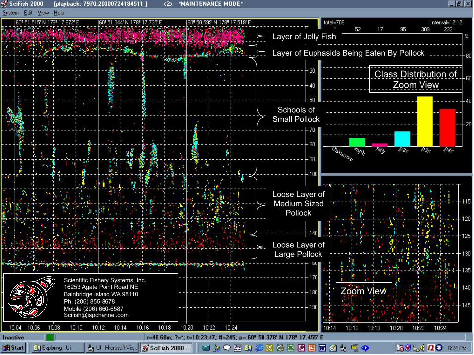
SciFish 2000: Broadband Fish ID Sonar

Layer of Jelly Fish

Layer of Euphasids Being Eaten By Pollock

Schools of Small Pollock

Loose Layer of Medium Sized

Pollock

Loose Layer of Large Pollock

Zoom View

Class Distribution of Zoom View

Scientific Fishery Systems, Inc. 16253 Agate Point Road NE Bainbridge Island WA 98110 Ph. (206) 855-8678 Mobile (206) 660-6587 Scifish@ispchannel.com

26