Acts of God? Religiosity and Natural Disasters

Across Subnational World Districts

Jeanet Sinding Bentzen∗

Department of Economics, University of Copenhagen

September 6, 2018

Abstract

Religious beliefs influence individual behavior in many settings. But why are

some societies more religious than others? One answer is religious coping: Indi-

viduals turn to religion to deal with unbearable and unpredictable life events. To

investigate whether coping can explain global differences in religiosity, I combine

a global dataset on individual-level religiosity with spatial data on natural disas-

ters. Individuals become more religious if an earthquake recently hit close by. Even

though the effect decreases after a while, data on children of immigrants reveal a

persistent effect across generations. The results point to religious coping as the main

mediating channel, but alternative explanations such as mutual insurance or migra-

tion cannot be ruled out entirely. The findings may help explain why religiosity has

not vanished as some scholars once predicted.

∗Jeanet.Bentzen@econ.ku.dk. I would like to thank Pelle Ahlerup, Philipp Ager, Thomas BarnebeckAndersen, Robert Barro, Roland Bénabou, Daniel Chen, Antonio Ciccone, Carl-Johan Dalgaard, ThomasDohmen, Ernst Fehr, Oded Galor, Nicola Gennaioli, Casper Worm Hansen, Noel D. Johnson, Jo ThoriLind, Anastasia Litina, Benjamin Marx, Andrea Matranga, Stelios Michalopoulos, Omer Moav, BenjaminOlken, Ola Olsson, Luigi Pascali, Giacomo Ponzetto, Sarah Smith, Hans-Joachim Voth, Asger Mose Win-gender, Fabrizio Zilibotti, Yanos Zyllerberg, seminar participants at University of Luxembourg, Universityof Bonn, New Economic School, Bristol University, University of Zurich, University of Gothenburg, OsloUniversity, University of Copenhagen, and participants at the conference on "The Future Directions onthe Evolution of Rituals, Beliefs and Religious Minds", the ASREC conference, the AEA Annual Meeting,the NBER Summer Institute, the WEHC, GSE Summer Forum in Barcelona, the European EconomicAssociation Annual Congress, and the Nordic Conference in Development Economics for comments. Thispaper is a major revision of Bentzen (2013), which benefited from financial support from the CarlsbergFoundation.

1 IntroductionMore than four out of every five people on Earth profess a belief in God. There are large

differences from country to country: Believers vary from 20% of the population in China

to 100% in Algeria and Pakistan. There are also large differences within countries: 2%

in Shanghai and 60% in the Fujian province.1 These differences in religiosity matter for

economic outcomes, such as labour force participation, education, crime, redistribution

policies, health, and possibly even aggregate outcomes such as GDP per capita growth.2

A first-order question is why some societies are more religious than others.

I test whether the need to cope psychologically with adverse shocks is an important

determinant of differences in religiosity. This is known as the religious coping hypoth-

esis. The hypothesis states that individuals draw on religious beliefs and practices to

understand and deal with unbearable and unpredictable situations.3 People seek a closer

relationship with God or they find a reason for the event by attributing it to an act of

God. Believers often answer that coping with adversity is one of the main purposes of re-

ligion, and scholars have emphasized that all major religions potentially provide coping.4

Indeed, Karl Marx and Sigmund Freud maintained that all religions evolved to provide

individuals with a higher power to turn to in times of hardship.5

I use natural disasters as a determinant of unpredictable adverse life events. I combine

data on natural disasters with the pooled World Values Survey and European Values

Study, available for 424,099 individuals in 96 countries. The surveys ask questions such

as "How important is God in your life?" and "Are you a religious person?" The surveys

also hold information on the location of the interview at the subnational district level.

Each individual can therefore be matched with disasters at the district level. This allows

inclusion of country fixed effects in the empirical analysis, which means that religiosity

is compared only within countries, instead of across. I investigate mainly earthquakes,

as earthquakes have proven very diffi cult to predict and since data on earthquakes are

1Source: The pooled World Values Survey and European Values Study 2004-2014.2See Guiso et al. (2003), Scheve & Stasavage (2006), McCleary & Barro (2006), Gruber & Hungerman

(2008), and Campante & Yanagizawa-Drott (2015) for empirical investigations or Iannaccone (1998),Lehrer (2004), Iyer (2016), and Kimball et al. (2009) for reviews.

3E.g., Pargament (2001), Cohen & Wills (1985), Park et al. (1990), Williams et al. (1991).4Clark (1958) and Pargament (2001).5Feuerbach (1957), Freud (1927), and Marx (1867).

1

particularly reliable.6 Across 600-850 subnational districts of the world, individuals in

districts with higher earthquake risk are more religious than those living in areas with

lower earthquake risk. The binned scatterplot in Figure 1 shows the simple within-country

relation between religiosity and the main measure of earthquake risk, distance to high-risk

earthquake zones.

Figure 1. Binned scatterplot of the within-country relation between earthquake risk and religiosity in 50 bins

The main analysis uses six survey-based measures of religiosity that span global re-

ligiosity. The result is robust to adding controls for various individual characteristics as

well as district-level geographic and economic confounders. Other unpredictable disasters

such as volcanic eruptions and tsunamis also increase district-level religiosity. Individuals

living on every continent and belonging to all major denominations, except Buddhism,

respond to higher disaster risk by increased religiosity. A one standard deviation increase

in earthquake risk increases religiosity by 8-11% of a standard deviation. This amounts

to 80% of the well-established gender difference in religiosity.7

The result extends to measures of religiosity that are not based on surveys. People

google "God", "Jesus", "the Bible", and "Pray" more often in US states with higher

earthquake risk, compared to states with lower risk of earthquakes.

One concern is that unobserved factors are left out of the analysis, biasing the results.

I exploit the time-dimension of the data to construct a panel where districts are followed

over time. District-level religiosity increases after a recent earthquake. The effect is

6Fisker (2012). Other types of disasters such as wars, economic crises, and epidemic diseases areendogenous to various factors and thus unsuitable as natural experiments.

7Numerous studies have shown that women are more religious than men (see review by Trzebiatowska& Bruce (2012)).

2

due to increased personal beliefs and not increased churchgoing. The result is robust

to adding country-by-year fixed effects, individual level controls, and reassuringly, future

earthquakes do not affect current religiosity. Religiosity increases more in districts with

lower average incomes, education, and population densities. Consistent with a literature

on dynamic effects of various shocks on cultural values, the short-term spike in religiosity

abates with time.8

To investigate whether a persistent residual impact remains, the last part of the analy-

sis combines data on second generation immigrants with earthquake risk in their parents’

country of origin. Individuals with parents from countries with high earthquake risk are

more religious than those with parents from low earthquake risk areas. The result is ro-

bust to including country of residence fixed effects (picking up e.g., earthquake risk and

average religiosity in the country of residence) and to adding controls at the level of the

individual, parent, and country of origin. It seems that living in high-risk earthquake

areas intensifies religiosity, which is passed on to future generations, like cultural values.

The analysis proceeds to investigate the mechanism through which earthquakes influ-

ence religiosity. Alternative explanations involving the direct economic loss after earth-

quakes, migration/selection, or a special culture evolving in high-risk areas, can explain

some of the results. But only religious coping can explain all results across all analyses.

The findings relate to a literature that investigates the long-run emergence of poten-

tially useful beliefs. This literature has linked gender roles to past agricultural practices

(Alesina et al. (2013)), individualism to past trading strategies (Greif (1994)), trust to

the slave trade in Africa and climatic risk (Nunn & Wantchekon (2011), Buggle & Du-

rante (2017)), time-preference to variation in land productivity (Galor & Özak (2016)),

and anti-Semitism to the Black Death (Voigtländer & Voth (2012)). The current study

links a cultural value with evident implications for economic outcomes (religiosity) to one

of its potential roots: Disaster risk.

The paper also relates to a literature that investigates cultural change caused by

various shocks. Such shocks could be slave trade, climatic risk, and the Black Death

from the above-mentioned studies. Another example is the Protestant Reformation (e.g.,

Becker & Woessmann (2009), Cantoni (2015), Andersen et al. (2017)), which influenced

cultural values, such as hard work. The current study investigates earthquakes as such a

8E.g., Perrin & Smolek (2009) and Dinesen & Jæger (2013).

3

shock.

Last, the paper relates to a literature investigating the role of various socio-economic

and psychological factors for differences in religiosity. For instance, studies have docu-

mented an increase in religiosity after other negative shocks, such as unemployment and

divorce (Clark & Lelkes (2005)), declining social mobility (Binzel & Carvalho (2017)),

rainfall variability (Ager & Ciccone (2018)), income shocks (Dehejia et al. (2007)), and

the financial crisis (Chen (2010)).9 The former two studies interpret religion as a psy-

chological coping mechanism. The latter three studies interpret religion as a physical

insurance mechanism, where people gain material aid by going to church. I attempt to

disentangle these mechanisms empirically. For instance, the empirical setup makes it pos-

sible to remove districts that are directly damaged by earthquakes. The remaining effect

can therefore not be attributed to physical insurance mechanisms or other explanations

relating to direct development effects. One potential exception is if people choose to go to

church in neighbouring districts to obtain material aid. This effect is also ruled out em-

pirically in the event study, where churchgoing is not affected by earthquakes. I perform

additional mechanism checks.

2 Religious copingReligious coping means using religion psychologically to cope with unbearable and unpre-

dictable situations.10 Religious coping can involve seeking a closer relationship with God

through prayer or other religious acts or finding a reason for the event by attributing it

to an act of God. Religious coping is an example of emotion-focused coping, which aims

at reducing or managing the emotional distress arising from the situation.

People say they use religion in coping. Nine out of ten Americans in a survey reported

that they coped with their distress after the September 11 attack by turning to their

religion (Schuster et al. (2001)). Many of the victims of the 1993 Mississippi River floods

reported that religious stories, the fellowship of church members, and strength from God

helped them endure and survive the flood (Smith et al. (2000)). Empirical evidence shows

that individuals hit by various adverse life events, such as cancer, heart problems, death

9On the contrary, Buser (2015) documents a positive income shock that increased churchgoing inEcuador.10E.g., Pargament (2001), Cohen & Wills (1985), Park et al. (1990), Williams et al. (1991).

4

in close family, alcoholism, divorce, or injury are more religious than others.11 Prayer

is often a preferred coping strategy by hospitalized patients above seeking information,

going to the doctor, or taking prescription drugs (Conway (1985)). However, being hit

by adverse life events is most likely correlated with unobserved individual characteristics

(such as lifestyle), which in turn may matter for one’s inclination to be religious.

Norenzayan & Hansen (2006) solved the endogeneity issue in an experiment with 28

students from the University of Michigan. They primed half of the students with thoughts

of death and the other half with neutral thoughts.12 After the experiment, the students

primed with thoughts of death were more likely to reveal religious beliefs. While solving

the endogeneity issue, the study’s external validity is challenged by the small sample.

Much of the remaining literature also includes only Westerners. Yet, the theory is that

religious coping is not something unique to Christianity. For instance, Pargament (2001)

notes that (p3) "While different religions envision different solutions to problems, every

religion offers a way to come to terms with tragedy, suffering, and the most significant

issues in life."

The belief that natural disasters carried a deeper message from God was the rule rather

than the exception before the Enlightenment (e.g., Hall (1990), Van De Wetering (1982)).

Later, the famous 1755 Lisbon earthquake has been compared to the Holocaust as a

catastrophe that transformed European culture and philosophy.13 Previous studies have

shown a relation between earthquakes and religiosity. For instance, church membership

increased by 50% in US states hit by massive earthquakes in 1811 and 1812, compared to

1% in other states (Penick (1981)). More people converted into religion in the Christchurch

region after the 2011 earthquake, compared to the four other regions of New Zealand

(Sibley & Bulbulia (2012)). Earthquakes retarded transition to self government across

Medieval Italian cities, but only in cities where political and religious power rested in the

11See e.g., Ano & Vasconcelles (2005) and Pargament (2001) for reviews. The terminology "religiouscoping" is taken from the psychology literature, but other labels have been used. For instance, religiousbuffering, the religious comfort hypothesis, and psychological social insurance.12The religious coping literature broadly agrees that religion is mainly used to cope with negative events

rather than positive (e.g., Bjorck & Cohen (1993), Smith et al. (2000)).13See review by Ray (2004). In addition to being one of the deadliest earthquakes ever, it struck on

a church holiday and destroyed many churches in Lisbon, but spared the red light district. Accordingly,many thinkers associate the earthquake with the decline in religiosity across Europe afterwards. Accordingto religious coping theory, shocks can instigate leaving God or embracing him. Empirics show that thelatter is most common (e.g., Pargament (2001)).

5

hands of one person (Belloc et al. (2016)). The latter study argues that earthquakes were

a shock to people’s religiosity, which could be exploited by the religious leader for power

purposes. Other studies have documented an effect of other disasters on churchgoing, e.g.,

the Great Mississippi river flood of 1927 (Ager et al. (2016)).

2.1 Identifying the coping mechanism

The remainder of this paper investigates whether natural disasters increase religiosity

and whether the effect is due to religious coping or other explanations, such as mutual

insurance or migration. I exploit three main features of the religious coping literature to

disentangle the coping mechanism from other explanations. First, if the mechanism is

psychological, people do not have to be hit directly by the earthquake in order to expe-

rience increased religiosity. They might use religion to cope with the distress caused by

earthquakes that hit friends or family members in neighbouring districts. To investigate,

I will exclude districts directly hit by earthquakes.

Second, the literature on religious coping agrees that people are more likely to use

religion to cope with unpredictable events, compared to more predictable events.14 People

use so-called problem-focused coping to a larger extent to cope with predictable events,

which means directly tackling the problem that is causing the stress (Lazarus & Folkman

(1984)). Some existing evidence exploits differences in predictability of the event to shed

light on the mechanism. Psalm recitation reduced anxiety among Israeli women during

the 2006 Lebanon war, but only for those coping with the uncontrollable conditions of

war. Psalm recitation was ineffective at combating more mundane controllable stressors

(Sosis & Handwerker (2011)).15 Practical everyday problems are less likely to trigger

religious coping (Mattlin et al. (1990)). A testable implication is that unpredictable

disasters increase religiosity, while predictable ones do not.

The third feature of the religious coping literature exploited to pin down the mecha-

nism is that people tend to use their intrinsic religiosity to cope psychologically with adver-

14Norris & Inglehart (2011), Sosis (2008), and Park et al. (1990).15Skinner (1948) found that this reaction to unpredictability might extend into the animal world. He

found that pigeons subjected to an unpredictable feeding schedule were more likely to develop inexplicablebehaviour, compared to the birds not subject to unpredictability. Since Skinner’s pioneering work, variousstudies have documented how children and adults in analogous unpredictable experimental conditionsquickly generate novel superstitious practices (e.g., Ono (1987)).

6

sity rather than their extrinsic religiosity.16 Intrinsic religiosity involves private prayer and

one’s personal relation to God, while an example of extrinsic religiosity is going to church

for food or shelter. The most frequently mentioned coping strategies among 100 older

adults dealing with stressful events were faith in God, prayer, and gaining strength from

God. Social church-related activities were less commonly noted (Koenig et al. (1988)).

Miller et al. (2014) found that individuals for whom religion is more important had lower

depression risk (measured by cortical thickness), while frequency of church attendance was

not associated with thickness of the cortices.17 A testable implication is that disasters

increase intrinsic religiosity more than churchgoing.

3 Cross-district analysisThis section investigates whether individuals in areas with higher earthquake risk are

more religious by estimating equations of the form:

religiosityidct = α + βearthquakeriskdc + γct +X ′dctη + Z ′idctδ + εidct, (1)

where religiosityidct is the level of religiosity of individual i interviewed in subnational

district d in country c at time t, earthquakeriskdc is earthquake risk in district d of country

c.18

The baseline controls include country-by-year-of-interview fixed effects (γct), a vector

of individual level controls (Zidct) for age, age squared, sex, and marital status, and

district-level controls (Xdct) for distance to the coast, absolute latitude, and dummies for

actual earthquakes in year t and year t-1.19 Distance to the coast accounts for the fact

that earthquake risk is higher along the coast, as tectonic plates often meet in the ocean.

Absolute latitude is meant as a catch-all for geographic confounders at the district level.

16E.g., Johnson & Spilka (1991) and the review by Pargament (2001).17Further, Koenig et al. (1998) found that time to remission was reduced among 111 hospitalized

individuals engaging in intrinsic religiosity, but not for those engaging in church going.18The country weights provided by the pooled WVS-EVS are used throughout (variable s017). The

estimates are similar without weights. Weights that make the sample representative at the subnationallevel are not provided by the WVS-EVS. To the extent that the sampling is based on observables, thepotential district-level sampling bias falls as controls are included. Online Appendix B.9.1 shows theresults aggregated to the country-level using country weights. The results are maintained, except foraverage churchgoing and beliefs in an Afterlife, which are not affected significantly by earthquake risk.The results are exactly the same when aggregating the data without country weights.19These are earthquakes of magnitude 6 or above hitting within 100 km of the district border. The

data on earthquake events are described in Section 4.1.

7

Controlling for actual recent earthquakes ensures that the long-term results are not caused

by or blurred by short-term effects. Additional controls are included for robustness. One

concern is that additional unobserved factors at the district level drive the results. These

unobserved confounders are accounted for in Section 4.

The estimated standard errors in parenthesis are clustered at the subnational district

level to account for potential spatial dependence. A more conservative way to account for

spatial dependence at the district (country) level is to aggregate religiosity to the district

(country) level, which is done in Online Appendix B.9. Religiosity remains significantly

higher in districts (countries) with higher earthquake risk.

3.1 Data on religiosity

The dataset on religiosity used in the main analysis of Sections 3.4 and 4 is the pooled

World Values Survey (WVS) and European Values Study (EVS) carried out in 5 waves

over the period 1981-2009.20 This dataset includes information on 424,099 persons inter-

viewed in 96 countries.

Among the questions asked are various questions on religious beliefs. I use six ques-

tions, which have been shown by Inglehart & Norris (2003) to span the global variation

in religiosity. Table 1 shows the particular questions.21

These measures of religiosity may not be comparable across countries, which is the

reason for including country fixed effects throughout. The event study in Section 4 also

accounts for district fixed effects, meaning that religiosity is only compared over time

within the same district. Information on the subnational district is available for half of the

respondents, reducing the sample to 212,157 individuals in 914 districts in 85 countries.22

20Available online at http://www.worldvaluessurvey.org and http://www.europeanvaluesstudy.eu.Since the first revision of this paper, an additional wave came out (2010-2014) for some of the reli-giosity measures. However, the subnational district names in the pooled WVS-EVS 1981-2009 do notmatch the names in the new wave. Online Appendix B.9 shows country-aggregates including the re-cent wave. Not all six main religiosity measures are available in the new wave, so the results using thecomposite measure will be unaltered.21An earlier version of this paper includes additional measures of religiosity, arriving at the same

conclusions. Online Appendix B.11 shows results using different categorizations of the variables. Irescaled all measures to lie between 0 and 1.22The number of districts in a country ranges from 2 to 41. The mean (median) number of districts is

15.9 (14). The average (median) district has 766 (466) respondents, or 335 (235) respondents per year.Throughout, only districts with more than 10 respondents in each year are included in the estimations.Including the full set of districts does not alter the results, neither does restricting the required numberof respondents further, or weighting the results with the number of respondents (Online Appendix B.4).

8

This covers most of the inhabited parts of the world and is depicted in Figure 2.

Table 1. Summary statistics of the main religiosity measures

Data with district information Full WVS-EVS dataset

Survey questions Answers N Mean Std.dev. N Mean Std.dev.

How important is God in your life? 0="not at all important", 0.1,..., 203,514 .73 0.34 393,690 .68 0.36

1="very important"

Are you a religious person? 0="no", 1="yes" 197,137 .71 0.45 382,618 .70 0.46

How often do you attend 0="Never, practically never", 201,674 .49 0.36 396,211 .47 0.35

religious services? 0.15,..,1="More than once a week"

Do you find comfort in God? 0="no", 1="yes" 130,384 .74 0.44 284,631 .68 0.47

Do you believe in God? 0="no", 1="yes" 134,201 .87 0.34 290,650 .84 0.37

Do you believe in life after death? 0="no", 1="yes" 123,968 .65 0.48 268,859 .60 0.49

Notes. The unit is an individual. The first columns show summary statistics for the dataset that has information on the subnational district.

The last columns show averages for the entire pooled WVS-EVS 1981-2009 dataset. Source: Pooled WVS-EVS 1981-2009.

The last three columns in Table 1 show the summary statistics for the full WVS-EVS

dataset. Average religiosity is similar in the two samples. For instance, 84-87% of the

respondents believe in God and 60-65% believe in life after death.

Figure 2. Subnational districts included in the analysis

Notes. Dark green districts are measured more than once in the WVS-EVS, while light green indicates that the

district is measured once. Source: Own mapping of the pooled WVS/EVS 1981-2009 with ESRI administrative districts.

Importance of God and churchgoing measure the degree of believing or churchgoing

(the intensive margin). The remaining measures are dummy variables indicating conver-

9

sion rates (the extensive margin). That is, whether or not these individuals rate themselves

as religious or not. Arguably, conversion rates are harder to influence than the degree of

believing, which serves as a consistency check of the findings.

I estimate equation (1) for all six religiosity measures and two composite measures:

The Strength of Religiosity Scale (SRS) is the first principal component of all six measures

(suggested by Inglehart & Norris (2003)) and the Strength of Intrinsic Religiosity Scale

(SIRS) is the first principal component of all measures except churchgoing. Since the

latter measure excludes churchgoing, it is the most direct test of the religious coping

effect. The correlation between the two aggregated measures is 0.987.

3.2 Data on earthquake risk

The measure of earthquake risk is based on data on earthquake zones, provided by the

United Nations Environmental Programme as part of the Global Resource Information

Database (UNEP/GRID).23 The data are depicted in Figure 3. Earthquake risk is divided

into five categories based on various parameters such as ground acceleration, duration of

earthquakes, subsoil effects, and historical earthquake reports. The intensity is measured

on the Modified Mercalli (MM) Scale. The zones indicate the probability that a particular

grid cell will be hit by an earthquake of a certain size within the next 50 years. Zone

zero indicates earthquakes of size moderate or less (V or below on the MM Scale), zone

one indicates strong earthquakes (VI on the MM Scale), two indicates very strong (VII),

three indicates severe (VIII), and zone four indicates violent or extreme earthquakes (IX

or X).

I match the individual-level data on religiosity to the earthquake risk data at the level

of first administrative units (described in Online Appendix A). The main measure of

earthquake risk is the geodesic distance from the border of district d in country c to the

closest high-intensity earthquake zone, dist(earthquake zones)dc. The choice of "high-

intensity" zones is a balance between zones that are represented in as many parts of the

world as possible and that involve enough risk to potentially matter for peoples’ lives.

23Available online at http://geodata.grid.unep.ch/. The results hold using instead country-level dataon deaths and affected people after earthquakes, while economic damage after earthquakes does notincrease believing (Online Appendix B.10). These results should be interpreted with caution, as actuallosses from natural disasters are potentially highly endogenous to economic development, which in itselfmight correlate with religiosity.

10

In the main analysis, dist(earthquake zones)dc is the distance from district borders to

risk zones 3 or 4 (dark red and dark orange on the map). The mean (median) distance

to earthquake zones 3 or 4 is 441 (260) km. The results are robust to choosing different

high-intensity zones, to taking the logarithm of the distance, and to measuring instead

the distance to default lines (Online Appendix B.2).

Figure 3. Earthquake zones

Notes. Darker colour ind icates h igher earthquake risk . Zones describ ed in the text. Source: UNEP/GRID

Another measure of earthquake risk is the average value of earthquake zones in a

district, mean(earthquake zones). The correlation with dist(earthquake zones) is -0.65.

Results hold usingmean(earthquake zones), but are less robust to adding controls (Online

Appendix B.2). The distance-based measure is preferred, since the psychological effects

can be disentangled from the economic effects of earthquakes when using this measure.

3.3 Disentangling psychological from economic effects

The mean-based measure of earthquake risk equals zero for all districts in zone zero,

and the main variation comes from within the riskier zones 1-4. The distance-based

measure equals zero for districts in zones 3 and 4, and the main variation stems from

outside the most risky zones 3 and 4. This is crucial when disentangling the mechanisms,

where a key challenge is to remove physical damage of earthquakes in order to isolate the

psychological mechanism. mean(earthquake zones) correlates significantly with actual

deaths, affected people, and damage caused by earthquakes, while dist(earthquake zones)

11

does not (Online Appendix B.10). The distance-based measure, therefore, excludes a large

share of the physical effects of earthquakes. A crucial check of the mechanism will be to

exclude all the districts within zones 3 and 4, where the losses are large.

To substantiate that people can be affected by earthquakes that do not physically hit

them or their district, take a specific earthquake that hit California in 2014. On August

24th, an earthquake sized 6.0 on the Richter scale hit Napa Valley with reconstruction

costs of around 1 billion dollars, 1 dead, and 200 injured. Google searches on the event

increased in the Napa Valley, but also in surrounding metropolitan areas and even in

surrounding states (Online Appendix B.3). People in surrounding areas may have friends

or family members in the affected areas. People living further away were less likely to

google the event. The mean-based measure of earthquake risk does not capture this

variation, as the measure equals zero in all districts in earthquake zone 0.

3.4 Cross-district results

Panel A of Table 2 shows results for the six measures of religiosity and the two compos-

ite measures. The baseline set of controls are included throughout.24 The measure of

earthquake risk is distance to nearest high-risk earthquake zone, dist(earthquake zones).

People in areas with high earthquake risk are more religious according to all religiosity

measures.25

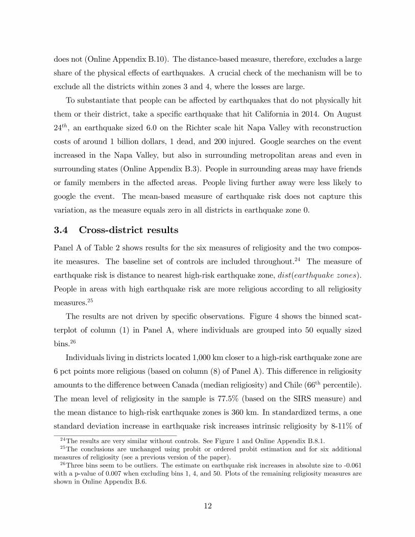
The results are not driven by specific observations. Figure 4 shows the binned scat-

terplot of column (1) in Panel A, where individuals are grouped into 50 equally sized

bins.26

Individuals living in districts located 1,000 km closer to a high-risk earthquake zone are

6 pct points more religious (based on column (8) of Panel A). This difference in religiosity

amounts to the difference between Canada (median religiosity) and Chile (66th percentile).

The mean level of religiosity in the sample is 77.5% (based on the SIRS measure) and

the mean distance to high-risk earthquake zones is 360 km. In standardized terms, a one

standard deviation increase in earthquake risk increases intrinsic religiosity by 8-11% of

24The results are very similar without controls. See Figure 1 and Online Appendix B.8.1.25The conclusions are unchanged using probit or ordered probit estimation and for six additional

measures of religiosity (see a previous version of the paper).26Three bins seem to be outliers. The estimate on earthquake risk increases in absolute size to -0.061

with a p-value of 0.007 when excluding bins 1, 4, and 50. Plots of the remaining religiosity measures areshown in Online Appendix B.6.

12

a standard deviation. This amounts to 80% of the well-established gender difference in

religiosity. (Online Appendix B.5).27

Figure 4. Binned scatterplot of the main result including baseline controls

Notes. The plot shows the regression in column (1) of Panel A of Table 2, binned into 50 bins.

One concern is that the estimated impact is driven by an effect on development:

Earthquakes may affect local development, which may in turn influence religiosity. The

literature is inconclusive about the effect of earthquakes on development and also on the

effect of development on religiosity.28 Furthermore, the main variation in the earthquake

risk measure comes from outside the high-risk zones. Therefore, it seems unlikely that

development effects are driving the result. Nevertheless, I account for development in three

distinct ways. First, districts in high-risk zones are arguably more likely to experience

lower development due to earthquakes. I remove districts located within high-risk zones

3 and 4 from the sample in Panel B. The estimates fall slightly, but are statistically

unchanged. The results therefore do not seem to be driven by the districts that suffer

most direct damage, which is consistent with a psychological explanation.

27Numerous studies have shown that women are more religious than men (see review by Trzebiatowska& Bruce (2012)).28See e.g., Ahlerup (2013) for a positive effect of earthquakes on development, Cavallo et al. (2013) for

a negative impact. The secularization hypothesis does not find much support in the data (e.g.,Inglehart& Baker (2000), Norris & Inglehart (2011), Stark & Finke (2000), and Iannaccone (1998)).

13

Table 2. OLS estimates of Religiosity on Earthquake risk

(1) (2) (3) (4) (5) (6) (7) (8)

Dependent variable: impgod relpers service comfort believe afterlife SRS SIRS

Panel A. Baseline results

Dist(earthquake zones), 1000km -0.052*** -0.044** -0.035** -0.059*** -0.035** -0.115*** -0.062*** -0.063***

(0.014) (0.019) (0.015) (0.020) (0.018) (0.026) (0.016) (0.016)

[0.015] [0.022] [0.018] [0.026] [0.021] [0.028] [0.016] [0.017]

[0.011] [0.016] [0.012] [0.017] [0.015] [0.020] [0.013] [0.013]

Observations 198,264 192,120 196,860 126,195 129,910 120,072 103,282 104,040

R-squared 0.407 0.208 0.278 0.263 0.226 0.202 0.337 0.325

Districts 884 880 868 611 592 592 591 591

Countries 85 84 83 67 66 66 66 66

Panel B. Excluding districts located in earthquake risk zones 3 and 4

Dist(earthquake zones), 1000km -0.039*** -0.041** -0.029* -0.058*** -0.037* -0.106*** -0.055*** -0.058***

(0.014) (0.021) (0.016) (0.022) (0.020) (0.026) (0.017) (0.018)

Observations 167,430 162,276 165,571 103,071 106,076 97,917 84,418 84,975

R-squared 0.408 0.199 0.291 0.268 0.232 0.195 0.340 0.327

Districts 748 744 732 506 488 488 487 487

Panel C. Adding controls for district level development and dummies for individual education

Dist(earthquake zones), 1000km -0.053*** -0.049** -0.036** -0.055*** -0.038** -0.118*** -0.064*** -0.065***

(0.014) (0.020) (0.015) (0.020) (0.018) (0.026) (0.016) (0.017)

Observations 187,770 180,656 185,141 117,021 121,469 112,453 97,033 97,523

R-squared 0.400 0.195 0.276 0.252 0.233 0.211 0.339 0.329

Districts 869 866 854 586 578 578 577 577

Panel D. Adding squared earthquake risk

Dist(earthquake zones), 1000km -0.091*** -0.087*** -0.064** -0.087*** -0.058** -0.166*** -0.083*** -0.088***

(0.023) (0.032) (0.025) (0.034) (0.027) (0.040) (0.025) (0.027)

Dist(earthquake zones) squared 0.023*** 0.025** 0.017** 0.023 0.019 0.041** 0.017 0.020

(0.007) (0.010) (0.008) (0.020) (0.014) (0.017) (0.013) (0.014)

Observations 198,264 192,120 196,860 126,195 129,910 120,072 103,282 104,040

R-squared 0.407 0.208 0.279 0.263 0.226 0.202 0.337 0.325

Impact at 500 km -0.0793 -0.0746 -0.0557 -0.0759 -0.0491 -0.145 -0.0743 -0.0775

Baseline controls Y Y Y Y Y Y Y Y

Notes. The unit of analysis is an individual. The dependent variables are the six measures of religiosity listed in Table 1 and their

composite measures. Dist(earthq zones) measures the distance in 1000 km to the nearest earthquake zone 3 or 4. Baseline controls

are described under equation (1). All columns include a constant. Standard errors are clustered at the subnational district level in

parenthesis, at the country level in the first set of squared brackets, and corrected using Conley’s (1999) correction in the second

set of squared brackets (cutoff = 500 km). Asterisks ***, **, and * indicate significance at the 1, 5, and 10% level, respectively,

based on the standard errors clustered at the district level.

RESULTS: Districts closer to high-risk earthquake zones are more religious, even controlling for actual recent earthquakes and

development. And also when excluding districts within the high-risk earthquake zones.

14

Second, Panel C adds dummies for eight education categories and average lights visible

by night per square km, widely used in recent research as a proxy for local development.29

The impact of earthquake risk on religiosity remains unchanged. These results should

be interpreted with caution, as education and development are potentially endogenous to

religiosity. Third, the result persists after including alternative measures of development,

such as individual-level income deciles, unemployment status, a dummy for whether the

respondent works in agriculture, and population density. Adding more exogenous devel-

opment proxies - share of arable land and soil quality - also does not alter the results

(Online Appendix B.8).

Panel D checks the linearity of the estimate of earthquake risk on religiosity. Even

if the religious coping hypothesis was true, one would not expect that individuals living

2,000 km from a high-risk earthquake zone are more religious than those living 2,100 km

away because of the increased distance. Both of these groups live far from earthquake

zones, and 100 km should not matter. Panel D confirms the diminishing impact of distance

across most religiosity measures.30

3.5 Other natural disasters

Table 3 shows the impact of the risk of four geophysical and metereological disasters on

religiosity: Earthquakes, tsunamis, volcanic eruptions, and tropical storms.31 The mea-

sure of religiosity is the composite measure, SIRS. People are more religious in areas with

high risk of earthquakes or tsunamis, but even more so if the risk of both disasters is high

(columns 1-4). Increased risk of volcanic eruptions also increases religiosity, but only in

districts within 1000 km of a volcanic eruption zone, most likely due to the spatial con-

centration of volcanic eruptions (column 5). The risk of storms does not affect religiosity

(columns 7 and 8). These findings are consistent with the religious coping literature,

where mainly unpredictable disasters instigate a need for religion in coping. Meteorol-

29Education categories run from 1, which indicates "Inadequately completed elementary education" to8, which indicates "University with degree / Higher education". Lights are based on NASA’s pixel levellights data. The wealthier the district and the more educated the individual is, the lower the level ofreligiosity (estimates not shown).30The same conclusion is reached if one excludes districts in increments of 500 km from earthquake

zones (see a previous version of this paper).31These are the worst types of geophysical and meteorological disasters across the globe based on

the map of natural disasters from Munich Re (www.munichre.com). The correlations with distance toearthquake zones are: 0.457 (volcanic eruptions), 0.381 (tsunamis), and 0.196 (storms), respectively. Alldisaster data are described in Online Appendix B.13.

15

ogists have a much easier time predicting storms than seismologists have in predicting

earthquakes.32

Table 3. Main results with alternative disaster measures

Dep var.: SIRS (1) (2) (3) (4) (5) (6) (7) (8)

Disaster: Earthq Tsunami Earthq and Earthq and Volcano Volcano Storm Storm

tsunamis tsunamis

Distance measure: dist dist avg dist min dist dist dist dist

Distance(disasters), 1000 km -0.063*** -0.067*** -0.094*** -0.089*** -0.008 -0.026** -0.014 0.012

(0.016) (0.017) (0.021) (0.019) (0.007) (0.013) (0.014) (0.029)

Observations 104,040 104,040 104,040 104,040 104,040 59,132 104,040 38,643

R-squared 0.325 0.326 0.326 0.326 0.325 0.333 0.325 0.328

Baseline controls Y Y Y Y Y Y Y Y

Sample Full Full Full Full Full <1000 km Full <1000 km

Districts 591 591 591 591 591 321 591 129

Notes. OLS estimates. The dependent variable is the Strength of Intrinsic Religiosity Scale. The disaster measure is distance

to earthquake zones 3 or 4 in column (1), tsunamis in column (2), the average distance to earthquake zones and tsunamis in

column (3), the minimum distance to earthquake zones or tsunamis in column (4), distance to volcanic eruption zones in

columns (5) and (6), and distance to tropical storm zones in columns (7) and (8). The sample is restricted to districts within 1000

km of high risk disaster zones in columns (6) and (8). All disaster data are described in Appendix B.9. All columns include a

constant. Standard errors (in parenthesis) are clustered at the level of subnational districts. Asterisks ***, **, and * indicate

significance at the 1, 5, and 10% level, respectively.

RESULTS: Higher risk of earthquakes, tsunamis, and volcanic eruptions increase religiosity. Storm risk does not.

3.6 Heterogeneity

Higher earthquake risk increases religiosity on all continents, and for Christians, Muslims,

Jews, and Hindus (Online Appendix B.12). Buddhist beliefs are not significantly affected

by earthquake risk in this sample and with the particular religiosity measures.33 Followers

of monotheistic religions or religions with big gods are also no differently affected than

the rest.34 That followers from rather diverse religions all engage in religious coping is

consistent with the literature on religious coping (e.g., Abu-Raiya & Pargament (2015)).

32The US Geological Survey (USGS) notes that earthquakes cannot be predicted(www2.usgs.gov/faq/categories/9830/3278). See also this post about our ability to forecast stormsand their paths, as opposed to our inability to forecast earthquakes: www.tripwire.com/state-of-security/risk-based-security-for-executives/risk-management/hurricanes-earthquakes-prediction-vs-forecasting-in-information-security/33The results for Jews and Buddhists should be interpreted with caution, as there are only 426 and

1,007 respondents of each in the sample.34The concept "Big Gods" (defined by Norenzayan & Shariff (2008)) refers to the omniscient and

omnipotent higher powers that are prevalent across many major religious traditions today.

16

There is also no differential impact of earthquake risk across income - or education groups

(Online Appendix B.15). However, earthquake risk increases religiosity significantly more

for unemployed individuals, even controlling for income. Employment perhaps provides

something in addition to income, such as social networks, that reduce the need for religion

in coping (e.g., Scheve & Stasavage (2006)).

3.7 Further robustness checks

This section summarizes additional robustness checks, detailed in Online Appendix B.

One concern is that earthquakes influence other cultural values, which are driving the

results. The results are robust to adding controls for alternative cultural values such as

trust, manners, independence, hard work, feeling of responsibility, imagination, tolerance

and respect for other people, thrift, determination and perseverance, unselfishness, and

obedience. Another concern is that earthquake risk correlates with other geographic fea-

tures that drive the correlation. The results are robust to adding average temperature,

average and variance of precipitation, ruggedness, elevation, district area, and a dummy

equal to one if the district is located within high risk zones. The results are also robust

to adding 116 ethnicity fixed effects.

The size of the effect of earthquake risk is statistically similar across all measures of

religiosity. The effect on religiosity is driven mainly by the intensive margin (the degree

of believing), and not by the extensive margin (whether or not people believe). This is

consistent with the idea that conversion into religion is harder to influence than religiosity

among existing believers.

A measure of religiosity that might relate more directly to religious coping is prayer

outside religious services.35 Earthquake risk increases prayer outside religious services,

which is consistent with religious coping and cannot be explained by theories that involve

churchgoing.

3.8 Google searches on religion

The results hold using alternative measures of religiosity based on Google searches.36

People in US states with higher earthquake risk google "God", "Jesus", "Pray", and

"Bible" more as a share of their total Google searches (Figure 5 and Online Appendix35Thank you to an anonymous referee for suggesting this measure.36Thanks to an anonymous referee for suggesting this.

17

B.16).37 They are not more likely to search for churches. This is consistent with the

idea that mainly intrinsic religiosity is used in coping and inconsistent with explanations

involving churchgoing. The results are robust to including four region fixed effects and

controls for distance to the ocean, absolute latitude, and GSP per capita.

Figure 5. Earthquake risk and Google searches on God across US states

4 Event studyThis section exploits the time-dimension of the WVS-EVS data to account for district-

level time-invariant unobservables. The same individuals are not followed over time, but

a third of the districts are measured more than once, which makes it possible to construct

a synthetic panel, where the panel dimension is the subnational district and the time

dimension is the year of interview.38 I match this information with earthquake events at

the district level. The main analysis relies on the following equation:

∆religdcw = α + β∆earthquakedcw + λcw + ∆X ′dcwδ + ∆εdcw, (2)

where ∆religdcw = religdcw−religdcw−1 measures the change in district-level religiosity

between interview waves w − 1 and w in district d in country c. Since religiosity is

37I choose the US based on three criteria: It is one of the countries in the world with the largestinternet penetration, it is geographically large, and it has variation in earthquake risk. The particularsearch terms are chosen based on a New York Times article about using Google trends to measuretrends in religiosity (https://www.nytimes.com/2015/09/20/opinion/sunday/seth-stephens-davidowitz-googling-for-god.html).38Restricting the sample in Table 2 to the sample of districts that were surveyed more than once does

not alter the estimates on earthquake risk.

18

not measured annually, w − 1 can indicate a lag of several years.39 ∆earthquakedcw =

earthquakedcw − earthquakedcw−1 measures either the number of earthquakes that hit

between waves or a dummy equal to one if one or more earthquakes hit in between

the waves. Baseline controls include country-by-year fixed effects (λcw), individual-level

controls for sex, marital status, age, and age squared, time-varying district-level controls

for the number of years between interviews and the number of years since an earthquake

hit (∆X ′dcw). Additional controls are added as robustness.40

Equation (3) allows the impact of earthquakes to vary depending on how often the

district is otherwise hit:

∆religdcw = α+ β∆earthqdcw + γ∆earthqdcw · frequentdc +λcw + ∆X ′dcwδ+ ∆εdcw, (3)

where frequentdc is a dummy equal to one if the district is frequently hit by earth-

quakes.

4.1 Data on earthquake events

The Advanced National Seismic System at the US Geological Survey provides data on

the timing, location, and severity of earthquakes since 1898 (Online Appendix C.1). The

analysis exploits the 68,711 earthquakes that hit the surface of the Earth between 1973

and 2014 of magnitude 5 or above.41 Figure 6 shows earthquakes split into those of

magnitude 5-5,999 (dark blue dot) and those of magnitude 6 or above (larger red dot).

I combine the earthquakes with the shapefile of subnational districts used in Section

3.4. I define a district as being hit by an earthquake if the earthquake hit within X km

of the district border. I choose X low enough to ensure that the earthquake was likely to

influence the people in the particular district, but high enough to ensure that potentially

39religdcw is based on information at the individual level aggregated up to the district level, using

appropriate weights (variable s017), sidcw: religdcw = 1N

N∑i=1

sidcw · r̂eligidcw, where r̂eligidcw measures the

residuals of a regression of religidcw on the included individual-level controls.40Standard errors are clustered at the country-level throughout. Conclusions are the same if using

instead unclustered standard errors.41Due to improvements in earthquake-detection technology, earthquakes of magnitudes below 5 on

the Richter Scale cannot be compared over time, and neither can earthquakes of any size before 1973.The number of earthquakes of all magnitudes in the data increases up until 1973 and the number ofearthquakes of magnitudes below 5 increases over the entire period. Since the number of earthquakeshas not increased in reality, the implication is that earthquake detection technology must have improvedover time. There has been no trend in the number of earthquakes of magnitude 5 or above since 1973.

19

influential earthquakes are not lost. For the main analysis, a district is defined as having

been hit when an earthquake hit within 100 km of the district border. The results are

robust to alternative cut-offs (Online Appendix C.2).

As expected, larger earthquakes increase religiosity more (Online Appendix C.10). For

the main analysis, I use earthquakes of magnitude 6 or above (the red dots in Figure 6).42

The dummy, frequentdc, equals one for districts frequently hit by earthquakes, zero

otherwise. I define frequently hit as being hit by a total of 7 or more earthquakes over the

period 1973-2014, where 7 is the 95th percentile in the distribution of earthquakes. There

are 13 such districts in the sample. The results are robust to similar definitions of being

frequently hit (Online Appendix C.6).

I drop 38 observations where an earthquake hit in the same year as the WVS-EVS

interview, as it is not possible to identify whether the earthquake hit before or after the

interview for these observations.43 Dropping the 38 observations also means dropping the

districts that are most often hit by earthquakes, including districts where earthquakes hit

within district borders. The main results therefore exclude districts that are directly hit

by earthquakes, i.e. where the earthquake hit within zero km of the district borders. This

helps in disentangling the psychological effect from potential economic effects.

42Earthquake zones 3-4 (used in Section 3.4) correspond to earthquakes with magnitudes above 6.0 onthe Richter scale. As the cross-district analysis uses the distance to these zones, it implicitly also includesthe smaller earthquakes. The earthquakes in the event study are measured in terms of magnitude, whichincludes the Richter Scale, but also other comparable scales.43The WVS-EVS provides information on the year of interview for all respondents. Information on the

month of the interview is available for a third of the sample. Hence, if distance to the nearest earthquakein each month was calculated, a maximum of 12 observations could be gained (a third times the 38observations), provided that none of the earthquakes hit in the same month as the interview. However,there may be a selection bias when comparing these districts with those with only yearly information.The results are robust to including the particular observations.

20

Figure 6. Epicentres of earthquakes of magnitude 5 or above on the Richter scale, 1973-2014

Source: The US Geological Survey.

4.2 Data on religiosity

The event study suffers from having few observations, since only a third of the districts

are measured more than once. The three questions on religiosity available for most re-

spondents are "How important is God in your life?", "Are you a religious person?", and

"How often do you attend religious services?" These are available for 250 districts located

in more than 30 countries. The remaining three measures of religiosity (beliefs in God,

finding comfort in God, and beliefs in an Afterlife) are available for only half the number

of districts in half the number of countries. Earthquakes do not affect these remaining

measures of religiosity statistically in the present data (Online Appendix C.11).44

The panel is unbalanced. Some districts are interviewed in two consecutive years and

others are interviewed with a gap of 18 years. The average is 5 years (Online Appendix

C.7). In order not to loose important short-term effects, the main sample is restricted to

districts measured with a gap of 10 years or less. The unbalancedness of the sample does

not seem to influence results (Online Appendix C.7). The results are robust to different

cut-offs and to estimating the levels-regressions of the district-aggregate of equation (2)

with district fixed effects.45

44Insignificance may reflect that these three measures capture conversion rates, which are affected lessthan the degree of believing. Insignificance is not due to the smaller sample: Earthquakes continue toincrease average importance of God and the share of religious persons in the smaller sample (OnlineAppendix C.11).45Thanks to an anonymous referee for suggesting this.

21

4.3 Results

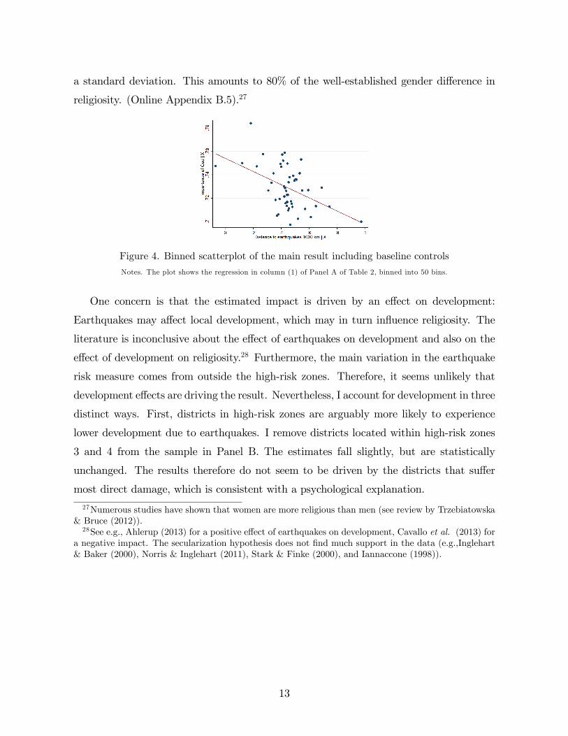
According to the religious coping hypothesis, adversity is expected to increase intrinsic

religiosity, i.e. personal beliefs and private prayer. And not necessarily churchgoing.

Figure 7 shows the average change in the two measures of intrinsic religiosity. Average

importance of God fell by 0.2 pct points in the 327 district-years that were not hit by

earthquakes compared to an increase of 1.8 pct points in the 39 district-years that were

hit. The increase was more than double as large (4.0 pct points) in the 22 district-years

that were hit, but where earthquakes are otherwise rare. The difference between the

blue and red dot has a p-value of 0.08. The share of religious persons has fallen in all

three samples, but only significantly in districts that were not hit by earthquakes. The

difference between the blue and red dot has a p-value of 0.71. The degree of believing is

more easily affected by adversity, while conversion rates are more persistent. Restricting

the sample to districts measured with a gap of 6 years or less reduces the p-values of

the difference between red and blue dots to 0.03 and 0.18, respectively (Online Appendix

C.3).

Figure 7. Average change in religiosity by earthquake or not

Notes. Lines show the 90 pct confidence bounds.

Next, I turn to more formal econometric analysis. Table 4 shows the results from

estimating equation (2) and (3) for the three religiosity measures and the two measures

of earthquake events. Baseline controls are included throughout and eight education

dummies are added in even columns.46 Earthquakes increase intrinsic religiosity, while

churchgoing is unaffected (Panel A). These results are consistent with religious coping,

but inconsistent with theories involving churchgoing. One concern is that churchgoing is

46The main results are qualitatively robust to estimating without controls (Online Appendix C.4).

22

insignificant because the sample is different from the other religiosity measures or because

of the specific categorization of the variable. This concern does not seem to be borne out

in the data: Churchgoing remains insignificant in different samples and with different

categorizations (Online Appendix C.5.2 and C.11.1).

Earthquakes in districts that are otherwise rarely hit increase religiosity more than

earthquakes in districts that are often hit (Panel B).47 In fact, earthquakes in frequently

hit districts do not increase religiosity.

One concern is that district-level trends correlate with earthquakes and the change in

religiosity, which could be driving the results. The placebo test in Panel C addresses this

concern by showing that future earthquakes have no effect on current religiosity.48

Average religiosity increases by 7.6 pct points in districts hit by one or more earth-

quakes, compared to districts that did not experience any earthquakes (based on column

(1) in Panel A). This corresponds to increasing religiosity from the median district to the

80th percentile (in terms of changes in religiosity). A one standard deviation increase in

the probability of being hit by an earthquake increases intrinsic religiosity by 23-28% of

a standard deviation, depending on whether the district is frequently hit by earthquakes

or not. Conversion rates increase by 11-13% of a standard deviation (Online Appendix

C.5.1).

47This finding is not driven by higher religiosity in high-risk districts: The finding is robust to addinginitial religiosity and its’interaction with earthquakes (Online Appendix C.12.1).48Current earthquakes continue to increase religiosity when added together with future earthquakes

(Online Appendix C.9). Future earthquakes continue to have no effect on religiosity.

23

Table 4. OLS estimates of the change in religiosity on earthquakes

(1) (2) (3) (4) (5) (6) (7) (8) (9) (10) (11) (12)

Dependent variable ∆impgod ∆relpers ∆service ∆impgod ∆relpers ∆service

Earthquake measure: Earthquake dummy Number earthquakes

Panel A. Baseline results

Earthquake measure 0.076*** 0.074*** 0.053** 0.046** 0.034 0.031 0.027** 0.024*** 0.022*** 0.020*** 0.015 0.014

(0.023) (0.021) (0.021) (0.019) (0.030) (0.037) (0.010) (0.008) (0.007) (0.006) (0.009) (0.010)

R-squared 0.335 0.314 0.414 0.413 0.509 0.507 0.325 0.304 0.413 0.412 0.508 0.506

Panel B. Allowing the impact of earthquakes to vary with how frequently a district is hit

Earthquake measure 0.093*** 0.086*** 0.062** 0.060** 0.024 0.018 0.058** 0.053** 0.044*** 0.043*** 0.017 0.016

(0.028) (0.023) (0.027) (0.023) (0.044) (0.052) (0.021) (0.020) (0.014) (0.012) (0.022) (0.025)

Earthquake x Frequent earthquake -0.073** -0.060* -0.058 -0.063* 0.014 0.046 -0.053*** -0.048** -0.046** -0.044*** -0.018 -0.017

(0.029) (0.031) (0.041) (0.033) (0.077) (0.090) (0.019) (0.019) (0.018) (0.014) (0.025) (0.029)

R-squared 0.338 0.316 0.417 0.415 0.513 0.513 0.333 0.311 0.417 0.415 0.513 0.512

Panel C. Placebo regressions

Earthquake measure w+1 -0.027 -0.017 0.023 0.027 -0.064 -0.057 -0.025 -0.017 0.007 0.012 -0.050 -0.040

(0.021) (0.026) (0.041) (0.046) (0.047) (0.044) (0.018) (0.021) (0.031) (0.033) (0.034) (0.033)

Earthquake w+1 x Frequent earthquake -0.015 -0.031 -0.005 -0.016 0.110* 0.120** 0.016 0.009 -0.007 -0.010 0.037 0.031

(0.021) (0.028) (0.046) (0.052) (0.062) (0.056) (0.017) (0.021) (0.029) (0.032) (0.034) (0.033)

R-squared 0.320 0.299 0.414 0.413 0.518 0.516 0.320 0.299 0.414 0.412 0.517 0.514

Observations 350 324 370 333 384 347 350 324 370 333 384 347

Baseline controls Y Y Y Y Y Y Y Y Y Y Y Y

Eight education dummies N Y N Y N Y N Y N Y N Y

Districts 236 230 250 240 264 254 236 230 250 240 264 254

Countries 31 30 31 30 32 31 31 30 31 30 32 31

Number Fixed effects 46 50 47 49 48 50 46 50 47 49 48 50

Notes. The unit of analysis is districts. The dependent variable is the change in average importance of God in col (1)-(2) and (7)-(8), the change in share of religious persons in

col (3)-(4) and (9-10), and the change in average churchgoing in col (5)-(6) and (11)-(12). The earthquake measure is a dummy equal to one if one or more earthquakes hit the

district in between interviews, zero otherwise (col 1-6) and the number of earthquakes (col 7-12). All columns include a constant. Standard errors (in parenthesis) are clustered

at the country level. Asterisks ***, **, and * indicate significance at the 1, 5, and 10% level, respectively.

RESULTS: Earthquakes increase intrinsic religiosity and not churchgoing. The effect is larger in districts that are rarely hit. Future earthquakes do not affect current religiosity.

24

4.4 Heterogeneity

Earthquakes increase religiosity across all major denominations and continents, for indi-

viduals with different levels of initial religiosity and from all income and education groups

(Online Appendices C.12 and C.13). Religiosity rises more in districts with lower aver-

age incomes, education levels, or population densities, but there is no difference across

different levels of light density or unemployment rates.

4.5 Further robustness checks

This section summarizes further robustness checks detailed in Online Appendix C.

The results are robust to adding additional controls for initial religiosity, ethnic fixed

effects, income fixed effects, the same list of alternative cultural values as in Section 3.4,

religious denomination fixed effects, a year trend, and lagged earthquakes.

Consistent with existing studies on cultural values (e.g., Perrin & Smolek (2009) and

Dinesen & Jæger (2013)), the impact of earthquakes on religiosity abates after a while.

The impact on religiosity lasts up to 9-12 years, while the impact on conversion rates lasts

3 years. Churchgoing is not affected in any of the time windows, but this study cannot

rule out that churchgoing could be affected in time windows shorter than 3 years.

One concern when differentiating with respect to the frequency at which a district

is hit is that frequently hit districts with earthquakes are compared to districts without

earthquakes and districts hit by an earthquake, but otherwise rarely hit. To tighten the

comparison group, I restrict the sample to districts hit by at least one earthquake. Results

are unchanged.

4.6 Event study vs cross-district results

One way to reconcile the results from the cross-district analysis and the event study is

to regard the former as documenting long-term effects and the latter as documenting

short-term effects. The short-term effect of earthquakes on importance of God is more

than double the size of the long-term effect.49 This difference is likely due to dynamics:

While the short-term effect abates after a while, the long-term results indicate that a

residual may survive, adding up to significant long-term differences. Another reason

49This calculation is based on dividing the standardized coeffi cient in column (1) of Table A32 withthat in column (1) of Table A7: |betaearth|

|betadist(earthq)| =0.2260.082 = 2.756

25

for the difference in the size of the effect could be that the risk measure is based on the

continuous distance to high-risk zones and thus also includes smaller earthquakes. Indeed,

the long-term effect is 30% larger for districts within 100 km of high-risk zones, compared

to the full sample.

While only intrinsic religiosity is affected in the short term, both extrinsic and intrinsic

religiosity are affected in the long term. If anything, it seems that as people become more

religious, they go more to church. Not the other way around. Buddhist beliefs increase

in the aftermath of earthquakes, but this effect vanishes in the long term: Buddhists in

high-risk areas are not more religious than Buddhists in low-risk areas. Perhaps Buddhist

beliefs are more effi cient in providing stress relief than other beliefs, thus reducing the

need for religion in the long term.

An earthquake in poorer districts is more likely to increase average religiosity, com-

pared to one in richer districts. This differential effect seems to vanish over time: Increased

earthquake risk is equally likely to increase religiosity in poor and rich districts. The im-

plicit inclusion of small earthquakes in the risk measure could explain this difference

between results. But the different results may also be due to transmission of religiosity

across space or generations. The latter is investigated below.

5 Epidemiological approachThe religious coping hypothesis concerns the immediate effect on religiosity from adverse

life events, and is silent on transmission across generations. Whether religiosity is passed

on through generations can be investigated in a model of cultural transmission (Bisin

& Verdier (2001)). Parents transmit a particular cultural trait to their children if this

grants utility to parents or children. Studies find that religious individuals often have

better mental health (Miller et al. (2014), Park et al. (1990)), higher life satisfaction

(Ellison et al. (1989), Campante & Yanagizawa-Drott (2015)), are better able to cope

with adverse life events (Clark & Lelkes (2005)), and engage less in deviant behavior

(Lehrer (2004)).50 Thus, religion might have some benefits that parents would like to

transmit to their children.51

50See also reviews by Smith et al. (2000) and Pargament (2001).51Another way to think of the transmission of religiosity is that people who believe in God will pass

this "worldview" on to their children like any other knowledge of the World. People who do not believein God will also pass on this disbelief.

26

This section investigates whether second generation immigrants are more religious

when their parents came from a country with higher earthquake risk, compared to those

with parents from lower earthquake risk areas. The method is also called the epidemio-

logical approach (e.g., Fernandez (2011)). I estimate the following equation:52

religiositycjat = α + βearthquakea + rct +X ′cjatη +W ′aδ + V ′jatλ+ εcjat,

where religiositycjat is the religiosity level of individual j interviewed at time t living

in country c in which he/she was born, and with parents who migrated from country a.

earthquakea is earthquake risk in the country of origin, as described in Section 3.4. rct is

country of residence by year fixed effects. This removes any country-level factors in the

individual’s current environment, such as institutions, earthquake frequency, and average

religiosity. Xcjt is a vector of individual-level controls. Wa are factors in the parents’

country of origin that are likely to correlate with earthquake risk and religiosity. Vjat is a

vector of socioeconomic characteristics of the parents.

I use the European Social Survey (ESS), which includes five survey rounds over the

period 2004-2012 for 17,587 individuals whose parents were born in 171 different coun-

tries.53 The surveys include three questions on religiosity: (1) How often do you pray

apart from at religious services? (1="Never", ..., 7="Every day"), (2) How religious are

you? (1="Not at all religious", ..., 10="Very religious"), and (3) How often do you at-

tend religious services apart from special occasions? (1="Never", ..., 6="More than once

a week").54 I rescaled the variables to lie between 0 and 1. In cases where the parents

migrated from different countries, I use the mothers’country of origin.55

Individuals whose parents came from a country with high earthquake risk pray more

often, regard themselves as more religious, and attend religious services more often than

those whose parents came from less earthquake prone countries (Panel A, Table 5). The

52The equation is estimated by OLS, but results are robust to using instead ordered logit estimation.53The ESS is available at www.europeansocialsurvey.org. Another dataset with information on the

religiosity of second generation immigrants is the General Social Survey (GSS) conducted in the UnitedStates. However, the respondents only come 30 countries and two aggregated regions, compared to 171countries in the ESS.54The frequency of attending religious services was originally a variable running from 1="Never" to

7="Every day". Due to few observations in the latter category, I merged 7 and 6="More than once aweek". The results are unchanged if using the original variable (Online Appendix Table A60).55Results are robust to focusing on the fathers’country of origin (Online Appendix Table A61).

27

result is robust to adding controls for absolute latitude, continent dummies, and dis-

tance to the coast in the parents’country of origin (columns 2, 5, and 8) and to adding

individual-level characteristics (age, age squared, sex, and the five education fixed effects)

and five fixed effects for parents’education (columns 3, 6, and 9).

Corroborating the cross-district results in Table 2, the impact of earthquake risk is

unchanged when restricting to individuals whose parents came from countries not directly

located in high-risk earthquake zones (Panel B). Again, the impact of distance diminishes

with distance (Panel C).

The results in Table 5 are consistent with the idea that high earthquake risk instigates

a culture of high religiosity which is passed on through generations. People who have never

themselves experienced an earthquake can still be influenced by the disasters experienced

by earlier generations, in terms of increased religiosity.

Additional robustness checks are detailed in Online Appendix D, summarized here.

The results are robust to adding a dummy for whether the respondent belongs to an ethnic

minority, denomination fixed effects, ten income fixed effects, and to adding additional

country-of-origin controls (pct Muslims, Christians, Jews, Buddhists, and Hindus, real

GDP per capita, and measures of democracy and property rights). The results for prayer

are robust to different categorizations of the variable. The results for religious person and

churchgoing are not robust, which supports the results in the remainder of the paper. The

exercise in Table 5 implicitly assumes that higher earthquake risk increases religiosity in

the country of origin, and next that this higher religiosity is transmitted across genera-

tions. Consistent with this idea, I find that religiosity in the parents’country of origin

increases their childrens’religiosity. Last, one could expect some bias arising from the

fact that the analysis in this section ignores variation within country of origin. This bias

does not seem to be large.

28

Table 5. OLS estimates of religiosity on earthquake risk in parents’home country

(1) (2) (3) (4) (5) (6) (7) (8) (9)

Dependent variable: pray pray pray religious religious religious service service service

Panel A. Simple linear effect

Dist(earthq zones), -0.050*** -0.036*** -0.028** -0.054*** -0.039*** -0.031** -0.041*** -0.027** -0.021**

1000 km (0.014) (0.011) (0.011) (0.017) (0.014) (0.013) (0.014) (0.011) (0.010)

Observations 17,155 17,058 14,156 17,271 17,174 14,250 17,334 17,236 14,304

R-squared 0.122 0.129 0.175 0.074 0.085 0.129 0.100 0.110 0.127

Org countries 171 166 155 171 166 155 171 166 155

Panel B. Excluding countries of origin in high-risk zones

Dist(earthq zones), -0.044*** -0.038*** -0.026** -0.047*** -0.039*** -0.030** -0.036*** -0.027** -0.018**

1000 km (0.015) (0.011) (0.011) (0.017) (0.013) (0.014) (0.012) (0.010) (0.009)

Observations 15,787 15,784 9,367 15,894 15,891 9,407 15,957 15,954 9,435

R-squared 0.105 0.112 0.159 0.062 0.072 0.122 0.094 0.102 0.127

Org countries 139 136 123 139 136 122 139 136 123

Panel C. Including squared earthquake risk

Dist(earthq zones), -0.130*** -0.079*** -0.068** -0.121*** -0.059** -0.048* -0.090*** -0.042** -0.033

1000 km (0.021) (0.024) (0.027) (0.027) (0.026) (0.027) (0.027) (0.019) (0.021)

Dist(earthq zones) 0.049*** 0.024* 0.023 0.041*** 0.011 0.010 0.029** 0.009 0.007

squared (0.010) (0.014) (0.017) (0.013) (0.014) (0.017) (0.012) (0.010) (0.008)

Observations 17,155 17,058 14,156 17,271 17,174 14,250 17,334 17,236 14,304

R-squared 0.123 0.130 0.175 0.075 0.085 0.129 0.101 0.110 0.127

Impact at 500 km -0.105 -0.0666 -0.0566 -0.101 -0.0532 -0.0432 -0.0749 -0.0377 -0.0293

Country-year FE Y Y Y Y Y Y Y Y Y

Geo controls N Y Y N Y Y N Y Y

Parent and respondent

controls N N Y N N Y N N Y

Notes. The unit of analysis is a second generation immigrant. The dependent variable is answers to the question: "How often do

you pray apart from at religious services?" in col (1)-(3), "How religious are you?" in col (4)-(6), and "How often do you attend

religious services apart from special occations?" in col (7)-(9). Dist(earthq zones) measures distance to the nearest high risk

earthquake zone. "Geo controls" indicates country of origin controls for continent dummies (Africa, Asia, Australia and Oceania,

Europe, North America, and South America), absolute latitude, and distance to the coast. "Parent and respondent controls"

indicates five education fixed effects for parents and respondent, and controls for the respondent’s age, age squared, and sex.

Standard errors (in parenthesis) are two-way clustered at the country of residence and parents’country of origin. Asterisks ***, **,

and * indicate significance at the 1, 5, and 10% level, respectively.

RESULTS: Second generation immigrants from countries with higher earthquake risk are more religious than their peers living in

the same country, but whose parents came from countries with lower earthquake risk.

29

6 ConclusionExploiting natural disasters as a determinant of random and adverse life events, I find that

individuals across the globe become more religious when hit by earthquakes. Particularly

individuals in districts that are otherwise rarely hit. The effect of any earthquake lasts

3-12 years, but a residual impact remains and is transmitted across generations. The main

results are based on global surveys, but similar patterns emerge for alternative measures

of religiosity based on Google searches: People google religious terms more as a share of

their total searches in US states with higher earthquake risk, compared to states with

lower risk of earthquakes.

The results across all three analyses are consistent with religious coping, which involves

using religion psychologically to cope with unbearable and unpredictable events. This

conclusion is based on three main checks. First, if the mechanism is psychological, people

do not have to be hit directly by the earthquake in order to use religion for stress relief. The

data corroborate this idea: Religiosity increases after an earthquake has hit a neighbouring

district. Likewise, long-term religiosity is higher in districts neighbouring the high-risk

districts, compared to districts further away. This indicates that individuals might use

religion to cope with the distress caused by earthquakes that hit friends or family members

in neighbouring districts.

Second, the literature on religious coping agrees that people are more likely to use

religion to cope with unpredictable events, compared to predictable ones (where people

use problem-focused coping to a larger extent). In accordance with this, I find that

only surprising disasters (earthquakes, tsunamis, and volcanic eruptions) and surprising

earthquakes (in districts otherwise rarely hit) increase religiosity. Unsurprising disasters

(tropical storms) and unsurprising earthquakes (in districts frequently hit) do not. The

third check used to investigate whether results are consistent with religious coping is based

on the idea from the religious coping literature that people use their intrinsic religiosity

to cope with adversity to a larger extent than churchgoing. The event study and the

study using Google searches corroborate this idea: Only intrinsic religiosity increases in

response to earthquakes, while churchgoing is unchanged. The estimate on churchgoing

in the cross-district analysis is smaller than the estimate on intrinsic religiosity, but not

statistically.

30

Some of the results are also consistent with alternative explanations. For instance, the

results in the event study are also consistent with the idea that certain types of people

move in and out of districts before and after earthquakes, perhaps as aid workers. But

only religious coping can explain all results across all analyses.

Earthquakes increase religiosity across the major religious denominations, confirming

the idea by early scholars such as Karl Marx and Sigmund Freud, that all religions provide

a psychological coping mechanism. This rules out a distinct theological channel. Likewise,

people from all income and education groups are likely to respond to earthquakes with

increased religiosity. It seems these people have similar psychological needs, despite their

different economic needs.

The empirical analyses overall point to a core psychological explanation of religion.

Religious coping provides a stable reason for why people believe in God. Coping, therefore,

may be one reason why religion has not vanished as some scholars have theorized.

ReferencesAbu-Raiya, Hisham, & Pargament, Kenneth I. 2015. Religious coping among diversereligions: Commonalities and divergences. Psychology of Religion and Spirituality,7(1), 24.

Ager, P., Hansen, C. W., & Loenstrup, L. 2016. Church Membership and Social Insurance:Evidence from the Great Mississippi Flood of 1927. University of Southern DenmarkDiscussion Papers on Business and Economics, 7.

Ager, Philipp, & Ciccone, Antonio. 2018. Agricultural risk and the spread of religiouscommunities. Journal of the European Economic Association, 16(4), 1021—1068.

Ahlerup, Pelle. 2013. Are Natural Disasters Good for Economic Growth? Univeristy ofGothenburg Working Paper, 553.

Alesina, A.F., Giuliano, P., & Nunn, N. 2013. On the origins of gender roles: Women andthe plough. Quarterly journal of Economics, 128(2), 469—530.

Altonji, Joseph G, Elder, Todd E, & Taber, Christopher R. 2005. Selection on observedand unobserved variables: Assessing the effectiveness of Catholic schools. Journal ofpolitical economy, 113(1), 151—184.

Andersen, Thomas Barnebeck, Bentzen, Jeanet, Dalgaard, Carl-Johan, & Sharp, Paul.2017. Pre-reformation Roots of the Protestant Ethic. The Economic Journal, 127(604),1756—1793.

31

Ano, Gene G, &Vasconcelles, Erin B. 2005. Religious coping and psychological adjustmentto stress: A meta-analysis. Journal of clinical psychology, 61(4), 461—480.

Becker, S.O., & Woessmann, L. 2009. Was Weber wrong? A human capital theory ofProtestant economic history. The Quarterly Journal of Economics, 124(2), 531—596.

Belloc, Marianna, Drago, Francesco, & Galbiati, Roberto. 2016. Earthquakes, Religion,and Transition to Self-Government in Italian Cities. The Quarterly Journal of Eco-nomics, 131(4), 1875—1926.

Bentzen, Jeanet Sinding. 2013. Origins of religiousness: The role of natural disasters.Univ. of Copenhagen Dept. of Economics Discussion Paper.

Binzel, Christine, & Carvalho, Jean-Paul. 2017. Education, social mobility and religiousmovements: The Islamic revival in Egypt. The Economic Journal, 127(607), 2553—2580.

Bisin, Alberto, & Verdier, Thierry. 2001. The economics of cultural transmission and thedynamics of preferences. Journal of Economic theory, 97(2), 298—319.

Bjorck, Jeffrey P, & Cohen, Lawrence H. 1993. Coping with threats, losses, and challenges.Journal of Social and Clinical Psychology, 12(1), 56—72.

Buggle, Johannes Christoph, & Durante, Ruben. 2017. Climate risk, cooperation, andthe co-evolution of culture and institutions. CEPR Discussion Paper DP12380.

Buser, Thomas. 2015. The effect of income on religiousness. American Economic Journal:Applied Economics, 7(3), 178—95.

Campante, Filipe, & Yanagizawa-Drott, David. 2015. Does religion affect economic growthand happiness? Evidence from Ramadan. The Quarterly Journal of Economics, 130(2),615—658.

Cantoni, Davide. 2015. The economic effects of the Protestant Reformation: testing theWeber hypothesis in the German lands. Journal of the European Economic Association,13(4), 561—598.

Carl Pieper, DPH, Meador, Keith G, & Sheip, Frank. 1992. Religious coping and depres-sion among elderly, hospitalized medically ill men. American Journal of Psychiatry,1(49), 1—2.

Cavallo, Eduardo, Galiani, Sebastian, Noy, Ilan, & Pantano, Juan. 2013. Catastrophicnatural disasters and economic growth. Review of Economics and Statistics, 95(5),1549—1561.

Chen, Daniel L. 2010. Club Goods and Group Identity: Evidence from Islamic Resurgenceduring the Indonesian Financial Crisis. Journal of Political Economy, 118(2), 300—354.

32

Clark, Andrew, & Lelkes, Orsolya. 2005. Deliver us from evil: religion as insurance.Papers on Economics of Religion, 603, 1—36.

Clark, Walter Houston. 1958. How do social scientists define religion? The Journal ofSocial Psychology, 47(1), 143—147.

Cohen, S., & Wills, T.A. 1985. Stress, social support, and the buffering hypothesis.Psychological bulletin, 98(2), 310—357.

Conway, K. 1985. Coping with the stress of medical problems among black and whiteelderly. The International Journal of Aging and Human Development, 21(1), 39—48.

Dehejia, Rajeev, DeLeire, Thomas, & Luttmer, Erzo FP. 2007. Insuring consumptionand happiness through religious organizations. Journal of Public Economics, 91(1),259—279.

Dinesen, Peter Thisted, & Jæger, Mads Meier. 2013. The effect of terror on institutionaltrust: New evidence from the 3/11 Madrid terrorist attack. Political Psychology, 34(6),917—926.

Ellison, Christopher G, Gay, David A, & Glass, Thomas A. 1989. Does religious commit-ment contribute to individual life satisfaction? Social Forces, 68(1), 100—123.

Fernandez, R. 2011. Does culture matter? The Netherlands: North-Holland.

Feuerbach, Ludwig. 1957. The essence of Christianity. Barnes & Noble Publishing.

Fisker, Peter Simonsen. 2012. Earthquakes and economic growth. Development ResearchWorking Paper Series 01/2012.

Freud, Sigmund. 1927. The future of an illusion. Broadview Press.

Galor, Oded, & Özak, Ömer. 2016. The Agricultural Origins of Time Preference. Amer-ican Economic Review, 3064.

Greif, Avner. 1994. Cultural beliefs and the organization of society: A historical and theo-retical reflection on collectivist and individualist societies. Journal of political economy,912—950.

Gruber, Jonathan, & Hungerman, Daniel M. 2008. The Church Versus the Mall: WhatHappens When Religion Faces Increased Secular Competition? The Quarterly journalof economics, 123(2), 831—862.

Guiso, L., Sapienza, P., & Zingales, L. 2003. People’s opium? Religion and economicattitudes. Journal of Monetary Economics, 50(1), 225—282.

Gurin, Gerald, Veroff, Joseph, & Feld, Sheila. 1960. Americans view their mental health:A nationwide interview survey. New York: Basic Books.

33

Hall, D.D. 1990. Worlds of wonder, days of judgment: Popular religious belief in earlyNew England. Harvard University Press.

Iannaccone, Laurence R. 1998. Introduction to the Economics of Religion. Journal ofeconomic literature, 36(3), 1465—1495.

Inglehart, R., & Baker, W.E. 2000. Modernization, cultural change, and the persistenceof traditional values. American sociological review, 19—51.

Inglehart, R., & Norris, P. 2003. Rising tide: Gender equality and cultural change aroundthe world. Cambridge University Press.

Iyer, Sriya. 2016. The new economics of religion. Journal of Economic Literature, 54(2),395—441.

Johnson, Sarah C, & Spilka, Bernard. 1991. Coping with breast cancer: The roles ofclergy and faith. Journal of Religion and Health, 30(1), 21—33.

Kimball, Miles S, Mitchell, Colter M, Thornton, Arland D, & Young-Demarco, Linda C.2009. Empirics on the origins of preferences: The case of college major and religiosity.National Bureau of Economic Research w15182.

Koenig, Harold G, George, Linda K, & Peterson, Bercedis L. 1998. Religiosity and re-mission of depression in medically ill older patients. American Journal of Psychiatry,155(4), 536—542.

Koenig, H.G., George, L.K., & Siegler, I.C. 1988. The use of religion and other emotion-regulating coping strategies among older adults. The Gerontologist, 28(3), 303—310.

Lazarus, R.S., & Folkman, S. 1984. Stress, appraisal, and coping. Springer PublishingCompany.

Lehrer, Evelyn L. 2004. Religion as a determinant of economic and demographic behaviorin the United States. Population and development review, 30(4), 707—726.

Marx, Karl. 1867. Capital: A critique of political economy. The Penguin Group.

Mattlin, Jay A, Wethington, Elaine, & Kessler, Ronald C. 1990. Situational determinantsof coping and coping effectiveness. Journal of Health and Social Behavior, 103—122.

McCleary, R.M., & Barro, R.J. 2006. Religion and economy. The Journal of EconomicPerspectives, 20(2), 49—72.

Miller, Lisa, Bansal, Ravi, Wickramaratne, Priya, Hao, Xuejun, Tenke, Craig E, Weiss-man, Myrna M, & Peterson, Bradley S. 2014. Neuroanatomical correlates of religiosityand spirituality: A study in adults at high and low familial risk for depression. JAMApsychiatry, 71(2), 128—135.

Norenzayan, A., & Hansen, I.G. 2006. Belief in supernatural agents in the face of death.Personality and Social Psychology Bulletin, 32(2), 174—187.

34

Norenzayan, A., & Shariff, A.F. 2008. The origin and evolution of religious prosociality.Science, 322(5898), 58—62.

Norris, Pippa, & Inglehart, Ronald. 2011. Sacred and secular: Religion and politicsworldwide. Cambridge University Press.

Nunn, N., & Wantchekon, L. 2011. The Slave Trade and the Origins of Mistrust in Africa.American Economic Review, 101(7).

Nunn, Nathan, & Puga, Diego. 2012. Ruggedness: The blessing of bad geography inAfrica. Review of Economics and Statistics, 94(1), 20—36.

Ono, K. 1987. Superstitious behavior in humans. Journal of the Experimental Analysisof Behavior, 47(3), 261.

Pargament, K.I. 2001. The psychology of religion and coping: Theory, research, practice.Guilford Press.

Park, C., Cohen, L.H., & Herb, L. 1990. Intrinsic religiousness and religious coping as lifestress moderators for Catholics versus Protestants. Journal of personality and socialpsychology, 59(3), 562.

Penick, J.L. 1981. The New Madrid Earthquakes. University of Missouri.

Perrin, Andrew J, & Smolek, Sondra J. 2009. Who trusts? Race, gender, and the Sep-tember 11 rally effect among young adults. Social science research, 38(1), 134—145.

Ray, Gene. 2004. Reading the Lisbon earthquake: Adorno, Lyotard, and the contemporarysublime. The Yale Journal of Criticism, 17(1), 1—18.

Scheve, K., & Stasavage, D. 2006. Religion and preferences for social insurance. QuarterlyJournal of Political Science, 1(3), 255—286.

Schuster, M.A., Stein, B.D., Jaycox, L.H., Collins, R.L., Marshall, G.N., Elliott, M.N.,Zhou, A.J., Kanouse, D.E., Morrison, J.L., & Berry, S.H. 2001. A national survey ofstress reactions after the September 11, 2001, terrorist attacks. New England Journalof Medicine, 345(20), 1507—1512.

Sibley, Chris G, & Bulbulia, Joseph. 2012. Faith after an earthquake: A longitudinal studyof religion and perceived health before and after the 2011 Christchurch New Zealandearthquake. PloS one, 7(12), e49648.

Siebert, L., & Simkin, T. 2002. Volcanoes of the world: An illustrated catalog of Holocenevolcanoes and their eruptions. Smithsonian Institution, Global Volcanism Program,Digital Information Series GVP-3 (http://www. volcano. si. edu/world).

Skinner, B.F. 1948. ’Superstition’in the pigeon. Journal of experimental psychology, 38(2),168.

35

Smith, Bruce W, Pargament, Kenneth I, Brant, Curtis, & Oliver, Joan M. 2000. Noahrevisited: Religious coping by church members and the impact of the 1993 Midwestflood. Journal of Community Psychology, 28(2), 169—186.

Sosis, R. 2008. Pigeons, foxholes, and the book of Psalms. In: Bulbulia, J, Sosis R. HarrisE. Genet R. Genet C., & Wyman, K. (eds), Evolution of Religion: Studies, Theories,and Critiques. Collins Foundation Press.

Sosis, Richard, & Handwerker, W Penn. 2011. Psalms and coping with uncertainty:Religious Israeli women’s responses to the 2006 LebanonWar. American Anthropologist,113(1), 40—55.

Stark, Rodney, & Finke, Roger. 2000. Acts of faith: Explaining the human side of religion.Univ of California Press.

Trzebiatowska, Marta, & Bruce, Steve. 2012. Why are women more religious than men?Oxford University Press.

Van De Wetering, M. 1982. Moralizing in Puritan natural science: Mysteriousness inearthquake sermons. Journal of the History of Ideas, 417—438.

Voigtländer, Nico, & Voth, Hans-Joachim. 2012. Persecution perpetuated: the medievalorigins of anti-Semitic violence in Nazi Germany. Quarterly Journal of Economics,127(3), 1339—1392.

Weber, M. 1930. trans. Talcott Parsons. The Protestant Ethic and the Spirit of Capitalism.

Williams, D.R., Larson, D.B., Buckler, R.E., Heckmann, R.C., & Pyle, C.M. 1991. Re-ligion and psychological distress in a community sample. Social Science & Medicine,32(11), 1257—1262.

36

Online Appendix

A Matching subnational districtsSteps in matching gridded data with the regional information in the pooled WVS/EVS:

1. The disaster data is available at the grid-cell level, while the finest spatial informa-

tion in the pooled WVS/EVS 1981-2009 is variable x048 indicating the subnational

district where the interview was conducted. The WVS/EVS "districts" can be both

actual districts, but in a few cases also cities. The two types of information are

matched with a shapefile from ESRI with first administrative districts across the

globe, which means a unit of disaggregation just below the country-level.

2. The ESRI-shapefile also has information on the type of land within the district:

Primary land, large island, medium island, small island, and very small island. To

prevent averaging across for instance islands and primary land, the five categories

are ranked with primary land as the preferred and very small island as the least

preferred. When a district is divided into several polygons, only the highest ranked

polygon is kept.

3. In many cases, the x048 variable varies across time. For instance, the same country

can be divided into 15 districts in one year and only five larger districts in an-

other year. The most disaggregate division is chosen, provided that it matches the

shapefile for first administrative districts as well as possible.

4. For many countries, the level of aggregation in the ESRI shapefile is different from

that in the district identifier, x048, from EVS/WVS. In these cases, the districts are

aggregated to the finest level possible.

5. The districts are illustrated in Figure 2 in the paper. The districts included in the

cross-district analysis encompass both types of green, while the districts included in

the event study are indicated with dark green.

1

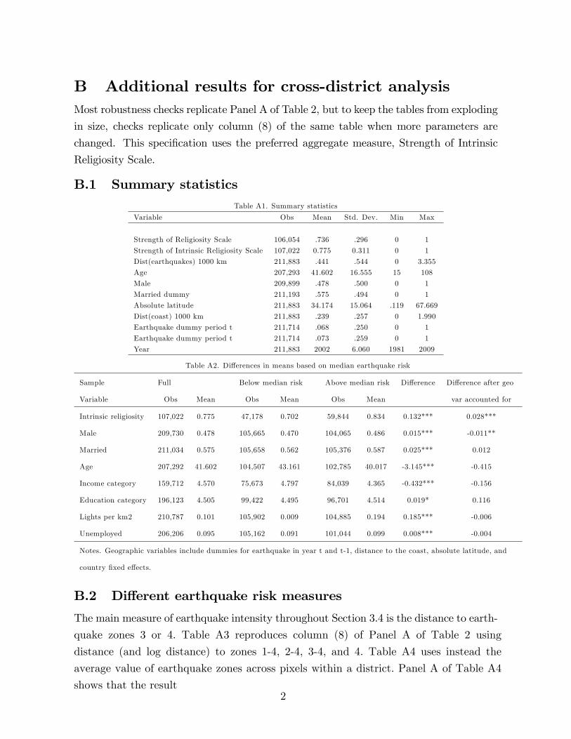
B Additional results for cross-district analysisMost robustness checks replicate Panel A of Table 2, but to keep the tables from exploding

in size, checks replicate only column (8) of the same table when more parameters are

changed. This specification uses the preferred aggregate measure, Strength of Intrinsic

Religiosity Scale.

B.1 Summary statisticsTable A1. Summary statistics

Variable Obs Mean Std. Dev. Min Max

Strength of Religiosity Scale 106,054 .736 .296 0 1

Strength of Intrinsic Religiosity Scale 107,022 0.775 0.311 0 1

Dist(earthquakes) 1000 km 211,883 .441 .544 0 3.355

Age 207,293 41.602 16.555 15 108

Male 209,899 .478 .500 0 1

Married dummy 211,193 .575 .494 0 1

Absolute latitude 211,883 34.174 15.064 .119 67.669

Dist(coast) 1000 km 211,883 .239 .257 0 1.990

Earthquake dummy period t 211,714 .068 .250 0 1

Earthquake dummy period t 211,714 .073 .259 0 1

Year 211,883 2002 6.060 1981 2009

Table A2. Differences in means based on median earthquake risk

Sample Full Below median risk Above median risk Difference Difference after geo

Variable Obs Mean Obs Mean Obs Mean var accounted for

Intrinsic religiosity 107,022 0.775 47,178 0.702 59,844 0.834 0.132*** 0.028***

Male 209,730 0.478 105,665 0.470 104,065 0.486 0.015*** -0.011**

Married 211,034 0.575 105,658 0.562 105,376 0.587 0.025*** 0.012

Age 207,292 41.602 104,507 43.161 102,785 40.017 -3.145*** -0.415

Income category 159,712 4.570 75,673 4.797 84,039 4.365 -0.432*** -0.156

Education category 196,123 4.505 99,422 4.495 96,701 4.514 0.019* 0.116

Lights per km2 210,787 0.101 105,902 0.009 104,885 0.194 0.185*** -0.006

Unemployed 206,206 0.095 105,162 0.091 101,044 0.099 0.008*** -0.004

Notes. Geographic variables include dummies for earthquake in year t and t-1, distance to the coast, absolute latitude, and

country fixed effects.

B.2 Different earthquake risk measures

The main measure of earthquake intensity throughout Section 3.4 is the distance to earth-

quake zones 3 or 4. Table A3 reproduces column (8) of Panel A of Table 2 using

distance (and log distance) to zones 1-4, 2-4, 3-4, and 4. Table A4 uses instead the

average value of earthquake zones across pixels within a district. Panel A of Table A4

shows that the result2

that the result is maintained across all religiosity measures when all controls, except

country-by-year fixed effects, are included. Panel B shows that the mean-measure does

not hold enough within-country variation to exert an effect on churchgoing and the

feeling that God gives comfort within countries. The no-effect on churchgoing is

consistent with the religious coping literature. Panel C shows that the distance to

earthquake zones wins the horse race between the two measures. This may be because

the mean-based measure does not vary for the districts that lie outside the earthquake

zones 1-4. For these districts, the measure takes the value zero. However, the actual

probability of an earthquake hitting is not equal to zero. This can be realized when

comparing Figures 3 and 6; some earthquakes hit in earthquake zones zero. The

distance-based measure captures better this variation.

3

Table A3. Main results with alternative earthquake measures

(1) (2) (3) (4) (5) (6) (7) (8) (9) (10)

Dependent variable: Strength of Intrinsic Religiosity Scale

Distance to earthq zones 1-4 -0.061**

(0.029)

Distance to earthq zones 2-4 -0.084***

(0.029)

Distance to earthq zones 3-4 -0.063***

(0.016)

Distance to earthq zone 4 -0.027***

(0.008)

Log (1+) Dist(earthq zones 1-4) -0.086**

(0.040)

Log (1+) Dist(earthq zones 2-4) -0.122***

(0.042)

Log (1+) Dist(earthq zones 3-4) -0.096***

(0.024)

Log (1+) Dist(earthq zone 4) -0.076***

(0.018)

Distance to fault line -0.037***

(0.011)

Log (1+) Dist(fault line) -0.058***

(0.019)

Observations 104,040 104,040 104,040 104,040 104,040 104,040 104,040 104,040 102,112 102,112

R-squared 0.325 0.325 0.325 0.325 0.325 0.326 0.325 0.326 0.318 0.318

Baseline controls Y Y Y Y Y Y Y Y Y Y

Regions 591 591 591 591 591 591 591 591 579 579

Countries 66 66 66 66 66 66 66 66 66 66

Notes. The dependent variable is the Strength of Intrinsic Religiosity Scale [0,1]. Baseline controls are the same as Panel A, Table 2.

4

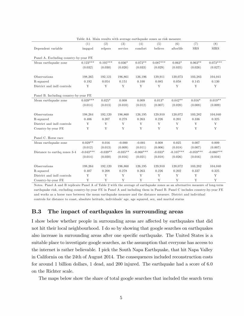
Table A4. Main results with average earthquake zones as risk measure

(1) (2) (3) (4) (5) (6) (7) (8)

Dependent variable impgod relpers service comfort believe afterlife SRS SIRS

Panel A. Excluding country-by-year FE

Mean earthquake zone 0.123*** 0.105*** 0.036* 0.072** 0.087*** 0.063* 0.063** 0.073***

(0.032) (0.030) (0.020) (0.033) (0.029) (0.035) (0.026) (0.027)

Observations 198,265 192,121 196,861 126,196 129,911 120,073 103,283 104,041

R-squared 0.192 0.054 0.151 0.100 0.085 0.058 0.145 0.130

District and indl controls Y Y Y Y Y Y Y Y

Panel B. Including country-by-year FE

Mean earthquake zone 0.039*** 0.025* 0.008 0.009 0.013* 0.042** 0.016* 0.019**

(0.014) (0.013) (0.010) (0.012) (0.007) (0.020) (0.008) (0.009)

Observations 198,264 192,120 196,860 126,195 129,910 120,072 103,282 104,040

R-squared 0.406 0.207 0.278 0.263 0.226 0.201 0.336 0.325

District and indl controls Y Y Y Y Y Y Y Y

Country-by-year FE Y Y Y Y Y Y Y Y

Panel C. Horse race

Mean earthquake zone 0.029** 0.016 -0.000 -0.001 0.008 0.025 0.007 0.009

(0.012) (0.013) (0.009) (0.011) (0.006) (0.018) (0.007) (0.007)

Distance to earthq zones 3-4 -0.043*** -0.039** -0.035** -0.060*** -0.033* -0.107*** -0.059*** -0.060***

(0.014) (0.020) (0.016) (0.021) (0.018) (0.026) (0.016) (0.016)

Observations 198,264 192,120 196,860 126,195 129,910 120,072 103,282 104,040

R-squared 0.407 0.208 0.278 0.263 0.226 0.202 0.337 0.325

District and indl controls Y Y Y Y Y Y Y Y

Country-by-year FE Y Y Y Y Y Y Y Y

Notes. Panel A and B replicate Panel A of Table 2 with the average of earthquake zones as an alternative measure of long-term

earthquake risk, excluding country-by-year FE in Panel A and including them in Panel B. Panel C includes country-by-year FE

and works as a horse race between the mean earthquake measure and the distance measure. District and individual

controls for distance to coast, absolute latitude, individuals’age, age squared, sex, and marital status

B.3 The impact of earthquakes in surrounding areas

I show below whether people in surrounding areas are affected by earthquakes that did

not hit their local neighbourhood. I do so by showing that google searches on earthquakes

also increase in surrounding areas after one specific earthquake. The United States is a

suitable place to investigate google searches, as the assumption that everyone has access to

the internet is rather believable. I pick the South Napa Earthquake, that hit Napa Valley

in California on the 24th of August 2014. The consequences included reconstruction costs

for around 1 billion dollars, 1 dead, and 200 injured. The earthquake had a score of 6.0

on the Richter scale.

The maps below show the share of total google searches that included the search term

5

"South Napa earthquake" in year 2014.55 Results are similar for searches on "earthquake".

The state with the highest share of searches on "South Napa earthquake" is California,

followed by Hawaii and states located close to California. These other states were not

hit by the earthquake, but searched for information about it nevertheless. Similarly with

metropolitan areas; areas closer to the epicenter searched more for information.

Figure A1. Google searches on "South Napa earthquake"

55Ideally, I would have liked to restrict the analysis to the period just after the earthquake, but Googletrends only allows restricting the searches to one specific year. The vast majority of searches on "SouthNapa earthquake" in 2014 occurred in the month after the South Napa earthquake.

6

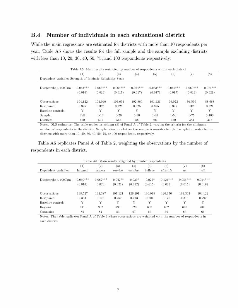
B.4 Number of individuals in each subnational district

While the main regressions are estimated for districts with more than 10 respondents per

year, Table A5 shows the results for the full sample and the sample excluding districts

with less than 10, 20, 30, 40, 50, 75, and 100 respondents respectively.

Table A5. Main results restricted by number of respondents within each district

(1) (2) (3) (4) (5) (6) (7) (8)

Dependent variable: Strength of Intrinsic Religiosity Scale

Dist(earthq), 1000km -0.063*** -0.063*** -0.064*** -0.064*** -0.063*** -0.065*** -0.069*** -0.071***

(0.016) (0.016) (0.017) (0.017) (0.017) (0.017) (0.019) (0.021)

Observations 104,122 104,040 103,651 102,860 101,421 99,022 94,590 88,688

R-squared 0.325 0.325 0.325 0.325 0.325 0.325 0.323 0.321

Baseline controls Y Y Y Y Y Y Y Y

Sample Full >10 >20 >30 >40 >50 >75 >100

Districts 600 591 565 529 501 450 383 315

Notes. OLS estimates. The table replicates column (8) of Panel A of Table 2, varying the criteria for the minimum

number of respondents in the district. Sample refers to whether the sample is unrestricted (full sample) or restricted to

districts with more than 10, 20, 30, 40, 50, 75, or 100 respondents, respectively.

Table A6 replicates Panel A of Table 2, weighting the observations by the number of

respondents in each district.

Table A6. Main results weighted by number respondents

(1) (2) (3) (4) (5) (6) (7) (8)

Dependent variable: impgod relpers service comfort believe afterlife rel reli

Dist(earthq), 1000km -0.050*** -0.062*** -0.047** -0.039* -0.026* -0.124*** -0.055*** -0.054***

(0.016) (0.020) (0.021) (0.022) (0.015) (0.023) (0.015) (0.016)

Observations 198,527 192,387 197,121 126,291 130,019 120,170 103,363 104,122

R-squared 0.393 0.173 0.267 0.233 0.204 0.176 0.313 0.297

Baseline controls Y Y Y Y Y Y Y Y

Regions 911 907 893 620 602 602 600 600

Countries 85 84 83 67 66 66 66 66

Notes. The table replicates Panel A of Table 2 where observations are weighted with the number of respondents in

each district.

7

B.5 Standardized coeffi cientsTable A7. Main results with standardized betas

(1) (2) (3) (4) (5) (6) (7) (8)

Dep. var. impgod relpers service comfort believe afterlife rel reli

Dist(earthq) -0.082*** -0.053** -0.053** -0.073*** -0.057** -0.131*** -0.113*** -0.110***

(0.022) (0.023) (0.023) (0.025) (0.028) (0.029) (0.029) (0.029)

Age -0.143*** -0.054*** -0.051*** -0.104*** -0.150*** -0.138*** -0.146*** -0.151***

(0.016) (0.017) (0.019) (0.020) (0.020) (0.023) (0.022) (0.022)

Age squared 0.240*** 0.163*** 0.149*** 0.222*** 0.222*** 0.142*** 0.256*** 0.253***

(0.018) (0.016) (0.019) (0.020) (0.023) (0.023) (0.023) (0.023)

Male dummy -0.107*** -0.110*** -0.056*** -0.121*** -0.100*** -0.096*** -0.131*** -0.136***

(0.004) (0.004) (0.008) (0.006) (0.006) (0.006) (0.007) (0.006)

Married dummy 0.033*** 0.048*** 0.057*** 0.049*** 0.036*** 0.013*** 0.055*** 0.050***

(0.004) (0.004) (0.004) (0.004) (0.005) (0.005) (0.005) (0.005)

Absolute latitude -0.092** -0.051* -0.041 -0.076*** -0.112*** 0.094** -0.066* -0.069*

(0.036) (0.030) (0.031) (0.027) (0.030) (0.039) (0.037) (0.036)

Distance to the coast 0.040*** 0.055*** 0.041*** 0.032*** 0.049*** 0.083*** 0.063*** 0.064***

(0.013) (0.013) (0.012) (0.012) (0.015) (0.016) (0.015) (0.015)

Earthq t -0.009* -0.001 0.010* -0.008 -0.011** -0.003 -0.005 -0.009

(0.006) (0.006) (0.006) (0.006) (0.005) (0.006) (0.007) (0.006)

Earthq t-1 -0.007 0.002 -0.008 -0.008 -0.014** 0.004 -0.007 -0.006

(0.004) (0.007) (0.005) (0.006) (0.005) (0.005) (0.006) (0.006)

Observations 198,264 192,120 196,860 126,195 129,910 120,072 103,282 104,040

R-squared 0.407 0.208 0.278 0.263 0.226 0.202 0.337 0.325

Country and year fixed effects Y Y Y Y Y Y Y Y

Dist=-.081 p-value 1 0.211 0.225 0.737 0.379 0.0940 0.273 0.319

Notes. The table replicates Panel A of Table 2 with standardized betas.

8

B.6 Binned scatterplots

Figure A2. Binned scatterplots for remaining religiosity measures

B.7 Actual earthquakes

While the main results include controls for actual earthquakes in year t and t-1, Table

A8 replicates the result of column (8) of Panel A of Table 2 controlling for additional

past earthquakes. Compared to Table 2, the sample is restricted to the sample without

districts hit by an earthquake in the year of interview. The pooled WVS-EVS only

9

provides data on the year in which the interview took place. Thus, it is not possible to

tell whether an earthquake that hit in the same year, hit before or after the interview,

which jeopardizes the intrepretation. Column (12) interacts long-term earthquake risk

with a dummy indicating whether an earthquake hit in the year before the interview.

The interaction is positive, but insignificant. However, only 24 districts in the sample

were hit within the last year, so this result should be taken with caution.

10

Table A8. Main results accounting for actual earthquakes

(1) (2) (3) (4) (5) (6) (7) (8) (9) (10) (11) (12)

Dep. var.: Strength of Intrinsic Religiosity Scale

Dist(earthq), 1000km -0.062*** -0.063*** -0.062*** -0.062*** -0.063*** -0.063*** -0.063*** -0.065*** -0.064*** -0.065*** -0.065*** -0.063***

(0.017) (0.017) (0.017) (0.017) (0.017) (0.017) (0.017) (0.018) (0.018) (0.018) (0.018) (0.017)

Earthquake year t-1 -0.003 -0.006 -0.005 -0.004 -0.004 -0.002 -0.002 -0.004 -0.003 -0.006 -0.005

(0.008) (0.008) (0.008) (0.008) (0.008) (0.007) (0.007) (0.007) (0.007) (0.008) (0.009)

Earthquake year t-2 0.007 0.009 0.009 0.009 0.009 0.011 0.011 0.011 0.014

(0.009) (0.009) (0.009) (0.010) (0.010) (0.010) (0.009) (0.009) (0.009)

Earthquake year t-3 -0.006 -0.006 -0.006 -0.006 -0.006 -0.006 -0.006 -0.009

(0.010) (0.010) (0.010) (0.010) (0.010) (0.010) (0.010) (0.011)

Earthquake year t-4 -0.005 -0.005 -0.004 -0.003 -0.009 -0.013 -0.011

(0.008) (0.008) (0.008) (0.008) (0.008) (0.008) (0.009)

Earthquake year t-5 -0.000 0.000 -0.000 -0.001 -0.003 -0.004

(0.013) (0.013) (0.013) (0.012) (0.012) (0.012)

Earthquake year t-6 -0.005 -0.004 -0.010 -0.010 -0.011

(0.009) (0.009) (0.009) (0.009) (0.009)

Earthquake year t-7 -0.011 -0.010 -0.011 -0.010

(0.018) (0.018) (0.018) (0.017)

Earthquake year t-8 0.019* 0.016 0.016

(0.011) (0.011) (0.011)

Earthquake year t-9 0.013 0.014

(0.010) (0.011)

Earthquake year t-10 -0.011

(0.009)

Dist(earthq) X earthq t-1 0.080

(0.098)

Observations 96,811 96,811 96,811 96,811 96,811 96,811 96,811 96,811 96,811 96,809 96,809 96,811

R-squared 0.321 0.321 0.321 0.321 0.321 0.321 0.321 0.321 0.321 0.321 0.321 0.321

Baseline controls Y Y Y Y Y Y Y Y Y Y Y Y

Notes. The table replicates column (8) of Panel A, Table 2 on a sample restricted to districts that were not hit in the year of interview.

11

Table A9 shows the correlations between actual earthquakes and the two earthquake

risk measures.

Table A9. Correlation matrix between earthquake measures

Dist Mean Sum

Distance to earthquake zones 3 and 4 1.00

Mean of all earthquake zones -0.63*** 1.00

Sum of all earthquakes 1973-2014 -0.15*** 0.49*** 1.00

B.8 Controls

B.8.1 Main results without baseline controls

Table A10 replicates Panel A of Table 2 without controls in Panel A and with country-by-

year fixed effects in Panel B. Churchgoing turns insignificant in the specification without

country-by-year fixed effects. This could be either due to problems of comparability across

countries or it could be in consistence with the findings in the religious coping literature

that churchgoing is less affected than intrinsic religiosity.

Table A10. Main results adding controls consequtively

(1) (2) (3) (4) (5) (6) (7) (8)

Dependent variable: impgod relpers service comfort believe afterlife rel reli

Panel A. No controls

Dist(earthq), 1000km -0.069*** -0.028* -0.024 -0.123*** -0.086*** -0.077*** -0.094*** -0.099***

(0.020) (0.017) (0.020) (0.028) (0.021) (0.026) (0.023) (0.022)

R-squared 0.012 0.001 0.001 0.016 0.015 0.006 0.021 0.021

Panel B. Country-by-year fixed effects

Dist(earthq), 1000km -0.056*** -0.049** -0.039** -0.070*** -0.042** -0.122*** -0.068*** -0.072***

(0.015) (0.020) (0.015) (0.021) (0.018) (0.032) (0.017) (0.018)

R-squared 0.383 0.182 0.263 0.230 0.207 0.185 0.304 0.292

Observations 203,100 196,721 201,254 130,139 133,948 123,744 105,947 107,022

Regions 884 880 868 611 592 592 591 591

Countries 85 84 83 67 66 66 66 66

Notes. Panel A of Table 2 without controls in Panel A and with country-by-year fixed effects in Panel B.

12

B.8.2 Additional controls

Panel A of Table A11 replicates Panel A of Table 2 on the restricted sample, where

information on individual income is available. Panel B adds the ten income dummies

(variable x047 in the WVS-EVS dataset).

Table A11. Main results including income dummies

(1) (2) (3) (4) (5) (6) (7) (8)

Dependent variable: impgod relpers service comfort believe afterlife rel reli

Panel A. Restricted sample with information on income

Dist(earthq), 1000km -0.046*** -0.037* -0.029* -0.039** -0.020 -0.102*** -0.055*** -0.054***

(0.014) (0.019) (0.015) (0.020) (0.016) (0.029) (0.014) (0.015)

R-squared 0.415 0.212 0.275 0.255 0.223 0.220 0.312 0.308

Panel B. Including income dummies

Dist(earthq), 1000km -0.044*** -0.036* -0.028* -0.035* -0.018 -0.100*** -0.052*** -0.051***

(0.014) (0.019) (0.015) (0.020) (0.016) (0.029) (0.014) (0.015)

R-squared 0.417 0.212 0.275 0.257 0.224 0.220 0.314 0.310

Observations 150,035 145,632 148,251 85,447 88,709 82,755 70,827 71,376

Baseline controls Y Y Y Y Y Y Y Y

Notes. Panel A replicates Panel A of Table 2, but on the restricted sample, where information on individual income

is available. Panel B adds the ten income dummies (variable x047 in the WVS-EVS dataset).

Table A12 replicates column (8) of Panel A of Table 2 adding individual-level controls

for trust (variable a165 from the pooled EVS-WVS), an unemployment dummy,56 and

ethnicity fixed effects (variable x051). The coeffi cient on long term eartquake risk stays

remarkably stable throughout.

Table A13 adds the following district-level controls to the same specification: popu-

lation density in year 2000, arable land shares (calculated based on irrigated and rainfed

agriculture, plate 47 from the FAO GAEZ 2002 database), average temperatures 1961-

1990 (spatial data from GAEZ), average precipitation and variation therein (spatial data

from GAEZ), district area in square km, average district-level ruggedness (based on Nunn

& Puga (2012)), average elevation, soil quality (plate 27 from the FAO GAEZ 2002 data-

base), and a dummy equal to zero if the distance to earthquake zones 3 or 4 is equal to

zero.57 Column (11) includes all significant variables simultaneously with no change to

56The unemployment dummy is equal to one if the person indicated his/her unemployment status as"Unemployed", zero otherwise (variable x028 in the pooled WVS-EVS).57In line with the work by Ager & Ciccone (forthcoming), the results show that increased within-year

variation in precipitation increases religiosity.

13

the results. The estimate on earthquake risk stays remarkably constant throughout. The

largest reduction in the estimate on earthquake risk is caused by including ruggedness,

which reduce β̂ from 0.063 to 0.055. Were any omitted variable to explain β̂ entirely, its

inclusion should result in an eight times larger reduction in β̂ compared to the reduction

caused by ruggedness (Altonji et al. (2005)).

Table A12. Main results including additional individual level controls

(1) (2) (3) (4) (5)

Dependent variable: Strength of Intrinsic Religiosity

Dist(earthq), 1000km -0.063*** -0.064*** -0.063*** -0.053*** -0.057***

(0.016) (0.016) (0.016) (0.014) (0.018)

Trust 0.001

(0.003)

Unemployed dummy 0.002

(0.004)

Agricultural worker 0.025***

(0.004)

Observations 104,040 100,371 101,045 76,464 61,340

R-squared 0.325 0.325 0.330 0.311 0.330

Baseline controls Y Y Y Y Y

116 ethnicity FE N N N N Y

Regions 591 591 586 475 375

Notes. The table replicates column (8) of Panel A of Table 2 including additional control variables.

14

Table A13. Main results including additional geographic controls

(1) (2) (3) (4) (5) (6) (7) (8) (9) (10) (11)

Dependent variable: Strength of Intrinsic Religiosity

Dist(earthq), 1000km -0.063*** -0.063*** -0.063*** -0.063*** -0.061*** -0.060*** -0.055*** -0.064*** -0.060*** -0.067*** -0.054***

(0.016) (0.016) (0.016) (0.016) (0.016) (0.016) (0.017) (0.016) (0.016) (0.017) (0.017)

Popdens 2000 -0.003** -0.002*

(0.001) (0.001)

Arable land (%) -0.003

(0.010)

Avg temp 1961-90 0.001

(0.001)

Prec 1961-90 0.016

(0.010)

Var(prec) 1961-90 0.134*** 0.105**

(0.048) (0.046)

Area 1000km -0.000

(0.000)

Average ruggedness 0.091*** 0.073**

(0.027) (0.029)

Average elevation 0.014* 0.001

(0.008) (0.008)

Soil quality 0.023

(0.018)

Disaster>0 0.012

(0.010)

Observations 103,489 104,040 103,365 103,365 102,434 104,040 101,484 101,907 103,284 104,040 100,768

R-squared 0.325 0.325 0.325 0.325 0.326 0.326 0.319 0.318 0.325 0.325 0.319

Baseline controls Y Y Y Y Y Y Y Y Y Y Y

Regions 590 591 589 589 583 591 574 577 588 591 572

Ethnicity FE N

Notes. The table replicates column (8) of Panel A of Table 2 including additional control variables.

Table A14 replicates column (8) of Panel A of Table 2 including all eleven answers from one particular question in the

pooled WVS-EVS. The question sounds: Here is a list of qualities that a child can be encouraged to learn at home. Which, if

15

any, do you consider to be especially important? Please choose up to five.58 The list of qualities includes: Manners (column

1), independence (column 2), hard work (3), feeling of responsibility (4), imagination (5), tolerance and respect for other

people (6), thrift saving money and things (7), determination and perseverance (8), religious faith (9 ), unselfishness (10), and

obedience (11).

Table A14. Adding alternative values as controls and dependent variables

(1) (2) (3) (4) (5) (6) (7) (8) (9) (10) (11)

Alternative value: Manners Independence Work Responsibility Imagination Respect Thrift Perseverence Faith Unselfish Obedience

Dependent variable: Strength of Intrinsic Religiosity Scale

Dist(earthq), 1000km -0.073*** -0.072*** -0.074*** -0.075*** -0.072*** -0.074*** -0.074*** -0.074*** -0.064*** -0.074*** -0.073***

(0.019) (0.019) (0.019) (0.019) (0.019) (0.019) (0.019) (0.019) (0.020) (0.019) (0.019)

Alternative value 0.030*** -0.052*** -0.004 -0.019*** -0.047*** 0.002 -0.011*** -0.041*** 0.181*** -0.008** 0.024***

(0.004) (0.004) (0.003) (0.003) (0.005) (0.003) (0.004) (0.003) (0.009) (0.004) (0.003)

R-squared 0.312 0.317 0.311 0.312 0.314 0.311 0.311 0.314 0.364 0.311 0.312

Observations 69,857 69,857 69,857 69,857 69,857 69,857 69,857 69,857 69,857 69,857 69,857

Notes. OLS estimates. The table replicates column (8) of Panel A of Table 2.

58Respondents that answered yes to more than five of the values were removed.

16

B.9 Aggregation at the district and country level

The district-level aggregation is done in the following way: religiositydct = 1N

N∑i=1

widct ·̂religiosityidct, where the weights, widct, are based on variable s017 used throughout.̂religiosityidct measures the residuals of a regression of religiosityidct on the particular

individual-level controls for age, age squared, married, and male. Panel A of Table 2 has

591 districts and 75 countries. In addtion to the controls included in Panel A of Table 2,

the country-level aggregates also include a dummy for whether the country is communist

together with continent fixed effects. Excluding these additional control variables leaves

the parameter estimate on earthquake risk and the level of significance unchanged (-0.032

(se 0.017)).

17

Panel A. Full sample

RU

VN

ZAZA

AU

US

CA

VN

FR

AR

ES

ESESES

AR

UA

UA

NG

USAURU

RU

ININFR

DE

IN

DE

US

IN

VN

DZ

DZRUUS

IN

DZARIN

IN

ARES

ES

ES

ES

US

FI

ES

ES

ES

ES

INDZ

IN

DE

DZ

UA

UA

ZW

DE

INSA

IN

IN

DZ

IN

AUUA

UA

UAUAFR

CA

US

US

CA

IN

IN

IN

AUSA

FR

IN

ZAZA

ES

ESES

ES

PLDZZW

IN

PL

AT

AR

UY

FRUY

CA

AR

ZAZAEGNG

US

CA

IQ

PL

IQNG

UAUA

CZ

UA

UA

IQ

BYINCOIQ

MX

DE

MX

FI

PLBY

FR

LV

UA

UAPL

ES

ES

ES

ES

DESK

LV

UA

UA

DE

CZ

UG

IQ

IN

LV

NGIQ

SA

IQ

MX

NL

DE

EE

LT

ES

ES

ES

ESIQUSUS

ZWIQ

COIN

UAUA

PT

PT

BD

BD

IQ

IN

IT

IQ

ITSA

AT

ES

ESES

ES

EE

UA

UASK

CH

DE

GB

ITBD

BD

CH

UA

UA

IT

LV

DE

IE

DK

PEPE

EE

FR

GT

PE

FR

HU

DE

DE

AZ

LV

CZ

PE

HR

DE

JOPHJO

MDJO

AT

PT

JOJO

MD

INJP

IQCH

LV

DE

LV

JPUSLVARDK

IQ

FRBEPKNG

LT

SK

PHJO

CH

BG

IN

BG

JPIT

JP

CA

PL

LV

JP

CH

KG

CZ

NLCLSVSV

SV

SVRS

KG

GR

IT

GR

AT

ID

NGNLGRIQ

LV

PH

BD

BD

MXJP

KG

HU

GE

SVCL

NZ

IR

AZ

ES

ES

ES

ES

CLEEEEMX

PKJO

IQJP

HU

IQ

KG

IR

INZW

IT

IT

KG

UGCL

IR

SV

IR

IQ

UAUABA

IT

DK

CH

IRNL

IRGEGR

BG

IR

IR

IR

IR

IR

IR

IR

IR

IN

CH

RS

DOIRIR

CZ

IR

IT

PH

IRIR

PK

IT

RU

EEIR

IR

IR

IR

GT

RU

IRIRIR

CZ

CH

IR

KG

IRMX

BA

BAIR

IRLVIRIR

LVIR

FIZA

ZAIR

GR

DE

LV

IR

IQBG

PL

PE

BDBDGR

UA

UANG

IR

NG

IN

GR

SK

SV

UA

UA

AM

IR

DO

MKMK

IDLVUY

AM

MK

MK

ITPEIQ

AM

LV

AM

CA

MK

MK

AMIT

AM

PE

MK

MKAM

AMAT

AM

NZ

IT

AL

AL

AL

AL

AL

CZ

AL

AL

AZ

JPNGARGBUSMAMDDO

AZ

GBCHHU

AL

NL

DE

BA

NZID

NL

AL

AL

JONG

SV

IR

IT

GE

JP

UY

CZ

EE

RU

UY

HRJP

RU

LV

UA

UAEGIRIQ

JPGR

GR

GR

BG

SV

SV

CH

PEBESVEEIQ

UY

BA

BA

FRCL

CL

BY

BG

CL

NL

IQ

NG

GR

PHAM

ZW

LV

IDJP

CL

CL

MK

MK

FRLVID

IN

CL

IQ

AMLV

CL

FR

BA

LT

NL

GE

JP

DOPL

NL

CZ

LVAZ

BYITSV

NL

SK

GE

IR

BY

LV

DK

BG

NZ

EE

IRIR

IRIR

UG

LV

IRZAZAIQBEIR

NGLV

DE

PH

IREE

PHGTIRFI

NGIR

DE

IR

KG

MD

IR

IQ

CZ

GT

CH

LVEE

GR

RU

HUIQ

IR

CH

CZ

NL

DE

AR

EE

ES

ES

ES

ES

NL

UA

UA

PEIT

LT

HR

DE

JO

PE

RS

LVSK

CZ

IN

DE

GR

BGCO

EE

SK

PT

PL

PH

CHJOZW

JP

AZLV

AT

LT

ZW

DE

IE

MDSVSVGB

PLEE

FR

JPATIQ

UA

UAHUFIPL

FR

LVCH

IQAT

JO

JP

IRIR

LV

CA

FR

CZ

LV

UAUA

ZWBD

BD

CH

PK

SK

UG

UA

UA

SA

CZ

BD

BD

DK

UA

UA

LV

MX

IQ

AT

DE

AR

UY

PLIQ

SA

ES

ES

ES

ES

US

AR

DE

ESES

ES

ES

KG

IN

IT

ZWZW

ZAZA

EG

MX

VN

ES

ES

ESES

UA

UA

FR

ZA

ZA

MXNGCO

PEJO

SA

IQ

NG

US

DE

IQ

DE

PT

DE

BY

FR

IN

DE

DE

UYFR

PLSA

IN

PL

NGININAU

UA

UA

ES

ES

ES

ESIN

FR

FR

ES

ES

ES

ES

DE

NGDE

ES

ESES

ESIN

IQ

IQ

ES

ES

ES

ESUA

UA

IN

DZ

FI

US

VN

CAZA

ZA

IN

IT

UA

UAZAZADZ

INRU

AR

USAR

AU

RU

RU

INFRUS

INUS

AR

US

INAR

UA

UA

USIN

VN

VN

IN IN

AU

CARU

DZ

­.4­.2

0.2

.4St

reng

th o

f Int

rinsi

c R

elig

iosi

ty S

cale

 | Xi

­.8 ­.6 ­.4 ­.2 0 .2 .4 .6 .8 1Dist(earthquakes) | Xr

coef = ­.06036494, (robust) se = .01908479, t = ­3.16

IS

IS

IS

USZAAT

GEZACL

KG

MDIT

PT

IR

ZW

IT

US

JP

CL

SI

TR

GE

AT

AM

ES

IT

ZA

SI

ROMD

UA

CL

BG

IT

AT

UG

AR

TZCH

SI

RO

PT

AR

HR

BY

JP

CZ

BG

BG

HU

HR

USMK

AM

DE

AL

BA

MK

AR

BA

JP

CY

ES

IS

EG

DE

US

UA

ES

TR

CZ

HR

HU

GR

MT

MDSK

BG

UA

RO

CZ

BY

AZ

HU

PL

GR

JP

CH

TR

MT

MK

PT

AL

BA

BD

DO

SKES

AL

BY

BE

JO

CA

RU

BE

MT

DE

PE

AUES

SKBE

DZ

FR

NL

CZ

ROMTIQSIVN

FR

CA

HU

DE

PE

ES

NL

LU

NZ

VE

PK

PL

RU

LU

DK

MXBY

SK

UY

DE

PL

RU

DK

BE

FR

NL

RU

LV

AR

MX

LT

NL

BD

CANO

CO

LT

DKMX

PH

SV

LV

EE

FR

DK

GB

IN

LV

MX

GB

SE

LT

IE

GB

IE

NO

EE

PH

SA

EE

NO

FI

SE

GB

SE

IE

IN

IE

SE

FI

FI

FI

IN

SE

NO

ID

NG

BR

NG

­.3­.2

­.10

.1.2

Stre

ngth

 of I

ntrin

sic 

Rel

igio

sity

 Sca

le | 

Xi

­1 ­.6 ­.2 .2 .6 1 1.4 1.8Dist(earthquakes) | Xr

coef = ­.03704024, (robust) se = .01721637, t = ­2.15

Panel B. Excluding outliers (diff<=1)

RU

AU

ZA

ZA

US

VN

CA

FR

AR

ES

ESES

ES

ARUA

UA

AU

NG

RU

US

ININ

FR

INVN

IN

RU

US

AR

DZ

DZ

IN

DZAR

IN

ESES

ES

ES

IN

ES

ES

ES

ES

INDZ

US

IN

UA

UA

DZ

US

INZW

SA

IN

IN

DZ

AU

UA

UA

FR

CA

IN

UAUA

IN

IN

CA

US

FR

DE

PL

ES

ES

ES

ES

IN

ZAZA

SA

IN

DZ

PL

ZW

AR

AT

AU

UY

CA

FR

ZAZA

UY

DE

AR

EGNG

CA

PL

DE

IQ

NGIQ

US

UAUADE

BYINCO

UA

UA

IQ

IQ

CZ

DE

PL

US

BY

FR

LVUA

UA

PL

DE

ES

ES

ES

ES

LV

UA

UA

CZ

UG

IN

LV

NGSAIQ

NL

EE

IQ

IQ

MXLT

ES

ES

ES

ES

IT

IQPT

IN

CO

ZWIT

IQ

UAUAPT

BD

BDIQ

IT

SA

IQ

AT

UA

UA

EE

DE

ES

ES

ES

ES

SK

DK

UA

UA

US

PE

IT

BD

BD

PELV

GB

CH

IE

FR

EE

CH

MX

PE

IN

HU

FR

INLV

CZ

AZ

HR

PT

AT

JOJOJO

JO

DK

PE

JO

IQ

LV

FR

LV

LV

IQ

AR

BE

IT

LT

BG

SK

IT

NG

CH

JOMDSKPLJP

LV

MD

NL

CA

CH

IR

RS

NZ

AT

CZ

NLCH

LVIR

BD

BD

IN

HU

NGGE

IR

IQIR

EEJOIQEE

AZ

BG

HU

UAUA

ZWPH

ESES

ES

ES

IQ

IQ

IRIR

ID

IT

CLUGIR

BAGE

NLKG

IT

IN

GR

IR

GRIRGRIR

IRRS

FI

IR

IRCHIR

DO

RU

KG

IR

EE

JP

CZ

IRIRIR

IR

IR

IR

IRIR

IRIR

IN

IR

CH

IR

JP

IR

BG

ZA

ZA

LV

CZ

IRCLIRLV

JPPH

DE

SV

KG

IRIR

SVIR

IR

SV

GRSV

CL

KG

BDBD

NG

IQ

LV

CH

IR

PL

MKAM

IR

PK

DO

UA

UA

UA

UA

NG

LV

SVNZ

IR

MK

IQPE

AM

IT

AM

LV

AM

MK

AM

AM

UYAM

AM

AM

ATAL

CA

MKALAL

AZ

CZ

PE

IT

SV

GB

AL

FIGBMAMXUSPHGT

AL

DOMK

AZ

NGHU

NLCLJO

GE

KG

JP

ALID

GR

CZ

GRNZ

EE

UY

HR

LV

PK

BG

CH

IR

EGIQ

UA

UAGR

DE

JP

IN

JP

IQ

IR

BE

EE

NG

BY

UYFR

IQ

ZW

NL

CL

LV

AM

MK

PE

CH

IQ

FI

SVSK

FRLV

ID

IR

LV

AM

IT

PL

LT

NL

NL

BA

DO

AZ

FR

SKGE

BYDK

LV

IR

CL

SK

GEBG

IR

NL

SV

IRIR

BY

LV

IR

UG

EE

IR

IR

LV

NZ

IR

BEIQ

LV

EENG

ZA

ZAPHIRNG

IR

CZ

LV

IQ

EE

PE

HU

IR

IQIT

CZ

AR

CH

RU

DE

NL

PE

EE

IR

ES

ES

ES

ES

NL

HR

UA

UA

LTCH

JO

GRBG

IN

RS

LVJP

CO

KGEE

JO

PL

CZ

PT

ZW

AZ

AT

ZW

LV

MX

LT

IECH

DE

GB

EE

IQAT

PL

FR

UA

UA

HU

FRIQ

PL

US

LV

AT

JOMDFRIR

CA

IR

LVCZ

LV

UAUA

BD

BDZW

SK

MX

CH

UG

DE

UA

UA

SA

DE

DKDE

BD

BD

UA

UA

CZIQAR

LV

AT

IQ

UY

PL

DE

SAAR

VN

ES

ES

ES

ES

ES

ES

ES

ES

IT

ZAZA

ZW

IN

USZWEG

ZA

ZA

ES

ES

ESES

UA

UA

FR

NG

SA

JOPE

IQ

CO

IN

NG

IQ

PT

FR

DE

BY

UYFR

DE

SA

IN

PL

IN

ES

ES

ES

ES

PL

NGINUS

UA

UA

IN

AU

FR

FR

IN

ESES

ES

ES

NG

VN

IN

IQ

ES

ES

ES

ES

IQ

DZ

ES

ES

ES

ES

UA

UA

IN

US

IT

CAZA

ZA

UA

UA

IN

DZZAZARU

AR

US

RU

AR

AU

IN

US

FR

IN

US

IN

US

AR

AR

UA

UA

VN

IN

IN

IN

AU

CA

RU

DZ

­.3­.2

­.10

.1.2

Stre

ngth

 of I

ntrin

sic 

Rel

igio

sity

 Sca

le | 

Xi

­.8 ­.6 ­.4 ­.2 0 .2 .4 .6 .8 1Dist(earthquakes) | Xr

coef = ­.05814145, (robust) se = .01497775, t = ­3.88

IS

IS

IS

ZAUS

GE

ZA

AT

KG

MDIT

CL

IT

IR

PT

ZW

ES

GE

HR

SI

US

ZA

AM

JP

AT

SI

TR

TR

MD

BY

IT

UA

RO

IT

BG

US

AT

GR

SI

CH

CY

CL

PT

EG

RO

HR

BG

BA

DE

DE

MK

BA

AL

GRMK

US

CL

AR

TZUG

ES

ES

HR

AM

UA

CZ

RO

MD

BA

HU

ALMK

AR

BD

UA

TR

CZ

PL

BY

HU

JO

CH

MT

ES

AL

BE

RU

BE

DO

BY

DE

BE

SK

HU

BG

PT

CZ

MT

AR

NL

NL

DZ

ES

HU

FRFR

SIMTIQ

MX

CA

PK

DE

SK

CA

ES

LURU

SK

DK

PL

DK

SK

LU

PERU

BE

PE

PL

BY

NL

FR

LV

RU

DE

NO

NL

MX

LT

BD

PH

UY

DKMX

LT

VE

EE

IN

SV

LV

DK

MX

SE

GB

GB

LV

GB

IE

IE

CA

FR

NO

EE

PH

FI

NO

EE

SACO

GB

SE

IE

SE

IN

SE

NO

IE

FI

FI

IN

FI

SE

ID

NG

NG

­.3­.2

­.10

.1.2

Stre

ngth

 of I

ntrin

sic 

Rel

igio

sity

 Sca

le | 

Xi

­1 ­.6 ­.2 .2 .6 1 1.4 1.8Dist(earthquakes) | Xr

coef = ­.05649714, (robust) se = .01709951, t = ­3.3

Panel C. Excluding outliers (diff<=0.1)

RU

ZA

ZA

USFR

AU

AR

INES

UA

ES

ES

CA

US

ES

CA

FR

NG

IN

AR

IN

IN

AU

RU

AR

UA

UA

ZW

IN

UA

IN

IN

USSA

IN

INES

UA

US

IN

AR

FR

RU

ES

ZW

UA

US

ZADZ

FR

DZ

PLUS

ES

DZ

PL

EG

ZA

IQ

ZA

UABY

DE

NG

IQNG

UA

IN

IQ

IN

DZ

ZA

DZ

IQ

NGIN

UA

ES

IN

UA

IQ

SA

UA

UA

AT

DZ

LV

UY

US

US

PL

ES

PL

LV

ZW

ES

IQ

UA

IQ

ES

IQ

IQ

SA

EE

FR

ES

PE

BD

PE

ITIQ

PEIN

UA

IQ

IT

IQFR

HR

IT

JO

JOMXJOJO

LV

HU

JO

SK

DZ

IQ

UA

LV

UA

JO

CH

ARGB

UA

ES

NG

IQ

DK

IR

IR

EE

LV

HU

IR

EE

DE

IR

IR

IT

IR

LV

LV

GE

PH

IR

IQ

IR

CH

IR

NL

LV

IR

IR

CZ

ZW

JO

IR

EEIR

ES

BG

PLIR

IR

IR

IR

BDIR

GR

GENL

BD

IR

IR

IRGR

BGGR

CLDK

IQ

IR

IR

CH

IN

DO

IR

IR

ESIRID

UA

ZA

NLIR

PE

SV

NG

CL

CLSV

IQ

CH

SV

PE

BY

SV

GR

NGCL

LV

IT

PL

KG

ES

IR

NG

NG

AM

DOSV

IR

UA

LV

LV

LV

UA

AM

BY

IR

AM

AL

BD

JP

IR

EE

AL

LV

IQ

BEGBLTCZVNMAUSAZMXMDRSPTPHMKJPJPAL

AMDO

IR

SV

JP

NG

FRAL

EE

HU

GR

IR

FR

JOHR

IRGEKG

ZAGR

NL

IR

CH

BY

EG

IR

PE

AM

IR

IQ

ID

IR

IQ

GE

AT

ZA

IQ

SV

LV

LV

ES

CH

LV

DO

AT

IR

BD

LV

CZ

NL

NL

EE

IR

SV

PL

IRNG

LV

PH

GE

IR

IR

EE

IQ

IT

DEIR

IQ

LV

UA

LV

ZA

GBAR

IR

LVIR

IR

BG

IR

EE

UA

IQ

NG

FR

CL

SK

IR

IR

UA

FR

HR

JOLV

IQ

DK

ITAT

MX

PL

EE

GR

ES

PL

FR

JO

PE

ZW

IQ

LV

CHZW

UA

ESPL

JOUA

IQ

AR

LV

HU

IR

UA

USUY

BD

ZW

AU

IR

CA

IQ

UA

IQ

PL

SAFR

ES

IQ

SA

NG

EG

DE

IN

BY

IT

ZA

ZW

ZW

FR

NG

US

FR

PE

JO

IQ

ZA

SA

UA

ZA

ES

ES

IQ

PL

NGIN

FR

FR

ES

UA

UA

IN

IN

IN

UA

US

AR

NG

ES

ES

UA

ES

ESUA

AR

IQ

ES

ZA

ES

ZA

US

ZA

USES

ZA

AR

FRININ

IN

AR

UA

US

RU

UA

DZ

IN

IN

US

IN

DZ

CA

AU

RU

­.1­.0

50

.05

.1St

reng

th o

f Int

rinsi

c R

elig

iosi

ty S

cale

 | Xi

­.8 ­.6 ­.4 ­.2 0 .2 .4 .6 .8 1Dist(earthquakes) | Xr

coef = ­.06254055, (robust) se = .00991181, t = ­6.31

US

GE

US

HR

AT

BA

AM

MK

AL

IT

AL

MK

PTCL

SI

AT

RU

AR

MD

CYPT

CL

SI

AT

IT

CL

DE

JO

HR

CH

SI

PT

BA

ZA

RU

BG

RO

HR

AL

DE

UA

MK

ZA

ZA

ES

HU

ES

SK

BE

NL

UA

HU

NO

TZ

BY

FIMTSIIQAM

CH

MX

ZW

CA

ES

HU

BE

NL

PH

SK

EG

BD

BD

SK

DK

MXLU

PH

ES

BE

NL

MT

SK

LU

SV

DK

ES

NL

CA

BY

DZ

DK

LT

LV

IN

MX

PE

GB

LV

CA

NO

NO

NO

GB

GBIN

ID

FI

SE

CO

­.2­.1

0.1

.2St

reng

th o

f Int

rinsi

c R

elig

iosi

ty S

cale

 | Xi

­1 ­.8 ­.6 ­.4 ­.2 0 .2 .4 .6 .8 1Dist(earthquakes) | Xr

coef = ­.06791939, (robust) se = .01708193, t = ­3.98

District aggregates Country aggregates

Figure A3. Added variable plots of religiosity on long-term earthquake risk

Notes. AV-plots of OLS estimation across district aggregates in the left panels and across country aggregates in the right.

The estimation corresponds to that in column (8) of Panel A in Table 2, where the individual-level controls are accounted for

before aggregation. Panel A includes the full sample, Panel B excludes outliers based on Cooks D > 1, and Panel C

excludes outliers based on Cooks D > 0.1. Labels: Country ISO codes.

18

B.9.1 Further investigation of country weights

Table A15 shows results aggregated to the country-level, using country weights (variable

s017) in Panel A, and aggregating without country weights in Panel B.

Table A15. Main results aggregated to the country level

(1) (2) (3) (4) (5) (6) (7)

Dep.var. impgod rel_pers service comfort believe after reli

Panel A. Baseline

Dist(earthq) -0.053*** -0.048*** -0.003 -0.045*** -0.055*** 0.001 -0.037**

(0.012) (0.013) (0.012) (0.017) (0.015) (0.019) (0.018)

Observations 320 320 318 204 252 202 196

R-squared 0.643 0.425 0.611 0.539 0.493 0.414 0.462

Panel B. Baseline without weights

Dist(earthq) -0.054*** -0.049*** -0.003 -0.045*** -0.056*** 0.001 -0.037**

(0.012) (0.013) (0.012) (0.017) (0.015) (0.019) (0.018)

Observations 320 320 318 204 252 202 196

R-squared 0.643 0.424 0.610 0.539 0.492 0.413 0.462

Baseline controls Y Y Y Y Y Y Y

B.10 Actual losses from earthquakes

An alternative measure of the impact from an earthquake is the costs of the disaster. The

International Disaster Database EM-DAT provides information at the country-level of all

newer disasters of a certain impact and size. It also provides information on the costs of

the disasters, both human (number of injured, number of deaths) and economical. Data

was downloaded at www.emdat.be. The database is created from information from various

sources, ranging from UN agencies to press agencies. Most prioritized is the information

from UN agencies, governments and the International Federation of Red Cross.

I have divided the human and economic costs of the disasters with the population in

each country. Table A16 shows the correlation between a dummy equal to one if the coun-

try is located within a high-risk earthquake zone, zero otherwise, the distance-based and

the mean-based measures of earthquake risk and the three actual costs of earthquakes.

Countries located within high risk earthquake zones experience more human and eco-

nomic costs from earthquakes. Likewise for the mean-based measure. The distance-based

measure does not correlate significantly with any of the costs. This indicates that the

results using the distance-based measure are not likely to be driven by the actual costs of

earthquakes.

19

Table A16. Correlations between actual losses and different risk measures

Eq zone dummy Dist(earthq) Mean(earthq) Deaths Affected Damage

Earthquake zone dummy 1.00

Dist(earthquake zones) -0.54*** 1.00

Mean(earthquake zones) 0.72*** -0.48*** 1.00

Deaths per capita 0.13* -0.07 0.16** 1.00

Affected per capita 0.22*** -0.12 0.30*** 0.51*** 1.00

Damage per capita 0.15** -0.08 0.28*** 0.15** 0.32*** 1.00

Table A17 investigates the relationship between the intristic religiosity scale and the

human and economic cost of earthquakes from the EM-DAT database. There is a positive

relationship between religiosity and human costs from disasters, also when controlling for

GDP per capita (Panel A). The relation seems to be driven mainly by differences across

continents, though (Panel B). There seems to be no relation between the economic costs

from earthquakes and religiosity. If anything, economic damage reduces religiosity, but

this effect becomes insignificant once GDP per capita is included.

20

Table A17. OLS of religiosity on actual losses from earthquakes across countries

(1) (2) (3) (4) (5) (6)

Dependent variable: Strength of Intrinsic Religiosity Scale

Panel A. Including baseline individual level controls

Deaths per capita 0.785*** 0.562***

(0.212) (0.158)

Affected people per capita 0.006*** 0.004***

(0.002) (0.001)

Total damage per capita -0.000 -0.000

(0.000) (0.000)

GDP per capita PPP 2010 -0.006*** -0.005*** -0.006***

(0.001) (0.001) (0.001)

Observations 208 208 208 205 205 205

R-squared 0.011 0.039 0.006 0.191 0.202 0.186

Panel B. Including individual level controls and continent and year fixed effects

Deaths per capita 0.380 0.423

(0.476) (0.453)

Affected people per capita 0.004* 0.003*

(0.002) (0.002)

Total damage per capita -0.000* -0.000

(0.000) (0.000)

GDP per capita PPP 2010 -0.005*** -0.004*** -0.004***

(0.001) (0.001) (0.001)

Observations 203 203 203 200 200 200

R-squared 0.331 0.341 0.340 0.408 0.414 0.408

Notes. The individual level controls are the same as those included throughout. They are accounted for

before aggregating the data.

B.11 Different religiosity measures

The original variables used in Table 1 are: (1): f063, (2): f064, (3): f050, (4): f034, (5):

f051, and (6): f028. The original variable f034 (religious person) also had a category

for convinced atheists. Following Inglehart & Norris (2003), I group people who rank

themselves as not religious or atheist into one category, as there are very few respondents

in the latter group. The variables f063 (importance of god) and f028 (churchgoing) are

described and investigated further below.

B.11.1 Different categorizations of the religiosity measures

Two of the religiosity measures are not dummy measures: Attendance at religious service

and importance of God. This section shows that the results for importance of God are

robust to different categorizations, while attendance is not. The impact of earthquake

risk occurs at the intensive margin and not at the extensive margin for both measures.

Table A18 replicates column (3) of Panel A of Table 2 with different measures of

21

attendance at religious services. The different columns perform different aggregations of

the variable f028 from the WVS-EVS. The variable is based on the question: "How often

do you attend religious services?" The possible answers are "More than once a week" (1),

"Once a week" (2), "once a month" (3), "only on special holy days/Christmas/Easter"

(4), "other specific holy days" (5), "once a year" (6), "less often" (7), "never, practically

never" (8). The orginal variable takes on values from 1 to 8. All permutations of this

variable depicted in Table A18 are rescaled to lie between 0 and 1 and are flipped around so

larger values mean more churchgoing. Column (1) uses variable f28 directly. Column (2)

replicates column (3) of Panel A of Table 2, where categories (4) and (5) are aggregated,

due to few observations in the latter and since it is not obvious how to rank the two.

Columns (3) and (4) investigate the impact of earthquake risk on dummies indicating

frequent churchgoers, defined as attending religious services more than weekly (category

1) in column (3) and weekly (category 1 and 2) in column (4). Column (5) reduces the

measure to the extensive margin using a dummy measuring churchgoing or not. "Not" is

defined as "Never, practically never" (category 8). Column (6) investigates the intensive

margin, where those who never or practically never are removed from the sample.

Table A18. Main results with different categorizations of churchgoing

(1) (2) (3) (4) (5) (6)

Dep. var: Attendance at religious services

Dist(earthq), 1000km -0.037** -0.035** -0.044*** -0.024 -0.017 -0.043***

(0.016) (0.015) (0.017) (0.019) (0.016) (0.016)

Observations 196,860 196,860 196,860 196,860 196,860 152,476

R-squared 0.268 0.278 0.202 0.251 0.195 0.227

Baseline controls Y Y Y Y Y Y

Service measure org base frequent1 frequent2 extensive intensive

Standardized coef: Dist(earthq), 1000km -0.055** -0.053** -0.071*** -0.028 -0.022 -0.073***

(0.023) (0.023) (0.027) (0.022) (0.021) (0.027)

Notes. OLS estimates. The table replicates column (3) of Panel A of Table 2 with different measures

of attendance at religious services. The individual measures are described above the table

The measure of importance of God is based on the question "How important is God

in your life?", where individuals can answer a number between 1 and 10. 1 indicates "Not

at all important" and 10 indicates "Very important". I have rescaled the variable to lie

between 0 and 1. In table A19, column (1) replicates the baseline result in column (1)

of Panel A of Table 2. Columns (2) and (3) aggregate the variable to a dummy variable

measuring the difference between regarding God as important and the rest. "Important"

is defined as rating God as very important (category 10) in column (2) and categories 10

and 9 in column (3). Column (4) investigates the extensive margin by using a dummy

22

variable measuring whether the individual is religious or not. Non-religious is defined as

rating God as being not at all important (category 1). Column (5) restricts the sample

to the intensive margin, by excluding individuals who answer that God is not important

at all.

Table A19. Main results with different categorizations of importance of God

(1) (2) (3) (4) (5)

Dep. var: Importance of God

Dist(earthq), 1000km -0.052*** -0.074*** -0.074*** -0.025* -0.046***

(0.014) (0.020) (0.023) (0.013) (0.013)

Observations 198,264 198,264 198,264 198,264 180,273

R-squared 0.407 0.390 0.394 0.160 0.356

Baseline controls Y Y Y Y Y

Importance of God measure org frequent1 frequent2 extensive intensive

Standardized coef: Dist(earthq), 1000km -0.082*** -0.081*** -0.081*** -0.047* -0.084***

(0.022) (0.022) (0.025) (0.024) (0.023)

Notes. OLS estimates. The table replicates column (1) of Panel A of Table 2 with different measures

of importance of God. The individual measures are described above the table

B.11.2 Religiosity independent of churchgoing

This section exploits answers to the question "How often do you pray to God outside

religious services?"59 The respondents can answer "Every day", "more than once a week",

"once a week", "at least once a month", "several times a year", "less often", and "never".

I rescaled the variable to lie between 0 (never) and 1 (every day). One issue with the

measure is that people who go to church more often may be less likely to pray when they

are not in church. Since earthquake risk also influences churchgoing, this may affect the

results. Column (3) shows that earthquake risk increases the degree of prayer outside

religious services, but less so for those who go to church more often. These results are

consistent with religious coping and cannot be explained by alternative theories that

involve churchgoing. The variable measuring attendance at religious services takes the

values 0 to 1, where 1 indicates those who attend religious services more than once a

week. This variable is not available for enough observations to estimate the corresponding

regression in the event study.

59Thanks to an anonymous referee for suggesting to use this question.

23

Table A20. Main results with prayer outside religious services as alternative measure of religiosity

(1) (2) (3)

Dependent variable: Prayer outside religious services

Dist(earthquake zones), 1000km -0.103** -0.025 -0.101***

(0.044) (0.029) (0.030)

Dist(earthquake zones) x attendance at religious services 0.246***

(0.040)

Attendance at religious services 0.469***

(0.027)

Observations 66,192 66,192 64,058

R-squared 0.166 0.327 0.506

Baseline controls Y Y Y

Country-by-year FE N Y Y

B.12 Heterogeneity by religion and continents

To investigate whether people from different denominations engage differently in religious

coping, the following equation is estimated:

religiosityidct = α+β1disastersdc+β2disastersdc ·Igidct+β3I

gidct+γct+X

′dcη+W ′

idctδ+εidct

(1)

where Ig are dummy variables equal to one if individual i belonged to the religious

denomination g at time t. g refers to one of the major religions: Christianity (split

into Catholicism and Protestantism), Islam, Buddhism, Hinduism, Judaism, and Other

religions.60 β1 + β2 is the impact of earthquake frequency for individuals belonging to

religion g.

Table A21 shows estimation results for equation (1). Column (1) includes no inter-

action effects, but restricts the sample to the sample where information on individuals’

religious denomination is available. The estimate drops in absolute value from -0.063 (col-

umn 8, Panel A, Table 2) to -0.043 on this restricted sample. This is probably because

we are now comparing people with more similar levels of religiosity. Panel A of the table

includes the baseline controls (individual-level controls and geographic controls).

Column (2) of Panel A shows that on average, Christians do not respond differently

than the rest to increased earthquake risk, but splitting Christians into Catholics and

Protestants (col 3 and 5) reveals that Catholics react less than average, while Protestants

react no different than the average person in the sample. Column (4) shows that Catholics

do not react different than Protestants. Columns (6), (7), (8) and (10) show that neither

60The major religions are based on answers to the question "Which religious denomination do youbelong to?" (question f025). There are 84 different answers, which are grouped into the major religionsand "Other". The latter covers mainly religious denominations reported as "Other" (83%) and Ancestralworshipping (9%). The latter covers 215 individuals from seven districts in Vietnam.

24

Muslims, Hindus, Jews nor the Other category react differently than average. Note,

however, that there are only 405 individuals that identify as Jews in this sample. Column

(9) shows that Buddhists tend to respond less to earthquake risk than the rest, leaving the

composite effect for Buddhists insignificant (p-value 0.273). But note that Buddhists are

very poorly represented in the sample with only 817 individuals categorising themselves

as Buddhists.To increase the sample size in an attempt to be able to draw conclusions

for the religious denominations with few followers, Panel B excludes the individual-level

controls. There are 426 individuals who identify as Jews in this sample and 1,007 who

identify as Buddhists. The correlation between disaster risk and religiosity continues to

be significantly smaller for Buddhists than the rest. The Muslisms seem to engage more

in religious coping than the rest at the 10% significance level, but this is due to the

exclusion of the individual controls: The interaction term between Muslim and disaster

risk becomes significant at the 10% level when excluding the individual-level controls, but

restricting to the sample in Panel A.

The finding that Catholics respond more to earthquakes than the rest of the world is

consistent with the idea from the religious coping literature that those with more coping

alternatives use religion less in coping. One major alternative mentioned is social net-

works. Catholicism is a relatively community-based religion, while for instance Calvin’s

doctrine of salvation is based on the principle of "faith alone" (Weber (1930)). This gives

Catholics an additional coping alternative to intensified believing, namely their social

networks. Note, however, that the comparison group is not just Protestants, but also the

remaining religions, which can have more or less social networks. When restricting the

sample to Christians, the sign on the interaction with Catholics remains positive, but is

no longer significant (not shown).

25

Table A21. Main results across religious denominations

(1) (2) (3) (4) (5) (6) (7) (8) (9) (10)

Dep. var.: Strength of Intrinsic Religiosity Scale

Denomination Christ Cath Cath Prot Musl Hindu Budd Jew Other

Panel A. Including baseline controls

Dist(earthq), 1000 km -0.043*** -0.054*** -0.056*** -0.047*** -0.038** -0.039*** -0.037*** -0.044*** -0.044*** -0.044***

(0.014) (0.018) (0.015) (0.014) (0.015) (0.014) (0.012) (0.014) (0.014) (0.015)

Dist(earthq) X Denomination 0.017 0.030** 0.016 -0.017 -0.018 -0.038 0.105* 0.025 0.011

(0.012) (0.012) (0.012) (0.012) (0.012) (0.046) (0.055) (0.046) (0.016)

Observations 85,423 85,423 85,423 53,529 85,423 85,423 85,423 85,423 85,423 85,423

R-squared 0.237 0.238 0.237 0.215 0.237 0.240 0.237 0.237 0.237 0.237

Baseline controls Y Y Y Y Y Y Y Y Y Y

Districts 580 580 580 515 580 580 580 580 580 580

Districts in group 528 505 505 341 264 60 88 76 270

Panel B. Excluding individual-level controls

Dist(earthq), 1000 km -0.048*** -0.058*** -0.058*** -0.051*** -0.044*** -0.044*** -0.042*** -0.049*** -0.048*** -0.048***

(0.014) (0.017) (0.015) (0.014) (0.015) (0.014) (0.012) (0.014) (0.014) (0.014)

Dist(earthq) X Denomination 0.016 0.024** 0.010 -0.012 -0.019* -0.035 0.119** 0.014 0.011

(0.012) (0.011) (0.012) (0.011) (0.011) (0.045) (0.058) (0.043) (0.015)

Observations 88,056 88,056 88,056 55,847 88,056 88,056 88,056 88,056 88,056 88,056

R-squared 0.214 0.215 0.215 0.181 0.215 0.217 0.214 0.215 0.215 0.214

Geo controls Y Y Y Y Y Y Y Y Y Y

Districts 580 580 580 515 580 580 580 580 580 580

Districts in group 528 506 506 341 265 62 89 76 270

Sample Full Full Full Prot_Cath Full Full Full Full Full Full

Notes. The table replicates column (8) of Panel A of Table 2, including interaction terms between earthquake risk and the major religious denominations

All columns include both variables in the interaction term separately.

26

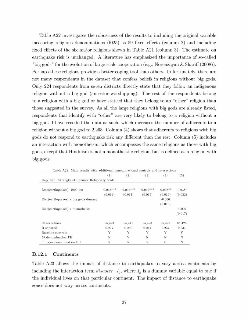
Table A22 investigates the robustness of the results to including the original variable

measuring religious denominations (f025) as 59 fixed effects (column 2) and including

fixed effects of the six major religions shown in Table A21 (column 3). The estimate on

earthquake risk is unchanged. A literature has emphasized the importance of so-called

"big gods" for the evolution of large-scale cooperation (e.g., Norenzayan & Shariff (2008)).

Perhaps these religions provide a better coping tool than others. Unfortunately, there are

not many respondents in the dataset that confess beliefs in religions without big gods.

Only 224 respondents from seven districts directly state that they follow an indigenous

religion without a big god (ancestor worshipping). The rest of the respondents belong

to a religion with a big god or have stateed that they belong to an “other”religion than

those suggested in the survey. As all the large religions with big gods are already listed,

respondents that identify with “other”are very likely to belong to a religion without a

big god. I have recoded the data as such, which increases the number of adherents to a

religion without a big god to 2,268. Column (4) shows that adherents to religions with big

gods do not respond to earthquake risk any different than the rest. Column (5) includes

an interaction with monotheism, which encompasses the same religions as those with big

gods, except that Hinduism is not a monotheistic religion, but is defined as a religion with

big gods.

Table A22. Main results with additional denominational controls and interactions

(1) (2) (3) (4) (5)

Dep. var.: Strength of Intrinsic Religiosity Scale

Dist(earthquakes), 1000 km -0.043*** -0.045*** -0.040*** -0.038** -0.038*

(0.014) (0.014) (0.015) (0.019) (0.022)

Dist(earthquakes) x big gods dummy -0.006

(0.016)

Dist(earthquakes) x monotheism -0.007

(0.017)

Observations 85,423 85,411 85,423 85,423 85,423

R-squared 0.237 0.250 0.241 0.237 0.237

Baseline controls Y Y Y Y Y

59 denomination FE N Y N N N

6 major denomination FE N N Y N N

B.12.1 Continents

Table A23 allows the impact of distance to earthquakes to vary across continents by

including the interaction term disaster · Ig, where Ig is a dummy variable equal to one ifthe individual lives on that particular continent. The impact of distance to earthquake

zones does not vary across continents.

27

Table A23. Main results across continents

(1) (2) (3) (4) (5) (6)

Dep. var.: Strength of Intrinsic Religiosity Scale

Dist(earthquakes), 1000 km -0.063*** -0.067*** -0.046*** -0.066*** -0.069*** -0.067***

(0.016) (0.021) (0.016) (0.018) (0.019) (0.017)

Dist(earthquakes) X America 0.016

(0.032)

Dist(earthquakes) X Europe -0.062

(0.044)

Dist(earthquakes) X Asia 0.011

(0.049)

Dist(earthquakes) X Africa 0.031

(0.029)

Dist(earthquakes) X Oceania 0.051

(0.048)

Observations 104,040 104,040 104,040 104,040 104,040 104,040

R-squared 0.325 0.325 0.326 0.325 0.325 0.325

Baseline controls Y Y Y Y Y Y

Districts 591 591 591 591 591 591

Districts in group 97 287 145 53 9

Notes. The table replicates column (8) of Panel A of Table 2, including interaction terms between

earthquake risk and continents. All columns include both variables in the interaction term separately.

B.13 Additional disasters

The data on tropical storm intensity zones are based on the probability of occurrence of

storms falling within five wind speed categories of the Saffi r-Simpson Hurricane Scale.61

The five wind speed categories are: 1) 118-153 km/h, 2) 154-177 km/h, 3) 178-209 km/h,

4) 210-249 km/h, and 5) 250+ km/h. The Storm Intensity Zone layer shows areas where

each of these wind speed categories has a 10% probability of occurring within the next

10 years. For each district, the distance to storm intensity zones 2 or above is calculated.

Storm intensity zones 2 or above are depicted in Figure A4 below as the dark blue areas.

The data on volcanic eruption intensity zones measure the density of volcanic eruptions

based on the explosivity index for each eruption and the time period of the eruption.

Eruption information is spread to 100 km beyond point source to indicate areas that

could be affected by volcanic emissions or ground shaking. The source of the data is

worldwide historical volcanic eruptions occurring within the last 10,000 years (to 2002)

from Siebert & Simkin (2002).62 The volcanic eruptions were rated using the Volcanic

Explosivity Index (VEI), which is a simple 0-to-6 index of increasing explosivity, with each

successive integer representing about an order of magnitude increase. For each district,

61Available online at U.S. Geological Survey: http://www.usgs.gov/.62The data were digitalized by the Smithsonian Institution’s Global Volcanism Program,

http://www.volcano.si.edu/index.cfm.

28

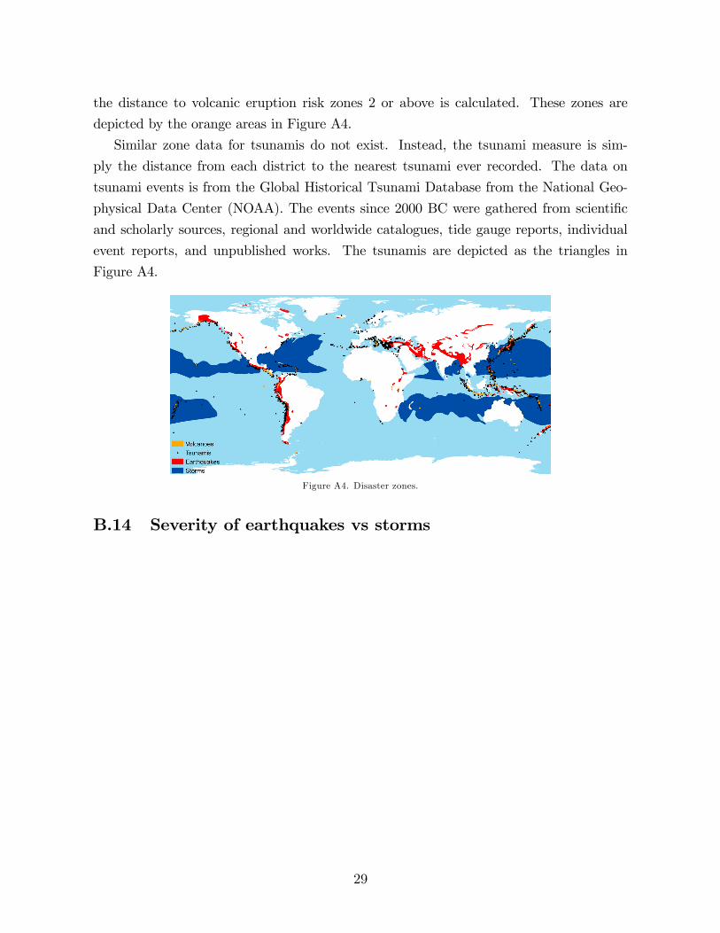
the distance to volcanic eruption risk zones 2 or above is calculated. These zones are

depicted by the orange areas in Figure A4.

Similar zone data for tsunamis do not exist. Instead, the tsunami measure is sim-

ply the distance from each district to the nearest tsunami ever recorded. The data on

tsunami events is from the Global Historical Tsunami Database from the National Geo-

physical Data Center (NOAA). The events since 2000 BC were gathered from scientific

and scholarly sources, regional and worldwide catalogues, tide gauge reports, individual

event reports, and unpublished works. The tsunamis are depicted as the triangles in

Figure A4.

Figure A4. Disaster zones.

B.14 Severity of earthquakes vs storms

29

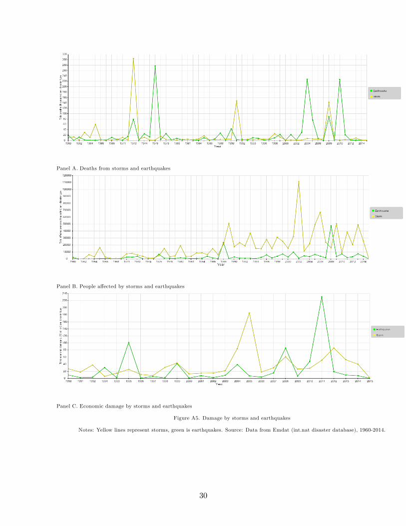
Panel A. Deaths from storms and earthquakes

Panel B. People affected by storms and earthquakes

Panel C. Economic damage by storms and earthquakes

Figure A5. Damage by storms and earthquakes

Notes: Yellow lines represent storms, green is earthquakes. Source: Data from Emdat (int.nat disaster database), 1960-2014.

30

B.15 Heterogeneity by development

Table A24 replicates column (8) of Panel A in Table 2, checking whether the effect of

earthquake risk differs across individuals’level of income or education and whether the

respondent works as an agricultural worker or is unemployed. The two latter variables

are based on variables x036 and x028. Columns (1), (3), (5) and (7) add interactions

between earthquake risk and individual income, education, status as agricultural worker,

and employment status. Columns (2) and (4) add interactions with the individual deciles

of the income measure and the different categories of education. The impact of earthquake

risk does not vary systematically within different income or education levels.

Earthquake risk does increase religiosity significantly more for the unemployed (column

7), even controlling for the ten income fixed effects (column 8). The literature on religious

coping finds both dampening effects of income (e.g., Gurin et al. (1960)) and no effects

(e.g., Carl Pieper et al. (1992)). On the other hand, the literature on religious coping

agrees that individuals with fewer coping alternatives in general should be more inclined

to use religion for coping. One major alternative is social networks to turn to in times

of need (e.g., Pargament (2001)). Thus, the finding that unemployed individuals respond

more to earthquakes with increased believing, even conditioning on income, is consistent

with the religious coping literature.

Table A25 aggregates the same development measures up to the district level and

include the corresponding interactions with district-level development, controlling for in-

dividual level income in odd columns. Two additional measures that are only available

at the district-level are added: Light density at night and population density. Columns

(13) and (14) include an interaction between earthquake risk and the size of the district

area that the individual was interviewed in. This is meant as a test of selection in the

cross-section analysis; if the results were driven by atheists moving out of high-risk areas,

this effect should be larger for smaller districts, where moving is more likely to mean

moving out of the district. If anything, the opposite seems to be the case; earthquake risk

increases religiosity slightly more for larger districts.

31

Table A24. Main results with interactions with individual level development

(1) (2) (3) (4) (5) (6) (7) (8)

Dependent variable: Strength of Intrinsic Religiosity Scale

Measure of development Inc Inc Edu Edu Agri Agri Unempl Unempl

Dist(earthq), 1000km -0.048*** -0.061*** -0.053*** -0.046*** -0.059*** -0.048***

(0.017) (0.018) (0.014) (0.014) (0.016) (0.015)

Dist(earthq) x development -0.001 -0.001 -0.002 -0.002 -0.036*** -0.026***

(0.002) (0.001) (0.011) (0.011) (0.008) (0.007)

Dist(earthq) x dev1 -0.053*** -0.053***

(0.016) (0.018)

Dist(earthq) x dev2 -0.042** -0.055***

(0.016) (0.018)

Dist(earthq) x dev3 -0.052*** -0.051***

(0.015) (0.018)

Dist(earthq) x dev4 -0.056*** -0.077***

(0.016) (0.018)

Dist(earthq) x dev5 -0.054*** -0.073***

(0.017) (0.021)

Dist(earthq) x dev6 -0.047*** -0.072***

(0.016) (0.017)

Dist(earthq) x dev7 -0.053*** -0.051***

(0.017) (0.018)

Dist(earthq) x dev8 -0.038** -0.068***

(0.016) (0.018)

Dist(earthq) x dev9 -0.071***

(0.022)

Dist(earthq) x dev10 -0.059***

(0.023)

Observations 71,376 71,376 98,278 98,278 76,464 67,589 101,045 68,569

R-squared 0.310 0.310 0.329 0.330 0.311 0.310 0.330 0.317

Baseline controls Y Y Y Y Y Y Y Y

Development Inc Inc Edu Edu Agri Agri Unempl Unempl

Income FE N N N N N Y N Y

Notes. The table replicates column (8) of Panel A of Table 2, allowing for interactions with development. dev1 refers to

income decile 1 or educational level 1 (inadequately completed elementary education), dev2 refers to income decile 2 or

educational level 2 (completed compulsory elementary education), dev3 refers to income decile 3 or educational level 3

(incomplete secondary school, technical), dev4 refers to income decile 4 or educational level 4 (complete secondary school,

technical), dev5 refers to income decile 5 or educational level 5 (incomplete secondary school, university), dev6 refers to

income decile 6 or educational level 6 (complete secondary school, university), dev7 refers to income decile 7 or educational

level 7 (some university without degree), dev8 refers to income decile 8 or educational level 8 (university with degree), dev9

and dev10 are the last income deciles. Both variables in interaction terms are included separately.

32

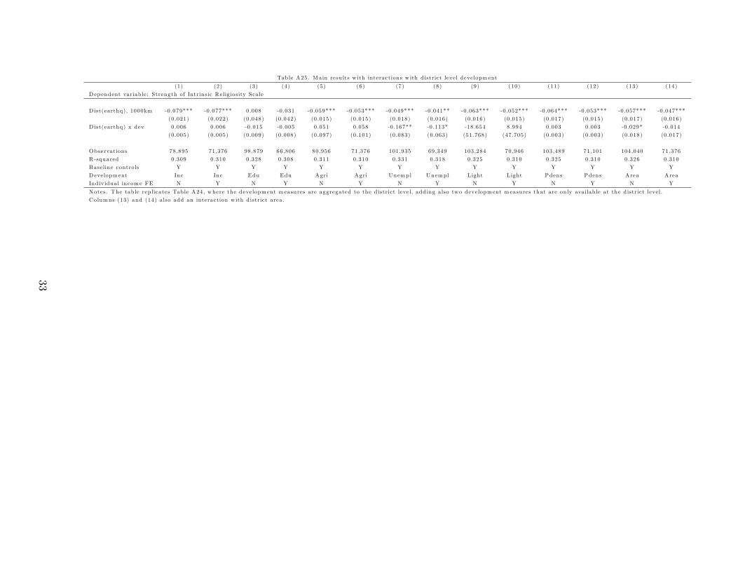
Table A25. M ain resu lts w ith interactions w ith d istrict level developm ent

(1) (2) (3) (4) (5) (6) (7) (8) (9) (10) (11) (12) (13) (14)

Dep endent variab le: Strength of Intrinsic Relig iosity Scale

D ist(earthq), 1000km -0.079*** -0 .077*** 0.008 -0 .031 -0 .059*** -0 .053*** -0 .049*** -0 .041** -0 .063*** -0 .052*** -0 .064*** -0 .053*** -0 .057*** -0 .047***

(0.021) (0 .022) (0 .048) (0 .042) (0 .015) (0 .015) (0 .018) (0 .016) (0 .016) (0 .015) (0 .017) (0 .015) (0 .017) (0 .016)

D ist(earthq) x dev 0.006 0.006 -0 .015 -0 .005 0.051 0.058 -0 .167** -0 .113* -18.654 8.994 0.003 0.003 -0 .029* -0 .014

(0.005) (0 .005) (0 .009) (0 .008) (0 .097) (0 .101) (0 .083) (0 .063) (51.768) (47.705) (0 .003) (0 .003) (0 .018) (0 .017)

Observations 78,895 71,376 98,879 66,806 80,956 71,376 101,935 69,349 103,284 70,946 103,489 71,101 104,040 71,376

R -squared 0.309 0.310 0.328 0.308 0.311 0.310 0.331 0.318 0.325 0.310 0.325 0.310 0.326 0.310

Baseline contro ls Y Y Y Y Y Y Y Y Y Y Y Y Y Y

Developm ent Inc Inc Edu Edu Agri Agri Unempl Unempl L ight L ight Pdens Pdens Area Area

Indiv idual incom e FE N Y N Y N Y N Y N Y N Y N Y

Notes. The tab le rep licates Table A24, where the developm ent m easures are aggregated to the d istrict level, add ing also two development m easures that are on ly availab le at the d istrict level.

Columns (13) and (14) also add an interaction w ith d istrict area.

33

B.16 Google searches on religion

An alternative measure of religiosity that is not based on surveys is Google searches for

religious terms. Google trends provides data on the share of total Google searches on

specified search terms for various geographic units. These data are comparable across

societies where the entire population have access to the internet. This is close to being

the case for current US states. Table A26 below shows the relation between earthquake

risk, defined throughout Section 3, and the frequency of various searches on religious

terms as a share of total Google searches per US state. The particular search terms are

"God", "church", "Jesus", "Bible", and "pray". A simple search on some of these search

terms includes searches that have nothing to do with religion. For instance "God of war"

is a computer game, Justin Beaber has a song called "Pray", and "Eat, Pray, Love" is a

romantic comedy. I remove these from the searches.

Table A26. OLS of google searches on religious terms on earthquake risk across US states

(1) (2) (3) (4) (5) (6) (7) (8) (9)

Dep. var.: Google searches of religious terms as a share of total google searches

Search term god god god god god church bible jesus pray

Dist(earthq), 1000 km -0.022 -0.217*** -0.218*** -0.215*** -0.180*** -0.104 -0.248*** -0.159*** -0.179**

(0.073) (0.068) (0.068) (0.068) (0.060) (0.082) (0.083) (0.056) (0.065)

Dist(ocean), 1000 km 0.030 0.033 0.025 0.101** 0.058 0.027 -0.040

(0.029) (0.033) (0.033) (0.041) (0.050) (0.025) (0.044)

Absolute latitude -0.001 0.000 0.001 0.002 -0.002 -0.007

(0.002) (0.003) (0.002) (0.003) (0.002) (0.006)

GSP per capita 2010 -0.003** -0.004** -0.005** -0.003** -0.005

(0.001) (0.002) (0.002) (0.001) (0.003)

Observations 50 50 50 50 50 50 50 50 34

R-squared 0.001 0.717 0.719 0.722 0.755 0.768 0.774 0.797 0.774

Region fixed effects N Y Y Y Y Y Y Y Y

34

C Additional results for event studyThis section investigates the robustness of the main results in Panel B of Table 4. Overall,

intrinsic religiosity (importance of God and religious person) increases with earthquakes,

while extrinsic religiosity (attendance at religious services) does not. This is consistent

with the religious coping hypothesis, and inconsistent with a purely economic explana-

tions, where individuals go to church for aid. Results using the share of religious persons

are less robust to changes, while the average importance of God in a district is robust to

most changes. This is not surprising, since whether or not individuals regard themselves

as religious involves a much larger change than how important they rank God on a scale

from zero to ten. Thus, the test using the share of religious persons is a more demanding

one.

C.1 Data on earthquake events

Downloadable from the Comprehensive Earthquake Catalogue: earthquake.usgs.gov/monitoring/anss/.

The U.S. Geological Survey provides the best available estimate of an earthquake’s mag-

nitude. Each method to measure magnitudes works over a limited range of magnitudes.

Some methods are based on body waves (which travel deep within the structure of the

earth) and some are based on surface waves (which primarily travel along the upper-

most layers). All of the methods are designed to agree well over the range of magnitudes

where they are reliable. Earthquake magnitude is a logarithmic measure of earthquake

size, which means that the shaking will be 10 times as large during a magnitude 6 earth-

quake as during a magnitude 5 earthquake. The total amount of energy released by the

earthquake, however, goes up by a factor of 32.

The number of earthquakes of all magnitudes in the data increases up until 1973 and

the number of earthquakes of magnitudes below 5 increases over the entire period. While

the number of earthquakes has not increased in reality, the implication is that earthquake

detection technology must have improved over time. There has been no trend in the

number of earthquakes of magnitude 5 or above since 1973. On the USGS website it

says: “We may not rapidly locate earthquakes smaller than 5.0 outside the US unless

they have caused significant damage or are widely felt. Earthquakes this small rarely

cause significant damage. At times, some other agency may report an earthquake with

a larger magnitude than what we compute from our data, especially for non-US events

near magnitude 5.0. If our magnitude for the event is less than magnitude 5.0, we may

not issue a rapid report for it.”

Years since the last earthquake is coded as 100 in districts that did not experience an

35

earthquake since 1973. The results do not depend on this threshold.

C.2 Varying cut-off levels

The main analysis defines a district as being hit by an earthquake if the earthquake hit

within 100 km of the district borders. Panels A and B of Table A26 show that the results

are robust to varying the cut-off level from 0 to 200 km in increments of 50 km when

using importance of God as the measure of religiosity. Panel C shows that the results

using the share of religious persons are less robust to choice of cut-off levels. Part of

the sensitivity seems to be due to a few outliers (removed in Panel D). The finding that

attendance rates are unaffected by earthquakes is robust to different cut-off levels (Panel

E). But when excluding outliers, churchgoing seems to fall with earthquakes in districts

otherwise rarely hit for earthquakes that hit within district borders (cut off zero).

The reason for the varying number of observations is that district-years are excluded if

an earthquake hit in the year of the interview, discussed in the main text. Note that this

restriction also happens to exclude all districts where an earthquake hit within district

borders for all cut-off levels 50-200.

36

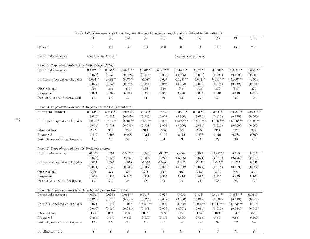
Table A27. Main results with varying cut-off levels for when an earthquake is defined to hit a district

(1) (2) (3) (4) (5) (6) (7) (8) (9) (10)

Cut-off 0 50 100 150 200 0 50 100 150 200

Earthquake measure: Earthquake dummy Number earthquakes

Panel A. Dependent variable: D. Importance of God

Earthquake measure 0.107*** 0.089** 0.093*** 0.070*** 0.067*** 0.107*** 0.074** 0.058** 0.044*** 0.030***

(0.035) (0.035) (0.028) (0.022) (0.018) (0.035) (0.033) (0.021) (0.009) (0.009)

Earthq x Frequent earthquakes -0.094** -0.081** -0.073** -0.027 0.027 -0.103*** -0.083** -0.053*** -0.040*** -0.019

(0.037) (0.035) (0.029) (0.024) (0.080) (0.033) (0.032) (0.019) (0.012) (0.014)

Observations 370 353 350 335 326 370 353 350 335 326

R-squared 0.341 0.336 0.338 0.319 0.317 0.340 0.334 0.333 0.316 0.310

District-years with earthquake 13 25 33 41 46 13 25 33 41 46

Panel B. Dependent variable: D. Importance of God (no outliers)

Earthquake measure 0.092*** 0.054*** 0.066*** 0.045* 0.042* 0.092*** 0.046*** 0.052*** 0.033*** 0.023***

(0.030) (0.015) (0.015) (0.026) (0.024) (0.030) (0.013) (0.011) (0.010) (0.008)

Earthq x Frequent earthquakes -0.080** -0.047** -0.039** -0.047** 0.007 -0.089*** -0.058*** -0.047*** -0.029*** -0.021**

(0.034) (0.018) (0.016) (0.018) (0.006) (0.029) (0.014) (0.011) (0.009) (0.009)

Observations 352 337 334 319 306 352 335 331 320 307

R-squared 0.412 0.405 0.408 0.391 0.402 0.412 0.406 0.406 0.388 0.399

District-years with earthquake 13 24 31 40 44 13 24 29 40 44

Panel C. Dependent variable: D. Religious person

Earthquake measure -0.002 0.031 0.062** 0.040 -0.002 -0.002 0.024 0.044*** 0.028 0.011

(0.036) (0.033) (0.027) (0.054) (0.028) (0.036) (0.021) (0.014) (0.026) (0.019)

Earthq x Frequent earthquakes 0.011 0.007 -0.058 -0.079 0.069+ 0.007 -0.028 -0.046** -0.027 0.021

(0.041) (0.038) (0.041) (0.067) (0.042) (0.038) (0.024) (0.018) (0.029) (0.022)

Observations 390 373 370 355 345 390 373 370 355 345

R-squared 0.414 0.416 0.417 0.411 0.397 0.414 0.415 0.417 0.410 0.400

District-years with earthquake 14 25 33 38 42 14 25 33 38 42

Panel D. Dependent variable: D. Religious person (no outliers)

Earthquake measure -0.023 0.026+ 0.064*** 0.083** 0.028 -0.023 0.023* 0.046*** 0.053*** 0.031**

(0.036) (0.016) (0.014) (0.035) (0.028) (0.036) (0.012) (0.007) (0.010) (0.013)

Earthq x Frequent earthquakes 0.031 0.014 -0.046 -0.089*** 0.039 0.028 -0.030** -0.049*** -0.053*** 0.015

(0.039) (0.028) (0.034) (0.031) (0.059) (0.037) (0.014) (0.012) (0.014) (0.018)

Observations 374 356 351 337 329 374 354 351 338 326

R-squared 0.495 0.514 0.517 0.523 0.498 0.495 0.515 0.517 0.517 0.500

District-years with earthquake 14 25 32 36 41 14 25 32 37 39

Baseline controls Y Y Y Y Y Y Y Y Y Y

37

Table A27 cont. Main results with varying cut-off levels for when an earthquake is defined to hit a district

(1) (2) (3) (4) (5) (6) (7) (8) (9) (10)

Cut-off 0 50 100 150 200 0 50 100 150 200

Earthquake measure: Earthquake dummy Number earthquakes

Panel E. Dependent variable: D. attend religious services

Earthquake measure -0.061 -0.008 0.028 0.025 0.044 -0.063 -0.003 0.021 0.016 0.008

(0.066) (0.031) (0.046) (0.055) (0.035) (0.066) (0.020) (0.023) (0.028) (0.017)

Earthq x Frequent earthquakes 0.129 0.052 0.012 0.053 0.286*** 0.078 0.015 -0.020 -0.004 0.029

(0.102) (0.044) (0.077) (0.119) (0.068) (0.074) (0.023) (0.026) (0.039) (0.036)

Observations 404 387 384 369 357 404 387 384 369 357

R-squared 0.517 0.509 0.516 0.509 0.531 0.515 0.508 0.515 0.507 0.517

District-years with earthquake 14 25 33 38 42 14 25 33 38 42

Panel F. Dependent variable: D. attend religious services (no outliers)

Earthquake measure -0.121*** -0.026 0.008 0.003 0.014 -0.121*** -0.010 0.006 0.008 0.006

(0.015) (0.019) (0.012) (0.033) (0.010) (0.015) (0.013) (0.013) (0.018) (0.005)

Earthq x Frequent earthquakes 0.140*** 0.056** -0.014 -0.008 0.070*** 0.129*** 0.022* -0.005 -0.020 0.093**

(0.015) (0.020) (0.019) (0.038) (0.015) (0.012) (0.011) (0.010) (0.017) (0.034)

Observations 386 370 367 351 341 386 370 368 350 339

R-squared 0.549 0.527 0.529 0.531 0.544 0.549 0.525 0.530 0.529 0.547

District-years with earthquake 12 22 29 34 40 12 22 30 33 37

Baseline controls Y Y Y Y Y Y Y Y Y Y

Notes. OLS estimates. The dependent variable is the change in the district average of importance of God in Panels A and B, district share of religious

persons in Panels C and D, and average attendance at religious services in Panels E and F. Earthquakes are measured with the dummy variable in columns

(1)-(5) and the number of earthquakes in columns (6)-(10). Outliers detected based on Cooks D>1.

38

C.3 Simple figure

Figure A6 Change in religiosity by earthquake or not for window of 6 years or less

Notes. Lines show 90 pct confidence bounds.The sample is restricted to districts measured 6 years or less apart

39

C.4 Controls

C.4.1 Results with fewer controls

Table A28. Main results adding controls consecutively

(1) (2) (3) (4) (5) (6) (7) (8) (9) (10)

Dependent variable: Avg Diff Diff Diff Diff Diff Diff Diff Diff Diff

Panel A. Importance of God

Earthquake dummy 0.17** 0.04 0.08* 0.07** 0.09** 0.08** 0.09*** 0.09*** 0.09*** 0.09***

(0.07) (0.03) (0.04) (0.03) (0.03) (0.03) (0.03) (0.03) (0.03) (0.03)

Earthq x Frequent earthq -0.27*** -0.07 -0.13** -0.11** -0.12*** -0.12*** -0.09** -0.09*** -0.07** -0.07**

(0.08) (0.05) (0.06) (0.04) (0.04) (0.04) (0.03) (0.03) (0.03) (0.03)

Observations 641 366 362 361 361 361 361 357 353 350

Districts 308 242 238 238 238 238 238 236 238 236

R-squared 0.04 0.01 0.16 0.26 0.26 0.27 0.32 0.32 0.34 0.34

Mean dep var 0.683 0.000 0.000 0.000 0.000 0.000 0.000 0.001 0.003 0.003

Panel B: Religious persons

Earthquake dummy 0.12* 0.01 0.03 0.04 0.05* 0.05* 0.06** 0.06** 0.06** 0.06**

(0.06) (0.04) (0.03) (0.03) (0.03) (0.03) (0.03) (0.03) (0.03) (0.03)

Earthq x Frequent earthq -0.19*** -0.02 -0.11*** -0.09** -0.10*** -0.10*** -0.09** -0.09** -0.06 -0.06

(0.07) (0.05) (0.03) (0.04) (0.03) (0.03) (0.04) (0.04) (0.04) (0.04)

Observations 630 386 382 381 381 381 381 377 373 370

Districts 289 256 252 252 252 252 252 250 252 250

R-squared 0.02 0.00 0.37 0.39 0.39 0.39 0.41 0.41 0.42 0.42

Mean dep var 0.686 -0.02 -0.02 -0.02 -0.02 -0.02 -0.02 -0.02 -0.02 -0.02

Panel C: Attendance at religious services

Earthquake dummy 0.13*** -0.08*** 0.00 0.01 0.02 0.02 0.03 0.03 0.02 0.02

(0.04) (0.03) (0.04) (0.04) (0.04) (0.04) (0.05) (0.04) (0.05) (0.04)

Earthq x Frequent earthq -0.21** 0.09 -0.03 -0.02 -0.03 -0.03 -0.01 -0.01 0.01 0.01

(0.08) (0.05) (0.08) (0.07) (0.08) (0.08) (0.08) (0.07) (0.08) (0.08)

Observations 668 399 396 395 395 395 395 391 387 384

Districts 296 269 266 266 266 266 266 264 266 264

R-squared 0.03 0.02 0.43 0.48 0.48 0.48 0.50 0.50 0.51 0.51

Mean dep var 0.437 0.003 0.003 0.003 0.003 0.003 0.003 0.003 0.005 0.004

Country fixed effects N N Y Y Y Y Y Y Y Y

Year fixed effects N N N Y Y Y Y Y Y Y

Years since last eq N N N N Y Y Y Y Y Y

Years between waves N N N N N Y Y Y Y Y

Country-specific trends N N N N N N Y N Y N

Country-by-year FE N N N N N N N Y N Y

Individual level controls N N N N N N N N Y Y

Notes. The dependent variable is based on the degree of importance of God in Panel A, religious persons in panel B, and the

attendance at religious services in panel C. The dependent variable is in levels in column (1) and in changes in columns (2)-(10).

Standard errors are clustered at the country level. Asterisks ***, **, *, and + indicate significance at the 1, 5, 10%, and 15% level,

respectively.

40

C.4.2 Additional controls

Table A29 adds ten income fixed effects. The sample is restricted to the sample with

information on individual income in uneven columns, while ten income fixed effects are

added to the set of baseline controls in even columns. Table A30 adds the same additional

measures of cultural values as added in Table A14. The results are unaltered.

41

Table A29. Main results with individual income fixed effects

(1) (2) (3) (4) (5) (6) (7) (8) (9) (10) (11) (12)

Earthquakes measure: Earthquake dummy Number earthquakes Earthquake dummy Number earthquakes Earthquake dummy Number earthquakes

Dependent variable: D.Importance of God D.Religious person D.Attend services

Earthquake measure 0.087*** 0.084*** 0.054** 0.053*** 0.065** 0.054* 0.045*** 0.039*** 0.016 0.010 0.014 0.011

(0.029) (0.026) (0.020) (0.018) (0.027) (0.027) (0.013) (0.012) (0.045) (0.045) (0.022) (0.022)

Earthq x Frequent earthq -0.068** -0.074** -0.049** -0.052*** -0.061 -0.078* -0.047** -0.048** 0.022 0.022 -0.014 -0.013

(0.029) (0.027) (0.018) (0.017) (0.041) (0.039) (0.018) (0.018) (0.076) (0.070) (0.024) (0.023)

Observations 276 276 276 276 296 296 296 296 310 310 310 310

R-squared 0.349 0.282 0.344 0.278 0.435 0.388 0.435 0.389 0.527 0.442 0.526 0.442

Income FE N Y N Y N Y N Y N Y N Y

Baseline controls Y Y Y Y Y Y Y Y Y Y Y Y

42

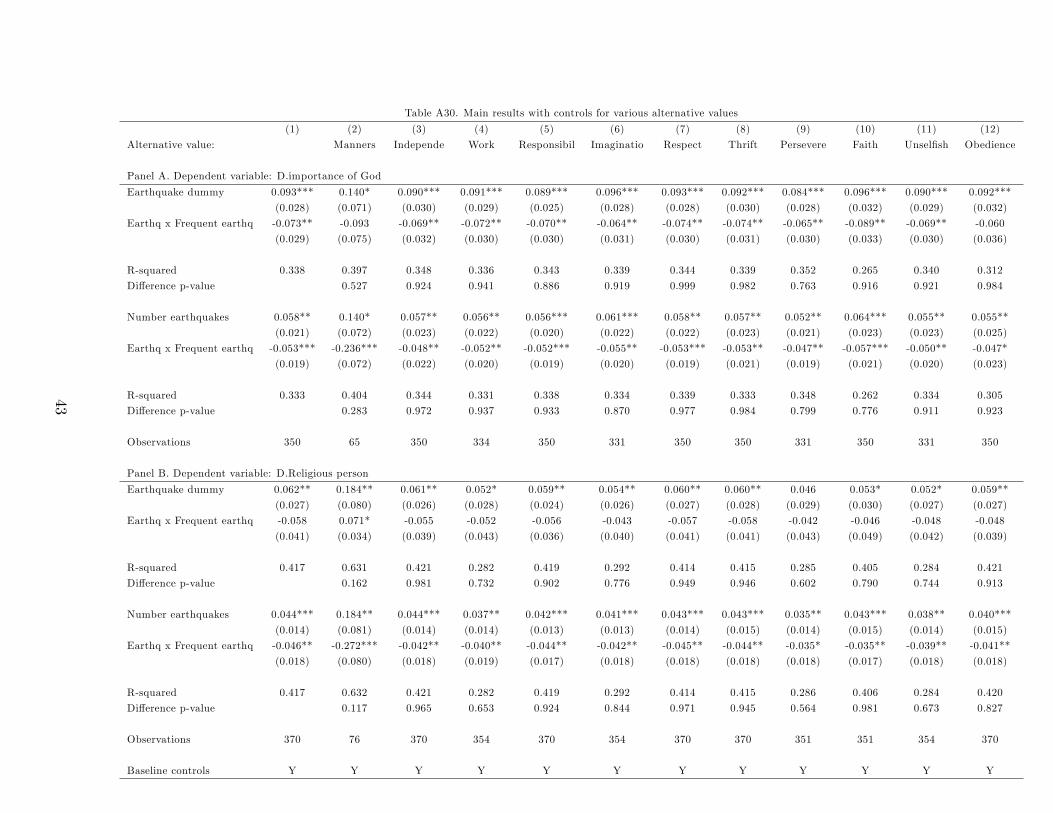
Table A30. Main results with controls for various alternative values

(1) (2) (3) (4) (5) (6) (7) (8) (9) (10) (11) (12)

Alternative value: Manners Independe Work Responsibil Imaginatio Respect Thrift Persevere Faith Unselfish Obedience

Panel A. Dependent variable: D.importance of God

Earthquake dummy 0.093*** 0.140* 0.090*** 0.091*** 0.089*** 0.096*** 0.093*** 0.092*** 0.084*** 0.096*** 0.090*** 0.092***

(0.028) (0.071) (0.030) (0.029) (0.025) (0.028) (0.028) (0.030) (0.028) (0.032) (0.029) (0.032)

Earthq x Frequent earthq -0.073** -0.093 -0.069** -0.072** -0.070** -0.064** -0.074** -0.074** -0.065** -0.089** -0.069** -0.060

(0.029) (0.075) (0.032) (0.030) (0.030) (0.031) (0.030) (0.031) (0.030) (0.033) (0.030) (0.036)

R-squared 0.338 0.397 0.348 0.336 0.343 0.339 0.344 0.339 0.352 0.265 0.340 0.312

Difference p-value 0.527 0.924 0.941 0.886 0.919 0.999 0.982 0.763 0.916 0.921 0.984

Number earthquakes 0.058** 0.140* 0.057** 0.056** 0.056*** 0.061*** 0.058** 0.057** 0.052** 0.064*** 0.055** 0.055**

(0.021) (0.072) (0.023) (0.022) (0.020) (0.022) (0.022) (0.023) (0.021) (0.023) (0.023) (0.025)

Earthq x Frequent earthq -0.053*** -0.236*** -0.048** -0.052** -0.052*** -0.055** -0.053*** -0.053** -0.047** -0.057*** -0.050** -0.047*

(0.019) (0.072) (0.022) (0.020) (0.019) (0.020) (0.019) (0.021) (0.019) (0.021) (0.020) (0.023)

R-squared 0.333 0.404 0.344 0.331 0.338 0.334 0.339 0.333 0.348 0.262 0.334 0.305

Difference p-value 0.283 0.972 0.937 0.933 0.870 0.977 0.984 0.799 0.776 0.911 0.923

Observations 350 65 350 334 350 331 350 350 331 350 331 350

Panel B. Dependent variable: D.Religious person

Earthquake dummy 0.062** 0.184** 0.061** 0.052* 0.059** 0.054** 0.060** 0.060** 0.046 0.053* 0.052* 0.059**

(0.027) (0.080) (0.026) (0.028) (0.024) (0.026) (0.027) (0.028) (0.029) (0.030) (0.027) (0.027)

Earthq x Frequent earthq -0.058 0.071* -0.055 -0.052 -0.056 -0.043 -0.057 -0.058 -0.042 -0.046 -0.048 -0.048

(0.041) (0.034) (0.039) (0.043) (0.036) (0.040) (0.041) (0.041) (0.043) (0.049) (0.042) (0.039)

R-squared 0.417 0.631 0.421 0.282 0.419 0.292 0.414 0.415 0.285 0.405 0.284 0.421

Difference p-value 0.162 0.981 0.732 0.902 0.776 0.949 0.946 0.602 0.790 0.744 0.913

Number earthquakes 0.044*** 0.184** 0.044*** 0.037** 0.042*** 0.041*** 0.043*** 0.043*** 0.035** 0.043*** 0.038** 0.040***

(0.014) (0.081) (0.014) (0.014) (0.013) (0.013) (0.014) (0.015) (0.014) (0.015) (0.014) (0.015)

Earthq x Frequent earthq -0.046** -0.272*** -0.042** -0.040** -0.044** -0.042** -0.045** -0.044** -0.035* -0.035** -0.039** -0.041**

(0.018) (0.080) (0.018) (0.019) (0.017) (0.018) (0.018) (0.018) (0.018) (0.017) (0.018) (0.018)

R-squared 0.417 0.632 0.421 0.282 0.419 0.292 0.414 0.415 0.286 0.406 0.284 0.420

Difference p-value 0.117 0.965 0.653 0.924 0.844 0.971 0.945 0.564 0.981 0.673 0.827

Observations 370 76 370 354 370 354 370 370 351 351 354 370

Baseline controls Y Y Y Y Y Y Y Y Y Y Y Y

43

Table A30 cont. Main results with controls for various alternative values

(1) (2) (3) (4) (5) (6) (7) (8) (9) (10) (11) (12)

Alternative value: Manners Independence Work Responsibility Imagination Respect Thrift Perseverence Faith Unselfish Obedience

Panel C. Dependent variable: D.attend religious services

Earthquake dummy 0.024 -0.022 0.024 0.018 0.020 0.019 0.024 0.023 0.012 0.033 0.017 0.023

(0.044) (0.033) (0.046) (0.043) (0.049) (0.044) (0.044) (0.044) (0.042) (0.042) (0.044) (0.045)

Earthq x Frequent earthq 0.014 0.054 0.013 0.018 0.017 0.025 0.013 0.013 0.026 0.005 0.020 0.023

(0.077) (0.041) (0.078) (0.075) (0.085) (0.078) (0.076) (0.077) (0.074) (0.068) (0.076) (0.082)

R-squared 0.513 0.270 0.503 0.527 0.503 0.517 0.511 0.514 0.542 0.388 0.525 0.504

Difference p-value 0.201 0.997 0.895 0.941 0.917 0.997 0.991 0.790 0.831 0.888 0.981

Number earthq 0.017 -0.022 0.018 0.014 0.015 0.016 0.018 0.017 0.011 0.026 0.013 0.015

(0.022) (0.033) (0.023) (0.022) (0.024) (0.022) (0.022) (0.022) (0.021) (0.022) (0.022) (0.023)

Earthq x Frequent earthq -0.018 -0.031 -0.016 -0.014 -0.016 -0.016 -0.018 -0.017 -0.010 -0.018 -0.013 -0.014

(0.025) (0.033) (0.026) (0.024) (0.027) (0.024) (0.024) (0.025) (0.023) (0.025) (0.024) (0.026)

R-squared 0.513 0.271 0.502 0.526 0.502 0.517 0.510 0.514 0.541 0.388 0.524 0.503

Difference p-value 0.267 0.997 0.862 0.935 0.942 0.985 0.972 0.742 0.695 0.835 0.906

Observations 384 76 384 368 384 368 384 384 365 365 368 384

Baseline controls Y Y Y Y Y Y Y Y Y Y Y Y

Notes. OLS estimates. The table replicates Panel B of Table 4 adding various additional values as controls. All are described by Table A14. "Difference p-value" indicates the

p-value of the test that the estimate on earthquakes in low risk districts equals the estimate in column (1).

44

Table A31 includes ethnicity fixed effects (variable x051).

Table A31. Main results with ethnicity fixed effects

(1) (2) (3) (4) (5) (6)

Dep. var.: D.impgod D.relpers D.service

Panel A. Earthquake dummy

Earthquake dummy 0.067** 0.055** 0.064 0.077 0.129 0.054

(0.029) (0.024) (0.060) (0.071) (0.076) (0.074)

R-squared 0.371 0.320 0.534 0.485 0.439 0.450

Panel B. Number earthquakes

Number earthquakes 0.017* 0.015** 0.032* 0.031 0.028 0.016

(0.010) (0.007) (0.017) (0.022) (0.025) (0.021)

R-squared 0.367 0.317 0.535 0.484 0.425 0.447

Observations 145 145 143 143 143 143

Baseline controls Y Y Y Y Y Y

Ethnicity fixed effects Y N Y N Y N

Notes. OLS estimates. The table replicates Panel B of Table 4 adding ethnicity fixed effects in odd columns.

Even columns exclude ethnic fixed effects on the sample restricted to that with information on ethnicity.

45

C.5 Comparison of the estimate sizes

C.5.1 Standardized beta coeffi cients

Table A32. Main results with standardized coeffi cients

(1) (2) (3) (4) (5) (6)

Dep. var. D.impgod D.rel_pers D.service D.impgod D.rel_pers D.service

Panel A. Baseline results

Earthquake dummy 0.226*** 0.109** 0.089 0.229*** 0.100** 0.116

(0.069) (0.044) (0.078) (0.073) (0.045) (0.087)

R-squared 0.335 0.414 0.509 0.335 0.424 0.398

P-value beta=.229 1 0.00723 0.204

Panel B. Allowing for differential effect depending on how frequent the district is hit

Earthquake dummy 0.276*** 0.127** 0.061 0.282*** 0.113** 0.093

(0.082) (0.055) (0.115) (0.089) (0.055) (0.123)

Earthquake dummy x Frequent earthq -0.172** -0.097 0.029 -0.177** -0.065 0.039

(0.068) (0.068) (0.159) (0.074) (0.063) (0.179)

R-squared 0.338 0.417 0.513 0.338 0.427 0.408

P-value beta=.282 1 0.00444 0.135

Observations 350 370 384 338 338 338

Baseline controls Y Y Y Y Y Y

Sample full full full same same same

C.5.2 Same sample

Table A33 replicates Table 4 to the sample across columns.

46

Table A33. Main results restricted to the same sample across columns

(1) (2) (3) (4) (5) (6) (7) (8) (9) (10) (11) (12)

Dependent variable D.impgod D.relpers D.service D.impgod D.relpers D.service

Earthquake measure: Earthquake dummy Number earthquakes

Panel A. Linear effects of earthquakes

Earthquake measure 0.077*** 0.074*** 0.049** 0.042** 0.043 0.039 0.077*** 0.074*** 0.049** 0.042** 0.043 0.039

(0.025) (0.023) (0.022) (0.020) (0.032) (0.040) (0.025) (0.023) (0.022) (0.020) (0.032) (0.040)

R-squared 0.335 0.305 0.424 0.425 0.398 0.417 0.335 0.305 0.424 0.425 0.398 0.417

Panel B. Allowing for differential effects depending on how frequent the district is hit

Earthquake measure 0.095*** 0.088*** 0.056** 0.053** 0.034 0.030 0.095*** 0.088*** 0.056** 0.053** 0.034 0.030

(0.030) (0.026) (0.027) (0.023) (0.045) (0.053) (0.030) (0.026) (0.027) (0.023) (0.045) (0.053)

Earthq x Frequent earthq -0.075** -0.062* -0.041 -0.043+ 0.018 0.058 -0.075** -0.062* -0.041 -0.043+ 0.018 0.058

(0.031) (0.033) (0.039) (0.029) (0.083) (0.095) (0.031) (0.033) (0.039) (0.029) (0.083) (0.095)

R-squared 0.338 0.307 0.427 0.428 0.408 0.430 0.338 0.307 0.427 0.428 0.408 0.430

Panel C. Placebo regressions

Earthquake measure w+1 -0.026 -0.016 0.027 0.027 -0.054 -0.052 -0.025 -0.016 0.018 0.018 -0.047 -0.042

(0.021) (0.026) (0.043) (0.049) (0.049) (0.047) (0.018) (0.021) (0.037) (0.042) (0.044) (0.041)

Earthq w+1 x Frequent earthq -0.016 -0.032 -0.004 -0.012 0.113+ 0.129** 0.016 0.009 -0.018 -0.016 0.034 0.033

(0.021) (0.028) (0.048) (0.055) (0.067) (0.058) (0.017) (0.021) (0.034) (0.040) (0.043) (0.042)

R-squared 0.319 0.290 0.425 0.426 0.410 0.431 0.319 0.290 0.425 0.425 0.409 0.428

Observations 338 312 338 312 338 312 338 312 338 312 338 312

Baseline controls Y Y Y Y Y Y Y Y Y Y Y Y

Education dummies N Y N Y N Y N Y N Y N Y

Districts 236 230 250 240 264 254 236 230 250 240 264 254

Countries 31 30 31 30 32 31 31 30 31 30 32 31

Number Fixed effects 46 50 47 49 48 50 46 50 47 49 48 50

Notes. The table replicates Table 4 on the restricted sample where all three religiosity measures are available.

47

C.6 Different measures of frequent earthquakes

In the main analysis, a district is defined as having been hit frequently by earthquakes

if the district lies in the top 95th percentile in terms of the number of earthquakes that

hit during the period for which there is comparable data on earthquake instances, 1973-

2014. This turns out to equal seven earthquakes or more. Columns (1)-(3), (5)-(7),

and (9)-(11) of Table A34 show that the results do not depend on the exact choice of

percentile, particularly when measuring religiosity along the intensive margin (importance

of God and attendance rates). Again the extensive margin (share of religious persons) is

somewhat less robust. The results are also robust to using instead a dummy equal to one

if the district is located within the earthquake zone 3 or 4 as defined in the cross-district

analysis (columns 4, 8, and 12).

48

Table A34. Main results with different high-frequency measures

(1) (2) (3) (4) (5) (6) (7) (8) (9) (10) (11) (12)

Dependent variable D.importance of God D.religious person D.Attend services

Panel A. Earthquake dummy

Earthquake dummy 0.131*** 0.093*** 0.078*** 0.098** 0.062 0.062** 0.052** 0.071*** 0.022 0.024 0.033 0.030

(0.046) (0.028) (0.024) (0.037) (0.050) (0.027) (0.022) (0.025) (0.091) (0.044) (0.031) (0.047)

Earthq x Frequent earthq -0.093+ -0.073** -0.045* -0.048 -0.031 -0.058 0.008 -0.041 0.016 0.014 0.038 0.011

(0.058) (0.029) (0.024) (0.042) (0.050) (0.041) (0.022) (0.030) (0.100) (0.077) (0.031) (0.064)

R-squared 0.342 0.338 0.335 0.338 0.416 0.417 0.414 0.415 0.509 0.513 0.509 0.509

Panel B. Number earthquakes

Number earthquakes 0.100** 0.058** 0.030** 0.058* 0.050+ 0.044*** 0.023*** 0.029* -0.003 0.017 0.014 0.006

(0.043) (0.021) (0.012) (0.030) (0.033) (0.014) (0.007) (0.016) (0.066) (0.022) (0.010) (0.018)

Earthq x Frequent earthq -0.088* -0.053*** -0.024* -0.044+ -0.038 -0.046** -0.006 -0.012 0.018 -0.018 0.004 0.015

(0.047) (0.019) (0.012) (0.030) (0.033) (0.018) (0.007) (0.016) (0.071) (0.025) (0.010) (0.020)

R-squared 0.337 0.333 0.326 0.331 0.416 0.417 0.413 0.414 0.509 0.513 0.508 0.509

Observations 350 350 350 350 370 370 370 370 384 384 384 384

High risk measure >=90 pct >=95 pct >=99 pct zone >=90 pct >=95 pct >=99 pct zone >=90 pct >=95 pct >=99 pct zone

Baseline controls Y Y Y Y Y Y Y Y Y Y Y Y

Notes. OLS estimates. The dependent variable is the change in the district aggregate of importance of God in columns (1)-(4), the change in the share of religious

persons in columns (5)-(8), and the change in average attendance rates in columns (9)-(12). Panel A measures earthquakes with a dummy equal to one if the district was hit

by one or more earthquakes. In Panel B, the earthquake measure is the actual number of earthquakes. Baseline controls are the same as those in Table 4.

49

C.7 Dynamics and period lengths

The main regressions exclude district-years measured more than 10 years apart. Figure

A7 shows the distribution of years between interviews in the samples where the three

different religiosity measures are non-missing.

0.1

.2.3

Den

sity

0 5 10 15 20Years in between interviews

0.1

.2.3

Den

sity

0 5 10 15 20Years in between interviews

0.1

.2.3

Den

sity

0 5 10 15 20Years in between interviews

Importance of God Religious person Services

Figure A7. Distribution of the number of years between interviews

50

Table A35. Main results with same window lengths

(1) (2) (3) (4)

Panel A. Dep var: Changes in importance of God

Earthquake dummy 0.19** 0.16* 0.22** 0.22**

(0.09) (0.08) (0.09) (0.08)

Earthq x Frequent earthq -0.18** -0.05 -0.07 -0.07**

(0.09) (0.10) (0.10) (0.02)

Observations 92 90 88 88

Districts 61 59 58 58

R-squared 0.07 0.36 0.40 0.40

Panel B. Dep var: Changes in religious person

Earthquake dummy -0.05 -0.00 0.04 0.04

(0.08) (0.12) (0.13) (0.07)

Earthq x Frequent earthq 0.15* 0.02 0.01 0.01

(0.08) (0.14) (0.14) (0.02)

Observations 93 91 89 89

Districts 61 59 58 58

R-squared 0.03 0.09 0.10 0.10

Panel C. Dep var: Changes in attendance rates

Earthquake dummy -0.07 -0.09 -0.09 -0.09***

(0.07) (0.08) (0.09) (0.02)

Earthq x Frequent earthq 0.12* 0.01 0.02 0.02*

(0.07) (0.10) (0.10) (0.01)

Observations 93 91 89 89

Districts 61 59 58 58

R-squared 0.02 0.10 0.08 0.08

(0.05)

Country and year FE N Y Y Y

Country-by-year FE N N Y Y

Clustered se at country level N N N Y

Notes. The dependent variable is changes in average importance of God

in Panel A, religious persons in panel B, and the attendance at religious

services in panel C. Years since last earthquake is included throughout.

Robust standard errors in columns (1)-(3). Standard errors are clustered

at the country level in columns (4). Asterisks ***, **, *, and + indicate

significance at the 1, 5, 10%, and 15% level, respectively.

51

Table A36 exploits the difference in period lengths in order to investigate the short-

term dynamics of the effect of earthquakes. The main analysis excludes districts with more

than 10 years in between interviews. Column (1) shows that the results are robust to using

the full sample of period lengths. Columns (2)-(9) narrows the window of observation more

as we move to the right in the table from 12 years or below to 5 years or below. The reason

for not reducing the window of observation further is that the interaction with "Frequent

earthquakes" cannot be estimated in this sample. The impact of earthquakes on intrinsic

religiosity increases when narrowing the window of observation, consistent with the idea

that the impact falls over time. Table A37 shows that this is not because the period length

depends on characteristics such as earthquakes, district-level average income, education,

age of the respondents, fraction males, or fraction married. The finding that attendance

rates are unaffected by earthquakes is robust to different period lengths (Panel C).

52

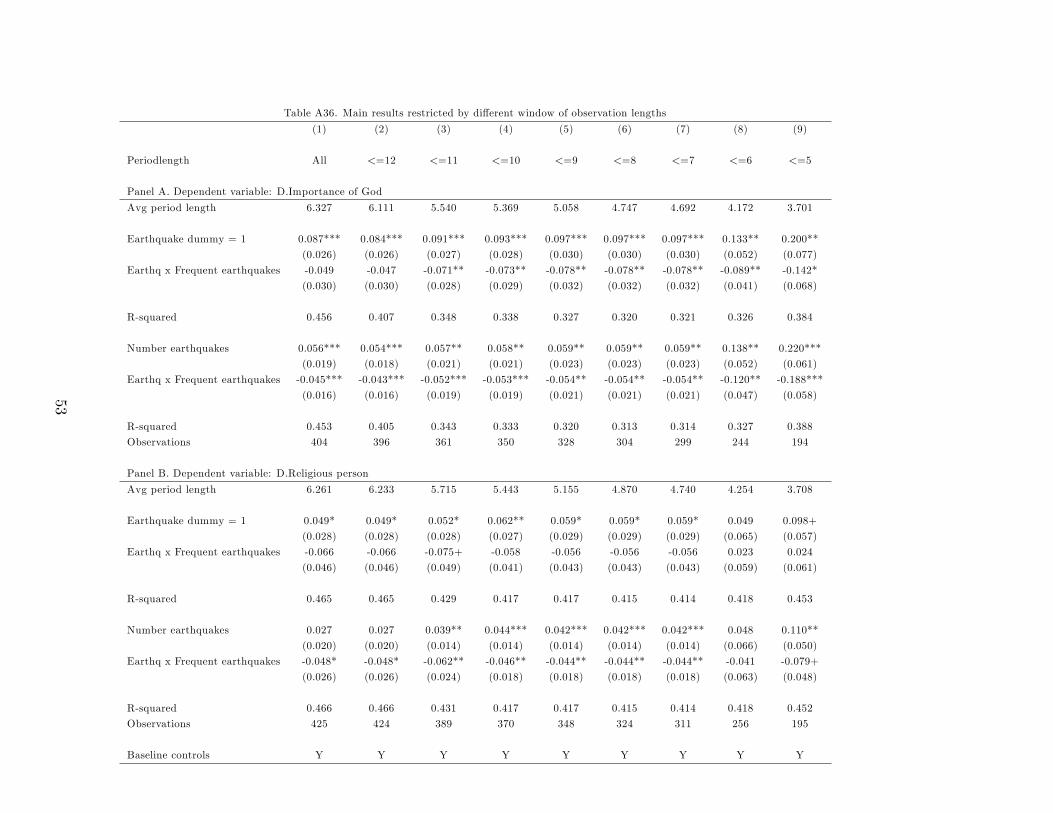
Table A36. Main results restricted by different window of observation lengths

(1) (2) (3) (4) (5) (6) (7) (8) (9)

Periodlength All <=12 <=11 <=10 <=9 <=8 <=7 <=6 <=5

Panel A. Dependent variable: D.Importance of God

Avg period length 6.327 6.111 5.540 5.369 5.058 4.747 4.692 4.172 3.701

Earthquake dummy = 1 0.087*** 0.084*** 0.091*** 0.093*** 0.097*** 0.097*** 0.097*** 0.133** 0.200**

(0.026) (0.026) (0.027) (0.028) (0.030) (0.030) (0.030) (0.052) (0.077)

Earthq x Frequent earthquakes -0.049 -0.047 -0.071** -0.073** -0.078** -0.078** -0.078** -0.089** -0.142*

(0.030) (0.030) (0.028) (0.029) (0.032) (0.032) (0.032) (0.041) (0.068)

R-squared 0.456 0.407 0.348 0.338 0.327 0.320 0.321 0.326 0.384

Number earthquakes 0.056*** 0.054*** 0.057** 0.058** 0.059** 0.059** 0.059** 0.138** 0.220***

(0.019) (0.018) (0.021) (0.021) (0.023) (0.023) (0.023) (0.052) (0.061)

Earthq x Frequent earthquakes -0.045*** -0.043*** -0.052*** -0.053*** -0.054** -0.054** -0.054** -0.120** -0.188***

(0.016) (0.016) (0.019) (0.019) (0.021) (0.021) (0.021) (0.047) (0.058)

R-squared 0.453 0.405 0.343 0.333 0.320 0.313 0.314 0.327 0.388

Observations 404 396 361 350 328 304 299 244 194

Panel B. Dependent variable: D.Religious person

Avg period length 6.261 6.233 5.715 5.443 5.155 4.870 4.740 4.254 3.708

Earthquake dummy = 1 0.049* 0.049* 0.052* 0.062** 0.059* 0.059* 0.059* 0.049 0.098+

(0.028) (0.028) (0.028) (0.027) (0.029) (0.029) (0.029) (0.065) (0.057)

Earthq x Frequent earthquakes -0.066 -0.066 -0.075+ -0.058 -0.056 -0.056 -0.056 0.023 0.024

(0.046) (0.046) (0.049) (0.041) (0.043) (0.043) (0.043) (0.059) (0.061)

R-squared 0.465 0.465 0.429 0.417 0.417 0.415 0.414 0.418 0.453

Number earthquakes 0.027 0.027 0.039** 0.044*** 0.042*** 0.042*** 0.042*** 0.048 0.110**

(0.020) (0.020) (0.014) (0.014) (0.014) (0.014) (0.014) (0.066) (0.050)

Earthq x Frequent earthquakes -0.048* -0.048* -0.062** -0.046** -0.044** -0.044** -0.044** -0.041 -0.079+

(0.026) (0.026) (0.024) (0.018) (0.018) (0.018) (0.018) (0.063) (0.048)

R-squared 0.466 0.466 0.431 0.417 0.417 0.415 0.414 0.418 0.452

Observations 425 424 389 370 348 324 311 256 195

Baseline controls Y Y Y Y Y Y Y Y Y

53

Table A36 cont. Main results restricted by different window of observation lengths

(1) (2) (3) (4) (5) (6) (7) (8) (9)

Periodlength All <=12 <=11 <=10 <=9 <=8 <=7 <=6 <=5

Panel C. Dependent variable: D.Attend religious services

Avg period length 6.349 6.322 5.829 5.573 5.304 4.870 4.740 4.254 3.708

Earthquake dummy 0.024 0.024 0.019 0.024 0.025 0.025 0.025 0.068 -0.051

(0.043) (0.043) (0.045) (0.044) (0.048) (0.048) (0.048) (0.095) (0.041)

Earthq x Frequent earthq -0.010 -0.010 0.004 0.014 0.013 0.013 0.013 -0.058 0.033

(0.065) (0.065) (0.075) (0.077) (0.080) (0.080) (0.080) (0.086) (0.067)

R-squared 0.512 0.512 0.513 0.513 0.502 0.486 0.486 0.488 0.214

Number earthquakes 0.019 0.019 0.015 0.017 0.018 0.018 0.018 0.070 -0.055

(0.021) (0.021) (0.022) (0.022) (0.023) (0.023) (0.024) (0.097) (0.040)

Earthq x Frequent earthq -0.031 -0.031 -0.026 -0.018 -0.018 -0.018 -0.018 -0.065 0.048

(0.022) (0.022) (0.024) (0.025) (0.026) (0.026) (0.026) (0.089) (0.038)

R-squared 0.513 0.513 0.513 0.513 0.501 0.485 0.485 0.488 0.214

Observations 439 438 403 384 362 324 311 256 195

Baseline controls Y Y Y Y Y Y Y Y Y

Notes. OLS estimates. The dependent variables are changes in district average importance of God in Panel A, the share of religious

persons in Panel B, and average attendance at religious services in Panel C. Each panel includes two types of regressions using the

earthquake dummy and the number of earthquakes.

54

Table A37. OLS estimates of period lengths on the main variables

(1) (2) (3) (4) (5) (6) (7) (8) (9) (10) (11) (12)

Earthquake measure: Earthquake dummy Number earthquakes

Dependent variable: Period length

Earthquake measure -0.001 -0.019 0.033 -0.007 0.000 -0.006 0.006 0.012 0.049 0.022 0.027 0.022

(0.018) (0.049) (0.072) (0.056) (0.064) (0.055) (0.010) (0.041) (0.059) (0.043) (0.052) (0.046)

Earthq x Frequent earthquakes 0.106 0.316 0.230 0.233 0.251 0.236 0.021 0.025 -0.015 0.010 0.005 0.009

(0.090) (0.248) (0.198) (0.199) (0.204) (0.184) (0.030) (0.037) (0.048) (0.047) (0.050) (0.045)

Years since an earthquake hit -0.000 -0.002 -0.001 -0.001 -0.001 -0.001 -0.000 -0.001 -0.001 -0.001 -0.001 -0.001

(0.001) (0.002) (0.002) (0.002) (0.002) (0.002) (0.001) (0.002) (0.002) (0.002) (0.002) (0.002)

Average education 0.098 0.095

(0.109) (0.106)

Average income 0.119 0.118

(0.088) (0.086)

Share males 0.297 0.306

(0.455) (0.449)

Average age 0.001 0.001

(0.014) (0.013)

Share married -0.000 -0.005

(0.837) (0.832)

Observations 2,159 717 669 785 775 788 2,159 717 669 785 775 788

R-squared 0.879 0.882 0.856 0.883 0.883 0.883 0.880 0.882 0.857 0.884 0.884 0.884

Notes. OLS estimates. The dependent variable is period length measured by the number of years between interviews. The measure of earthquakes is the earthquake

dummy in columns (1)-(6) and the number of earthquakes in columns (7)-(12).

55

An alternative way to test the dynamics is to estimate the district aggregate of equation

(1) with district fixed effects and adding lags of earthquakes. This is done in Table A38

on the full sample. Past earthquakes are aggregated into groups of three years, since

there is too much noise and too few earthquakes in the year-intervals of 1 or 2 years.

"Earthquakes t-1 - t-3" measures whether earthquakes hit the district within the past

three years, measuring earthquakes by the earthquake dummy in columns (1)-(3) and the

number of earthquakes in columns (4)-(6). "Earthquakes t-4 — t-6" measures whether

earthquakes hit between four and six years ago, "Earthquakes t-7 —t-9" between seven

and nine years ago, and "Earthquakes t10-12" between ten and twelve years ago. All

columns include district fixed effects, country-by-year fixed effects, and the remaining

baseline controls. Panel A estimates the simple linear effect, while Panel B includes the

interaction with the "Frequent earthquakes" dummy.

Earthquakes that hit within the last nine years increase intrinsic religiosity significantly

more than earthquakes that hit longer time ago. The result is again stronger on the

intensive margin; average importance of God is affected more than the share of religious

persons. Again, churchgoing is not affected. There is, however, a negative effect from

earthquakes 10-12 years ago, which seems odd and is neither consistent with religious

coping nor a pure economic effect.

56

Title A38. OLS estimates of religiosity on different lags of earthquakes

(1) (2) (3) (4) (5) (6)

Earthquake measure Earthquake dummy Number earthquakes

Dependent variable impgod rel_pers service impgod rel_pers service

Panel A. Baseline regressions

Earthquakes t-1 - t-3 0.063*** 0.036** -0.035 0.021* 0.012* -0.009

(0.016) (0.016) (0.023) (0.011) (0.007) (0.006)

Earthquakes t-4 - t-6 0.010 -0.018 0.038 0.005 -0.013 0.009

(0.019) (0.023) (0.037) (0.006) (0.010) (0.013)

Earthquakes t-7 - t-9 0.032 0.027 -0.012 0.015 0.015 -0.001

(0.020) (0.023) (0.024) (0.012) (0.014) (0.017)

Earthquakes t-10 - t-12 0.011 0.034* -0.055*** 0.003 0.011 -0.027***

(0.011) (0.020) (0.011) (0.006) (0.011) (0.007)

R-squared 0.950 0.926 0.920 0.949 0.926 0.919

Panel B. Interactions with high earthquake frequency

Earthquakes t-1 - t-3 0.087*** 0.045** -0.041 0.061*** 0.023 -0.020

(0.017) (0.017) (0.025) (0.014) (0.016) (0.017)

x High frequency -0.073*** -0.023 0.038 -0.059*** -0.016 0.007

(0.020) (0.025) (0.031) (0.015) (0.017) (0.015)

Earthquakes t-4 - t-6 0.052** -0.006 0.061 0.034** -0.006 0.049

(0.022) (0.034) (0.047) (0.014) (0.022) (0.032)

x High frequency -0.114*** -0.048 -0.082* -0.048*** -0.019 -0.071**

(0.031) (0.039) (0.041) (0.017) (0.028) (0.033)

Earthquakes t-7 - t-9 0.061** 0.019 -0.026 0.040** 0.008 -0.016

(0.023) (0.026) (0.023) (0.019) (0.017) (0.018)

x High frequency -0.055* 0.036 0.061 -0.031 0.022 0.050**

(0.027) (0.033) (0.044) (0.019) (0.017) (0.021)

Earthquakes t-10 - t-12 0.018 0.027 -0.054*** 0.014 0.018 -0.033***

(0.011) (0.022) (0.013) (0.010) (0.017) (0.012)

x High frequency -0.039** 0.020 -0.034* -0.024** -0.016 -0.005

(0.018) (0.028) (0.020) (0.009) (0.017) (0.013)

R-squared 0.951 0.926 0.921 0.950 0.926 0.921

Observations 687 716 744 687 716 744

District FE Y Y Y Y Y Y

Country-by-year FE Y Y Y Y Y Y

Remaining baseline controls N Y N Y N Y

Notes. OLS estimates. The unit of analysis is a district at time t. The dependent variable is average importance of God in

columns (1)-(2) and (5)-(6) and the share of religious persons in columns (3)-(4) and (7-8). The earthquake measure is the

earthquake dummy in columns (1)-(4) and the number of earthquakes in columns (5)-(8). Panel A estimates the simple

linear effect, while Panel B includes the interaction between the earthquake measure and the dummy variable equal to

one if the district was hit by 7 earthquakes or more over the period 1973-2014. All columns include a constant. Standard

errors (in parenthesis) are clustered at the country level. Asterisks ***, **, *, and + indicate significance at the 1, 5, 10,

and 15% level, respectively.

57

C.8 Sample restricted to districts with earthquakes

Table A39 restricts the sample to districts that had at least one earthquake in between

survey rounds. The table shows that religiosity increased more in districts with more

earthquakes in districts that were otherwise rarely hit, compared to districts that were

frequently hit by earthquakes.

Table A39. Main results restricted to districts with at least one earthquake

(1) (2) (3) (4) (5) (6)

Dep. var. D.impgod D.rel_pers D.service

Number earthquakes 0.023*** 0.019** 0.061*** 0.062*** 0.052** 0.064***

(0.004) (0.007) (0.002) (0.001) (0.018) (0.009)

Earthq x frequent earthq -0.042** -0.033* -0.079*** -0.073*** -0.121* -0.159***

(0.013) (0.014) (0.007) (0.003) (0.049) (0.023)

Observations 26 24 26 24 26 24

R-squared 0.861 0.770 0.543 0.484 0.628 0.761

Baseline controls Y Y Y Y Y Y

Inc and edu dummies N Y N Y N Y

Districts 24 24 24 24 24 24

Countries 6 6 6 6 6 6

C.9 Future earthquakes

To construct future earthquakes in years after the latest measure of the religiosity measure,

I choose five-year period lengths, as this is the most common period length (Section C.7).

Instead of the placebo test in Panel C of Table 4, one could also do a horse race between

future and current earthquakes.63 Panel A of Table A40 confirms that earthquakes in

between survey rounds increase religiosity, while future earthquakes do not. This is despite

the high correlation between current and future earthquakes (ρ =0.47). Panel B allows

the impact of the earthquakes to differ with the frequency with which the district is

otherwise hit. Current earthquakes still increase religiosity. Future earthquakes do not,

except in columns (1) and (2), where future earthquakes reduce religiosity in districts

that are frequently hit. This result should be interpreted with caution, though, as the

correlation between the interaction terms with the frequently hit dummy is 0.85. The

variance inflation factor of the interaction term between frequent and future earthquakes

in col (1) of Panel B is 16.55, and the results potentially suffer from multicollinearity.

63Thanks to an anonymous referee for suggesting this.

58

Table A40. Main results including future earthquakes

(1) (2) (3) (4) (5) (6) (7) (8) (9) (10) (11) (12)

Dep. var.: D.impgod D.relpers D.service D.impgod D.relpers D.service

Earthq measure: Earthquake dummy Number earthquakes

Panel A. Simple horserace

Earthquake t 0.076*** 0.073*** 0.052** 0.048** 0.035 0.031 0.032*** 0.028*** 0.019*** 0.017*** 0.016* 0.015

(0.023) (0.022) (0.021) (0.020) (0.030) (0.038) (0.011) (0.009) (0.005) (0.005) (0.009) (0.009)

Earthquake t+1 -0.012 -0.007 0.040 0.039 -0.009 -0.003 -0.012 -0.012 0.008 0.008 -0.004 -0.002

(0.015) (0.019) (0.024) (0.028) (0.049) (0.048) (0.008) (0.008) (0.010) (0.009) (0.014) (0.015)

Observations 350 324 370 333 384 347 350 324 370 333 384 347

R-squared 0.335 0.314 0.416 0.415 0.509 0.507 0.327 0.306 0.413 0.412 0.508 0.506

Baseline controls Y Y Y Y Y Y Y Y Y Y Y Y

Inc and edu dummies N Y N Y N Y N Y N Y N Y

Districts 236 236 236 236 236 236 236 230 250 240 264 254

Countries 31 30 31 30 32 31 31 30 31 30 32 31

Panel B. Horserace including interaction with frequently hit districts

Earthquake t 0.092*** 0.087*** 0.068** 0.066** 0.012 0.008 0.057** 0.052** 0.045*** 0.045*** 0.013 0.012

(0.030) (0.026) (0.031) (0.028) (0.051) (0.058) (0.022) (0.022) (0.016) (0.015) (0.025) (0.028)

Earthq t x Frequent -0.050+ -0.036 -0.064 -0.070* 0.008 0.041 -0.048** -0.043* -0.046** -0.046*** -0.011 -0.011

(0.033) (0.044) (0.051) (0.040) (0.073) (0.088) (0.022) (0.023) (0.020) (0.016) (0.026) (0.030)

Earthquake t+1 -0.007 -0.000 0.034 0.038 -0.061 -0.055 -0.014 -0.006 0.013 0.018 -0.048 -0.038

(0.027) (0.031) (0.043) (0.049) (0.052) (0.050) (0.021) (0.024) (0.032) (0.035) (0.037) (0.035)

Earthq t+1 x Frequent -0.064** -0.076* -0.023 -0.028 0.093 0.088 0.001 -0.003 -0.014 -0.015 0.034 0.030

(0.029) (0.038) (0.068) (0.067) (0.057) (0.052) (0.023) (0.027) (0.032) (0.036) (0.038) (0.035)

Observations 350 324 370 333 384 347 350 324 370 333 384 347

R-squared 0.340 0.318 0.418 0.416 0.518 0.517 0.334 0.311 0.417 0.416 0.517 0.515

Baseline controls Y Y Y Y Y Y Y Y Y Y Y Y

Inc and edu dummies N Y N Y N Y N Y N Y N Y

Districts 236 236 236 236 236 236 236 230 250 240 264 254

Countries 31 30 31 30 32 31 31 30 31 30 32 31

59

C.10 Different magnitudes

The main results are based on earthquakes of magnitude 6 or above. Table A41 uses

different magnitude cut-offs, ranging from 5 or above in columns (1) and (7) to 6.5 or

above in columns (6) and (12). The magnitude scale is logarithmic, so the shaking felt

at magnitude 6 is ten times larger than the magnitude felt at magnitude 5. The rea-

son for showing both results for earthquakes of magnitudes 5 and above and results for

earthquakes of above 5 in magnitude is that many earthquake cluster around the even

numbers, due to rounding errors.

The impact of earthquakes on intrinsic religiosity increases with most magnitude in-

creases. Further, it takes larger earthquakes to influence the extensive margin (religious

person) compared to the intensive margin (importance of God). Attending religious ser-

vices is not influenced throughout, except when restricting the earthquake measure to

include only earthquakes of magnitudes greater than 6.5. Oddly enough, here earthquakes

reduce attendance rates in low-risk districts, which is neither consistent with religious cop-

ing nor a pure economic effect. This result, though, may be influenced by outliers, as there

are only 16 districts in the sample with earthquakes of magnitudes above 6.5. Excluding

outliers removes the negative effect on religious services (not shown), but in this sample,

the interaction with frequent earthquakes is not estimated, and the two estimations are

not directly comparable.

The reason for the change in the number of observations is that the analysis - in line

with the main analysis - excludes district-years with earthquakes in the same year as the

interview.

60

Table A41. Main results for different earthquake magnitudes

(1) (2) (3) (4) (5) (6) (7) (8) (9) (10) (11) (12)

Earthquake measure: Earthquake dummy Number earthquakes

Panel A. Dependent variable: D. importance of God

Earthquake measure 0.012 0.044 0.052** 0.093*** 0.088*** 0.088*** 0.009 0.018 0.034*** 0.058** 0.054** 0.088***

(0.016) (0.031) (0.020) (0.028) (0.031) (0.029) (0.009) (0.015) (0.012) (0.021) (0.021) (0.029)

Earthquake x Frequent earthq 0.023 -0.073** -0.087** -0.080*** -0.030** -0.053*** -0.052** -0.088***

(0.019) (0.029) (0.038) (0.028) (0.012) (0.019) (0.020) (0.028)

Observations 278 282 318 350 350 365 278 282 318 350 350 365

R-squared 0.297 0.297 0.314 0.338 0.335 0.332 0.300 0.295 0.312 0.333 0.330 0.331

No. districts w earthq 57 48 32 29 26 15 57 48 32 29 26 15

Panel B. Dependent variable: D. religious person

Earthquake measure -0.054 -0.006 -0.010 0.062** 0.070*** 0.066*** -0.001 0.010* -0.014 0.044*** 0.047*** 0.065***

(0.041) (0.024) (0.039) (0.027) (0.023) (0.017) (0.005) (0.006) (0.018) (0.014) (0.013) (0.016)

Earthquake x Frequent earthq -0.009 -0.058 -0.056 -0.003 0.027 -0.046** -0.050** -0.044*

(0.040) (0.041) (0.048) (0.037) (0.018) (0.018) (0.021) (0.026)

Observations 298 302 338 370 370 386 298 302 338 370 370 386

R-squared 0.393 0.379 0.401 0.417 0.418 0.419 0.383 0.380 0.401 0.417 0.417 0.417

No. districts w earthq 61 52 33 29 26 16 61 52 33 29 26 16

Panel C. Dependent variable: D. attend religious services

Earthquake measure -0.015 -0.007 -0.007 0.024 -0.021 -0.045** -0.010 -0.009 -0.015 0.017 0.001 -0.045**

(0.018) (0.017) (0.035) (0.044) (0.027) (0.017) (0.007) (0.011) (0.018) (0.022) (0.015) (0.017)

Earthquake x Frequent earthq 0.145*** 0.014 0.019 0.076*** 0.072*** -0.018 -0.009 0.067***

(0.028) (0.077) (0.038) (0.021) (0.018) (0.025) (0.017) (0.017)

Observations 312 316 352 384 384 400 312 316 352 384 384 400

R-squared 0.515 0.528 0.521 0.513 0.516 0.513 0.518 0.529 0.528 0.513 0.516 0.513

No. districts w earthq 63 54 33 29 26 16 63 54 33 29 26 16

Magnitude >=5 >5 >=5.5 >=6 >6 >=6.5 >=5 >5 >=5.5 >=6 >6 >=6.5

Baseline controls Y Y Y Y Y Y Y Y Y Y Y Y

Notes. OLS estimates. The dependent variable is the change in the district aggregate of importance of God in your life in Panel A, the share of religious

persons in Panel B, and average attendance at religious services in Panel C. Earthquakes are measured using the dummy in columns (1)-(6) and

the number of earthquakes in columns (7)-(12). Only earthquakes above magnitude x are included in the analysis, where x ranges from magnitude 5 in

columns (1) and (7) to magnitude 6.5 in columns (6) and (12). Baseline controls are the same as those in Table 4.

61

C.11 Alternative religiosity measures

The main analysis includes only the three measures of religiosity with the most observa-

tions. Table A42 shows the results for the remaining measures of religiosity. Earthquakes

do not increase believing when measured by the three individual measures; whether or not

a person finds comfort in religion, believes in God, or believes in an Afterlife. Whether

this is evidence of the tendency that conversion rates are harder to influence or whether

this is simply due to the reduced sample size is not possible to say. The two compos-

ite measures Strength of Religiosity Scale and Strength of Intrinsic Religiosity Scale are

significantly affected by earthquakes (columns 7-10).

62

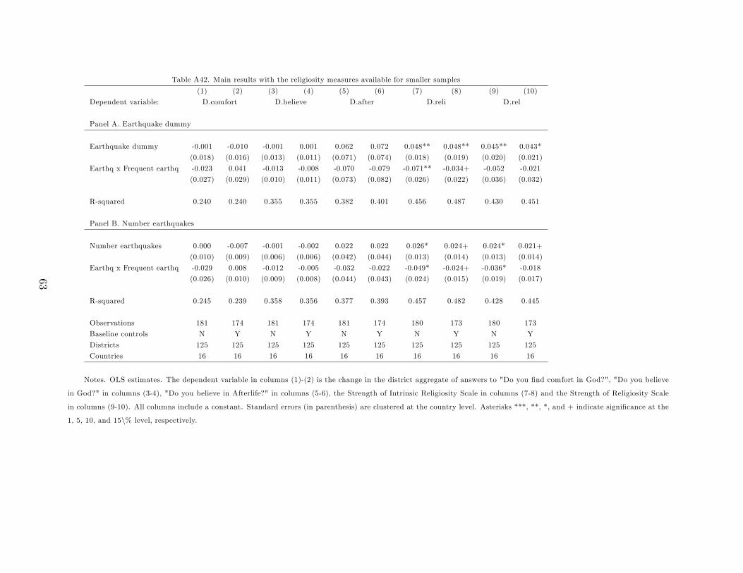
Table A42. Main results with the religiosity measures available for smaller samples

(1) (2) (3) (4) (5) (6) (7) (8) (9) (10)

Dependent variable: D.comfort D.believe D.after D.reli D.rel

Panel A. Earthquake dummy

Earthquake dummy -0.001 -0.010 -0.001 0.001 0.062 0.072 0.048** 0.048** 0.045** 0.043*

(0.018) (0.016) (0.013) (0.011) (0.071) (0.074) (0.018) (0.019) (0.020) (0.021)

Earthq x Frequent earthq -0.023 0.041 -0.013 -0.008 -0.070 -0.079 -0.071** -0.034+ -0.052 -0.021

(0.027) (0.029) (0.010) (0.011) (0.073) (0.082) (0.026) (0.022) (0.036) (0.032)

R-squared 0.240 0.240 0.355 0.355 0.382 0.401 0.456 0.487 0.430 0.451

Panel B. Number earthquakes

Number earthquakes 0.000 -0.007 -0.001 -0.002 0.022 0.022 0.026* 0.024+ 0.024* 0.021+

(0.010) (0.009) (0.006) (0.006) (0.042) (0.044) (0.013) (0.014) (0.013) (0.014)

Earthq x Frequent earthq -0.029 0.008 -0.012 -0.005 -0.032 -0.022 -0.049* -0.024+ -0.036* -0.018

(0.026) (0.010) (0.009) (0.008) (0.044) (0.043) (0.024) (0.015) (0.019) (0.017)

R-squared 0.245 0.239 0.358 0.356 0.377 0.393 0.457 0.482 0.428 0.445

Observations 181 174 181 174 181 174 180 173 180 173

Baseline controls N Y N Y N Y N Y N Y

Districts 125 125 125 125 125 125 125 125 125 125

Countries 16 16 16 16 16 16 16 16 16 16

Notes. OLS estimates. The dependent variable in columns (1)-(2) is the change in the district aggregate of answers to "Do you find comfort in God?", "Do you believe

in God?" in columns (3-4), "Do you believe in Afterlife?" in columns (5-6), the Strength of Intrinsic Religiosity Scale in columns (7-8) and the Strength of Religiosity Scale

in columns (9-10). All columns include a constant. Standard errors (in parenthesis) are clustered at the country level. Asterisks ***, **, *, and + indicate significance at the

1, 5, 10, and 15\% level, respectively.

63

Table A43 shows that insignificance is not due to the smaller sample size.

Table A43. Main results restricted to the sample of the remaining religiosity measures

(1) (2) (3) (4) (5) (6)

Earthquake measure Dummy Number

Dependent variable: D.impgod D.rel_pers D.service D.impgod D.rel_pers D.service

Earthquake dummy 0.092*** 0.097** 0.039 0.052** 0.062** 0.026

(0.031) (0.041) (0.052) (0.021) (0.023) (0.025)

inst_high -0.072* -0.074 0.042 -0.051** -0.057** 0.002

(0.034) (0.051) (0.098) (0.021) (0.023) (0.030)

Observations 173 174 174 173 174 174

R-squared 0.300 0.534 0.353 0.289 0.533 0.350

Baseline controls Y Y Y Y Y Y

C.11.1 Different categorizations of the religiosity measures

This section investigates the results viz-a-viz different categorizations of the two religiosity

measures that are not dummy variables. The different categorizations are described in

Section B.11. Again the importance of God measure is robust to different categorizations

and the impact of earthquake risk is stemming exclusively from the intensive margin.

Attendance at religious services is unaffected by earthquake risk throughout.

Table A44. Main results with different categorizations of the measure of churchgoing

(1) (2) (3) (4) (5) (6)

Dependent variable: Attendance at religious services

Earthquake dummy 0.035 0.034 0.037 0.058 0.001 0.011

(0.029) (0.030) (0.043) (0.053) (0.018) (0.049)

Observations 384 384 384 384 384 383

R-squared 0.500 0.509 0.437 0.350 0.691 0.309

Baseline controls Y Y Y Y Y Y

Attendance measure org base frequent1 frequent2 extensive intensive

64

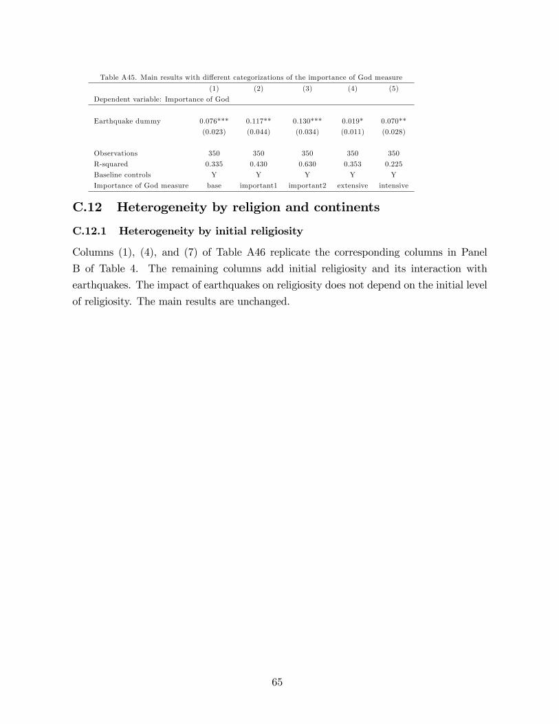
Table A45. Main results with different categorizations of the importance of God measure

(1) (2) (3) (4) (5)

Dependent variable: Importance of God

Earthquake dummy 0.076*** 0.117** 0.130*** 0.019* 0.070**

(0.023) (0.044) (0.034) (0.011) (0.028)

Observations 350 350 350 350 350

R-squared 0.335 0.430 0.630 0.353 0.225

Baseline controls Y Y Y Y Y

Importance of God measure base important1 important2 extensive intensive

C.12 Heterogeneity by religion and continents

C.12.1 Heterogeneity by initial religiosity

Columns (1), (4), and (7) of Table A46 replicate the corresponding columns in Panel

B of Table 4. The remaining columns add initial religiosity and its interaction with

earthquakes. The impact of earthquakes on religiosity does not depend on the initial level

of religiosity. The main results are unchanged.

65

Table A46. Main results including initial religiosity

(1) (2) (3) (4) (5) (6) (7) (8) (9)

Dependent variable: D.impgod D.relpers D.service

Panel A. Earthquake dummy

Earthquake dummy 0.093*** 0.072*** 0.072** 0.062** 0.052*** 0.045** 0.024 0.024 0.005

(0.028) (0.017) (0.030) (0.027) (0.016) (0.020) (0.044) (0.040) (0.024)

Earthq x Frequent earthq -0.073** -0.063*** -0.063*** -0.058 -0.055** -0.048** 0.014 0.032 0.047

(0.029) (0.017) (0.017) (0.041) (0.023) (0.022) (0.077) (0.069) (0.062)

Initital religiosity -0.616*** -0.615*** -0.577*** -0.580*** -0.610*** -0.612***

(0.137) (0.137) (0.091) (0.092) (0.084) (0.084)

Earthq x initial rel -0.008 0.068 0.145

(0.125) (0.065) (0.164)

R-squared 0.338 0.540 0.540 0.417 0.584 0.584 0.513 0.627 0.628

Panel B. Number earthquakes

Number earthquakes 0.058** 0.045*** 0.051*** 0.044*** 0.038*** 0.033*** 0.017 0.021 0.011

(0.021) (0.012) (0.018) (0.014) (0.009) (0.011) (0.022) (0.020) (0.015)

Earthq x Frequent earthq -0.053*** -0.048*** -0.056** -0.046** -0.045*** -0.033** -0.018 -0.017 -0.002

(0.019) (0.012) (0.021) (0.018) (0.012) (0.014) (0.025) (0.023) (0.018)

Initial religiosity -0.620*** -0.617*** -0.578*** -0.579*** -0.609*** -0.609***

(0.138) (0.138) (0.091) (0.091) (0.084) (0.084)

Earthq x initial rel -0.038 0.030 0.080

(0.049) (0.019) (0.051)

R-squared 0.333 0.538 0.538 0.417 0.584 0.584 0.513 0.626 0.628

Observations 350 350 350 370 370 370 384 384 384

Baseline controls Y Y Y Y Y Y Y Y Y

Notes. OLS estimates. The dependent variables are changes in district average of importance of God in columns (1)-(3), the share of religious persons in columns (4)-(6),

and average attendance at religious services in columns (7)-(9). Panel A measures earthquakes with a dummy equal to one if the district was hit by one or more earthquakes.

In Panel B, the earthquake measure is the actual number of earthquakes. Baseline controls are the same as those in Table 4.

66

C.12.2 Heterogeneity by denominations

District-level religiosity is calculated for Christians, Muslims, etc. in Table A47. Like

the corresponding tables in Section B.12, average religiosity is calculated for each denom-

ination separately and thereafter aggregated to the district level. Earthquakes increase

intrinsic religiosity for all denominations, while churchgoing is unaffected across all de-

nominations.

Table A47. Main results restricted to different religious denominations

(1) (2) (3) (4) (5) (6) (7) (8)

Religious denomination All Christian Catholic Protestant Muslim Buddhist Hindu Other

Panel A. Dependent variable: D.importance of God

Earthquake dummy 0.093*** 0.093*** 0.092*** 0.097*** 0.092*** 0.089*** 0.084*** 0.094***

(0.028) (0.027) (0.028) (0.027) (0.028) (0.028) (0.029) (0.027)

Earthq x Frequent earthq -0.073** -0.074** -0.074** -0.075** -0.075** -0.074** -0.069** -0.075**

(0.029) (0.028) (0.028) (0.028) (0.028) (0.028) (0.030) (0.028)

Observations 350 350 350 350 350 350 350 350

R-squared 0.338 0.330 0.326 0.339 0.327 0.323 0.339 0.327

Number earthquakes 0.058** 0.059*** 0.059*** 0.059*** 0.059*** 0.059*** 0.055** 0.059***

(0.021) (0.021) (0.021) (0.021) (0.020) (0.020) (0.021) (0.021)

Earthq x Frequent earthq -0.053*** -0.055*** -0.055*** -0.054*** -0.056*** -0.055*** -0.051** -0.055***

(0.019) (0.019) (0.019) (0.019) (0.018) (0.018) (0.019) (0.019)

Observations 350 350 350 350 350 350 350 350

R-squared 0.333 0.325 0.322 0.332 0.323 0.320 0.336 0.322

Panel B. Dependent variable: D.religious person

Earthquake dummy 0.062** 0.060** 0.059** 0.064** 0.059** 0.065** 0.060** 0.063**

(0.027) (0.027) (0.027) (0.026) (0.026) (0.027) (0.026) (0.028)

Earthq x Frequent earthq -0.058 -0.058 -0.058 -0.060 -0.058 -0.062 -0.058 -0.063

(0.041) (0.041) (0.041) (0.040) (0.041) (0.041) (0.040) (0.042)

Observations 370 370 370 370 370 370 370 370

R-squared 0.417 0.418 0.417 0.420 0.417 0.418 0.421 0.416

Number earthquakes 0.044*** 0.044*** 0.044*** 0.044*** 0.044*** 0.045*** 0.043*** 0.045***

(0.014) (0.013) (0.013) (0.013) (0.013) (0.013) (0.013) (0.014)

Earthq x Frequent earthq -0.046** -0.046** -0.046** -0.046** -0.047** -0.049** -0.046** -0.049**

(0.018) (0.018) (0.018) (0.018) (0.018) (0.018) (0.017) (0.018)

Observations 370 370 370 370 370 370 370 370

R-squared 0.417 0.418 0.417 0.420 0.417 0.417 0.421 0.416

Baseline controls Y Y Y Y Y Y Y Y

67

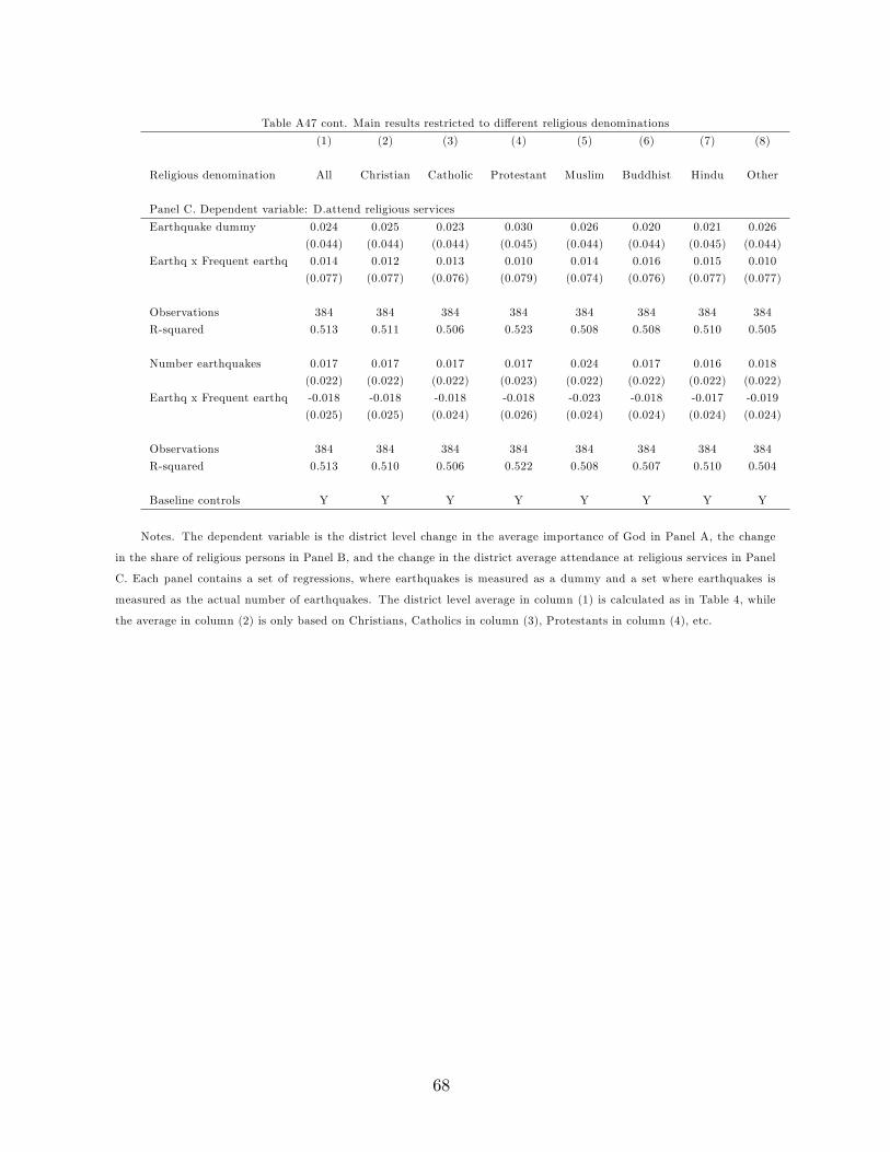
Table A47 cont. Main results restricted to different religious denominations

(1) (2) (3) (4) (5) (6) (7) (8)

Religious denomination All Christian Catholic Protestant Muslim Buddhist Hindu Other

Panel C. Dependent variable: D.attend religious services

Earthquake dummy 0.024 0.025 0.023 0.030 0.026 0.020 0.021 0.026

(0.044) (0.044) (0.044) (0.045) (0.044) (0.044) (0.045) (0.044)

Earthq x Frequent earthq 0.014 0.012 0.013 0.010 0.014 0.016 0.015 0.010

(0.077) (0.077) (0.076) (0.079) (0.074) (0.076) (0.077) (0.077)

Observations 384 384 384 384 384 384 384 384

R-squared 0.513 0.511 0.506 0.523 0.508 0.508 0.510 0.505

Number earthquakes 0.017 0.017 0.017 0.017 0.024 0.017 0.016 0.018

(0.022) (0.022) (0.022) (0.023) (0.022) (0.022) (0.022) (0.022)

Earthq x Frequent earthq -0.018 -0.018 -0.018 -0.018 -0.023 -0.018 -0.017 -0.019

(0.025) (0.025) (0.024) (0.026) (0.024) (0.024) (0.024) (0.024)

Observations 384 384 384 384 384 384 384 384

R-squared 0.513 0.510 0.506 0.522 0.508 0.507 0.510 0.504

Baseline controls Y Y Y Y Y Y Y Y

Notes. The dependent variable is the district level change in the average importance of God in Panel A, the change

in the share of religious persons in Panel B, and the change in the district average attendance at religious services in Panel

C. Each panel contains a set of regressions, where earthquakes is measured as a dummy and a set where earthquakes is

measured as the actual number of earthquakes. The district level average in column (1) is calculated as in Table 4, while

the average in column (2) is only based on Christians, Catholics in column (3), Protestants in column (4), etc.

68

Table A48. Main results including denomination fixed effects

(1) (2) (3) (4) (5) (6)

Dep. var.: D.impgod D.relpers D.service

Panel A. Earthquake measure based on earthquake dummy

Earthquake dummy 0.098*** 0.096*** 0.065** 0.064** 0.008 0.005

(0.030) (0.029) (0.026) (0.027) (0.047) (0.047)

Earthq x Frequent -0.092** -0.081** -0.066* -0.050 -0.014 0.001

(0.038) (0.034) (0.034) (0.036) (0.075) (0.077)

R-squared 0.343 0.315 0.399 0.397 0.281 0.268

Panel A. Earthquake measure based on number of earthquakes

Number earthquakes 0.060** 0.058** 0.047*** 0.046*** 0.008 0.006

(0.023) (0.022) (0.013) (0.014) (0.025) (0.025)

Earthq x Frequent -0.061*** -0.058*** -0.050*** -0.046*** -0.025 -0.022

(0.021) (0.021) (0.015) (0.016) (0.023) (0.023)

R-squared 0.338 0.310 0.399 0.397 0.282 0.269

Observations 338 338 367 367 381 381

Baseline controls Y Y Y Y Y Y

59 denominations FE Y N Y N Y N

6 major denominations FE N Y N Y N Y

Districts 227 227 227 227 227 227

Countries 30 30 31 31 32 32

C.12.3 Heterogeneity by continents

As continents are measured at the district-level, this part of the analysis is done like the

cross-districts analysis. Corroborating the finding of the cross-districts analysis, earth-

quakes increase religiosity across all continents. While there were no differences between

continents in the cross-districts study, Table A49 shows that earthquakes in Europe in-

crease religiosity more than other places, but mainly on the intensive margin (importance

of God and churchgoing). Earthquakes in Oceania only seem to have an impact on

the share of religious persons. The latter only covers 9 districts, though. Churchgoing

is unaffected across all continents, except Europe, where earthquakes tend to increase

churchgoing. The latter is consistent with both religious coping and a pure economic

effect.

69

Table A49. Main results interacted with different continents

(1) (2) (3) (4) (5) (6) (7) (8) (9) (10) (11) (12)

Earthquake measure: Earthquake dummy Number earthquakes

Panel A. Dependent variable: D.Importance of God

Earthquake measure 0.093*** 0.095*** 0.095*** 0.068** 0.098*** 0.089*** 0.058** 0.058** 0.058** 0.052*** 0.060** 0.055**

(0.028) (0.030) (0.028) (0.025) (0.030) (0.028) (0.021) (0.022) (0.022) (0.018) (0.023) (0.020)

Earthq x Frequent earthq -0.073** -0.075** -0.059** -0.067*** -0.079** -0.069** -0.053*** -0.054** -0.053*** -0.053*** -0.054** -0.051***

(0.029) (0.032) (0.022) (0.024) (0.032) (0.029) (0.019) (0.020) (0.018) (0.018) (0.020) (0.018)

Earthquake x Africa -0.032 -0.001

(0.038) (0.032)

Earthquake x America -0.037 -0.005

(0.025) (0.009)

Earthquake x Asia 0.033 0.007

(0.038) (0.017)

Earthquake x Oceania -0.075** -0.063**

(0.035) (0.027)

Earthquake x Europe 0.086*** 0.119***

(0.029) (0.022)

Observations 350 350 350 350 350 350 350 350 350 350 350 350

R-squared 0.338 0.338 0.338 0.339 0.339 0.339 0.333 0.333 0.333 0.333 0.334 0.334

Panel B. Dependent variable: D.Religious person

Earthquake measure 0.062** 0.062** 0.059** 0.106*** 0.058* 0.061** 0.044*** 0.044*** 0.043*** 0.067*** 0.043*** 0.043***

(0.027) (0.027) (0.028) (0.033) (0.029) (0.028) (0.014) (0.014) (0.014) (0.021) (0.014) (0.014)

Earthq x Frequent earthq -0.058 -0.058 -0.080** -0.069* -0.055 -0.058 -0.046** -0.046** -0.050** -0.048** -0.046** -0.045**

(0.041) (0.041) (0.037) (0.034) (0.043) (0.042) (0.018) (0.018) (0.019) (0.019) (0.018) (0.018)

Earthquake x America 0.066 0.029

(0.055) (0.019)

Earthquake x Asia -0.054 -0.026

(0.040) (0.017)

Earthquake x Oceania 0.040 0.003

(0.036) (0.049)

Earthquake x Europe 0.013 0.031*

(0.028) (0.015)

Observations 370 370 370 370 370 370 370 370 370 370 370 370

R-squared 0.417 0.417 0.418 0.418 0.417 0.417 0.417 0.417 0.418 0.418 0.417 0.417

Baseline controls Y Y Y Y Y Y Y Y Y Y Y Y

70

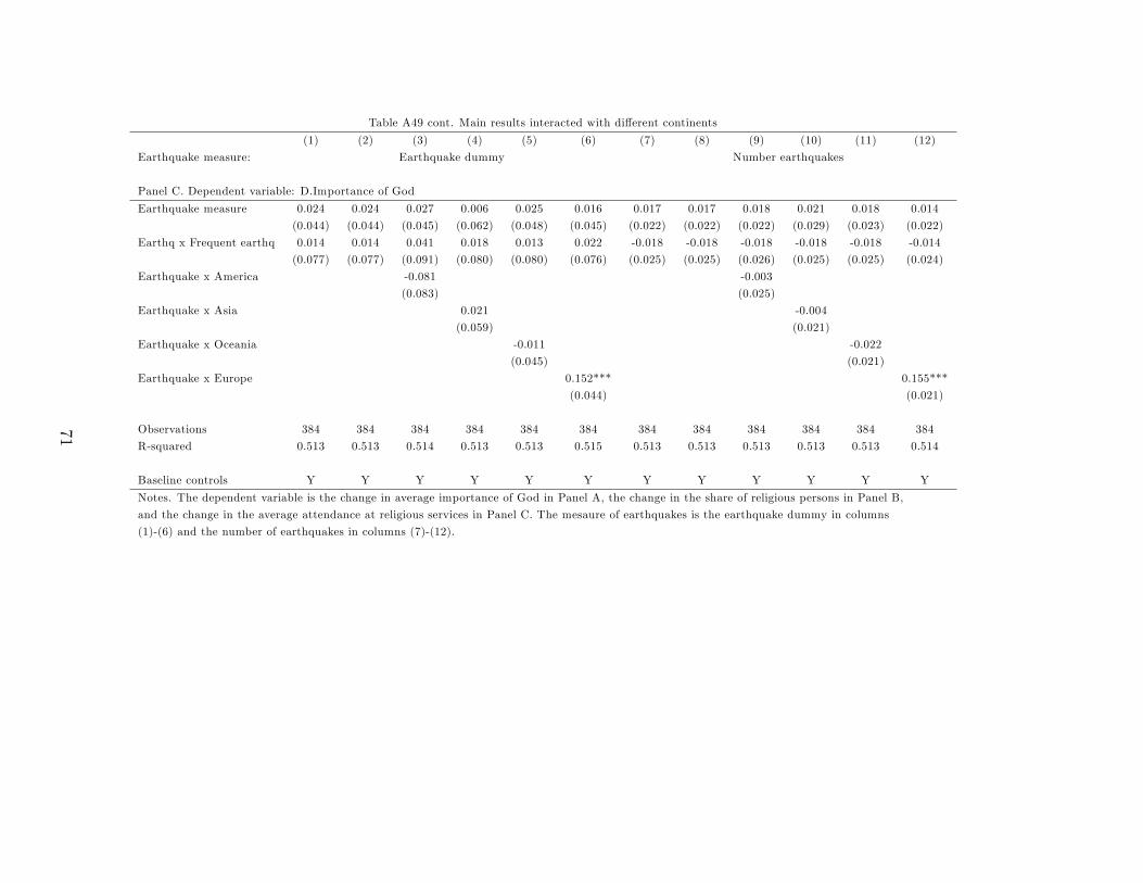
Table A49 cont. Main results interacted with different continents

(1) (2) (3) (4) (5) (6) (7) (8) (9) (10) (11) (12)

Earthquake measure: Earthquake dummy Number earthquakes

Panel C. Dependent variable: D.Importance of God

Earthquake measure 0.024 0.024 0.027 0.006 0.025 0.016 0.017 0.017 0.018 0.021 0.018 0.014

(0.044) (0.044) (0.045) (0.062) (0.048) (0.045) (0.022) (0.022) (0.022) (0.029) (0.023) (0.022)

Earthq x Frequent earthq 0.014 0.014 0.041 0.018 0.013 0.022 -0.018 -0.018 -0.018 -0.018 -0.018 -0.014

(0.077) (0.077) (0.091) (0.080) (0.080) (0.076) (0.025) (0.025) (0.026) (0.025) (0.025) (0.024)

Earthquake x America -0.081 -0.003

(0.083) (0.025)

Earthquake x Asia 0.021 -0.004

(0.059) (0.021)

Earthquake x Oceania -0.011 -0.022

(0.045) (0.021)

Earthquake x Europe 0.152*** 0.155***

(0.044) (0.021)

Observations 384 384 384 384 384 384 384 384 384 384 384 384

R-squared 0.513 0.513 0.514 0.513 0.513 0.515 0.513 0.513 0.513 0.513 0.513 0.514

Baseline controls Y Y Y Y Y Y Y Y Y Y Y Y

Notes. The dependent variable is the change in average importance of God in Panel A, the change in the share of religious persons in Panel B,

and the change in the average attendance at religious services in Panel C. The mesaure of earthquakes is the earthquake dummy in columns

(1)-(6) and the number of earthquakes in columns (7)-(12).

71

C.13 Heterogeneity by development

As the variables in the event study are aggregated to the district level, the interactions

with individual characteristics, such as income levels, is done in a slightly different manner

than in the cross-district study. The complication arises as individual-level controls are

added at the individual level throughout, and thereafter residuals are aggregated.

The baseline result is reproduced in column (1) of Table A49 on the full sample of

individuals of any income deciles. In column (2), average religiosity is calculated only

among individuals with incomes in the lowest decile. Column (3) restricts the sample

to individuals with income among the second decile, and so on until average religiosity

is calculated in column (11) for individuals with the highest incomes only. Earthquakes

influence religiosity similarly across all income deciles with no tendency for higher or

lower incomes groups to respond more or less to earthquakes. Earthquakes do not affect

churchgoing regardless of which income decile, the individual belongs to. The same results

hold for all education groups and unemployed or not (Tables A50 and A51).

The same question is investigated in a slightly different manner in Table A52 with

a focus on district level development. Religiosity is calculated based on the full sample

of individuals and earthquakes are instead interacted with district level income, light

intensity, education, and unemployment rates. The impact of earthquakes on intrinsic

religiosity is larger in districts with lower levels of average income or education, but the

impact does not differ with light intensity or unemployment levels. Churchgoing is again

unaffected by earthquakes, and this is the case across income or education groups, except

that churchgoing does seem to be slightly more affected for those living in districts with

higher average unemployment rates. This latter finding is both consistent with religious

coping and a pure economic effect.

72

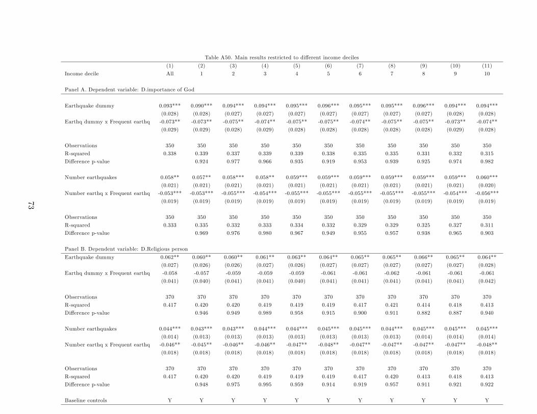
Table A50. Main results restricted to different income deciles

(1) (2) (3) (4) (5) (6) (7) (8) (9) (10) (11)

Income decile All 1 2 3 4 5 6 7 8 9 10

Panel A. Dependent variable: D.importance of God

Earthquake dummy 0.093*** 0.090*** 0.094*** 0.094*** 0.095*** 0.096*** 0.095*** 0.095*** 0.096*** 0.094*** 0.094***

(0.028) (0.028) (0.027) (0.027) (0.027) (0.027) (0.027) (0.027) (0.027) (0.028) (0.028)

Earthq dummy x Frequent earthq -0.073** -0.073** -0.075** -0.074** -0.075** -0.075** -0.074** -0.075** -0.075** -0.073** -0.074**

(0.029) (0.029) (0.028) (0.029) (0.028) (0.028) (0.028) (0.028) (0.028) (0.029) (0.028)

Observations 350 350 350 350 350 350 350 350 350 350 350

R-squared 0.338 0.339 0.337 0.339 0.339 0.338 0.335 0.335 0.331 0.332 0.315

Difference p-value 0.924 0.977 0.966 0.935 0.919 0.953 0.939 0.925 0.974 0.982

Number earthquakes 0.058** 0.057** 0.058*** 0.058** 0.059*** 0.059*** 0.059*** 0.059*** 0.059*** 0.059*** 0.060***

(0.021) (0.021) (0.021) (0.021) (0.021) (0.021) (0.021) (0.021) (0.021) (0.021) (0.020)

Number earthq x Frequent earthq -0.053*** -0.053*** -0.055*** -0.054*** -0.055*** -0.055*** -0.055*** -0.055*** -0.055*** -0.054*** -0.056***

(0.019) (0.019) (0.019) (0.019) (0.019) (0.019) (0.019) (0.019) (0.019) (0.019) (0.019)

Observations 350 350 350 350 350 350 350 350 350 350 350

R-squared 0.333 0.335 0.332 0.333 0.334 0.332 0.329 0.329 0.325 0.327 0.311

Difference p-value 0.969 0.976 0.980 0.967 0.949 0.955 0.957 0.938 0.965 0.903

Panel B. Dependent variable: D.Religious person

Earthquake dummy 0.062** 0.060** 0.060** 0.061** 0.063** 0.064** 0.065** 0.065** 0.066** 0.065** 0.064**

(0.027) (0.026) (0.026) (0.027) (0.026) (0.027) (0.027) (0.027) (0.027) (0.027) (0.028)

Earthq dummy x Frequent earthq -0.058 -0.057 -0.059 -0.059 -0.059 -0.061 -0.061 -0.062 -0.061 -0.061 -0.061

(0.041) (0.040) (0.041) (0.041) (0.040) (0.041) (0.041) (0.041) (0.041) (0.041) (0.042)

Observations 370 370 370 370 370 370 370 370 370 370 370

R-squared 0.417 0.420 0.420 0.419 0.419 0.419 0.417 0.421 0.414 0.418 0.413

Difference p-value 0.946 0.949 0.989 0.958 0.915 0.900 0.911 0.882 0.887 0.940

Number earthquakes 0.044*** 0.043*** 0.043*** 0.044*** 0.044*** 0.045*** 0.045*** 0.044*** 0.045*** 0.045*** 0.045***

(0.014) (0.013) (0.013) (0.013) (0.013) (0.013) (0.013) (0.013) (0.014) (0.014) (0.014)

Number earthq x Frequent earthq -0.046** -0.045** -0.046** -0.046** -0.047** -0.048** -0.047** -0.047** -0.047** -0.047** -0.048**

(0.018) (0.018) (0.018) (0.018) (0.018) (0.018) (0.018) (0.018) (0.018) (0.018) (0.018)

Observations 370 370 370 370 370 370 370 370 370 370 370

R-squared 0.417 0.420 0.420 0.419 0.419 0.419 0.417 0.420 0.413 0.418 0.413

Difference p-value 0.948 0.975 0.995 0.959 0.914 0.919 0.957 0.911 0.921 0.922

Baseline controls Y Y Y Y Y Y Y Y Y Y Y

73

Table A50 cont. Main results restricted to different income deciles

(1) (2) (3) (4) (5) (6) (7) (8) (9) (10) (11)

Income decile All 1 2 3 4 5 6 7 8 9 10

Panel C. Dependent variable: D.attend religious services

Earthquake dummy 0.024 0.021 0.023 0.024 0.024 0.027 0.026 0.025 0.026 0.025 0.024

(0.044) (0.045) (0.045) (0.045) (0.045) (0.044) (0.044) (0.044) (0.043) (0.044) (0.043)

Earthq x Frequent earthq 0.014 0.016 0.014 0.014 0.014 0.012 0.012 0.012 0.012 0.014 0.013

(0.077) (0.077) (0.077) (0.077) (0.077) (0.076) (0.076) (0.076) (0.075) (0.076) (0.075)

Observations 384 384 384 384 384 384 384 384 384 384 384

R-squared 0.513 0.518 0.516 0.516 0.514 0.512 0.509 0.508 0.502 0.506 0.503

Difference p-value 0.960 0.992 0.996 0.995 0.947 0.952 0.978 0.960 0.983 0.993

Number earthquakes 0.017 0.017 0.018 0.018 0.018 0.019 0.019 0.018 0.019 0.018 0.018

(0.022) (0.023) (0.023) (0.023) (0.022) (0.022) (0.022) (0.022) (0.022) (0.022) (0.022)

Earthq x Frequent earthq -0.018 -0.017 -0.018 -0.018 -0.018 -0.020 -0.020 -0.019 -0.020 -0.018 -0.019

(0.025) (0.025) (0.025) (0.025) (0.025) (0.025) (0.024) (0.024) (0.024) (0.024) (0.024)

Observations 384 384 384 384 384 384 384 384 384 384 384

R-squared 0.513 0.517 0.515 0.516 0.514 0.512 0.508 0.507 0.502 0.506 0.502

Difference p-value 0.979 0.993 0.987 0.978 0.934 0.935 0.972 0.947 0.980 0.971

Baseline controls Y Y Y Y Y Y Y Y Y Y Y

Notes. The table replicates Panel B of Table 4, where religiosity is instead measured only across individuals from the particular

income decile. "Difference p-value" indicates the p-value of the test that the estimate on the earthquake measure equals the

estimate in column (1).

74

Table A51. Main results restricted to different education categories

(1) (2) (3) (4) (5) (6) (7) (8) (9)

Education category All 1 2 3 4 5 6 7 8

Panel A. Dependent variable: D.importance of God

Earthquake dummy 0.093*** 0.093*** 0.095*** 0.093*** 0.095*** 0.095*** 0.094*** 0.098*** 0.095***

(0.028) (0.027) (0.027) (0.028) (0.028) (0.027) (0.027) (0.027) (0.027)

Earthq x Frequent earthq -0.073** -0.075** -0.075** -0.072** -0.073** -0.074** -0.074** -0.075** -0.075**

(0.029) (0.028) (0.028) (0.029) (0.029) (0.029) (0.029) (0.029) (0.029)

Observations 350 350 350 350 350 350 350 350 350

R-squared 0.338 0.335 0.338 0.349 0.338 0.351 0.342 0.353 0.346

Difference p-value 0.988 0.927 0.995 0.956 0.933 0.970 0.850 0.948

Number earthquakes 0.058** 0.059*** 0.059*** 0.056** 0.058** 0.057** 0.058** 0.058** 0.058**

(0.021) (0.021) (0.021) (0.022) (0.022) (0.022) (0.021) (0.022) (0.022)

Earthq x Frequent earthq -0.053*** -0.055*** -0.055*** -0.052** -0.054*** -0.053** -0.054*** -0.054** -0.054***

(0.019) (0.019) (0.019) (0.020) (0.019) (0.020) (0.019) (0.020) (0.019)

Observations 350 350 350 350 350 350 350 350 350

R-squared 0.333 0.330 0.332 0.343 0.333 0.344 0.336 0.346 0.340

Difference p-value 0.959 0.966 0.952 0.984 0.979 0.993 0.983 0.991

Panel B. Dependent variable: D.Religious person

Earthquake dummy 0.062** 0.063** 0.061** 0.059** 0.062** 0.062** 0.064** 0.063** 0.064**

(0.027) (0.026) (0.027) (0.026) (0.027) (0.026) (0.026) (0.026) (0.026)

Earthq x Frequent earthq -0.058 -0.060 -0.059 -0.054 -0.059 -0.057 -0.061 -0.058 -0.060

(0.041) (0.040) (0.041) (0.040) (0.041) (0.040) (0.040) (0.040) (0.039)

Observations 370 370 370 370 370 370 370 370 370

R-squared 0.417 0.420 0.418 0.416 0.417 0.420 0.421 0.420 0.423

Difference p-value 0.969 0.976 0.933 0.989 0.997 0.935 0.952 0.916

Number earthquakes 0.044*** 0.045*** 0.044*** 0.042*** 0.044*** 0.043*** 0.044*** 0.043*** 0.044***

(0.014) (0.013) (0.014) (0.014) (0.014) (0.014) (0.013) (0.014) (0.013)

Earthq x Frequent earthq -0.046** -0.047** -0.046** -0.043** -0.046** -0.044** -0.047** -0.045** -0.046**

(0.018) (0.017) (0.018) (0.018) (0.018) (0.018) (0.018) (0.018) (0.017)

Observations 370 370 370 370 370 370 370 370 370

R-squared 0.417 0.420 0.418 0.416 0.417 0.420 0.421 0.420 0.423

Difference p-value 0.940 0.996 0.917 0.989 0.955 0.960 0.980 0.989

Baseline controls Y Y Y Y Y Y Y Y Y

75

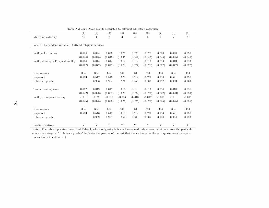
Table A51 cont. Main results restricted to different education categories

(1) (2) (3) (4) (5) (6) (7) (8) (9)

Education category All 1 2 3 4 5 6 7 8

Panel C. Dependent variable: D.attend religious services

Earthquake dummy 0.024 0.024 0.023 0.025 0.026 0.026 0.024 0.028 0.026

(0.044) (0.045) (0.045) (0.045) (0.044) (0.045) (0.045) (0.045) (0.045)

Earthq dummy x Frequent earthq 0.014 0.014 0.014 0.014 0.012 0.013 0.013 0.013 0.013

(0.077) (0.077) (0.077) (0.078) (0.077) (0.078) (0.077) (0.077) (0.077)

Observations 384 384 384 384 384 384 384 384 384

R-squared 0.513 0.517 0.513 0.520 0.512 0.521 0.514 0.521 0.520

Difference p-value 0.996 0.984 0.971 0.956 0.962 0.992 0.933 0.963

Number earthquakes 0.017 0.019 0.017 0.016 0.018 0.017 0.018 0.018 0.018

(0.022) (0.023) (0.022) (0.023) (0.022) (0.023) (0.022) (0.023) (0.023)

Earthq x Frequent earthq -0.018 -0.020 -0.018 -0.016 -0.018 -0.017 -0.018 -0.018 -0.018

(0.025) (0.025) (0.025) (0.025) (0.025) (0.025) (0.025) (0.025) (0.025)

Observations 384 384 384 384 384 384 384 384 384

R-squared 0.513 0.516 0.512 0.519 0.512 0.521 0.514 0.521 0.520

Difference p-value 0.939 0.997 0.952 0.983 0.967 0.989 0.994 0.973

Baseline controls Y Y Y Y Y Y Y Y Y

Notes. The table replicates Panel B of Table 4, where religiosity is instead measured only across individuals from the particular

education category. "Difference p-value" indicates the p-value of the test that the estimate on the earthquake measure equals

the estimate in column (1).

76

Table A52. Main results restricted to different employment status

(1) (2) (3) (4) (5) (6) (7) (8) (9) (10)

Earthquake measure Earthquake dummy Number earthquakes

Sample All Unemployed Employed All Unemployed Employed

Panel A. Dependent variable: D.importance of God

Earthquake measure 0.093*** 0.094*** 0.088*** 0.092*** 0.083*** 0.058** 0.059*** 0.056*** 0.057** 0.053***

(0.028) (0.028) (0.028) (0.028) (0.026) (0.021) (0.021) (0.018) (0.021) (0.018)

Earthq x Frequent earthq -0.073** -0.073** -0.070** -0.073** -0.073** -0.053*** -0.055*** -0.054*** -0.053*** -0.052***

(0.029) (0.029) (0.028) (0.029) (0.027) (0.019) (0.019) (0.017) (0.019) (0.017)

Observations 350 350 276 350 276 350 350 276 350 276

R-squared 0.338 0.335 0.293 0.338 0.284 0.333 0.330 0.290 0.333 0.281

Difference p-value 0.979 0.848 0.976 0.720 0.952 0.930 0.988 0.780

Panel B. Dependent variable: D.religious person

Earthquake measure 0.062** 0.061** 0.058** 0.061** 0.054* 0.044*** 0.043*** 0.040*** 0.043*** 0.039***

(0.027) (0.026) (0.026) (0.027) (0.027) (0.014) (0.014) (0.013) (0.014) (0.013)

Earthq x Frequent earthq -0.058 -0.056 -0.074* -0.058 -0.078* -0.046** -0.044** -0.047** -0.046** -0.048**

(0.041) (0.040) (0.037) (0.041) (0.039) (0.018) (0.017) (0.017) (0.018) (0.018)

Observations 370 370 296 370 296 370 370 296 370 296

R-squared 0.417 0.420 0.391 0.417 0.388 0.417 0.420 0.391 0.417 0.388

Difference p-value 0.984 0.895 0.981 0.767 0.947 0.796 0.993 0.738

Panel C. Dependent variable: D.attend religious services

Earthquake measure 0.024 0.024 0.017 0.023 0.009 0.017 0.018 0.015 0.017 0.011

(0.044) (0.044) (0.044) (0.045) (0.045) (0.022) (0.022) (0.021) (0.022) (0.022)

Earthq x Frequent earthq 0.014 0.015 0.028 0.014 0.022 -0.018 -0.017 -0.013 -0.018 -0.013

(0.077) (0.076) (0.072) (0.077) (0.070) (0.025) (0.024) (0.023) (0.025) (0.022)

Observations 384 384 310 384 310 384 384 310 384 310

R-squared 0.513 0.510 0.483 0.513 0.442 0.513 0.510 0.482 0.512 0.441

Difference p-value 0.993 0.884 0.989 0.755 0.990 0.917 0.997 0.777

Baseline controls Y Y Y Y Y Y Y Y Y Y

Income FE N N Y N Y N N Y N Y

Notes. The table replicates Panel B of Table 4, where religiosity is instead measured only across either employed or unemployed individuals.

Difference p-value indicates the p-value of the test that the estimate equals the estimate in columns (1) and (6).

77

Table A53. Main results interacted with district development

(1) (2) (3) (4) (5) (6) (7)

Panel A. Dependent variable: D.Importance of God

Earthquake dummy 0.510*** 0.099*** 0.251*** 0.108** 0.069*** 0.102*** 0.099***

(0.104) (0.031) (0.090) (0.045) (0.012) (0.031) (0.030)

Earthq x Frequent earthq -0.037 -0.084** -0.085*** -0.078** -0.061*** -0.083** -0.074**

(0.027) (0.036) (0.030) (0.031) (0.022) (0.032) (0.032)

Earthq x development -0.094*** -0.002 -0.037** -0.102 0.307 -0.032 -0.014*

(0.023) (0.002) (0.016) (0.139) (0.402) (0.023) (0.008)

Observations 276 350 348 348 276 350 350

R-squared 0.373 0.339 0.347 0.340 0.357 0.339 0.339

Panel B. Dependent variable: D.Religious person

Earthquake dummy 0.322** 0.068** 0.308*** 0.065 0.070*** 0.090*** 0.061**

(0.132) (0.028) (0.095) (0.048) (0.025) (0.024) (0.029)

Earthq x Frequent earthq -0.039 -0.069 -0.090* -0.061 -0.051 -0.088** -0.065*

(0.050) (0.043) (0.053) (0.044) (0.039) (0.037) (0.038)

Earthq x development -0.059** -0.002 -0.056*** -0.020 -0.154* -0.095*** 0.010

(0.027) (0.002) (0.017) (0.170) (0.077) (0.020) (0.016)

Observations 296 370 368 368 296 370 370

R-squared 0.444 0.418 0.426 0.418 0.437 0.419 0.417

Panel C. Dependent variable: D.Attend religious services

Earthquake dummy 0.204 0.012 0.208 0.036 0.031 -0.017 0.034

(0.326) (0.053) (0.179) (0.064) (0.042) (0.027) (0.047)

Earthq x Frequent earthq 0.030 0.032 0.013 0.009 0.021 0.059 0.025

(0.078) (0.091) (0.081) (0.077) (0.085) (0.052) (0.079)

Earthq x development -0.042 0.005 -0.045 -0.079 -0.145 0.137** -0.040

(0.068) (0.005) (0.032) (0.175) (0.143) (0.063) (0.024)

Observations 310 384 382 382 310 384 384

R-squared 0.529 0.516 0.521 0.514 0.541 0.518 0.515

Development Inc Light Edu Unempl Agri Pdens Area

Baseline controls Y Y Y Y Y Y Y

78

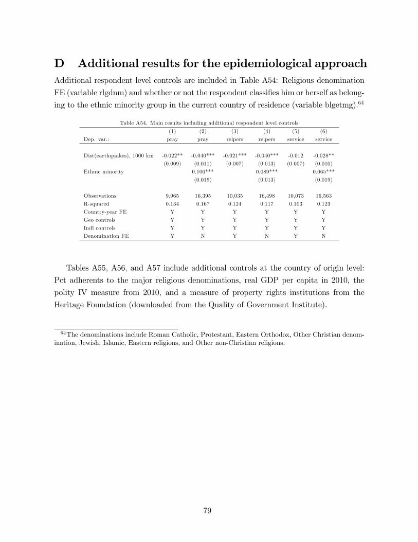
D Additional results for the epidemiological approachAdditional respondent level controls are included in Table A54: Religious denomination

FE (variable rlgdnm) and whether or not the respondent classifies him or herself as belong-

ing to the ethnic minority group in the current country of residence (variable blgetmg).64

Table A54. Main results including additional respondent level controls

(1) (2) (3) (4) (5) (6)

Dep. var.: pray pray relpers relpers service service

Dist(earthquakes), 1000 km -0.022** -0.040*** -0.021*** -0.040*** -0.012 -0.028**

(0.009) (0.011) (0.007) (0.013) (0.007) (0.010)

Ethnic minority 0.106*** 0.089*** 0.065***

(0.019) (0.013) (0.019)

Observations 9,965 16,395 10,035 16,498 10,073 16,563

R-squared 0.134 0.167 0.124 0.117 0.103 0.123

Country-year FE Y Y Y Y Y Y

Geo controls Y Y Y Y Y Y

Indl controls Y Y Y Y Y Y

Denomination FE Y N Y N Y N

Tables A55, A56, and A57 include additional controls at the country of origin level:

Pct adherents to the major religious denominations, real GDP per capita in 2010, the

polity IV measure from 2010, and a measure of property rights institutions from the

Heritage Foundation (downloaded from the Quality of Government Institute).

64The denominations include Roman Catholic, Protestant, Eastern Orthodox, Other Christian denom-ination, Jewish, Islamic, Eastern religions, and Other non-Christian religions.

79

Table A55. Main results with additional country of origin controls

(1) (2) (3) (4) (5) (6) (7) (8)

Dep. var.: Prayer outside religious services

Dist(earthquakes), 1000 km -0.032** -0.041*** -0.043*** -0.041*** -0.043*** -0.043*** -0.043*** -0.040***

(0.013) (0.013) (0.013) (0.013) (0.013) (0.013) (0.013) (0.013)

Percent Muslims 0.094***

(0.034)

Percent Christians -0.025

(0.036)

Percent Jews -0.008

(0.051)

Percent Buddhists -0.152*

(0.080)

Percent Hindus -0.024

(0.038)

Real GDP per capita 2010 0.001

(0.005)

Polity IV 2010 -0.002

(0.001)

Property Rights -0.000

(0.000)

Observations 16,499 16,499 16,499 16,499 16,499 16,499 16,565 16,937

R-squared 0.163 0.162 0.162 0.162 0.162 0.162 0.159 0.159

Country-year FE Y Y Y Y Y Y Y Y

Geo controls Y Y Y Y Y Y Y Y

Indl controls Y Y Y Y Y Y Y Y

80

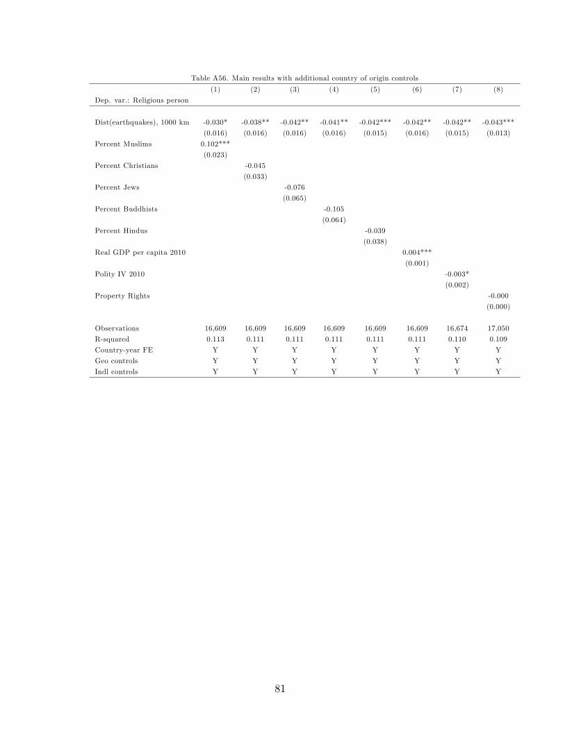
Table A56. Main results with additional country of origin controls

(1) (2) (3) (4) (5) (6) (7) (8)

Dep. var.: Religious person

Dist(earthquakes), 1000 km -0.030* -0.038** -0.042** -0.041** -0.042*** -0.042** -0.042** -0.043***

(0.016) (0.016) (0.016) (0.016) (0.015) (0.016) (0.015) (0.013)

Percent Muslims 0.102***

(0.023)

Percent Christians -0.045

(0.033)

Percent Jews -0.076

(0.065)

Percent Buddhists -0.105

(0.064)

Percent Hindus -0.039

(0.038)

Real GDP per capita 2010 0.004***

(0.001)

Polity IV 2010 -0.003*

(0.002)

Property Rights -0.000

(0.000)

Observations 16,609 16,609 16,609 16,609 16,609 16,609 16,674 17,050

R-squared 0.113 0.111 0.111 0.111 0.111 0.111 0.110 0.109

Country-year FE Y Y Y Y Y Y Y Y

Geo controls Y Y Y Y Y Y Y Y

Indl controls Y Y Y Y Y Y Y Y

81

Table A57. Main results with additional country of origin controls

(1) (2) (3) (4) (5) (6) (7) (8)

Dep. var.: Attendance at religious services

Dist(earthquakes), 1000 km -0.021* -0.027* -0.029** -0.028** -0.029** -0.029** -0.029** -0.032***

(0.012) (0.013) (0.013) (0.012) (0.012) (0.012) (0.012) (0.011)

Percent Muslims 0.068***

(0.020)

Percent Christians -0.033

(0.027)

Percent Jews -0.083**

(0.038)

Percent Buddhists -0.075*

(0.040)

Percent Hindus 0.052**

(0.024)

Real GDP per capita 2010 0.001

(0.005)

Polity IV 2010 -0.002

(0.002)

Property Rights 0.000

(0.000)

Observations 16,674 16,674 16,674 16,674 16,674 16,674 16,734 17,114

R-squared 0.120 0.119 0.119 0.119 0.119 0.119 0.119 0.118

Country-year FE Y Y Y Y Y Y Y Y

Geo controls Y Y Y Y Y Y Y Y

Indl controls Y Y Y Y Y Y Y Y

Tables A58, A59, and A60 show different categorizations of the measures of frequency

of prayer outside religious services, degree of religiosity, and frequency of attendance

at religious services apart from special occations. The categorizations follow the same

structure as done in Section B.11 and C.11.1. Only prayer is robust to transforming

the variable into a dummy variable equal to one for the top one or two categories, zero

otherwise. Analogous to the analysis in Section B.11 and C.11.1, intensive1 sets the lowest

category of the measures to missing. This exercise is stricter than above, as the variables

measuring frequency of prayer and religious services already capture the intensive margin

to some extent (prayer outside religious services and attendance at religious services apart

from special occations). Earthquake risk does not affect prayer and churchgoing in this

restricted sample. As an alternative measure of the intensive margin, intensive2, I exclude

instead observations where the respondent has answered that he or she is not at all a

religous person. In this sample, earthquake risk increases all three measures of religiosity.

82

Table A58. Main results with different categorizations of prayer

(1) (2) (3) (4) (5) (6)

Dep. var.: Prayer outside religious services

Dist(earthquakes), 1000 km -0.044*** -0.022* -0.039*** -0.060*** -0.017 -0.038***

(0.012) (0.012) (0.013) (0.014) (0.012) (0.013)

Observations 16,991 16,991 16,991 16,991 10,234 14,099

R-squared 0.159 0.110 0.123 0.105 0.124 0.152

Country-year FE Y Y Y Y Y Y

Geo controls Y Y Y Y Y Y

Indl controls Y Y Y Y Y Y

Pray measure base frequent1 frequent2 extensive intensive1 intensive2

Table A59. Main results with different categorizations of religious person

(1) (2) (3) (4) (5)

Dep. var.: Religious person

Dist(earthquakes), 1000 km -0.044*** -0.018 -0.022 -0.035*** -0.031**

(0.014) (0.011) (0.014) (0.012) (0.014)

Observations 17,104 17,104 17,104 17,104 14,315

R-squared 0.109 0.037 0.058 0.054 0.101

Country-year FE Y Y Y Y Y

Geo controls Y Y Y Y Y

Indl controls Y Y Y Y Y

Religiosity measure base very1 very2 extensive intensive

The frequency of attending religious services was originally a variable running from

1="Never" to 7="Every day". Due to few observations in the latter category, I merged

7 and 6="More than once a week". The results using the original variable is shown in

column (1) of Table A60. The baseline result is shown in column (2).Table A60. Main results with different categorizations of churchgoing

(1) (2) (3) (4) (5) (6) (7)

Dep. var.: Attendance at religious services

Dist(earthquakes), 1000 km -0.024** -0.029** -0.006 -0.014 -0.054*** -0.009 -0.024*

(0.010) (0.011) (0.009) (0.013) (0.016) (0.011) (0.013)

Observations 17,168 17,168 17,168 17,168 17,168 10,954 14,245

R-squared 0.116 0.117 0.052 0.093 0.089 0.129 0.115

Country-year FE Y Y Y Y Y Y Y

Geo controls Y Y Y Y Y Y Y

Indl controls Y Y Y Y Y Y Y

Service measure org base frequent1 frequent2 extensive intensive1 intensive2

The country of origin in Table 5 was the mother’s country of origin unless the country

of origin was missing, where the father’s country of origin was used. Instead, Table A56

uses the father’s country of origin at the outset, but uses the mother’s country of origin

83

when information for the father is missing. The same results emerge.

Table A61. Main results with focus on the father’s country of origin

(1) (2) (3) (4) (5) (6) (7) (8) (9)

Dependent variable: pray religious service

Panel A. The simple linear effect

Dist(earthquakes), 1000 km -0.049*** -0.036*** -0.026* -0.055*** -0.041*** -0.029** -0.040*** -0.025** -0.018

(0.015) (0.012) (0.014) (0.019) (0.013) (0.014) (0.014) (0.011) (0.011)

Observations 17,078 16,983 14,138 17,190 17,095 14,231 17,251 17,155 14,284

R-squared 0.122 0.130 0.174 0.074 0.087 0.130 0.101 0.111 0.127

Org countries 170 165 154 170 165 154 170 165 154

Panel B. Adding a squared term of disaster distance

Dist(earthquakes), 1000 km -0.129*** -0.075** -0.068** -0.119*** -0.056* -0.047 -0.084*** -0.033 -0.025

(0.022) (0.033) (0.032) (0.028) (0.032) (0.032) (0.028) (0.022) (0.023)

Dist(earthq) squared 0.049*** 0.023 0.025 0.039*** 0.009 0.010 0.027** 0.005 0.004

(0.010) (0.017) (0.019) (0.013) (0.017) (0.020) (0.013) (0.012) (8.135)

Observations 17,078 16,983 14,138 17,190 17,095 14,231 17,251 17,155 14,284

R-squared 0.123 0.130 0.175 0.075 0.087 0.130 0.101 0.111 0.127

Impact at 500 km -0.104 -0.0637 -0.0558 -0.0996 -0.0512 -0.0419 -0.0706 -0.0308 -0.0232

Panel C. Excluding countries of origin in high-risk zones

Dist(earthquakes), 1000 km -0.041*** -0.036*** -0.023* -0.047** -0.040*** -0.028* -0.034** -0.025** -0.018*

(0.015) (0.012) (0.013) (0.018) (0.012) (0.014) (0.013) (0.010) (0.010)

Observations 15,717 15,714 9,347 15,820 15,817 9,389 15,881 15,878 9,415

R-squared 0.105 0.112 0.159 0.062 0.073 0.122 0.093 0.102 0.126

Org countries 138 135 120 138 135 119 138 135 120

Country-year FE Y Y Y Y Y Y Y Y Y

Geo controls N Y Y N Y Y N Y Y

Indl controls N N Y N N Y N N Y

84

Table A62. Main results including individual income fixed effects

(1) (2) (3) (4) (5) (6)

Dependent variable pray religious service

Dist(earthquakes), 1000 km -0.038** -0.037** -0.041** -0.041** -0.025** -0.025**

(0.014) (0.014) (0.016) (0.016) (0.012) (0.011)

Observations 12,030 12,030 12,076 12,076 12,116 12,116

R-squared 0.161 0.166 0.115 0.119 0.128 0.129

Country-year FE Y Y Y Y Y Y

Geo controls Y Y Y Y Y Y

Indl controls Y Y Y Y Y Y

Indl income fixed effects N Y N Y N Y

Org countries 161 161 161 161 161 161

Notes. Columns (1), (3), and (5) replicate the corresponding columns in Panel A of Table 5,

but restricted to the sample with information on individual income. Columns (2), (4), and (6)

include individual income fixed effects.

The measure of prayer measures the degree of prayer outside religious services. Table

A61 shows that results hold to controlling for attendance at religious services and also

when allowing the impact of earthquake risk to vary with the degree of churchgoing.

Table A63. Main result for prayer outside religious services interacted with churchgoing

(1) (2) (3) (4) (5)

Dependent variable: Prayer outside religious services

Dist(earthquakes), 1000 km -0.050*** -0.017*** -0.028*** -0.029*** -0.028***

(0.014) (0.005) (0.009) (0.008) (0.008)

Attendance at religious services 0.803*** 0.783*** 0.773*** 0.775***

(0.014) (0.020) (0.020) (0.022)

Dist(earthquakes) x attendance 0.040 0.049* 0.025

(0.026) (0.026) (0.026)

Observations 17,155 17,107 17,107 17,010 16,945

R-squared 0.122 0.444 0.445 0.445 0.464

Country-year FE Y Y Y Y Y

Geo controls N N N Y Y

Parent and respondent controls N N N N Y

The estimates of Table A62 show the level of religiosity of the child of immigrants

regressed on the level of religiosity in his/her parents’home country, where the latter is

calculated as the country average across all waves of the WVS-EVS in Panel A, while the

measure of religiosity in Panel B is calculated in 1990 or before. The precision of estimation

increases in the latter case, which is consistent with the idea that most immigrants had

probably left their home country by 1990. Thus measuring religiosity in the home country

after 1990 might bias the results.

85

Table A64. OLS estimates of respondent religiosity on average religiosity in parents’home country

(1) (2) (3) (4) (5) (6) (7) (8) (9)

Dependent variable: pray religious service

Panel A. Full sample

Intrinsic Religiosity Scale 0.150*** 0.115*** 0.080** 0.130*** 0.085** 0.055 0.109*** 0.062* 0.046

(0.034) (0.036) (0.032) (0.035) (0.035) (0.034) (0.039) (0.031) (0.030)

Observations 15,072 14,975 12,517 15,175 15,078 12,602 15,236 15,138 12,653

R-squared 0.137 0.142 0.194 0.078 0.085 0.129 0.112 0.120 0.138

Org countries 78 74 73 78 74 73 78 74 73

Panel B. Religiosity before 1990

Intrinsic Religiosity Scale 0.170*** 0.137*** 0.103** 0.165*** 0.121*** 0.108*** 0.182*** 0.100*** 0.067**

(0.044) (0.048) (0.048) (0.040) (0.025) (0.035) (0.036) (0.016) (0.025)

Observations 8,453 8,453 7,097 8,533 8,533 7,161 8,562 8,562 7,183

R-squared 0.123 0.124 0.192 0.056 0.058 0.107 0.120 0.123 0.151

Org countries 24 24 24 24 24 24 24 24 24

Country-year FE Y Y Y Y Y Y Y Y Y

Geo controls N Y Y N Y Y N Y Y

Parent and indl controls N N Y N N Y N N Y

Notes. The table replicates panel A of Table 5, using the Strength of Intrinsic Religiosity Scale in the parents’home

country instead of earthquake frequency. Both panels include controls for WVS-EVS respondents’ sex, age, age squared,

marital status, and year of interview. Panel A calculates the Strength of Intrinsic Religiosity Scale across all waves of the

WVS-EVS, while Panel B restricts the sample to the countries measured in 1990 or before.

The earthquake risk measure in Table 5 aggregates within-country variation in earth-

quake risk. This potential bias is likely to be larger the larger the country of origin, since

the likelihood that parents migrate from different areas in a country is larger. Therefore,

the size of the bias can be estimated by investigating whether the effect of earthquake

risk depends on the size of the country. This does not seem to be driving the results:

Restricting the sample to the 75 or 90% smallest countries produces similar results.

86

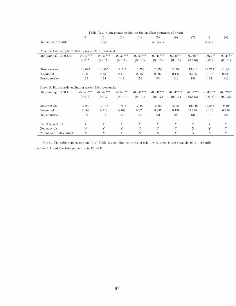
Table A65. Main results excluding the smallest countries of origin

(1) (2) (3) (4) (5) (6) (7) (8) (9)

Dependent variable pray religious service

Panel A. Full sample excluding areas>90th percentile

Dist(earthq), 1000 km -0.046*** -0.040*** -0.034*** -0.054*** -0.045*** -0.038*** -0.036** -0.029** -0.024**

(0.015) (0.011) (0.011) (0.018) (0.013) (0.013) (0.016) (0.012) (0.011)

Observations 13,692 13,595 11,245 13,753 13,656 11,294 13,811 13,713 11,344

R-squared 0.120 0.130 0.179 0.082 0.097 0.143 0.105 0.118 0.137

Org countries 159 154 143 159 154 143 159 154 143

Panel B. Full sample excluding areas>75th percentile

Dist(earthq), 1000 km -0.043*** -0.044*** -0.040** -0.049*** -0.047*** -0.042*** -0.027** -0.030** -0.029**

(0.013) (0.012) (0.015) (0.014) (0.012) (0.013) (0.013) (0.013) (0.012)

Observations 12,230 12,133 10,014 12,280 12,183 10,055 12,340 12,242 10,105

R-squared 0.106 0.116 0.166 0.074 0.087 0.130 0.098 0.110 0.126

Org countries 136 131 122 136 131 122 136 131 122

Country-year FE Y Y Y Y Y Y Y Y Y

Geo controls N Y Y N Y Y N Y Y

Parent and indl controls N N Y N N Y N N Y

Notes. The table replicates panel A of Table 5, excluding countries of origin with areas larger than the 90th percentile

in Panel A and the 75th percentile in Panel B.

87