Embed Size (px)
Citation preview

ACTS 4301
FORMULA SUMMARY
Lesson 1. Probability Review
(1) Var(X)= E[X2]- E[X]2
(2) V ar(aX + bY ) = a2V ar(X) + 2abCov(X,Y ) + b2V ar(Y )
(3) V ar(X) = V ar(X)n
Bayes’ Theorem
Pr(A|B) =Pr(B|A)Pr(A)
Pr(B)
fX(x|y) =fY (y|x)fX(x)
fY (y)
Law of total probability
If Bi is a set of exhaustive (in other words, Pr(∪iBi) = 1) and mutually exclusive (in other wordsPr(Bi ∩Bj) = 0 for i 6= j) events, then for any event A,
Pr(A) =∑i
Pr(A ∩Bi) =∑i
Pr(Bi)Pr(A|Bi)
For continuous distributions,
Pr(A) =
∫Pr(A|x)f(x)dx
Conditional Expectation Formulae
Double expectation EX [X] = EY [EX [X|Y ]]
Conditional variance V arX [X] = EY [V arX [X|Y ]] + V arY (EX [X|Y ])
Distribution, Density and Moments for Common Random Variables
Continuous Distributions
Name f(x) F (x) E[X] Var(X)
Exponential e−xθ /θ 1− e−
xθ θ θ2
Uniform on [a, b] 1b−a , x ∈ [a, b] x
θ , x ∈ [a, b] a+b2
(b−a)2
12
Gamma xα−1e−xθ /Γ(α)θα
∫ x0 f(t)dt αθ αθ2
Discrete Distributions
Bernoulli ShortcutIf a random variable can only assume two values a and b with probabilities q and 1− q respectively,then its variance is
V ar(X) = (b− a)2q(1− q)

2
Name f(x) E[X] Var(X)
Poisson e−λλx/x! λ λ
Bernoulli qx(1− q)1−x q mq(1− q)Binomial
(mx
)qx(1− q)m−x mq mq(1− q)
Lesson 2. Introduction to Long Term Insurance
Modern Insurance Contracts
1. Universal Life2. Unitized-with-profit3. Equity-linked insurance (Variable Annuity or Equity-indexed Annuity)
Underwriting Classes
1. Preferred2. Normal3. Rated4. Uninsurable
Types of Annuities
1. Single Premium Deferred Annuity (SPDA)2. Single Premium Immediate Annuity (SPIA)3. Regular Premium Deferred Annuity (RPDA)4. Joint Life Annuity5. Last Survivor Annuity6. Reversionary Annuity
Other Types of Long Term Insurance
1. Income protection insurance2. Critical illness insurance3. Long term care insurance
Forms of Ownership of Insurance Companies
1. Mutual2. Proprietary

3
Lesson 3. Survival Distributions: Probability Functions
1. Actuarial Probability Functions
tpx - probability that (x) survives t years
tqx - probability that (x) dies within t years
t|uqx - probability that (x) survives t years and then dies in the next u years.
t+upx = tpx ·u px+t
t|uqx = tpx ·u qx+t =
= tpx −t+u px =
= t+uqx −t qx2. Life Table Functions
lx is the number of lives at exact age x.dx is the number of deaths at age x which is also the number of deaths between exact age x and
exact age x+ 1.
ndx is the number of deaths between exact age x and exact age x+ n.
dx = lx − lx+1
ndx = lx − lx+n
qx = 1− px =dxlx
tpx =lx+t
lx
t|uqx =lx+t − lx+t+u
lx3. Mathematical Probability Functions
tpx = ST (x)(t) = Pr (T (x) > t)
tqx = FT (x)(t) = Pr (T (x) ≤ t)
t|uqx = Pr (t < T (x) ≤ t+ u) = FT (x)(t+ u)− FT (x)(t) =
= Pr (x+ t < X ≤ x+ t+ u|X > x) =FX(x+ t+ u)− FX(x+ t)
sX(x)
Sx+u(t) =Sx(t+ u)
Sx(u)
Sx(t) =S0(x+ t)
S0(x)
Fx(t) =F0(x+ t)− F0(x)
1− F0(x)

4
Lesson 4. Survival Distributions: Force of Mortality
µx =f0(x)
S0(x)= − d
dxlnS0(x)
µx(t) = µx+t =fx(t)
Sx(t)= − d
dtlnSx(t) = −dtpx/dt
tpx= −d lnt px
dt=dtqx/dt
tpx
Sx(t) =t px = exp
(−∫ t
0µx+s ds
)= exp
(−∫ t
0µx(s) ds
)= exp
(−∫ x+t
xµs ds
)fT (x)(t) = fx(t) =t px · µx(t) =t px · µx+t
t|uqx =
∫ t+u
tspx · µx(s) ds
tqx =
∫ t
0spx · µx(s)ds
If µ∗x(s) = µx(s) + k for 0 ≤ s ≤ t, then tp∗x = tpxe
−kt
If µx(s) = µx(s) + µx(s) for 0 ≤ s ≤ t, then tpx = tpxtpx
If µ∗x(s) = kµx(s) for 0 ≤ s ≤ t, then tp∗x = (tpx)k

5
Lesson 5. Survival Distributions: Mortality Laws
Exponential distribution or Constant Force of Mortality
µx(t) = µ
tpx = e−µt
µx+t =
{µ1, 0 < t ≤ t∗µ2, t > t∗
⇒ tpx =
{e−µ1t, 0 < t ≤ t∗e−µ1t
∗ · e−µ2(t−t∗), t > t∗
Uniform distribution or De Moivre’s law
µx(t) =1
ω − x− t, 0 ≤ t ≤ ω − x
tpx =ω − x− tω − x
, 0 ≤ t ≤ ω − x
tqx =t
ω − x, 0 ≤ t ≤ ω − x
t|uqx =u
ω − x, 0 ≤ t+ u ≤ ω − x
Beta distribution or Generalized De Moivre’s law
µx(t) =α
ω − x− t
tpx =
(ω − x− tω − x
)α, 0 ≤ t ≤ ω − x
Gompertz’s law:
µx = Bcx, c > 1
tpx = exp
(−Bc
x(ct − 1)
ln c
)Makeham’s law:
µx = A+Bcx, c > 1
tpx = exp
(−At− Bcx(ct − 1)
ln c
)Weibull Distribution
µx = kxn
S0(x) = e−kxn+1/(n+1)

6
Lesson 6. Survival Distributions: Moments
Complete Future Lifetime
ex =
∫ ∞0
ttpxµx+t dt =
∫ ∞0
tpx dt
ex =1
µfor constant force of mortality
ex =ω − x
2for uniform (de Moivre) distribution
ex =ω − xα+ 1
for generalized uniform (de Moivre) distribution
E[(T (x))2
]= 2
∫ ∞0
ttpx dt
V ar (T (x)) =1
µ2for constant force of mortality
V ar (T (x)) =(ω − x)2
12for uniform (de Moivre) distribution
V ar (T (x)) =α(ω − x)2
(α+ 1)2(α+ 2)for generalized uniform (de Moivre) distribution
n-year Temporary Complete Future Lifetime
ex:n =
∫ n
0t · tpxµx+t dt+ nnpx =
∫ n
0tpx dt
ex:n =n px(n) +n qx(n/2) for uniform (de Moivre) distribution
ex:1 = px + 0.5qx for uniform (de Moivre) distribution
ex:n =1− e−µn
µfor constant force of mortality
E[(T (x) ∧ n)2
]=
∫ ∞0
t2 ·t pxµx+t dt = 2
∫ n
0ttpx dt
Curtate Future Lifetime
ex =
∞∑k=1
kk|qx =
∞∑k=1
kpx
ex = ex − 0.5 for uniform (de Moivre) distribution
E[(K(x))2
]=∞∑k=1
k2k|qx =
∞∑k=1
(2k − 1)kpx
V ar (K(x)) = V ar (T (x))− 1
12for uniform (de Moivre) distribution

7
n-year Temporary Curtate Future Lifetime
ex:n =n−1∑k=1
kk|qx + n ·n px =n∑k=1
kpx
ex:n = ex:n − 0.5nqx for uniform (de Moivre) distribution
E[(K(x) ∧ n)2
]=
n−1∑k=1
k2k|qx + n2 ·n px =
n∑k=1
(2k − 1)kpx
Sum of Integers
n∑k=1
k =n(n+ 1)
2
n∑k=1
k2 =n(n+ 1)(2n+ 1)
6

8
Lesson 7. Survival Distributions: Percentiles and Recursions
Recursive formulas
ex = ex:n +n pxex+n
ex:n = ex:m +m pxex+m:n−m, m < n
ex = ex:n +n pxex+n = ex:n−1 +n px(1 + ex+n)
ex = px + pxex+1 = px(1 + ex+1)
ex:n = ex:m +m pxex+m:n−m =
= ex:m−1 +m px(1 + ex+m:n−m) m < n
ex:n = px + pxex+1:n−1 = px
(1 + ex+1:n−1
)Life Table Concepts
Tx =
∫ ∞0
lx+tdt, total future lifetime of a cohort of lx individuals
nLx =
∫ n
0lx+tdt, total future lifetime of a cohort of lx individuals over the next n years
Yx =
∫ ∞0
Tx+tdt
ex =Txlx
ex:n =nLxlx
Central death rate and related concepts
nmx =ndx
nLx
mx =qx
1− 0.5qxfor uniform (de Moivre) distribution
nmx = µx for constant force of mortality
a(x) =Lx − lx+1
dxthe fraction of the year lived by those dying during the year
a(x) =1
2for uniform (de Moivre) distribution

9
Lesson 8. Survival Distributions: Fractional Ages
Function Uniform Distribution of Deaths Constant Force of Mortality Hyperbolic Assumption
lx+s lx − sdx lxpsx lx+1/(px + sqx)
sqx sqx 1− psx sqx/(1− (1− s)qx)
spx 1− sqx psx px/(1− (1− s)qx)
sqx+t sqx/(1− tqx), 0 ≤ s+ t ≤ 1 1− psx sqx/(1− (1− s− t)qx)
µx+s qx/(1− sqx) − ln px qx/(1− (1− s)qx)
spxµx+s qx −psx(ln px) pxqx/(1− (1− s)qx)2
mx qx/(1− 0.5qx) − ln px q2x/(px ln px)
Lx lx − 0.5dx −dx/ ln px −lx+1 ln px/qx
ex ex + 0.5
ex:n ex:n + 0.5nqx
ex:1 px + 0.5qx

10
Lesson 9. Survival Distributions: Select Mortality
When mortality depends on the initial age as well as duration, it is known as select mortality,since the person is selected at that age. Suppose qx is a non-select or aggregate mortality andq[x]+t, t = 0, · · · , n− 1 is select mortality with selection period n. Then for all t ≥ n, q[x]+t = qx+t.

11
Lesson 10. Survival Distributions: Models for Mortality Improvement
Projected mortality for a single factor scale
q(x, t) = q(x, 0)(1− φ(x))t
Central death rate
mx =qx∫ 1
0 spx ds=
∫ 10 spxµx+s ds∫ 1
0 spx ds
Constant force of mortality between integral ages:
mx = µ
qx = 1− e−µ = 1− e−mx
mx = − ln(1− qx)
Uniform distribution between integral ages:
mx =qx∫ 1
0 (1− sqx) ds=
qx1− 0.5qx
qx =mx
1 + 0.5mxµx+0.5 = mx
Lognormal moments
E[X] = eµ+σ2/2
V ar(X) = e2µ+σ2(eσ
2 − 1)
Lee Carter model:
lm(x, t) = αx + βxKt + ε(x, t)
Usually we assume Kt is a random walk:
Kt+1 = Kt + c+ σkZt
Constraints:xω∑x=x0
βx = 1
tn∑t=t0
Kt = 0
Consequence of constraints:
αx =
∑tnt=t0
lm(x, t)
tn − t0 + 1Central death rate improvement factor:
φ(m)(x, t) = 1− m(x, t)
m(x, t− 1)
For a Lee Carter model, 1− φ(m)(x, t) is lognormal with µ = cβx and σ = βxσk.
CBD model
Logit function:lq(x, t) = ln
q(x, t)
1− q(x, t)
q(x, t) =elq(x,t)
1 + elq(x,t)
Original form of CBD model:
lq(x, t) = K(1)t +K
(2)t (x− x),
12
where x is the mean of ages in the data set.
We assume K(i)t are random walks with drift:
K(i)t+1 = K
(i)t + ci + σ
(i)k Z
(i)t ,
where Z(i)t are standard normal, Z
(1)t and Z
(2)t have fixed correlation ρ, and Z
(i)t and Z
(i)u are inde-
pendent for t 6= u.
CBD M7 model:
lq(x, t) = K(1)t +K
(2)t (x− x) +K
(3)t
((x− x)2 − s2
x
)+Gt−x,
where
s2x =
∑xmaxx=xmin
(x− x)2
xmax − xmin + 1
and K(3)t and Gt−x are time series.
For xmax − xmin even,
s2x =
n(n+ 1)
3,
where n = (xmax − xmin)/2.

13
Lesson 12. Insurance: Annual and 1/m-thly: Moments
Ax =∞∑0
k|qxvk+1 =
∞∑0
kpxqx+kvk+1
Actuarial present value under constant force and uniform (de Moivre) mortality for insurances payableat the end of the year of death
Type of insurance APV under constant force APV under uniform (de Moivre)
Whole life qq+i
aω−xω−x
n-year term qq+i (1− (vp)n)
anω−x
n-year deferred life qq+i(vp)
nvna
ω−(x+n)
ω−x
n-year pure endowment (vp)n vn(ω−(x+n))ω−x

14
Lesson 13. Insurance: Continuous - Moments - Part 1
Ax =
∫ ∞0
e−δttpxµx(t) dt
Actuarial notation for standard types of insurance
Name Present value random variable Symbol for actuarial present value
Whole life insurance vT Ax
Term life insurancevT T ≤ n0 T > n
A1x:n
Deferred whole life insurance0 T ≤ nvT T > n n|Ax
Deferred term insurance0 T ≤ nvT n < T ≤ n+m0 T > n
n|A1x:m =n |mAx
Pure endowment insurance0 T ≤ nvn T > n
A 1x:n or nEx
Endowment insurancevT T ≤ nvn T > n
Ax:n

15
Lesson 14. Insurance: Continuous - Moments - Part 2
Actuarial present value under constant force and uniform (de Moivre) mortality for insurances payableat the moment of death
Type of insurance APV under constant force APV under uniform (de Moivre)
Whole life µµ+δ
aω−xω−x
n-year term µµ+δ
(1− e−n(µ+δ)
) anω−x
n-year deferred life µµ+δe
−n(µ+δ)e−δna
ω−(x+n)
ω−x
n-year pure endowment e−n(µ+δ) e−δn(ω−(x+n))ω−x
j-th moment Multiply δ by j
in each of the above formulae
Gamma Integrands ∫ ∞0
tne−δt dt =n!
δn+1∫ u
0te−δt dt =
1
δ2
[1− (1 + δu)e−δu
]=au − uvu
δ
Variance
If Z3 = Z1 + Z2 and Z1, Z2 are mutually exclusive, then
V ar(Z3) = V ar(Z1) + V ar(Z2)− 2E[Z1]E[Z2]
16
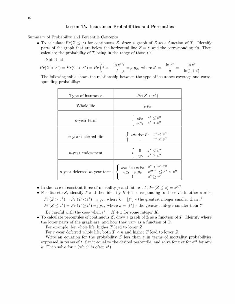
Lesson 15. Insurance: Probabilities and Percentiles
Summary of Probability and Percentile Concepts
• To calculate Pr(Z ≤ z) for continuous Z, draw a graph of Z as a function of T . Identifyparts of the graph that are below the horizontal line Z = z, and the corresponding t’s. Thencalculate the probability of T being in the range of those t’s.
Note that
Pr(Z < z∗) = Pr(vt < z∗) = Pr
(t > − ln z∗
δ
)=t∗ px, where t∗ = − ln z∗
δ= − ln z∗
ln(1 + i)
The following table shows the relationship between the type of insurance coverage and corre-sponding probability:
Type of insurance Pr(Z < z∗)
Whole life t∗px
n-year term
{npx z∗ ≤ vnt∗px z∗ > vn
n-year deferred life
{nqx +t∗ px z∗ < vn
1 z∗ ≥ vn
n-year endowment
{0 z∗ < vn
t∗px z∗ ≥ vn
n-year deferred m-year term
nqx +n+m px z∗ < vm+n
nqx +t∗ px vm+n ≤ z∗ < vn
1 z∗ ≥ vn
• In the case of constant force of mortality µ and interest δ, Pr(Z ≤ z) = zµ/δ
• For discrete Z, identify T and then identify K + 1 corresponding to those T . In other words,
Pr(Z > z∗) = Pr (T < t∗) =k qx, where k = bt∗c - the greatest integer smaller than t∗
Pr(Z ≤ z∗) = Pr (T ≥ t∗) =k px, where k = bt∗c - the greatest integer smaller than t∗
Be careful with the case when t∗ = K + 1 for some integer K.• To calculate percentiles of continuous Z, draw a graph of Z as a function of T . Identify where
the lower parts of the graph are, and how they vary as a function of T.For example, for whole life, higher T lead to lower Z.For n-year deferred whole life, both T < n and higher T lead to lower Z.Write an equation for the probability Z less than z in terms of mortality probabilities
expressed in terms of t. Set it equal to the desired percentile, and solve for t or for ekt for anyk. Then solve for z (which is often vt)

17
Lesson 16. Insurance: Recursive Formulae, Varying Insurances
Recursive Formulae
Ax = vqx + vpxAx+1
Ax = vqx + v2pxqx+1 + v22pxAx+2
Ax:n = vqx + vpxAx+1:n−1
A1x:n = vqx + vpxA
1x+1:n−1
n|Ax = vpxn−1|Ax+1
A 1x:n = vpxA
1x+1:n−1
Increasing and Decreasing Insurance
(IA)1x:n + (DA)1
x:n = (n+ 1)A1x:n(
IA)1x:n
+(DA
)1x:n
= (n+ 1)A1x:n(
IA)1x:n
+(DA
)1x:n
= nA1x:n
The Constant Force Increasing Insurance∫ ∞0
tne−δtdt =n!
δn+1∫ u
0te−δtdt =
1
δ2
(1− (1 + δu) e−δu
)=an δ − uvu
δ(IA)x
=µ
(µ+ δ)2for constant force
E[Z2] =2µ
(µ+ 2δ)3for Z a continuously increasing continuous insurance, constant force.
Recursive Formulas for Increasing and Decreasing Insurance
(IA)1x:n = A1
x:n + vpx (IA)1x+1:n−1
(IA)1x:n = A1
x:1 + vpx (IAA)1x+1:n−1
(DA)1x:n = nA1
x:1 + vpx (DA)1x+1:n−1
(DA)1x:n = A1
x:n + (DA)1x:n−1

18
Lesson 17. Relationships between Insurance Payable at Moment of Death and Payableat End of Year
Summary of formulas relating insurances payable at moment of death to insurances payable at theend of the year of death assuming uniform distribution of deaths
Ax =i
δAx
A1x:n =
i
δA1x:n
n|Ax =i
δn|Ax(
IA)1x:n
=i
δ(IA)1
x:n(ID)1x:n
=i
δ(ID)1
x:n
Ax:n =i
δA1x:n +A 1
x:n
A(m)x =
i
i(m)Ax
2Ax =2i+ i2
2δ2Ax(
IA)1x:n
=(IA)1x:n− A1
x:n
(1
d− 1
δ
)Summary of formulas relating insurances payable at moment of death to insurances payable at theend of the year of death using claims acceleration approach
Ax = (1 + i)0.5Ax
A1x:n = (1 + i)0.5A1
x:n
n|Ax = (1 + i)0.5n|Ax
Ax:n = (1 + i)0.5A1x:n +A 1
x:n
A(m)x = (1 + i)(m−1)/2mAx
2Ax = (1 + i)2Ax

19
Lesson 19. Annuities: Discrete, Expectation
Relationships between insurances and annuities
ax =1−Axd
Ax = 1− dax
ax:n =1−Ax:n
dAx:n = 1− dax:n
A1x:n = va1
x:n − a1x:n
(1 + i)Ax + iax = 1
Relationships between annuities
ax:n = an +n |axax:n = ax −n Exax+n
n|ax =n Exax+n
ax = ax:n +n |axax = ax − 1
ax:n = ax:n + 1−n Ex = ax:n−1 + 1
Other annuity equations
ax =∞∑k=0
vkkpx, ax =∞∑k=1
vkkpx
ax:n =n−1∑k=1
akk−1pxqx+k−1 + ann−1px
ax:n =
n−1∑k=0
vkkpx, ax:n =
n∑k=1
vkkpx
ax =1 + i
q + i, if qx is constant
Accumulated value
sx:n =ax:n
nExsx:n = sx+1:n−1 + 1
sx:n = sx+1:n−1 +1
n−1Ex+1
sx:n = sx:n + 1− 1
nExmthly annuities
a(m)x =
∞∑k=0
1
mvkmkm
px

20
Lesson 20. Annuities: Continuous, Expectation
Actuarial notation for standard types of annuity
Name Payment per Present value Symbol for actuarialannum at time t random variable present value
Whole life 1 t ≤ T aT ax
annuity
Temporary life1 t ≤ min(T, n)0 t > min(T, n)
aT T ≤ nan T > n
ax:n
annuity
Deferred life annuity0 t ≤ n or t > T1 n < t ≤ T
0 T ≤ naT − an T > n n|ax
Deferred temporary0 t ≤ n or t > T1 n < t ≤ n+m and t ≤ T0 T > n+m
0 T ≤ naT − an n < T ≤ n+m
an+m − an T > n+mn|ax:m
life annuity
Certain-and-life1 t ≤ max(T, n)0 t > max(T, n)
an T ≤ naT T > n
ax:n
Relationships between insurances and annuities
ax =1− Axδ
Ax = 1− δax
ax:n =1− Ax:n
δAx:n = 1− δax:n
n|ax =Ax:n − Ax
δ
General formulas for expected value
ax =
∫ ∞0
antpxµx+t dt
ax =
∫ ∞0
vttpx dt
ax:n =
∫ n
0vttpx dt
n|ax =
∫ ∞n
vttpx dt
Formulas under constant force of mortality

21
ax =1
µ+ δ
ax:n =1− e−(µ+δ)n
µ+ δ
n|ax =e−(µ+δ)n
µ+ δ
Relationships between annuities
ax = ax:n +n Exax+n
ax:n = an +n |ax

22
Lesson 21. Annuities: Variance
General formulas for second moments
E[Y 2x ] =
∫ ∞0
a2t tpxµx+t dt
E[Y 2x ] =
∞∑k=1
a2kk−1|qx
E[Y 2x:n] =
n∑k=1
a2kk−1|qx + npxa
2n =
n−1∑k=1
a2kk−1|qx + n−1pxa
2n
Special formulas for variance of whole life annuities and temporary life annuities
V ar(Yx) =2Ax − (Ax)2
δ2=
2(ax −2 ax)
δ− (ax)2
V ar(Yx:n) =2Ax:n − (Ax:n)2
δ2=
2(ax:n −2 ax:n)
δ− (ax:n)2
V ar(Yx) = V ar(Yx) =2Ax − (Ax)2
d2=
2(ax −2 ax)
d2+2 ax − (ax)2
V ar(Yx:n) = V ar(Yx:n−1) =2Ax:n − (Ax:n)2
d2
23
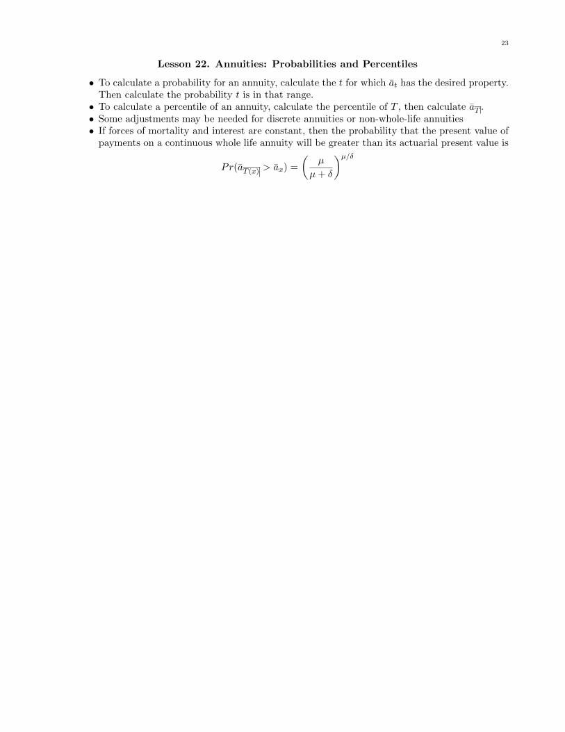
Lesson 22. Annuities: Probabilities and Percentiles
• To calculate a probability for an annuity, calculate the t for which at has the desired property.Then calculate the probability t is in that range.• To calculate a percentile of an annuity, calculate the percentile of T , then calculate aT .• Some adjustments may be needed for discrete annuities or non-whole-life annuities• If forces of mortality and interest are constant, then the probability that the present value of
payments on a continuous whole life annuity will be greater than its actuarial present value is
Pr(aT (x) > ax) =
(µ
µ+ δ
)µ/δ

24
Lesson 23. Annuities: Varying Annuities, Recursive Formulas
Increasing/Decreasing Annuities(I a)x
=1
(µ+ δ)2, if µ is constant(
I a)x:n
+(Da)x:n
= nax:n
(Ia)x:n + (Da)x:n = (n+ 1)ax:n
Recursive Formulas
Whole life annuities:
ax = vpxax+1 + 1
a(m)x = v1/m ·1/m px · a(m)
x+1/m +1
max = vpxax+1 + vpx
ax = vpxax+1 + ax:1
Temporary annuities:
ax:n = vpxax+1:n−1 + 1
ax:n = vpxax+1:n−1 + vpx
ax:n = vpxax+1:n−1 + ax:1
Deferred life annuities:
n|ax = vpx · n−1|ax+1
n|ax = vpx · n−1|ax+1
n|ax = vpx · n−1|ax+1
Certain-and-life annuities:
ax:n = 1 + vqxan−1 + vpxax+1:n−1
ax:n = v + vqxan−1 + vpxax+1:n−1
ax:n = a1 + vqxan−1 + vpxax+1:n−1

25
Lesson 24. Annuities: 1/m-thly Payments
In general:
a(m)x = a(m)
x − 1
m
1 + i =
(1 +
i(m)
m
)m=
(1− d(m)
m
)−mi(m) = m
((1 + i)
1m − 1
)d(m) = m
(1− (1 + i)−
1m
)
For small interest rates:
a(m)x ≈ ax −
m− 1
2m
a(m)x ≈ ax +
m− 1
2m
Under the uniform distribution of death (UDD) assumption:
a(m)x = ax −
m− 1
2m
a(m)x = ax +
m− 1
2m
a(m)x = α(m)ax − β(m)
a(m)x:n = α(m)ax:n − β(m)(1−n Ex)
n|a(m)x = α(m)n|ax − β(m)nEx
ax = α(∞)ax − β(∞)
a(m)x:n = a
(m)x:n −
1
m+
1
mnEx
a(m)x =
1−A(m)x
d(m)
Similar conversion formulae for converting the modal insurances to annuities hold for other types ofinsurances and annuities (only whole life version is shown).
α(m) =id
i(m)d(m)
β(m) =i− i(m)
i(m)d(m)
i(∞) = d(∞) = ln(1 + i) = δ

26
Woolhouse’s formula for approximating a(m)x :
a(m)x ≈ ax −
m− 1
2m− m2 − 1
12m2(µx + δ)
ax ≈ ax −1
2− 1
12(µx + δ)
a(m)x:n ≈ ax:n −
m− 1
2m(1−n Ex)− m2 − 1
12m2(µx + δ −n Ex(µx+n + δ))
n|a(m)x ≈n |ax −
m− 1
2mnEx −
m2 − 1
12m2 nEx(µx+n + δ)
ex = ex +1
2− 1
12µx
When the exact value of µx is not available, use the following approximation:
µx ≈ −1
2(ln px−1 + ln px)
27
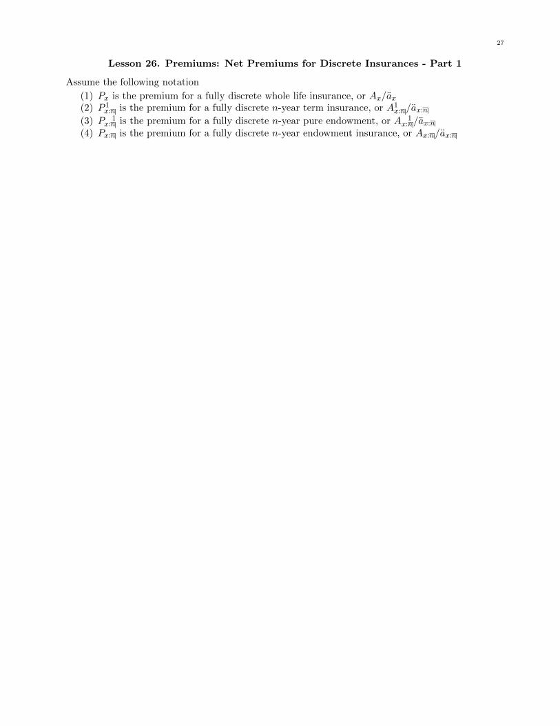
Lesson 26. Premiums: Net Premiums for Discrete Insurances - Part 1
Assume the following notation
(1) Px is the premium for a fully discrete whole life insurance, or Ax/ax(2) P 1
x:n is the premium for a fully discrete n-year term insurance, or A1x:n/ax:n
(3) P 1x:n is the premium for a fully discrete n-year pure endowment, or A 1
x:n/ax:n
(4) Px:n is the premium for a fully discrete n-year endowment insurance, or Ax:n/ax:n

28
Lesson 27. Premiums: Net Premiums for Discrete Insurances - Part 2
Whole life and endowment insurance benefit premiums
Px =1
ax− d
Px =dAx
1−Ax
Px:n =1
ax:n− d
Px:n =dAx:n
1−Ax:n
For fully discrete whole life and term insurances:If qx is constant, then Px = vqx and P 1
x:n = vqx.
Future loss at issue formulas for fully discrete whole life with face amount b:
L0 = vKx+1
(b+
Pxd
)− Px
d
E[L0] = Ax
(b+
Pxd
)− Px
d
Similar formulas are available for endowment insurances.
Refund of premium with interestTo calculate the benefit premium when premiums are refunded with interest during the deferralperiod, equate the premiums and the benefits at the end of the deferral period. Past premiums areaccumulated at interest only.
Three premium principle formulae
nPx − P 1x:n = P 1
x:nAx+n
Px:n −n Px = P 1x:n(1−Ax+n)

29
Lesson 28. Premiums: Net Premiums Paid on an 1/m-thly Basis
If premiums are payable mthly, then calculating the annual benefit premium requires dividing by anmthly annuity. If you are working with a life table having annual information only, mthly annuitiescan be estimated either by assuming UDD between integral ages or by using Woolhouse’s formula(Lesson 20). The mthly premium is then a multiple of the annual premium. For example, for h-paywhole life payable at the end of the year of death,
hP(m)x =
Ax
a(m)
x:h
=hPxax:h
a(m)
x:h

30
Lesson 29. Premiums for Fully Continuous Expectation
The equivalence principle: The actuarial present value of the benefit premiums is equal to theactuarial present value of the benefits. For instance:
whole life insurance Ax = P(Ax)ax
n− year endowment insurance Ax:n = P(Ax:n
)ax:n
n− year term insurance A 1x:n = P
(A 1x:n
)ax:n
n− year deferred insurance n|Ax =n P(n|Ax
)ax:n
n− pay whole life insurance Ax =n P(Ax)ax:n
n− year deferred annuity n|ax = P (n|ax) ax:n
P(Ax)
=1− δaxax
=1
ax− δ
P(Ax)
=Ax
(1− Ax)/δ=
δAx1− Ax
P(Ax:n
)=
1
ax:n− δ
P(Ax:n
)=
δAx:n
1− Ax:n
For constant force of mortality, P(Ax)
and P(Ax:n
)are equal to µ.
Future loss formulas for whole life with face amount b and premium amount π:
0L = bvT − πaT = bvT − π(
1− vT
δ
)= vT
(b+
π
δ
)− π
δ
E[0L] = bAx − πax = Ax
(b+
π
δ
)− π
δSimilar formulas are available for endowment insurance.
31
Lesson 30. Premiums: Gross Premiums
The gross future loss at issue Lg0 is the random variable equal to the present value at issue of benefitsplus expenses minus the present value at issue of gross premiums:
Lg0 = PV (Ben) + PV (Exp)− PV (P g)
To calculate the gross premium P g by the equivalence principle, equate P g times the annuity-due forthe premium payment period with the sum of
1. An insurance for the face amount plus settlement expenses2. P g times an annuity-due for the premium payment period of renewal percent of premium expense,
plus the excess of the first year percentage over the renewal percentage3. An annuity-due for the coverage period of the renewal per-policy and per-100 expenses, plus the
excess of first year over renewal expenses

32
Lesson 31. Premiums: Variance of Future Loss, Discrete
The following equations are for whole life and endowment insurance of 1. For whole life, drop n.
V ar(0L) =(
2Ax:n − (Ax:n)2)(
1 +P
d
)2
If equivalence principle premium is used: V ar(0L) =2Ax:n − (Ax:n)2
(1−Ax:n)2
For whole life with equivalence principle and constant force of mortality only: V ar(0L) =q(1− q)q +2 i
If the benefit is b instead of 1, and the premium P is stated per unit, multiply the variances by b2.For two whole life or endowment insurances, one with b′ units and total premium P ′ and the otherwith b units and total premium P , the relative variance of loss at issue of the first to second is((b′d+ P ′) / (bd+ P ))2.

33
Lesson 32. Premiums: Variance of Future Loss, Continuous
The following equations are for whole life and endowment insurance of 1. For whole life, drop n.
V ar(L0) =(
2Ax:n −(Ax:n
)2)(1 +
P
δ
)2
V ar(L0) =2Ax:n −
(Ax:n
)2(1− Ax:n
)2 , If equivalence principle premium is used
V ar(L0) =µ
µ+ 2δ, For whole life with equivalence principle and constant force of mortality only
For whole life and endowment insurance with face amount b:
V ar(L0) =(
2Ax −(Ax)2)(
b+P
δ
)2
V ar(L0) =(
2Ax:n −(Ax:n
)2)(b+
P
δ
)2
If the benefit is b instead of 1, and the premium P is stated per unit, multiply the variances by b2.
For two whole life or endowment insurances, one with b′ units and total premium P ′ and the otherwith b units and total premium P , the relative variance of loss at issue of the first to second is((b′δ + P ′) / (bδ + P ))2.

34
Lesson 33. Premiums: Probabilities and Percentiles of Future Loss
• For level benefit or decreasing benefit insurance, the loss at issue decreases with time for wholelife, endowment, and term insurances. To calculate the probability that the loss at issue isless than something, calculate the probabiitiy that survival time is greater than something.• For level benefit or decreasing benefit deferred insurance, the loss at issue decreases during
the deferral period, then jumps at the end of the deferral period and declines thereafter.– To calculate the probability that the loss at issue is greater then a positive number,
calculate the probability that survival time is less than something minus the probabilitythat survival time is less than the deferral period.
– To calculate the probability that the loss at issue is greater than a negative number,calculate the probability that survival time is less than something that is less than thedeferral period, and add that to the probability that survival time is less than somethingthat is greater then the deferral period minus the probability that survival time is lessthan the deferral period.
• For a deferred annuity with premiums payable during the deferral period, the loss at issuedecreases until the end of the deferral period and increases thereafter.• The 100pth percentile premium is the premium for which the loss at issue is positive with
probability p. For fully continuous whole life, this is the loss that occurs if death occurs atthe 100pth percentile of survival time.

35
Lesson 34. Premiums: Special Topics