Activity-Based Pricing in a Monopoly

V. G. Narayanan∗

Morgan HallHarvard Business SchoolBoston MA 02163.Ph 617-495-6359

E-mail: vg@hbs.edu.

February 2, 2002

Abstract

This paper studies the interaction between cost accounting systems and pricing decisionsin a setting where a monopolist sells a base product and related support services to cus-tomers whose preference for support services is known only to them. The paper considerstwo pricing mechanisms–Activity-Based Pricing (ABP) and traditional pricing, and twocost-accounting systems–Activity-Based Costing (ABC) and traditional costing. Undertraditional pricing, only the base product is priced while support services are provided freebecause detailed cost-driver volume information on the consumption of support services byeach customer is unavailable. Under ABP, customers pay based on the quantities consumedof both the base product and the support services because detailed cost-driver informationis available for each customer. Likewise, under traditional costing, the firm knows only thedistribution of the cost-driver rates for the base product and support services while underABC the firm knows the actual cost-driver rates for the base product and support services.The paper compares the equilibrium quantities of the base product and support servicessold, the information rent paid to the customers, and the expected profits of the monopolistunder all four combinations of cost-driver volume and cost-driver rate information.The paper shows that ABP helps reduce control problems, such as moral hazard and

adverse selection problems, for the supplier and increases its ability to engage in price dis-crimination. We show that firms would adopt ABP when their customer base is very diverseand the variable costs of providing customer support is high. Firms adopt ABC when theirpriors on cost-driver rates under traditional costing are very diffuse. The paper also showsthat cost-driver rate information and cost-driver volume information are complements.While prior literature has viewed ABC and Activity-Based Management (ABM) as

facilitating better decision-making, this paper shows that ABC and ABP (a form of ABM)are useful tools for addressing control problems in supply chains.

∗I thank Professors Srikant Datar, Bjorn Jorgensen, Susan Kulp and the seminar participants at the Universityof Washington and Stanford summer camp for their comments.

1 Introduction

Foster, Gupta, and Sjoblom (1996) predicted that Customer Profitability Measurement (CPM)

would be an important future direction of management accounting. There are several reasons

for this shift in focus from product profitability to customer profitability. Firms are becoming

more customer-centric rather than product-centric. When selling a portfolio of products to a

customer they use some of their products as loss leaders. They sell a mix of customized and

standardized products to the same customer. Hence, it becomes important to understand not

just product profitability, but also customer profitability.

All customer profitability measurement systems involve allocating the cost of resources

consumed in serving customers (mostly Selling, General, and Administrative costs of providing

support services) to cost pools. These costs are then allocated from cost pools to customers

using cost-drivers. For example, Owens and Minor, a distributor of medical supplies, uses the

number of Electronic Data Interchange (EDI) orders and the number of non-EDI orders as

cost drivers to allocate order processing costs to customers.1 Thus, CPM can be viewed as

an application of Activity-Based Costing (ABC) to allocate costs to customers rather than

to products. These allocated costs are then matched with revenues from each customer to

determine individual customer profitability.

In this paper, we will focus on using customer profitability information for pricing decisions

- a practice labeled Activity-Based Pricing (ABP) in the practitioner literature.2 ABP involves

harnessing the cost-driver volume and rate information, used to compute customer profitability,

to price the products and services offered to those customers. Owens and Minor, for example,

charges separately for the number of line-items in an order, the number of EDI orders, the

number of non-EDI orders, the number of deliveries, the number of emergency shipments, and

for special packaging.

This paper studies the interaction between cost accounting systems and pricing problems

in a setting where a monopolist sells a base product and related support services to cus-1See Brem and Narayanan (2000) for a complete description of the customer profitability measurement system

at Owens and Minor.2See for instance http://executiveeducationinc.com/freestuff.html.

1

tomers whose preference for support services are known only to them. The paper considers

two pricing mechanisms–Activity-Based Pricing (ABP) and traditional pricing, and two cost-

accounting systems–Activity-Based Costing (ABC) and traditional costing. Under traditional

pricing, only the base product is priced while support services are provided free because de-

tailed cost-driver volume information on the consumption of support services by each customer

is unavailable. Under ABP, customers pay for both base product and support services because

detailed cost-driver information on the volume of support services consumed by each customer

is available. Likewise, under traditional costing, the firm knows only the distribution of the

cost-driver rates for the base product and support services, while under ABC the firm knows

the actual cost-driver rates for the base product and support services. This paper compares

the equilibrium quantities of the base product and support services sold, the information rent

paid to the customers, and the expected surplus to the monopolist under all four combinations

of cost-driver volume and cost-driver rate information.

The paper shows that ABP is valuable to the seller even when the cost of providing support

services is entirely fixed and there is no uncertainty in costs. This is because contracting on

the quantity of support services helps reduce the information rent paid to the buyer. When

the cost of providing support services is variable, apart from the savings in information rent

paid to the buyer, the seller is also able to mitigate the free-rider problem in the consumption

of services. Thus, the paper shows that ABP helps reduce moral hazard and adverse selection

problems for the supplier and increases its ability to engage in price discrimination. We show

that firms would adopt ABP when their customer base is very diverse and the variable costs

of providing customer support is high.

Firms adopt ABC when their priors on cost-driver rates under traditional costing are very

diffuse. These benefits of ABP and ABC have to be traded off against the information technol-

ogy systems costs of implementing ABP and ABC. The paper also shows that cost-driver rate

information and cost-driver volume information are complements since one is more valuable in

the presence of the other.

Section 2 reviews the extant literature on customer profitability measurement, activity-

2

based costing, product bundling, and mechanism design. Section 3 presents the model. In

Section 4, we analyze several scenarios. First, a setting where the seller can observe the buyer’s

type, the quantity of goods, and the quantity of support services consumed by the buyer. This

scenario, the first-best case, serves as a useful benchmark for other scenarios. Second, a setting

labeled traditional pricing where the seller can observe only the quantity of the base product sold

to the buyer, and not the buyer’s type or consumption of support services. Finally, we consider

a setting labeled Activity-Based Pricing where the seller can contract on the consumption of

both the base product and support services by the buyer but not the buyer’s type. Both

pricing schemes are analyzed under both traditional cost accounting and activity-based cost

accounting. The section compares traditional costing and pricing with activity-based costing

and pricing, and derives conditions under which a firm might consider adopting activity-based

systems. The section quantifies the incremental value of cost-driver volume versus cost-driver

rate information. Implications for the supply chain as a whole are also examined. Section 5

concludes the paper.

2 Literature Review

This paper is related to Larsen and Narayanan (2001) who study activity-based pricing in a

duopoly. Larsen and Narayanan study the impact of one firm adopting ABP on the rival firm’s

prices and profits. They show conditions under which one firm adopting ABP results in the

other firm also adopting ABP. They find that when both firms competing in a duopoly market

adopt ABP, both firms benefit. Surprisingly, customers benefit as well. These benefits are

realized because ABP induces a better alignment of customers with firms. The firm with the

lower cost of providing customer support attracts high users of customer support and the firm

with the higher cost of providing customer support attracts the low users of customer support.

Thus, ABP serves as a screening device in Larsen and Narayanan. The insights of this paper

are more applicable when one firm has market/monopoly power while Larsen and Narayanan

is more relevant in a market with price competition. Moreover, Larsen and Narayanan do not

consider free-rider problems in the consumption of support services. Hence, we can think of

3

this paper as addressing the long-term effects of ABP where customers can adjust the quantity

of support service that they can consume, while Larsen and Narayanan models the short-term

effects of ABP where customers can only switch suppliers.

Price discrimination in the form of non-linear prices is not allowed in Larsen and Narayanan.

When customers can engage in commodity arbitrage (that is, buy the product from one supplier

and resell the product to another customer to avail of quantity discounts), the only feasible

pricing mechanism is linear pricing. Thus, the model in Narayanan and Larsen is more descrip-

tive of commodity products. Non-linear pricing, as modeled in this paper, is more descriptive

of settings where the customer cannot resell the product to other customers. All services and

manufactured products that involve customization, special packaging or shipping, and signifi-

cant freight costs would be examples of products that are not prone to commodity arbitrage.

The additional contribution of this paper over Larsen and Narayanan is to show that ABP can

be used to mitigate control problems in supply chains and to help firms with market power to

engage in better price discrimination.

This paper is also related to the economics literature on bundling, which identifies more

efficient extraction of consumer surplus as the main reason for bundling (see Stigler (1968),

Adams and Yellen (1976), Schmalensee (1984), and McAfee, McMillan, and Whinston (1989)).

When a firm has to charge one price to all customers, variability in customer valuations reduces

the seller’s ability to extract consumer surplus. Thus, bundling, which serves as a tool to reduce

heterogeneity in valuations, helps a monopolist increase profits as long as the valuations for

the products being bundled are not perfectly positively correlated.

In Section 4.2 of the paper we study traditional pricing — a form of bundled pricing where

support services are provided for free. In section 4.3 of the paper we study ABP where the base

product and support services are both priced separately. The motivation for pure bundling in

this paper is not the reduction in the variation in customer valuations of products but the

inability to price support services separately in the absence of cost-driver (activity) volume

information at the customer level to facilitate contracting. Basing the marginal price for the

base product on the level of the support service being consumed helps the firm to engage

4

in better price discrimination. Thus, the motivation for ABP in this paper is again not the

reduction in variation in customer valuations, but better price discrimination.

This paper is also related to the mechanism design literature in economics and accounting.

See Baron and Myerson (1982) for a detailed treatment of mechanism design in the context

of regulating a monopolist with unknown costs, and Tirole (1988) for a textbook treatment of

mechanism design in the context of second-degree price discrimination. We extend this litera-

ture by examining the value of an additional signal to the monopolist for price discrimination

when the monopolist sells a base product and additional support services. In the account-

ing literature, see Kirby, Reichelstein, Sen, and Paik (1991) and Melumad, Mookherjee, and

Reichelstein(1992) for applications of mechanism design concepts to study delegation and in-

centives. Our paper contributes to this literature by addressing the question–“What is the

value of an additional signal for mechanism design?” We show that the principal uses the

additional signal to reduce the information rent paid to the agent and to mitigate the agent’s

moral hazard problem.

This paper also makes a contribution to the literature on activity-based costing.3 In the

practitioner literature, Cooper and Kaplan (1988 and 1991) describe ABC and Activity-Based

Management (ABM). While there are many uses of ABC information, such as process im-

provement and new product development, this paper focuses on using ABC information for

pricing decisions. Banker and Potter (1993) compare the value of ABC for pricing decisions in

a monopoly with its value in a duopoly. They find that sometimes, ABC may not be valuable

in a duopoly setting. Banker and Potter, in contrast to this paper, study product profitability

rather than customer profitability. Moreover, the strategic interaction of the firm, in their pa-

per, is with a rival firm rather than with its customers. Banker and Hughes (1994) also study

the role of ABC information in pricing decisions by a monopolist. They find that activity-based

unit costs are relevant for pricing decisions if support activity capacities and pricing decisions

are taken simultaneously. However, they do not model a strategic interaction with customers3This paper is also related to the empirical literature on CPM. In an empirical study, Foster and Gupta (1998)

study how customer satisfaction metrics are related to customer profitability. Niraj, Gupta, and Narasimhan(1999) study customer profitability measurement in a supply chain. Narayanan and Sarkar (2000) show thatcustomer-mix decisions change when a firm adopts a CPM system as a part of an ABC system.

5

and do not consider pricing support activities separately. That is, they model traditional pric-

ing decisions based on ABC information (scenario 3 in this paper), but do not model ABP

where support activities are separately priced. However, the biggest difference between this

paper and the prior literature on ABC and ABM is the use of ABC and ABP (a form of ABM)

for control purposes rather than for decision-making.

3 The Model

We model a monopolist who sells to customers a base product and additional support services.

Customers differ in their valuation of support service and their type is indexed by the variable k.

Let q(k) be the quantity of the base product and s(k) the quantity of support service bought by

a customer of type k. Let the tariff charged by the monopolist be T (q(k), s(k), k). The utility

for customer type k from consuming quantity q of the base product and quantity s of support

services is given by φ(q, s, k) = α1q−α2q2+α3ks−α4s2+α5qs−T . We assume that reservationutility is 0 for all types of customers. Without loss of generality, we set α2 = α4 = 1.4 We

assume α1,α3 > 0 and 0 < |α5| < 2. The quadratic expression for customer utility captures thediminishing marginal utility for both the base product and support services. If α5 > 0, then

the base product and support service are complements, while they are substitutes if α5 < 0.

Support services provided to customers can be complements or substitutes for the base product.

For example, if the service is number of shipments in a month, going from two shipments a

month to four shipments could be more valuable to a customer who buys large quantities of

the base product than to a customer who buys only small quantities. However, the service of

emergency express shipments of the base product might be more valuable to a small customer

than to a large customer who might maintain his own inventory of the base product. In the

former case, the base product and support services are complements, and in the latter case,

they are substitutes.

k is assumed to be distributed with density function f(k), distribution function F (k), and4Observe that α1q − α2q

2 + α3ks− α4s2 + α5qs =

α1√α2q̃ − q̃2 + α3k√

α4s̃− s̃2 + α5

q̃s̃√α2α4

, where q̃ = q√α2 and

s̃ = s√α4.

6

support [k k]. We assume that the inverse hazard rate function h(k) ≡ 1−F (k)f(k) is decreasing in k.

That is, h0(k) ≡ dh(k)dk < 0. This property is satisfied by many distributions and is widely used

in the mechanism design literature. For example, Tirole (1988, pp.156) says, “ This property

is satisfied by many distributions, including the uniform, the normal, the Pareto, the logistic,

the exponential, and any distribution with nondecreasing density." We denote the profits of

the monopolist from customer of type k by Π(k)and revenues(tariffs) as T (q(k), s(k), k). Let

the per-unit cost of providing support services be cs, the per-unit cost of manufacturing the

base product be cq, and the total fixed cost be cf with cq, cs, cf ≥ 0. The total cost of

manufacturing the base product and providing support services is η(k) = cf+cqq(k)+css(k)+²,

where cq, cs, cf , and ² are random variables with joint density function g(cq, cs, cf , ²). Let the

expected values of cq, cs, cf , and ² be µq, µs, µf , and µ², and their variances be σ2q , σ2s ,

σ2f , and σ2² , respectively. Let the covariance between cq and cs be σq,s. When we want to

take the expectation of a function, R(cq, cs, cf , ²) with respect to cq, cs, cf , and ², we will

write Ec(R) ≡R R R R

R(c̃q, c̃s, c̃f , ²̃)g(c̃q, c̃s, c̃f , ²̃)dc̃qdc̃sdc̃fd²̃. Likewise, when we want to take

expectation of a function G(k) with respect to k, we will write Ek(G) ≡R kk G(k)f(k)dk. Let

the profitability of customer of type k be Π(k) = T (k)− η(k).

We consider two cost accounting systems–traditional and activity-based. Under ABC, the

firm observes the specific realizations of cost-driver rates cq, cs, and cf before making its pricing

decisions. Under the traditional system the firm does not. Instead, it has to base its decisions

on its knowledge of the joint distribution of cq, cs, and cf . However, the finer cost information

under ABC is not free. We assume that it costs the firm ωr to implement ABC.

Three comments about the cost systems are in order. One, it is conceivable that a firm

has a very good understanding of its cost structure and does not need an ABC system. In the

limit, if σ2q = σ2s = σ2f = σq,s = 0, the ABC system does not provide any new cost-driver rate

information. Two, if a firm knew total costs but not the break up of base-product costs and

support related costs, we would expect, σq,s < 0. Three, it is conceivable that a firm might have

pretty good priors on cq, cs, or cf , in which case we would expect their respective variances to

be small. Thus, the variance-covariance structure of the various costs captures the accuracy of

7

the traditional cost system and the potential benefits of the ABC system.

We also consider two pricing systems–traditional and activity-based. Under traditional

pricing, only the base product is priced. Support services are provided for free to the extent

demanded by the customer. Under activity-based pricing, support services are also priced.

ABP is facilitated by an accounting system that measures the cost-driver volume for each

customer. This cost-driver volume is used for contracting (i.e., pricing). We assume that it

costs ωv to implement the accounting system that provides contractible cost-driver volume

information that is necessary for activity-based pricing. Observe that the monopolist charges

a customer who consumes q units of the base product, s units of support service, and is type k,

tariff T (q, s, k). This allows for the possibility that the tariff is a function of the level of support

service supplied to the customer and the customer’s type. However, in the absence of ABP, the

tariff is independent of the level of support services supplied to the customer and T (q, s, k) =

T (q, k), ∀s. Likewise, if the customer type is not observable then T (q, s, k) = T (q, s), ∀k.Finally, if neither the customer type nor the extent of customer support is observable to the

firm, then T (q, s, k) = T (q), ∀s, k.We have chosen to present s as the quantity of support service provided to the customer.

We can also choose to interpret s as the quality or type of service provided. Consider a business

executive’s family purchasing Digital Subscriber Line service (a high-speed internet connection)

from an internet service provider. The executive might use the DSL to connect to her corporate

network at work. Her husband might use the DSL for videoconferencing, while her children

use it for interactive gaming service. If the internet service provider had the ability to track

what the DSL line is being used for, it can bill incrementally for each type of service. Cisco

recently introduced NetFlow, a Cisco software feature, to do precisely this. An article in Packet

Magazine (Third Quarter 2000) titled “Pricing for Profitability” has the following to say about

the value of NetFlow:

Service providers have typically dodged the limitations of legacy billing infrastruc-

tures by offering flat-rate pricing-thus foregoing the profitability that can be realized

from closely aligning prices with the actual value of service. To price for profitabil-

8

ity, service providers need the network to tell them what’s going on. They need

the ability to aggregate massive amounts of data and correlate it with rating infor-

mation. In short, they need usage-based accounting and billing solutions to meet

market demands.

“The current billing situation can be compared to a clothing company that doesn’t

have the means to distinguish between Oxford and plain dress shirts," says Kurt

Dahm, Senior Marketing Manager in the Communications Software group at Cisco.

Not only will the company have a hard time giving customers exactly what they

want, but it’s forced to charge the same price for all shirts, even though the shirts

have different values.

Thus, what we have called Activity-Based Pricing, Cisco has called usage-based accounting

and billing. Interpreting, s as the type of service provided, we can apply the insights of our

model to this setting.

4 Analysis

In this section, we analyze five different scenarios. In scenario 1, the firm knows its customer’s

type k, and can observe q and s. It also knows the realization of cost-driver rates before

choosing T (q(k), s(k), k). We term this the first-best case where there are no moral hazard or

adverse selection problems and no cost-driver-rate uncertainty. All endogenous variables are

subscripted f to denote the first-best case.

The following table characterizes the settings of the next four scenarios. The subscript used

to denote the endogenous variables in that scenario is given in parenthesis next to the scenario

number.

Setting Traditional Costing Activity-Based CostingTraditional Pricing Scenario 2 (t) Scenario 3 (r)Activity-Based Pricing Scenario 4 (v) Scenario 5 (a)

Table 1: Settings Analyzed

9

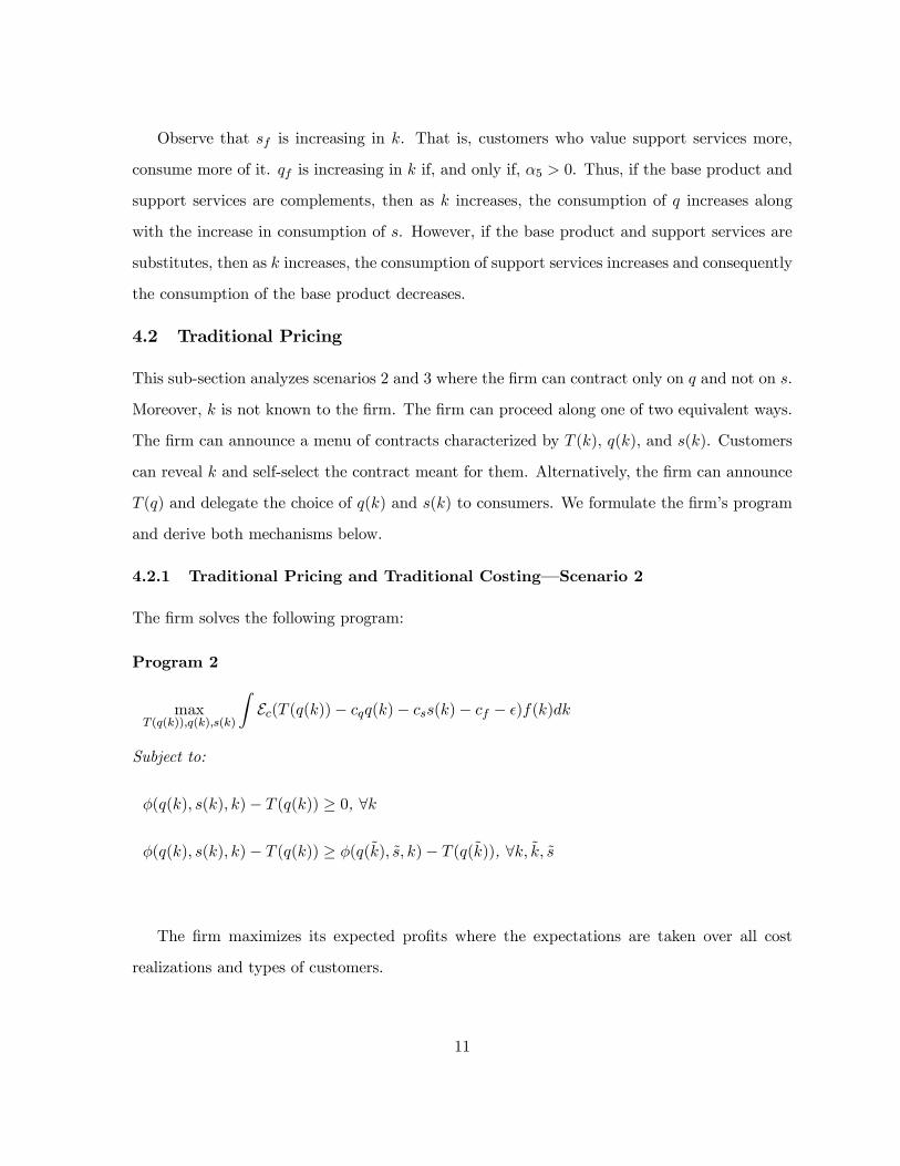
k is also unobservable in scenarios 2 through 5. Under traditional pricing, the firm can

contract only on q, while s is provided for free to the extent demanded by each customer. The

unobservability of k leads to an adverse selection problem, while the unobservability of s leads

to a moral hazard problem. We consider two cost accounting scenarios. Under traditional

costing, the firm must choose T (q) without observing the realization of cost-driver rate data.

Scenario 2 is thus traditional costing and pricing. In scenario 3, the firm has access to the

realization of cost-driver rate (ABC) information while choosing T (q). Under ABP, the firm

observes all cost-driver volume information and observes q as well as s. In this setting, there

is only an adverse selection problem. In scenario 5, the firm observes the realization of cq, cs,

cf , and ² while it does not in scenario 4.

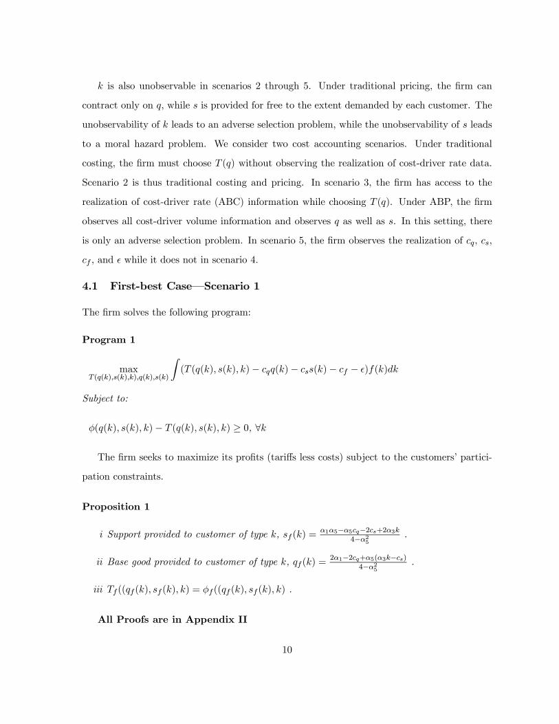
4.1 First-best Case–Scenario 1

The firm solves the following program:

Program 1

maxT (q(k),s(k),k),q(k),s(k)

Z(T (q(k), s(k), k)− cqq(k)− css(k)− cf − ²)f(k)dk

Subject to:

φ(q(k), s(k), k)− T (q(k), s(k), k) ≥ 0, ∀k

The firm seeks to maximize its profits (tariffs less costs) subject to the customers’ partici-

pation constraints.

Proposition 1

i Support provided to customer of type k, sf (k) =α1α5−α5cq−2cs+2α3k

4−α25.

ii Base good provided to customer of type k, qf (k) =2α1−2cq+α5(α3k−cs)

4−α25.

iii Tf ((qf (k), sf (k), k) = φf ((qf (k), sf (k), k) .

All Proofs are in Appendix II

10

Observe that sf is increasing in k. That is, customers who value support services more,

consume more of it. qf is increasing in k if, and only if, α5 > 0. Thus, if the base product and

support services are complements, then as k increases, the consumption of q increases along

with the increase in consumption of s. However, if the base product and support services are

substitutes, then as k increases, the consumption of support services increases and consequently

the consumption of the base product decreases.

4.2 Traditional Pricing

This sub-section analyzes scenarios 2 and 3 where the firm can contract only on q and not on s.

Moreover, k is not known to the firm. The firm can proceed along one of two equivalent ways.

The firm can announce a menu of contracts characterized by T (k), q(k), and s(k). Customers

can reveal k and self-select the contract meant for them. Alternatively, the firm can announce

T (q) and delegate the choice of q(k) and s(k) to consumers. We formulate the firm’s program

and derive both mechanisms below.

4.2.1 Traditional Pricing and Traditional Costing–Scenario 2

The firm solves the following program:

Program 2

maxT (q(k)),q(k),s(k)

ZEc(T (q(k))− cqq(k)− css(k)− cf − ²)f(k)dk

Subject to:

φ(q(k), s(k), k)− T (q(k)) ≥ 0, ∀k

φ(q(k), s(k), k)− T (q(k)) ≥ φ(q(k̃), s̃, k)− T (q(k̃)), ∀k, k̃, s̃

The firm maximizes its expected profits where the expectations are taken over all cost

realizations and types of customers.

11

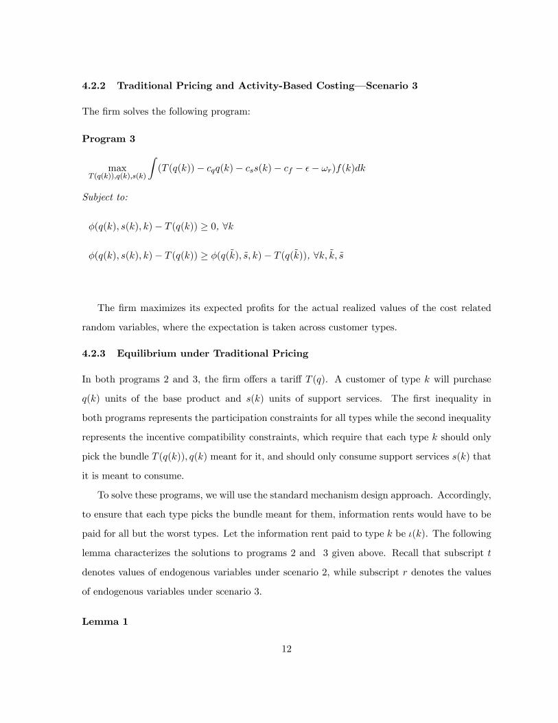
4.2.2 Traditional Pricing and Activity-Based Costing–Scenario 3

The firm solves the following program:

Program 3

maxT (q(k)),q(k),s(k)

Z(T (q(k))− cqq(k)− css(k)− cf − ²− ωr)f(k)dk

Subject to:

φ(q(k), s(k), k)− T (q(k)) ≥ 0, ∀k

φ(q(k), s(k), k)− T (q(k)) ≥ φ(q(k̃), s̃, k)− T (q(k̃)), ∀k, k̃, s̃

The firm maximizes its expected profits for the actual realized values of the cost related

random variables, where the expectation is taken across customer types.

4.2.3 Equilibrium under Traditional Pricing

In both programs 2 and 3, the firm offers a tariff T (q). A customer of type k will purchase

q(k) units of the base product and s(k) units of support services. The first inequality in

both programs represents the participation constraints for all types while the second inequality

represents the incentive compatibility constraints, which require that each type k should only

pick the bundle T (q(k)), q(k) meant for it, and should only consume support services s(k) that

it is meant to consume.

To solve these programs, we will use the standard mechanism design approach. Accordingly,

to ensure that each type picks the bundle meant for them, information rents would have to be

paid for all but the worst types. Let the information rent paid to type k be ι(k). The following

lemma characterizes the solutions to programs 2 and 3 given above. Recall that subscript t

denotes values of endogenous variables under scenario 2, while subscript r denotes the values

of endogenous variables under scenario 3.

Lemma 1

12

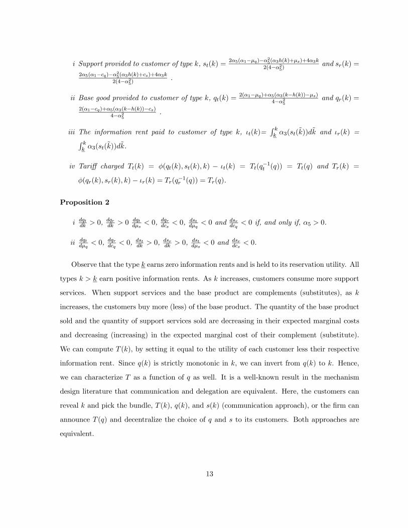
i Support provided to customer of type k, st(k) =2α5(α1−µq)−α25(α3h(k)+µs)+4α3k

2(4−α25)and sr(k) =

2α5(α1−cq)−α25(α3h(k)+cs)+4α3k2(4−α25)

.

ii Base good provided to customer of type k, qt(k) =2(α1−µq)+α5(α3(k−h(k))−µs)

4−α25and qr(k) =

2(α1−cq)+α5(α3(k−h(k))−cs)4−α25

.

iii The information rent paid to customer of type k, ιt(k)=R kk α3(st(k̃))dk̃ and ιr(k) =R k

k α3(st(k̃))dk̃.

iv Tariff charged Tt(k) = φ(qt(k), st(k), k) − ιt(k) = Tt(q−1t (q)) = Tt(q) and Tr(k) =

φ(qr(k), sr(k), k)− ιr(k) = Tr(q−1r (q)) = Tr(q).

Proposition 2

i dqtdk > 0,

dqrdk > 0

dqtdµs

< 0, dqrdcs < 0,dstdµq

< 0 and dsrdcq

< 0 if, and only if, α5 > 0.

ii dqtdµq

< 0, dqrdcq < 0,dstdk > 0,

dsrdk > 0,

dstdµs

< 0 and dsrdcs< 0.

Observe that the type k earns zero information rents and is held to its reservation utility. All

types k > k earn positive information rents. As k increases, customers consume more support

services. When support services and the base product are complements (substitutes), as k

increases, the customers buy more (less) of the base product. The quantity of the base product

sold and the quantity of support services sold are decreasing in their expected marginal costs

and decreasing (increasing) in the expected marginal cost of their complement (substitute).

We can compute T (k), by setting it equal to the utility of each customer less their respective

information rent. Since q(k) is strictly monotonic in k, we can invert from q(k) to k. Hence,

we can characterize T as a function of q as well. It is a well-known result in the mechanism

design literature that communication and delegation are equivalent. Here, the customers can

reveal k and pick the bundle, T (k), q(k), and s(k) (communication approach), or the firm can

announce T (q) and decentralize the choice of q and s to its customers. Both approaches are

equivalent.

13

It is instructive to compare the equilibria characterized above with the equilibrium in the

first-best case. In the first-best case, the firm has no moral hazard problem in the consumption

of support services, and customers have no private information.

Proposition 3

i Ec(st − sf ) = Ec(sr − sf ) = µs2 −

α25α3h(k)

2(4−α25)

ii Ec(qt − qf ) = Ec(qr − qf ) = −α5α3h(k)4−α25

Comparing the expected consumption of support services for each customer under tra-

ditional costing with that under the first-best case, we see that there are two factors that

determine the difference between them. Since support services are not priced (that is T is not

dependent of s), there is a free-rider problem under traditional pricing and customers consume

more support services relative to the first-best case. As the expected unit cost of support

services µs increases, the free-rider problem gets worse. If µs = 0, then there is no free-rider

problem as it costs the firm nothing to provide all the support that is required by the cus-

tomer. That would be the case when all support related costs are fixed. The other factor is

the distortion in the consumption of support services induced by the firm to prevent the higher

k types from choosing the bundle meant for the lower k types. The firm accomplishes this by

reducing the support services meant for the lower k types. Observe that for the highest type

k, h(k) = 0, and there is no distortion induced. Also note that the distortions, relative to the

first-best case, on account of adverse selection and moral hazard go in opposite directions.

It might seem counter-intuitive that the firm can reduce the supply of support service to

its customers when it cannot even observe how much support service they consume. The way

this reduction in supply is accomplished is subtle. The firm reduces (increases) the supply of

the base product when the base product and support services are complements (substitutes).

This is the intuition behind Proposition 3(ii).

From Proposition 3 we see that Ec(st) = Ec(sr) and Ec(qt) = Ec(qr). Hence, Ec(ιt − ιr) = 0.

Since there is no difference in expected information rent or the consumption of the base product

or support services between Scenario 2 and Scenario 3 for any customer, it might be tempting

14

to conclude that cost-driver rate information has no value. As the following proposition shows,

this conclusion is incorrect.

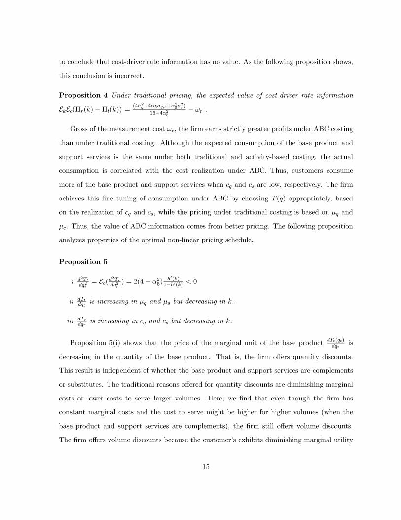
Proposition 4 Under traditional pricing, the expected value of cost-driver rate information

EkEc(Πr(k)−Πt(k)) = (4σ2q+4α5σq,s+α25σ

2s)

16−4α25− ωr .

Gross of the measurement cost ωr, the firm earns strictly greater profits under ABC costing

than under traditional costing. Although the expected consumption of the base product and

support services is the same under both traditional and activity-based costing, the actual

consumption is correlated with the cost realization under ABC. Thus, customers consume

more of the base product and support services when cq and cs are low, respectively. The firm

achieves this fine tuning of consumption under ABC by choosing T (q) appropriately, based

on the realization of cq and cs, while the pricing under traditional costing is based on µq and

µc. Thus, the value of ABC information comes from better pricing. The following proposition

analyzes properties of the optimal non-linear pricing schedule.

Proposition 5

i d2Ttdq2t

= Ec(d2Trdq2r) = 2(4− α25)

h0(k)1−h0(k) < 0

ii dTtdqt

is increasing in µq and µs but decreasing in k.

iii dTrdqr

is increasing in cq and cs but decreasing in k.

Proposition 5(i) shows that the price of the marginal unit of the base product dTt(qt)dqt

is

decreasing in the quantity of the base product. That is, the firm offers quantity discounts.

This result is independent of whether the base product and support services are complements

or substitutes. The traditional reasons offered for quantity discounts are diminishing marginal

costs or lower costs to serve larger volumes. Here, we find that even though the firm has

constant marginal costs and the cost to serve might be higher for higher volumes (when the

base product and support services are complements), the firm still offers volume discounts.

The firm offers volume discounts because the customer’s exhibits diminishing marginal utility

15

for the base product. The extent of volume discounts is affected by the firm’s adverse selection

problem. If, and only if, d2h(k)dk2

< 0, the firm increases the volume discount as the customer’s

type increases.

Propostions 5(ii) and 5(iii) show how the marginal price charged by the firm is affected by

various parameters. Thus, when the marginal cost of the base product µq increases, we know

from Proposition 2 that the quantity of the base product supplied decreases. This decrease is

accomplished by an increase in the marginal price charged to customers. Proposition 5 also

makes it clear that under ABC the firm can respond to the actual realized value of cq and cs

when setting prices, while under traditional costing prices are set based on µq and µs.

However, ABC information does not come for free. There is a cost of ωr to implement

ABC. Although this paper considers only a one-period model, an ABC system once installed

will probably give valid cost signals for several periods till the production environment of the

firm changes. Likewise, a firm that does not adopt ABC can use the realized aggregate values

of cost-driver volumes at the end of each period to update its priors on the distribution of

cost-driver rates. Appendix I considers a two-period model. The firm can choose an ABC

system or a traditional costing system at the beginning of the first period. If it adopts an ABC

system, it enjoys the benefits of finer cost information for both periods. If the firm adopts a

traditional costing system, it updates its priors on cost-driver rates at the end of the first period

based on the total cost-driver volume information that it observes at the firm level (Ek(q(k))and Ek(s(k)). To make the updating process tractable, cost-driver rates are assumed to bedistributed multivariate normal in Appendix I.

The main insight from Appendix I is that the marginal price in the second period is in-

creasing in the first period’s total cost realization, even though the total cost includes fixed

cost cf . The firm’s second period pricing decisions are influenced by first period total costs

because the first period’s total cost realization is informative about the marginal costs of the

second period. The appendix also shows that the benefits of ABC are strictly less in the second

period compared to the first period. Moreover, firms are less likely to adopt ABC if σ² and σf

are low. Thus, the one-period model may overstate the value of ABC by overlooking the firm’s

16

ability to learn more about its cost cost-driver rates by observing the prior period’s total cost

realization and aggregate cost-driver volume information. This is particularly true if the firm

has tight priors on its cost-driver rates and its total cost is not subject to much random noise.

4.3 Activity-Based Pricing

This subsection considers the case where the firm can contract on both q and s. We present

two programs– one under traditional costing and one under activity-based costing.

4.3.1 Activity-Based Pricing and Traditional Costing–Scenario 4

The firm solves the following program:

Program 4

maxT (q(k),s(k)),q(k),s(k)

Z(Ec(T (k)− cqq(k)− css(k)− cf − ²− ωv))f(k)dk

Subject to:

φ(q(k), s(k), k)− T (k) ≥ 0, ∀k

φ(q(k), s(k), k)− T (k) ≥ φ(q(k̃), s(k̃), k), k)− T (k̃), ∀k, k̃

4.3.2 Activity-Based Pricing and Activity-Based Costing–Scenario 5

The firm solves the following program:

Program 5

maxT (q(k),s(k)),q(k),s(k)

Z(T (k)− cqq(k)− css(k)− cf − ²− ωr − ωv)f(k)dk

Subject to:

φ(q(k), s(k), k)− T (k) ≥ 0, ∀k

φ(q(k), s(k), k)− T (k) ≥ φ(q(k̃), s(k̃), k), k)− T (k̃), ∀k, k̃

17

In both programs 4 and 5, the firm offers a bundle T (k), q(k),s(k). A customer of type k will

purchase q(k) units of the base product and s(k) units of support services. In both programs,

the first constraint is the participation constraint for all types while the second constraint is the

incentive compatibility constraint that each type k should only pick the bundle T (k),q(k),s(k)

meant for it.

4.3.3 Equilibrium under Activity-Based Pricing

The following lemma characterizes the solution to the programs given above. Recall that we

subscript endogenous variables with v for the activity-based pricing under traditional costing,

and with a for activity-based pricing under activity-based costing.

Lemma 2

i Support provided to customer of type k, sv(k) =α5(α1−µq)−2(α3(h(k)−k)+µs)

(4−α25)and sa(k) =

α5(α1−cq)−2(α3(h(k)−k)+cs)(4−α25)

.

ii Base good provided to customer of type k, qv(k) =2(α1−µq)+α5(α3(k−h(k))−µs)

4−α25and qa(k) =

2(α1−cq)+α5(α3(k−h(k))−cs)4−α25

.

iii The information rent paid to customer of type k, ιv(k)=R kk α3(sv(k̃))dk̃ and ιa(k) =R k

k α3(sa(k̃))dk̃ .

iv Tariff charged Tv(k) = φ(qv(k), sv(k), k)− ιv(k) and Ta(k) = φ(qa(k), sa(k), k)− ιa(k) .

Note that all the comparative statics results in Proposition 2 for traditional pricing hold for

ABP as well with the subscripts v and a substituted for t and r, respectively. Note also that

the lemma above characterizes the mechanism involving communication of k. An equivalent

mechanism where the firm announces T (q, s) and customers are delegated the choice of q(k)

and s(k) can also be solved for.5 The following Proposition compares q and s under ABP and

the first-best case.5To observe this, note that sa(k) is monotone increasing in k and is thus invertible. We have two differential

equations from the customer optimization δTδq= α1 − 2q + α5s and δT

δs= α3k − 2s + α5q. From these two

equations, T (q, s) =R s0α3s

−1a (s̃)ds̃− s2 + α5qs+ α1q − q2 + θ. The constant of integration θ, can be solved for

from the fact that the lowest type k earns no information rent and Ta(k) = φ(qa(k), sa(k), k).

18

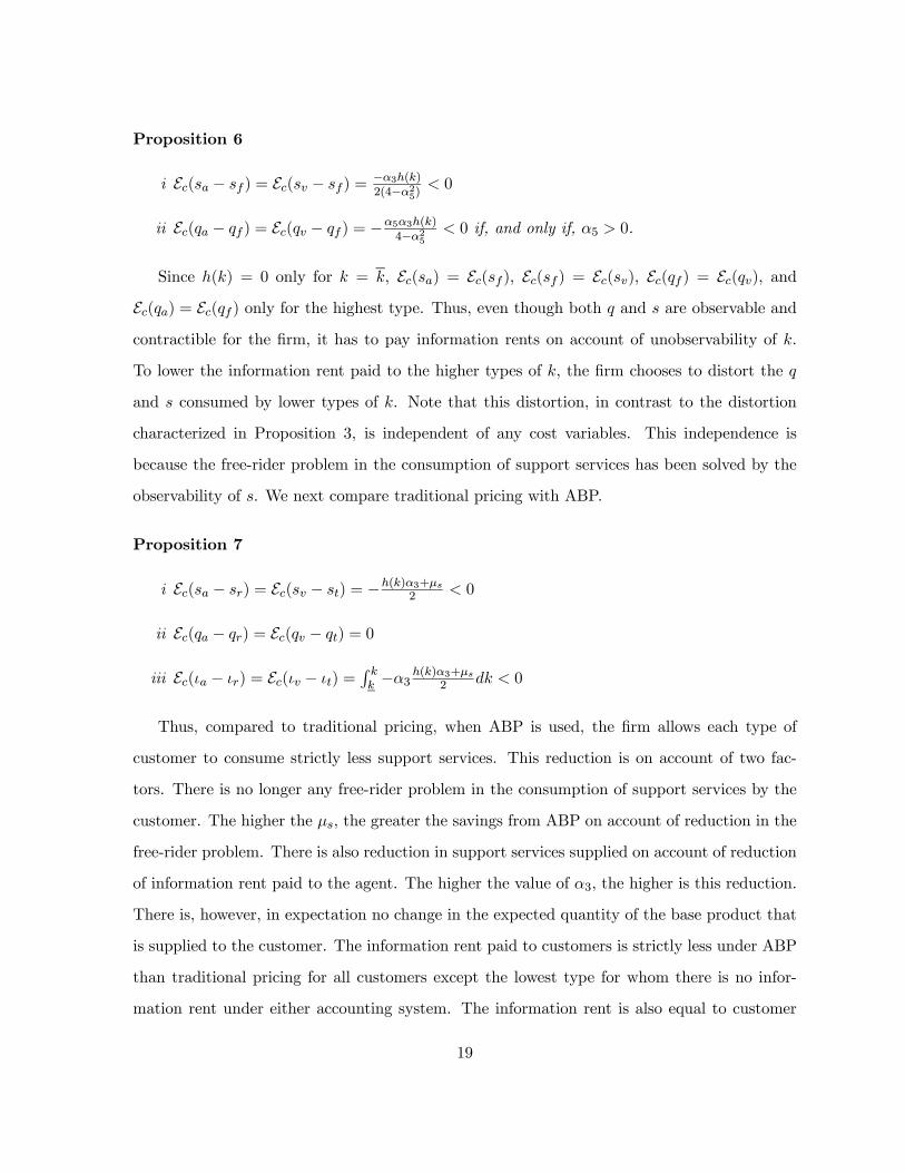
Proposition 6

i Ec(sa − sf ) = Ec(sv − sf ) = −α3h(k)2(4−α25)

< 0

ii Ec(qa − qf ) = Ec(qv − qf ) = −α5α3h(k)4−α25

< 0 if, and only if, α5 > 0.

Since h(k) = 0 only for k = k, Ec(sa) = Ec(sf ), Ec(sf ) = Ec(sv), Ec(qf ) = Ec(qv), andEc(qa) = Ec(qf ) only for the highest type. Thus, even though both q and s are observable andcontractible for the firm, it has to pay information rents on account of unobservability of k.

To lower the information rent paid to the higher types of k, the firm chooses to distort the q

and s consumed by lower types of k. Note that this distortion, in contrast to the distortion

characterized in Proposition 3, is independent of any cost variables. This independence is

because the free-rider problem in the consumption of support services has been solved by the

observability of s. We next compare traditional pricing with ABP.

Proposition 7

i Ec(sa − sr) = Ec(sv − st) = −h(k)α3+µs2 < 0

ii Ec(qa − qr) = Ec(qv − qt) = 0

iii Ec(ιa − ιr) = Ec(ιv − ιt) =R kk −α3 h(k)α3+µs2 dk < 0

Thus, compared to traditional pricing, when ABP is used, the firm allows each type of

customer to consume strictly less support services. This reduction is on account of two fac-

tors. There is no longer any free-rider problem in the consumption of support services by the

customer. The higher the µs, the greater the savings from ABP on account of reduction in the

free-rider problem. There is also reduction in support services supplied on account of reduction

of information rent paid to the agent. The higher the value of α3, the higher is this reduction.

There is, however, in expectation no change in the expected quantity of the base product that

is supplied to the customer. The information rent paid to customers is strictly less under ABP

than traditional pricing for all customers except the lowest type for whom there is no infor-

mation rent under either accounting system. The information rent is also equal to customer

19

surplus (customer utility less tariffs paid to the firm). Thus, customer surplus is strictly less

under ABP for all types of customers other than the lowest type, who earns no surplus under

either accounting system.

We next turn to the question of which type of customer is the most profitable for the firm

under the various scenarios.

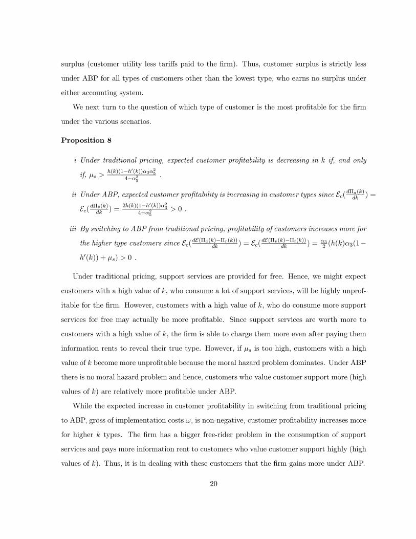
Proposition 8

i Under traditional pricing, expected customer profitability is decreasing in k if, and only

if, µs >h(k)(1−h0(k))α3α25

4−α25.

ii Under ABP, expected customer profitability is increasing in customer types since Ec(dΠa(k)dk ) =

Ec(dΠv(k)dk ) =2h(k)(1−h0(k))α23

4−α25> 0 .

iii By switching to ABP from traditional pricing, profitability of customers increases more for

the higher type customers since Ec(dE(Πa(k)−Πr(k))dk ) = Ec(dE(Πv(k)−Πt(k))dk ) = α32 (h(k)α3(1−

h0(k)) + µs) > 0 .

Under traditional pricing, support services are provided for free. Hence, we might expect

customers with a high value of k, who consume a lot of support services, will be highly unprof-

itable for the firm. However, customers with a high value of k, who do consume more support

services for free may actually be more profitable. Since support services are worth more to

customers with a high value of k, the firm is able to charge them more even after paying them

information rents to reveal their true type. However, if µs is too high, customers with a high

value of k become more unprofitable because the moral hazard problem dominates. Under ABP

there is no moral hazard problem and hence, customers who value customer support more (high

values of k) are relatively more profitable under ABP.

While the expected increase in customer profitability in switching from traditional pricing

to ABP, gross of implementation costs ω, is non-negative, customer profitability increases more

for higher k types. The firm has a bigger free-rider problem in the consumption of support

services and pays more information rent to customers who value customer support highly (high

values of k). Thus, it is in dealing with these customers that the firm gains more under ABP.

20

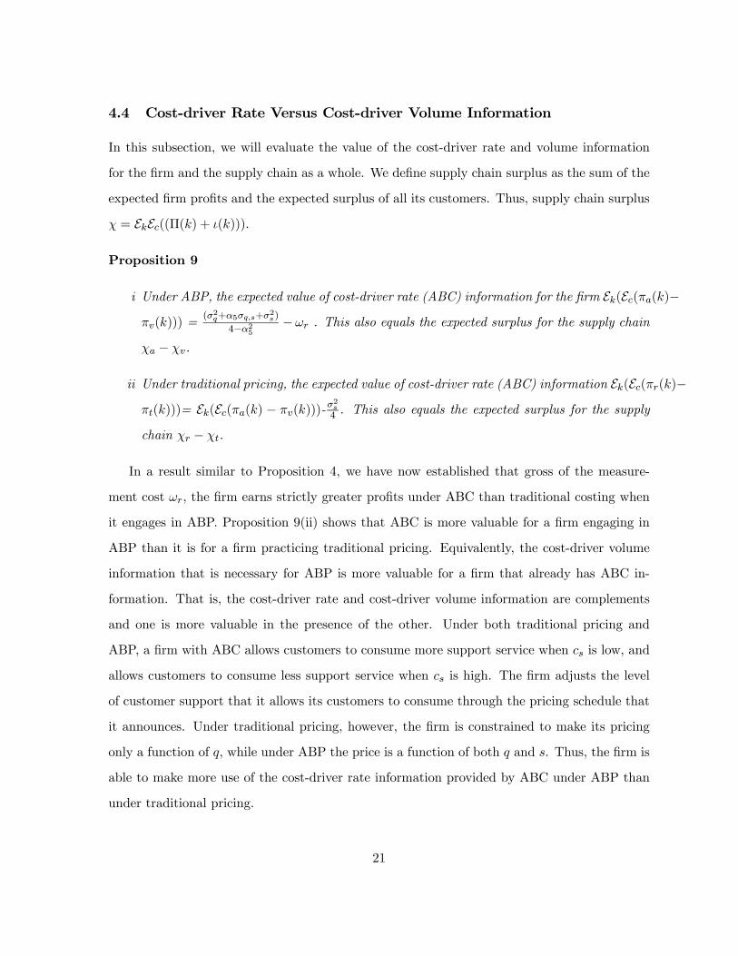
4.4 Cost-driver Rate Versus Cost-driver Volume Information

In this subsection, we will evaluate the value of the cost-driver rate and volume information

for the firm and the supply chain as a whole. We define supply chain surplus as the sum of the

expected firm profits and the expected surplus of all its customers. Thus, supply chain surplus

χ = EkEc((Π(k) + ι(k))).

Proposition 9

i Under ABP, the expected value of cost-driver rate (ABC) information for the firm Ek(Ec(πa(k)−πv(k))) =

(σ2q+α5σq,s+σ2s)

4−α25−ωr . This also equals the expected surplus for the supply chain

χa − χv.

ii Under traditional pricing, the expected value of cost-driver rate (ABC) information Ek(Ec(πr(k)−πt(k)))= Ek(Ec(πa(k) − πv(k)))-

σ2s4 . This also equals the expected surplus for the supply

chain χr − χt.

In a result similar to Proposition 4, we have now established that gross of the measure-

ment cost ωr, the firm earns strictly greater profits under ABC than traditional costing when

it engages in ABP. Proposition 9(ii) shows that ABC is more valuable for a firm engaging in

ABP than it is for a firm practicing traditional pricing. Equivalently, the cost-driver volume

information that is necessary for ABP is more valuable for a firm that already has ABC in-

formation. That is, the cost-driver rate and cost-driver volume information are complements

and one is more valuable in the presence of the other. Under both traditional pricing and

ABP, a firm with ABC allows customers to consume more support service when cs is low, and

allows customers to consume less support service when cs is high. The firm adjusts the level

of customer support that it allows its customers to consume through the pricing schedule that

it announces. Under traditional pricing, however, the firm is constrained to make its pricing

only a function of q, while under ABP the price is a function of both q and s. Thus, the firm is

able to make more use of the cost-driver rate information provided by ABC under ABP than

under traditional pricing.

21

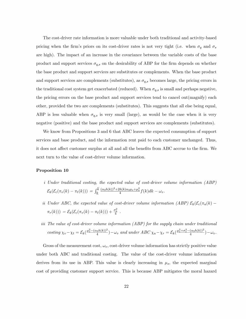
The cost-driver rate information is more valuable under both traditional and activity-based

pricing when the firm’s priors on its cost-driver rates is not very tight (i.e. when σq and σs

are high). The impact of an increase in the covariance between the variable costs of the base

product and support services σq,s on the desirability of ABP for the firm depends on whether

the base product and support services are substitutes or complements. When the base product

and support services are complements (substitutes), as σq,s becomes large, the pricing errors in

the traditional cost system get exacerbated (reduced). When σq,s is small and perhaps negative,

the pricing errors on the base product and support services tend to cancel out(magnify) each

other, provided the two are complements (substitutes). This suggests that all else being equal,

ABP is less valuable when σq,s is very small (large), as would be the case when it is very

negative (positive) and the base product and support services are complements (substitutes).

We know from Propositions 3 and 6 that ABC leaves the expected consumption of support

services and base product, and the information rent paid to each customer unchanged. Thus,

it does not affect customer surplus at all and all the benefits from ABC accrue to the firm. We

next turn to the value of cost-driver volume information.

Proposition 10

i Under traditional costing, the expected value of cost-driver volume information (ABP)

Ek(Ec(πv(k)− πt(k))) =R kk(α3h(k))2+2h(k)α3µs+µ2s

4 f(k)dk − ωv.

ii Under ABC, the expected value of cost-driver volume information (ABP) Ek(Ec(πa(k) −πr(k))) = Ek(Ec(πv(k)− πt(k))) +

σ2s4 .

iii The value of cost-driver volume information (ABP) for the supply chain under traditional

costing χv−χt = Ek(µ2s−(α3h(k))2

4 )−ωv and under ABC χa−χr = Ek(µ2s+σ

2s−(α3h(k))24 )−ωv.

Gross of the measurement cost, ωv, cost-driver volume information has strictly positive value

under both ABC and traditional costing. The value of the cost-driver volume information

derives from its use in ABP. This value is clearly increasing in µs, the expected marginal

cost of providing customer support service. This is because ABP mitigates the moral hazard

22

problem in the consumption of support services. Hence, the greater the cost of providing

support services, the greater the value of ABP. As seen in Proposition 9(ii), the cost-driver

volume information is more valuable for a firm that already has cost-driver rate information.

Moreover, this incremental value of ABP under ABC relative to its value under traditional

costing is increasing in σs. That is, the more diffuse the firm’s priors are under traditional

costing about its cost to serve its customers, the greater the incremental value of ABP under

ABC relative to traditional costing.

The impact of ABP on supply chain surplus is ambiguous. The reduction in moral hazard

helps the supply chain. More efficient price discrimination by the firm under ABP results in

the distortion in consumption of support services by customers. This distortion hurts customer

and supply chain surplus. The net effect of the moral hazard reduction and increased price

discrimination on supply chain surplus could go in either direction.

To obtain greater insight into the value of ABP, we consider the case where k has a uniform

distribution.

Proposition 11 When k is distributed uniform [µk − σk, µk + σk]

i Under traditional costing, the expected value of cost-driver volume information (ABP)

Ek(Ec(πv(k)− πt(k))) =3σ2s+3µ

2s+6µsα3σk+4α

23σ

2k

12 − ωv.

ii Under ABC, the expected value of cost-driver volume information (ABP) Ek(Ec(πa(k) −πr(k))) = Ek(Ec(πv(k)− πt(k))) +

σ2s4 .

iii d(E(Πa)−E(Πr))dσk

= d(E(Πv)−E(Πt))dσk

= α3µs2 +

2α23σk3 > 0.

iv d(E(Πa)−E(Πr))dµk

= d(E(Πv)−E(Πt))dµk

= 0.

v The value of cost-driver volume information (ABP) for the supply chain under traditional

costing χv − χt =µ2s4 − (α3σk)

2

3 − ωv and under ABC χa − χr =µ2s4 − (α3σk)

2

3 + σ2s4 − ωv.

From Proposition 11 we can see that in the case of the uniform distribution, the value

of ABP for the firm under both ABC and traditional costing is increasing in the diversity of

23

customer types (as measured by σk), but is not affected by the average preference for support

services (µk). The value of ABP for the supply chain however is decreasing in the diversity

of customer types. Thus, if σk is high, ABP becomes very attractive to the firm but ends up

hurting the overall supply chain.

5 Conclusions

Although the concepts of CPM and ABP are not new, they appear to have become more pop-

ular recently because they are IT intensive, and IT costs of implementing them have declined

dramatically in the last few years. Firms that have implemented Customer Relationship Man-

agement and Enterprise Resource Planning database systems find it easy to implement ABP

because they already have the cost-driver volume data.

In this paper, we show how and when activity-based costing and activity-based pricing are

useful in contracting with customers who buy a base product and support services. As might

be expected, ABC helps the firm price its products and services better. Perhaps less apparent,

ABP also helps reduce the information rent paid to customers and their free riding on support

services. Moreover, after the adoption of ABP, high users of customer support become the

most profitable customers for the firm. We show that ABP is more useful to the firm when the

costs associated with support services are more variable, and when the “types” of customers

the firm deals with are highly diverse. ABC is more useful when the firm’s priors about its

costs are not very tight. The firm has to tradeoff these benefits of ABP and ABC against their

respective implementation costs.

We show that it is the cost-driver volume information, rather than the cost-driver rate

information that helps the firm improve its price discrimination and mitigate customer moral

hazard. Cost-driver rate information on the other hand, is useful for selecting the appropriate

quantity of the base product and support services through an appropriate choice of prices.

However, the cost-driver rate information and cost-driver volume information are complements

and the marginal value of one increases with the availability of the other.

It has been shown in prior literature that the firm’s ability to engage in price discrimination

24

is reduced, although not eliminated, in the presence of competition.6 Moreover, the firm’s

ability to mitigate its customer’s moral hazard problem and its ability to price its products

appropriately would be valuable even in a competitive setting. Thus, we would expect many

of the insights from this paper to hold in competitive settings as well. What is an open and

interesting research question is how well a firm can use prices in an competitive market setting

to infer information about its own costs without investing in an expensive ABC information to

estimate its cost-driver rates. We leave that question for future research.

6See Stole(1995).

25

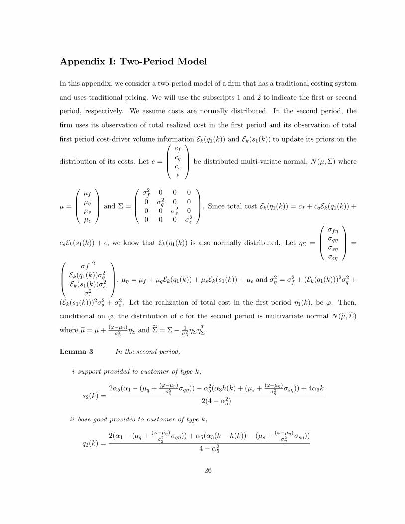
Appendix I: Two-Period Model

In this appendix, we consider a two-period model of a firm that has a traditional costing system

and uses traditional pricing. We will use the subscripts 1 and 2 to indicate the first or second

period, respectively. We assume costs are normally distributed. In the second period, the

firm uses its observation of total realized cost in the first period and its observation of total

first period cost-driver volume information Ek(q1(k)) and Ek(s1(k)) to update its priors on the

distribution of its costs. Let c =

cfcqcs²

be distributed multi-variate normal, N(µ,Σ) where

µ =

µfµqµsµ²

and Σ =

σ2f 0 0 0

0 σ2q 0 0

0 0 σ2s 00 0 0 σ2²

. Since total cost Ek(η1(k)) = cf + cqEk(q1(k)) +

csEk(s1(k)) + ², we know that Ek(η1(k)) is also normally distributed. Let ηΣ =

σfησqησsησ²η

=

σf 2

Ek(q1(k))σ2qEk(s1(k))σ2s

σ2²

, µη = µf + µqEk(q1(k)) + µsEk(s1(k)) + µ² and σ2η = σ2f + (Ek(q1(k)))2σ2q +

(Ek(s1(k)))2σ2s + σ2² . Let the realization of total cost in the first period η1(k), be ϕ. Then,

conditional on ϕ, the distribution of c for the second period is multivariate normal N(eµ, eΣ)where eµ = µ+ (ϕ−µη)

σ2ηηΣ and eΣ = Σ− 1

σ2ηηΣη

T

Σ.

Lemma 3 In the second period,

i support provided to customer of type k,

s2(k) =2α5(α1 − (µq + (ϕ−µη)

σ2ησqη))− α25(α3h(k) + (µs +

(ϕ−µη)σ2η

σsη)) + 4α3k

2(4− α25)

ii base good provided to customer of type k,

q2(k) =2(α1 − (µq + (ϕ−µη)

σ22σqη)) + α5(α3(k − h(k))− (µs + (ϕ−µη)

σ2ησsη))

4− α25

26

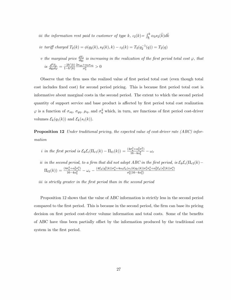
iii the information rent paid to customer of type k, ι2(k)=R kk α3s2(k̃)dk̃

iv tariff charged T2(k) = φ(q2(k), s2(k), k)− ι2(k) = T2(q−12 (q)) = T2(q)

v the marginal price dT2dq2

is increasing in the realization of the first period total cost ϕ, that

is d2T2dq2dϕ

= −2h0(k)1−h0(k)

2σqη+α5σsησ2η

> 0

Observe that the firm uses the realized value of first period total cost (even though total

cost includes fixed cost) for second period pricing. This is because first period total cost is

informative about marginal costs in the second period. The extent to which the second period

quantity of support service and base product is affected by first period total cost realization

ϕ is a function of σsη, σqη, µη, and σ2η which, in turn, are functions of first period cost-driver

volumes Ek(q1(k)) and Ek(s1(k)).

Proposition 12 Under traditional pricing, the expected value of cost-driver rate (ABC) infor-

mation

i in the first period is EkEc(Πr1(k)−Πt1(k)) = (4σ2q+α25σ

2s)

16−4α25− ωr

ii in the second period, to a firm that did not adopt ABC in the first period, is EkEc(Πr2(k)−Πt2(k)) =

(4σ2q+α25σ

2s)

16−4α25− ωr − (4Ek(q21(k))σ4q+4α5Ek(s1(k)q1(k))σ2sσ2q+α25Ek(s21(k))σ4s)

σ2η(16−4α25)

iii is strictly greater in the first period than in the second period

Proposition 12 shows that the value of ABC information is strictly less in the second period

compared to the first period. This is because in the second period, the firm can base its pricing

decision on first period cost-driver volume information and total costs. Some of the benefits

of ABC have thus been partially offset by the information produced by the traditional cost

system in the first period.

27

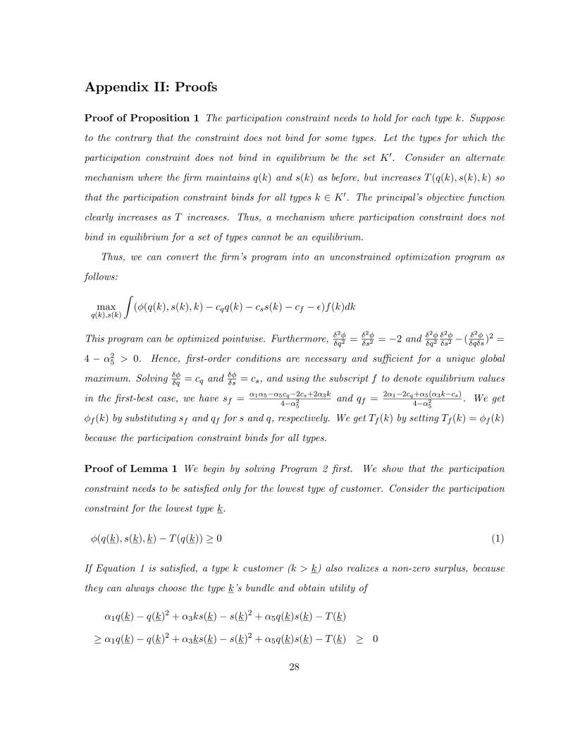
Appendix II: Proofs

Proof of Proposition 1 The participation constraint needs to hold for each type k. Suppose

to the contrary that the constraint does not bind for some types. Let the types for which the

participation constraint does not bind in equilibrium be the set K 0. Consider an alternate

mechanism where the firm maintains q(k) and s(k) as before, but increases T (q(k), s(k), k) so

that the participation constraint binds for all types k ∈ K 0. The principal’s objective function

clearly increases as T increases. Thus, a mechanism where participation constraint does not

bind in equilibrium for a set of types cannot be an equilibrium.

Thus, we can convert the firm’s program into an unconstrained optimization program as

follows:

maxq(k),s(k)

Z(φ(q(k), s(k), k)− cqq(k)− css(k)− cf − ²)f(k)dk

This program can be optimized pointwise. Furthermore, δ2φδq2

= δ2φδs2

= −2 and δ2φδq2

δ2φδs2−( δ2φδqδs)

2 =

4 − α25 > 0. Hence, first-order conditions are necessary and sufficient for a unique global

maximum. Solving δφδq = cq and

δφδs = cs, and using the subscript f to denote equilibrium values

in the first-best case, we have sf =α1α5−α5cq−2cs+2α3k

4−α25and qf =

2α1−2cq+α5(α3k−cs)4−α25

. We get

φf (k) by substituting sf and qf for s and q, respectively. We get Tf (k) by setting Tf (k) = φf (k)

because the participation constraint binds for all types.

Proof of Lemma 1 We begin by solving Program 2 first. We show that the participation

constraint needs to be satisfied only for the lowest type of customer. Consider the participation

constraint for the lowest type k.

φ(q(k), s(k), k)− T (q(k)) ≥ 0 (1)

If Equation 1 is satisfied, a type k customer (k > k) also realizes a non-zero surplus, because

they can always choose the type k’s bundle and obtain utility of

α1q(k)− q(k)2 + α3ks(k)− s(k)2 + α5q(k)s(k)− T (k)

≥ α1q(k)− q(k)2 + α3ks(k)− s(k)2 + α5q(k)s(k)− T (k) ≥ 0

28

Hence, if the participation constraint is satisfied for the lowest type, it is automatically

satisfied for all other types.

Observe that d2φds2

= −2. Hence, setting dφds = 0, we get s =

α3k+α5q2 . Substituting into φ, we

get

φ(q(k), k) =α23k

2 + 2α3α5kq(k) + q(k)(4α1 − (4− α25)q(k))

4(2)

The incentive compatibility constraints,

φ(q(k), s(k), k)− T (q(k)) ≥ φ(q(k̃), s̃, k)− T (q(k̃)), ∀k, k̃, s̃

become

φ(q(k), k)− T (q(k)) ≥ φ(q(k̃), k)− T (q(k̃)), ∀k, k̃

We can replace the incentive compatibility constraints with the following first-order condi-

tion.

dφ

dq− dTdq= 0 (3)

It remains to be verified that the second-order conditions are satisfied locally and globally and

we shall do so later.

To derive the optimal q(k) and s(k), we write the utility of customer type k as ι(k). From

the incentive compatibility constraint,

ι(k) ≡ φ(q(k), s(k), k)− T (q(k)) = maxk̃

φ(q(k̃), s(k̃), k)− T (q(k̃))

From the envelope theorem, dιdk =διδk since

διδq =

διδs = 0. Thus,

dι

dk= α3s(k) (4)

Integrating Equation 4, we can express the utility of type k customers as

ι(k) =

Z k

kα3s(k̃)dk̃ + ι(k) =

Z k

kα3s(k̃)dk̃

29

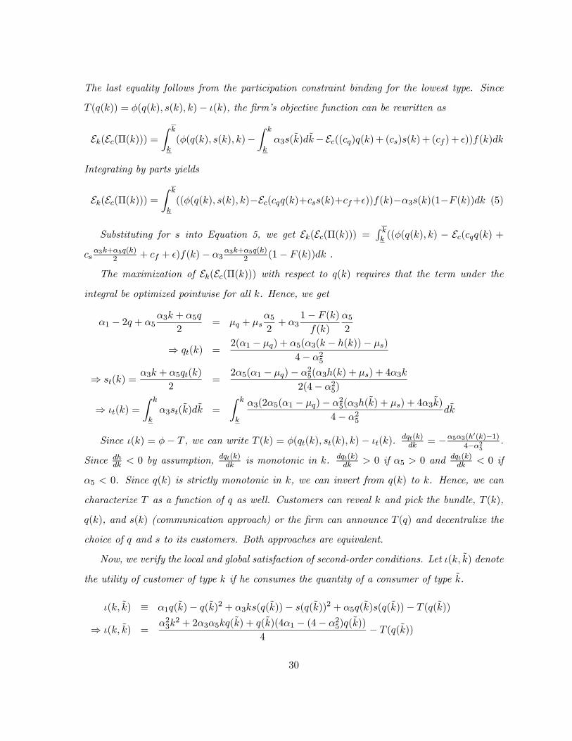
The last equality follows from the participation constraint binding for the lowest type. Since

T (q(k)) = φ(q(k), s(k), k)− ι(k), the firm’s objective function can be rewritten as

Ek(Ec(Π(k))) =Z k

k(φ(q(k), s(k), k)−

Z k

kα3s(k̃)dk̃− Ec((cq)q(k)+ (cs)s(k)+ (cf )+ ²))f(k)dk

Integrating by parts yields

Ek(Ec(Π(k))) =Z k

k((φ(q(k), s(k), k)−Ec(cqq(k)+css(k)+cf+²))f(k)−α3s(k)(1−F (k))dk (5)

Substituting for s into Equation 5, we get Ek(Ec(Π(k))) =R kk ((φ(q(k), k) − Ec(cqq(k) +

csα3k+α5q(k)

2 + cf + ²)f(k)− α3α3k+α5q(k)

2 (1− F (k))dk .The maximization of Ek(Ec(Π(k))) with respect to q(k) requires that the term under the

integral be optimized pointwise for all k. Hence, we get

α1 − 2q + α5α3k + α5q

2= µq + µs

α52+ α3

1− F (k)f(k)

α52

⇒ qt(k) =2(α1 − µq) + α5(α3(k − h(k))− µs)

4− α25

⇒ st(k) =α3k + α5qt(k)

2=

2α5(α1 − µq)− α25(α3h(k) + µs) + 4α3k

2(4− α25)

⇒ ιt(k) =

Z k

kα3st(k̃)dk̃ =

Z k

k

α3(2α5(α1 − µq)− α25(α3h(k̃) + µs) + 4α3k̃)

4− α25dk̃

Since ι(k) = φ− T , we can write T (k) = φ(qt(k), st(k), k)− ιt(k).dqt(k)dk = −α5α3(h0(k)−1)

4−α25.

Since dhdk < 0 by assumption, dqt(k)dk is monotonic in k. dqt(k)

dk > 0 if α5 > 0 and dqt(k)dk < 0 if

α5 < 0. Since q(k) is strictly monotonic in k, we can invert from q(k) to k. Hence, we can

characterize T as a function of q as well. Customers can reveal k and pick the bundle, T (k),

q(k), and s(k) (communication approach) or the firm can announce T (q) and decentralize the

choice of q and s to its customers. Both approaches are equivalent.

Now, we verify the local and global satisfaction of second-order conditions. Let ι(k, k̃) denote

the utility of customer of type k if he consumes the quantity of a consumer of type k̃.

ι(k, k̃) ≡ α1q(k̃)− q(k̃)2 + α3ks(q(k̃))− s(q(k̃))2 + α5q(k̃)s(q(k̃))− T (q(k̃))

⇒ ι(k, k̃) =α23k

2 + 2α3α5kq(k̃) + q(k̃)(4α1 − (4− α25)q(k̃))

4− T (q(k̃))

30

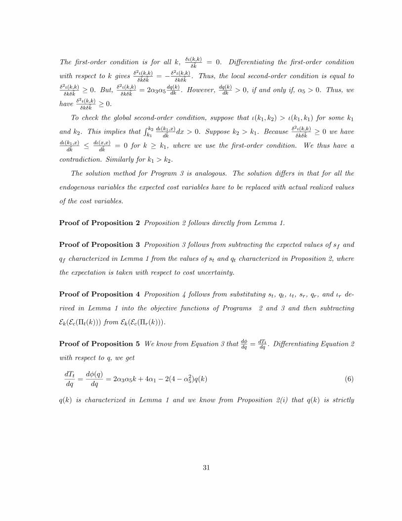
The first-order condition is for all k, δι(k,k)

δk̃= 0. Differentiating the first-order condition

with respect to k gives δ2ι(k,k)

δk̃δk̃= −δ2ι(k,k)

δkδk̃. Thus, the local second-order condition is equal to

δ2ι(k,k)

δkδk̃≥ 0. But, δ2ι(k,k)

δkδk̃= 2α3α5

dq(k)dk . However,

dq(k)dk > 0, if and only if, α5 > 0. Thus, we

have δ2ι(k,k)

δkδk̃≥ 0.

To check the global second-order condition, suppose that ι(k1, k2) > ι(k1, k1) for some k1

and k2. This implies thatR k2k1

dι(k1,x)

dk̃dx > 0. Suppose k2 > k1. Because

δ2ι(k,k)

δkδk̃≥ 0 we have

dι(k1,x)

dk̃≤ dι(x,x)

dk̃= 0 for k ≥ k1, where we use the first-order condition. We thus have a

contradiction. Similarly for k1 > k2.

The solution method for Program 3 is analogous. The solution differs in that for all the

endogenous variables the expected cost variables have to be replaced with actual realized values

of the cost variables.

Proof of Proposition 2 Proposition 2 follows directly from Lemma 1.

Proof of Proposition 3 Proposition 3 follows from subtracting the expected values of sf and

qf characterized in Lemma 1 from the values of st and qt characterized in Proposition 2, where

the expectation is taken with respect to cost uncertainty.

Proof of Proposition 4 Proposition 4 follows from substituting st, qt, ιt, sr, qr, and ιr de-

rived in Lemma 1 into the objective functions of Programs 2 and 3 and then subtracting

Ek(Ec(Πt(k))) from Ek(Ec(Πr(k))).

Proof of Proposition 5 We know from Equation 3 that dφdq =dTtdq . Differentiating Equation 2

with respect to q, we get

dTtdq

=dφ(q)

dq= 2α3α5k + 4α1 − 2(4− α25)q(k) (6)

q(k) is characterized in Lemma 1 and we know from Proposition 2(i) that q(k) is strictly

31

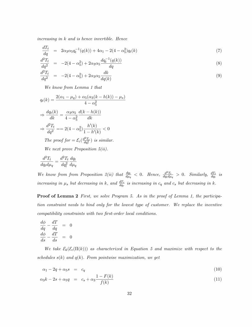
increasing in k and is hence invertible. Hence

dTtdq

= 2α3α5q−1t (q(k)) + 4α1 − 2(4− α25)qt(k) (7)

d2Ttdq2

= −2(4− α25) + 2α3α5dq−1t (q(k))

dq(8)

d2Ttdq2

= −2(4− α25) + 2α3α5dk

dq(k)(9)

We know from Lemma 1 that

qt(k) =2(α1 − µq) + α5(α3(k − h(k))− µs)

4− α25

⇒ dqt(k)

dk=

α3α54− α25

d(k − h(k))dk

⇒ d2Ttdq2

== 2(4− α25)h0(k)

1− h0(k) < 0

The proof for = Ec(d2Trdq2r) is similar.

We next prove Proposition 5(ii).

d2Ttdqtdµq

=d2Ttdq2t

dqtdµq

We know from from Proposition 2(ii) that dqtdµq

< 0. Hence, d2Ttdqtdµq

> 0. Similarly, dTtdqt

is

increasing in µs but decreasing in k, and dTrdqr

is increasing in cq and cs but decreasing in k.

Proof of Lemma 2 First, we solve Program 5. As in the proof of Lemma 1, the participa-

tion constraint needs to bind only for the lowest type of customer. We replace the incentive

compatibility constraints with two first-order local conditions.

dφ

dq− dTdq

= 0

dφ

ds− dTds

= 0

We take Ek(Ec(Π(k))) as characterized in Equation 5 and maximize with respect to theschedules s(k) and q(k). From pointwise maximization, we get

α1 − 2q + α5s = cq (10)

α3k − 2s+ α5q = cs + α31− F (k)f(k)

(11)

32

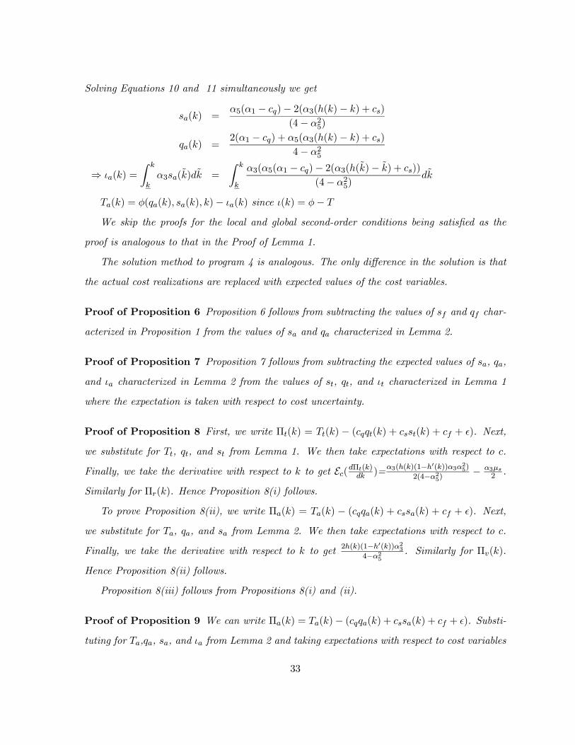
Solving Equations 10 and 11 simultaneously we get

sa(k) =α5(α1 − cq)− 2(α3(h(k)− k) + cs)

(4− α25)

qa(k) =2(α1 − cq) + α5(α3(h(k)− k) + cs)

4− α25

⇒ ιa(k) =

Z k

kα3sa(k̃)dk̃ =

Z k

k

α3(α5(α1 − cq)− 2(α3(h(k̃)− k̃) + cs))(4− α25)

dk̃

Ta(k) = φ(qa(k), sa(k), k)− ιa(k) since ι(k) = φ− TWe skip the proofs for the local and global second-order conditions being satisfied as the

proof is analogous to that in the Proof of Lemma 1.

The solution method to program 4 is analogous. The only difference in the solution is that

the actual cost realizations are replaced with expected values of the cost variables.

Proof of Proposition 6 Proposition 6 follows from subtracting the values of sf and qf char-

acterized in Proposition 1 from the values of sa and qa characterized in Lemma 2.

Proof of Proposition 7 Proposition 7 follows from subtracting the expected values of sa, qa,

and ιa characterized in Lemma 2 from the values of st, qt, and ιt characterized in Lemma 1

where the expectation is taken with respect to cost uncertainty.

Proof of Proposition 8 First, we write Πt(k) = Tt(k) − (cqqt(k) + csst(k) + cf + ²). Next,we substitute for Tt, qt, and st from Lemma 1. We then take expectations with respect to c.

Finally, we take the derivative with respect to k to get Ec(dΠt(k)dk )=α3(h(k)(1−h0(k))α3α25)2(4−α25)

− α3µs2 .

Similarly for Πr(k). Hence Proposition 8(i) follows.

To prove Proposition 8(ii), we write Πa(k) = Ta(k) − (cqqa(k) + cssa(k) + cf + ²). Next,we substitute for Ta, qa, and sa from Lemma 2. We then take expectations with respect to c.

Finally, we take the derivative with respect to k to get 2h(k)(1−h0(k))α234−α25

. Similarly for Πv(k).

Hence Proposition 8(ii) follows.

Proposition 8(iii) follows from Propositions 8(i) and (ii).

Proof of Proposition 9 We can write Πa(k) = Ta(k)− (cqqa(k) + cssa(k) + cf + ²). Substi-tuting for Ta,qa, sa, and ιa from Lemma 2 and taking expectations with respect to cost variables

33

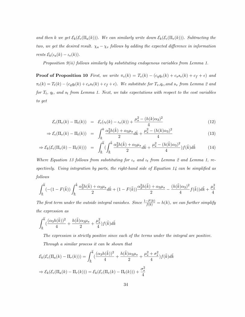
and then k we get Ek(Ec(Πa(k))). We can similarly write down Ek(Ec(Πv(k))). Subtracting thetwo, we get the desired result. χa−χv follows by adding the expected difference in information

rents Ek(ιa(k)− ιv(k)).

Proposition 9(ii) follows similarly by substituting endogenous variables from Lemma 1.

Proof of Proposition 10 First, we write πv(k) = Tv(k) − (cqqv(k) + cssv(k) + cf + ²) andπt(k) = Tt(k)− (cqqt(k) + csst(k) + cf + ²). We substitute for Tv,qv,and sv from Lemma 2 and

for Tt, qt, and st from Lemma 1. Next, we take expectations with respect to the cost variables

to get

Ec(Πv(k)−Πt(k)) = Ec(ιt(k)− ιv(k)) +µ2s − (h(k)α3)2

4(12)

⇒ Ec(Πv(k)−Πt(k)) =

Z k

k

α23h(k̂) + α3µs2

dk̂ +µ2s − (h(k)α3)2

4(13)

⇒ Ek(Ec(Πv(k)−Πt(k))) =

Z k

k(

Z k̃

k

α23h(k̂) + α3µs2

dk̂ +µ2s − (h(k̃)α3)2

4)f(k̃)dk̃ (14)

Where Equation 13 follows from substituting for ιv and ιt from Lemma 2 and Lemma 1, re-

spectively. Using integration by parts, the right-hand side of Equation 14 can be simplified as

followsZ k

k(−(1− F (k̃))

Z k̃

k

α23h(k̂) + α3µs2

dk̂ + (1− F (k̃))α23h(k̃) + α3µs

2− (h(k̃)α3)

2

4f(k̃))dk̃ +

µ2s4

The first term under the outside integral vanishes. Since 1−F (k)f(k) = h(k), we can further simplify

the expression asZ k

k((α3h(k̃))

2

4+h(k̃)α3µs

2+µ2s4)f(k̃)dk̃

The expression is strictly positive since each of the terms under the integral are positive.

Through a similar process it can be shown that

Ek(Ec(Πa(k)−Πr(k))) =Z k

k((α3h(k̃))

2

4+h(k̃)α3µs

2+µ2s + σ2s4

)f(k̃)dk̃

⇒ Ek(Ec(Πa(k)−Πr(k))) = Ek(Ec(Πv(k)−Πt(k))) + σ2s4

34

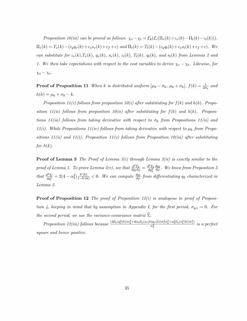
Proposition 10(iii) can be proved as follows. χv−χt = Ek(Ec(Πv(k)+ ιv(k)−Πt(k)− ιt(k))).Πv(k) = Tv(k)−(cqqv(k)+cssv(k)+cf +²) and Πt(k) = Tt(k)−(cqqt(k)+csst(k)+cf +²). Wecan substitute for ιv(k),Tv(k), qv(k), sv(k), ιt(k), Tt(k), qt(k), and st(k) from Lemmas 2 and

1. We then take expectations with respect to the cost variables to derive χv − χt. Likewise, for

χa − χr.

Proof of Proposition 11 When k is distributed uniform [µk − σk, µk + σk], f(k) = 12σk

and

h(k) = µk + σk − k.Proposition 11(i) follows from proposition 10(i) after substituting for f(k) and h(k). Propo-

sition 11(ii) follows from proposition 10(ii) after substituting for f(k) and h(k). Proposi-

tions 11(iii) follows from taking derivative with respect to σk from Propositions 11(ii) and

11(i). While Propositions 11(iv) follows from taking derivative with respect to µk from Propo-

sitions 11(ii) and 11(i), Proposition 11(v) follows from Proposition 10(iii) after substituting

for h(k).

Proof of Lemma 3 The Proof of Lemma 3(i) through Lemma 3(ii) is exactly similar to the

proof of Lemma 1. To prove Lemma 3(v), see that d2T2dq2dϕ

= d2T2dq22

dq2dϕ . We know from Proposition 5

that d2Ttdq2t

= 2(4− α25)h0(k)1−h0(k) < 0. We can compute

dq2dϕ from differentiating q2 characterized in

Lemma 3.

Proof of Proposition 12 The proof of Proposition 12(i) is analogous to proof of Proposi-

tion 4, keeping in mind that by assumption in Appendix I, for the first period, σq,s = 0. For

the second period, we use the variance-covariance matrix eΣ.Proposition 12(iii) follows because

(4Ek(q21(k))σ4q+4α5Ek(s1(k)q1(k))σ2sσ2q+α25Ek(s21(k))σ4s)σ2η

is a perfect

square and hence positive.

35

References

Adams, W. J. and J. L. Yellen, (1976) “Commodity Bundling and the Burden of Monopoly”

Quarterly Journal of Economics 90 (August) 475-498.

Banker, R. and J. Hughes, (1994) “ Product Costing and Pricing” The Accounting Review 69

July 1994.

Banker and Potter (1993) “Economic Implications of Single Cost Driver Systems" Journal of

Management Accounting Research Fall 1993 pp 15-32.

Baron and Myerson (1982) “Regulating a Monopolist with Unknown Costs" Econometrica 50:

pp 911-930.

Brem L. and V.G. Narayanan (2000) “Owens and Minor(A) and (B)” Harvard Business School

Cases.

Cooper R. and R. Kaplan (1988) “Measure Costs Right: Make the Right Decisions,” Harvard

Business Review (September-October) pp. 97-98.

Cooper R. and R. Kaplan (1991) “Profit Priorities from Activity-Based Costing,”Harvard

Business Review (May—June) pp. 130-135.

Foster G. and M. Gupta (1998) “The Customer Profitability Implications of Customer Satis-

faction,” Washington University Working Paper.

Foster G., M. Gupta, and L. Sjoblom (1995) “Customer Profitability Analysis,” Journal of

Cost Management.

Kirby, A. J., S. Reichelstein, P.K. Sen, Pradyot, and T.K. Paik,(1991) “Participation, Slack,

and Budget-Based Performance Evaluation” Journal of Accounting Research Spring pp.109:138

Larsen, J, and V.G. Narayanan (2000), “Menu Based Pricing" Harvard Business School Work-

ing paper.

McAfee, R. P., J. McMillan, and M.D. Whinston (1989) “ Multi-product Monopoly, Commod-

ity Bundling, and Correlation of Values” Quarterly Journal of Economics 114 (May):371-

384.

36

Melumad, N, D. Mookherjee, and S. Reichelstein, (1992) “A Theory of Responsibility Centers

” Journal of Accounting and Economics Dec pp. 445-485.

Narayanan V. G. and R. Sarkar (2000)“The Impact of Activity-Based Costing on Managerial

Decisions at Insteel Industries- A Field Study,” Forthcoming Journal of Economics and

Management Strategy.

Niraj R., M. Gupta and C. Narasimhan (1999) “Customer Profitability in a Supply Chain”

University of Washington working paper.

Schmalensee, R.L. (1984) “Gaussian Demand and Commodity Bundling” Journal of Business

57(January):S211-S230.

Stigler, G.J. (1968) “A Note on Block Booking” In G.J. Stigler, The Organization of Industry

Homewood, Ill.: Richard D. Irwin.

Stole, L. (1995) “Nonlinear Pricing and Oligopoly” Journal of Economics and Management

Strategy Volume 4, Number 4, Winter, pp. 529-562.

Tirole J. (1988) “ The Theory of Industrial Organization” The MIT Press Cambridge, Massa-

chusetts

37