Active wide band antenna for under water tomography (1 GHz)1

C.Conessa and A.Joisel

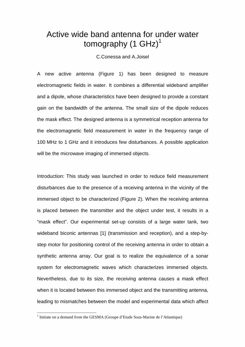
A new active antenna (Figure 1) has been designed to measure

electromagnetic fields in water. It combines a differential wideband amplifier

and a dipole, whose characteristics have been designed to provide a constant

gain on the bandwidth of the antenna. The small size of the dipole reduces

the mask effect. The designed antenna is a symmetrical reception antenna for

the electromagnetic field measurement in water in the frequency range of

100 MHz to 1 GHz and it introduces few disturbances. A possible application

will be the microwave imaging of immersed objects.

Introduction: This study was launched in order to reduce field measurement

disturbances due to the presence of a receiving antenna in the vicinity of the

immersed object to be characterized (Figure 2). When the receiving antenna

is placed between the transmitter and the object under test, it results in a

“mask effect”. Our experimental set-up consists of a large water tank, two

wideband biconic antennas [1] (transmission and reception), and a step-by-

step motor for positioning control of the receiving antenna in order to obtain a

synthetic antenna array. Our goal is to realize the equivalence of a sonar

system for electromagnetic waves which characterizes immersed objects.

Nevertheless, due to its size, the receiving antenna causes a mask effect

when it is located between this immersed object and the transmitting antenna,

leading to mismatches between the model and experimental data which affect

1 Initiate on a demand from the GESMA (Groupe d’Etude Sous-Marine de l’Atlantique)

the images reconstructions. In order to reduce these mismatches, a new

antenna which introduces a smaller mask effect has been developed. A

similar approach has been used for astronomical studies [2]. As uncommonly

under water near-field measurements are not well studied, a first investigation

of such systems has been done.

Antenna development: Using a short dipole instead of a thick wide band

conventional antenna allows the mask effect to be reduced drastically. This

dipole can be connected to a differential amplifier which is used as a wide-

band matching network and ideal balun. A short antenna ( l << λ ) presents

two advantages: i) its omnidirectional pattern is quite independent of the

frequency and ii) this antenna works like a field measurement device over a

wide frequency band, while the drawbacks are i) the impedance of the dipole

varies greatly with the frequency and ii) it has poor sensitivity specially for the

low frequencies. Hence the dipole is connected to a high input impedance

differential amplifier which acts as a perfect wide band balun.

Also, we calculated the length of the dipole to have the resonance frequency

near the end of the amplifier‘s bandwidth at 900 MHz. AD8351, a CMS

integrated circuit is selected for the amplification as it has a differential input

and a stable gain between 1 to 1000 MHz. Moreover, its small size (2.1 cm)

means that less disturbance is introduced to the system.

For practical reasons, a short transmission line is needed to connect the

dipole to the amplifier input. The impedance of this line is 73 Ω, matched to

the dipole only at the resonance frequency. As the dipole and the amplifier

impedances are not matched to the transmission line over the operating

frequency band, it is necessary to adjust the length of this line to minimize

mismatch effects. In order to optimize the length of the line, the equivalent

circuit of the “antenna-line-amplifier” system (Figure 3) has been simulated

using Matlab. The impedance Za of the antenna is given by Johnson and Jasik

model [3].

Za = R( )kl – j

120

ln

la – 1 cot kl – X(kl) ,

Where :

Za is the impedance in ohms of a dipole which is a cylinder with a length of

l = l0/2 and a radius of a.

kl = 2 π (l/λ) (in radians) is an electric length and the functions R(kl) and X(kl)

given by [3]. The amplifier input impedance are given by data sheet of the

selected integrated circuit [4]. The amplifier input is taken to be a 5 kΩ

resistance in parallel with a 0.8 pF capacitor.

The transfer function of the system between the dipole connection and the

device output is :

T (jω) = Ze

Ze + Za,L

Re(Za,L)Re(Za)

Where Ze is the input impedance of the amplifier given by:

Ze = Re

1 + j Re Ce ω

And Za, L is the impedance measured at a given position L from the dipole

trough the line between the amplifier input and the antenna and it is given by :

Za, L = ZdZa + j Zd tan(β L) Zd + j Za tan(β L)

Where Zd is the characteristic impedance of the line (73 Ω),

β = 2πλ

is the propagation constant and L is the length of the line.

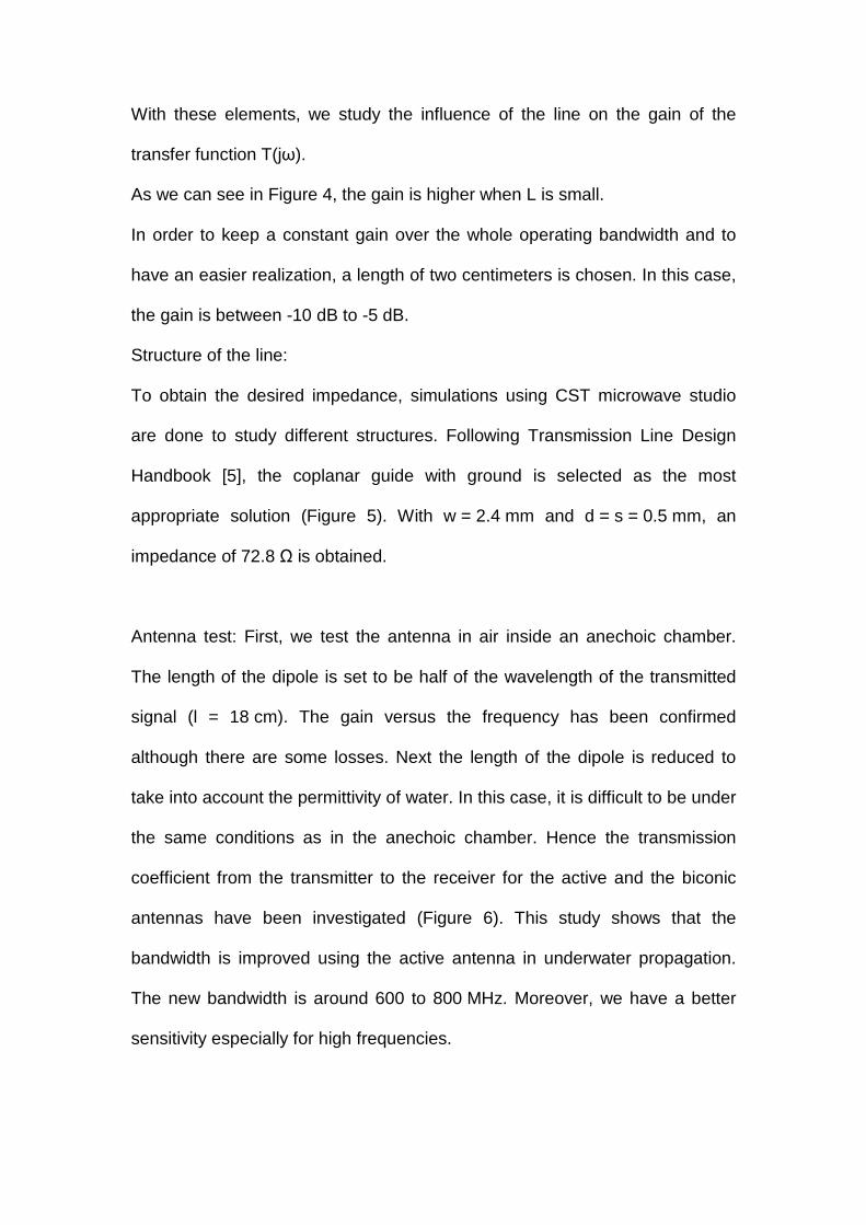
With these elements, we study the influence of the line on the gain of the

transfer function T(jω).

As we can see in Figure 4, the gain is higher when L is small.

In order to keep a constant gain over the whole operating bandwidth and to

have an easier realization, a length of two centimeters is chosen. In this case,

the gain is between -10 dB to -5 dB.

Structure of the line:

To obtain the desired impedance, simulations using CST microwave studio

are done to study different structures. Following Transmission Line Design

Handbook [5], the coplanar guide with ground is selected as the most

appropriate solution (Figure 5). With w = 2.4 mm and d = s = 0.5 mm, an

impedance of 72.8 Ω is obtained.

Antenna test: First, we test the antenna in air inside an anechoic chamber.

The length of the dipole is set to be half of the wavelength of the transmitted

signal (l = 18 cm). The gain versus the frequency has been confirmed

although there are some losses. Next the length of the dipole is reduced to

take into account the permittivity of water. In this case, it is difficult to be under

the same conditions as in the anechoic chamber. Hence the transmission

coefficient from the transmitter to the receiver for the active and the biconic

antennas have been investigated (Figure 6). This study shows that the

bandwidth is improved using the active antenna in underwater propagation.

The new bandwidth is around 600 to 800 MHz. Moreover, we have a better

sensitivity especially for high frequencies.

Conclusion: This study opens the path to new developments. The new active

probe is smaller than the biconic system, hence resulting in less disturbance.

Its gain is also higher than the former system. Simple, cheap and easy to

build, becomes possible to build an antenna array for immersed object

imaging with low disturbance. The sensitivity is also better especially for high

frequencies. As a consequence the spatial resolution of tomographic systems

using such probes can be improved. Before realizing a probe array using this

principle, the prototype could be improved, by optimizing other parameters

such as dipole and differential line lengths.

References 1 Duchêne, B. and Joisel, A. and Lambert, M., “Nonlinear inversions of immersed objects from laboratory-controlled data, Inverse Problems, Special section on the Electromagnetic Characterization of Buried Obstacles”, D. Lesselier and W. C. Chew Eds., 2004, 20, 6, S81-S98, December 2 Ardouin, D.; Bellétoile, A.; Charrier, D.; Dallier, R.; Denis, L.; Eschstruth, P.; Gousset, T.; Haddad, F.; Lamblin, J.; Lautridou, P.; Lecacheux, A.; Monnier-Ragaigne, D.; Rahmani, A.; Ravel, O., ”Radio-detection signature of high-energy cosmic rays by the CODALEMA experiment”, 2005 december, Nuclear Instruments and Methods in Physics Research Section A, Volume 555, Issue 1-2, p. 148-163, 3 R. JOHNSON, H. JASIK, "Antenna Engineering Handbook, second edition", 1993, Mc Graw Hill Publication 4 ANALOG DEVICES, "Low Distortion, Differential RF/IF Amplifier, AD8351", Rev. B, 2003. 5 BRAIN C. WADELL, "Transmission Line Design Handbook", 1991 June, Artech House Publishers

Figure captions:

Figure 1 Active antenna photos

Figure 2 Experimental setup

Figure 3 Equivalent circuit for the system “antenna-line-amplifier”

Figure 4 Influence’s study of the line’s length on the gain versus frequency

Figure 5 Structure of the differential line

Figure 6 Transmission coefficients comparison between influence’s study of the line’s length on the gain versus frequency

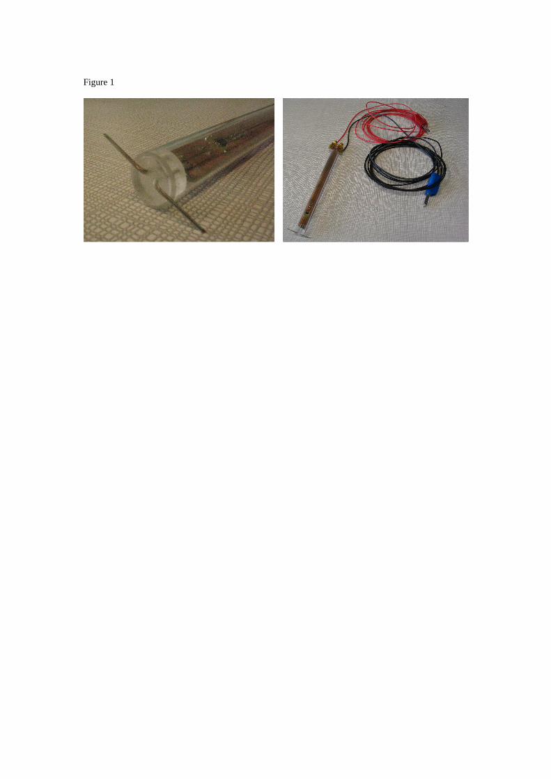
Figure 1

Figure 2

R T T = Transmitter R = Receiver

Water

Object

Figure 3

Za

Ll, Zc

Ze

ea

Figure 4

100 200 300 400 500 600 700 800 9000

0.01

0.02

0.03

0.04

0.05

0.06

0.07

0.08

0.09

0.1

Frequency (MHz)

Leng

th o

f the

line

(m)

-50

-40

-30

-20

-10

0

10

Gain (dB

)

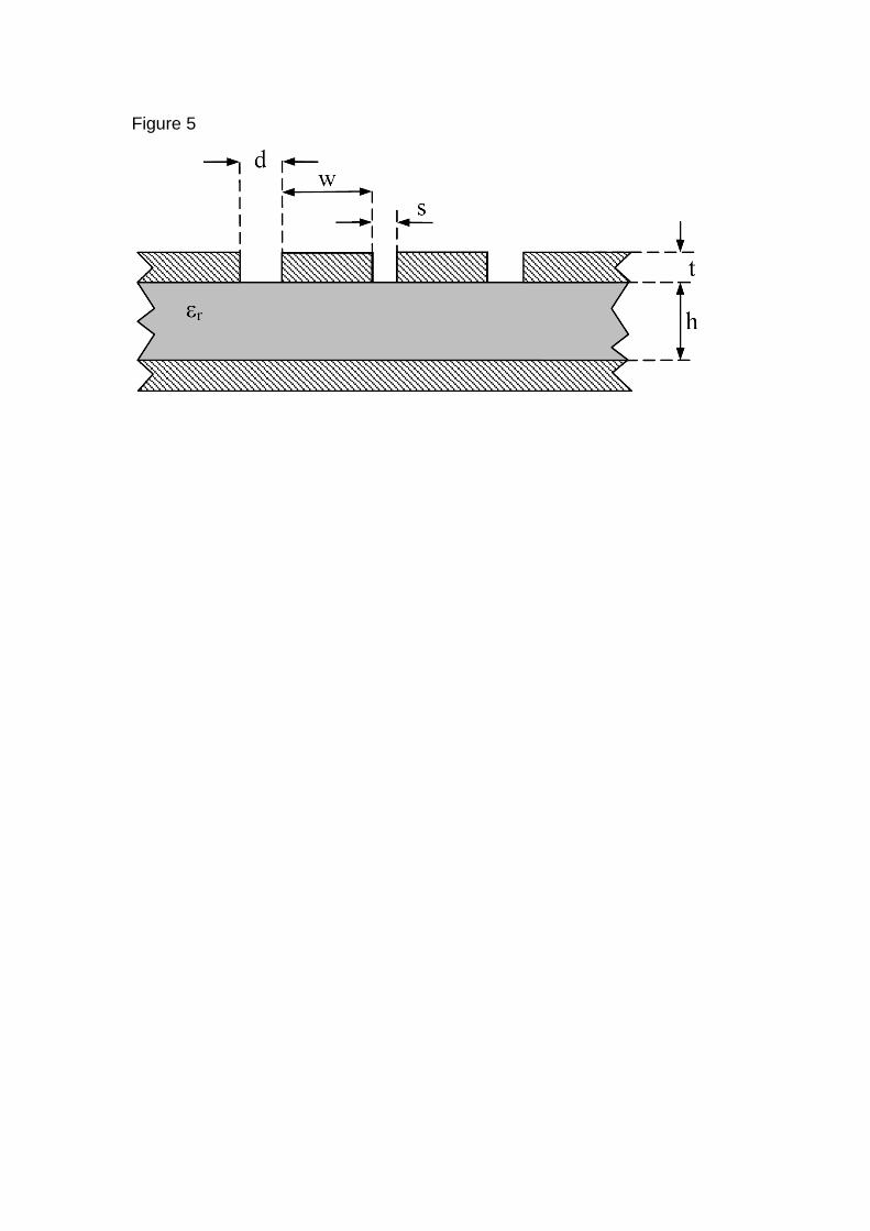
Figure 5

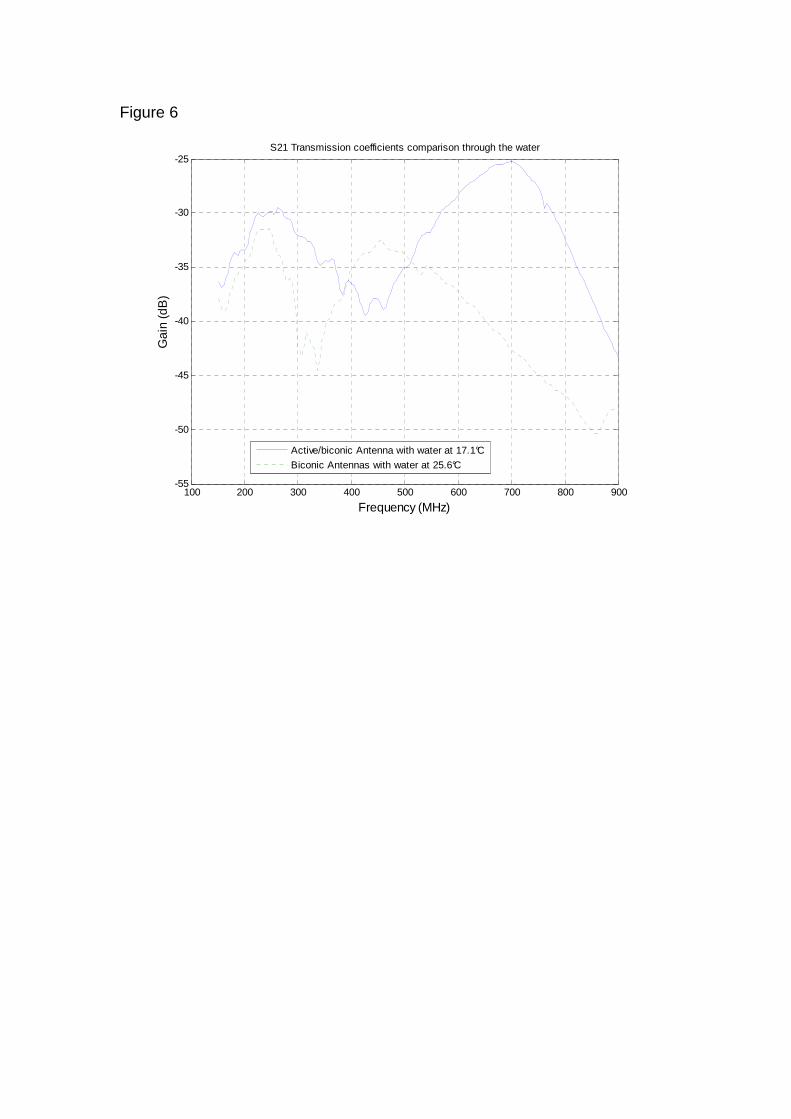
Figure 6

100 200 300 400 500 600 700 800 900-55

-50

-45

-40

-35

-30

-25

Frequency (MHz)

Gai

n (d

B)

S21 Transmission coefficients comparison through the water

Active/biconic Antenna with water at 17.1°C

Biconic Antennas with water at 25.6°C