Thesis Summary:

Active Visual SLAM with Explorationfor Autonomous Underwater Navigation

Ayoung Kim

1 Introduction

Autonomous underwater vehicles (AUVs) have played an important role in scientific research dueto their ability to collect data in underwater environments that are either inaccessible or too dan-gerous for humans to explore. Other than explorations, underwater structures such as dams, shiphulls, harbors and pipelines also need to be periodically inspected for assessment, maintenance andsecurity reasons. Autonomous vehicles have the potential for better coverage efficiency, improvedsurvey precision and overall reduced need for human intervention.

In comparison to terrestrial navigation, underwater navigation is challenging because the opac-ity of water to electromagnetic waves precludes the use of the global positioning system (GPS)and other high speed radio communication. Due to the lack of accurate position information fromGPS, traditional underwater navigation methods have been used to solve the navigation problemusing acoustic signals. Traditionally, navigation limitations can be overcome by using a simultane-ous localization and mapping (SLAM) algorithm to fuse sensor measurements derived from visionand/or sonar. Similar to human navigation, in which sight confirms our position when we recognizea previously visited scene, visual measurements significantly reduce the uncertainty when a site isrevisited and recognized (i.e., loop-closing). The advantage of visual SLAM arises from these loop-closure camera measurements, which add independent constraints to the pose-graph, and greatlyreduce position uncertainty as compared to pure odometry (dead reckoning).

Despite this major contribution in reducing uncertainty, visual measurements may not be uni-formly available in an underwater environment where the spatial feature distribution varies greatly.This indicates that successful measurements strongly depend upon two factors: (i) the saliency ofvisual features and (ii) their spatial distribution as seen by the robot. The first factor, saliency, isan image measurement that represents distinguishability of a visual feature. The second factor, theobserved spatial distribution, is mainly determined by the environment and egomotion of the robot(e.g., path and gaze). A similar interrelation has been proposed by [1] who found that changes intrajectory can result in better navigation. However, we should note that these two factors shouldbe considered simultaneously for better navigation results, especially for underwater images wherethe possibility of making a valid registration may not be as uniform as in the terrestrial environ-ment. Based upon this motivation, this thesis’s goal has been to develop a control scheme forbetter navigation by providing trajectory perturbations to improve pose observability under theconsideration of a visual saliency map.

2 Real-time Pose-graph Visual SLAM

The real-time pose-graph visual SLAM presented in this thesis is an extension of visually augmentednavigation (VAN) [2] to include geometric model selection for robust image registration, mainlyfocusing on pose-graph visual SLAM.

1

Camera footprint

Sonar footprint

HAUV

(a) Periscope mode

Thrusters

Camera

LED Light

DVLDIDSON Sonar

(b) Underwater mode

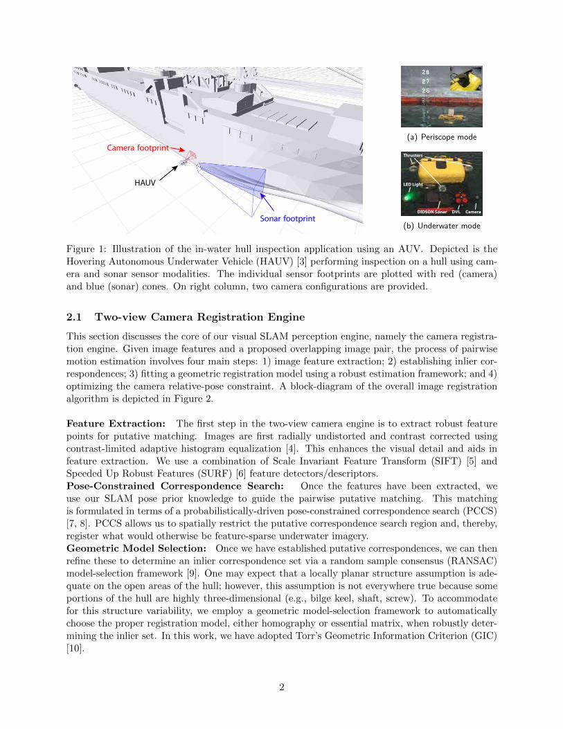
Figure 1: Illustration of the in-water hull inspection application using an AUV. Depicted is theHovering Autonomous Underwater Vehicle (HAUV) [3] performing inspection on a hull using cam-era and sonar sensor modalities. The individual sensor footprints are plotted with red (camera)and blue (sonar) cones. On right column, two camera configurations are provided.

2.1 Two-view Camera Registration Engine

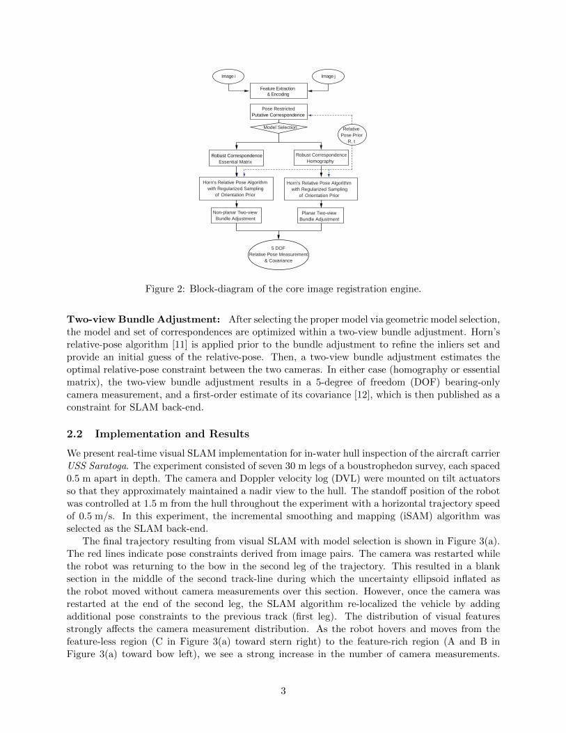
This section discusses the core of our visual SLAM perception engine, namely the camera registra-tion engine. Given image features and a proposed overlapping image pair, the process of pairwisemotion estimation involves four main steps: 1) image feature extraction; 2) establishing inlier cor-respondences; 3) fitting a geometric registration model using a robust estimation framework; and 4)optimizing the camera relative-pose constraint. A block-diagram of the overall image registrationalgorithm is depicted in Figure 2.

Feature Extraction: The first step in the two-view camera engine is to extract robust featurepoints for putative matching. Images are first radially undistorted and contrast corrected usingcontrast-limited adaptive histogram equalization [4]. This enhances the visual detail and aids infeature extraction. We use a combination of Scale Invariant Feature Transform (SIFT) [5] andSpeeded Up Robust Features (SURF) [6] feature detectors/descriptors.Pose-Constrained Correspondence Search: Once the features have been extracted, weuse our SLAM pose prior knowledge to guide the pairwise putative matching. This matchingis formulated in terms of a probabilistically-driven pose-constrained correspondence search (PCCS)[7, 8]. PCCS allows us to spatially restrict the putative correspondence search region and, thereby,register what would otherwise be feature-sparse underwater imagery.Geometric Model Selection: Once we have established putative correspondences, we can thenrefine these to determine an inlier correspondence set via a random sample consensus (RANSAC)model-selection framework [9]. One may expect that a locally planar structure assumption is ade-quate on the open areas of the hull; however, this assumption is not everywhere true because someportions of the hull are highly three-dimensional (e.g., bilge keel, shaft, screw). To accommodatefor this structure variability, we employ a geometric model-selection framework to automaticallychoose the proper registration model, either homography or essential matrix, when robustly deter-mining the inlier set. In this work, we have adopted Torr’s Geometric Information Criterion (GIC)[10].

2

Pose Restricted

Feature Extraction & Encoding

Image i

Putative Correspondence

Horn's Relative Pose Algorithmwith Regularized Sampling

of Orientation Prior

Non-planar Two-viewBundle Adjustment

Horn's Relative Pose Algorithmwith Regularized Sampling

of Orientation Prior

Planar Two-view Bundle Adjustment

5 DOFRelative Pose Measurement

& Covariance

Model Selection

Robust CorrespondenceEssential Matrix

Robust CorrespondenceHomography

Image j

RelativePose Prior

R, t

Figure 2: Block-diagram of the core image registration engine.

Two-view Bundle Adjustment: After selecting the proper model via geometric model selection,the model and set of correspondences are optimized within a two-view bundle adjustment. Horn’srelative-pose algorithm [11] is applied prior to the bundle adjustment to refine the inliers set andprovide an initial guess of the relative-pose. Then, a two-view bundle adjustment estimates theoptimal relative-pose constraint between the two cameras. In either case (homography or essentialmatrix), the two-view bundle adjustment results in a 5-degree of freedom (DOF) bearing-onlycamera measurement, and a first-order estimate of its covariance [12], which is then published as aconstraint for SLAM back-end.

2.2 Implementation and Results

We present real-time visual SLAM implementation for in-water hull inspection of the aircraft carrierUSS Saratoga. The experiment consisted of seven 30 m legs of a boustrophedon survey, each spaced0.5 m apart in depth. The camera and Doppler velocity log (DVL) were mounted on tilt actuatorsso that they approximately maintained a nadir view to the hull. The standoff position of the robotwas controlled at 1.5 m from the hull throughout the experiment with a horizontal trajectory speedof 0.5 m/s. In this experiment, the incremental smoothing and mapping (iSAM) algorithm wasselected as the SLAM back-end.

The final trajectory resulting from visual SLAM with model selection is shown in Figure 3(a).The red lines indicate pose constraints derived from image pairs. The camera was restarted whilethe robot was returning to the bow in the second leg of the trajectory. This resulted in a blanksection in the middle of the second track-line during which the uncertainty ellipsoid inflated asthe robot moved without camera measurements over this section. However, once the camera wasrestarted at the end of the second leg, the SLAM algorithm re-localized the vehicle by addingadditional pose constraints to the previous track (first leg). The distribution of visual featuresstrongly affects the camera measurement distribution. As the robot hovers and moves from thefeature-less region (C in Figure 3(a) toward stern right) to the feature-rich region (A and B inFigure 3(a) toward bow left), we see a strong increase in the number of camera measurements.

3

510

1520

2530

352

4

Longitudinal [m]

Dep

th [m

]

A B

C

(a) SLAM result from the USS Saratoga (b) Texture mapped reconstruction

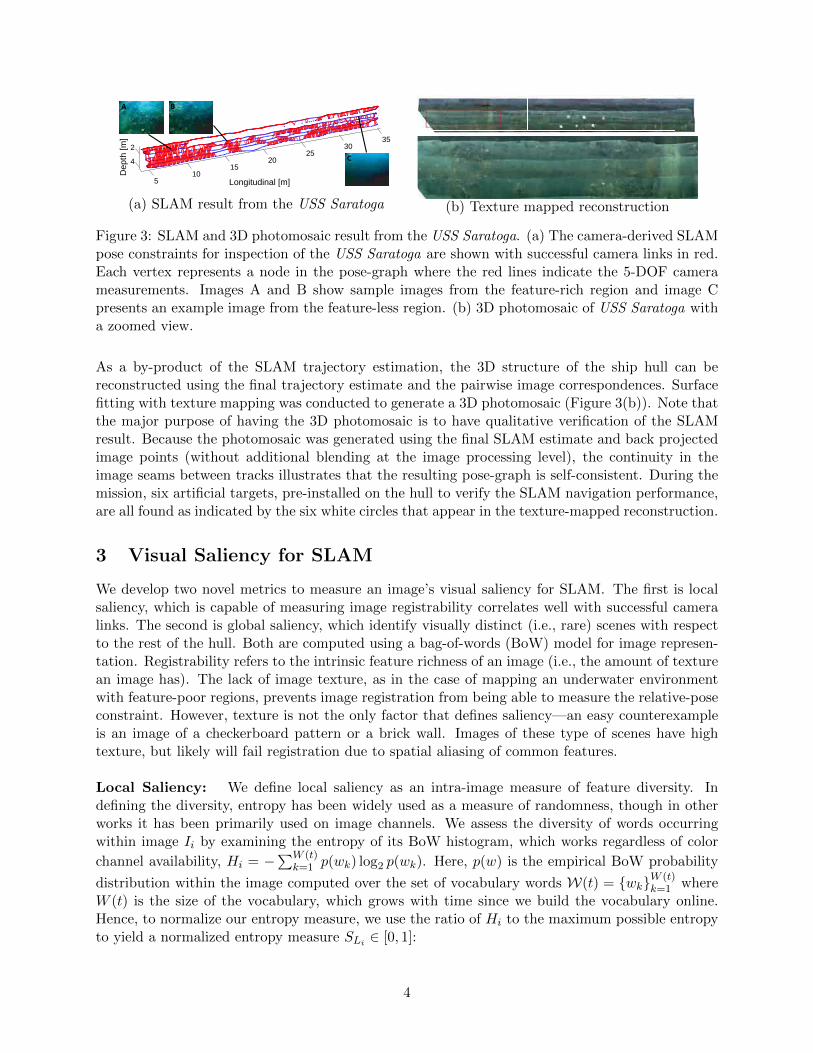
Figure 3: SLAM and 3D photomosaic result from the USS Saratoga. (a) The camera-derived SLAMpose constraints for inspection of the USS Saratoga are shown with successful camera links in red.Each vertex represents a node in the pose-graph where the red lines indicate the 5-DOF camerameasurements. Images A and B show sample images from the feature-rich region and image Cpresents an example image from the feature-less region. (b) 3D photomosaic of USS Saratoga witha zoomed view.

As a by-product of the SLAM trajectory estimation, the 3D structure of the ship hull can bereconstructed using the final trajectory estimate and the pairwise image correspondences. Surfacefitting with texture mapping was conducted to generate a 3D photomosaic (Figure 3(b)). Note thatthe major purpose of having the 3D photomosaic is to have qualitative verification of the SLAMresult. Because the photomosaic was generated using the final SLAM estimate and back projectedimage points (without additional blending at the image processing level), the continuity in theimage seams between tracks illustrates that the resulting pose-graph is self-consistent. During themission, six artificial targets, pre-installed on the hull to verify the SLAM navigation performance,are all found as indicated by the six white circles that appear in the texture-mapped reconstruction.

3 Visual Saliency for SLAM

We develop two novel metrics to measure an image’s visual saliency for SLAM. The first is localsaliency, which is capable of measuring image registrability correlates well with successful cameralinks. The second is global saliency, which identify visually distinct (i.e., rare) scenes with respectto the rest of the hull. Both are computed using a bag-of-words (BoW) model for image represen-tation. Registrability refers to the intrinsic feature richness of an image (i.e., the amount of texturean image has). The lack of image texture, as in the case of mapping an underwater environmentwith feature-poor regions, prevents image registration from being able to measure the relative-poseconstraint. However, texture is not the only factor that defines saliency—an easy counterexampleis an image of a checkerboard pattern or a brick wall. Images of these type of scenes have hightexture, but likely will fail registration due to spatial aliasing of common features.

Local Saliency: We define local saliency as an intra-image measure of feature diversity. Indefining the diversity, entropy has been widely used as a measure of randomness, though in otherworks it has been primarily used on image channels. We assess the diversity of words occurringwithin image Ii by examining the entropy of its BoW histogram, which works regardless of color

channel availability, Hi = −∑W (t)

k=1 p(wk) log2 p(wk). Here, p(w) is the empirical BoW probability

distribution within the image computed over the set of vocabulary words W(t) = {wk}W (t)k=1 where

W (t) is the size of the vocabulary, which grows with time since we build the vocabulary online.Hence, to normalize our entropy measure, we use the ratio of Hi to the maximum possible entropyto yield a normalized entropy measure SLi ∈ [0, 1]:

4

SLi =Hi

log2W (t). (1)

This entropy-derived measure captures the diversity of words (descriptors) appearing within animage.Global Saliency: We define global saliency as an inter-image measure of the uniqueness orrarity of features occurring within an image. To tackle this problem, we use inverse documentfrequency (idf) [13, 14, 15] to detect rare words and expect a high idf for words (descriptors) that

are rare in the dataset. Gi(t) =∑

k∈Wilog2

N(t)nwk

(t) . Here, Wi ⊂ W(t) represents the subset of

vocabulary words occurring within image Ii, nwk(t) is the current number of documents in the

database containing word wk, and N(t) is the current number of documents in the database. Toguarantee independent sample statistics used in our idf calculation, only spatially distinct (i.e.,non-overlapping) images are used to update nwk

(t) and N(t). Lastly, as was the case with our localsaliency measure, we normalize the rarity measure for image Ii to have a normalized global saliencyscore SGi ∈ [0, 1]:

SGi(t) =Gi(t)Gmax

, (2)

where the normalizer, Gmax, is the maximum summed idf score encountered thus far.

3.1 Saliency-informed Visual SLAM

Using our previously defined local saliency measure, we can improve the performance of visualSLAM in two ways:

1. We can sparsify the pose-graph by retaining only visually salient keyframes;

2. We can make link proposals within the graph more efficient and robust by combining visualsaliency with measures of geometric information gain.

In the first step, we can decide whether or not a keyframe should be added at all to the graphby evaluating its local saliency level—this allows us to cull visually homogeneous imagery, whichresults in a graph that is more sparse and visually informative. This improves the overall efficiencyof graph inference and eliminates nodes that would otherwise have low utility in underwater visualperception.

In the second step, we can improve the efficiency of link proposal by making it “salient-aware”.For efficient link proposal, [16] used expected information gain to prioritize which edges to add tothe graph—thereby retaining only informative links. However, when considering the case of visualperception, not all camera-derived measurements are equally obtainable. Pairwise registration oflow local saliency images will fail unless there is a strong prior to guide the putative correspondencesearch, whereas pairwise registration of highly salient image pairs often succeeds even with a weakor uninformative prior. Hence, when evaluating the expected information gain of proposed links,we should take into account their visual saliency, as this is an overall good indicator of whetheror not the expected information gain (i.e., image registration) is actually obtainable. By doing so,we can propose the addition of links that are not only geometrically informative, but also visuallyplausible.

5

A B C D E F G H

globally salient locally salient

(a) Sample images

0 5 10 15 20 25

−40

−35

−30

−25

−20

−15

−10

−5

0

5

Lateral [m]

Lo

ng

itu

din

al [m

]

(b) Camera constraints

0 5 10 15 20 25

−40

−35

−30

−25

−20

−15

−10

−5

0

5

Lateral [m]

Longitudin

al [m

]

A

E

B

H

F

D

CG

0

0.2

0.4

0.6

0.8

1

(c) Local saliency SL

0 5 10 15 20 25

−40

−35

−30

−25

−20

−15

−10

−5

0

5

Lateral [m]

Longitudin

al [m

]

A

E

B

H

F

D

CG

(d) Global saliency SG

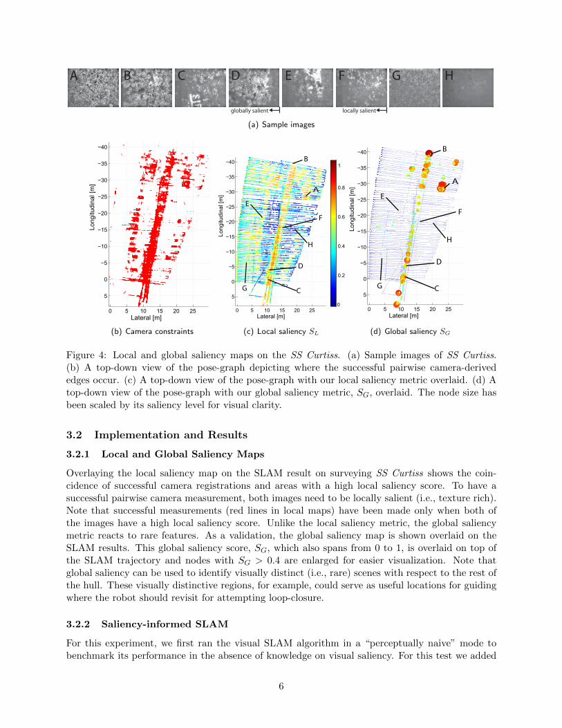
Figure 4: Local and global saliency maps on the SS Curtiss. (a) Sample images of SS Curtiss.(b) A top-down view of the pose-graph depicting where the successful pairwise camera-derivededges occur. (c) A top-down view of the pose-graph with our local saliency metric overlaid. (d) Atop-down view of the pose-graph with our global saliency metric, SG, overlaid. The node size hasbeen scaled by its saliency level for visual clarity.

3.2 Implementation and Results

3.2.1 Local and Global Saliency Maps

Overlaying the local saliency map on the SLAM result on surveying SS Curtiss shows the coin-cidence of successful camera registrations and areas with a high local saliency score. To have asuccessful pairwise camera measurement, both images need to be locally salient (i.e., texture rich).Note that successful measurements (red lines in local maps) have been made only when both ofthe images have a high local saliency score. Unlike the local saliency metric, the global saliencymetric reacts to rare features. As a validation, the global saliency map is shown overlaid on theSLAM results. This global saliency score, SG, which also spans from 0 to 1, is overlaid on top ofthe SLAM trajectory and nodes with SG > 0.4 are enlarged for easier visualization. Note thatglobal saliency can be used to identify visually distinct (i.e., rare) scenes with respect to the rest ofthe hull. These visually distinctive regions, for example, could serve as useful locations for guidingwhere the robot should revisit for attempting loop-closure.

3.2.2 Saliency-informed SLAM

For this experiment, we first ran the visual SLAM algorithm in a “perceptually naive” mode tobenchmark its performance in the absence of knowledge on visual saliency. For this test we added

6

0

5

10

15

20

25

30

35

−40

−30

−20

−10

0

2

46

8

Longitudinal [m]Lateral [m]

De

pth

[m

]

SLAM DR

(a) Visual SLAM result with only salient nodes

0

10

20

−40−30

−20−10

0

1.4

2.8

3.5

Longitudinal [m]Lateral [m]

Tim

e [

hr]

START

END

(b) Time elevation graph depicting loop-closuremeasurements

−40−30−20−100

0

5

10

15

20

25

30

35

La

tera

l [m

]

Longitudinal [m] images of the proposed pair

A

B

SLAM

DR

B

A

loop-closure after 3.01 hours

loop-closure after 2.27 hours

(c) Top-down view of SLAM vs. DVL dead-reckoning graph

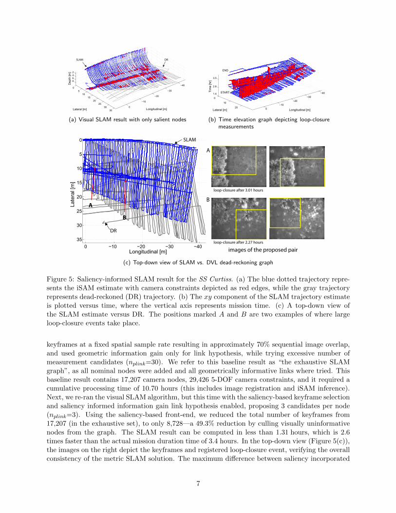
Figure 5: Saliency-informed SLAM result for the SS Curtiss. (a) The blue dotted trajectory repre-sents the iSAM estimate with camera constraints depicted as red edges, while the gray trajectoryrepresents dead-reckoned (DR) trajectory. (b) The xy component of the SLAM trajectory estimateis plotted versus time, where the vertical axis represents mission time. (c) A top-down view ofthe SLAM estimate versus DR. The positions marked A and B are two examples of where largeloop-closure events take place.

keyframes at a fixed spatial sample rate resulting in approximately 70% sequential image overlap,and used geometric information gain only for link hypothesis, while trying excessive number ofmeasurement candidates (nplink=30). We refer to this baseline result as “the exhaustive SLAMgraph”, as all nominal nodes were added and all geometrically informative links where tried. Thisbaseline result contains 17,207 camera nodes, 29,426 5-DOF camera constraints, and it required acumulative processing time of 10.70 hours (this includes image registration and iSAM inference).Next, we re-ran the visual SLAM algorithm, but this time with the saliency-based keyframe selectionand saliency informed information gain link hypothesis enabled, proposing 3 candidates per node(nplink=3). Using the saliency-based front-end, we reduced the total number of keyframes from17,207 (in the exhaustive set), to only 8,728—a 49.3% reduction by culling visually uninformativenodes from the graph. The SLAM result can be computed in less than 1.31 hours, which is 2.6times faster than the actual mission duration time of 3.4 hours. In the top-down view (Figure 5(c)),the images on the right depict the keyframes and registered loop-closure event, verifying the overallconsistency of the metric SLAM solution. The maximum difference between saliency incorporated

7

and exhaustive SLAM is 1.10 meters, whereas the DR trajectory shows significantly larger errordue to the navigation drift.

In terms of saliency’s affect on SLAM performance, we note that even with far fewer nodes inthe graph, we were still able to achieve almost the same total number of camera measurementsin the graph. Using only half (50.7%) of the exhaustive graph nodes and a significantly smallernumber of link proposals (3.4%), we achieved important cross-track camera measurements. Foreasier loop-closure visualization, Figure 5(b) shows a time elevation graph of camera registrationconstraints—here the vertical axis indicates elapsed mission time. While saliency ignored SLAMalso shows reduced error over DR, saliency informed SLAM substantially outperforms it by resultingin more (112.4%) verified links and, thus, less error (15%) relative to the baseline exhaustive SLAMresult, even with a smaller number of link proposals. This is because the saliency-ignored SLAMresult failed to obtain critical, cross-track camera measurements that the saliency-informed SLAMsuccessfully achieved.

4 Perception-driven Navigation

As the final step, we introduce robotic autonomous navigation over an area of interest using thesesaliency metrics. For this type of area coverage mission, a robot needs to explore and map the area,while localizing itself accurately on the map that it builds. This autonomous navigation capabilityinvolves three topics, namely simultaneous localization and mapping (SLAM), path planning, andcontrol. In particular, this thesis considers the task of area coverage (i.e., to cover a certainarea of interest) under the constraint of bounded navigation error. Specifically, our area coverageobjective seeks a balanced control between exploration and revisiting in order to achieve betterSLAM performance. Without loop-closure, SLAM will inevitably accumulate navigation drift overtime; thus, we need to revisit portions of the map to bound error growth. At the same time, weneed to pursue exploration, which is a competing objective that requires mapping the entire areain a reasonable time. Furthermore, and more importantly, SLAM, path planning, and control areinterwoven and, thus, inseparable problems.

4.1 Overview

perception-driven navigation (PDN) consists of three modules: clustering, planning, and rewardevaluation (Figure 6), which will be presented in detail in the following subsections. While the nor-mal SLAM process passively localizes itself and builds a map, PDN (i) clusters salient nodes into aset of candidate revisit waypoints, (ii) plans a point-to-point path for each candidate revisit way-point, and (iii) computes a reward for revisiting each waypoint candidate. The calculated rewardmeasures the utility of revisiting that waypoint (i.e., loop-closure) versus continuing explorationfor area coverage. By comparing the maximum reward for revisiting or exploring, the robot is ableto choose the next best control step.

Given the desired target area coverage (Atarget) and user defined allowable navigation uncer-tainty (Σallow), PDN solves for an intelligent solution to the area coverage planning problem whileconsidering SLAM’s performance. In PDN’s derivation, we address three issues. First, as our ap-proach considers the resulting SLAM performance, the current robot uncertainty should play a rolein the path planning. Thus, the current robot uncertainty is a control parameter that triggers there-planning for better localization and mapping. Second, because the robot should complete thearea coverage mission in a timely manner, the map uncertainty in terms of uncovered area needsto be considered. Finally, PDN needs to be computationally scalable for real-time, real-world per-

8

SLAM- add nodes- add odometry- add camera meas.

PDN- update wps (waypoints)- plan a path to each wp- compute reward (R ) revisit wp = argmax R

Compute saliency

Revisit the k th waypoint

k > 0 ?

yes

nok=0: exploration

cont

inue

on

the

nom

inal

pat

h

kk

k

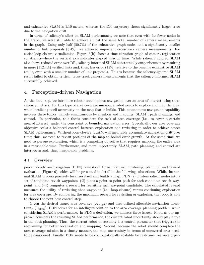
Figure 6: Illustration of PDN’s flow diagram. Provided with a SLAM pose-graph and saliencymap, PDN updates a set of waypoints, plans a path to these waypoints, and computes rewards foreach of the waypoints. The reward Rk is computed for each waypoint k where the reward fromexploration Rexp = R0 corresponds to the 0th waypoint (k = 0). Lastly, either a revisiting orexploration action is executed to yield the maximum reward.

formance. Since the complexity of the algorithm scales linearly with the number of revisit points,maintaining a feasible number of candidate revisit nodes is our focus.Waypoint Generation: Although all nodes in the pose-graph could be considered as waypoints,evaluating the outcome for all possible revisits is impractical. Moreover, due to the uneven spa-tial distribution of feature-rich areas in the environment, not all nodes are visually plausible forloop-closure. Therefore, PDN computes expected rewards for only a subset of candidate nodes se-lected for their visual saliency levels. This waypoint generation consists of two parts: salient nodeclustering and waypoint selection for each cluster. First, we threshold keyframes based upon theirlocal saliency level to generate a set of 3D points with strong local saliency. Then, we cluster lo-cally salient nodes into local neighborhoods, forming clusters, from which we select a representativewaypoint node by considering both its visual uniqueness (i.e., global saliency level) and usefulnessfor loop-closure.Path Generation: For this set of waypoints, the robot computes a shortest path from its currentpose to each waypoint to evaluate the expected reward along that path. We found that, althoughthe surface is curved, applying A* [17] globally on the existing nodes results in a fast and globallyoptimal path on the sample nodes because the nodes are continuously distributed without obstacles.Reward for a Path: Reward for a path is defined in terms of the robot’s navigation uncertaintyand achieved area coverage. We introduce a weighted sum that determines the balance betweenpose uncertainty and area coverage. Although we maximize the reward, the formulation can bemore intuitively understood when we consider each term as a penalty. The navigation uncertaintyterm corresponds to the penalty for SLAM, where the action with minimal uncertainty increase ispreferred. The area coverage metric is the penalty in area coverage when performing an action. Bytaking a weighted sum of these two costs, we can evaluate the total penalty, Ck, for a waypoint k.The reward is the minus of this penalty, and PDN selects an action with the largest reward, or inother words, with the minimal penalty.

Ck = α · Ukrobot + (1− α) · Ak

map (3)

Rk = −Ck (4)

9

r

k WPX

nnΣ

r+1,r+1

exp

k

Σ=Σ

Outbound

InboundRevisit

Exploration

th

: real nodes

: virtual nodes

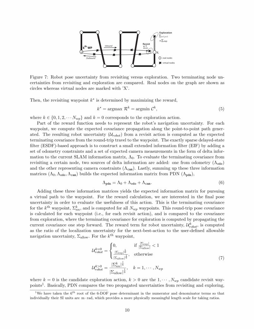
Figure 7: Robot pose uncertainty from revisiting versus exploration. Two terminating node un-certainties from revisiting and exploration are compared. Real nodes on the graph are shown ascircles whereas virtual nodes are marked with ’X’.

Then, the revisiting waypoint k∗ is determined by maximizing the reward,

k∗ = argmax Rk = argmin Ck, (5)

where k ∈ {0, 1, 2, · · ·Nwp} and k = 0 corresponds to the exploration action.Part of the reward function needs to represent the robot’s navigation uncertainty. For each

waypoint, we compute the expected covariance propagation along the point-to-point path gener-ated. The resulting robot uncertainty (Urobot) from a revisit action is computed as the expectedterminating covariance from the round-trip travel to the waypoint. The exactly sparse delayed-statefilter (ESDF)-based approach is to construct a small extended information filter (EIF) by adding aset of odometry constraints and a set of expected camera measurements in the form of delta infor-mation to the current SLAM information matrix, Λ0. To evaluate the terminating covariance fromrevisiting a certain node, two sources of delta information are added: one from odometry (Λodo)and the other representing camera constraints (Λcam). Lastly, summing up these three informationmatrices (Λ0,Λodo,Λcam) builds the expected information matrix from PDN (Λpdn),

Λpdn = Λ0 + Λodo + Λcam. (6)

Adding these three information matrices yields the expected information matrix for pursuinga virtual path to the waypoint. For the reward calculation, we are interested in the final poseuncertainty in order to evaluate the usefulness of this action. This is the terminating covariancefor the kth waypoint, Σk

nn, and is computed for all Nwp waypoints. This round-trip pose covarianceis calculated for each waypoint (i.e., for each revisit action), and is compared to the covariancefrom exploration, where the terminating covariance for exploration is computed by propagating thecurrent covariance one step forward. The reward term for robot uncertainty, Uk

robot, is computedas the ratio of the localization uncertainty for the next-best-action to the user-defined allowablenavigation uncertainty, Σallow. For the kth waypoint,

Uk=0robot =

0, if|Σexp||Σallow| < 1

|Σexp|16

|Σallow|16, otherwise

Uk>0robot =

|Σknn|

16

|Σallow|16

, k = 1, · · · , Nwp

(7)

where k = 0 is the candidate exploration action, k > 0 are the 1, · · · , Nwp candidate revisit way-points1. Basically, PDN compares the two propagated uncertainties from revisiting and exploring,

1We have taken the 6th root of the 6-DOF pose determinant in the numerator and denominator terms so thatindividually their SI units are m · rad, which provides a more physically meaningful length scale for taking ratios.

10

and then chooses the smaller one as in Figure 7. When the expected exploration covariance is belowthe allowable covariance, the cost in the robot pose uncertainty term, U0

robot, is zero, leading therobot to pursue exploration. On the other hand, when the exploration covariance exceeds the allow-able covariance, then the robot pose uncertainty term for exploration, U0

robot, is compared againstall candidate revisit actions, Uk>0

robot, which will be smaller when revisiting is likely to obtain enoughloop-closures to overcome the increased navigation uncertainty from detouring. Unlike previousstudies in active exploration of [18], [19] and [20], where the authors did not consider the actuallikelihood of obtaining perceptual loop-closures, our approach introduces a realistic expectation inthe reward calculation for the likelihood of camera loop-closures based upon visual saliency.

Secondly, we add a bias term for area coverage. The purpose of the mission is to cover atarget area in a timely manner while considering SLAM’s navigation performance. In other words,without an area coverage term, there will be a trivial solution to this problem—to repeatedly revisitto keep the uncertainty very small. To prevent this, the area coverage term for the kth waypointis defined as the ratio of area-to-cover with respect to the target-coverage-area, where the targetarea is provided by the user,

Akmap =

Ato cover

Atarget=Atarget −Acovered +Ak

redundant

Atarget, (8)

Akredundant = redundant coverage by revisiting (9){

= 0, for exploration

= l(Pk) ·D > 0 for revisiting. (10)

Here, l(Pk) is the expected path length added by revisiting the kth waypoint, D is the sensor field ofview width, Atarget is the pre-defined target coverage area as set in the mission planning phase, andAredundant is the expected redundant area coverage produced by a revisiting action. This additionalarea is the result of multiplication of the revisit path with the sensor field of view width and hasnonzero value, Ak

redundant = l(Pk) ·D.

4.2 Implementation and Results

For validation, we present an evaluation of PDN as applied to a hybrid simulation trajectorygenerated from real ship hull inspection data. Since there is no ground-truth available for ourunderwater missions, we use the baseline exhaustive SLAM result from previous chapter to generatea hybrid simulation with preplanned nominal trajectory. In all cases of evaluation, PDN resultsare compared with other traditional preplanned survey schemes, in terms of robot uncertainty (asa measure of SLAM performance) and area coverage rate (as a measure of coverage performance).One pattern is an open-loop control that follows the given nominal trajectory without any revisiting.The other survey pattern is to preplan some deterministic revisit actions during the preplanningphase, which are aimed at achieving any possible loop-closures. This deterministic revisit strategyis typical of underwater vehicle operations, and is passively preplanned or executed by a humanpilot. In this work, we call this preplanned regular revisit “exhaustive revisit”. In the exhaustiverevisit scenario, the vehicle is controlled to come back to a waypoint in every other track-line forpossible loop-closure, regardless of the actual feature distribution in the environment.

4.2.1 PDN with Synthetic Saliency Map

The first set of tests are with a synthetic saliency map imposed over the area with full weight onthe pose uncertainty (α = 1.0). For the exhaustive revisit, the robot is commanded to revisit a

11

Good Saliency Distribution for Exhaustive Revisit

−20−10

010

0 10 20 30 40

02468

Lateral [m]Longitudinal [m]

Dep

th [m

]

(a) Exhaustive

−20−10

010

0 10 20 30 40

02468

Lateral [m]Longitudinal [m]

Dep

th [m

]

(b) PDN

0 200 400 600 800 10000

0.5

1

1.5

2

2.5

3

3.5 x 10−4

386.44m

611.61m

885.96m

Path length [m]

Rob

ot u

ncer

tain

ty

OPLPDNEXH

allowable uncertainty

(c) Pose uncertainty

0 200 400 600 800 10000

0.2

0.4

0.6

0.8

1

Path length [m]

Are

a co

vera

ge

OPLPDNEXH

(d) Area coverage

Poor Saliency Distribution for Exhaustive Revisit

−20−10

010

0 10 20 30 40

02468

Lateral [m]Longitudinal [m]

Dep

th [m

]

(e) Exhaustive

−20−10

010

0 10 20 30 40

02468

Lateral [m]Longitudinal [m]

Dep

th [m

]

(f) PDN

0 200 400 600 800 10000

1

2

3

4

5

6

7

8 x 10−4

386.44m

642.00m

883.62m

Path length [m]

Rob

ot u

ncer

tain

ty

OPLPDNEXH

allowable uncertainty

(g) Pose uncertainty

0 200 400 600 800 10000

0.2

0.4

0.6

0.8

1

Path length [m]

Are

a co

vera

ge

OPLPDNEXH

(h) Area coverage

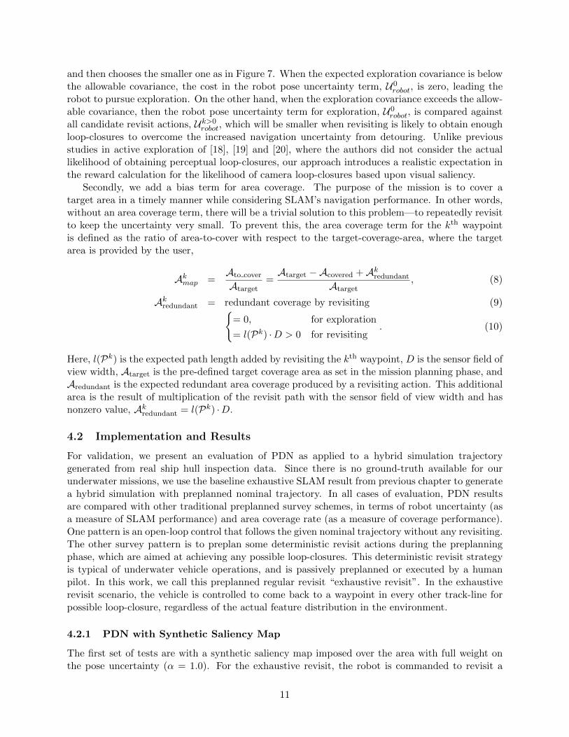
Figure 8: PDN results for biased saliency maps. Similar to the case of uniform distribution, poseuncertainty and area coverage graph are compared for two biased saliency regions among open-loop(green), exhaustive revisit (blue) and PDN (red), where the black dots indicate points when revisitoccurred. Open-loop and PDN perform the same as in the evenly distributed salient region case.However, exhaustive revisit strongly depends on the spatial distribution of feature-rich areas.

point on the first track-line in every other track-line it travels. In this test, the exhaustive revisithappens on a line on the bottom of the hull. Because this repeated visit is preplanned withoutknowing the actual visual feature distribution in the environment, we assign the same exhaustiverevisit control for all cases.

In this test, we show cases where the feature-rich distribution is biased to show how the pre-planned exhaustive revisit succeeds and fails depending on the saliency distribution. When all ofthe exhaustive revisit paths land on the salient region (Figure 8(a)), the likelihood of obtainingloop-closure during the revisit is higher, and the exhaustive revisit achieves tightly bounded uncer-tainty for the robot pose (Figure 8(c)). On the other hand, when none of the revisit paths are onsalient regions, as in the case of Figure 8(e), the algorithm basically performs worse than open-loop.Without meaningful loop-closures on the revisit, the control just increases the overall path lengthand slows coverage rate, as can be seen in Figure 8(g) and Figure 8(h). Unfortunately, the salientregion distribution cannot be known a priori when the preplanning takes place. Note that for bothcases, the total path length and the area coverage rate stays the same for the exhaustive revisitsince it is preplanned. On the other hand, from PDN’s point of view, there is no difference betweenall three cases, resulting in a consistent performance on uncertainty bounding and area coverage.

4.2.2 PDN with Real Image Data

We now evaluate PDN for saliency-informed SLAM using real underwater images for a cameramission profile. The saliency map is generated and updated online from the real underwater imagesthat are available from the baseline result. Using the pair of real-world images, the saliency scoreand camera registration engine are applied as in the normal saliency-informed SLAM process. Aweight factor of α = 0.75 is selected in PDN to impose a biased weight on the pose-uncertaintyrather than area coverage. Similar to the synthetic saliency case, the uncertainty and area coveragegraph for PDN is compared with open-loop (OPL) and exhaustive (EXH) revisit. Based upon the

12

0 500 1000 1500 2000 25000

1

2

3

4

5

6x 10−4

1244.02m

1556.75m

2476.31m

Path length [m]

Rob

ot u

ncer

tain

ty

OPLPDNEXH

1 2 3 4 5 6 7 98 allowable uncertainty

(a) Pose uncertainty

−20

−10

0

0 10 20 30

02468

Lateral [m]Longitudinal [m]

Dep

th [m

]

(b) Trajectory (EXH)

−20

−10

0

0 10 20 30

02468

Lateral [m]Longitudinal [m]

Dep

th [m

]

(c) Trajectory (PDN)

0 500 1000 1500 2000 25000

0.1

0.2

0.3

0.4

0.5

0.6

0.7

0.8

0.9

1

Path length [m]

Are

a co

vera

ge

OPLPDNEXH

(d) Area coverage

−20−10

0

5 10 15 20 25

Longitudinal [m]Lateral [m]

Tim

e

(e) Time elevation (EXH)

−20−10

0

5 10 15 20 25

Longitudinal [m]Lateral [m]

Tim

e

(f) Time elevation (PDN)

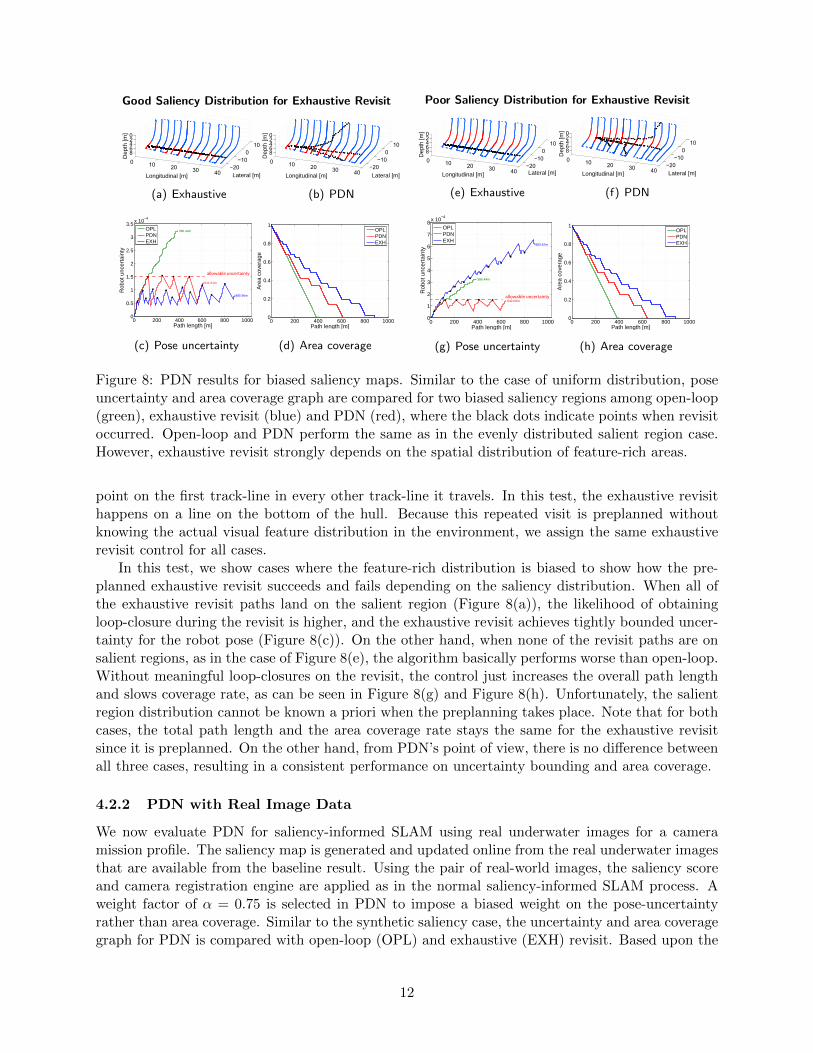
Figure 9: PDN for saliency-informed SLAM on a camera mission. Similar to the synthetic saliencycase, (a) and (d) show the pose uncertainty and area coverage with respect to the path length. Intrajectories (b) and (c), nodes are color-coded by their saliency level from the real images. Theexhaustive revisit was preplanned over the salient band, however, PDN is able to find this sameoptimal path to follow as in (c). In the time elevation graphs ((e) and (f)), PDN shows a comparablenumber of successful loop-closures to the exhaustive revisit.

knowledge of the saliency distribution in the baseline result, we preplanned the exhaustive revisitpath to be laid over the salient band to provide the best possible case to be compared with PDN.Because the exhaustive revisit is intentionally planned over the salient region, the resulting graphof exhaustive revisit shows the maximum SLAM performance—maintaining low uncertainty, butproducing an exceeding number of revisits and longer path length.

Uncertainty change and the area coverage rate are presented in Figure 9(a) and (d) for bothtypes of missions. As shown in Figure 9(c), PDN followed trajectories to obtain expected vi-sual loop-closures to reduce the uncertainty whenever it exceeded the allowable covariance bound.Specifically, exhaustive revisits in the camera mission result in 47 revisit actions with twice thetotal path length of the nominal trajectory. Assuming a constant speed for the vehicle, this ex-haustive revisit strategy would double the overall mission time. In this camera mission, note thatthe number of revisits by PDN (9) is substantially smaller than the exhaustive revisit case. PDNpresents a result with less number of revisits while maintaining full control on the uncertainty level,and still achieving the important loop-closures. The loop-closing camera measurements are clearlyillustrated in the time elevation graph of Figure 9(e) and (f). The red lines in the graph depictthe camera measurements made by the loop-closures. As can be seen in the time elevation graphs,PDN obtained a similar number of loop-closures as compared to the exhaustive revisit case.

13

5 Conclusion

This thesis proposed an integrated approach toward robotic navigation and exploration for au-tonomous robot missions. SLAM and path planning have traditionally been considered as twoseparate problems, each assuming some prior information from the other. This thesis started fromthe viewpoint of SLAM and presented a metric for visual saliency that could be used with geo-metric information to improve loop-closure performance. This saliency-informed SLAM result wasthen combined with planning to lead the robot autonomously along trajectories that yielded bet-ter SLAM results and survey area coverage. Experiments using real underwater mission data andsimulations were provided from several different vessels to evaluate the reported algorithms.

Contributions of this thesis includes (i) Real-time visual SLAM is developed and successfullyapplied to a real-world AUV ship hull inspection application. Specifically, a monocular cameraimage registration engine is developed and integrated into a real-time SLAM implementation. (ii)Developed two novel measures of visual saliency that improve underwater visual SLAM. Localsaliency measures texture richness of a scene and aids keyframe selection. Global saliency detectsrarity of a scene. (iii) A novel solution for concurrent SLAM and planning for the robotic areacoverage problem, called PDN is developed. PDN is an integrated navigation algorithm that au-tomatically achieves efficient target area coverage while maintaining good visual SLAM navigationperformance. PDN provides an intelligent and fully autonomous online control scheme for efficientbounded-error area coverage that strikes a balance between revisit and exploration actions in adecision theoretic way.

References

[1] R. Sim and N. Roy, “Global a-optimal robot exploration in SLAM,” in Proc. of the IEEE Intl.Conf. on Robotics and Automation, Barcelona, Spain, 2005, pp. 661–666.

[2] R. M. Eustice, H. Singh, J. J. Leonard, and M. R. Walter, “Visually mapping the RMSTitanic: Conservative covariance estimates for SLAM information filters,” Intl. Journal ofRobotics Research, vol. 25, no. 12, pp. 1223–1242, 2006.

[3] J. Vaganay, M. Elkins, D. Esposito, W. O’Halloran, F. Hover, and M. Kokko, “Ship hullinspection with the HAUV: U.S. Navy and NATO demonstrations results,” in Proc. of theIEEE/MTS OCEANS Conf. and Exhibition, Boston, MA, 2006, pp. 1–6.

[4] K. Zuiderveld, “Contrast limited adaptive histogram equalization,” in Graphics Gems IV,P. Heckbert, Ed. Boston: Academic Press, 1994, vol. IV, pp. 474–485.

[5] D. Lowe, “Distinctive image features from scale-invariant keypoints,” Intl. Journal of Comp.Vision, vol. 60, no. 2, pp. 91–110, 2004.

[6] H. Bay, A. Ess, T. Tuytelaars, and L. Van Gool, “Speeded-up robust features (SURF),” Comp.Vision and Image Understanding, vol. 110, no. 3, pp. 346–359, 2008.

[7] R. M. Eustice, O. Pizarro, and H. Singh, “Visually augmented navigation for autonomousunderwater vehicles,” IEEE Journal of Oceanic Engineering, vol. 33, no. 2, pp. 103–122, Apr.2008.

[8] N. Carlevaris-Bianco and R. M. Eustice, “Multi-view registration for feature-poor underwaterimagery,” in Proc. of the IEEE Intl. Conf. on Robotics and Automation, Shanghai, China,May. 2011, pp. 423–430.

14

[9] A. Kim and R. M. Eustice, “Pose-graph visual SLAM with geometric model selection forautonomous underwater ship hull inspection,” in Proc. of the IEEE/RSJ Intl. Conf. on Intell.Robots and Syst., St. Louis, MO, Oct. 2009, pp. 1559–1565.

[10] P. Torr, “Model selection for two view geometry: A review,” in Shape, Contour and Groupingin Comp. Vision. Springer, 1999, pp. 277–301.

[11] B. Horn, “Relative orientation revisited,” Journal of the Optical Society of America A, vol. 8,no. 10, pp. 1630–1638, Oct 1991.

[12] R. Haralick, “Propagating covariance in computer vision,” in Proc. of the Intl. Conf. PatternRecognition, vol. 1, Jerusalem, Israel, Oct. 1994, pp. 493–498.

[13] K. S. Jones, “A statistical interpretation of term specificity and its application in retrieval,”Journal of Documentation, vol. 28, pp. 11–21, 1972.

[14] G. Salton and C. S. Yang, “On the specification of term values in automatic indexing,” Journalof Documentation, vol. 29, pp. 351–372, 1973.

[15] S. Robertson, “Understanding inverse document frequency: On theoretical arguments for idf,”Journal of Documentation, vol. 60, pp. 503–520, 2004.

[16] V. Ila, J. Porta, and J. Andrade-Cetto, “Information-based compact pose SLAM,” IEEETransaction on Robotics, vol. 26, no. 1, pp. 78–93, Feb. 2010.

[17] S. J. Russell and P. Norvig, Artificial Intelligence: A Modern Approach. Pearson Education,2003.

[18] F. Bourgault, A. A. Makarenko, S. B. Williams, B. Grocholsky, and H. F. Durrant-Whyte,“Information based adaptive robotic exploration,” in Proc. of the IEEE/RSJ Intl. Conf. onIntell. Robots and Syst., 2002, pp. 540–545.

[19] A. A. Makarenko, S. B. Williams, F. Bourgault, and H. F. Durrant-Whyte, “An experimentin integrated exploration,” in Proc. of the IEEE/RSJ Intl. Conf. on Intell. Robots and Syst.,2002, pp. 534–539.

[20] C. Stachniss, G. Grisetti, and W. Burgard, “Information gain-based exploration using rao-blackwellized particle filters,” in Proc. of the Robotics: Science & Syst. Conf., Cambridge,MA, USA, 2005.

15