Active Versus Passive: Receiver Model Transformsfor Diffusive Molecular Communication

Adam Noel∗†, Yansha Deng‡, Dimitrios Makrakis†, and Abdelhakim Hafid∗∗Department of Computer Science and Operations Research, University of Montreal†School of Electrical Engineering and Computer Science, University of Ottawa

‡Department of Informatics, King’s College London

Abstract—This paper presents an analytical comparison ofactive and passive receiver models in diffusive molecular com-munication. In the active model, molecules are absorbed whenthey collide with the receiver surface. In the passive model, thereceiver is a virtual boundary that does not affect moleculebehavior. Two approaches are presented to derive transformsbetween the receiver signals. As an example, two models foran unbounded diffusion-only molecular communication systemwith a spherical receiver are unified. As time increases in thethree-dimensional system, the transform functions have constantscaling factors, such that the receiver models are effectivelyequivalent. Methods are presented to enable the transformationof stochastic simulations, which are used to verify the transformsand demonstrate that transforming the simulation of a passivereceiver can be more efficient and more accurate than the directsimulation of an absorbing receiver.

I. INTRODUCTION

Molecular communication has been receiving increasingattention as a strategy for the design of novel communicationsystems in fluid environments; see [1]. Much of this attentionhas been focused on molecular communication via diffusion,whose attractive properties include no required external energyor infrastructure for the molecules to propagate from a trans-mitter. Once molecules are released by the transmitter, theymove in the fluid via a process that is effectively random.

Arguably one of the biggest schisms in the analysis ofcommunication via diffusion is in the modeling of the receiver.Receiver models are generally classified as either passiveor active. A passive receiver can observe but has no effecton molecule behavior. An active receiver is typically a sitefor chemical reactions, either inside or on its surface, andmolecules can be identified when a reaction takes place. Pas-sive receiver models are commonly favored for their simplicityin analysis and simulation, whereas active models are morerealistic in representing the chemical detection of molecules.

The vast majority of studies of single communication linksassumes a receiver model and then proceeds without assessingthe choice. For example, active receivers have been consideredin [2], [3], and passive receivers have been considered in [4]and the first author’s work in [5]. Explicit comparisons be-tween receiver models are very uncommon; one example is [6],where the one-dimensional passive and absorbing models wereboth fitted to experimental data obtained from the tabletoptestbed in [7]. The authors observed similarities between thetwo models and attributed them to the dominance of airflow.

Other authors, such as in [8], [9], derived results that werevalid for any model but did not compare models directly.

In this work, we compare active and passive receiver mod-els. Our goal is to unify the models so that we can transformsignals from one model to the other. As an example, weunify the channel impulse responses (CIRs) for a sphericalreceiver in an unbounded diffusion-only environment. Otherrealistic phenomena, such as fluid flow or the potential forother chemical reactions, may be considered in future work.We consider both a perfectly-absorbing receiver and a passivereceiver in three dimensions (3D) and in one dimension (1D,i.e., the receiver is treated as a line segment). All of thesesystems have been studied extensively, and we omit the two-dimensional environment because the CIR of the absorbingcircle has not been described in closed form; see [1]. Bycarefully choosing how to represent the CIRs, we derivefunctions that transform a signal at a passive receiver intoa signal at the corresponding absorbing receiver. In particular,we make the following contributions:

1) We take the integral of the passive CIR so that it includesprior signal information and is then comparable to theactive CIR. In practice, this can be measured usingthe weighted sum detector that we introduced in [5].Alternatively, we take the derivative of the active CIR sothat it is an instantaneous measurement to compare withthe passive CIR. The derivative can be obtained fromthe hitting rate detector proposed in [10]. These twoapproaches, which lead us to derive transform functionsfor the 1D and 3D environments, apply to absorbing andpassive receivers in any environment.

2) We describe the proper implementation of the energydetector at a passive receiver and the hitting rate detectorat an absorbing receiver to perform the integral andderivative operations, respectively. These detector mod-ifications are needed to accurately apply the transformsbetween active and passive signals in simulations.

3) We demonstrate the accuracy of the transforms andtheir inverses, both analytically and via simulation. As aresult, we can work with whichever model is currentlymost appropriate and then accurately transform the sig-nal to the other model.

By deriving transforms between the passive and theperfectly-absorbing receiver models for the sphere in a

arX

iv:1

604.

0459

5v2

[cs

.ET

] 1

0 Se

p 20

16

diffusion-only system, we effectively unify all existing liter-ature that has selected one of these models. This unificationmakes the initial selection of a receiver model less critical. Wecan analyze one model and then simulate the other model, ordivide the analysis between the two models, as desired, whichgives us greater flexibility when deciding which model to use.As an example, we show that it can be both more accurateand more efficient to simulate an absorbing receiver signal bytransforming a passive receiver simulation instead of directlysimulating the absorbing receiver. This is due to the latter’srequirement of a very small simulation time step for accuracy.

We also note that our analysis focuses on expected CIRs.The impact of the transform functions on the channel statisticswill be considered in future work. However, we verify thetransforms numerically and also using average results ob-tained from our particle-based stochastic molecular communi-cations simulator AcCoRD (Actor-based Communication viaReaction-Diffusion), which is available as a public beta [11].

The rest of this paper is organized as follows. Section IIdescribes the system models and presents the correspondingCIRs. In Section III, we derive the transform functions. InSection IV, we discuss the implementation of the integral andderivative operations. We verify our analytical results withsimulations in Section V, and conclude in Section VI.

II. SYSTEM MODEL AND CHANNEL IMPULSE RESPONSES

We consider a point transmitter (TX) releasing N moleculesinto an unbounded 1D or 3D environment. We assume uni-form temperature and viscosity, and that the local moleculeconcentration is sufficiently low, so that molecules diffuse withconstant diffusion coefficient D. These molecules are observedby a receiver (RX) that is centered at a distance d from theTX and has radius rRX, i.e., a segment of length 2rRX in 1Dand a sphere in 3D. If the RX is active, then we consider aperfectly-absorbing surface that removes and counts moleculesas they arrive, i.e., the absorption rate is k →∞. If the RX ispassive, then it has no impact on molecule behavior but is ableto count the number of molecules within its virtual boundaryat any instant. Finally, we assume that diffusion is the onlyphenomenon affecting molecule behavior in the propagationenvironment (except for absorption at the active RX’s surface).

We define the channel impulse response (CIR) NRX (t) asthe number of molecules expected at the RX at time t, giventhat N molecules are instantaneously released by the TX attime t = 0. In the remainder of this section, we present theCIRs that are used throughout the remainder of this paper.

A. 3D Channel Impulse Responses

If the environment is 3D, then the CIR of the absorbing RXis given by [12, Eq. (23)]

NRX (t) |AB3D =

NrRX

derfc

(d− rRX√

4Dt

), (1)

where erfc (x) = 1 − erf (x) is the complementary errorfunction (from [13, Eq. (8.250.4)]), and the “AB” superscriptmeans “absorbing”. Eq. (1) describes the total number of

molecules absorbed by time t. For the passive RX, theexpected point concentration Cpoint (t) is [14, Eq. (4.28)]

Cpoint (t) |PA3D =

N

(4πDt)3/2exp

(− d2

4Dt

), (2)

where we use the “PA” superscript to denote “passive”.It is common to assume that the molecule concentration

is uniform inside a passive RX, which is justified if the RXis sufficiently far from the TX, i.e., if d � rRX (as wedemonstrated in [15]). Here, we make this assumption for easeof analysis. Thus, we multiply (2) by the RX volume VRX towrite the number of molecules expected inside the RX as

NRX (t) |PA3D =

NVRX

(4πDt)3/2exp

(− d2

4Dt

). (3)

B. 1D Channel Impulse Responses

If the environment is 1D, then the CIR of the absorbing RXis given by [1, Eq. (7)]

NRX (t) |AB1D = Nerfc

(d− rRX√

4Dt

). (4)

The expected point concentration for the 1D passive RX is[14, Eq. (3.6)]

Cpoint (t) |PA1D =

N√4πDt

exp

(− d2

4Dt

). (5)

If we assume that the passive RX is sufficiently far fromthe TX, then the simplified 1D CIR is directly from (5) as

NRX (t) |PA1D =

rRXN√πDt

exp

(− d2

4Dt

). (6)

III. UNIFYING RECEIVER MODELS

In this section, we seek the existence of transform functionsthat have the form

Absorbing Signal ?= S(Passive Signal), (7)

where we emphasize that we are most interested in obtainingan active RX signal from a passive RX, since a passive RX isgenerally faster to simulate (though simulating absorption canbe faster if most molecules get absorbed). We do not constrainthe “signals” in (7) to be CIRs; rather, we seek to manipulateeither the absorbing or the passive CIR so that it is comparableto the other.

We claim that the CIRs of the two receiver models canbe perceived as similar measurements but they provide funda-mentally different information about what has happened at theRX. A sample of the absorbing RX’s CIR is the total numberof molecules that have arrived at that RX since they werereleased by the TX, i.e., a sample includes history information.However, a sample of the passive RX’s CIR is only the currentnumber of molecules that are inside the RX at the instant whenthe sample is taken; the history of the molecules that haveentered and left the passive RX is ignored. So, to derive atransform, we propose using either a passive receiver modelthat accounts for signal “history”, or an active receiver modelthat describes the instantaneous behavior.

We first consider the 3D environment, where we derivethe transform function that applies to the passive signal withhistory information, S ′3D, and that which applies to the instan-taneous passive signal, S ′′3D. These transforms will simplifyto constant scaling factors in the asymptotic case, i.e., ast → ∞, which may be useful for modeling intersymbolinterference (ISI). Then, we consider the 1D environment,where the corresponding transform functions are S ′1D and S ′′1D.

A. 3D Analysis

We begin our 3D analysis with the more intuitive signalmanipulation, which is to model the receiver as an energydetector. The CIR of the absorbing RX is intuitively a measureof the received energy over time, since the signal accounts forevery molecule arrival. Analytically, an energy detector forthe passive RX is defined by integrating the CIR over time,and we will show in Section IV that this can be implementedwith a weighted sum detector. Analogously to [14, Eq. (3.5b)],which derives the instantaneous signal due to a point sourcethat is continuously releasing molecules, we can integrate (3)over t to write the energy detector signal ED (t) as

ED (t) |PA3D =

NVRX

4πDderfc

(d√4Dt

). (8)

We can immediately compare (8) with the absorbing CIRin (1), even though there is an abuse of notation since (1) hasunit [mol] (i.e., molecule) whereas (8) has units [mol · s]. Thisdifference is a side effect of having physically different RXs.To write (8) as a function of (1), we need a way to separatethe terms inside the complementary error function in (1). Todo this, we will use the elementary approximation of erf (x)in [16, Eq. (4a)], which we have observed to have a relativeerror of less than 1% for 0 ≤ x ≤ 2.5, to re-write erfc (x) as

erfc (x) ≈ exp

(−16

23x2 − 2√

πx

), (9)

and therefore write erfc (·) in (1) as

erfc

(d− rRX√

4Dt

)≈ erfc

(d√4Dt

)A(t), (10)

where we define the function A(t) as

A(t) = exp

(rRX√Dt

(4(2d− rRX)

23√Dt

+1√π

)), (11)

and in practice (10) is very accurate unless t is very small.Using (10) and the equation for the volume of a sphere, wewrite the transform function S ′3D as

NRX (t) |AB3D = S ′3D(ED (t) |PA

3D) ≈ 3DA(t)

r2RX

ED (t) |PA3D, (12)

and we can re-arrange (12) to find the inverse transform S ′−13D .

In the asymptotic case, i.e., as t →∞, the complementaryerror function goes to 1 and thus the transform function S ′∞3Dhas a constant scaling factor

NRX (t) |AB3D = S ′∞3D (ED (t) |PA

3D) ≈ 3D

r2RX

ED (t) |PA3D. (13)

From (13), we see that these two fundamentally differentreceiver models are effectively equivalent (asymptotically).

Next, we perform the complementary signal manipulation,i.e., we seek a measure of the instantaneous behavior of theabsorbing receiver model to compare with the passive RX CIR.Thus, we take the derivative of the active RX’s CIR. This isthe rate of molecule absorption at the RX, ∆NRX (t), and hasbeen previously presented as [12, Eq. (22)]

∆NRX (t) |AB3D =

NrRX(d− rRX)

d√

4πDt3exp

(− (d− rRX)2

4Dt

).

(14)The implementation of (14) in simulations will be discussed

in Section IV. Here, we can compare (14) with (3) (once againwith a slight abuse of notation since (14) is in [mol · s−1] and(3) is in [mol]). From the properties of exponential functions,it can be shown that the transform function S ′′3D is

∆NRX (t) |AB3D =S ′′3D(NRX (t) |PA

3D)

=3D(d− rRX)

r2RXd

NRX (t) |PA3D

× exp

(rRX(2d− rRX)

4Dt

), (15)

Asymptotically, the transform function S ′′∞3D has a constantscaling factor, i.e.,

∆NRX (t) |AB3D =S ′′∞3D (NRX (t) |PA

3D)

≈ 3D(d− rRX)

r2RXd

NRX (t) |PA3D, (16)

and if we again assume that the TX is sufficiently far fromthe RX (i.e., d � rRX), then the two asymptotic transformfunctions S ′∞3D and S ′′∞3D are analogous for the 3D receivermodels with the same scaling factor, i.e., 3D/r2

RX.

B. 1D Analysis

Our strategy to transform between the active and passivereceiver models in the 1D system is the same as that appliedfor the 3D system. The energy detector signal for the 1Dsystem can be obtained by integrating the passive CIR in (6)over time. If we use τ as the dummy variable of integrationover time, then we can integrate (6) via the substitutionx = τ−

12 , the integral [13, Eq. (2.325.12)]∫

1

x2exp

(−ax2

)dx = −

exp(−ax2

)x

+√aπ erf

(−√ax),

(17)

and the definition of erfc (x). By performing these steps, wederive the expected energy detector signal at the 1D passiveRX as

ED (t) |PA1D = 2rRXN

[√t

πDexp

(− d2

4Dt

)− d

2Derfc

(d√4Dt

)]. (18)

We compare (18) with the 1D absorbing CIR in (4). We doso to obtain the transform function S ′1D as

NRX (t) |AB1D =S ′1D(ED (t) |PA

1D)

=2DA(t)

d

[N

√t

πDexp

(− d2

4Dt

)− ED (t) |PA

1D

2rRX

], (19)

where A(t) is in (11). As t →∞, the transform becomes

NRX (t) |AB1D =S ′∞1D (ED (t) |PA

1D)

≈ 2D

d

[N

√t

πD− ED (t) |PA

1D

2rRX

], (20)

which does not have a constant scaling factor.Finally, we determine the transform function S ′′1D. The

derivative of the CIR at the 1D absorbing RX in (4) is therate of molecule absorption at, and from [1, Eq. (6)] is

∆NRX (t) |AB1D =

N(d− rRX)√4πDt3

exp

(− (d− rRX)2

4Dt

). (21)

We can compare (21) with (6) to derive the transformfunction S ′′1D as

∆NRX (t) |AB1D =S ′′1D(NRX (t) |PA

1D)

=d− rRX

2rRXtNRX (t) |PA

1D exp

(rRX(2d− rRX)

4Dt

),

(22)

which closely resembles its 3D variant S ′′3D in (15). However,one key difference is that it does not have a constant scalingfactor in the asymptotic case, i.e.,

∆NRX (t) |AB1D = S ′′∞1D (NRX (t) |PA

1D) ≈ d− rRX

2rRXtNRX (t) |PA

1D.

(23)The 1D and 3D environments that we considered have

very similar configurations but resulted in different transformfunctions to convert between the active and passive receivermodels. For reference, we have summarized the equations forthe signals and their transforms in Table I. We note that theeffective equivalence (via the constant scaling factor 3D/r2

RX)that we observed for the 3D model in the asymptotic case wasnot observed for the 1D model. Even though each transformfunction only applies to its corresponding system model, ourapproach to derive the transform functions could be appliedto any system model where comparable CIRs can be found.

IV. IMPLEMENTATION DETAILS

In this section, we briefly describe how to measure theenergy and absorption rate detector signals so that we canverify the transforms for active and passive receivers viasimulations. To do so, we need to accommodate discrete (andnoisy) observations of the CIRs and not just the analyticalexpressions in Section II. We assume that, for either receivermodel, the RX takes M samples between time t = 0 andtime t = T . The samples are equally spaced in time by

TABLE ISUMMARY OF ANALYTICAL EXPRESSIONS, WHICH ARE SORTED

ACCORDING TO THE LABELED CURVES IN THE FIGURES IN SECTION V.EQUATIONS DENOTED WITH “∗” ARE NOT SHOWN IN ANY FIGURE.

Curve Signal System 1 System 2

Analytical

Passive CIR (3) (6)Passive ED (8) (18)∗

Absorbing CIR (1) (4)∗

Absorption Rate (14) (21)

Analyticalvia Transform

Passive CIR (15)−1 (22)−1

Passive ED (12)−1 (19)−1∗

Absorbing CIR (12) (19)∗

Absorption Rate (15) (22)

AsymptoticTransform Analytical

Passive CIR (16)−1 (23)−1

Passive ED (13)−1 (20)−1∗

Absorbing CIR (13) (20)∗

Absorption Rate (16) (23)

sampling interval ∆tM = T/M . The individual sample takenat time tm is labeled as NRX (tm), where tm = m∆tM ,m ∈ {1, 2, . . . ,M}.

First, we consider the energy detector. Energy detection bya passive RX has been analyzed in [4], [17] by integratingthe continuous CIR (e.g., (8)). To accommodate discreteobservations, we consider the weighted sum detector that weintroduced in [5, Eq. (37)], where the weighted sum is

M∑m=1

wmNRX (tm) , (24)

and wm is the mth weight. In [5], we described the equalweight detector, where wm = 1∀m, as analogous to an energydetector. However, the corresponding sum is not precisely anenergy detector. To be an energy detector, each sample mustalso be scaled by the sampling interval ∆tM (as done in [18]).If not, then we can artificially detect more energy if we takemore samples over the same sampling interval. By includingthe sampling interval, we design the discrete energy detectorfor the passive RX ED (·) |PA as

ED(tm +

∆tM2

) ∣∣∣PA= ∆tM

m∑l=1

NRX (tl) , (25)

which applies to any environment, and we add the shift∆tM

2 to the energy detector observation time because the lthsample accounts for the energy in the continuous interval[tl − ∆tM

2 , tl + ∆tM2 ].

The net number of absorbed molecules is used in [10] as anabsorption rate detector, but the number of molecules arrivingover the interval [tm, tm+1], i.e.,

NRX (tm+1)−NRX (tm) , (26)

is only a legitimate rate if we divide the difference by the sam-pling interval. Therefore, to be consistent with the absorptionrate, we design the absorption rate detector ∆NRX (·) |AB as

∆NRX

(tm +

∆tM2

) ∣∣∣AB=NRX (tm+1)−NRX (tm)

∆tM, (27)

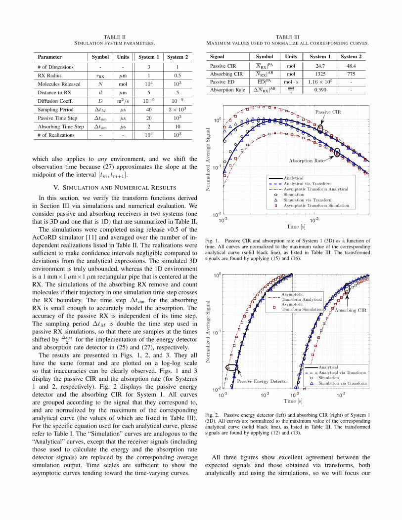
TABLE IISIMULATION SYSTEM PARAMETERS.

Parameter Symbol Units System 1 System 2

# of Dimensions - - 3 1

RX Radius rRX µm 1 0.5

Molecules Released N mol 104 103

Distance to RX d µm 5 5

Diffusion Coeff. D m2/s 10−9 10−9

Sampling Period ∆tM µs 40 2× 103

Passive Time Step ∆tsim µs 20 103

Absorbing Time Step ∆tsim µs 2 10

# of Realizations - - 104 103

which also applies to any environment, and we shift theobservation time because (27) approximates the slope at themidpoint of the interval [tm, tm+1].

V. SIMULATION AND NUMERICAL RESULTS

In this section, we verify the transform functions derivedin Section III via simulations and numerical evaluation. Weconsider passive and absorbing receivers in two systems (onethat is 3D and one that is 1D) that are summarized in Table II.

The simulations were completed using release v0.5 of theAcCoRD simulator [11] and averaged over the number of in-dependent realizations listed in Table II. The realizations weresufficient to make confidence intervals negligible compared todeviations from the analytical expressions. The simulated 3Denvironment is truly unbounded, whereas the 1D environmentis a 1 mm×1µm×1µm rectangular pipe that is centered at theRX. The simulations of the absorbing RX remove and countmolecules if their trajectory in one simulation time step crossesthe RX boundary. The time step ∆tsim for the absorbingRX is small enough to accurately model the absorption. Theaccuracy of the passive RX is independent of its time step.The sampling period ∆tM is double the time step used inpassive RX simulations, so that there are samples at the timesshifted by ∆tM

2 for the implementation of the energy detectorand absorption rate detector in (25) and (27), respectively.

The results are presented in Figs. 1, 2, and 3. They allhave the same format and are plotted on a log-log scaleso that inaccuracies can be clearly observed. Figs. 1 and 3display the passive CIR and the absorption rate (for Systems1 and 2, respectively). Fig. 2 displays the passive energydetector and the absorbing CIR for System 1. All curvesare grouped according to the signal that they correspond to,and are normalized by the maximum of the correspondinganalytical curve (the values of which are listed in Table III).For the specific equation used for each analytical curve, pleaserefer to Table I. The “Simulation” curves are analogous to the“Analytical” curves, except that the receiver signals (includingthose used to calculate the energy and the absorption ratedetector signals) are replaced by the corresponding averagesimulation output. Time scales are sufficient to show theasymptotic curves tending toward the time-varying curves.

TABLE IIIMAXIMUM VALUES USED TO NORMALIZE ALL CORRESPONDING CURVES.

Signal Symbol Units System 1 System 2

Passive CIR NRX|PA mol 24.7 48.4

Absorbing CIR NRX|AB mol 1325 775

Passive ED ED|PA mol · s 1.16× 105 -

Absorption Rate ∆NRX|AB mols 0.390 -

Time [s]10

-310

-2

Normalized

Average

Signal

10-2

10-1

100

Analytical

Analytical via Transform

Asymptotic Transform Analytical

Simulation

Simulation via Transform

Asymptotic Transform Simulation

Absorption Rate

Passive CIR

Fig. 1. Passive CIR and absorption rate of System 1 (3D) as a function oftime. All curves are normalized to the maximum value of the correspondinganalytical curve (solid black line), as listed in Table III. The transformedsignals are found by applying (15) and (16).

Time [s]10

-310

-2

Normalized

Average

Signal

10-2

10-1

100

10-3

10-2

AsymptoticTransform AnalyticalAsymptoticTransform Simulation

Analytical

Analytical via Transform

Simulation

Simulation via TransformPassive Energy Detector

Absorbing CIR

Fig. 2. Passive energy detector (left) and absorbing CIR (right) of System 1(3D). All curves are normalized to the maximum value of the correspondinganalytical curve (solid black line), as listed in Table III. The transformedsignals are found by applying (12) and (13).

All three figures show excellent agreement between theexpected signals and those obtained via transforms, bothanalytically and using the simulations, so we will focus our

Time [s]10

-210

-1

Normalized

Average

Signal

10-1

100

Analytical

Analytical via Transform

Asymptotic Transform Analytical

Simulation

Simulation via Transform

Asymptotic Transform Simulation

Absorption Rate

Passive CIR

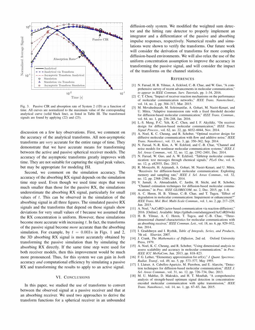
Fig. 3. Passive CIR and absorption rate of System 2 (1D) as a function oftime. All curves are normalized to the maximum value of the correspondinganalytical curve (solid black line), as listed in Table III. The transformedsignals are found by applying (22) and (23).

discussion on a few key observations. First, we comment onthe accuracy of the analytical transforms. All non-asymptotictransforms are very accurate for the entire range of time. Theydemonstrate that we have accurate means for transformingbetween the active and passive spherical receiver models. Theaccuracy of the asymptotic transforms greatly improves withtime. They are not suitable for capturing the signal peak values,but may be appropriate for modeling ISI.

Second, we comment on the simulation accuracy. Theaccuracy of the absorbing RX signal depends on the simulationtime step used. Even though we used time steps that weremuch smaller than those for the passive RX, the simulationsunderestimate the absorbing RX signal, particularly for smallvalues of t. This can be observed in the simulation of theabsorbing signal in all three figures. The simulated passive RXsignals and the transforms that depend on those signals showdeviations for very small values of t because we assumed thatthe RX concentration is uniform. However, these simulationsbecome more accurate with increasing t. In fact, the transformsof the passive signal become more accurate than the absorbingsimulation. For example, by t = 0.003 s in Figs. 1 and 2,the 3D absorbing RX signal is more accurately obtained bytransforming the passive simulation than by simulating theabsorbing RX directly. If the same time step were used forboth receiver models, then this improvement would be muchmore pronounced. Thus, for this system we can gain in bothaccuracy and computational efficiency by simulating a passiveRX and transforming the results to apply to an active signal.

VI. CONCLUSIONS

In this paper, we studied the use of transforms to convertbetween the observed signal at a passive receiver and that atan absorbing receiver. We used two approaches to derive thetransform functions for a spherical receiver in an unbounded

diffusion-only system. We modified the weighted sum detec-tor and the hitting rate detector to properly implement anintegrator and a differentiator of the passive and absorbingimpulse responses, respectively. Numerical results and simu-lations were shown to verify the transforms. Our future workwill consider the derivation of transforms for more complexdiffusion-based environments. We will also relax the use of theuniform concentration assumption to improve the accuracy intransforming the passive signal, and will consider the impactof the transforms on the channel statistics.

REFERENCES

[1] N. Farsad, H. B. Yilmaz, A. Eckford, C.-B. Chae, and W. Guo, “A com-prehensive survey of recent advancements in molecular communication,”to appear in IEEE Commun. Surv. Tutorials, pp. 1–34, 2016.

[2] C. T. Chou, “Impact of receiver reaction mechanisms on the performanceof molecular communication networks,” IEEE Trans. Nanotechnol.,vol. 14, no. 2, pp. 304–317, Mar. 2015.

[3] M. Movahednasab, M. Soleimanifar, A. Gohari, M. Nasiri-Kenari, andU. Mitra, “Adaptive transmission rate with a fixed threshold decoderfor diffusion-based molecular communication,” IEEE Trans. Commun.,vol. 64, no. 1, pp. 236–248, Jan. 2016.

[4] L.-S. Meng, P.-C. Yeh, K.-C. Chen, and I. F. Akyildiz, “On receiverdesign for diffusion-based molecular communication,” IEEE Trans.Signal Process., vol. 62, no. 22, pp. 6032–6044, Nov. 2014.

[5] A. Noel, K. C. Cheung, and R. Schober, “Optimal receiver design fordiffusive molecular communication with flow and additive noise,” IEEETrans. Nanobiosci., vol. 13, no. 3, pp. 350–362, Sep. 2014.

[6] N. Farsad, N.-R. Kim, A. W. Eckford, and C.-B. Chae, “Channel andnoise models for nonlinear molecular communication systems,” IEEE J.Sel. Areas Commun., vol. 32, no. 12, pp. 2392–2401, Dec. 2014.

[7] N. Farsad, W. Guo, and A. W. Eckford, “Tabletop molecular commu-nication: text messages through chemical signals,” PLoS One, vol. 8,no. 12, p. e82935, Dec. 2013.

[8] R. Mosayebi, H. Arjmandi, A. Gohari, M. Nasiri-Kenari, and U. Mitra,“Receivers for diffusion-based molecular communication: Exploitingmemory and sampling rate,” IEEE J. Sel. Areas Commun., vol. 32,no. 12, pp. 2368–2380, Dec. 2014.

[9] V. Jamali, A. Ahmadzadeh, C. Jardin, H. Sticht, and R. Schober,“Channel estimation techniques for diffusion-based molecular commu-nications,” in Proc. IEEE GLOBECOM, no. 2, Dec. 2015, pp. 1–8.

[10] A. C. Heren, H. B. Yilmaz, C.-B. Chae, and T. Tugcu, “Effect ofdegradation in molecular communication: Impairment or enhancement?”IEEE Trans. Mol. Biol. Multi-Scale Commun., vol. 1, no. 2, pp. 217–229,Jun. 2015.

[11] A. Noel, “AcCoRD (actor-based communication via reaction-diffusion),”2016. [Online]. Available: https://github.com/adamjgnoel/AcCoRD/wiki

[12] H. B. Yilmaz, A. C. Heren, T. Tugcu, and C.-B. Chae, “Three-dimensional channel characteristics for molecular communications withan absorbing receiver,” IEEE Commun. Lett., vol. 18, no. 6, pp. 929–932,Jun. 2014.

[13] I. Gradshteyn and I. Ryzhik, Table of Integrals, Series, and Products,7th ed. Elsevier, 2007.

[14] J. Crank, The Mathematics of Diffusion, 2nd ed. Oxford UniversityPress, 1979.

[15] A. Noel, K. C. Cheung, and R. Schober, “Using dimensional analysis toassess scalability and accuracy in molecular communication,” in Proc.IEEE ICC MoNaCom, Jun. 2013, pp. 818–823.

[16] F. G. Lether, “Elementary approximation for erf(x),” J. Quant. Spectrosc.Radiat. Transf., vol. 49, no. 5, pp. 573–577, May 1993.

[17] I. Llatser, A. Cabellos-Aparicio, M. Pierobon, and E. Alarcon, “Detec-tion techniques for diffusion-based molecular communication,” IEEE J.Sel. Areas Commun., vol. 31, no. 12, pp. 726–734, Dec. 2013.

[18] M. U. Mahfuz, D. Makrakis, and H. T. Mouftah, “A comprehensiveanalysis of strength-based optimum signal detection in concentration-encoded molecular communication with spike transmission,” IEEETrans. Nanobiosci., vol. 14, no. 1, pp. 67–83, Jan. 2015.