IV ECCOMAS Thematic Conference on Smart Structures and Materials 1

Figure 1. Virtual engineering approach for the product design.

1 INTRODUCTION

The reduction of disturbing vibrations and sound emission is of great importance in several fields of application, among them automotive engineering, where a noise refinement has

become a vital car development target. Whenever a thin-walled elastic structure is in contact with a surrounding fluid, the structural vibrations and the acoustic pressure field influence each other. This vibro-acoustic coupling results in an additional pressure load on the structure-fluid interface caused by the fluid pressure as well as an unwanted noise radiation caused by structural vibrations. In thin-walled lightweight structures with large surfaces a fully coupled fluid-structure interaction occurs, which requires the solution of the coupled field equations. If the vibrating structure is stiff

enough, then the acoustic fluid does not influence the structural vibrations and the two fields can be calculated separately. Especially in the lower frequency range, where damping materials are not very efficient, the smart structures concept with an integration of active materials into the structure is an alternative way to reduce sound emission and disturbing vibrations. Today, the application of smart structures stretches across a wide range of applications (Janocha 1999,

Active noise control of thin-walled structures

U. Gabbert, J. Lefèvre, S. Ringwelski Institute of Mechanics, Faculty of Mechanical Engineering Otto-von-Guericke-University of Magdeburg, Germany

ABSTRACT: The paper presents a finite element based modeling approach for designing smart thin-walled structures to actively reduce the noise radiation. The model includes the passive structure, the piezoelectric wafers attached to the structure, the surrounding fluid, and the controller as well, such resulting in a fully coupled three field finite element model including control. This approach has been numerically realized and successfully tested. In the paper a comparison between simulated and measured data is presented.

2 SMART’09

Gabbert 2002, Tzou & Guran 1998). Several technologies and methods have been developed to actively reduce unwanted vibrations and the noise emission of structures, where mainly distributed piezoelectric materials are used as actuators and sensors connected with a control unit. The realization of a smart system for an active noise reduction of thin-walled structures requires an overall numerical analysis and simulation of the coupled fields, taking into account the passive structure, the acoustic fluid, the piezoelectric sensors and actuators, and the control unit as well. In the present paper steps and methods of an integrated development and design of active structures based on an overall finite element approach are presented and applied for controlling the sound emission of thin-walled structures. Such a smart structures development process can be seen as a part of a general digital engineering design process as it is shown in Figure 1 (Gabbert at al. 2008).

2 FINITE ELEMENT MODELLING

2.1 General remarks Whenever a thin-walled elastic structure is in contact with a surrounding fluid, the structural vibrations and the acoustic pressure field influence each other. This vibro-acoustic coupling results in an additional surface load on the structure-fluid interface caused by the fluid pressure as well as an unwanted noise radiation caused by structural vibrations. Strong vibro-acoustic coupling effects occur, when thin-walled lightweight structures with a large surface are considered. Active noise control by applying piezoelectric patch actuators to the structure is a possible way to reduce the noise radiation of the structures (Balachandran et al. 1996, Ro & Baz 1999, Kim et al. 1999; Gopinathan et al. 2000, Seeger 2004, Lefèvre 2007). For the simulation of thin-walled structures with attached or embedded piezoelectric wavers special shell type finite elements have been develop on the basis of the classical laminate theory as well as the first order shear deformation theory (Gabbert et a. 2002, Seeger et al. 2002, Marinković et al. 2006) and incorporated successfully in our finite element simulation software tool COSAR (see www.femcos.de). The elements can have any number of passive layers, e.g. carbon fiber reinforced plastics, and of active piezoelectric layers. This approach has been extended by coupling the electromechanical shell elements with 3D finite fluid elements (Lefèvre & Gabbert 2005, Ringwelski et al. 2007) taking into account the fluid structure interaction. To describe the fare field behavior (fulfilling the Sommerfeld condition) different finite element approaches are available in the literature. We have successfully applied the doubly asymptotic approximations, first proposed by Geers (1978) (see also Lefèvre 2007). Recently, we have also developed a 2D boundary finite element formulation, which is coupled with the near field finite element fluid approximation (Ringwelski & Gabbert 2008). With the boundary finite element approach the Sommerfeld condition is exactly fulfilled. The coupled fluid structure interaction has been implemented in our finite element software COSAR, which allows the simulation of multi-physics applications including control. For controller design purposes the application of large-scale finite element models is infeasible. Therefore, an appropriate model reduction is required to reduce the number of the degrees of freedom. The modal truncation seems to be best suited for the controller design purposes of structures based on a finite element discretization, since flexible structures possess a low-pass characteristics, which allow neglecting high-frequency dynamics. Based on selected eigenmodes the finite element model is reduced and transformed into the state space form (Nestorović et al. 2007). All required data of the state space model can be transferred into the controller design tool (MatLab/Simulink) by a general data exchange interface to design an appropriate model based controller. Besides model based controller also other approaches, such as adaptive control, have been successfully applied to smart vibro-acoustic problems (see Nestorović at al. 2008).

2.2 Finite element model of piezoelectric structures

The coupled electromechanical behavior of piezoelectric materials in low voltage, strain and stress applications can be modeled with sufficient accuracy by means of the linearized constitutive equations. In the following a brief summary of the approach is presented. In a three-

IV ECCOMAS Thematic Conference on Smart Structures and Materials 3

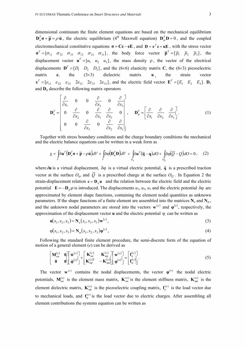
dimensional continuum the finite element equations are based on the mechanical equilibrium upσD &&ρ=+T

u , the electric equilibrium (4th Maxwell equation) 0=DDTϕ , and the coupled

electromechanical constitutive equations eECεσ −= , and κEεeD += T , with the stress vector ][ 312312332211 σσσσσσ=Tσ , the body force vector ][ 321 pppT =p , the

displacement vector ][ 321 uuuT =u , the mass density ρ , the vector of the electrical

displacements ][ 321 DDDT =D , and the (6×6) elasticity matrix C, the (6×3) piezoelectric matrix e, the (3×3) dielectric matrix κ , the strain vector

]222[ 312312332211 εεεεεε=Tε , and the electric field vector ][ 321 EEET =E . Du and Dϕ describe the following matrix operators

⎥⎥⎥⎥⎥⎥⎥

⎦

⎤

⎢⎢⎢⎢⎢⎢⎢

⎣

⎡

∂∂

∂∂

∂∂

∂∂

∂∂

∂∂

∂∂

∂∂

∂∂

=

123

312

321

000

000

000

xxx

xxx

xxxTuD , ⎥

⎦

⎤⎢⎣

⎡∂∂

∂∂

∂∂

=ϕ321 xxx

TD . (1)

Together with stress boundary conditions and the charge boundary conditions the mechanical and the electric balance equations can be written in a weak form as

( ) ( )dVdVV

TTu

V

T ∫∫ ϕδϕ+ρ−+δ=χ DDupσDu && ( ) ( )∫ ∫ =−δϕ+−δ+q QO O

T dOQQdO 0qqu , (2)

where uδ is a virtual displacement, δϕ is a virtual electric potential, q is a prescribed traction vector at the surface Oq, and Q is a prescribed charge at the surface OQ . In Equation 2 the strain-displacement relation uDε u= and the relation between the electric field and the electric potential ϕϕDE −= is introduced. The displacements u1, u2, u3 and the electric potential δϕ are approximated by element shape functions, containing the element nodal quantities as unknown parameters. If the shape functions of a finite element are assembled into the matrices Nu and Nϕ , and the unknown nodal parameters are stored into the vectors ( )ew and ( )eφ , respectively, the approximation of the displacement vector u and the electric potential ϕ can be written as

( ) ( ) ( )eu xxxxxx wNu 321321 ,,,, = , (3)

( ) ( ) ( )exxxxxx φN 321321 ,,,, ϕ=ϕ , (4)

Following the standard finite element procedure, the semi-discrete form of the equation of motion of a general element (e) can be derived as

( ) ( )

( )

( ) ( )

( ) ( )

( )

( )

( )

( )⎥⎥⎦

⎤

⎢⎢⎣

⎡=⎥

⎦

⎤⎢⎣

⎡

⎥⎥⎦

⎤

⎢⎢⎣

⎡

−+⎥

⎦

⎤⎢⎣

⎡⎥⎦

⎤⎢⎣

⎡

ϕϕϕϕ

ϕe

eu

e

eTeu

eu

euu

eeuu

ff

φw

KKKK

φw

000M

ee&&

&&. (5)

The vector )(ew contains the nodal displacements, the vector )(eφ the nodal electric potentials, )(e

uuM is the element mass matrix, )(euuK is the element stiffness matrix, )(e

ϕϕK is the

element dielectric matrix, )(euϕK is the piezoelectric coupling matrix, )(e

uf is the load vector due

to mechanical loads, and )(eϕf is the load vector due to electric charges. After assembling all

element contributions the systems equation can be written as

4 SMART’09

,⎥⎦

⎤⎢⎣

⎡=⎥

⎦

⎤⎢⎣

⎡⎥⎦

⎤⎢⎣

⎡−

+⎥⎦

⎤⎢⎣

⎡⎥⎦

⎤⎢⎣

⎡+⎥

⎦

⎤⎢⎣

⎡⎥⎦

⎤⎢⎣

⎡

ϕϕϕϕ

ϕ

ffw

KKKKw

000Cw

000M w

Tu

uuuuuuu

ϕϕϕ &

&

&&

&& (6)

where w contains the nodal mechanical degrees of freedom, ϕ the nodal electric potentials, Muu is the mass matrix, Cuu is the damping matrix, Kuu is the stiffness matrix, Kϕϕ is the dielectric matrix, Kuϕ is the piezoelectric coupling matrix, fu is the mechanical load vector, and fϕ is the electric load vector. In a compact form Equation (6) can be written as

),()( ttCEd uBfEFFFKqqDqM +=+==++ &&& (7)

where the vector q includes all nodal degrees of freedom (mechanical displacements and electric potentials). The matrices M, Dd, and K are the mass matrix, the damping matrix and the stiffness matrix, respectively. In Equation 7 the total load vector is divided into the vector f(t) of external disturbances, and the vector of the controller influence u(t); E and B describe the positions of the forces and the control parameters, respectively. This approach has been used to develop a comprehensive library of multi-field finite elements for smart structures design, which include 1D, 2D, 3D elements as well as thick and thin layered composite shell elements.

2.3 Finite element modeling of the acoustic fluid A homogeneous and inviscid acoustic fluid can be regarded as small perturbations related to an ambient reference state, which can be described by using the linear acoustic wave equation (Balachandran et al. 1996)

pc

p &&2

1=Δ , (8)

Here Δ is the Laplacian operator ][ 23

2

22

2

21

2

xxxT

∂∂

∂∂

∂∂ ++=∇∇=Δ , with ][

321 xxx ∂∂

∂∂

∂∂=∇ , p is the

acoustic pressure; and c is the sound speed. The finite element approximation of the pressure results finally in un-symmetric system matrices (Desmet & Vandepitte 1999). Everstine (1997) has recommended introducing the velocity potential Φ as a new degree of freedom in order to get symmetric matrices. The velocity potential is a scalar field which is related to the velocity v of the fluid particles by

Φ−∇= Tv , (9)

and to the sound pressure by

Φρ= &0p . (10)

After some derivation the linear wave equation, written in the velocity potential formulation, is derived (see Kollmann 2000) as

012 =∇∇− ΦΦ T

c&& . (11)

At the boundary of the fluid region the normal velocity is prescribed by nn vv = , resulting in

nn vv −=−=∂∂

nΦ (12)

With this boundary condition also the coupling with a vibrating structure can be realized. Applying the principle of virtual fluid potentials (Olson & Bathe 1985) to Equations 11 and 12, the weak form of the velocity potential formulation is derived as

∫∫ =−δ+−∇∇δ=χO

nnV

T dOvvdVc

0)()1( 2 ΦΦΦΦ && , (13)

IV ECCOMAS Thematic Conference on Smart Structures and Materials 5

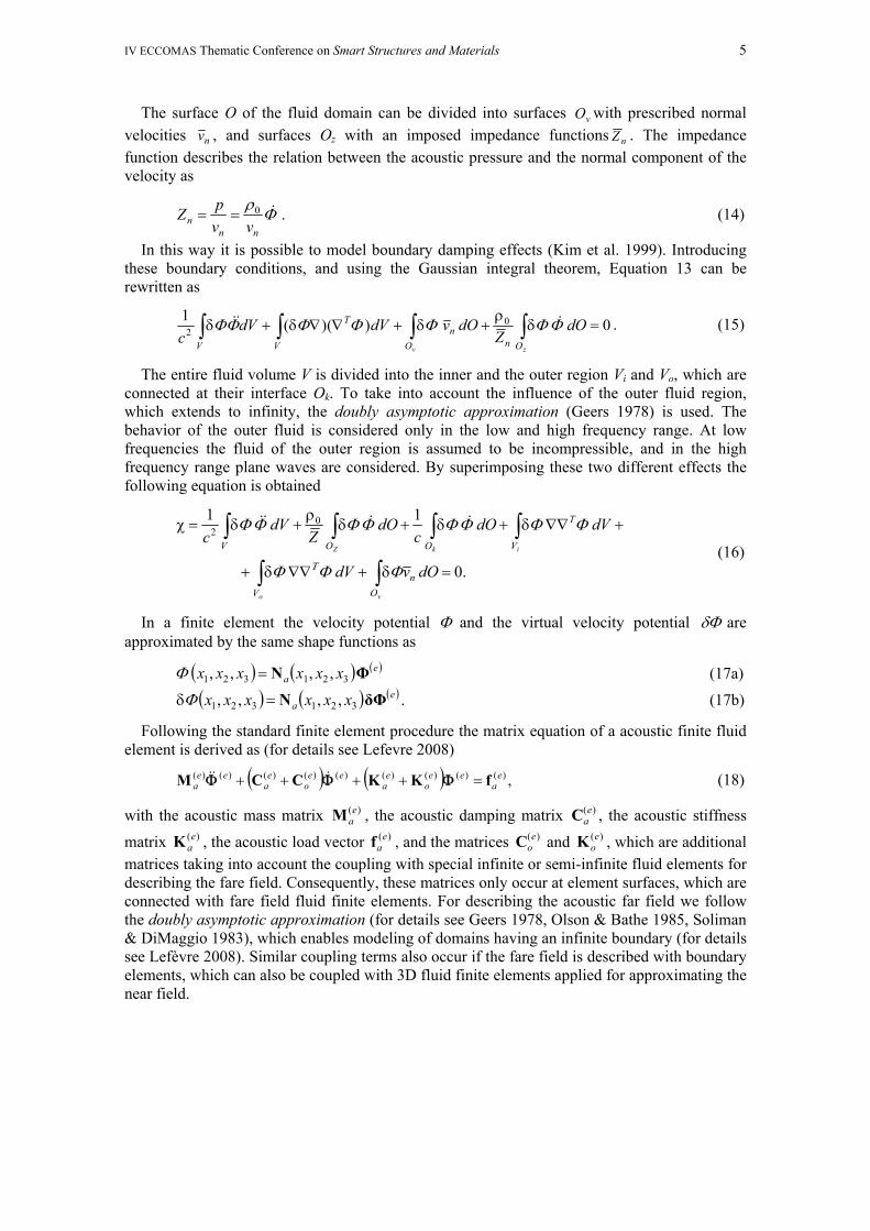
The surface O of the fluid domain can be divided into surfaces vO with prescribed normal velocities nv , and surfaces Oz with an imposed impedance functions nZ . The impedance function describes the relation between the acoustic pressure and the normal component of the velocity as

Φρ &

nnn vv

pZ 0== . (14)

In this way it is possible to model boundary damping effects (Kim et al. 1999). Introducing these boundary conditions, and using the Gaussian integral theorem, Equation 13 can be rewritten as

0)()(1 02 =δ

ρ+δ+∇∇δ+δ ∫∫∫ ∫

zv OnOn

V

T

V

dOZ

dOvdVdVc

ΦΦΦΦΦΦΦ &&& . (15)

The entire fluid volume V is divided into the inner and the outer region Vi and Vo, which are connected at their interface Ok. To take into account the influence of the outer fluid region, which extends to infinity, the doubly asymptotic approximation (Geers 1978) is used. The behavior of the outer fluid is considered only in the low and high frequency range. At low frequencies the fluid of the outer region is assumed to be incompressible, and in the high frequency range plane waves are considered. By superimposing these two different effects the following equation is obtained

.0

11 02

=δ+∇∇δ+

+∇∇δ+δ+δρ

+δ=χ

∫∫

∫∫∫∫

vo

ikZ

On

V

V

T

OOV

dOvdV

dVdOc

dOZ

dVc

ΦΦΦ

ΦΦΦΦΦΦΦΦ

Τ

&&&&

(16)

In a finite element the velocity potential Φ and the virtual velocity potential Φδ are approximated by the same shape functions as

( ) ( ) ( )ea xxxxxx ΦN 321321 ,,,, =Φ (17a)

( ) ( ) ( )ea xxxxxx δΦN 321321 ,,,, =δΦ . (17b)

Following the standard finite element procedure the matrix equation of a acoustic finite fluid element is derived as (for details see Lefevre 2008)

( ) ( ) ,)()()()()()()()()( ea

eeo

ea

eeo

ea

eea fKKCCM =++++ ΦΦΦ &&& (18)

with the acoustic mass matrix )(eaM , the acoustic damping matrix )(e

aC , the acoustic stiffness

matrix )(eaK , the acoustic load vector )(e

af , and the matrices )(eoC and )(e

oK , which are additional matrices taking into account the coupling with special infinite or semi-infinite fluid elements for describing the fare field. Consequently, these matrices only occur at element surfaces, which are connected with fare field fluid finite elements. For describing the acoustic far field we follow the doubly asymptotic approximation (for details see Geers 1978, Olson & Bathe 1985, Soliman & DiMaggio 1983), which enables modeling of domains having an infinite boundary (for details see Lefèvre 2008). Similar coupling terms also occur if the fare field is described with boundary elements, which can also be coupled with 3D fluid finite elements applied for approximating the near field.

6 SMART’09

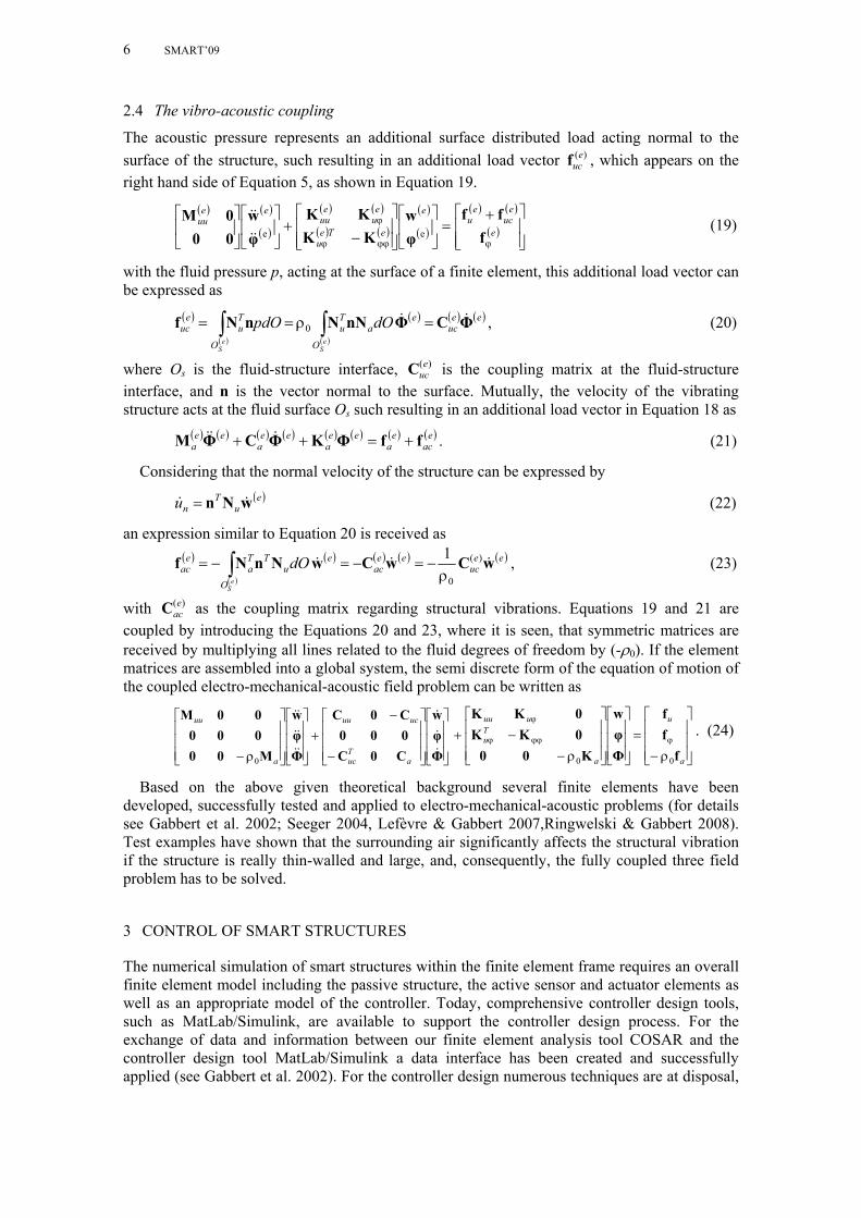
2.4 The vibro-acoustic coupling

The acoustic pressure represents an additional surface distributed load acting normal to the surface of the structure, such resulting in an additional load vector )(e

ucf , which appears on the right hand side of Equation 5, as shown in Equation 19.

( ) ( )

( )

( ) ( )

( ) ( )

( )

( )

( ) ( )

( )⎥⎥⎦

⎤

⎢⎢⎣

⎡ +=⎥

⎦

⎤⎢⎣

⎡

⎥⎥⎦

⎤

⎢⎢⎣

⎡

−+⎥

⎦

⎤⎢⎣

⎡⎥⎦

⎤⎢⎣

⎡

ϕϕϕϕ

ϕe

euc

eu

e

eTeu

eu

euu

eeuu

fff

φw

KKKK

φw

000M

ee&&

&& (19)

with the fluid pressure p, acting at the surface of a finite element, this additional load vector can be expressed as

( )

( ) ( )

( ) ( ) ( )eeuc

e

O

aTu

O

Tu

euc

eS

eS

dOpdO ΦCΦnNNnNf && =ρ== ∫∫ 0 , (20)

where Os is the fluid-structure interface, )(eucC is the coupling matrix at the fluid-structure

interface, and n is the vector normal to the surface. Mutually, the velocity of the vibrating structure acts at the fluid surface Os such resulting in an additional load vector in Equation 18 as

( ) ( ) ( ) ( ) ( ) ( ) ( ) ( )eac

ea

eea

eea

eea ffΦKΦCΦM +=++ &&& . (21)

Considering that the normal velocity of the structure can be expressed by ( )e

uT

nu wNn && = (22)

an expression similar to Equation 20 is received as ( ) ( )

( )

( ) ( ) ( )eeuc

eeac

O

eu

TTa

eac

eS

dO wCwCwNnNf &&& )(

0

1ρ

−=−=−= ∫ , (23)

with )(eacC as the coupling matrix regarding structural vibrations. Equations 19 and 21 are

coupled by introducing the Equations 20 and 23, where it is seen, that symmetric matrices are received by multiplying all lines related to the fluid degrees of freedom by (-ρ0). If the element matrices are assembled into a global system, the semi discrete form of the equation of motion of the coupled electro-mechanical-acoustic field problem can be written as

⎥⎥⎥

⎦

⎤

⎢⎢⎢

⎣

⎡

⎥⎥⎥

⎦

⎤

⎢⎢⎢

⎣

⎡

−

−+

⎥⎥⎥

⎦

⎤

⎢⎢⎢

⎣

⎡

⎥⎥⎥

⎦

⎤

⎢⎢⎢

⎣

⎡

ρ− Φφw

C0C000C0C

Φφw

M0000000M

&

&

&

&&

&&

&&

aTuc

ucuu

a

uu

0 ⎥⎥⎥

⎦

⎤

⎢⎢⎢

⎣

⎡

ρ−=

⎥⎥⎥

⎦

⎤

⎢⎢⎢

⎣

⎡

⎥⎥⎥

⎦

⎤

⎢⎢⎢

⎣

⎡

ρ−−+ ϕϕϕϕ

ϕ

a

u

a

Tu

uuu

fff

Φφw

K000KK0KK

00

. (24)

Based on the above given theoretical background several finite elements have been developed, successfully tested and applied to electro-mechanical-acoustic problems (for details see Gabbert et al. 2002; Seeger 2004, Lefèvre & Gabbert 2007,Ringwelski & Gabbert 2008). Test examples have shown that the surrounding air significantly affects the structural vibration if the structure is really thin-walled and large, and, consequently, the fully coupled three field problem has to be solved.

3 CONTROL OF SMART STRUCTURES

The numerical simulation of smart structures within the finite element frame requires an overall finite element model including the passive structure, the active sensor and actuator elements as well as an appropriate model of the controller. Today, comprehensive controller design tools, such as MatLab/Simulink, are available to support the controller design process. For the exchange of data and information between our finite element analysis tool COSAR and the controller design tool MatLab/Simulink a data interface has been created and successfully applied (see Gabbert et al. 2002). For the controller design numerous techniques are at disposal,

IV ECCOMAS Thematic Conference on Smart Structures and Materials 7

and the application of an appropriate control law is closely related to the requirements of the specific problem (see Janocha 1999, Nestorović et al. 2005-2008). For a model based controller design the large finite element models have to be reduced. One of the standard techniques is the modal reduction based on preselected eigenmodes of the system. To apply this technique, the coupled system of motion (Eq. 24) is rewritten in the following compact form.

frKrCrM ~~~~=++ &&& (25)

Introducing the state space vector

[ ] [ ]TT ΦϕΦϕ &&&& wwrrz == , (26)

from Equation 25 it follows

.~~~

~~

~~~

⎥⎦

⎤⎢⎣

⎡=+=⎥

⎦

⎤⎢⎣

⎡

−+⎥

⎦

⎤⎢⎣

⎡

0fzAzBz

M00Kz

0MMC

&& (27)

From Equation 27 the linear eigenvalue problem can be derived as

( ) 0qBA =λ− ii ˆ~~ . (28)

The solution of Equation 28 results in the modal matrix Q with 2k pairs of conjugate complex eigenvectors

[ ]k221 ˆ...ˆˆ qqqQ = . (29)

If the modal matrix Q is ortho-normalized with ( )1diag~== IQBQT and

( )iT λ== diag~

ΛQAQ , and new coordinates Qqz = are introduced in Equation 27, the reduced state space form is obtained as

⎥⎦

⎤⎢⎣

⎡=+

0fQqq~

TΛ& . (30)

If the state space Equation 30 is extended by the measurement equation the following set of equations, which can be used to design an appropriate controller, is obtained as

( ) ( )

( ) ( )tt

tt TT

EfBuAq

f0E

Qu0B

Qqq

++=

⎥⎦

⎤⎢⎣

⎡+⎥

⎦

⎤⎢⎣

⎡+−= Λ&

(31)

( ) ( ) ( )ttt FfDuCqy ++= (32)

For controller design purposes the state matrices A, B, E, C, D and F are transferred to Matlab/Simulink via the above mentioned data interface. Based on these model matrices in Matlab/Simulink different controller can be developed and tested.

4 EXPERIMENTAL VERIFICATION

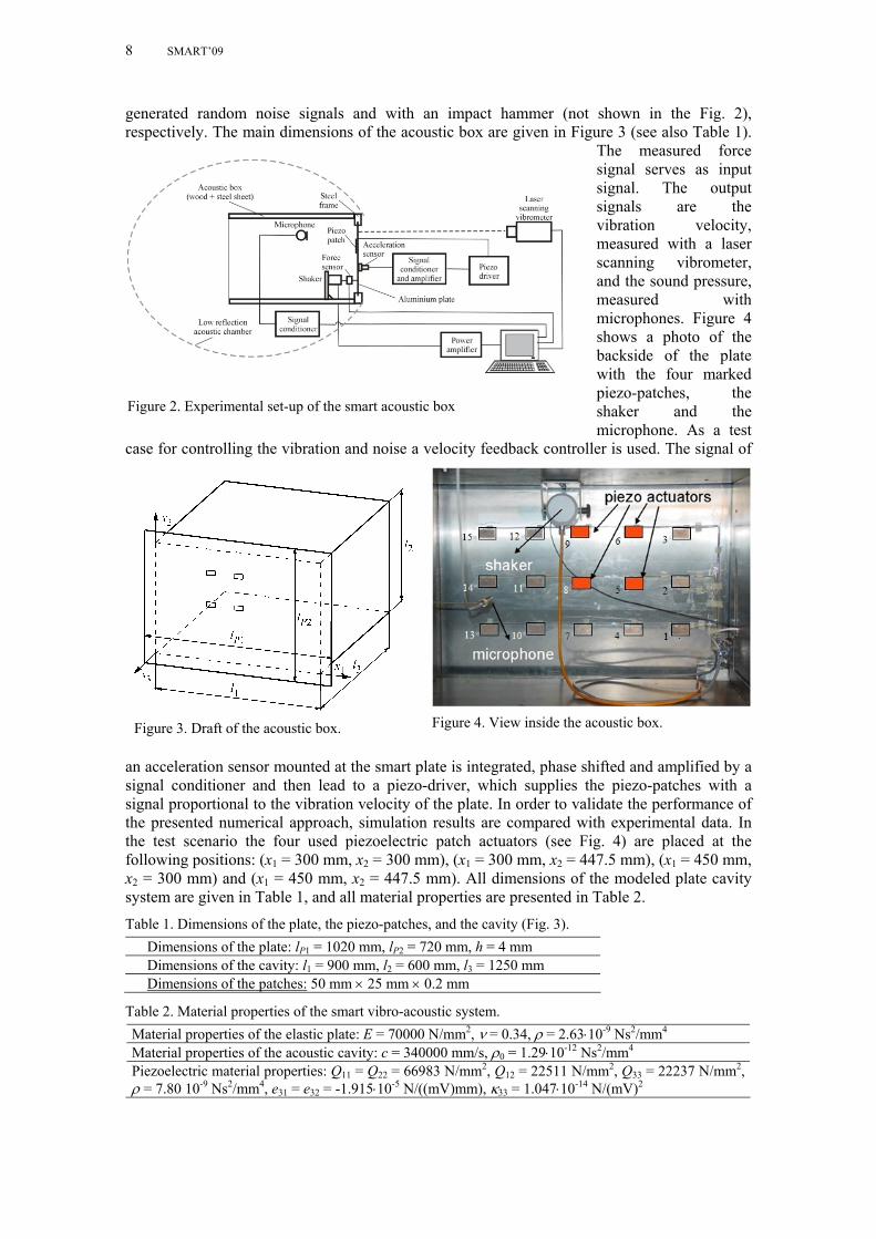
In the following as a test structure an acoustic box is presented, which is used to validate the developed numerical approach. Figure 2 shows a draft of the experimental set-up of the acoustic box with five solid side walls and an opening to the far field. Four walls are made from steel and one, the cover plate, is made from aluminium; the side opposite of the aluminium plate is open. The experiments are performed in a soundproofed room, where no fare field reflections or disturbing noise effects are influencing the experimental results. The aluminium plate is covered with piezo-electric patch actuators, four of them are used for controlling the sound pressure in the presented experiment. The aluminium plate is excited by a shaker, driven with computer

8 SMART’09

generated random noise signals and with an impact hammer (not shown in the Fig. 2), respectively. The main dimensions of the acoustic box are given in Figure 3 (see also Table 1).

The measured force signal serves as input signal. The output signals are the vibration velocity, measured with a laser scanning vibrometer, and the sound pressure, measured with microphones. Figure 4 shows a photo of the backside of the plate with the four marked piezo-patches, the shaker and the microphone. As a test

case for controlling the vibration and noise a velocity feedback controller is used. The signal of

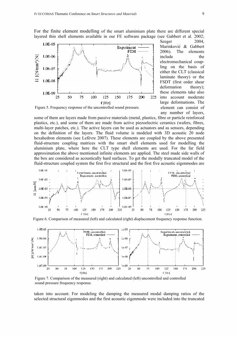
an acceleration sensor mounted at the smart plate is integrated, phase shifted and amplified by a signal conditioner and then lead to a piezo-driver, which supplies the piezo-patches with a signal proportional to the vibration velocity of the plate. In order to validate the performance of the presented numerical approach, simulation results are compared with experimental data. In the test scenario the four used piezoelectric patch actuators (see Fig. 4) are placed at the following positions: (x1 = 300 mm, x2 = 300 mm), (x1 = 300 mm, x2 = 447.5 mm), (x1 = 450 mm, x2 = 300 mm) and (x1 = 450 mm, x2 = 447.5 mm). All dimensions of the modeled plate cavity system are given in Table 1, and all material properties are presented in Table 2.

Table 1. Dimensions of the plate, the piezo-patches, and the cavity (Fig. 3). Dimensions of the plate: lP1 = 1020 mm, lP2 = 720 mm, h = 4 mm Dimensions of the cavity: l1 = 900 mm, l2 = 600 mm, l3 = 1250 mm Dimensions of the patches: 50 mm × 25 mm × 0.2 mm

Table 2. Material properties of the smart vibro-acoustic system. Material properties of the elastic plate: E = 70000 N/mm2, ν = 0.34, ρ = 2.63⋅10-9 Ns2/mm4 Material properties of the acoustic cavity: c = 340000 mm/s, ρ0 = 1.29⋅10-12 Ns2/mm4 Piezoelectric material properties: Q11 = Q22 = 66983 N/mm2, Q12 = 22511 N/mm2, Q33 = 22237 N/mm2, ρ = 7.80 10-9 Ns2/mm4, e31 = e32 = -1.915⋅10-5 N/((mV)mm), κ33 = 1.047⋅10-14 N/(mV)2

Figure 2. Experimental set-up of the smart acoustic box

Figure 3. Draft of the acoustic box. Figure 4. View inside the acoustic box.

IV ECCOMAS Thematic Conference on Smart Structures and Materials 9

For the finite element modelling of the smart aluminium plate there are different special layered thin shell elements available in our FE software package (see Gabbert et al. 2002;

Seeger 2004, Marinković & Gabbert 2006). The elements include the electromechanical coup-ling on the basis of either the CLT (classical laminate theory) or the FSDT (first order shear deformation theory); these elements take also into account moderate large deformations. The element can consist of any number of layers,

some of them are layers made from passive materials (metal, plastics, fibre or particle reinforced plastics, etc.), and some of them are made from active piezoelectric ceramics (wafers, fibres, multi-layer patches, etc.). The active layers can be used as actuators and as sensors, depending on the definition of the layers. The fluid volume is modeled with 3D acoustic 20 node hexahedron elements (see Lefèvre 2007). These elements are coupled by the above presented fluid-structure coupling matrices with the smart shell elements used for modelling the aluminium plate, where here the CLT type shell elements are used. For the far field approximation the above mentioned infinite elements are applied. The steel made side walls of the box are considered as acoustically hard surfaces. To get the modally truncated model of the fluid-structure coupled system the first five structural and the first five acoustic eigenmodes are

taken into account. For modeling the damping the measured modal damping ratios of the selected structural eigenmodes and the first acoustic eigenmode were included into the truncated

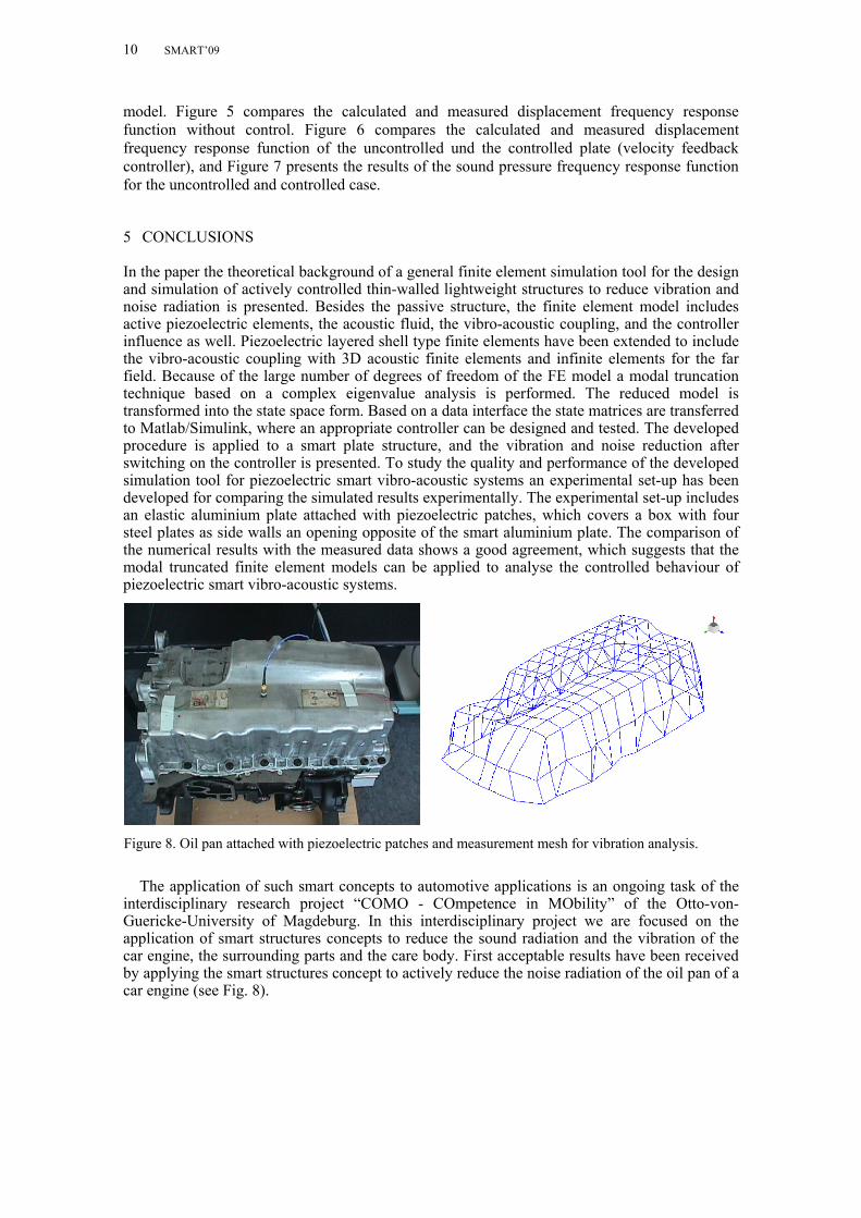
Figure 5. Frequency response of the uncontrolled sound pressure.

Figure 6. Comparison of measured (left) and calculated (right) displacement frequency response function.

Figure 7. Comparison of the measured (right) and calculated (left) uncontrolled and controlled sound pressure frequency response.

10 SMART’09

model. Figure 5 compares the calculated and measured displacement frequency response function without control. Figure 6 compares the calculated and measured displacement frequency response function of the uncontrolled und the controlled plate (velocity feedback controller), and Figure 7 presents the results of the sound pressure frequency response function for the uncontrolled and controlled case.

5 CONCLUSIONS

In the paper the theoretical background of a general finite element simulation tool for the design and simulation of actively controlled thin-walled lightweight structures to reduce vibration and noise radiation is presented. Besides the passive structure, the finite element model includes active piezoelectric elements, the acoustic fluid, the vibro-acoustic coupling, and the controller influence as well. Piezoelectric layered shell type finite elements have been extended to include the vibro-acoustic coupling with 3D acoustic finite elements and infinite elements for the far field. Because of the large number of degrees of freedom of the FE model a modal truncation technique based on a complex eigenvalue analysis is performed. The reduced model is transformed into the state space form. Based on a data interface the state matrices are transferred to Matlab/Simulink, where an appropriate controller can be designed and tested. The developed procedure is applied to a smart plate structure, and the vibration and noise reduction after switching on the controller is presented. To study the quality and performance of the developed simulation tool for piezoelectric smart vibro-acoustic systems an experimental set-up has been developed for comparing the simulated results experimentally. The experimental set-up includes an elastic aluminium plate attached with piezoelectric patches, which covers a box with four steel plates as side walls an opening opposite of the smart aluminium plate. The comparison of the numerical results with the measured data shows a good agreement, which suggests that the modal truncated finite element models can be applied to analyse the controlled behaviour of piezoelectric smart vibro-acoustic systems.

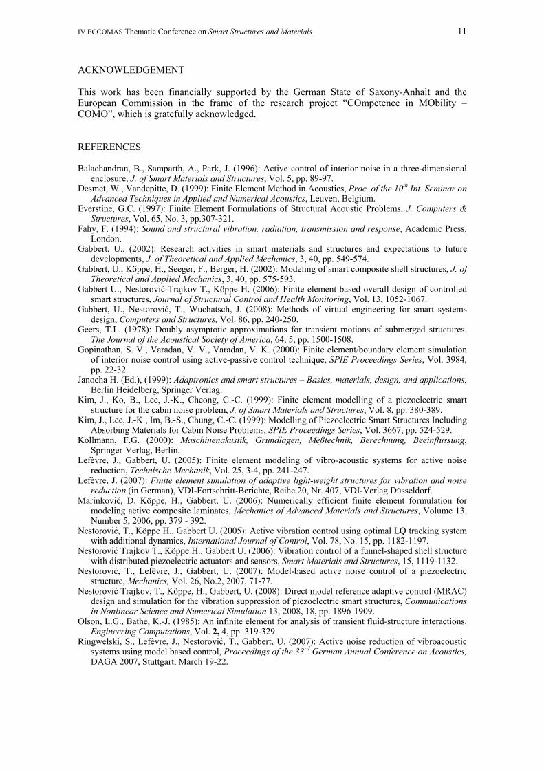
The application of such smart concepts to automotive applications is an ongoing task of the interdisciplinary research project “COMO - COmpetence in MObility” of the Otto-von-Guericke-University of Magdeburg. In this interdisciplinary project we are focused on the application of smart structures concepts to reduce the sound radiation and the vibration of the car engine, the surrounding parts and the care body. First acceptable results have been received by applying the smart structures concept to actively reduce the noise radiation of the oil pan of a car engine (see Fig. 8).

Figure 8. Oil pan attached with piezoelectric patches and measurement mesh for vibration analysis.

IV ECCOMAS Thematic Conference on Smart Structures and Materials 11

ACKNOWLEDGEMENT

This work has been financially supported by the German State of Saxony-Anhalt and the European Commission in the frame of the research project “COmpetence in MObility – COMO”, which is gratefully acknowledged.

REFERENCES

Balachandran, B., Samparth, A., Park, J. (1996): Active control of interior noise in a three-dimensional enclosure, J. of Smart Materials and Structures, Vol. 5, pp. 89-97.

Desmet, W., Vandepitte, D. (1999): Finite Element Method in Acoustics, Proc. of the 10th Int. Seminar on Advanced Techniques in Applied and Numerical Acoustics, Leuven, Belgium.

Everstine, G.C. (1997): Finite Element Formulations of Structural Acoustic Problems, J. Computers & Structures, Vol. 65, No. 3, pp.307-321.

Fahy, F. (1994): Sound and structural vibration. radiation, transmission and response, Academic Press, London.

Gabbert, U., (2002): Research activities in smart materials and structures and expectations to future developments, J. of Theoretical and Applied Mechanics, 3, 40, pp. 549-574.

Gabbert, U., Köppe, H., Seeger, F., Berger, H. (2002): Modeling of smart composite shell structures, J. of Theoretical and Applied Mechanics, 3, 40, pp. 575-593.

Gabbert U., Nestorović-Trajkov T., Köppe H. (2006): Finite element based overall design of controlled smart structures, Journal of Structural Control and Health Monitoring, Vol. 13, 1052-1067.

Gabbert, U., Nestorović, T., Wuchatsch, J. (2008): Methods of virtual engineering for smart systems design, Computers and Structures, Vol. 86, pp. 240-250.

Geers, T.L. (1978): Doubly asymptotic approximations for transient motions of submerged structures. The Journal of the Acoustical Society of America, 64, 5, pp. 1500-1508.

Gopinathan, S. V., Varadan, V. V., Varadan, V. K. (2000): Finite element/boundary element simulation of interior noise control using active-passive control technique, SPIE Proceedings Series, Vol. 3984, pp. 22-32.

Janocha H. (Ed.), (1999): Adaptronics and smart structures – Basics, materials, design, and applications, Berlin Heidelberg, Springer Verlag.

Kim, J., Ko, B., Lee, J.-K., Cheong, C.-C. (1999): Finite element modelling of a piezoelectric smart structure for the cabin noise problem, J. of Smart Materials and Structures, Vol. 8, pp. 380-389.

Kim, J., Lee, J.-K., Im, B.-S., Chung, C.-C. (1999): Modelling of Piezoelectric Smart Structures Including Absorbing Materials for Cabin Noise Problems, SPIE Proceedings Series, Vol. 3667, pp. 524-529.

Kollmann, F.G. (2000): Maschinenakustik, Grundlagen, Meßtechnik, Berechnung, Beeinflussung, Springer-Verlag, Berlin.

Lefèvre, J., Gabbert, U. (2005): Finite element modeling of vibro-acoustic systems for active noise reduction, Technische Mechanik, Vol. 25, 3-4, pp. 241-247.

Lefèvre, J. (2007): Finite element simulation of adaptive light-weight structures for vibration and noise reduction (in German), VDI-Fortschritt-Berichte, Reihe 20, Nr. 407, VDI-Verlag Düsseldorf.

Marinković, D. Köppe, H., Gabbert, U. (2006): Numerically efficient finite element formulation for modeling active composite laminates, Mechanics of Advanced Materials and Structures, Volume 13, Number 5, 2006, pp. 379 - 392.

Nestorović, T., Köppe H., Gabbert U. (2005): Active vibration control using optimal LQ tracking system with additional dynamics, International Journal of Control, Vol. 78, No. 15, pp. 1182-1197.

Nestorović Trajkov T., Köppe H., Gabbert U. (2006): Vibration control of a funnel-shaped shell structure with distributed piezoelectric actuators and sensors, Smart Materials and Structures, 15, 1119-1132.

Nestorović, T., Lefèvre, J., Gabbert, U. (2007): Model-based active noise control of a piezoelectric structure, Mechanics, Vol. 26, No.2, 2007, 71-77.

Nestorović Trajkov, T., Köppe, H., Gabbert, U. (2008): Direct model reference adaptive control (MRAC) design and simulation for the vibration suppression of piezoelectric smart structures, Communications in Nonlinear Science and Numerical Simulation 13, 2008, 18, pp. 1896-1909.

Olson, L.G., Bathe, K.-J. (1985): An infinite element for analysis of transient fluid-structure interactions. Engineering Computations, Vol. 2, 4, pp. 319-329.

Ringwelski, S., Lefèvre, J., Nestorović, T., Gabbert, U. (2007): Active noise reduction of vibroacoustic systems using model based control, Proceedings of the 33rd German Annual Conference on Acoustics, DAGA 2007, Stuttgart, March 19-22.

12 SMART’09

Ringwelski, S., Gabbert, U. (2008): Modeling and simulation of active noise and vibration control using a coupled FE-BE formulation, Proceedings of the 15th International Congress on Sound and Vibration ICSV15, pp. 1-8.

Ro, J., Baz, A., (1999): Control of sound radiation from a plate into an acoustic cavity using active constrained layer damping, J. of Smart Materials and Structures, Vol. 8, pp. 292-300.

Seeger, F., Gabbert, U., Köppe, H., Fuchs, K. (2002): Analysis and design of thin-walled smart structures in industrial applications, SPIE Proceedings Series, Vol. 4698, pp. 342-350.

Seeger, F. (2004): Simulation and optimisation of adaptive shell structures (in German), VDI-Fortschritt-Berichte, Reihe 20, VDI-Verlag GmbH Düsseldorf.

Soliman, M., DiMaggion, F.L. (1983): Doubly asymptotic approximations as non-reflecting boundaries in fluid-structure interaction problems, Computers and Structures, 17 (2), 193-204.

Tzou, H.-S., Guran, A. (Eds.), (1998): Structronic Systems: Smart Structures, Devices and Systems, Part 1: Materials and Structures, Part 2: Systems and Control, World Scientific.