Embed Size (px)
Citation preview
ACTIVE LOW-POWER MODES FOR MAIN MEMORY
BY QINGYUAN DENG
A dissertation submitted to the
Graduate School—New Brunswick
Rutgers, The State University of New Jersey
in partial fulfillment of the requirements
for the degree of
Doctor of Philosophy
Graduate Program in Computer Science
Written under the direction of
Professor Ricardo Bianchini
and approved by
New Brunswick, New Jersey
May, 2014

ABSTRACT OF THE DISSERTATION
Active Low-Power Modes for Main Memory
by Qingyuan Deng
Dissertation Director: Professor Ricardo Bianchini
Main memory is responsible for a significant fraction of the energy consumed by servers.
Prior work has focused on exploiting memory low-power states to conserve energy. How-
ever, these states require entire ranks of DRAM to be idle, which is difficult to achieve
even in lightly loaded servers. In this work, we propose three techniques for exploiting
active low-power modes to conserve full-system energy, while remaining within user-
prescribed performance bounds. The first technique, called MemScale, creates active
memory system low-power modes by applying dynamic voltage and frequency scaling
to the memory controller and dynamic frequency scaling to the memory channels and
DRAM devices. The second technique, called CoScale, coordinates the CPU and main
memory active low-power modes to avoid instability and increase energy savings. The
third technique, called MultiScale, tackles servers with multiple memory controllers,
by coordinating the active low-power modes across the controllers. Our extensive re-
sults demonstrate that the three techniques reduce full-system energy consumption
significantly, compared to prior approaches, while consistently remaining within the
user-prescribed performance bounds. We conclude that the potential benefits of those
three mechanisms and policies more than compensate for their small hardware cost.
ii
Acknowledgements
First and foremost, I would like to thank my advisor and friend Ricardo Bianchini
for his guidance and patience to me all these years, and his great character, honest,
perseverance, passion and humor. Thanks for all the days and nights working closely on
every deep details, discussions, writings, presentations, and the unforgettable overnight
deadline-run of my first paper submission. His positive attitudes to both work and life
and the pursuit of perfection will influence my career in the future. Let me also extend
the thanks to Marcia and Daniel—we always keep Ricardo in the lab too late.
I heartily thank my Ph.D. committee members Thu Nguyen, Abhishek Bhattachar-
jee and Margaret Martonosi, for all the guidances, courses, and feedbacks to the thesis.
I would like to thank my collaborators David Meisner and Thomas F. Wenisch (Univer-
sity of Michigan) too. I also would like to thank my internship mentors and colleagues
Qiang Wu, Bin Li (Facebook), Jonathan A. Winter, Taliver Heath (Google), Paul Peng
and Gansha Wu (Intel China Research Center).
Also to the Dark Lab family: we had a lot of good time working hard together,
as well as fighting hard for the milkshake. It is a great pleasure to work with my
labmates, Fabio Oliveira, Ann Paula Centeno, Wei Zheng, Rekha Bachwani, Kien Le,
Luiz Ramos, Inigo Goiri, Cheng Li, William Katsak, Guilherme Cox, Josep Lluis Berral,
Ioannis Manousakis, and Yanpei Liu. Thanks to the other colleagues, professors, staffs
in the department, and all my friends.
I would like to specially thank my wife Julia for her accompany and support all the
time. There were ups and downs through the Ph.D. years, thanks for making my life
happy and bright. Thanks to my parents, parents in-law, and the whole family for their
remote support and encouragement from China.
iii
Dedication
To my family.
iv
Table of Contents
Abstract . . . . . . . . . . . . . . . . . . . . . . . . . . . . . . . . . . . . . . . . ii
Acknowledgements . . . . . . . . . . . . . . . . . . . . . . . . . . . . . . . . . iii
Dedication . . . . . . . . . . . . . . . . . . . . . . . . . . . . . . . . . . . . . . . iv
List of Tables . . . . . . . . . . . . . . . . . . . . . . . . . . . . . . . . . . . . . viii
List of Figures . . . . . . . . . . . . . . . . . . . . . . . . . . . . . . . . . . . . ix
1. Introduction . . . . . . . . . . . . . . . . . . . . . . . . . . . . . . . . . . . 1
1.1. In This Dissertation . . . . . . . . . . . . . . . . . . . . . . . . . . . . . 3
1.1.1. MemScale . . . . . . . . . . . . . . . . . . . . . . . . . . . . . . . 3
1.1.2. CoScale . . . . . . . . . . . . . . . . . . . . . . . . . . . . . . . . 4
1.1.3. MultiScale . . . . . . . . . . . . . . . . . . . . . . . . . . . . . . . 4
1.2. Contributions . . . . . . . . . . . . . . . . . . . . . . . . . . . . . . . . . 5
1.3. Dissertation Structure . . . . . . . . . . . . . . . . . . . . . . . . . . . . 6
2. Background . . . . . . . . . . . . . . . . . . . . . . . . . . . . . . . . . . . . 7
2.1. Server Power Management . . . . . . . . . . . . . . . . . . . . . . . . . . 7
2.2. Memory System Technology . . . . . . . . . . . . . . . . . . . . . . . . . 11
2.3. Impact of Memory Voltage and Frequency Scaling . . . . . . . . . . . . 14
2.4. Conclusion . . . . . . . . . . . . . . . . . . . . . . . . . . . . . . . . . . 15
3. MemScale . . . . . . . . . . . . . . . . . . . . . . . . . . . . . . . . . . . . . 17
3.1. Introduction . . . . . . . . . . . . . . . . . . . . . . . . . . . . . . . . . . 17
3.2. MemScale Design . . . . . . . . . . . . . . . . . . . . . . . . . . . . . . . 19
3.2.1. Hardware and Software Mechanisms . . . . . . . . . . . . . . . . 19
v
3.2.2. Energy Management Policy . . . . . . . . . . . . . . . . . . . . . 22
3.2.3. Performance and Energy Models . . . . . . . . . . . . . . . . . . 25
3.2.4. Hardware and Software Costs . . . . . . . . . . . . . . . . . . . . 30
3.3. Evaluation . . . . . . . . . . . . . . . . . . . . . . . . . . . . . . . . . . . 31
3.3.1. Methodology . . . . . . . . . . . . . . . . . . . . . . . . . . . . . 31
3.3.2. Results . . . . . . . . . . . . . . . . . . . . . . . . . . . . . . . . 35
3.4. Conclusion . . . . . . . . . . . . . . . . . . . . . . . . . . . . . . . . . . 46
4. CoScale . . . . . . . . . . . . . . . . . . . . . . . . . . . . . . . . . . . . . . 47
4.1. Introduction . . . . . . . . . . . . . . . . . . . . . . . . . . . . . . . . . . 47
4.2. CoScale Design . . . . . . . . . . . . . . . . . . . . . . . . . . . . . . . . 49
4.2.1. CoScale’s Frequency Selection Algorithm . . . . . . . . . . . . . 52
4.2.2. Comparison with Other Policies . . . . . . . . . . . . . . . . . . 55
4.2.3. Implementation . . . . . . . . . . . . . . . . . . . . . . . . . . . . 58
4.2.4. Hardware and Software Costs . . . . . . . . . . . . . . . . . . . . 61
4.3. Evaluation . . . . . . . . . . . . . . . . . . . . . . . . . . . . . . . . . . . 62
4.3.1. Methodology . . . . . . . . . . . . . . . . . . . . . . . . . . . . . 62
4.3.2. Results . . . . . . . . . . . . . . . . . . . . . . . . . . . . . . . . 64
4.4. Conclusion . . . . . . . . . . . . . . . . . . . . . . . . . . . . . . . . . . 74
5. MultiScale . . . . . . . . . . . . . . . . . . . . . . . . . . . . . . . . . . . . . 75
5.1. Introduction . . . . . . . . . . . . . . . . . . . . . . . . . . . . . . . . . . 75
5.2. Motivation . . . . . . . . . . . . . . . . . . . . . . . . . . . . . . . . . . 77
5.3. MultiScale Design . . . . . . . . . . . . . . . . . . . . . . . . . . . . . . 78
5.3.1. Hardware and Software . . . . . . . . . . . . . . . . . . . . . . . 79
5.3.2. Performance and Energy Models . . . . . . . . . . . . . . . . . . 80
5.4. Evaluation . . . . . . . . . . . . . . . . . . . . . . . . . . . . . . . . . . . 83
5.4.1. Methodology . . . . . . . . . . . . . . . . . . . . . . . . . . . . . 83
5.4.2. Results . . . . . . . . . . . . . . . . . . . . . . . . . . . . . . . . 85
5.5. Conclusion . . . . . . . . . . . . . . . . . . . . . . . . . . . . . . . . . . 87
vi

6. Related Work . . . . . . . . . . . . . . . . . . . . . . . . . . . . . . . . . . . 88
7. Conclusion and Future Work . . . . . . . . . . . . . . . . . . . . . . . . . 93
7.1. Future work . . . . . . . . . . . . . . . . . . . . . . . . . . . . . . . . . . 94
References . . . . . . . . . . . . . . . . . . . . . . . . . . . . . . . . . . . . . . . 96
vii

List of Tables
3.1. MemScale workload descriptions. . . . . . . . . . . . . . . . . . . . 32
3.2. MemScale simulation parameters. . . . . . . . . . . . . . . . . . . . 33
4.1. CoScale workload descriptions. . . . . . . . . . . . . . . . . . . . . . 63
5.1. MultiScale workload descriptions. . . . . . . . . . . . . . . . . . . . 84
viii

List of Figures
2.1. ACPI global and processor low-power states. . . . . . . . . . . . . 8
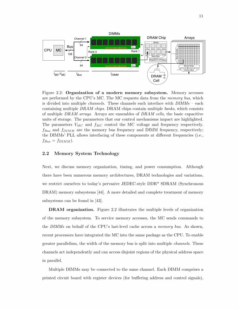
2.2. Organization of a modern memory subsystem. Memory accesses
are performed by the CPU’s MC. The MC requests data from the mem-
ory bus, which is divided into multiple channels. These channels each
interface with DIMMs – each containing multiple DRAM chips. DRAM
chips contain multiple banks, which consists of multiple DRAM arrays.
Arrays are ensembles of DRAM cells, the basic capacitive units of storage.
The parameters that our control mechanisms impact are highlighted.
The parameters VMC and fMC control the MC voltage and frequency re-
spectively. fBus and fDIMM are the memory bus frequency and DIMM
frequency, respectively; the DIMMs’ PLL allows interfacing of these com-
ponents at different frequencies (i.e., fBus = fDIMM ). . . . . . . . . . . 11
2.3. Conventional memory subsystem power breakdown. There is
substantial opportunity for memory active low-power modes: it can re-
duce Background, PLL/REG, and MC power. . . . . . . . . . . . . . . . 13
3.1. Memscale operation: In this example, we illustrate the operation of
MemScale for two cores. The best-case execution time is calculated at
each epoch (“Max Frequency”). The target time is a fixed percent slower
than this best case. Slack is the time difference between the target and
current execution; it is accumulated across epochs. Note that since the
frequency transition time, Ttr, is so small compared to the epoch, the
performance penalty is insignificant. . . . . . . . . . . . . . . . . . . . . 25
ix

3.2. Memory subsystem queuing model: Banks and channels are repre-
sented as servers. The cores issue requests to bank servers, which proceed
to the channel server upon completion. Because of DRAM operation, re-
quests are held at the bank server until a request frees from the channel
server (the channel server has a queue depth of 0). In our example,
the request that finishes at bank 1 cannot proceed to the bus until the
request already there leaves. This example shows only a single channel. 28
3.3. Energy savings. Memory and full-system energies are significantly
reduced, particularly for the ILP workloads. . . . . . . . . . . . . . . . . 36
3.4. CPI overhead. Both average and worst-case CPI overheads fall well
within the target degradation bound. . . . . . . . . . . . . . . . . . . . 37
3.5. Timeline of MID3 workload in MemScale MemScale adjusts mem-
ory system frequency rapidly in response to the phase change in apsi. . 38
3.6. Timeline of MEM4 workload in MemScale. MemScale approxi-
mates a “virtual frequency” by oscillating between two neighboring fre-
quencies. . . . . . . . . . . . . . . . . . . . . . . . . . . . . . . . . . . . . 38
3.7. Energy savings. MemScale provides greater full-system and memory
system energy savings than alternatives. . . . . . . . . . . . . . . . . . . 40
3.8. System energy breakdown. MemScale reduces DRAM, PLL/Reg,
and MC energy more than alternatives. . . . . . . . . . . . . . . . . . . 40
3.9. CPI overhead. MemScale’s CPI increases are under 10%. MemScale
(MemEnergy) slightly exceeds the bound. . . . . . . . . . . . . . . . . . 40
3.10. Impact of CPI bound. Increasing the bound beyond 10% does not
yield further energy savings. . . . . . . . . . . . . . . . . . . . . . . . . . 43
3.11. Impact of number of channels. MemScale provides greater savings
when there are more, less-utilized channels. . . . . . . . . . . . . . . . . 44
3.12. Impact of fraction of memory power. Increasing the fraction in-
creases energy savings. . . . . . . . . . . . . . . . . . . . . . . . . . . . . 44
x

3.13. Impact of power proportionality of MC and registers. Decreasing
proportionality increases energy savings. . . . . . . . . . . . . . . . . . . 45
4.1. CoScale operation: Semi-coordinated oscillates, whereas CoScale scales
frequencies more accurately. . . . . . . . . . . . . . . . . . . . . . . . . . 52
4.2. CoScale’s greedy gradient-descent frequency selection algorithm. 54
4.3. Sub-algorithm to consider core frequency changes by group. . . 54
4.4. Search differences: CoScale searches the parameter space efficiently. Unco-
ordinated violates the performance bound and Semi-coordinated gets stuck in
local minima. . . . . . . . . . . . . . . . . . . . . . . . . . . . . . . . . . . 57
4.5. CoScale energy savings. CoScale conserves up to 24% of the full-system
energy. . . . . . . . . . . . . . . . . . . . . . . . . . . . . . . . . . . . . . 65
4.6. CoScale performance. CoScale never violates the 10% performance bound. . 65
4.7. Timeline of the milc application in MIX2. Milc exhibits three phases.
CoScale adjusts core and memory subsystem frequency precisely and rapidly in
response to the phase changes. The other techniques do not. . . . . . . . . . 66
4.8. Energy savings. CoScale provides greater full-system energy savings
than the practical policies. . . . . . . . . . . . . . . . . . . . . . . . . . 68
4.9. Performance. Uncoordinated is incapable of limiting performance degra-
dation. . . . . . . . . . . . . . . . . . . . . . . . . . . . . . . . . . . . . . 69
4.10. Impact of performance bound. Higher bound allows more savings
without violations. . . . . . . . . . . . . . . . . . . . . . . . . . . . . . . 70
4.11. Impact of rest-of-system power. Savings still high for higher rest-
of-system power. . . . . . . . . . . . . . . . . . . . . . . . . . . . . . . . 70
4.12. Impact of CPU:mem power, MID. Savings increase as memory
power increases. . . . . . . . . . . . . . . . . . . . . . . . . . . . . . . . . 70
4.13. Impact of CPU:mem power, MEM. Savings decrease as memory
power increases. . . . . . . . . . . . . . . . . . . . . . . . . . . . . . . . . 70
4.14. Impact of CPU voltage range. Smaller voltage ranges reduce energy
savings. . . . . . . . . . . . . . . . . . . . . . . . . . . . . . . . . . . . . 71
xi

4.15. Impact of number of frequencies. Savings decrease little when fewer
steps are avalaible. . . . . . . . . . . . . . . . . . . . . . . . . . . . . . . 71
4.16. Impact of prefetching. CoScale works well with and without prefetching. 71
4.17. In-order vs OoO: performance. CoScale is within the performance
bound in both in-order and OoO. . . . . . . . . . . . . . . . . . . . . . . 73
4.18. In-order vs OoO: energy. CoScale saves similar percent of energy in
in-order and OoO. . . . . . . . . . . . . . . . . . . . . . . . . . . . . . . 73
5.1. Because it independently manages each MC, MultiScale can se-
lect a lower frequency for MC 0 and thus save more energy than
MemScale while remaining within the prescribed performance
bounds. . . . . . . . . . . . . . . . . . . . . . . . . . . . . . . . . . . . . 77
5.2. (a) MultiScale’s energy savings assuming that 80% of an appli-
cation’s pages are mapped to its local MC and a 10% perfor-
mance loss bound; (b) MultiScale’s actual performance loss in
this scenario. . . . . . . . . . . . . . . . . . . . . . . . . . . . . . . . . 85
5.3. MultiScale’s energy savings versus MemScale across a spectrum
of traffic skews and performance degradation bounds. MultiScale consis-
tently provides greater energy savings than MemScale. . . . . . . . . . 86
5.4. MultiScale’s worst performance degradation versus MemScale
across a spectrum of traffic skews and performance degradation bounds.
MultiScale leads to slightly higher degradations than MemScale. . . . . 87
xii

1
Chapter 1
Introduction
Over the last 10 years, it has become clear that the massive energy consumption
of datacenters represents a serious burden on their operators and on the environment
[23]. Concern over energy waste has led to numerous academic (e.g., [67, 72, 77]) and
industrial efforts to improve the efficiency of datacenter infrastructure. Although the
datacenters’ power delivery and cooling systems respond for a non-trivial fraction of
this energy, the largest fraction by far (roughly 90% at an aggressive Power Utilization
Efficiency of 1.07) is due to the servers themselves [28, 71].
Within the server, the processor has dominated energy consumption. However, as
processors have become more energy-efficient and more effective at managing their own
power consumption, they are more energy proportional. In contrast, in most servers
main memory consumes the second largest fraction of the total energy consumption,
and it is less energy proportional [8, 51, 57, 86], as multi-core servers are requiring
increasing main memory bandwidth and capacity. Making matters worse, memory
energy management is challenging in the context of servers with modern (DDR*1)
DRAM technologies. Today, main memory accounts for a range between 10% to 40%
of server energy [8, 86]—only lower than the processors’ contribution. In reality, the
fraction attributable to memory accesses may be even higher, since these estimates do
not consider the memory controller’s energy consumption.
The early works on memory energy conservation focused on creating memory idle-
ness through scheduling, batching, layout transformations, and architecture modifica-
tion so that idle low-power states could be exploited [21, 24, 37, 48, 56, 70, 60]. Those
studies generally assumed the rich, chip-level power management permitted in older
1DDR* refers to the family of Double Data Rate memory devices.

2
technologies, such as RDRAM [17]. Another category of works have considered reduc-
ing the number of DRAM chips that are accessed at a time (rank subsetting) [3, 90]
and even changing the microarchitecture of the DRAM chips themselves to improve
energy efficiency [16, 84]. A common theme of these works is to reduce the number
of chips or bits actually touched as a result of a memory access, thereby reducing the
dynamic memory energy consumption. More recent works have studied alternative
memory technologies to replace traditional DRAM modules, such as Mobile DRAM
and PCM [34, 59].
We argue that none of these approaches is ideal. Rank subsetting requires changes
to the architecture of the memory DIMMs (Dual In-Line Memory Modules), which
are expensive and increase latency. Changing DRAM chip microarchitecture may have
negative implications on capacity and yield. Using mobile memory technology sacrifices
performance and reliability, while new memory technologies are not yet widely avail-
able. Idle low-power states rely on server idleness. Although in many scenarios servers
are underutilized, they are rarely completely idle [8]. Creating enough idleness is dif-
ficult in modern DDR* memories, since power management is available only at coarse
granularity (entire ranks spanning multiple chips). Thus, deep idle low-power states
can rarely be used without excessively degrading performance. For this reason, today,
even the most aggressive memory controllers use only shallow, fast-exit power-down
states to conserve energy while idle.
Compared to idle low-power states, active low-power modes are more appropriate
for today’s server workload while not requiring full idleness. They can save energy
during low system utilization with much smaller performance cost. For example, Google
reports that the server idle periods in its search workload are no longer than a few
milliseconds [8]. Such short idle periods preclude the use of deep idle low-power states
and limit energy savings [62]. On the other hand, in high CPU utilization scenarios, such
as HPC workloads, peak memory bandwidth is not always needed. Active low-power
modes may still be applied to conserve energy if they do not excessively increase memory
latency. Traditionally, the CPU has exposed active low-power modes via Dynamic
Voltage and Frequency Scaling (DVFS). Under those modes, instructions still execute

3
but at a lower rate. Researchers have considered active low-power modes for disks
[14, 33] and network interfaces [31, 69]. In this dissertation, we propose active low-
power modes for the main memory subsystem as well.
1.1 In This Dissertation
In this dissertation, we propose to create active low-power modes for the main memory
subsystem, as well as three techniques for transitioning between those modes. The
techniques seek to conserve full-system energy, while remaining within user-prescribed
performance bounds.
1.1.1 MemScale
The first technique, called MemScale, creates a set of active low-power modes, hardware
mechanisms, and software policies to conserve energy while respecting the applications’
performance requirements. Specifically, MemScale creates and leverages active low-
power modes for the main memory subsystem (formed by the memory devices and the
memory controller). Our approach is based on the key observation that server work-
loads, though often highly sensitive to memory access latency, only rarely demand peak
memory bandwidth. To exploit this observation, we propose to apply DVFS to the
memory controller and Dynamic Frequency Scaling (DFS) to the memory channels and
DRAM devices. By dynamically varying voltages and frequencies, our policies trade
available memory bandwidth to conserve energy when memory activity is low. Although
lowering voltage and frequency causes increases in channel transfer time, controller la-
tency, and queueing time at the controller, other components of the memory access
latency are essentially not affected. As a result, these overheads have only a minor
impact on average latency. Also importantly, MemScale requires only limited hardware
changes—none involving the DIMMs or DRAM chips—since most of the required mech-
anisms are already present in current memory systems. In fact, many servers already
allow one of a small number of memory channel frequencies to be statically selected at
boot time. Our results demonstrate that MemScale can conserve significant full-system

4
energy within user-defined maximum acceptable performance degradation.
1.1.2 CoScale
The second technique, called CoScale, further coordinates main memory active low-
power modes with CPU active low-power modes to avoid instability and increase en-
ergy savings. We find that simply supporting separate processor and memory active
low-power modes is insufficient, as independent control policies often conflict, leading
to oscillations, unstable behavior, or sub-optimal power/performance trade-offs. To
accomplish this coordinated control, we rely on execution profiling of core and memory
access performance, using existing and new performance counters. Through counter
readings and analytic models of core and memory performance and power consump-
tion, we assess opportunities for per-core voltage and frequency scaling in a chip mul-
tiprocessor, voltage and frequency scaling of the on-chip memory controller (MC), and
frequency scaling of memory channels and DRAM devices. The fundamental innova-
tion of CoScale is the way it efficiently searches the space of per-core and memory
frequency settings (we set voltages according to the selected frequencies) in software.
Essentially, our epoch-based policy estimates, via our performance counters and online
models, the energy and performance cost/benefit of altering each component’s (or set
of components’) DVFS state by one step, and iterates to greedily select a new frequency
combination for cores and memory. Our results demonstrate that CoScale conserves
significantly more full-system energy than policies that control only the CPU power
modes or only the memory power modes. CoScale also behaves better than policies
that independently control both resources.
1.1.3 MultiScale
The third technique, called MultiScale, tackles servers with multiple MCs, by coor-
dinating the active low-power modes across the controllers. Recent hardware trends
suggest that traffic skew across MCs will grow. For example, as servers increasingly
rely on multi-socket configurations, inter-socket MC bandwidth requirements will vary
significantly [86]. In addition, the advent of heterogeneous processors incorporating

5
sophisticated superscalar out-of-order cores with simpler in-order cores (e.g., ARM’s
big.LITTLE architecture [30]), and graphics processing units (e.g., AMD’s Fusion and
Intel’s Sandybridge architectures [79]), will fundamentally increase traffic skew across
MCs. Therefore, it is critical to explore techniques for managing active low-power
modes in the presence of multiple MCs. MultiScale monitors per-application traffic
across MCs and estimates their varying bandwidth and latency requirements. It then
uses a heuristic algorithm to quickly select and apply an optimized per-MC frequency
combination. Our results show that MultiScale is particularly effective in scenarios
where traffic is skewed across MCs and when the allowable performance degradation is
low.
1.2 Contributions
In summary, our contributions in this dissertation are:
• We propose MemScale, a technique that creates active low-power modes for the
main memory system by applying DFS / DVFS to memory channels, DIMMs,
and memory controllers;
• We evaluate MemScale for a large set of multiprogrammed workloads. Our evalu-
ation compares MemScale to the state-of-the-art in memory energy management;
• We propose CoScale, a coordinated approach for CPU and memory DVFS. CoScale
embodies an efficient algorithm for searching the space of per-core and memory
frequency settings;
• We also evaluate CoScale for a large set of multiprogrammed workloads. We
compare it to DVFS policies that only control a single resource, and policies that
independently control both resources;
• We propose MultiScale, an approach to coordinate active low-power modes among
multiple memory controllers;
• We evaluate MultiScale for a large set of multiprogrammed workloads with a wide
range of memory traffic patterns;

6
• Among MemScale, CoScale, and MultiScale, we propose multiple new hardware
performance counters to enable better workload profiling and modeling.
1.3 Dissertation Structure
The remainder of this dissertation is organized as follows. Chapter 2 provides an
overview of existing server power management techniques, the main memory system,
and the impact of active low-power modes on energy and performance. In Chapter 3,
we detail the design and evaluation of MemScale. In Chapter 4, we present the details
and evaluation of CoScale. Chapter 5 discusses the design and evaluation of MultiScale.
In Chapter 6, we discuss the related work. Chapter 7 concludes the dissertation and
discusses the future work.

7
Chapter 2
Background
In this chapter, we provide a brief overview of server power states, modern memory
subsystems, and the impact of DFS / DVFS on memory systems’ performance and
power consumption.
2.1 Server Power Management
Modern servers already support many idle and active low-power states both at the
component and server levels. The Advanced Configuration and Power Interface (ACPI)
specification [2] defines the open standards for server power management. It provides
platform-independent interfaces in the hardware and firmware to enable the Operating
System (OS) to control the transitions among states.
Global power states. As shown in Figure 2.1, according to ACPI, there are four
global states: G0 to G3. G0 (also known as S0) is the working state. In G0, the server
is running and the processor is powered on—it can be either in active low-power modes
or any of the standby C states (discussed later in this section); other server components
are fully running as well in this state.
G1 state is the sleeping state. It can be further divided into four states: S1 to S4. In
S1 all the processor caches are flushed, and the processor stops executing instructions.
Both the processor and main memory are still powered on. S2 and S3 are called
“standby” states. They are similar in that, in these states, the processor is powered
off while all the contexts and dirty cache bits are saved in the memory system, which
is still powered on. S4 is the “hibernate” state, where both the processor and memory
are powered off. In this state, the processor contexts and memory contents are stored
on the disk. Although the disk is powered off, the data is retained because of the disk’s

8
Figure 2.1: ACPI global and processor low-power states.
non-volatile nature. All the data will be restored to the main memory and processor
upon the system’s return to G0 (S0).
G2 (also noted as S5) is the soft power-off state. In this state, the server is totally
powered off except the bare minimum power provided to the motherboard interface by
the power supply unit (PSU), so that the server can wake up over the LAN or from
other devices. No previous contents are retained in this state so a full system reboot is
required.
The last one is the G3 state, the mechanical power-off state. In this state the server is
completely shut down—no outside power sources are connected, only the motherboard’s
own battery may still be attached.
Processor idle/active power states. While G states are the server-level power
states, there are component-level power states too. In the G0 (S0) state, the processor
has several idle power states (named C states), and active performance states (P states
and T states). C0 is the processor’s working state. In this state, the processor usually

9
has multiple P states which expose different performance. There are many implemen-
tations of P states. Examples include Intel’s SpeedStep [40] and AMD’s Cool’n’Quiet
[5]. The P states usually leverage processor DVFS or DFS, on one or multiple processor
cores and the cache system. According to the ACPI standard, P0 consumes the max-
imum power and provides the best performance; P1’s performance is less than P0 but
consumes less power; so on and so forth. Transitions among different P states usually
take several tens of microseconds [40], depending on the voltage transition gap—voltage
can only be scaled up/down gradually.
The ACPI specification also defines T states for the processor, known as the throt-
tling states. T states apply clock gating on the processor and were originally used for
thermal management. The higher the temperature, the higher the T states, the larger
fraction of time the processor’s clock is gated. T states have been deprecated in the
modern processors.
C1 is the processor’s halt state, in which it stops executing instructions. There is also
an enhanced C1 state, named C1E, in which the processor’s frequencies and voltages
are also scaled down to their lowest levels. Therefore, in the C1E state, the processor’s
power consumption is further reduced. In the C1/C1E state, the processor’s cache
content is still retained. The processor can return to the C0 state from the C1/C1E
state essentially instantaneously (may need some time to ramp up the frequency and
voltage from the C1E state).
In the C2 and C3 states, the processor’s clocks are shut off; in the C2 state the
cache content is retained while in the C3 state, each core flushes their private cache
content into the shared L3 cache. Because the clocks are shut off, and the private cache
content is flushed, it takes much longer time to return to C0 from C2 and C3.
Some processors have even deeper C states. For example, Intel implements the C6
and C7 states in server processors [40]. In the C6 state, the processor execution cores
enter the C3 state, save their architectural contexts before removing the core voltage.
While in the C7 state, if all execution cores enter the C6 state, the shared L3 cache
will be flushed, and the voltage of the L3 cache will also be removed. The deeper the C
states, the lower the processor power consumption, and the longer it will take to restore

10
the processor back to the C0 state.
Device low-power states. ACPI defines low-power states for devices as well—D
states: D0 to D3. Similar to G0, D0 is the full operating state which provides the best
performance and consumes the highest power. D1 and D2 are intermediate low-power
states. D3 is the power off state.
Power and performance implications of ACPI states. Obviously, in active
low-power states, servers consume more power than in idle low-power states. The G0
state has the highest power consumption while the G2/G3 state essentially does not
consume any power. The power consumption of the G1 state is in between. Among
all the sleeping states, the S4 state consumes the least power—almost the same power
as G2, except that it can restore to G0 much faster (depending on how much memory
content needs to be restored). It usually takes tens of seconds to load the processor
contexts and memory content back from the disk. A full system reboot can take a
couple of minutes to transition the state from G2/G3 back to G0. The restoring time
from S3 is usually around a couple of seconds—an order of magnitude faster than the
restoring time of S4. A server in the S3 state usually consumes less than 10 watts [61].
However, all the above idle low-power states do not quite match today’s server work-
loads, which rarely expose idle periods longer than several milliseconds [8]. The active
low-power states are more appropriate. Modern servers can transition between differ-
ent P states within tens of microseconds. At different P states the processor is running
at different frequencies. The impact of P states on the server’s overall performance
depends on the characteristics of the workload. Compute-intensive workloads are more
sensitive to the processors’ frequencies than memory- or I/O-intensive workloads. Fi-
nally, in different P states, the processors’ power consumption scales more than linearly
with frequency, because of voltage scaling. However, P states only affect the power
consumption of the CPU, while the power consumption from other components in the
server is not impacted directly.
11
BusCPU MC
Channel 1
Channel 2
64
64
128
Row
Dec
oder
Sense Amps
Column Mux
DIMMsDRAM Chip Arrays
Bank Mux
Banks
Rank 0 Rank 1
fMC,VMC fBus fDIMM
DLLRegisters & I/O
PLL
DRAM Cell
PLL
Figure 2.2: Organization of a modern memory subsystem. Memory accessesare performed by the CPU’s MC. The MC requests data from the memory bus, whichis divided into multiple channels. These channels each interface with DIMMs – eachcontaining multiple DRAM chips. DRAM chips contain multiple banks, which consistsof multiple DRAM arrays. Arrays are ensembles of DRAM cells, the basic capacitiveunits of storage. The parameters that our control mechanisms impact are highlighted.The parameters VMC and fMC control the MC voltage and frequency respectively.fBus and fDIMM are the memory bus frequency and DIMM frequency, respectively;the DIMMs’ PLL allows interfacing of these components at different frequencies (i.e.,fBus = fDIMM ).
2.2 Memory System Technology
Next, we discuss memory organization, timing, and power consumption. Although
there have been numerous memory architectures, DRAM technologies and variations,
we restrict ourselves to today’s pervasive JEDEC-style DDR* SDRAM (Synchronous
DRAM) memory subsystems [44]. A more detailed and complete treatment of memory
subsystems can be found in [43].
DRAM organization. Figure 2.2 illustrates the multiple levels of organization
of the memory subsystem. To service memory accesses, the MC sends commands to
the DIMMs on behalf of the CPU’s last-level cache across a memory bus. As shown,
recent processors have integrated the MC into the same package as the CPU. To enable
greater parallelism, the width of the memory bus is split into multiple channels. These
channels act independently and can access disjoint regions of the physical address space
in parallel.
Multiple DIMMs may be connected to the same channel. Each DIMM comprises a
printed circuit board with register devices (for buffering address and control signals),

12
a Phase Lock Loop device (for maintaining frequency and phase synchronization), and
multiple DRAM chips (for data storage). The DRAM chips are the ultimate destination
of the MC commands. The subset of DRAM chips that participate in each access is
called a rank. The number of chips in a rank depends on how many bits each chip
produces/consumes at a time. For example, the size of the rank is 8 DRAM chips (or 9
chips for DIMMs with ECC) when each chip is x8 (pronounced “by 8”), since memory
channels are 64 bits wide (or 72 bits wide with ECC). Each DIMM can have up to 16
chips (or 18 chips with ECC), organized into 1-4 ranks.
Each DRAM chip contains multiple banks (typically 8 banks nowadays), each of
which contains multiple two-dimensional memory arrays. The basic unit of storage
in an array is a simple capacitor representing a bit—the DRAM cell. Thus, in a x8
DRAM chip, each bank has 8 arrays, each of which produces/consumes one bit at a
time. However, each time an array is accessed, an entire multi-KB row is transferred
to a row buffer. This operation is called an “activation” or a “row opening”. Then,
any column of the row can be read/written over the channel in one burst. Because the
activation is destructive, the corresponding row eventually needs to be “pre-charged”,
that is, written back to the array. Under a closed-page management scheme, the MC
pre-charges a row after every column access, unless there is another pending access
for the same row. Prior studies suggest that closed-page management typically works
better than open-page management for multi-core systems [82]. The DIMM-level Phase-
Lock Loop (PLL) and chip-level Delay-Lock Loop (DLL) devices are responsible for
synchronizing signal frequency and phase across components.
DRAM timing. For the MC to access memory, it needs to issue a number of
commands to the DRAM chips. These commands must be properly ordered and obey
a number of timing restrictions. For example, a row activation first requires a pre-
charge of the data in the row buffer, if the row is currently open. If the row is closed,
the activation can proceed without any delay. An example timing restriction is the
amount of time between two consecutive column accesses to an open row.
In DRAM lingo, a pre-charge, an activation, and a column access are said to take
TRP , TRCD, and TCL times, respectively. The latest DDR3 devices perform each of these

13
0%
20%
40%
60%
80%
100%
AVG_MEM AVG_MID AVG_ILPPo
wer
Bre
akdo
wn
Background PLL/REG MC Act/Pre W/R TERM
Figure 2.3: Conventional memory subsystem power breakdown. There is sub-stantial opportunity for memory active low-power modes: it can reduce Background,PLL/REG, and MC power.
operations in around 10 memory cycles at 800MHz. At this frequency, transferring a
64-byte cache line over the channel takes 4 cycles (TBURST ), since data is transferred
on both edges of the clock in DDR technology.
MC and DRAM power. Because a significant fraction of a server’s power budget
is dedicated to the memory subsystem [8, 51, 57, 86], it is important to understand
where power is consumed in this subsystem. We categorize the power breakdown into
three major categories: DRAM, register/PLL, and MC power. The DRAM power can
be further divided into background, activation/pre-charge, read/write, and termination
powers. The background power is independent of activity and is due to the peripheral
circuitry, transistor leakage, and refresh operations. The activation/pre-charge power
is due to these operations on the memory arrays. The read/write power is due to these
column accesses to row buffers. The termination power is due to terminating signals of
other ranks on the same channel. The three latter classes of DRAM power are often
referred to as “dynamic DRAM power”, but they also include a level of background
power.
Figure 2.3 quantifies the average power breakdown for three categories of workloads:
memory-intensive (MEM), compute-intensive (ILP), and balanced (MID). The results
are normalized to the average power of the MEM workloads. (We explain the details
of our workloads and simulation methodology in Chapter 3.)

14
We make four main observations from this figure: (1) background power is a sig-
nificant contributor to power consumption, especially for the ILP and MID workloads
(upcoming feature size reductions will make the background power an even larger frac-
tion of the total); (2) activation/pre-charge and read/write powers are significant only
for MEM workloads; (3) despite the fact that register/PLL power is often disregarded
by researchers, this category of power consumption also contributes significantly to the
total; and (4) despite the fact that the MC has not been included in previous studies of
memory subsystem energy, it contributes a significant amount to overall consumption.
2.3 Impact of Memory Voltage and Frequency Scaling
Figure 2.3 suggests that any mechanism that can lower the background, register/PLL,
and MC powers without increasing other power consumptions or degrading performance
excessively could be used to conserve significant energy. As it turns out, modern servers
already embody one such mechanism. Specifically, in these servers, the voltage and fre-
quency of MCs and the frequency of memory buses, DIMMs, and DRAM chips are
configurable (in tandem, since incompatible frequencies would require additional syn-
chronization devices). Unfortunately, these parameters must currently be set statically
at boot time, typically through the BIOS.
To exploit this mechanism for energy conservation, one has to understand the effect
of lowering frequency on both power and performance. Lowering frequency affects
performance by making data bursts longer and the MC slower, both by linear amounts.
(The wall-clock performance of other operations is unaffected, despite the fact that
their numbers of cycles increase linearly with decreases in frequency.) Because of these
delays, queues at the MC may become longer, increasing memory access times further.
Nevertheless, note that these latency increases in certain stages of the memory access
process do not translate into linear increases in overall memory access time. In fact,
our detailed simulations show only minor increases in average memory access time.
Where possible, the greatest energy savings comes from reducing the supply voltage
of a circuit. Modern memory controllers are integrated into the same package as the

15
processor using CMOS technology [40]. Accordingly, reducing both the voltage VMC
and frequency fMC of the memory controller is possible in modern procesors. Mem-
ory controller voltage/frequency scaling provides similar dynamic power reduction as
processor DVFS (P ∝ V 2f). Currently, the largest implementation challenge in provid-
ing independent DVFS for the memory controller lies in providing independent voltage
control (e.g., from the L3 cache in the Haswell architecture [40]).
It is important to highlight that changing fDIMM , the operating frequency of a
DIMM, does not alter the operation of the internal DRAM array. Rather, the reduction
in DIMM power with respect to frequency comes from the interface circuitry that
connects the internal DRAM array with the bus, and accounts for a substantial fraction
of power in high-performance DIMMs. By changing the operating frequency, the power
consumption of phase-locked loops (PLLs), delay-locket loops (DLLs) and registers is
reduced. Each DRAM chip has a DLL and multiple registers and latches. Since the
majority of the critical-path latency in a memory access is due to the DRAM array,
significant power savings are achieved while incurring only a small overhead on the
overall DRAM access latency.
In summary, lowering frequency affects the main memory power consumption in
many ways. First, it lowers background and register/PLL powers linearly. Second,
it lowers MC power approximately by a cubic factor due to voltage and frequency
scaling in the same time, similar to CPU cores. Third, lowering frequency increases
read/write and termination energy almost linearly (power is not affected but accesses
take longer). Finally, if lowering frequency causes a degradation in application perfor-
mance, the energy consumed by the server’s non-memory-subsystem components will
increase accordingly.
2.4 Conclusion
In this chapter, we provided an overview of the existing server power states, the main
memory system, and the impact of active low-power modes on memory’s energy and

16
performance. To summarize, modern servers already expose many idle and active low-
power states. The idle low-power states do not match today’s server workloads very
well due to their lack of enough idleness. The P states provide an option of active
low-power states, but they only affect the energy consumption of the processor. On the
other hand, the active low-power modes of the memory subsystem have more potential
for saving memory system energy, while not hurting performance significantly. This is
because the memory system frequencies have more impact on the memory bandwidth
than latency.

17
Chapter 3
MemScale
3.1 Introduction
In this chapter, we propose MemScale, a set of low-power modes, hardware mechanisms,
and software policies to conserve energy while respecting the applications’ performance
requirements. Specifically, MemScale creates and leverages active low-power modes for
the main memory subsystem (formed by the memory devices and the memory con-
troller). Our approach is based on the key observation that server workloads, though
often highly sensitive to memory access latency, only rarely demand peak memory
bandwidth. To exploit this observation, we propose to apply DVFS to the memory
controller and DFS to the memory channels and DRAM devices. By dynamically vary-
ing voltages and frequencies, these mechanisms trade available memory bandwidth to
conserve energy when memory activity is low. Although lowering voltage and frequency
causes increases in channel transfer time, controller latency, and queueing time at the
controller, other components of the memory access latency are essentially not affected.
As a result, these overheads have only a minor impact on average latency. Also impor-
tantly, MemScale requires only limited hardware changes—none involving the DIMMs
or DRAM chips—since most of the required mechanisms are already present in current
memory systems. In fact, many servers already allow one of a small number of memory
channel frequencies to be statically selected at boot time.
To leverage the new memory DVFS/DFS modes, we further propose a management
policy for the operating system to select a mode using online profiling and memory
power/performance models that we have devised. The models incorporate the current
need for memory bandwidth, the potential energy savings, and the performance degra-
dation that applications would be willing to withstand. We assume that the degradation
18
limit is defined by users on a per-application basis.
MemScale’s low-power modes and performance-aware energy management policy
have several advantages. Because the modes are active, there is no need to create or rely
on memory idleness. Not relying on idleness improves memory energy-proportionality
[9]. In fact, even when the memory is idle, scaling can lower power consumption further.
Because MemScale does not require changes to DIMMs or DRAM chips and largely ex-
ploits existing hardware mechanisms, it can be implemented in practice at low cost.
Because MemScale’s energy-management policy is driven by the operating system (at
the end of each time quantum), the memory controller can remain simple and efficient.
Finally, MemScale can be combined easily with rank subsetting, since each addresses
complementary aspects of energy management (memory controller energy and back-
ground energy vs. dynamic energy, respectively).
We evaluate MemScale using detailed simulations of a large set of workloads. Our
base results demonstrate that we can reduce memory energy consumption between
17% and 71%, for a maximum acceptable performance degradation of 10%. In terms of
system-wide energy savings, our approach produces energy savings ranging from 6% to
31%. For comparison, a system that uses aggressive transitions to fast-exit powerdown
for energy management conserves only between 0.3% and 7.4% system energy. In con-
trast, Decoupled DIMMs [91], the closest prior work, conserves between -0.8% and 11%
system energy. MemScale can save almost a factor of 3x more system energy on average
than Decoupled DIMMs, without exceeding the allowed performance degradation.
We also perform an extensive sensitivity analysis to assess the impact of key as-
pects of our memory system design and management policy: the number of memory
channels, the contribution of the memory subsystem to overall power consumption, the
power proportionality of the memory controller and DIMMs, the maximum acceptable
performance degradation, and the length of MemScale epochs and profiling phases.
This analysis demonstrates that the fraction of memory power and the power pro-
portionality have the largest impact on our results. MemScale’s energy savings grow
with a decrease in power proportionality or an increase in the memory subsystem’s
contribution to overall power, while still maintaining performance within the allowed

19
degradation bound.
Based on our experience and results, we conclude that the potential benefits of
MemScale are significant and more than compensate for its small hardware and software
costs.
Summary of contributions. We propose dynamic memory frequency scaling, or
“MemScale”, a new approach to enable memory active low-power modes. We further
examine varying memory controller voltage and frequency in response to memory de-
mand, an opportunity that has been overlooked by previous energy management studies.
This chapter describes the few additional hardware mechanisms that are required by
dynamic scaling, as well as an operating system policy that leverages the mechanisms.
Finally, we present extensive results demonstrating that we can conserve significant
energy while limiting performance degradation based on a user-selected performance
target.
The remainder of the chapter is organized as follows. Section 3.2 introduces the
MemScale hardware mechanisms and energy management policy. Section 3.3 describes
our methodology and results. Finally, Section 3.4 draws our conclusions.
3.2 MemScale Design
In this section, we describe the MemScale design and the OS-level control algorithm
to use it. First, we describe our proposed mechanisms to allow dynamic control of the
memory subsystem leveraging underlying hardware capabilities. Next, we provide an
overview of the control policy used to maximize the energy-efficiency of the system,
while adhering to a performance goal. We then detail performance and energy models
used by our control policy. Finally, we address the MemScale implementation costs.
3.2.1 Hardware and Software Mechanisms
Our system utilizes two key mechanisms: (1) our dynamic frequency scaling method,
MemScale; and (2) performance counter-based monitoring to drive our control algo-
rithm.
20
MemScale. The key enhancement we add to modern memory systems is the abil-
ity to adjust MC, bus, and DIMM frequencies during operation. Furthermore, we
propose to adjust the supply voltage of the MC (independently of core/cache voltage)
in proportion to frequency.
Though commercially-available DIMMs support multiple frequencies already, today,
switching frequency typically requires system reboot. The JEDEC standard provides
mechanisms for changing frequency [44]; the operating frequency of a DIMM may be
reset while in the precharge powerdown or self-refresh state. Accordingly, we propose a
mechanism wherein the system briefly suspends memory operation and can reconfigure
itself to run at a new power-performance setting. For DIMMs, we leverage precharge
powerdown for frequency re-calibration because the latency overhead is significantly less
than self-refresh. The majority of re-calibration latency is due to DLL synchronization
time, tDLLK [64], which consumes approximately 500 memory cycles. Although our
system adjusts the frequency of the MC, bus and DIMM together, from now on we
shall simply refer to adjusting the bus frequency. The DIMM clocks lock to the bus
frequency (or a multiple thereof), while the MC frequency is fixed at double the bus
frequency.
Performance counter monitoring. Our management policies require input from
a set of performance counters implemented in the on-chip MC. Specifically, we require
counters that track the amount of work pending at each memory bank and channel (i.e.,
queue depths). Counters similar to those we require already exist in most modern ar-
chitectures, and are often already accessible through the CPU’s performance-monitoring
interface. Under our scheme, the operating system reads the counters, like any other
performance register, during each control epoch. We use the following counters:
• Instruction counts – For each core, we need a counter for the Total Instructions
Committed (TIC), and Total LLC (Last-Level Cache) Misses (TLM). These coun-
ters increment each time any instruction is retired and any instruction causes an
LLC miss, respectively. Our control algorithm uses these counters to determine
the fraction of CPI attributable to memory operations.

21
• Transactions-outstanding accumulators – To estimate the impact of queue-
ing delays, our performance model requires counters that track the number of
requests outstanding at banks and channels. The Bank Transactions Outstand-
ing (BTO) and Channel Transactions Outstanding (CTO) accumulators are incre-
mented by the number of already-outstanding requests to the same bank when
a new request arrives for a bank/channel. We also require a Bank Transaction
Counter (BTC) and Channel Transactions Counter (CTC) that increment by one
for each arriving request. The ratio of BTO/BTC (or CTO/CTC) gives the
average number of requests an arriving request sees ahead of it queued for the
same bank/channel. Note that only a single set of counters is needed regardless
of the number of banks/channels, as only the average (rather than per-bank or
per-channel) counts are used in our performance model.
• Row buffer performance – To estimate the average DRAM device access la-
tency, our model requires a Row Buffer Hit Counter (RBHC), which tracks accesses
that hit on an open row; an Open Row Buffer Miss Counter (OBMC), which counts
the number of accesses that miss an open row and require the row to be closed; a
Closed Row Buffer Miss Counter (CBMC), which counts accesses that occur when
the corresponding bank is closed (since we use a closed-page access policy, this
case is the most common for our multiprogrammed workloads; a row buffer hit
occurs only when the next access to a row is already scheduled while the previous
access is performed); and an Exit PowerDown Counter (EPDC), which counts the
number of exits from powerdown state. As noted above, only a single set of these
counters is needed, since average counts are enough to compute accurate DRAM
access latencies.
• Power modeling – To instantiate our memory power model [65], we need a
Precharge Time Counter (PTC) to count the percentage of time that all banks of
a rank are precharged; a Precharge Time With CKE Low (PTCKEL) to count the
percentage of time that all banks are precharged (PTC) when the clock enable
signal is low; an Active Time With CKE Low (ATCKEL) to count the percentage

22
of time that some bank is active (1 - PTC) when the clock enable signal is low;
and a Page Open/Close Counter (POCC) to count the number of page open/close
command pairs. The other information required by the power model can be
derived from the other counters. Again, only a single set of these counters is
needed to model power accurately [65].
Of these counters, only BTO, CTO, PTC, PTCKEL, and ATCKEL are not currently
available (or not easily derived from other counters) in the latest Intel processors [40].
In fact, although some of these counters track events in off-chip structures, the counters
themselves are already implemented in the MC hardware. Finally, note that counters
EPDC, PTCKEL, and ATCKEL are only needed when we combine MemScale with a
policy that transitions devices to powerdown. We consider such a combined policy in
Section 3.3.
3.2.2 Energy Management Policy
Given these mechanisms, we now describe the energy management policy that controls
frequency changes.
Performance slack. Our control algorithm is based upon the notion of program
slack : the difference between a baseline execution and a target latency penalty that a
system operator is willing to incur on a program to save energy (similar to [18, 56]).
Without energy management, a given program would execute at a certain base rate. By
reducing the memory subsystem performance, the overall rate of progress is reduced. To
constrain the impact of this performance loss, we allow no more than a fixed maximum
performance degradation. Our control algorithm uses this allowance to save energy.
The target is defined such that each executing program incurs no more than a pre-
selected maximum slowdown relative to its execution without energy management (i.e.,
at maximum frequency). Given this target, the slack is then the difference in time of
the program’s execution (TActual) from the target (TTarget).
Slack = TTarget − TActual
= TMaxFreq · (1 + γ)− TActual
(3.1)
23
The quantity γ defines the target maximal execution time increase.
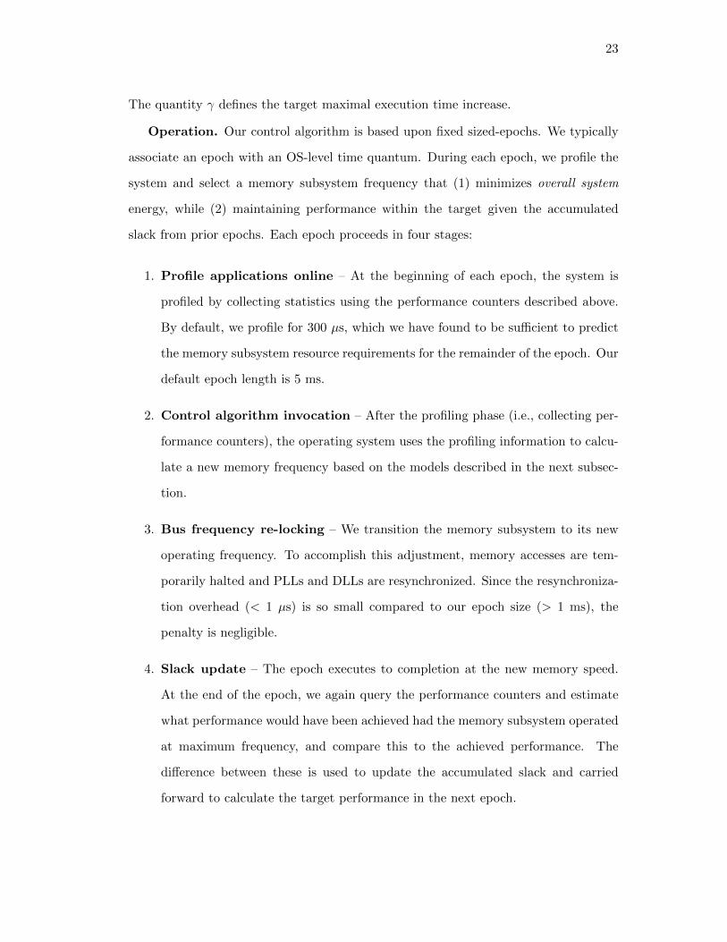
Operation. Our control algorithm is based upon fixed sized-epochs. We typically
associate an epoch with an OS-level time quantum. During each epoch, we profile the
system and select a memory subsystem frequency that (1) minimizes overall system
energy, while (2) maintaining performance within the target given the accumulated
slack from prior epochs. Each epoch proceeds in four stages:
1. Profile applications online – At the beginning of each epoch, the system is
profiled by collecting statistics using the performance counters described above.
By default, we profile for 300 µs, which we have found to be sufficient to predict
the memory subsystem resource requirements for the remainder of the epoch. Our
default epoch length is 5 ms.
2. Control algorithm invocation – After the profiling phase (i.e., collecting per-
formance counters), the operating system uses the profiling information to calcu-
late a new memory frequency based on the models described in the next subsec-
tion.
3. Bus frequency re-locking – We transition the memory subsystem to its new
operating frequency. To accomplish this adjustment, memory accesses are tem-
porarily halted and PLLs and DLLs are resynchronized. Since the resynchroniza-
tion overhead (< 1 µs) is so small compared to our epoch size (> 1 ms), the
penalty is negligible.
4. Slack update – The epoch executes to completion at the new memory speed.
At the end of the epoch, we again query the performance counters and estimate
what performance would have been achieved had the memory subsystem operated
at maximum frequency, and compare this to the achieved performance. The
difference between these is used to update the accumulated slack and carried
forward to calculate the target performance in the next epoch.

24
Note that our policy queries the performance counters both at the end of each
epoch and at the end of each profiling phase. Although we could rely solely on end-of-
epoch accounting, we opt to profile for two main reasons. First, an epoch is relatively
long compared to the length of some applications’ execution phases; a short profiling
phase often provides a more current picture of the applications’ behaviors. Second,
because it may not be possible to monitor all the needed counters at the same time, the
profiling phase can be used to measure just the power-related counters (while only the
performance-related counters would be measured the rest of the time). In this chapter,
we assume that all counters are monitored at the same time.
Frequency selection. We select a memory frequency to achieve two objectives.
First, we wish to select a frequency that maximizes full-system energy savings. The
energy-minimal frequency is not necessarily the lowest frequency—as the system con-
tinues to consume energy when the memory subsystem is slowed, lowering frequency
can result in a net energy loss if the program slowdown is too high. Our models ex-
plicitly account for the system-vs.-memory energy balance. Second, we seek to observe
the bound on allowable CPI degradation for each running program. Because multiple
programs execute within a single system, the selected frequency must satisfy the needs
of the program with the greatest memory performance requirements.
MemScale example. We illustrate the operation of MemScale in Figure 3.1.
Each epoch begins with a profiling phase, shown in gray. Using the profiling output, the
system estimates the performance at the highest memory frequency (“Max Frequency”),
and then sets a target performance (“Target”) via Equation 3.1 above. Based on the
target, a memory speed is selected and the system transitions to the new speed. In
Epoch 1, the example shows that the actual execution (“Actual”) is faster than the
target. Hence, the additional slack is carried forward into Epoch 2, slightly widening
the gap between Max Frequency and Target, allowing the memory speed to be lowered.
However, at the end of Epoch 2, performance falls short of the target, and the negative
slack must be made up in Epoch 3 (or later epochs, if necessary) by raising memory
frequency. By adjusting slack from epoch to epoch, MemScale tries to ensure that the
desired performance target (given by γ) is met over time.

25
Time
Core 1
Core 2
Memory Speed
Epoch 2 Epoch 3 Epoch 4 Epoch 5Epoch 1
Actual
Max FrequencyTarget
Ttr
Ttr TtrTtr
Slack Negative Slack Slack
Slack Negative Slack Slack
Profiling
Figure 3.1: Memscale operation: In this example, we illustrate the operation ofMemScale for two cores. The best-case execution time is calculated at each epoch(“Max Frequency”). The target time is a fixed percent slower than this best case.Slack is the time difference between the target and current execution; it is accumulatedacross epochs. Note that since the frequency transition time, Ttr, is so small comparedto the epoch, the performance penalty is insignificant.
3.2.3 Performance and Energy Models
Now, we describe the performance and energy models that the control algorithm uses
to make smart decisions about frequency.
Performance model. Our control algorithm relies on a performance model to
predict the relationship between CPU cycles per instruction (CPI) of an application
and the memory frequency. The purpose of our model is to determine the runtime
and power/energy implications of changing memory performance. Given this model,
the OS can set the frequency to both maximize energy-efficiency and stay within the
predefined limit for CPI loss.
We model an in-order processor with one outstanding LLC miss per core. We do
so for three reasons: (1) these processors translate any increases in memory access
time due to frequency scaling directly to execution time; (2) we expect server cores to
become simpler as the number of cores per CPU increases; and (3) the modeling of
these processors is simpler than their more sophisticated counterparts, making it easier
to demonstrate our ideas. We approximate the effect of greater memory traffic (e.g.,
resulting from prefetching or out-of-order execution) by varying the number of memory
channels and cores in Section 3.3.2.
26
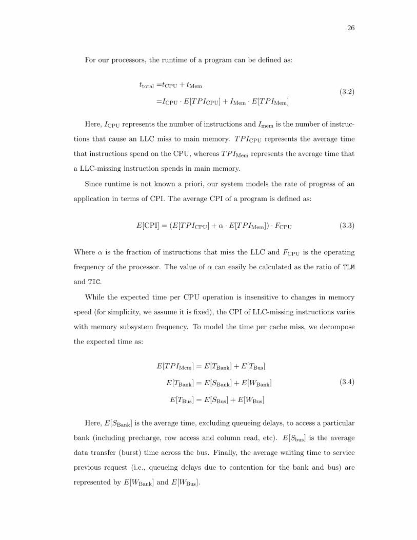
For our processors, the runtime of a program can be defined as:
ttotal =tCPU + tMem
=ICPU · E[TPICPU] + IMem · E[TPIMem]
(3.2)
Here, ICPU represents the number of instructions and Imem is the number of instruc-
tions that cause an LLC miss to main memory. TPICPU represents the average time
that instructions spend on the CPU, whereas TPIMem represents the average time that
a LLC-missing instruction spends in main memory.
Since runtime is not known a priori, our system models the rate of progress of an
application in terms of CPI. The average CPI of a program is defined as:
E[CPI] = (E[TPICPU] + α · E[TPIMem]) · FCPU (3.3)
Where α is the fraction of instructions that miss the LLC and FCPU is the operating
frequency of the processor. The value of α can easily be calculated as the ratio of TLM
and TIC.
While the expected time per CPU operation is insensitive to changes in memory
speed (for simplicity, we assume it is fixed), the CPI of LLC-missing instructions varies
with memory subsystem frequency. To model the time per cache miss, we decompose
the expected time as:
E[TPIMem] = E[TBank] + E[TBus]
E[TBank] = E[SBank] + E[WBank]
E[TBus] = E[SBus] + E[WBus]
(3.4)
Here, E[SBank] is the average time, excluding queueing delays, to access a particular
bank (including precharge, row access and column read, etc). E[Sbus] is the average
data transfer (burst) time across the bus. Finally, the average waiting time to service
previous request (i.e., queueing delays due to contention for the bank and bus) are
represented by E[WBank] and E[WBus].

27
SBank can be further broken down as:
E[SBank] = E[TMC] + E[TDevice] (3.5)
TMC varies as a function of MC frequency. In our MC design, each request requires
five MC clock cycles to process (in the absence of queueing delays). TDevice is a function
of DRAM device parameters and applications’ row buffer hit/miss rates and does not
vary significantly with frequency, as we do not alter the operation or timing of the
DRAM chips’ internal DRAM arrays. During the profiling phase, we estimate E[TDevice]
for the epoch using row buffer performance counters via:
Row hit time = Thit = TCL · RHBC
Closed-bank miss time = Tcb = [TRCD + TCL] · CBMC
Open-bank miss time = Tob = [TRP + TRCD + TCL] · OBMC
Powerdown exit time = Tpd = TXP · EPDC
E[TDevice] =Thit + Tcb + Tob + Tpd
RHBC + CBMC + OBMC
(3.6)
TCL, TRP, TRCD, and TXP are characteristics of a particular memory device and are
obtained from datasheets. To simplify the above equations, we have subsumed some
aspects of DRAM access timing that have smaller impacts.
Whereas modeling SBank and SBus is straight-forward given manufacturer data
sheets, modeling the wait times due to contention E[WBank] and E[WBus] is more chal-
lenging. Ideally, we would like to model the memory system as a queuing network
to determine these quantities. Figure 3.2 shows the queuing model corresponding to
our system. Queueing delays arise due to contention for a bank and the memory bus.
(Delayed requests wait at the MC; there are typically no queues in the DRAM devices
themselves). The in-order CPUs act as users in a closed queuing network (each issuing
a single memory access at a time). Memory requests are serviced by the various banks,
each represented by a queue. The bus is modeled as a server with no queue depth;
when a request completes service at a bank, it must wait at the bank (blocking further

28
Core 1
Core 2
Core N...
Bank 1
Bank 2
Bank 3
Bank 4
Bus -Channel 1
Blocked by Requestat Bus - Channel 1
Figure 3.2: Memory subsystem queuing model: Banks and channels are rep-resented as servers. The cores issue requests to bank servers, which proceed to thechannel server upon completion. Because of DRAM operation, requests are held at thebank server until a request frees from the channel server (the channel server has a queuedepth of 0). In our example, the request that finishes at bank 1 cannot proceed to thebus until the request already there leaves. This example shows only a single channel.
requests) until it is accepted by the bus. This blocking behavior models the activate-
access-precharge command sequence used to access a DRAM bank—the bank remains
blocked until the sequence is complete.
Unfortunately, this queueing network is particularly difficult to analyze. Specifically,
because the system exhibits transfer blocking behavior [4, 7] (disallowing progress at
the bank due to contention at the bus), product form solutions of networks of this size
are infeasible. Most approaches to this problem rely on approximations that have errors
as high as 25% [4, 7]. Instead of using a typical queuing model, we now describe how a
simple counter-based model can yield accurate predictions. We find that the accuracy
afforded by the counters justify their implementation cost.
Our approach is to define counters that track the number of preceding requests
that each arriving request finds waiting ahead of it for a bank/bus. We then take the
expectation of this count over all arrivals to obtain an expression for the expected wait
time for each request. We implement the necessary counters directly in hardware as
described in Section 3.2.1.
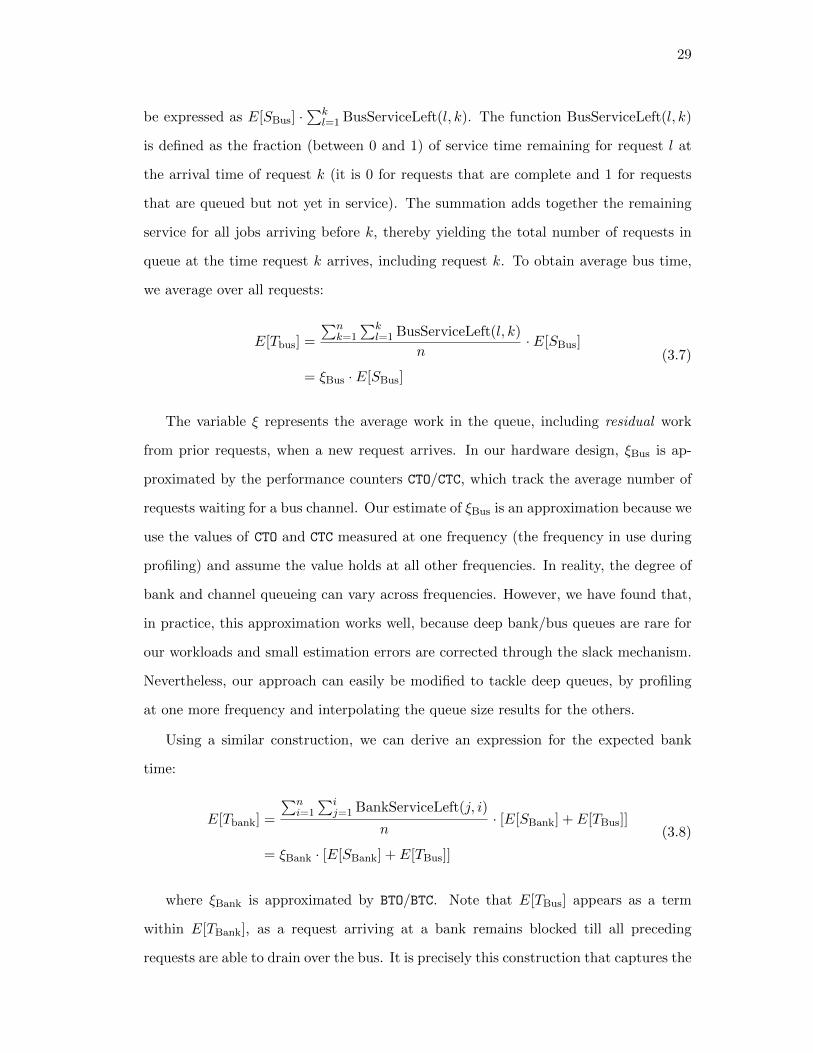
We first illustrate our derivation for bus time. For a single request k, the bus time can
29
be expressed as E[SBus] ·∑k
l=1 BusServiceLeft(l, k). The function BusServiceLeft(l, k)
is defined as the fraction (between 0 and 1) of service time remaining for request l at
the arrival time of request k (it is 0 for requests that are complete and 1 for requests
that are queued but not yet in service). The summation adds together the remaining
service for all jobs arriving before k, thereby yielding the total number of requests in
queue at the time request k arrives, including request k. To obtain average bus time,
we average over all requests:
E[Tbus] =
∑nk=1
∑kl=1 BusServiceLeft(l, k)
n· E[SBus]
= ξBus · E[SBus]
(3.7)
The variable ξ represents the average work in the queue, including residual work
from prior requests, when a new request arrives. In our hardware design, ξBus is ap-
proximated by the performance counters CTO/CTC, which track the average number of
requests waiting for a bus channel. Our estimate of ξBus is an approximation because we
use the values of CTO and CTC measured at one frequency (the frequency in use during
profiling) and assume the value holds at all other frequencies. In reality, the degree of
bank and channel queueing can vary across frequencies. However, we have found that,
in practice, this approximation works well, because deep bank/bus queues are rare for
our workloads and small estimation errors are corrected through the slack mechanism.
Nevertheless, our approach can easily be modified to tackle deep queues, by profiling
at one more frequency and interpolating the queue size results for the others.
Using a similar construction, we can derive an expression for the expected bank
time:
E[Tbank] =
∑ni=1
∑ij=1 BankServiceLeft(j, i)
n· [E[SBank] + E[TBus]]
= ξBank · [E[SBank] + E[TBus]]
(3.8)
where ξBank is approximated by BTO/BTC. Note that E[TBus] appears as a term
within E[TBank], as a request arriving at a bank remains blocked till all preceding
requests are able to drain over the bus. It is precisely this construction that captures the

30
transfer blocking behavior and allows us to sidestep the difficulties of queuing analysis.
Noting that, under this construction, E[TPIMem] = E[Tbank] (bus time has been
folded into the expression for the bank time), we condense our analysis to the equation:
E[TPIMem] = ξbank · (SBank + ξbus · Sbus) (3.9)
Full-system energy model. Simply meeting the CPI loss target for a given work-
load does not necessarily maximize energy-efficiency. In other words, though additional
performance degradation may be allowed, it may save more energy to run faster. To
determine the best operating point, we construct a model to predict full-system energy
usage. For memory frequency fmem, we define the system energy ratio (SER) as:
SER(fmem) =TfMem
· PfMem
TBase · PBase(3.10)
TfMemis the performance estimate for an epoch at frequency fMem. PfMem
=
PMem(fMem) +PNonMem, where PMem(f) is calculated according to the model for mem-
ory power in [65], and PNonMem accounts for all non-memory system components and is
assumed to be fixed. TBase and PBase are corresponding values at a nominal frequency.
At the end of the profiling phase of each epoch, we calculate SER for all memory
frequencies that can meet the performance constraint given by Slack, and select the
frequency that minimizes SER. As we consider only ten frequencies, it is reasonable to
exhaustively search the possibilities and choose the best. In fact, given that this search
is only performed once per epoch (5 ms by default), its overhead is negligible.
3.2.4 Hardware and Software Costs
We now consider the implementation cost of MemScale. The core features in our system
are already available in commodity hardware. Although real servers do not exploit this
capability, existing DIMMs already support multiple frequencies and can switch among
them by transitioning to powerdown or self-refresh states [44]. Moreover, integrated
31
CMOS MCs can leverage existing voltage and frequency scaling technology. One nec-
essary change is for the MC to have separate voltage and frequency control from other
processor components. In recent Intel architectures, this would require separating last-
level cache and MC voltage control [39, 40]. Though processors with multiple frequency
domains are common, there have historically been few voltage domains; however, recent
research has shown this is likely to change soon [32].
Whereas modifying the operating voltage of DIMMs and DRAM circuitry may be
possible, devices with this capability have not yet been marketed commercially. There
are substantial challenges in operating a DRAM array at multiple voltages, as many
circuits in the DRAM access path require precisely tuned timing and transistor sizing
that is specific to the operating voltage. Since we observe significant energy savings
from frequency scaling alone, we restrict our first study to a single voltage level in
DIMMs. Nevertheless, we will consider more aggressive approaches in our future work.
Our design also may require enhancements to hardware performance counters in
some processors. Most processors already expose a set of counters to observe processing,
caching and memory-related performance behaviors (e.g., row buffer hits/misses, row
pre-charges). In fact, Intel’s Nehalem architecture already exposes a number of MC
counters for queues [52]. However, the existing counters may not conform precisely
to the specifications required for our models. As discussed above, the time overhead
of our OS-level policy is negligible, since it is only incurred at the multi-millisecond
granularity.
3.3 Evaluation
3.3.1 Methodology
Simulator and workloads. Since the few hardware mechanisms we propose are not
yet available, our evaluation is based on simulations. To reduce simulation times, our
simulations are done in two steps. In the first step, we use M5 [12] to collect memory
access (LLC misses and writebacks) traces from a variety of workloads running on a
16-core server.
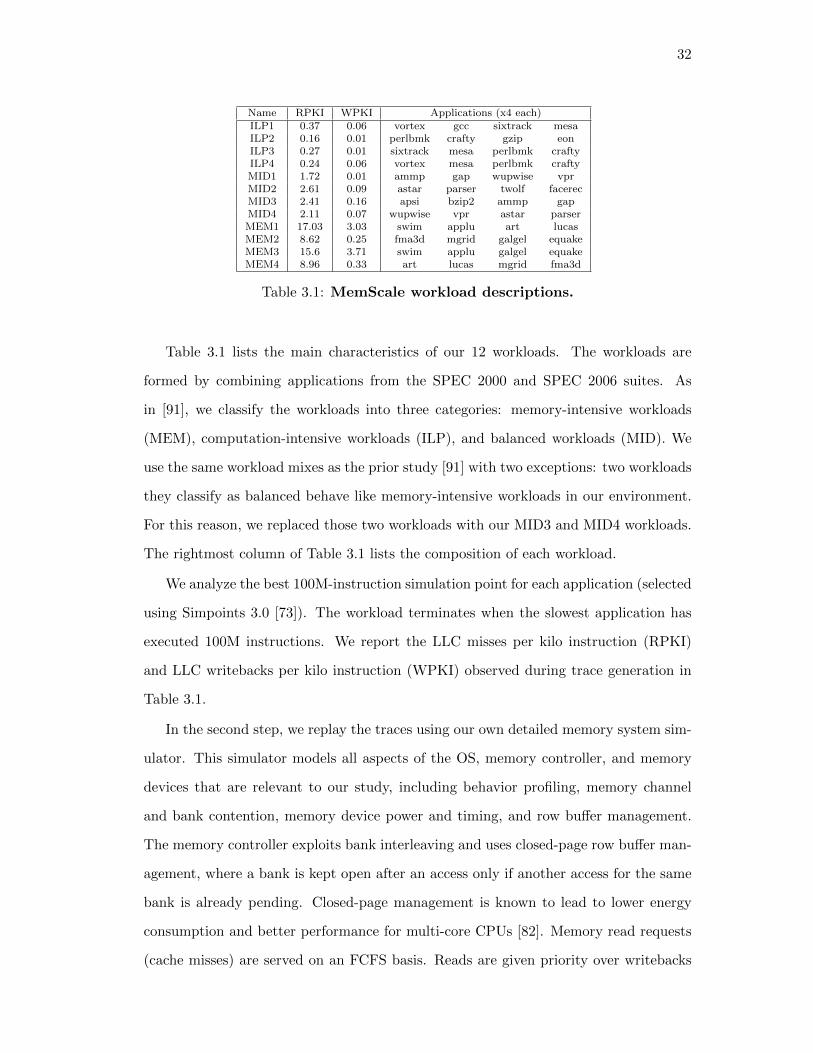
32
Name RPKI WPKI Applications (x4 each)ILP1 0.37 0.06 vortex gcc sixtrack mesaILP2 0.16 0.01 perlbmk crafty gzip eonILP3 0.27 0.01 sixtrack mesa perlbmk craftyILP4 0.24 0.06 vortex mesa perlbmk craftyMID1 1.72 0.01 ammp gap wupwise vprMID2 2.61 0.09 astar parser twolf facerecMID3 2.41 0.16 apsi bzip2 ammp gapMID4 2.11 0.07 wupwise vpr astar parserMEM1 17.03 3.03 swim applu art lucasMEM2 8.62 0.25 fma3d mgrid galgel equakeMEM3 15.6 3.71 swim applu galgel equakeMEM4 8.96 0.33 art lucas mgrid fma3d
Table 3.1: MemScale workload descriptions.
Table 3.1 lists the main characteristics of our 12 workloads. The workloads are
formed by combining applications from the SPEC 2000 and SPEC 2006 suites. As
in [91], we classify the workloads into three categories: memory-intensive workloads
(MEM), computation-intensive workloads (ILP), and balanced workloads (MID). We
use the same workload mixes as the prior study [91] with two exceptions: two workloads
they classify as balanced behave like memory-intensive workloads in our environment.
For this reason, we replaced those two workloads with our MID3 and MID4 workloads.
The rightmost column of Table 3.1 lists the composition of each workload.
We analyze the best 100M-instruction simulation point for each application (selected
using Simpoints 3.0 [73]). The workload terminates when the slowest application has
executed 100M instructions. We report the LLC misses per kilo instruction (RPKI)
and LLC writebacks per kilo instruction (WPKI) observed during trace generation in
Table 3.1.
In the second step, we replay the traces using our own detailed memory system sim-
ulator. This simulator models all aspects of the OS, memory controller, and memory
devices that are relevant to our study, including behavior profiling, memory channel
and bank contention, memory device power and timing, and row buffer management.
The memory controller exploits bank interleaving and uses closed-page row buffer man-
agement, where a bank is kept open after an access only if another access for the same
bank is already pending. Closed-page management is known to lead to lower energy
consumption and better performance for multi-core CPUs [82]. Memory read requests
(cache misses) are served on an FCFS basis. Reads are given priority over writebacks
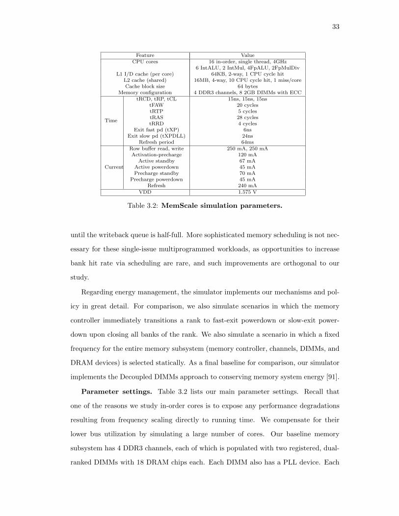
33
Feature ValueCPU cores 16 in-order, single thread, 4GHz
6 IntALU, 2 IntMul, 4FpALU, 2FpMulDivL1 I/D cache (per core) 64KB, 2-way, 1 CPU cycle hit
L2 cache (shared) 16MB, 4-way, 10 CPU cycle hit, 1 miss/coreCache block size 64 bytes
Memory configuration 4 DDR3 channels, 8 2GB DIMMs with ECC
Time
tRCD, tRP, tCL 15ns, 15ns, 15nstFAW 20 cyclestRTP 5 cyclestRAS 28 cyclestRRD 4 cycles
Exit fast pd (tXP) 6nsExit slow pd (tXPDLL) 24ns
Refresh period 64ms
Current
Row buffer read, write 250 mA, 250 mAActivation-precharge 120 mA
Active standby 67 mAActive powerdown 45 mAPrecharge standby 70 mA
Precharge powerdown 45 mARefresh 240 mA
VDD 1.575 V
Table 3.2: MemScale simulation parameters.
until the writeback queue is half-full. More sophisticated memory scheduling is not nec-
essary for these single-issue multiprogrammed workloads, as opportunities to increase
bank hit rate via scheduling are rare, and such improvements are orthogonal to our
study.
Regarding energy management, the simulator implements our mechanisms and pol-
icy in great detail. For comparison, we also simulate scenarios in which the memory
controller immediately transitions a rank to fast-exit powerdown or slow-exit power-
down upon closing all banks of the rank. We also simulate a scenario in which a fixed
frequency for the entire memory subsystem (memory controller, channels, DIMMs, and
DRAM devices) is selected statically. As a final baseline for comparison, our simulator
implements the Decoupled DIMMs approach to conserving memory system energy [91].
Parameter settings. Table 3.2 lists our main parameter settings. Recall that
one of the reasons we study in-order cores is to expose any performance degradations
resulting from frequency scaling directly to running time. We compensate for their
lower bus utilization by simulating a large number of cores. Our baseline memory
subsystem has 4 DDR3 channels, each of which is populated with two registered, dual-
ranked DIMMs with 18 DRAM chips each. Each DIMM also has a PLL device. Each

34
DRAM chip has 8 banks. We study the impact of the most important aspect of the
memory subsystem configuration (the number of memory channels) in Section 3.3.2.
This study also allows us to approximate the effect of the greater memory traffic.
The timing and power parameters of the DRAM chips, register, PLL, and memory
controller are also shown in Table 3.2 [65]. These data are for devices running at 800
MHz. We also consider frequencies of 733, 667, 600, 533, 467, 400, 333, 267, and 200
MHz.
The timing parameters at frequencies other than 800 MHz were computed in the ob-
vious way, according to the aspects of performance that are affected by scaling (Chapter
2). The current parameters at other frequencies were scaled according to Micron’s power
calculator [65]. The transitions between frequencies are assumed to take 512 memory
cycles plus 28 ns. This assumes that frequency can only be changed after going into
fast-exit pre-charge powerdown state and locking the DLLs, as specified in [44]. The
power consumptions of some components also vary with the utilization. Specifically,
the powers of registers and memory controller scale with their respective utilization
linearly from idle to peak power; the PLL power does not scale with utilization. The
register power ranges from 0.25W to 0.5W as a function of utilization, whereas the
memory controller power ranges from 7.5W to 15W [29, 39]. This maximum memory
controller power was taken from [5]. We study the impact of the power proportionality
of the register and the memory controller in Section 3.3.2. We assume that the voltage
of the memory controller varies over the same range as the cores (0.65V-1.2V), as its
frequency changes. Some year-2010 Xeons have an even wider range (e.g., core voltages
in the 7500 series range from 0.675V to 1.35V). In current Xeons, the uncore voltage
range is narrower than that of the cores. However, the uncore domain currently in-
cludes SRAM, which is typically more difficult to voltage-scale than logic. The power
of the memory controller scales with both voltage and frequency. The PLL and register
powers scale linearly with channel frequency.
We do not model power consumption in the non-memory system components in
detail. Rather, we assume that the average power consumption of the DIMMs accounts
for 40% of the total system power, and compute a fixed average power estimate (the
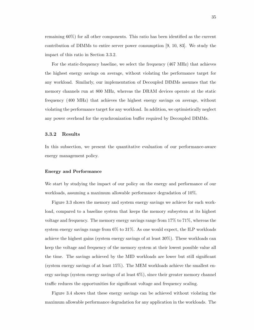
35
remaining 60%) for all other components. This ratio has been identified as the current
contribution of DIMMs to entire server power consumption [9, 10, 83]. We study the
impact of this ratio in Section 3.3.2.
For the static-frequency baseline, we select the frequency (467 MHz) that achieves
the highest energy savings on average, without violating the performance target for
any workload. Similarly, our implementation of Decoupled DIMMs assumes that the
memory channels run at 800 MHz, whereas the DRAM devices operate at the static
frequency (400 MHz) that achieves the highest energy savings on average, without
violating the performance target for any workload. In addition, we optimistically neglect
any power overhead for the synchronization buffer required by Decoupled DIMMs.
3.3.2 Results
In this subsection, we present the quantitative evaluation of our performance-aware
energy management policy.
Energy and Performance
We start by studying the impact of our policy on the energy and performance of our
workloads, assuming a maximum allowable performance degradation of 10%.
Figure 3.3 shows the memory and system energy savings we achieve for each work-
load, compared to a baseline system that keeps the memory subsystem at its highest
voltage and frequency. The memory energy savings range from 17% to 71%, whereas the
system energy savings range from 6% to 31%. As one would expect, the ILP workloads
achieve the highest gains (system energy savings of at least 30%). These workloads can
keep the voltage and frequency of the memory system at their lowest possible value all
the time. The savings achieved by the MID workloads are lower but still significant
(system energy savings of at least 15%). The MEM workloads achieve the smallest en-
ergy savings (system energy savings of at least 6%), since their greater memory channel
traffic reduces the opportunities for significant voltage and frequency scaling.
Figure 3.4 shows that these energy savings can be achieved without violating the
maximum allowable performance degradation for any application in the workloads. The

36
0%
10%
20%
30%
40%
50%
60%
70%
80%
Ene
rgy
Savi
ngs
(%
)
Full System Energy Memory System Energy
Figure 3.3: Energy savings. Memory and full-system energies are significantly re-duced, particularly for the ILP workloads.
figure shows the average and maximum percent CPI losses across the applications in
each of our workloads, again compared to the vanilla baseline. The results demonstrate
that our policy indeed limits the maximum CPI increase to the acceptable range; no
application is ever slowed down more than 9.2%. The results also demonstrate that,
when we average the performance degradations of all the applications in each workload,
this average is never higher than 7.2%. Again, as one would expect, the degradations
are smallest for the ILP workloads, followed by the MID workloads, and then the MEM
workloads.
One might think that the policy could produce even higher energy savings, if it
could keep voltage and frequency low longer and approximate the maximum allowable
degradation more closely. This would increase the memory energy savings. However,
remember that increasing running time also involves consuming more system energy.
Thus, our policy degrades performance only up to the point that this translates into
overall system energy savings.
These energy and performance results are very positive. The ILP workloads can
achieve up to 31% system energy savings for only a maximum performance degradation
of 3.2%. The MID results also exhibit substantial benefits. Even the challenging MEM
workloads achieve up to 9% system energy savings within the allowable performance
degradation. Overall, we observe that MemScale produces average system energy sav-
ings of 18.3% for an average performance degradation of only 4.2%.
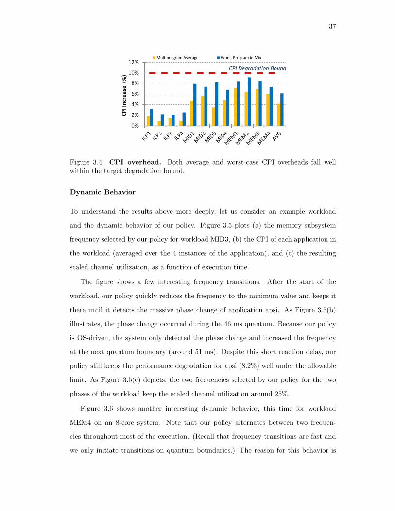
37
0%
2%
4%
6%
8%
10%
12%
CP
I In
cre
ase
(%
)
Multiprogram Average Worst Program in Mix
CPI Degradation Bound
Figure 3.4: CPI overhead. Both average and worst-case CPI overheads fall wellwithin the target degradation bound.
Dynamic Behavior
To understand the results above more deeply, let us consider an example workload
and the dynamic behavior of our policy. Figure 3.5 plots (a) the memory subsystem
frequency selected by our policy for workload MID3, (b) the CPI of each application in
the workload (averaged over the 4 instances of the application), and (c) the resulting
scaled channel utilization, as a function of execution time.
The figure shows a few interesting frequency transitions. After the start of the
workload, our policy quickly reduces the frequency to the minimum value and keeps it
there until it detects the massive phase change of application apsi. As Figure 3.5(b)
illustrates, the phase change occurred during the 46 ms quantum. Because our policy
is OS-driven, the system only detected the phase change and increased the frequency
at the next quantum boundary (around 51 ms). Despite this short reaction delay, our
policy still keeps the performance degradation for apsi (8.2%) well under the allowable
limit. As Figure 3.5(c) depicts, the two frequencies selected by our policy for the two
phases of the workload keep the scaled channel utilization around 25%.
Figure 3.6 shows another interesting dynamic behavior, this time for workload
MEM4 on an 8-core system. Note that our policy alternates between two frequen-
cies throughout most of the execution. (Recall that frequency transitions are fast and
we only initiate transitions on quantum boundaries.) The reason for this behavior is

38
mel i ne
0
5
10
15C
PI
apsi
bzip2
ammp
gap
(b)
0
200
400
600
800
Bu
s Fr
eq
(M
Hz) (a)
0%
20%
40%
60%
80%
100%
0 50 100
Ch
ann
el U
tiliz
atio
n
Time (ms)
ch0
ch1
ch2
ch3
(c)
Figure 3.5: Timeline of MID3 workload in MemScale MemScale adjusts memorysystem frequency rapidly in response to the phase change in apsi.
0
200
400
600
800
Bu
s Fr
eq
(M
Hz)
(a)
02468101214
0 50 100
CP
I
Time (ms)
art
lucas
mgrad
fma3d
(b)
Figure 3.6: Timeline of MEM4 workload in MemScale. MemScale approximatesa “virtual frequency” by oscillating between two neighboring frequencies.
39
that the space of usable frequencies is not continuous; the ideal frequency is really be-
tween the two usable frequencies. In essence, our policy defines a “virtual frequency”
by alternating between the two frequencies.
Comparison with Other Policies
In this subsection, we compare our MemScale policy (“MemScale”) to six alterna-
tives. The first alternative (“Fast-PD”) represents today’s aggressive memory con-
trollers, which immediately transition a rank to fast-exit precharge powerdown state
whenever the last open bank of the rank is closed. The second alternative (“Slow-PD”)
is even more aggressive in that it transitions the rank to slow-exit precharge powerdown
state. The third alternative (“Decoupled”) is the decoupled DIMM approach to energy
conservation, which combines low-frequency memory devices with high-frequency chan-
nels. The fourth alternative (“Static”) represents the scenario in which the frequency
for the memory controller, channels, DIMMs, and DRAM devices is selected statically
before the workloads are started. The fifth and sixth alternatives are actually variations
of our policy. The fifth (“MemScale (MemEnergy)”) considers only the memory energy
(rather than the overall system energy) in making decisions. The sixth (“MemScale +
Fast-PD”) is our full policy combined with fast-exit powerdown.
Figure 3.7 shows the average energy savings achieved by all alternatives, across the
MID workloads. For these same workloads, Figure 3.8 breaks down the average system
power of each alternative between its DRAM, PLL/register, memory controller, and
rest-of-the-system (everything but the memory subsystem) components. Figure 3.9
shows the average and maximum performance degradations for all the alternatives,
again across the same workloads. All results are computed with respect to the baseline,
which keeps the memory subsystem at its highest frequency at all times.
These results demonstrate that Fast-PD achieves small energy savings at small per-
formance degradations. The energy savings come from reductions in the power con-
sumption of the DRAM chips. For the MEM and ILP workloads, Fast-PD achieved
system energy savings between 0.3% (MEM2) and 7.4% (ILP3). Being more aggres-
sive with Slow-PD actually hurts performance so much that the workloads consume

40
0%5%
10%15%20%25%30%35%40%45%50%
Ene
rgy
Savi
ngs
(%
)
Full System Energy Memory System Energy
Figure 3.7: Energy savings. MemScale provides greater full-system and memorysystem energy savings than alternatives.
0
0.2
0.4
0.6
0.8
1
Energy
(No
rmal
ized
Cto
CBas
e)
DRAM PLL/Reg. MC RestCofCsystem
Figure 3.8: System energy breakdown. MemScale reduces DRAM, PLL/Reg, andMC energy more than alternatives.
0%
2%
4%
6%
8%
10%
12%
14%
CP
I In
cre
ase
(%
)
Multiprogram Average Worst Program in Mix
Figure 3.9: CPI overhead. MemScale’s CPI increases are under 10%. MemScale(MemEnergy) slightly exceeds the bound.

41
more system energy than the baseline system. In fact, the performance of one of the
applications actually degrades by 15%. Both of these results match expectations.
In contrast, Decoupled does better than Fast-PD or Slow-PD. It achieves higher
energy savings at moderate performance degradations for the MID workloads. The
energy savings come from reductions in the power consumed by the DRAM devices.
Decoupled also does well for the ILP workloads, achieving a maximum energy savings
of 11%. However, it actually increases the energy consumption for one of the MEM
workloads (MEM3) by 0.8%. This result is due to a significant performance degradation
for this workload.
Static conserves more memory and system energy than Decoupled (for roughly the
same performance degradations), despite the fact that the frequency of the DRAM
devices is lower under Decoupled than Static (400 vs 467 MHz). This arises because
Static decreases the energy consumption of the memory controller and the PLL/register
devices. Decoupled does not address these sources of energy consumption. DRAM
device energy is indeed lower under Decoupled, as one would expect. Static also does
well for the ILP and MEM workloads, achieving average system energy savings of 19.1%
and 7.8%, respectively, always within the allowed performance degradation.
MemScale easily outperforms Decoupled. We achieve almost 3x higher energy sav-
ings, while keeping degradation within the allowed range. The reason for this result
is that MemScale can dynamically adjust frequencies and achieve energy gains in the
memory controller and PLL/register as well.
MemScale is also superior to Static in both memory and system energy savings,
but leads to slightly (2%) higher performance degradations. Specifically, MemScale’s
average system energy savings is 30.2% for the ILP workloads and 16.9% for the MID
workloads, whereas Static achieves only 19.1% and 14.5% savings, respectively. (Their
savings for the MEM workloads are comparable.) Our greater energy savings come
from MemScale’s ability to dynamically adjust frequency to the exact conditions of
each workload. Under the unrealistic assumption that the user would (1) manually
select the best frequency for each workload, and (2) somehow instruct the server to
reboot to the new frequency before running the workload, Static and MemScale would

42
differ little for the workloads that do not exhibit dynamic phase changes. For those that
do, MemScale would still surpass Static through dynamically adjusting the frequency,
as seen in the MID3 workload, for example.
As we suggested before, when our policy is set to consider memory energy and not
system energy (MemScale (MemEnergy)), the system conserves more memory energy
but at the cost of system energy and performance. Moreover, note that MemScale
(MemEnergy) exceeds the performance target by just 0.8% for two applications, each
in a different workload. The reason is that MemScale sometimes mispredicts the queue
lengths of the highest memory frequency. These mispredictions affect MemScale’s com-
putation of the performance slack.
Interestingly, note that adding Fast-PD to MemScale does not meaningfully improve
its results; the average system energy savings stay roughly the same (lower DRAM
chip power but higher rest-of-the-system power), whereas the performance degradations
worsen slightly.
Sensitivity Analysis
In this subsection, we investigate the effect of our main simulation and policy para-
meters: the maximum allowable performance degradation, the configuration of the
channels and DIMMs, the fraction of the memory power with respect to the whole
server power, the power proportionality of the memory controller and DIMMs’ regis-
ters, the length of the OS quantum, and the length of the profiling period. We again
perform these studies using the MID workloads.
Maximum performance degradation. This parameter is important in that
higher allowable degradations could enable greater energy savings. To understand the
impact of this parameter, Figure 3.10 illustrates the energy savings (bars on the left)
and maximum achieved degradations (bars on the right), for maximum allowable degra-
dations of 1%, 5%, 10%, and 15%. Recall that our default maximum allowable degrada-
tion is 10%. All other parameters remain at their defaults. It is interesting to observe
that 1% and 5% degradations indeed produce lower energy savings. However, allowing
15% degradation does not improve our savings: beyond a certain point, lengthening the

43
0%
5%
10%
15%
20%
System Energy Reduction Worst-case CPI Increase
1% bound
5% bound
10% bound
15% bound
Figure 3.10: Impact of CPI bound. Increasing the bound beyond 10% does not yieldfurther energy savings.
execution to conserve more memory energy actually increases overall energy. At that
point, our policy stops lowering frequency.
Amount of memory traffic. As far as MemScale is concerned, the number of
channels is the most important aspect of the memory subsystem configuration. The
number of channels directly affects how heavily utilized each channel is and, thus, our
opportunities to lower frequency without excessively degrading performance. In fact,
decreasing the number of channels approximates the effect of greater memory traffic that
could result from prefetching or out-of-order execution. Figure 3.11 depicts the energy
savings (left) and maximum achieved performance degradation (right) for 2, 3, and 4
channels. Recall that our default results assumed 4 channels. The figure shows that
increases in the number of channels indeed increase the benefits of MemScale by non-
trivial amounts, without affecting our ability to limit performance losses. Interestingly,
the figure also shows that doubling the channel traffic (from 4 to 2 channels) still leads
to system energy savings of roughly 14%.
Another approach for studying the effect of greater memory traffic is to increase the
number of cores, while keeping the LLC size the same. Thus, we performed experiments
with 32 cores and 4 memory channels. For the MID workloads, the larger number of
cores causes 2x-4x increases in traffic. These increases translate into system energy
savings ranging from 7.6% to 10.4%, without any violations of the performance bound.
Fraction of memory system power with respect to server power. Because
44
0%
5%
10%
15%
20%
System3Energy3Reduction Worst-case3CPI3Increase
43channels
33channels
23channels
Figure 3.11: Impact of number of channels. MemScale provides greater savingswhen there are more, less-utilized channels.
0%
5%
10%
15%
20%
25%
System Energy Reduction Worst-case CPI Increase
30% Mem
40% Mem
50% Mem
Figure 3.12: Impact of fraction of memory power. Increasing the fraction increasesenergy savings.
MemScale seeks to reduce whole-system energy consumption by reducing the memory
subsystem energy, the contribution of the memory subsystem to the overall power con-
sumption of the server becomes a crucial parameter. Intuitively, the larger this fraction,
the larger our percentage energy savings. Furthermore, recall that the non-memory-
subsystem power consumption affects our energy management policy. Intuitively, the
lower the non-memory-subsystem contribution, the lower the frequencies that our policy
can select. Figure 3.12 quantifies the impact of 30%, 40%, and 50% fractions of mem-
ory power on the system energy savings. Recall that our baseline assumes a fraction of
40%.
The figure shows that the fraction of memory power has a significant effect on the
system energy savings. Increasing the fraction from 30% to 50% (or, equivalently,
reducing the rest-of-the-system contribution from 70% to 50%) more than doubles the
savings (11% vs 24%). The maximum CPI degradation increases by a few percent as
well, but stays within the allowed range.
Power proportionality of the memory controller and DIMMs’ registers.

45
0%
5%
10%
15%
20%
25%
System Energy Reduction Worst-case CPI Increase
0% Idle Power
50% Idle Power
100% Idle Power
Figure 3.13: Impact of power proportionality of MC and registers. Decreasingproportionality increases energy savings.
Since the memory controller and DIMM register designs are vendor- and model-dependent,
we studied a wide range of power proportionality possibilities for these components.
Specifically, we varied their idle power consumption from 0% (perfect proportionality)
to 100% (no proportionality) of their peak power consumption. Recall that our default
assumption is 50% idle power for these components. For this analysis (and our other
results), we assume that their power consumption changes linearly with utilization be-
tween idle and peak loads. Figure 3.13 depicts the results.
The figure shows that the power proportionality of these components has a signif-
icant impact on the system energy savings. Interestingly, decreasing proportionality
actually increases our savings significantly to 23%. As the memory subsystem’s idle
power increases (decreasing proportionality), the scope of MemScale to reduce register
and memory controller power grows. Importantly, MemScale achieves these benefits
without violating the allowed performance degradation.
Length of the OS quantum (epoch) and profiling period. We studied the
effect of (1) the epoch length by considering quanta of 1, 5, and 10ms; and (2) the
length of the profiling period by considering periods of 0.1, 0.3, and 0.5ms. The first
study sought to assess our ability to stay within the performance requirement, even
when our decisions could not be changed for long periods of time. Similarly, the goal
of the second study was to assess the need for long profiling periods before making
decisions. Overall, these studies revealed that MemScale is essentially insensitive to
reasonable values of these parameters.

46
3.4 Conclusion
In this chapter, we proposed the MemScale approach to managing memory energy under
performance constraints. MemScale creates and leverages active low-power modes that
result from dynamically scaling the frequency of memory channels and DRAM devices,
and dynamically scaling the voltage and frequency of the memory controller. We also
proposed a small set of mechanisms and an operating system policy to determine the
best power mode at each point in time. Our evaluation demonstrated that MemScale
conserves significant memory and system energy, while staying within pre-set perfor-
mance limits. Our results also showed that MemScale is superior to four competing
energy management techniques. We conclude that MemScale’s potential benefits far
outweigh its small hardware costs.

47
Chapter 4
CoScale
4.1 Introduction
In Chapter 3, we proposed MemScale, a set of active low-power modes, hardware mech-
anisms, and software policies to conserve system energy. MemScale achieves this by
targeting at the power consumption of the main memory subsystem including the MC.
Obviously, one can potentially accrue even greater energy savings by targeting the pro-
cessors as well. There is a rich array of processor power management techniques already,
e.g. [36, 45, 80]. Moreover, future servers are likely to provide separate power man-
agement capabilities for individual system components, with distinct control policies
and actuation mechanisms. Our ability to maximize energy efficiency will hinge on the
coordinated use of these various capabilities [62].
Prior work on the coordination of CPU power and thermal management across
servers, blades, and racks has demonstrated the difficulty of coordinated management
and the potential pitfalls of independent control [76]. Existing studies seeking to co-
ordinate CPU DVFS and memory low-power modes have focused on idle low-power
memory states [15, 25, 55]. While effective, these works ignore the possibility of using
DVFS for the memory subsystem, which has been shown to provide greater energy sav-
ings in MemScale. As such, the coordination of active low-power modes for processors
and memory in tandem remains an open problem.
In this chapter, we propose CoScale, the first method for effectively coordinating
CPU and memory subsystem DVFS under performance constraints. As we show, simply
supporting separate processor and memory energy management techniques is insuffi-
cient, as independent control policies often conflict, leading to oscillations, unstable
behavior, or sub-optimal power/performance trade-offs.

48
To see an example of such behavior, consider a scenario in which a chip multi-
processor’s cores are stalled waiting for memory a significant fraction of the time. In
this situation, the CPU power manager might predict that lowering voltage/frequency
will improve energy efficiency while still keeping performance within a pre-selected per-
formance degradation bound and effect the change. The lower core frequency would
reduce traffic to the memory subsystem, which in turn could cause its (independent)
power manager to lower the memory frequency. After this latter frequency change,
the performance of the server as a whole may dip below the CPU power manager’s
projections, potentially violating the target performance bound. So, at its next oppor-
tunity, the CPU manager might start increasing the core frequency, inducing a similar
response from the memory subsystem manager. Such oscillations waste energy. These
unintended behaviors suggest that it is essential to coordinate power-performance man-
agement techniques across system components to ensure that the system is balanced to
yield maximal energy savings.
To accomplish this coordinated control, we rely on execution profiling of core and
memory access performance, using existing and new performance counters. Through
counter readings and analytic models of core and memory performance and power
consumption, we assess opportunities for per-core voltage and frequency scaling in a
chip multiprocessor, voltage and frequency scaling of the on-chip memory controller,
and frequency scaling of memory channels and DRAM devices.
The fundamental innovation of CoScale is the way it efficiently searches the space
of per-core and memory frequency settings (we set voltages according to the selected
frequencies) in software. Essentially, our epoch-based policy estimates, via our perfor-
mance counters and online models, the energy and performance cost/benefit of altering
each component’s (or set of components’) DVFS state by one step, and iterates to greed-
ily select a new frequency combination for cores and memory. The selected combination
trades off core and memory scaling to minimize full-system energy while respecting a
user-defined performance degradation bound. CoScale is implemented in the operating
system (OS), so an epoch typically corresponds to an OS time quantum.

49
For comparison, we demonstrate the limitations of fully uncoordinated and semi-
coordinated control (i.e., independent controllers that share a common estimate of
target and achieved performance) of processor and memory DVFS. These strategies
either violate the performance bound or oscillate wildly before settling into local min-
ima. Uncoordinated policy can not bound the performance well since independent
DVFS controllers both try to consume the same performance slack without knowing
the existence of each other; Semicoordinated policy causes interference between two
DVFS controllers and leads to wild oscillation, and at the end frequencies configuration
usually converges onto some local minimals causing poor energy efficiency.
CoScale circumvents these problems by assessing processor and memory perfor-
mance in tandem. In fact, CoScale provides energy savings close to an offline scheme
that considers an exponential space of possible frequency combinations. We also quan-
tify the benefits of CoScale versus CPU-only and memory-only DVFS policies.
Our results show that CoScale provides up to 24% full-system energy savings (16%
on average) over a baseline scheme without DVFS, while staying within a 10% allow-
able performance degradation. Furthermore, we study CoScale’s sensitivity to several
parameters, including its effectiveness across performance bounds of 1%, 5%, 15%, and
20%. Our results demonstrate that CoScale meets the performance constraint while
still saving energy in all cases.
The remainder of the chapter is structured as follows. Section 4.2 describes CoScale
in detail. Section 4.3 describes our evaluation methodology and results. Finally, Section
4.4 concludes the chapter.
4.2 CoScale Design
In this section, we describe CoScale’s approach for maximizing full-system energy sav-
ings under a performance loss bound. First, we describe our policy at a high level.
Next, we describe its algorithm for selecting frequencies and compare it with simpler
algorithms. We then present the details behind CoScale, including the performance

50
counters and performance/power models that it requires. Finally, we address imple-
mentation costs.
CoScale leverages three key mechanisms: core and memory subsystem DVFS, and
a performance management scheme that keeps track of how much energy conservation
has slowed down applications.
Core DVFS. We assume that each core can be voltage and frequency scaled inde-
pendently of the other cores, as in [46, 89]. We also assume the shared L2 cache sits
in a separate voltage domain that does not scale. A core DVFS transition takes a few
10’s of microseconds.
Memory DVFS. Our memory DVFS method is based on MemScale, which dynam-
ically adjusts MC, bus, and DIMM frequencies. Although it adjusts these frequencies
together, we shall simply refer to adjusting the bus frequency. The DIMM clocks lock
to the bus frequency (or a multiple thereof), while the MC frequency is fixed at double
the bus frequency. Furthermore, MemScale adjusts the voltage of the MC (indepen-
dently of core/cache voltage) and PLL/register in the DIMMs, based on the memory
subsystem frequency.
Memory mode transition time is dominated by frequency re-calibration of the mem-
ory channels and DIMMs. The DIMM operating frequency may be reset while in the
precharge powerdown or self-refresh state. We use precharge powerdown because its
overhead is significantly lower than that of self-refresh. Most of the re-calibration la-
tency is due to the DLL synchronization time, tDLLK [64]—approximately 500 memory
cycles.
Performance management. Similar to the approach initially proposed in [56]
and later explored in [22, 70], our policy is based on the notion of program slack : the
difference between a baseline execution and a target latency penalty that a system op-
erator is willing to incur on a program to save energy. The basic idea is that energy
management often necessitates running the target program with reduced core or mem-
ory subsystem performance. To constrain the impact of this performance loss, CoScale
dictates that each executing program incurs no more than a pre-selected maximum
slowdown γ, relative to its execution without energy management (TMaxFreq). Thus,

51
Slack = TMaxFreq(1 + γ)− TActual.
Overall operation. CoScale uses fixed-size epochs, typically matching an OS time
quantum. Each epoch consists of a system profiling phase followed by the selection of
core and memory subsystem frequencies that (1) minimize full system energy, while (2)
maintaining performance within the target given by the accumulated slack from prior
epochs.
In the system profiling phase, performance counters are read to construct application
performance and energy estimates. By default, we profile for 300 µs, which we find to
be sufficient to predict the resource requirements for the remainder of the epoch. Our
default epoch length is 5 ms.
Based on the profiling phase, the OS selects and transitions to new core and/or
memory bus frequencies using the algorithm described below. During a core transition,
that core does not execute instructions; other cores can operate normally. To adjust
the memory bus frequency, all memory accesses are temporarily halted, and PLLs and
DLLs are resynchronized. Since the core and memory subsystem transition overheads
are small (tens of microseconds) compared to our epoch size (milliseconds), the penalty
is negligible.
The epoch executes to completion with the new voltages and frequencies. At the
end of the epoch, CoScale again estimates the accumulated slack, by querying the
performance counters and estimating what performance would have been achieved had
the cores and the memory subsystem operated at maximum frequency. These estimates
are then compared to achieved performance, with the difference used to update the
accumulated slack and carried forward to calculate the target performance in the next
epoch.
CoScale example. Figure 4.1 depicts an example of CoScale’s behavior (bottom),
compared to a policy that does not fully coordinate the processor and memory frequency
selections (top). We refer to the latter policy as semi-coordinated, as it maintains a sin-
gle performance slack (a mild form of coordination) that is shared by separate CPU and
memory power state managers. As the figure illustrates, under semi-coordinated con-
trol, the CPU manager and the memory manager independently decide to scale down

52
Actual performance
CPU frequency
Memory frequency
Actual performance
Perf. Target
Perf. Target
Profiling
Sem
i-co
ord
inat
edC
oSc
ale
Time
Profiling
CPU frequency
Memory frequency
Figure 4.1: CoScale operation: Semi-coordinated oscillates, whereas CoScale scalesfrequencies more accurately.
when they observe performance slack (performance above target). Unfortunately, be-
cause they are unaware of the cumulative effect of their decisions, they over-correct
by scaling frequency too far down. For the same reason, in the following epoch, they
over-react again by scaling frequency too far up. Such over-reactions continue in an
oscillating manner. With CoScale, by modeling the joint effect of CPU and mem-
ory scaling, the appropriate frequency combination can be chosen to meet the precise
performance target. Our control policy avoids both over-correction and oscillation.
4.2.1 CoScale’s Frequency Selection Algorithm
When choosing a frequency for each core and a frequency for the memory bus, we have
two goals. First, we wish to select a frequency combination that maximizes full-system
energy savings. The energy-minimal combination is not necessarily that with the lowest
frequencies; lowering frequency can increase energy consumption if the slowdown is too
high. Our models explicitly account for the system-vs.-component energy balance.
Fortunately, the cores and memory subsystem consume a large fraction of total system
power, allowing CoScale to aggressively consume the performance slack. Second, we
seek to observe the bound on allowable cycles per instruction (CPI) degradation for

53
each running program.
Dynamically selecting the optimal frequency settings is challenging, since there are
M ×CN possibilities, where M is the number of memory frequencies, C is the number
of possible core frequencies, and N is the number of cores. M and C are typically
on the order of 10, whereas N is in the range of 8-16 now but is growing fast. Thus,
CoScale uses the greedy heuristic policy described in Figure 4.2.
Our gradient-descent heuristic iteratively estimates, via our online models, the
marginal benefit (measured as ∆power/∆performance) of altering either the frequency
of the memory subsystem or that of various groups of cores by one step (we discuss
core grouping in detail below). Initially, the algorithm estimates performance assuming
all cores and memory are set to their highest possible frequencies (line 1 in the figure).
It then iteratively considers frequency reductions, as long as some frequency can still
be lowered without violating the performance slack (loop starting in line 2). When
presented with a choice between next scaling down memory or a group of cores, the
heuristic greedily selects the choice that will produce the highest marginal benefit (lines
3-12). If only memory or only cores can be scaled down, the available option is taken
(line 13-19). Still in the main loop, the algorithm computes and records the full-system
energy ratio (SER, Section 4.2.3) for the considered frequency configuration. When
no more frequency reductions can be tried without violating the slack, the algorithm
selects the configuration yielding the smallest SER (i.e., the best full-system energy
savings) (line 21) and directs the hardware to transition frequencies (line 22).
Changing the frequency of the memory subsystem impacts the performance of all
cores. Thus, when we compute the ∆performance of lowering memory frequency,
we choose the highest performance loss of any core. Similarly, when computing the
∆performance of lowering the frequencies of a group of cores, we consider the worst
performance loss in the group. The ∆power in these cases is the power reduction that
can be achieved by lowering the frequency of each core in the group.
An important aspect of the CoScale heuristic is that it considers lowering the fre-
quency of cores in groups of 1, 2, 3, ..., N cores (lines 1-6 in Figure 4.3). The group

54
1. Estimate performance with each core and the memory subsystem at their highest frequencies
2. While any component can be scaled down further without slack violation
3. If both memory and at least one core can still scale down by 1 step
4. If the memory frequency has changed since we last computed marginal_memory
5. Compute marginal utility of lowering memory frequency as marginal_memory
6. If any core frequency has changed since we last computed marginal_cores
7. Compute marginal utility of lowering the frequency of core groups (per algorithm in Figure 4.3)
8. Select the core group (group_best) with the largest utility (marginal_cores)
9. If marginal_memory is greater than marginal_cores
10. Scale down memory by 1 step
11. Else
12. Scale down cores in group_best by 1 step each
13. Else if only memory can scale down
14. Scale down memory by 1 step
15. Else if only core groups can scale down
16. If any core frequency has changed since we last computed marginal_cores
17. Compute marginal utility of lowering the frequency of core groups (per algorithm in Figure 4.3)
18. Select the core group (group_best) with largest marginal utility (marginal_cores)
19. Scale down cores in group_best by 1 step each
20. Compute and record the SER for the current combination of core and memory frequencies
21. Select the core and memory frequency combination with the smallest SER
22. Transition hardware to the new frequency combination
Figure 4.2: CoScale’s greedy gradient-descent frequency selection algorithm.
1. Scan the previous list of cores, removing any that may not scale down further or whose frequency
has changed
2. Re-insert cores with changed frequency, maintaining an ascending sort order by delta performance
3. For group i from 1 to number of cores on the list
4. Let delta power of the i-th group be equal to the sum of delta power from first to the i-th core
5. Let delta performance be equal to delta performance of the i-th core
6. Let marginal utility of i-th group be equal to delta power over delta performance just calculated
7. Set the group with the largest marginal utility as the best group (group_best) and its utility as
marginal_cores
Figure 4.3: Sub-algorithm to consider core frequency changes by group.
formation algorithm maintains a list of cores that are eligible to scale down in fre-
quency (i.e., they can be scaled down without slack violation), sorted in ascending
order of ∆performance. To avoid a potentially expensive sort operation on each invo-
cation, the algorithm updates the existing sorted list by removing and then re-inserting
only those cores whose frequency has changed (lines 1-2). N possible core groups are
considered, forming groups greedily by first selecting the core that incurs the smallest
delta performance from scaling (i.e., just the head of the list), then considering this
core and the second core, then the third, and so on. This greedy group formation
avoids combinatorial state space explosion, but, as we will show, it performs similarly
to an offline method that considers all combinations. Considering transitions by group
is needed to prevent CoScale from always lowering memory frequency first, because the

55
memory subsystem at first tends to provide greater benefit than scaling any one core
in isolation. Failing to consider group transitions may cause the heuristic to get stuck
in local minima.
Our algorithm is run at the end of the profiling phase of each epoch (5ms by default).
Because of core grouping, the complexity of our heuristic is O(M + C ×N2), which is
exponentially better than that of the brute-force approach. Given our default simula-
tion settings for M (10), C (10), and N (16), searching once per epoch has negligible
overhead. Specifically, in all our experiments, searching takes less than 5 microseconds
on a 2.4GHz Xeon machine. Our projections for larger core counts suggest that the
algorithm could take 83 and 360 microseconds for 64 and 128 cores, respectively, in the
worst case (4 microseconds in the best case). If one finds it necessary to hide these
higher overheads, one can either increase the epoch length or dedicate a spare core to
the algorithm.
4.2.2 Comparison with Other Policies
The key aspect of CoScale is the efficient way in which it searches the space of possible
CPU and memory frequency settings. For comparison, we study five alternatives. The
first is “MemScale”, represents the scenario in which the system uses only memory
subsystem DVFS. The second alternative, called “CPUOnly”, represents the scenario
with CPU DVFS only. To be optimistic about this alternative, we assume that it
considers all possible combinations of core frequencies and selects the best. In both
MemScale and CPUOnly, the performance-aware energy management policy assumes
that the behavior of the components that are not being managed will stay the same in
the next epoch as in the profiling phase.
The third alternative, called “Uncoordinated”, applies both MemScale and CPU
DVFS, but in a completely independent fashion. In determining the performance slack
available to it, the CPU power manager assumes that the memory subsystem will remain
at the same frequency as in the previous epoch, and that it has accumulated no CPI
degradation; the memory power manager makes the same assumptions about the cores.
Hence, each manager believes that it alone influences the slack in each epoch, which is

56
not the case. The fourth alternative, called “Semi-coordinated”, increases the level of
coordination slightly by allowing the CPU and memory power managers to share the
same overall slack, i.e. each manager is aware of the past CPI degradation produced by
the other. However, each manager still tries to consume the entire slack independently
in each epoch (i.e., the two managers account for one another’s past actions, but do
not coordinate their estimate of future performance).
Finally, the fifth alternative, called “Offline”, relies on a perfect offline performance
trace for every epoch, and then selects the best frequency for each epoch by considering
all possible core and memory frequency settings. As the number of possible settings
is exponential, Offline is impractical and is studied simply as an upper bound on how
well CoScale can do. However, Offline is not necessarily optimal, since it uses the same
epoch-by-epoch greedy decision-making as CoScale (i.e., a hypothetical oracle might
choose to accumulate slack in order to spend it in later epochs).
Figure 4.4 visualizes the difference between CoScale and other policies in terms
of their search behaviors. For clarity, the figure considers only two cores (X and Y
axes) and the memory (Z axis), forming a 3-D frequency space. The origin point is the
highest frequency of each dimension; more distant points represent lower per-component
frequencies. CPUOnly and MemScale search subsets of these three dimensions, so we
do not illustrate them.
We can see from the figure that the Offline policy (top illustration) examines the
entire space, thus always finding the best configuration. Under the Uncoordinated
policy (second row), the CPU power manager tries to consume as much of the slack
as possible with cores 0 and 1, while the memory power manager gets to consume the
same slack. This repeats every epoch. Semi-coordinated (third row) behaves similarly
in the first epoch. However, in the second epoch, to correct for the overshoot in the
first epoch, each manager is restricted to a smaller search space. This restriction leads
to over-correction in the third epoch, resulting in a much larger search space. The
resulting oscillation may continue across many epochs. Finally, CoScale (bottom row)
starts from the origin and greedily considers steps of memory frequency or (groups
of) core frequency, selecting the move with the maximal marginal energy/performance

57
Core 0Frequency
Mem
ory
Fre
quen
cy
Core
1
Frequ
encyUn
coo
rdin
ated
Core 0Frequency
Mem
ory
Fre
quen
cy
Core
1
Frequ
ency
Of
ine
Core 0Frequency
Mem
ory
Fre
quen
cy
Core
1
Frequ
ency
Co
Sca
le
Core 0Frequency
Mem
ory
Fre
quen
cy
Core
1
Frequ
ency
Core 0Frequency
Mem
ory
Fre
quen
cy
Core
1
Frequ
ency
Core 0Frequency
Mem
ory
Fre
quen
cy
Core
1
Frequ
ency
Core 0Frequency
Mem
ory
Fre
quen
cy
Core
1
Frequ
ency
Sem
i-co
ord
inat
ed
Core 0Frequency
Mem
ory
Fre
quen
cy
Core
1
Frequ
ency
Core 0Frequency
Mem
ory
Fre
quen
cy
Core
1
Frequ
ency
Core 0Frequency
Mem
ory
Fre
quen
cy
Core
1
Frequ
ency
One epochOne epochEpoch 1
Epoch 1 Epoch 2 Epoch 3
Epoch 1 Epoch 2 Epoch 3
Epoch 1: step 1 Epoch 1: step 2 Epoch 1: step 3
Figure 4.4: Search differences: CoScale searches the parameter space efficiently. Uncoordi-nated violates the performance bound and Semi-coordinated gets stuck in local minima.

58
benefit. From the figure, we can see that in step 1, CoScale scaled core 0 down by one
frequency level; then it scaled the memory frequency down in step 2; and finally scaled
core 1 down by two frequency levels in step 3. The search then terminates, because the
performance model predicts that any further moves will violate the performance bound
of at least one application. CoScale’s greedy walk is shorter and produces better results
than the other practical approaches.
Although CoScale provides no formal guarantees precluding oscillating behavior,
this behavior is unlikely and occurs only when the profiling phases are consistently poor
predictions of the rest of the epochs, or the performance models are inaccurate. On
the other hand, the Semi-coordinated and Uncoordinated policies exhibit poor behavior
due to their design limitations.
4.2.3 Implementation
We now describe the performance counters and performance/power models used by
CoScale.
Performance counters. CoScale extends the performance modeling framework of
MemScale with additional performance counters that allow it to estimate core power
(in addition to memory power) and assess the degree to which a workload is instruction
throughput vs. memory bound.
• Instruction counts – For each core, CoScale requires counters for Total Instruc-
tions Committed (TIC), Total L1 Miss Stalls (TMS), Total L2 Accesses (TLA), To-
tal L2 Misses (TLM), and Total L2 Miss Stalls (TLS). CoScale uses these counters
to estimate the fraction of CPI attributable to the core and memory, respectively.
These counters allow the model to handle many core types (in-order, out-of-order,
with or without prefetching), whereas MemScale’s model (which required only TIC
and TMS) supports only in-order cores without prefetching.
• Memory subsystem performance – CoScale reuses the same seven memory
performance counters introduced by MemScale, which track memory queuing
statistics and row buffer performance. We refer readers to Chapter 3 for details.
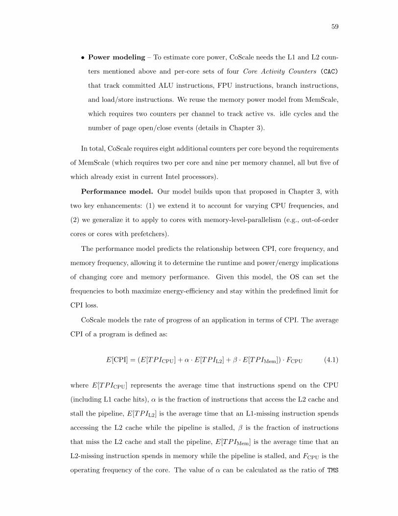
59
• Power modeling – To estimate core power, CoScale needs the L1 and L2 coun-
ters mentioned above and per-core sets of four Core Activity Counters (CAC)
that track committed ALU instructions, FPU instructions, branch instructions,
and load/store instructions. We reuse the memory power model from MemScale,
which requires two counters per channel to track active vs. idle cycles and the
number of page open/close events (details in Chapter 3).
In total, CoScale requires eight additional counters per core beyond the requirements
of MemScale (which requires two per core and nine per memory channel, all but five of
which already exist in current Intel processors).
Performance model. Our model builds upon that proposed in Chapter 3, with
two key enhancements: (1) we extend it to account for varying CPU frequencies, and
(2) we generalize it to apply to cores with memory-level-parallelism (e.g., out-of-order
cores or cores with prefetchers).
The performance model predicts the relationship between CPI, core frequency, and
memory frequency, allowing it to determine the runtime and power/energy implications
of changing core and memory performance. Given this model, the OS can set the
frequencies to both maximize energy-efficiency and stay within the predefined limit for
CPI loss.
CoScale models the rate of progress of an application in terms of CPI. The average
CPI of a program is defined as:
E[CPI] = (E[TPICPU] + α · E[TPIL2] + β · E[TPIMem]) · FCPU (4.1)
where E[TPICPU] represents the average time that instructions spend on the CPU
(including L1 cache hits), α is the fraction of instructions that access the L2 cache and
stall the pipeline, E[TPIL2] is the average time that an L1-missing instruction spends
accessing the L2 cache while the pipeline is stalled, β is the fraction of instructions
that miss the L2 cache and stall the pipeline, E[TPIMem] is the average time that an
L2-missing instruction spends in memory while the pipeline is stalled, and FCPU is the
operating frequency of the core. The value of α can be calculated as the ratio of TMS
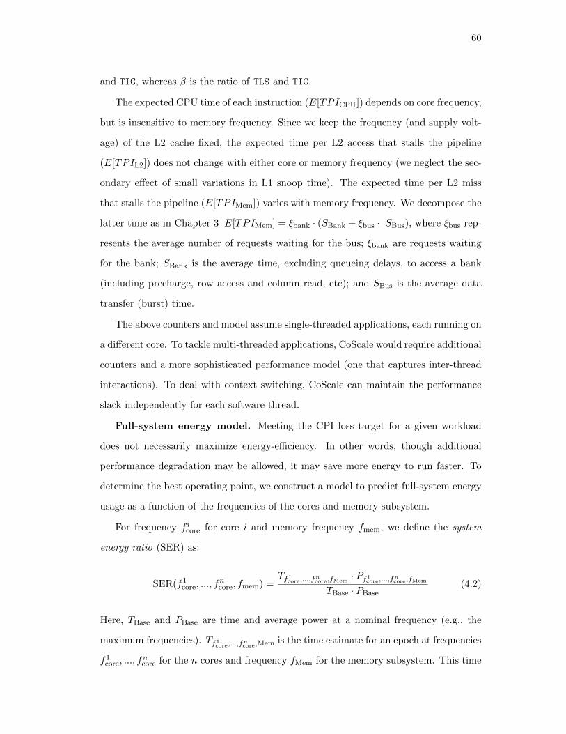
60
and TIC, whereas β is the ratio of TLS and TIC.
The expected CPU time of each instruction (E[TPICPU]) depends on core frequency,
but is insensitive to memory frequency. Since we keep the frequency (and supply volt-
age) of the L2 cache fixed, the expected time per L2 access that stalls the pipeline
(E[TPIL2]) does not change with either core or memory frequency (we neglect the sec-
ondary effect of small variations in L1 snoop time). The expected time per L2 miss
that stalls the pipeline (E[TPIMem]) varies with memory frequency. We decompose the
latter time as in Chapter 3 E[TPIMem] = ξbank · (SBank + ξbus · SBus), where ξbus rep-
resents the average number of requests waiting for the bus; ξbank are requests waiting
for the bank; SBank is the average time, excluding queueing delays, to access a bank
(including precharge, row access and column read, etc); and SBus is the average data
transfer (burst) time.
The above counters and model assume single-threaded applications, each running on
a different core. To tackle multi-threaded applications, CoScale would require additional
counters and a more sophisticated performance model (one that captures inter-thread
interactions). To deal with context switching, CoScale can maintain the performance
slack independently for each software thread.
Full-system energy model. Meeting the CPI loss target for a given workload
does not necessarily maximize energy-efficiency. In other words, though additional
performance degradation may be allowed, it may save more energy to run faster. To
determine the best operating point, we construct a model to predict full-system energy
usage as a function of the frequencies of the cores and memory subsystem.
For frequency f icore for core i and memory frequency fmem, we define the system
energy ratio (SER) as:
SER(f1core, ..., f
ncore, fmem) =
Tf1core,...,f
ncore,fMem
· Pf1core,...,f
ncore,fMem
TBase · PBase(4.2)
Here, TBase and PBase are time and average power at a nominal frequency (e.g., the
maximum frequencies). Tf1core,...,f
ncore,Mem is the time estimate for an epoch at frequencies
f1core, ..., f
ncore for the n cores and frequency fMem for the memory subsystem. This time

61
estimate corresponds to the core with the highest CPI degradation compared to running
at maximum frequency.
Pf1core,...,f
ncore,fMem
= PNonCoreL2OrMem + PL2+
PMem(fMem) +n∑
i=1
P iCore(f
icore).
(4.3)
In this formula, PNonCoreL2OrMem accounts for all system components other than the
cores, the shared L2 cache, and the memory subsystem, and is assumed to be fixed. PL2
is the average power of the L2 cache and is computed from its leakage and number of
accesses during the epoch. PMem(f) is the average power of L2 misses and is calculated
according to the model for memory power in [65]. We find that this average power does
not vary significantly with core frequency (roughly 1-2% in our simulations); workload
and memory bus frequency have a stronger impact. Thus, our power model assumes
that core frequency does not affect memory power. P iCore(f) is calculated based on the
cores’ activity factors using the same approach as prior work [11, 42]. We also find that
the power of the cores is essentially insensitive to the memory frequency.
4.2.4 Hardware and Software Costs
We now consider CoScale’s implementation cost. Core DVFS is widely available in com-
modity hardware, although each voltage domain may currently contain several cores.
Though CPUs with multiple frequency domains are common, there have historically
been few voltage domains; however, research has shown this is likely to change soon
[46, 89].
Our design also may require enhancements to performance counters in some proces-
sors. Most processors already expose a set of counters to observe processing, caching and
memory-related performance behaviors (e.g., row buffer hits/misses, row pre-charges).
In fact, Intel’s Nehalem architecture already exposes many MC counters for queues [52].
However, the existing counters may not conform precisely to the specifications required
for our models.

62
When CoScale adjusts the frequency of a component, the component briefly sus-
pends operation. However, as our policy operates at the granularity of multiple mil-
liseconds, and transition latencies are in the tens of microseconds, the overheads are
negligible. As mentioned above, the execution time of the search algorithm is not a
major concern.
Existing DIMMs support multiple frequencies and can switch among them by transi-
tioning to powerdown or self-refresh states [44], although this capability is typically not
used by current servers. Integrated CMOS MCs can leverage existing DVFS technology.
One needed change is for the MC to have separate voltage and frequency control from
other processor components. In recent Intel architectures, this would require separating
last-level cache and MC voltage control [40]. Although changing the voltage of DIMMs
and DRAM peripheral circuitry is possible [50], there are no commercial devices with
this capability.
4.3 Evaluation
We now present our methodology and results.
4.3.1 Methodology
Workloads. Table 4.1 describes the workload mixes we use. The mixes are similar to
those we used to evaluate MemScale in Chapter 3 (Table 3.1). The workload classes
are: memory-intensive (MEM), compute-intensive (ILP), compute-memory balanced
(MID), and a new mixed class (MIX, in which each workload embodies one or two
applications from each other class). We have replaced some old applications in the
MEM category to include more memory-intensive applications from SPEC 2006 suites.
The rightmost column of Table 4.1 lists the application composition of each workload;
four copies of each application are executed to occupy all 16 cores. Note that the MPKI
and WPKI values for these workloads are different than those in Table 3.1, because our
simulation of CoScale also had to include a detailed LLC module (described later in
this section).
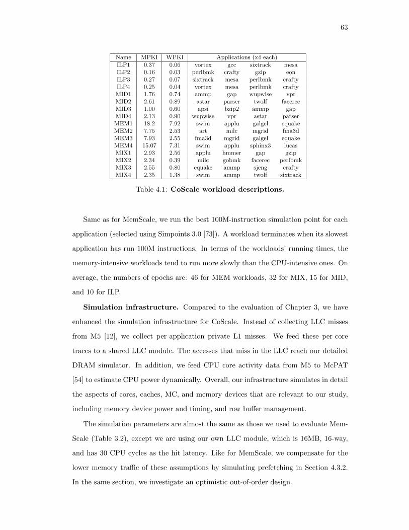
63
Name MPKI WPKI Applications (x4 each)
ILP1 0.37 0.06 vortex gcc sixtrack mesaILP2 0.16 0.03 perlbmk crafty gzip eonILP3 0.27 0.07 sixtrack mesa perlbmk craftyILP4 0.25 0.04 vortex mesa perlbmk craftyMID1 1.76 0.74 ammp gap wupwise vprMID2 2.61 0.89 astar parser twolf facerecMID3 1.00 0.60 apsi bzip2 ammp gapMID4 2.13 0.90 wupwise vpr astar parserMEM1 18.2 7.92 swim applu galgel equakeMEM2 7.75 2.53 art milc mgrid fma3dMEM3 7.93 2.55 fma3d mgrid galgel equakeMEM4 15.07 7.31 swim applu sphinx3 lucasMIX1 2.93 2.56 applu hmmer gap gzipMIX2 2.34 0.39 milc gobmk facerec perlbmkMIX3 2.55 0.80 equake ammp sjeng craftyMIX4 2.35 1.38 swim ammp twolf sixtrack
Table 4.1: CoScale workload descriptions.
Same as for MemScale, we run the best 100M-instruction simulation point for each
application (selected using Simpoints 3.0 [73]). A workload terminates when its slowest
application has run 100M instructions. In terms of the workloads’ running times, the
memory-intensive workloads tend to run more slowly than the CPU-intensive ones. On
average, the numbers of epochs are: 46 for MEM workloads, 32 for MIX, 15 for MID,
and 10 for ILP.
Simulation infrastructure. Compared to the evaluation of Chapter 3, we have
enhanced the simulation infrastructure for CoScale. Instead of collecting LLC misses
from M5 [12], we collect per-application private L1 misses. We feed these per-core
traces to a shared LLC module. The accesses that miss in the LLC reach our detailed
DRAM simulator. In addition, we feed CPU core activity data from M5 to McPAT
[54] to estimate CPU power dynamically. Overall, our infrastructure simulates in detail
the aspects of cores, caches, MC, and memory devices that are relevant to our study,
including memory device power and timing, and row buffer management.
The simulation parameters are almost the same as those we used to evaluate Mem-
Scale (Table 3.2), except we are using our own LLC module, which is 16MB, 16-way,
and has 30 CPU cycles as the hit latency. Like for MemScale, we compensate for the
lower memory traffic of these assumptions by simulating prefetching in Section 4.3.2.
In the same section, we investigate an optimistic out-of-order design.
64
We assume per-core DVFS, with 10 equally-spaced frequencies in the range 2.2-
4.0 GHz. We assume a voltage range matching Intel’s Sandybridge, from 0.65 V to
1.2 V, with voltage and frequency scaling proportionally, which matches the behavior
we measured on an i7 CPU. We assume uncore components, such as the shared LLC,
are always clocked at the nominal frequency and voltage. The memory system DVFS
configurations are the same as MemScale. In summary the frequencies of the memory
bus and the DRAM chips range from 800 MHz to 200 MHz, with steps of 66 MHz.
Transitions between bus frequencies are assumed to take 512 memory cycles plus 28 ns.
The register and MC power scale linearly with utilization, whereas PLL power scales
only with frequency and voltage. As a function of utilization, the PLL/register power
ranges from 0.1 W to 0.5 W [29, 39]. The MC power ranges from 4.5 W to 15 W,
slightly different than the evaluation in Chapter 3, to better reflect lower idle power on
the newer technology node.
We do not model power for non-CPU, non-memory system components in detail;
rather, we assume these components contribute a fixed 10% of the total system power
in the absence of energy management (we show the impact of varying this percentage
in Section 4.3.2).
Under our baseline assumptions, at maximum frequencies, the CPU accounts for
roughly 60%, the memory subsystem 30%, and other components 10% of system power.
4.3.2 Results
Energy and Performance
We first evaluate CoScale with a maximum allowable performance degradation of 10%.
We consider lower performance bounds in Section 4.3.2.
Figure 4.5 shows the full-system, memory, and CPU energy savings CoScale achieves
for each workload, compared to a baseline without energy management (i.e., maximum
frequencies). The memory energy savings range from -0.5% to 57% and the CPU energy
savings range from 16% to 40%. As one would expect, the ILP workloads achieve the
highest memory and lowest CPU energy savings, but still save at least 21% system

65
-10%
0%
10%
20%
30%
40%
50%
60%
MEM
1
MEM
2
MEM
3
MEM
4
MID1
MID2
MID3
MID4
ILP1
ILP2
ILP3
ILP4
MIX1
MIX2
MIX3
MIX4
AVG
Ene
rgy
Savi
ngs
(%
)
Fullsystemenergy Memoryenergy CPUenergy
Figure 4.5: CoScale energy savings. CoScale conserves up to 24% of the full-system energy.
0%
2%
4%
6%
8%
10%
12%
MEM
1M
EM2
MEM
3
MEM
4M
ID1
MID
2M
ID3
MID
4
ILP
1IL
P2
ILP
3IL
P4
MIX
1
MIX
2M
IX3
MIX
4A
VG
Pe
rf. D
egr
adat
ion
(%
)
Multiprogram average Worst program in mix
Perf. degradation bound
Figure 4.6: CoScale performance. CoScale never violates the 10% performance bound.
energy.
The memory energy savings in the MID and MIX workloads are lower but still sig-
nificant, whereas the CPU energy savings are somewhat higher (system energy savings
of at least 13% for both workload classes). Note that CoScale is successful at picking
the right energy saving “knob” in the MIX workloads. Specifically, it more aggressively
conserves memory energy in MIX3, whereas it more aggressively conserves CPU energy
in MIX1, MIX2, and MIX4.
The MEM workloads achieve the smallest memory and largest CPU energy savings
(system energy savings of at least 12%), since their greater memory channel traffic
reduces the opportunities for memory subsystem DVFS.
Figure 4.6 shows the average and maximum percent performance losses relative to
the maximum-frequency baseline. The figure shows that CoScale never violates the
performance bound. Moreover, CoScale translates nearly all the performance slack into
energy savings, with an average performance loss of 9.6%, quite near the 10% target.

66
2
2.5
3
3.5
4
4.5
0.2
0.3
0.4
0.5
0.6
0.7
0.8
0.9
1 3 5 7 9 11 13 15 17 19 21 23 25
Co
re f
req
ue
ncy
(G
Hz)
Me
m. f
req
ue
ncy
(G
Hz)
(a) CoScale
memory frequency core frequency
2
2.5
3
3.5
4
4.5
0.2
0.3
0.4
0.5
0.6
0.7
0.8
0.9
1 3 5 7 9 11 13 15 17 19 21 23 25
Co
re f
req
ue
ncy
(G
Hz)
Me
m. f
req
ue
ncy
(G
Hz)
(c) Semi-Coordinated
2
2.5
3
3.5
4
4.5
0.2
0.3
0.4
0.5
0.6
0.7
0.8
0.9
1 3 5 7 9 11 13 15 17 19 21 23 25
Co
re f
req
ue
ncy
(G
Hz)
Me
m. f
req
ue
ncy
(G
Hz)
(b) Uncoordinated
Figure 4.7: Timeline of the milc application in MIX2. Milc exhibits three phases.CoScale adjusts core and memory subsystem frequency precisely and rapidly in response to thephase changes. The other techniques do not.
In summary, CoScale conserves between 13% and 24% full-system energy for a wide
range of workloads, always within the user-defined performance bounds.
Dynamic Behavior
To provide greater insight, we study an example of the dynamic behavior of CoScale
in detail. Figure 4.7 plots the memory subsystem and core frequency (for milc in
MIX2) selected by CoScale over time. For comparison, we also show the behavior of
the Uncoordinated and Semi-coordinated policies.
Figure 4.7(a) shows that, in epoch two, CoScale reduces the core and memory
frequencies to consume the available slack. In this phase, milc has low memory traffic
needs, but the other applications in the mix preclude lowering the memory frequency
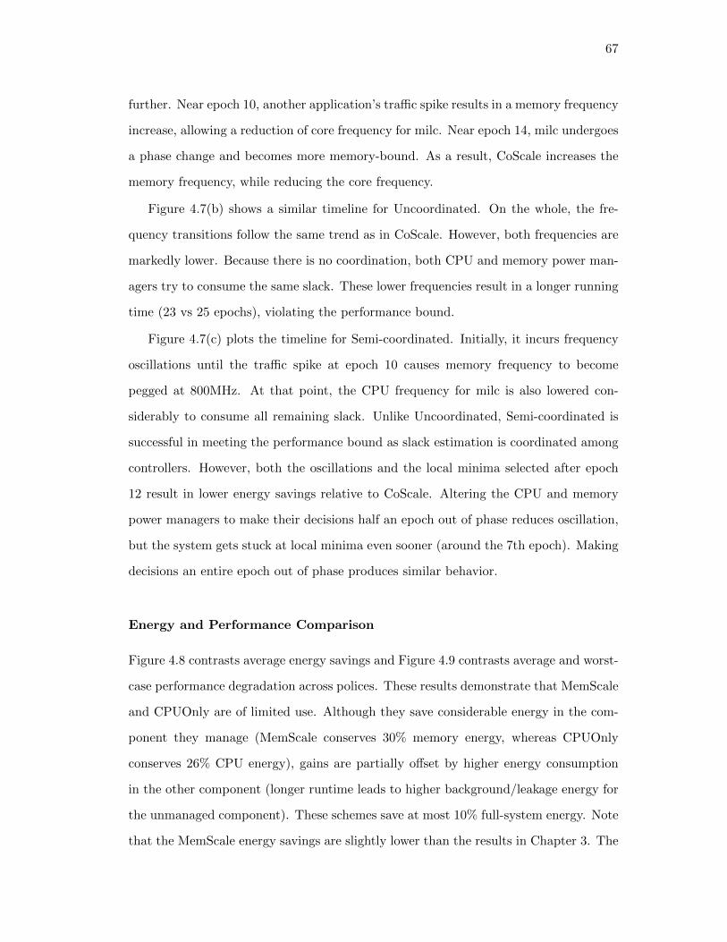
67
further. Near epoch 10, another application’s traffic spike results in a memory frequency
increase, allowing a reduction of core frequency for milc. Near epoch 14, milc undergoes
a phase change and becomes more memory-bound. As a result, CoScale increases the
memory frequency, while reducing the core frequency.
Figure 4.7(b) shows a similar timeline for Uncoordinated. On the whole, the fre-
quency transitions follow the same trend as in CoScale. However, both frequencies are
markedly lower. Because there is no coordination, both CPU and memory power man-
agers try to consume the same slack. These lower frequencies result in a longer running
time (23 vs 25 epochs), violating the performance bound.
Figure 4.7(c) plots the timeline for Semi-coordinated. Initially, it incurs frequency
oscillations until the traffic spike at epoch 10 causes memory frequency to become
pegged at 800MHz. At that point, the CPU frequency for milc is also lowered con-
siderably to consume all remaining slack. Unlike Uncoordinated, Semi-coordinated is
successful in meeting the performance bound as slack estimation is coordinated among
controllers. However, both the oscillations and the local minima selected after epoch
12 result in lower energy savings relative to CoScale. Altering the CPU and memory
power managers to make their decisions half an epoch out of phase reduces oscillation,
but the system gets stuck at local minima even sooner (around the 7th epoch). Making
decisions an entire epoch out of phase produces similar behavior.
Energy and Performance Comparison
Figure 4.8 contrasts average energy savings and Figure 4.9 contrasts average and worst-
case performance degradation across polices. These results demonstrate that MemScale
and CPUOnly are of limited use. Although they save considerable energy in the com-
ponent they manage (MemScale conserves 30% memory energy, whereas CPUOnly
conserves 26% CPU energy), gains are partially offset by higher energy consumption
in the other component (longer runtime leads to higher background/leakage energy for
the unmanaged component). These schemes save at most 10% full-system energy. Note
that the MemScale energy savings are slightly lower than the results in Chapter 3. The

68
-10%
0%
10%
20%
30%
Ene
rgy
Savi
ngs
(%
)
Full system energy Memory system energy CPU energy
Figure 4.8: Energy savings. CoScale provides greater full-system energy savings thanthe practical policies.
main reason is that in this chapter we use McPAT to estimate CPU power accurately,
whereas in Chapter 3 we assume a fixed rest-of-system (including CPU) power con-
sumption. This change also causes the memory power to represent a smaller fraction
of the full-system power.
Uncoordinated conserves substantial memory and CPU energy, achieving the high-
est full-system energy savings of any scheme. Unfortunately, it is incapable of keeping
the performance loss under the pre-defined 10% bound. In some cases, the perfor-
mance degradation reaches 19%, nearly twice the bound. On the other hand, Semi-
coordinated bounds performance well because the managers share the slack estimate.
However, because of frequent oscillations and settling at sub-optimal local minima,
Semi-coordinated consumes up to 8% more system energy (2.6% on average) than
CoScale. Reducing oscillations by having the power managers make decisions out of
phase does not improve results (0.3% lower savings with the same performance).
CoScale is more stable and effective than the other practical policies at conserving
both memory and CPU energy, while staying within the performance bound. CoScale
does almost as well as Offline. These results show that our heuristic for selecting
frequencies is almost as effective as considering an exponential number of possibilities
with prior knowledge of each workload’s behavior.

69
0%
5%
10%
15%
20%
Pe
rf. D
egr
adat
ion
s (%
)
Multiprogram Average Worst in Mix
Perf.degradation bound
Figure 4.9: Performance. Uncoordinated is incapable of limiting performance degra-dation.
Sensitivity Analysis
To illustrate CoScale’s behavior across different system and policy settings, we report on
several sensitivity studies. In every case, we vary a single parameter at a time, leaving
the others at their default values. Given the large number of potential experiments, we
usually present results only for the MID workloads, which are sensitive to both memory
and core performance.
Acceptable performance loss. In Figure 4.10, we vary the maximum allowable
performance degradation, showing energy savings. Recall that our other experiments
use a bound of 10%. As one would expect, 1% and 5% bounds produce lower energy
savings, averaging 4% and 9%, respectively. Allowing 15% and 20% degradations saves
more energy. In all cases, CoScale meets the configured bound, and provides greater
percent energy savings than performance loss, even for tight performance bounds.
Rest-of-the-system power consumption. Figure 4.11 illustrates the effect of
doubling and halving our assumption for non-memory, non-core power. When this
power is doubled, CoScale still achieves 14% average full-system energy savings, whereas
the savings increase to 17% when it is halved. In all cases performance remains within
bounds (not shown).
Ratio of memory subsystem and CPU power. We also consider the effect of
varying the ratio of memory subsystem to CPU power. Recall that, under our baseline
power assumptions, CPU accounts for 60%, while memory accounts for 30% of total

70
0%
10%
20%
30%
Ener
gy S
avin
gs (
%)
1% Bound 5% Bound10% Bound 15% Bound20% Bound
Figure 4.10: Impact of performancebound. Higher bound allows more sav-ings without violations.
0%
5%
10%
15%
20%
Ener
gy S
avin
gs (
%)
5% Other 10% Other
15% Other 20% Other
Figure 4.11: Impact of rest-of-systempower. Savings still high for higher rest-of-system power.
0%
5%
10%
15%
20%
25%
Ener
gy S
avin
gs (
%)
CPU:Mem-2:1CPU:Mem-1:1CPU:Mem-1:2
Figure 4.12: Impact of CPU:mempower, MID. Savings increase as mem-ory power increases.
0%
5%
10%
15%
Ener
gy S
avin
gs (
%)
CPU:Mem-2:1CPU:Mem-1:1CPU:Mem-1:2
Figure 4.13: Impact of CPU:mempower, MEM. Savings decrease as mem-ory power increases.
power at peak frequency (a CPU:Mem ration of 2:1). In Figure 4.12, we consider 1:1
and 1:2 ratios. CoScale achieves greater energy savings when the fraction of memory
power is higher for the MID workloads. Interestingly, this trend is reversed for our
MEM workloads (Figure 4.13), as most savings come from scaling the CPU.
CPU voltage range. We next consider the impact of a narrower CPU (and
MC) voltage range, which reduces CoScale’s ability to conserve core energy. Figure
4.14 shows results for a half-width range (0.95 1.2v) relative to our default assumption
(0.65 1.2v). When the marginal utility of lowering CPU frequency decreases, CoScale
scales the memory subsystem more aggressively and still achieves 11% full-system en-
ergy savings on average.
Number of available frequencies. By default, we assume 10 frequencies for both
the CPU and the memory subsystem. Figure 4.15 shows results for 4 and 7 frequencies
as well. As expected, the energy savings decrease as the granularity becomes coarser.

71
0%
5%
10%
15%
20%
Ener
gy S
avin
gs (
%)
Half CPU Vol. Range
Full CPU Vol. Range
Figure 4.14: Impact of CPU voltagerange. Smaller voltage ranges reduce en-ergy savings.
0%
5%
10%
15%
20%
Ener
gy S
avin
gs (
%)
4 Freqs 7 Freqs
10 Freqs
Figure 4.15: Impact of number of fre-quencies. Savings decrease little whenfewer steps are avalaible.
0%
20%
40%
60%
80%
100%
120%
MEM MID ILP MIX
Ene
rgy
pe
r in
str.
(N
orm
.)
Base Base+Pref.
Base+CoScale Base+Pref.+CoScale
Figure 4.16: Impact of prefetching. CoScale works well with and without prefetch-ing.
However, CoScale adapts well, conserving only slightly less energy with fewer frequen-
cies. With 4 frequencies the maximum performance loss is slightly lower than 10%,
because the coarser granularity limits CoScale’s ability to consume the slack precisely.
Prefetching. Next, we consider the impact of the increase in memory traffic that
arises from prefetching. We implement a simple next-line prefetcher. This prefetcher
is effective for these workloads, always decreasing the LLC miss rate. However, the
prefetcher is not perfect; its accuracy ranges from 52% to 98% across our workloads.
On average, it improves performance by almost 20% on MEM workloads, 8% on MIX,
4% on MID, and 1% for ILP. At the same time, it increases the memory traffic more
than 33% on MEM, 20% on MID, 33% on MIX, and 13% on ILP. As one might expect,
the higher memory traffic and instruction throughput result in higher memory and CPU
power.
Figure 4.16 shows the full-system energy per instruction of three designs (Base+prefetching,
Base+CoScale, and Base+prefetching+CoScale) normalized to our baseline (Base). We

72
can see that the energy consumptions of Base+prefetching and Base are almost the
same, except for the MEM workloads, since higher power and better performance
roughly balance from an energy-efficiency perspective. Again except for MEM, the
energy consumptions of Base+CoScale and Base+prefetching+CoScale are almost ex-
actly the same, since average memory frequency is lower but CPU frequency is higher.
For the MEM workloads, the performance improvement due to prefetching dominates
the average power increase, so the average energy of Base+prefetching is 7% lower than
Base. In addition, Base+prefetching+CoScale achieves 17% energy savings, compared
to 12% from Base+CoScale. These results show that CoScale works well both with and
without prefetching.
Out-of-Order. Although our trace-based methodology does not allow detailed
out-of-order (OoO) modeling, we can approximate the latency hiding and additional
memory pressure of OoO by emulating an instruction window during trace replay. We
make the simplifying assumption that all memory operations within any 128-instruction
window are independent, thereby modeling an upper bound on memory-level parallelism
(MLP). Note that we still model a single-issue pipeline, hence, our instruction window
creates MLP, but has no impact on instruction-level parallelism. Figure 4.17 compares
the average CPI of the in-order and OoO designs, with and without CoScale, normalized
to the in-order result. At one extreme, OoO drastically improves MEM, as memory
stalls can frequently overlap. At the other extreme, ILP gains no benefit, since the
infrequent L2 misses do not overlap frequently enough to impact performance. Note
that, in the OoO+CoScale cases, performance remains within 10% of the OoO case;
that is, CoScale is still maintaining the target degradation bound. Although we do
not show these results in the figure, similar to the in-order case, Semi-coordinated on
OoO meets the performance requirement, whereas Uncoordinated on OoO does not –
Uncoordinated on OoO degrades performance by up to 16%, on a 10% performance
loss bound.
Figure 4.18 shows average energy per instruction normalized to In-order. As we do
not model any power overhead for OoO hardware structures (only the effects of higher
instruction throughput and memory traffic), OoO always breaks even (ILP and MIX)
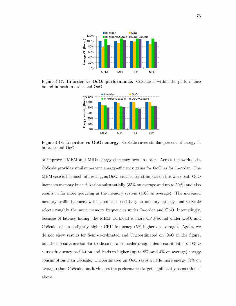
73
0%
20%
40%
60%
80%
100%
120%
MEM MID ILP MIX
Ave
rage
CP
I (N
orm
.)
In-order OoO
In-order+CoScale OoO+CoScale
Figure 4.17: In-order vs OoO: performance. CoScale is within the performancebound in both in-order and OoO.
0%
20%
40%
60%
80%
100%
120%
MEM MID ILP MIX
Ene
rgy
pe
r in
str.
(N
orm
.)
In-order OoO
In-order+CoScale OoO+CoScale
Figure 4.18: In-order vs OoO: energy. CoScale saves similar percent of energy inin-order and OoO.
or improves (MEM and MID) energy efficiency over In-order. Across the workloads,
CoScale provides similar percent energy-efficiency gains for OoO as for In-order. The
MEM case is the most interesting, as OoO has the largest impact on this workload. OoO
increases memory bus utilization substantially (35% on average and up to 50%) and also
results in far more queueing in the memory system (43% on average). The increased
memory traffic balances with a reduced sensitivity to memory latency, and CoScale
selects roughly the same memory frequencies under In-order and OoO. Interestingly,
because of latency hiding, the MEM workload is more CPU-bound under OoO, and
CoScale selects a slightly higher CPU frequency (5% higher on average). Again, we
do not show results for Semi-coordinated and Uncoordinated on OoO in the figure,
but their results are similar to those on an in-order design. Semi-coordinated on OoO
causes frequency oscillation and leads to higher (up to 8%, and 4% on average) energy
consumption than CoScale. Uncoordinated on OoO saves a little more energy (1% on
average) than CoScale, but it violates the performance target significantly as mentioned
above.

74
Summary. These sensitivity studies demonstrate that CoScale’s performance mod-
eling and control frameworks are robust—across the parameter space, CoScale always
meets the target performance bound, while energy savings vary in line with expecta-
tions. Although the results in this subsection focused mostly on the MID workloads,
we observed similar trends with the other workloads as well.
4.4 Conclusion
In this chapter, we proposed CoScale, a hardware-software approach for managing CPU
and memory subsystem energy (via DVFS) in a coordinated fashion, under performance
constraints. Our evaluation showed that CoScale conserves significant CPU, memory,
and full-system energy, while staying within the performance bounds; that it is superior
to four competing energy management techniques; and that it is robust over a wide
parameter space. We conclude that CoScale’s potential benefits far outweigh its small
hardware costs.
75
Chapter 5
MultiScale
5.1 Introduction
Previous chapters have shown that the active low-power modes for main memory are
good at trading memory performance for energy savings. However, they only select
a single performance setting for the memory system and are thus ideal for systems
with a single MC. On the other hand, chip multiprocessors are increasingly integrating
multiple on-die MCs [1, 6, 87]. Furthermore, recent work has demonstrated the benefit
of deliberately skewing traffic across multiple MCs to preserve fair performance among
applications judged likely to interfere (i.e., by placing data such that memory-intensive
and non-memory intensive applications access disjoint MCs/channels) [68]. Such asym-
metric traffic patterns will call for correspondingly asymmetric DVFS control.
Recent hardware trends also suggest that traffic skew across MCs will grow. For
example, as servers increasingly rely on multi-socket configurations, inter-socket MC
bandwidth requirements will vary significantly [86]. In addition, the advent of het-
erogeneous processors incorporating sophisticated superscalar out-of-order cores with
simpler in-order cores (e.g., ARM’s big.LITTLE architecture [30]), and graphics pro-
cessing units (e.g., AMD’s Fusion and Intel’s Sandybridge architectures [79]), will fun-
damentally increase traffic skew across MCs. Therefore, it is critical to explore novel
multi-MC active low-power mode management techniques. The straight-forward ex-
tension of prior work—selecting the same frequency for all MCs based on their average
bandwidth requirement—will lead to sub-optimal savings under skewed traffic.
Thus, this chapter presents MultiScale, a set of software policies and hardware
mechanisms for coordinating DVFS across multiple MCs, channels, and devices. Un-
der OS control, MultiScale monitors per-application traffic across MCs and estimates
76
their varying bandwidth and latency requirements. It then uses a heuristic algorithm
to quickly select and apply an optimized MC frequency combination. Same as Mem-
Scale and CoScale, MultiScale’s goal is to minimize the overall system energy, without
degrading performance beyond a user-specified limit. Unlike past work however, Multi-
Scale is able to do so effectively and consistently for multi-MC systems under a variety
of traffic skews.
We evaluate MultiScale using detailed simulation on a diverse set of workload mixes
constructed from the SPEC benchmark suite [81]. We quantify MultiScale’s benefits
across a range of traffic-skew patterns, showcasing its consistently higher energy effi-
ciency versus MemScale.
This work is the first to study techniques to apply memory system active low-
power modes to multiple MCs in a coordinated manner. First, we develop a set of
low-overhead, yet effective software policies and hardware mechanisms that monitor
per-application, per-MC bandwidth/latency requirements. Our readily-implementable
performance counters, allied with low-overhead OS support, can be used to realize Mul-
tiScale’s performance and energy models. Second, we quantify MultiScale’s ability to
exploit user-defined per-application performance degradation constraints across a range
of traffic skew patterns. Our results show that MultiScale’s ability to coordinate per-
MC DVFS based on the workloads’ dynamic memory bandwidth requirements allows it
to achieve up to 4.5 times greater energy savings than prior approaches. MultiScale is
effective even in situations when performance constraints are tight; for example, when
the allowable degradation is capped at just 1%, MultiScale can still achieve energy
savings over 9% whereas past work achieves savings of merely 2%.
The remainder of the chapter is structured as follows. We present background and
motivation in the next section. Section 5.3 describes MultiScale in detail. Section 5.4
describes our evaluation methodology and results. Finally, Section 5.5 concludes the
chapter.

77
App A performance
App B performance
MC 0 frequency
MC 1 frequency
Perf. target:10% lower IPC
Perf. target:10% lower IPC
Perf. target:1% lower IPC
Perf. target:1% lower IPC
Profiling
(a) MemScale (b) MultiScale
Time
Profiling
Figure 5.1: Because it independently manages each MC, MultiScale can selecta lower frequency for MC 0 and thus save more energy than MemScale whileremaining within the prescribed performance bounds.
5.2 Motivation
MemScale selects a single performance setting for the memory system based on aggre-
gate application requirements. As such, it is unable to exploit time-varying or asym-
metric traffic patterns across MCs in multiple-MC systems. Figure 5.1 illustrates a
scenario where two applications, A and B, run on a dual-MC system. Suppose the
memory allocation is skewed such that 80% of application A’s accesses are directed to
MC 1, whereas application B’s accesses are predominantly to MC 0. Further, suppose
that application A is under a tight performance constraint, and can tolerate only a 1%
degradation, whereas application B can tolerate up to 10% slowdown. Application A’s
tight performance constraint will require MC 1 at a high frequency. However, there
might be substantial opportunity to slow MC 2 without violating the performance con-
straint of either application. MemScale (Figure 5.1 left) selects only a single frequency
for both MCs, based on the tighter performance constraint of application A, limiting
energy savings. In contrast, MultiScale (Figure 5.1 right) independently assesses the
bandwidth requirements of each MC and selects an appropriate frequency/voltage to
maximize energy savings while respecting each applications’ degradation constraint.
While the OS maps virtual to physical addresses, the interleaving of physical ad-
dresses has the greatest impact on the traffic skew across MCs. Cache line and page
interleaving seek to distribute traffic evenly. While such interleaving balances traffic
across MCs, there are many strong arguments and hardware/software trends pointing
78
toward addressing schemes that skew traffic across channels. For example, recent work
by Muralidhara and co-authors has demonstrated the benefit of deliberately skewing
traffic across multiple MCs to preserve fair performance among applications judged
likely to interfere [68]. Under this scheme, data from memory-intensive and non-
memory-intensive applications are mapped to disjoint MCs/channels. This isolates
non-memory-intensive workloads from interference effects of intense memory traffic,
while clever scheduling techniques manage access among the memory-intensive work-
loads. Similarly, Awasthi and co-authors propose mechanisms to place data in multi-MC
systems to improve performance [6]. Their approach, which balances the benefits of al-
locating application data to the MC closest to the corresponding core against queuing
delays, on-chip latencies, and row buffer hit rates, often results in traffic skew. Traffic
skew is also common in heterogeneous platforms with accelerators, such as graphics pro-
cessing units and sophisticated out-of-order cores coupled with simpler in-order cores,
which might impose differing bandwidth requirements across MCs.
MultiScale adapts better than MemScale to traffic skew across MCs. So, in char-
acterizing MultiScale, we have two primary goals: (1) We demonstrate its effectiveness
across a range of traffic patterns. To this end, we quantify MultiScale’s operation across
a spectrum of traffic skews. (2) We aim to showcase MultiScale’s effectiveness at real-
izing energy savings even under the tightest performance degradation constraints. To
this end, we study the benefits of MultiScale across a range of degradation constraints,
as small as 1% allowable slowdown.
5.3 MultiScale Design
MultiScale seeks to maximize energy savings while adhering to per-application user-
specified performance degradation constraints. We now detail the hardware mechanisms
and software policies that make this possible.

79
5.3.1 Hardware and Software
Hardware mechanisms. For each MC, MemScale adjusts its frequency and voltage
and the frequency of its associated memory channels and DIMMs; for expediency, we
shall refer to these operations collectively as “adjusting the MC frequency”. The DIMM
clocks lock to the bus frequency (or a multiple thereof), while the MC frequency is fixed
at double the bus frequency. While MultiScale can readily be applied to systems where
each MC controls multiple channels at different frequencies, assessing the hardware
overheads of such an approach is beyond the scope of this work. We therefore treat
each MC, together with all its memory channels, as the unit for frequency selection. A
frequency change requires the system to briefly suspend operation and reconfigure to
run at the new target. Our experiments model the associated recalibration delays.
Similar to MemScale and CoScale, MultiScale frequency scales the MCs, buses, and
DIMMs. Voltage scaling is restricted to the MCs, and is set according to the selected
frequencies.
Performance counter monitoring. Our management policies require input from
a set of performance counters implemented on each core and on-chip MC. Specifically,
we require counters tracking the amount of work pending at each MC’s memory banks
and channels. Counters similar to those we require already exist in most modern archi-
tectures, and are accessible through the CPU’s performance-monitoring interface. For
further details on the exact performance counters used, we refer the reader to Chapter
3 as MultiScale uses identical counters.
Energy management policy. Our goal is to minimize overall system energy con-
sumption without degrading performance beyond user-specified bounds. Therefore, as
in MemScale, MultiScale exploits the notion of performance slack: the difference be-
tween a baseline execution and a target slowdown that the each application may incur
to save energy. Our control algorithm exploits this allowable slack to reduce memory
system performance and save energy. The per-application performance target is de-
fined such that the application incurs no more than a pre-selected maximum slowdown
relative to its execution without energy management (i.e., at maximum frequency).
80
Formally, the slack is the difference in time of the program’s execution (TActual) from
the target (TTarget).
Slack = TTarget − TActual
= TMaxFreq · (1 + γ)− TActual
(5.1)
where γ defines the target maximal execution time increase.
In exploiting this slack, MultiScale’s control algorithm divides execution into fixed-
sized epochs. We typically associate an epoch with an OS time quantum. MultiScale
splits each epoch into four distinct phases. First, applications are profiled by collecting
statistics from the performance counters. We find that profiling for 300 µs in an epoch
of 5 ms suffices. Second, the OS uses the profiling information to select new MC
frequencies (as detailed in the next subsection). Third, each MC, its channels, and
DRAM devices are transitioned to their new frequency. Finally, the epoch completes at
this new frequency configuration. At the end of the epoch, we again query the counters
and estimate the performance that would have been achieved had the memory system
operated at maximum frequency. The difference between this estimate and the achieved
performance is used to update the slack and is carried forward to calculate the target
performance in the next epoch.
5.3.2 Performance and Energy Models
Performance model. Our control algorithm utilizes a performance model extended
from MemScale to account for per-MC frequencies and the traffic directed by each
application to each MC. The performance model predicts the relationship between
CPU CPI of an application, and the per-MC frequency. There are three steps in
our modeling approach. First, we estimate the memory-boundedness of each running
application, and thus estimate the target access latency that satisfies the performance
target of each application. Second, we estimate each MC’s contribution to this average
latency (which requires the MCs to be aware of the hardware thread that issued each
access). Finally, based on the first two steps, we calculate per-MC frequencies. Next,

81
we detail each step.
Step 1: Under our performance model, the runtime of a program is defined as: ttotal =
tCPU + tMem = ICPU ·E[TPICPU] + IMem ·E[LMem], where ICPU represents the number
of instructions, and Imem is the number of last-level cache (LLC) misses stalling the
pipeline. TPICPU represents the average time that instructions spend on the CPU (in-
cluding L1 cache hits, L1 cache misses, and L2 cache hits in a two-level cache hierarchy),
and LMem is the average memory latency of each application.
Since runtime is not known a priori, we model the rate of progress of an application
in terms of CPI. The average CPI of a program is defined as: E[CPI] = (E[TPICPU] +
α ·E[LMem]) ·FCPU, where α is the fraction of instructions that miss in the L2 cache and
stall the pipeline, and FCPU is the operating frequency of the core. The value of α can
easily be calculated as the ratio of instruction to LLC miss counts, accessible through
performance counters. Given a target CPI, we can compute E[LMem] assuming other
components in the above equation are constant. By substituting α into the equation and
dividing by the frequency, we can compute the target average per-application latency
needed to compute per-MC latency.
Step 2: Having calculated the target average memory access latency per application,
we now focus on the latency breakdown per MC. To understand this, consider a simple
scenario where there are two applications, A and B, and two MCs, MC 0 and MC 1.
Suppose that for A, PercA0% of total memory accesses go to channels under MC 0,
while PercA1% go to channels under MC 1. Further, assume that PercB0% of accesses
from B go to channels under MC 0, and PercB1% of accesses go to channels under
MC 1. We have: PercA0% + PercA1% = 100%
PercB0% + PercB1% = 100%
(5.2)
Assume that the average access latency to channels under MC 0 is L0, and to channels
under MC 1 is L1. Furthermore, denote the average memory access latency of A and

82
B is E[LA] and E[LB], respectively. We then have:
E[LA] = PercA0 · L0 + PercA1 · L1
E[LB] = PercB0 · L0 + PercB1 · L1
(5.3)
We can now use these equalities to calculate per-MC memory access latencies. Using
the information from step (1) on each application’s E[LMem], we can cap each applica-
tion’s latencies so as to ensure the correct performance targets. Specifically, assuming
that LTarget A and LTarget B are the threshold latencies that guarantee the performance
targets of A and B, we have the following inequalities.
E[LA] ≤ LTarget A
E[LB] ≤ LTarget B
(5.4)
Solving this system provides L0 and L1 values which can then be used as input to our
next step.
Although this simple example assumes two applications and two MCs, this approach
can be generalized to any number of applications and MCs. In general, this entails
solving a linear programming (LP) problem where the number of MCs is likely smaller
than the number of running applications. (MultiScale only needs to deal with the
applications running during the next epoch.) Standard LP solvers can be used to
calculate these latencies efficiently. The overhead of this computation is negligible for
realistic numbers of MCs, since it only occurs once per epoch. For our setup (4 MCs
and 16 cores), the overhead is less than 50 µs on a Xeon 5520 machine.
Step 3: Having solved for L0 and L1 and the latencies of all other MCs (which we
collectively denote as LMem), we model the relationship between channel frequency
and memory access latency. We take the approach of MemScale: E[LMem] = ξbank ·
(SBank + ξbus · SBus), where ξbus represents the average number of requests waiting for
the bus and is approximated by the counters capturing the queuing impact of waiting
for bus transfers; ξbank represents the average number of requests waiting for the bank
and is approximated by the counters capturing per bank queuing; SBank is the average
83
time, excluding queueing delays, to access a bank (including precharge, row access and
column read, etc); and SBus is the average data transfer (burst) time across the bus.
Since the values of SBank, ξbank, and ξbus can be obtained by profiling performance
counters, we can calculate SBus, which is a function of the frequency. Finally, we can
calculate the target frequency from SBus.
Full-system energy model. Simply meeting the CPI loss target for a given work-
load does not necessarily maximize energy efficiency. In other words, though additional
performance degradation may be allowed, it may save more energy to run faster. To
determine the best operating point, we construct a model to predict full-system energy
usage. For memory frequency fMC 1,fMC 2, ..., fMC N, we define the system energy ratio
(SER) as:
SER(fmem) =TfMem
· (∑
i PfMC i+ PNonMem)
TBase · PBase(5.5)
TfMemis the performance estimate for an epoch at frequency fMC 1 through fMC N.
Memory power is calculated with the memory power model in [65], and PNonMem ac-
counts for all non-memory system components and is assumed to be fixed. TBase and
PBase are corresponding values at a nominal frequency. At the end of each epoch’s
profiling phase, we calculate SER for all memory frequencies that can meet the perfor-
mance constraint given by the slack, and select the frequency that minimizes the SER,
from the range calculated by the latency model as described earlier in this section.
5.4 Evaluation
In this section, we demonstrate the efficacy of MultiScale over a range of traffic skews
relative to MemScale.
5.4.1 Methodology
Simulator and workloads. Our evaluations are based on a two-step simulation
methodology similar to ones in Chapter 3 and Chapter 4. The only difference is that
we are modeling 4 MCs, where each MC can be set at a different frequency and voltage.
Each MC’s power ranges from 2W to 4W, depending on the voltage, frequency, and

84
Name MPKI WPKI Applications (x4 each)MIX1 2.93 2.56 applu hmmer gap gzipMIX2 2.34 0.39 milc gobmk facerec perlbmkMIX3 2.55 0.80 equake ammp sjeng craftyMIX4 2.41 1.41 lucas vpr h264ref eonMIX5 2.35 1.38 swim ammp twolf sixtrackMIX6 2.91 1.57 libquantum twolf vpr sjengMIX7 3.12 1.48 mcf astar gzip sixtrackMIX8 1.83 0.77 mgrid fma3d crafty eon
Table 5.1: MultiScale workload descriptions.
utilization. Based on these values, our memory system (including MCs) accounts for
44% of the total system power on average. We further assume the 16 cores are inter-
connected using as 4x4 mesh with the MCs on the corners. Every set of 4 cores has a
local MC, which is at the adjacent corner.
Table 5.1 lists the main characteristics of our 8 workloads. Those workloads are
different than those in Chapter 3 and Chapter 4. We are using all MIX workloads which
can better represent the traffic interference pattern studied in [68]. The workloads are
formed by combining applications from the SPEC 2000 and SPEC 2006 suites. We
analyze the best 100M-instruction simulation point for each application (selected using
Simpoints 3.0 [73]). The workload terminates when the slowest application has executed
100M instructions.
Experiments. We compare MultiScale to MemScale for different traffic distribu-
tions and performance degradation bounds. We distribute traffic by controlling how
many pages of each application are allocated to its local MC. In our experiments, we
vary this from 100% (the extreme form of channel partitioning proposed in [68]) to
80%, 60%, 40%, 25%, and 20%. Non-local MC pages are allocated randomly across
the remote MCs. Thus, the 25% case represents the scenario in which each MC is
responsible for (roughly) the same number of pages.
For each of these cases, we investigate 1%, 3%, 5%, 7%, and 10% allowable perfor-
mance slowdowns.
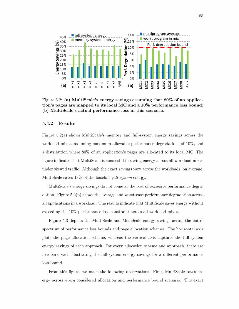
85
0%5%
10%15%20%25%30%35%40%45%
MIX
1
MIX
2
MIX
3
MIX
4
MIX
5
MIX
6
MIX
7
MIX
8
AV
G
Ene
rgy
Savi
ngs
(%
)
fullsystemenergymemorysystemenergy
0%
2%
4%
6%
8%
10%
12%
14%
MIX
1
MIX
2
MIX
3
MIX
4
MIX
5
MIX
6
MIX
7
MIX
8
AV
G
Per
f. D
egra
dat
ion
(%
)
multiprogram averageworst program in mix
Perf. degradation bound
(a) (b)
Figure 5.2: (a) MultiScale’s energy savings assuming that 80% of an applica-tion’s pages are mapped to its local MC and a 10% performance loss bound;(b) MultiScale’s actual performance loss in this scenario.
5.4.2 Results
Figure 5.2(a) shows MultiScale’s memory and full-system energy savings across the
workload mixes, assuming maximum allowable performance degradations of 10%, and
a distribution where 80% of an application’s pages are allocated to its local MC. The
figure indicates that MultiScale is successful in saving energy across all workload mixes
under skewed traffic. Although the exact savings vary across the workloads, on average,
MultiScale saves 13% of the baseline full-system energy.
MultiScale’s energy savings do not come at the cost of excessive performance degra-
dation. Figure 5.2(b) shows the average and worst-case performance degradation across
all applications in a workload. The results indicate that MultiScale saves energy without
exceeding the 10% performance loss constraint across all workload mixes.
Figure 5.3 depicts the MultiScale and MemScale energy savings across the entire
spectrum of performance loss bounds and page allocation schemes. The horizontal axis
plots the page allocation scheme, whereas the vertical axis captures the full-system
energy savings of each approach. For every allocation scheme and approach, there are
five bars, each illustrating the full-system energy savings for a different performance
loss bound.
From this figure, we make the following observations. First, MultiScale saves en-
ergy across every considered allocation and performance bound scenario. The exact

86
0%
2%
4%
6%
8%
10%
12%
14%
16%
100% 80% 60% 40% 25% 20%
Avg
. sy
ste
m e
ne
rgy
savi
ngs
Local page allocation ratio
10%-Bound7%-Bound5%-Bound3%-Bound1%-Bound
Mem Mul Mem Mul Mem Mul Mem Mul Mem Mul Mem Mul
(even allocation)
Figure 5.3: MultiScale’s energy savings versus MemScale across a spectrum oftraffic skews and performance degradation bounds. MultiScale consistently providesgreater energy savings than MemScale.
energy savings depend upon the amount of traffic skew across MCs and the perfor-
mance bound. As expected, greater skew and performance bounds allow MultiScale to
save more energy. For example, with 100% local page allocation and 10% performance
bound, MultiScale saves over 14% of full-system energy. In contrast, with 40% of pages
allocated to the local MC and a 5% bound, the energy savings are 8%.
Second, MultiScale conserves at least as much energy as MemScale on every consid-
ered scenario. MultiScale’s advantage increases with greater traffic skew across MCs.
This is expected since MultiScale is better able to detect the traffic pressure on each MC
and adjust each MC to an appropriate frequency. Interestingly, Figure 5.3 also shows
that MultiScale outperforms MemScale substantially when the performance bounds are
low. For example, at a 1% performance bound and 100% local MC allocation, Multi-
Scale can still achieve energy savings of over 9%, whereas MemScale manages merely
2%. The reason is that MultiScale provides finer-grained control of the required mem-
ory system performance for a given slack; as such, it is easier for MultiScale to exploit
any available slack.
Finally, we consider the performance loss that MultiScale and MemScale incur across
the same spectrum of page allocations and loss bounds. Figure 5.4 depicts these data,
showing the performance loss of the most degraded application. The figure demon-
strates that MultiScale degrades the performance of the worst-hit application slightly
more than MemScale. These differences are most pronounced (but still lower than 2%)

87
0%1%2%3%4%5%6%7%8%9%
10%11%
100% 80% 60% 40% 25% 20%
Wo
rst
pe
rf. d
egr
adat
ion
10%-Bound7%-Bound5%-Bound3%-Bound1%-Bound
Mem Mul Mem Mul Mem Mul Mem Mul Mem Mul Mem Mul
(even allocation)Local page allocation ratio
Figure 5.4: MultiScale’s worst performance degradation versus MemScaleacross a spectrum of traffic skews and performance degradation bounds. MultiScaleleads to slightly higher degradations than MemScale.
with lower traffic skew and higher performance bounds. In fact, MultiScale slightly
violates the bound in a few cases, but always by less than 0.23%. These slight viola-
tions occur because MultiScale pushes all applications to the edge of their performance
bounds, whereas MemScale pushes only the application that is most sensitive to mem-
ory performance to its bound. Thus, MultiScale is more prone to (slight) violations.
5.5 Conclusion
In this chapter, we proposed MultiScale, a set of hardware mechanisms and software
policies for using active low-power modes to manage multiple MCs in a coordinated
fashion and under performance constraints. MultiScale yields greater energy savings
than the best previous approach, MemScale, by gauging the traffic requirements of
each MC and setting it to the appropriate DVFS level. As our results demonstrate,
MultiScale is particularly effective in scenarios where traffic is skewed across MCs and
when the allowable performance degradation is low. As such, MultiScale is an ideal
energy management approach for multi-MC systems with scheduling and allocation
policies that promote traffic skew.

88
Chapter 6
Related Work
We discuss various classes of related works to this dissertation in this chapter. We
first discuss a group of works related to memory power management. Next we briefly
overview a set of works on CPU power management. Finally we examine some inte-
grated approaches for energy savings and power management.
DRAM idle low-power states. DRAM’s idle low-power states have been exten-
sively studied. Normally, when a rank of DRAM chips is idle, all chips within that rank
can be transitioned into different idle low-power states. These states have different
exit latencies. For example, the fast-exit precharge powerdown state turns off some
peripheral circuitry, and has a short exit latency, but has limited power reduction. The
slow-exit precharge powerdown and self-refresh states can reduce more power, but with
longer exit latency, due to the DLL re-synchronization. There are many of works trying
to leverage such low-power states [21, 24, 37, 48, 56, 60, 70]. Most of these works aim at
creating longer idleness, in order to keep as many ranks of DRAM chips as possible in
low-power states for longer time. Unfortunately, the problem is that, in modern DDRx
technology, power management can only be done at a coarse granularity, i.e. a rank of
multiple DRAM devices. Thus, creating idleness involves ensuring that large amounts
of data are not touched for long enough to justify the transition to a deep low-power
state. This is a significant challenge in multi-core servers.
Lowering DRAM frequency and voltage. Researchers have proposed several
approaches to lower the memory system power consumption. David et al. also studied
memory DVFS [19], which is a concurrent work with this dissertation. Another related
work is Decoupled-DIMM [91], which we used as a baseline for comparison against
MemScale. Decoupled-DIMM is only able to reduce the DRAM power but not the
89
DIMM, bus, and the memory controller power. In addition, it introduces a power
hungry synchronization buffer. Lee at al. [50] have studied how to apply Dynamic
Voltage Scaling to the DRAM chips, which we did not consider.
Rank subsetting and DRAM reorganization. In order to reduce DRAM’s
dynamic power (the portion depending on the number of reads and writes), researchers
have proposed various approaches trying to reduce the number of bits involved in each
memory access. Generally those methods fall into two categories: rank sub-setting
[3, 90], and DRAM reorganization [16, 84]. Zheng et al. [90] break each memory rank
into multiple narrow mini-ranks, thus fewer DRAM chips have to be activated for a
single memory access. To enable that, they use a bridge chip called mini-rank buffer to
relay data between the DRAM chips and the bus. The mini-rank buffer also provides
chip selection signals to keep the conventional DDRx protocol unchanged. Although the
number of chips involved in each memory request is reduced, the mini-rank buffer itself
is power-hungry because every bit of data written-in or read-out has to go through it;
in addition, it also introduces non-trivial latency overhead. Similarly, multicore DIMM
[3] groups DRAM chips into multiple virtual memory devices. Each group has its own
virtual data path. A demultiplex register is used to route command signal to the proper
chip groups. Different from Mini-rank, the demultiplex register does not buffer data
and thus consumes less power.
Instead of doing rank sub-setting, Udipi et al. [84] and Cooper-Balis et al. [16] mod-
ified the internal DRAM micro-architecture to address the data over-fetching problem.
In their works, they leverage either posted-RAS or posted-CAS to postpone the row
activation, until the column selection signal is available. As the result, the activation
only transfers the portion of bits required by the CAS command to the row buffer. Both
approaches require additional logic for finer grain bit line selection and additional regis-
ters for address buffering. Because their new DRAM mirco-architecture drives a much
smaller portion of the DRAM array than before for every access, the dynamic energy
involved in row activations and pre-charges is reduced. Udipi et al. [84] re-architect the
DRAM and the MC more extensively with the Single Sub-array Access (SSA) approach.
The main idea of SSA is to concentrate the data of the whole cache line into a single

90
DRAM chip, as opposed to the conventional stripping of the cache line across multiple
chips. Doing this can increase the opportunity of putting more chips into DRAM’s idle
low-power states. In contrast to these works, we focused on reducing register/PLL, and
MC power consumptions, whereas they target dynamic power. MemScale is orthogonal
to and can easily be combined with these approaches.
Managing peak power and temperature. Instead of focusing on energy re-
duction, another category of works explore the opportunities of memory system power
shifting / capping [20, 22, 26, 35, 58]. Power capping is useful for server thermal man-
agement, bursty peak power control, and more accurate server consolidations under
a fixed power budget. Normally, memory power capping is done within the memory
controller by throttling the number of memory requests sent out during a constant
time interval. Memory access throttling is already built into commercial processors.
For example, IBM’s Power 6 processor throttles accesses to all channels equally, while
the Power 7 processor supports independent throttling for each channel within a single
memory controller [35]. David et al. [20] also proposed to prolong DRAM reads /
writes timings to different extents to reduce their average power consumption. Com-
bined with throttling of the memory accesses at various bandwidth percentages, they
can create different memory power limit states (MPL states). In their approach, the
OS dynamically selects the best MPL state based on a desired power budget over a
sliding time window. These previous power capping techniques aim to limit the power
of the memory subsystem, but may actually increase energy consumption due to per-
formance degradation under tight power budgets. Although we targeted at reducing
the energy consumption, one can apply the techniques proposed in this dissertation to
power capping scenarios too.
Alternative memory technologies. The use of novel memory technologies, such
as Phase Change Memory (PCM), has been proposed as an alternative to improving
the efficiency of DRAM-based memory subsystems [34, 49, 75, 78, 92]. Non-DRAM
systems may also provide a range of power-performance states [74]. However, whereas
these proposals require a fundamental shift in industrial trends, our techniques can
be applied immediately to current systems. More recent work has studied replacing
91
traditional DRAM modules with Mobile DRAM [59]. This work explores replacing the
traditional DDRx DRAM modules with Low-power DDR (LPDDR) DRAM modules
in servers. The authors also proposed several hardware modifications trying to match
the performance of LPDDR to the traditional approaches. In our work, we focused
solely on conventional DDR3 DRAM and were able to accrue significant energy savings
within performance bounds.
Multiple-MC systems. Some modern multi-core processors are equipped with
multiple MCs. Each MC connects to multiple channels. For example, the IBM Power7
processor [86] has two MCs connected with eight channels. The Tile64 [87] processor
incorporates four MCs on a single chip shared among 64 cores. Awasthi et al. [6] suggest
that intelligent data placement on a multiple-MC system can improve performance.
Kim et al. [47] proposed a high-performance memory access scheduling algorithm for
multiple-MC systems. Abts et al. [1] studied the placement of multiple MCs on a
many-core processor, to reduce contention and latencies of on-chip memory traffic.
Orthogonal to these works, MultiScale is the first to study techniques to apply memory
system active low-power modes to multiple-MC systems in a coordinated manner.
CPU power management. A large body of work has addressed the power con-
sumption of CPUs. For example, studies have quantified the benefits of detecting
periods of server idleness and rapidly transitioning cores into idle low-power states
[61, 63]. However, such states do not work well under moderate or high utilization. In
contrast, processor active low-power modes provide better power-performance charac-
teristics across a wide range of utilizations. Here, DVFS provides substantial power
savings for small changes in voltage and frequency, in exchange for moderate perfor-
mance loss. Processor DVFS is a well-studied technique [32, 36, 38, 41, 66, 45, 80, 88]
that is effective for a variety of workloads. Recent work also considers the coordination
between processor DVFS and per-core power gating [85].
Processor power management techniques typically either rely on modeling or mea-
surements (and feedback) to determine the next active low-power mode to use. In-
variably, these techniques assume that the memory subsystem will behave the same,
regardless of the particular frequency chosen for the processor(s). In contrast, our work
92
extended the DVFS techniques to the memory subsystem also.
Coordinated approaches. Researchers have only rarely considered coordinating
management across components [15, 13, 25, 56, 76]. Raghavendra et al. considered how
best to coordinate power managers that operate at different granularities, but focused
solely on the processor power [76]. Much as we find, they showed that uncoordinated
approaches can lead to destructive and unpredictable interactions among the managers’
actions.
A few works have considered coordinated processor and memory power management
for energy conservation [25, 55]. However, unlike these works, which assume only idle
low-power states for memory, we concentrate on the more effective active low-power
modes for memory (and processors). This difference is significant for two reasons:
(1) although the memory technology in these earlier studies (RDRAM) allowed per-
memory-chip power management, modern technologies only allow management at a
coarse grain (e.g., multi-chip memory ranks), complicating the use of idle low-power
states; and (2) active memory low-power modes interact differently with the cores than
idle memory low-power states. Moreover, these earlier works focused on single-core
CPUs, which are easier to manage than multi-core CPUs.
In a different vein, Chen et al. considered coordinated management of the processor
and the memory for capping power consumption (rather than conserving energy), again
assuming only idle low-power states [15]. Also assuming a power cap, Felter et al.
proposed coordinated power shifting between the CPU and the memory by using a
traffic throttling mechanism [26]. CoScale can be readily extended to cap power with
appropriate changes to its decision algorithm and epoch length.

93
Chapter 7
Conclusion and Future Work
In this dissertation, we proposed active low-power modes for the main memory subsys-
tem, and three techniques for exploiting these modes to conserve full-system energy,
while remaining within user-prescribed performance bounds.
MemScale creates active memory system low-power modes by applying dynamic
voltage and frequency scaling to the memory controller and dynamic frequency scaling
to the memory channels and DRAM devices. It also includes a set of mechanisms and
an operating system policy to determine the best power mode at each point in time,
so that it can dynamically trade memory bandwidth for significant full-system energy
savings. Our evaluation demonstrated that MemScale conserves significant memory
and full-system energy, while staying within pre-set performance limits. The results
also showed that MemScale conserves more energy than prior techniques.
CoScale takes one step further targeting CPU power as well. It coordinates the
CPU and main memory active low-power modes to avoid instability and increase energy
savings. The fundamental innovation of CoScale is an efficient algorithm for searching
the space of per-core and memory frequency settings. The results demonstrated that
CoScale conserves significantly more full-system energy than policies that control only
the CPU power modes or only the memory power modes. CoScale also behaves better
than policies that independently control both resources.
MultiScale tackles servers with multiple memory controllers, by coordinating the
memory active low-power modes across the controllers. Hardware trends suggest that

94
traffic skew across MCs will grow. Such asymmetric traffic patterns will call for corre-
spondingly asymmetric DVFS control. MultiScale applies a heuristic Linear Program-
ming based algorithm to quickly select and apply an optimized MC frequency com-
bination. We quantified MultiScale’s benefits across a range of traffic-skew patterns,
demonstrating its consistently higher energy efficiency versus MemScale.
Finally, we conclude that the techniques proposed in this dissertation can play an
important role in power and energy management of future server systems. Active low-
power modes for main memory can be used in similar ways as CPU DVFS, which
has had a significant impact on both industry and academia. Though the benefit of
voltage scaling will decrease over time, MemScale only uses voltage scaling for the MC.
Frequency scaling the other memory subsystem components has substantial background
energy benefits and can also be used to limit power consumption. Furthermore, future
systems will provide fine-grained low-power states for a larger number of subsystems
(e.g., caches, I/O bandwidth, network interfaces, disks), increasing the space of possible
state configurations exponentially. Coordinated management approaches, like CoScale
and MultiScale, provide an excellent foundation for constraining this exploding search
space intelligently and efficiently.
7.1 Future work
Looking forward, we propose several possible directions for future work.
Active low-power modes in peak power management. All three techniques
proposed in this dissertation target at reducing the full-system energy consumption
within a user-defined performance loss bound. However, another important use case
for power management techniques is peak power control. It is feasible to apply similar
coordination and control policies like CoScale and MultiScale to power capping scenar-
ios. Our active low-power modes for main memory enlarge the controllable power range,
while providing opportunities for finer grain power and performance management.
Optimization framework for CoScale and MultiScale. Although CoScale and
MultiScale are efficient at finding good low-power modes combinations across multiple

95
cores and MCs, it is highly likely that the core and MC counts will keep increasing in
future systems. How to more efficiently search in the exponentially growing parameter
space is still an open question.
Extending the framework to other systems components. We can extend
the framework of CoScale and MultiScale to systems with more power management
mechanisms. For example, the disk and network interface both provide active low-power
states. A similar coordination approach can be applied to include those components.
Coordination policies including the GPU are also a possible scenario.
Renewable energy based memory system DVFS. Renewable energy is a
promising option to reduce datacenters’ environmental carbon footprint. Previous
works such as SolarCore [53] and Parasol [27] have leveraged both active and idle
low-power states of the CPU and server to make good use of the solar power. We be-
lieve that active low-power modes for main memory can contribute a significant “knob”,
providing more flexibility in the management of renewable energy.

96
References
[1] D. Abts, N. D. Enright Jerger, J. Kim, D. Gibson, and M. Lipasti. Achieving Pre-dictable Performance Through Better Memory Controller Placement in Many-CoreCMPs. In Proceedings of the ACM/IEEE International Symposium on ComputerArchitecture, June 2009.
[2] ACPI. Acpi spec rev 5.0, 201.
[3] J. H. Ahn, N. P. Jouppi, C. Kozyrakis, J. Leverich, and R. S. Schreiber. FutureScaling of Processor-memory Interfaces. In Proceedings of the International Con-ference on High Performance Computing, Networking, Storage and Analysis, Nov.2009.
[4] I. Akyildiz. On the Exact and Approximate Throughput Analysis of Closed Queu-ing Networks with Blocking. IEEE Transactions on Software Engineering, Jan.1988.
[5] AMD. ACP – The Truth About Power Consumption Starts Here, 2009.http://www.amd.com/us/Documents/43761C ACP WP EE.pdf.
[6] M. Awasthi, D. W. Nellans, K. Sudan, R. Balasubramonian, and A. Davis. Han-dling the Problems and Opportunities Posed by Multiple On-chip Memory Con-trollers. In Proceedings of the International Conference on Parallel Architecturesand Compilation Techniques, Sept. 2010.
[7] S. Balsamo, V. D. N. Persone, and R. Onvural. Analysis of Queuing Networkswith Blocking. 2001.
[8] L. A. Barroso, J. Clidaras, and U. Holzle. The Datacenter as a Computer: An In-troduction to the Design of Warehouse-Scale Machines, Second Edition. SynthesisLectures on Computer Architecture, 2013.
[9] L. A. Barroso and U. Holzle. The Case for Energy-Proportional Computing. IEEEComputer, 40, 2007.
[10] L. A. Barroso and U. Holzle. The Datacenter as a Computer: An Introduction tothe Design of Warehouse-Scale Machines. Synthesis Lectures on Computer Archi-tecture, 2009.
[11] F. Bellosa. The Benefits of Event-Driven Energy Accounting in Power-SensitiveSystems. In Proceedings of the SIGOPS European Workshop, Sept. 2000.
[12] N. Binkert, R. Dreslinski, L. Hsu, K. Lim, G. Saidi, and S. Reinhardt. The M5Simulator: Modeling Networked Systems. IEEE Micro, 26(4), July 2006.
[13] R. Bitirgen, E. Ipek, and J. F. Martinez. Coordinated Management of MultipleInteracting Resources in Chip Multiprocessors: A Machine Learning Approach.In Proceedings of the ACM/IEEE International Symposium on Microarchitecture,Nov. 2008.
97
[14] E. V. Carrera, E. Pinheiro, and R. Bianchini. Conserving Disk Energy in NetworkServers. In Proceedings of the International Conference on Supercomputing, June2003.
[15] M. Chen, X. Wang, and X. Li. Coordinating Processor and Main Memory forEfficient Server Power Control. In Proceedings of the International Conference onSupercomputing, June 2011.
[16] E. Cooper-Balis and B. Jacob. Fine-grained Activation for Power Reduction inDRAM. IEEE Micro, May 2010.
[17] R. Crisp. Direct Rambus Technology: The New Main Memory Standard. IEEEMicro, Nov. 1997.
[18] R. Das, O. Mutlu, T. Moibroda, and C. R. Das. Aergia : Exploiting Packet La-tency Slack in On-Chip Networks. In Proceedings of the ACM/IEEE InternationalSymposium on Computer Architecture, June 2010.
[19] H. David, C. Fallin, E. Gorbatov, U. Hanebutte, and O. Mutlu. Memory PowerManagement via Dynamic Voltage/Frequency Scaling. In Proceedings of the ACMInternational Conference on Autonomic Computing, June 2011.
[20] H. David, E. Gorbatov, U. Hanebutte, and R. Khanna. RAPL: Memory PowerEstimation and Capping. In Proceedings of the International Symposium on LowPower Electronics and Design, July 2010.
[21] V. Delaluz, M. Kandemir, N. Vijaykrishnan, A. Sivasubramaniam, and M. J. Irwin.Hardware and Software Techniques for Controlling DRAM Power Modes. IEEETransactions on Computers, 50(11), 2001.
[22] B. Diniz, D. Guedes, W. M. Jr, and R. Bianchini. Limiting the Power Consumptionof Main Memory. In Proceedings of the ACM/IEEE International Symposium onComputer Architecture, June 2007.
[23] EPA. Report to Congress on Server and Data Center Energy Efficiency PublicLaw 109-431, 2007.
[24] X. Fan, C. Ellis, and A. Lebeck. Memory Controller Policies for DRAM PowerManagement. In Proceedings of the International Symposium on Low Power Elec-tronics and Design, July 2001.
[25] X. Fan, C. S. Ellis, and A. R. Lebeck. The Synergy between Power-aware Mem-ory Systems and Processor Voltage Scaling. In Proceedings of the InternationalWorkshop of Power-Aware Computer Systems, Dec. 2003.
[26] W. Felter, K. Rajamani, T. Keller, and C. Rusu. A Performance-Conserving Ap-proach for Reducing Peak Power Consumption in Server Systems. In Proceedingsof the International Conference on Supercomputing, June 2005.
[27] I. Goiri, W. Katsak, K. Le, T. D. Nguyen, and R. Bianchini. Parasol andGreenSwitch: Managing Datacenters Powered by Renewable Energy. In Proceed-ings of the International Conference on Architectural Support for ProgrammingLanguages and Operating Systems, Mar. 2013.
[28] Google. Going Green at Google, 2010.
[29] E. Gorbatov, 2010. Personal communication.
[30] P. Greenhalgh. big.LITTLE Processing with the Cortex-A15 and Cortex-A7 Pro-cessors, 2011.

98
[31] C. Gunaratne, K. Christensen, B. Nordman, and S. Suen. Reducing the EnergyConsumption of Ethernet with Adaptive Link Rate (ALR). Computers, IEEETransactions on, Apr. 2008.
[32] M. S. Gupta, G.-Y. Wei, and D. Brooks. System Level Analysis of Fast, Per-Core DVFS Using On-Chip Switching Regulators. In Proceedings of the IEEEInternational Symposium on High Performance Computer Architecture, Feb. 2008.
[33] S. Gurumurthi, A. Sivasubramaniam, M. Kandemir, and H. Franke. DRPM: Dy-namic Speed Control for Power Management in Server Class Disks. In Proceedingsof the ACM/IEEE International Symposium on Computer Architecture, June 2003.
[34] T. Ham, B. Chelepalli, N. Xue, and B. Lee. Disintegrated Control for Power-efficient and Heterogeneous Memory Systems. In Proceedings of the IEEE Inter-national Symposium on High Performance Computer Architecture, Feb. 2013.
[35] H. Hanson and K. Rajamani. What Computer Architects Need to Know AboutMemory Throttling. In Workshop on Energy-Efficient Design, June 2010.
[36] S. Herbert and D. Marculescu. Analysis of Dynamic Voltage/Frequency Scalingin Chip-Multiprocessors. In Proceedings of the International Symposium on LowPower Electronics and Design, July 2007.
[37] H. Huang, P. Pillai, and K. G. Shin. Design and Implementation of Power-AwareVirtual Memory. In Proceedings of the USENIX Annual Technical Conference,June 2003.
[38] W. Huang, C. Lefurgy, W. Kuk, M. Floyd, A. Buyuktosunoglu, M. Allen-Ware, andK. R. B. Brock. Accurate Fine-Grained Processor Power Proxies. In Proceedingsof the ACM/IEEE International Symposium on Microarchitecture, Nov. 2012.
[39] Intel. Intel Xeon Processor 5600 Series, 2010.
[40] Intel. Intel Xeon Processor E3-1200 v3 Product Family, 2013.
[41] C. Isci, G. Contreras, and M. Martonosi. Live, Runtime Phase Monitoring andPrediction on Real Systems with Application to Dynamic Power Management.In Proceedings of the ACM/IEEE International Symposium on Microarchitecture,Nov. 2006.
[42] C. Isci and M. Martonosi. Runtime Power Monitoring in High-End Processors:Methodology and Empirical Data. In Proceedings of the ACM/IEEE InternationalSymposium on Microarchitecture, Nov. 2003.
[43] B. Jacob, S. W. Ng, and D. T. Wang. Memory Systems: Cache, DRAM, Disk.Morgan Kaufmann Publishers, 2007.
[44] JEDEC. DDR3 SDRAM Standard, 2009.
[45] S. Kaxiras and M. Martonosi. Computer Architecture Techniques for Power-Efficiency. Synthesis Lectures on Computer Architecture, 2009.
[46] W. Kim, M. S. Gupta, G.-Y. Wei, and D. Brooks. System Level Analysis of Fast,Per-Core DVFS Using On-Chip Switching Regulators. In Proceedings of the IEEEInternational Symposium on High Performance Computer Architecture, Feb. 2008.
[47] Y. Kim, D. Han, O. Mutlu, and M. Harchol-balter. ATLAS: A Scalable and High-Performance Scheduling Algorithm for Multiple Memory Controllers. In Proceed-ings of the IEEE International Symposium on High Performance Computer Archi-tecture, Feb. 2010.

99
[48] A. R. Lebeck, X. Fan, H. Zeng, and C. Ellis. Power Aware Page Allocation. InProceedings of the International Conference on Architectural Support for Program-ming Languages and Operating Systems, Mar. 2000.
[49] B. C. Lee, E. Ipek, O. Mutlu, and D. Burger. Architecting Phase Change Memoryas a Scalable DRAM Alternative. In Proceedings of the ACM/IEEE InternationalSymposium on Computer Architecture, Nov. 2009.
[50] H.-W. Lee, K.-H. Kim, Y.-K. Choi, J.-H. Shon, N.-K. Park, K.-W. Kim, C. Kim,Y.-J. Choi, and B.-T. Chung. A 1.6V 1.4 Gb/s/pin Consumer DRAM with Self-Dynamic Voltage-Scaling Technique in 44nm CMOS Technology. In Proceedingsof the IEEE International Solid-State Circuits Conference, Feb. 2011.
[51] C. Lefurgy, K. Rajamani, F. Rawson, W. Felter, M. Kistler, and T. W. Keller.Energy Management for Commercial Servers. IEEE Computer, 36(12), December2003.
[52] D. Levinthal. Performance Analysis Guide for Intel Core i7 Processor and IntelXeon 5500 processors, 2009.
[53] C. Li, W. Zhang, C.-B. Cho, and T. Li. SolarCore: Solar Energy Driven Multi-core Architecture Power Management. In Proceedings of the IEEE InternationalSymposium on High Performance Computer Architecture, Feb. 2011.
[54] S. Li, J. Ahn, R. Strong, J. Brockman, D. Tullsen, and N. Jouppi. McPAT: AnIntegrated Power, Area, and Timing Modeling Framework for Multicore and Many-core Architectures. In Proceedings of the ACM/IEEE International Symposium onMicroarchitecture, Nov. 2009.
[55] X. Li, R. Gupta, S. Adve, and Y. Zhou. Cross-component Energy Management:Joint Adaptation of Processor and Memory. In ACM Transanctions on Architec-ture and Code Optimization, 2007.
[56] X. Li, Z. Li, F. M. David, P. Zhou, Y. Zhou, S. V. Adve, and S. Kumar.Performance-Directed Energy Management for Main Memory and Disks. In Pro-ceedings of the International Conference on Architectural Support for ProgrammingLanguages and Operating Systems, Mar. 2004.
[57] K. Lim, J. Chang, T. Mudge, P. Ranganathan, S. K. Reinhardt, and T. F. Wenisch.Disaggregated Memory for Expansion and Sharing in Blade Servers. In Proceedingsof the ACM/IEEE International Symposium on Computer Architecture, June 2009.
[58] J. Lin, H. Zheng, Z. Zhu, E. Gorbatov, H. David, and Z. Zhang. Software ThermalManagement of DRAM Memory for Multicore Systems. In Proceedings of theACM SIGMETRICS International Conference on Measurement and Modeling ofComputer Systems, June 2008.
[59] K. Malladi, F. Nothaft, K. Periyathambi, B. Lee, C. Kozyrakis, and M. Horowitz.Towards Energy-Proportional Datacenter Memory with Mobile DRAM. In Pro-ceedings of the ACM/IEEE International Symposium on Computer Architecture,June 2012.
[60] K. Malladi, I. Shaeffer, L. Gopalakrishnan, D. Lo, B. Lee, and M. Horowitz. Re-thinking DRAM Power Modes for Energy Proportionality. In Proceedings of theACM/IEEE International Symposium on Microarchitecture, Nov. 2012.

100
[61] D. Meisner, B. T. Gold, and T. F. Wenisch. PowerNap: Eliminating Server IdlePower. In Proceedings of the International Conference on Architectural Supportfor Programming Languages and Operating Systems, Mar. 2009.
[62] D. Meisner, C. M. Sadler, L. A. Barroso, W.-D. Weber, and T. F. Wenisch. PowerManagement of Online Data-Intensive Services. In Proceedings of the ACM/IEEEInternational Symposium on Computer Architecture, June 2011.
[63] D. Meisner and T. F. Wenisch. DreamWeaver: Architectural Support for DeepSleep. In Proceedings of the International Conference on Architectural Support forProgramming Languages and Operating Systems, Mar. 2012.
[64] Micron. 1Gb: x4, x8, x16 DDR3 SDRAM, 2006.
[65] Micron. Calculating Memory System Power for DDR3, July 2007.
[66] A. Miyoshi, C. Lefurgy, E. V. Hensbergen, R. Rajamony, and R. Rajkumar. Crit-ical Power Slope: Understanding the Runtime Effects of Frequency Scaling. InProceedings of the International Conference on Supercomputing, June 2002.
[67] J. Moore, J. S. Chase, and P. Ranganathan. Weatherman: Automated, Online andPredictive Thermal Mapping and Management for Data Centers. In Proceedingsof the International Conference on Autonomic Computing, June 2006.
[68] S. P. Muralidhara, L. Subramanian, O. Mutlu, M. Kandemir, and T. Moscibroda.Reducing Memory Interference in Multicore Systems Via Application-Aware Mem-ory Channel Partitioning. In Proceedings of the ACM/IEEE International Sympo-sium on Microarchitecture, Nov. 2011.
[69] S. Nedevschi, L. Popa, G. Iannaccone, S. Ratnasamy, and D. Wetherall. ReducingNetwork Energy Consumption via Sleeping and Rate-adaptation. In Proceedingsof the USENIX Symposium on Networked Systems Design and Implementation,Apr. 2008.
[70] V. Pandey, W. Jiang, Y. Zhou, and R. Bianchini. DMA-Aware Memory EnergyManagement. In Proceedings of the IEEE International Symposium on High Per-formance Computer Architecture, Feb. 2006.
[71] J. Park. Designing a Very Efficient Data Center. Facebook Engineering, 2010.
[72] S. Pelley, D. Meisner, P. Zandevakili, T. F. Wenisch, and J. Underwood. PowerRouting: Dynamic Power Provisioning in the Data Center. In Proceedings of theInternational Conference on Architectural Support for Programming Languages andOperating Systems, Mar. 2010.
[73] E. Perelman, G. Hamerly, M. V. Biesbrouck, T. Sherwood, and B. Calder. UsingSimPoint for Accurate and Efficient Simulation Erez Perelman. In Proceedings ofthe ACM International Conference on Measurement and Modeling of ComputerSystems, June 2003.
[74] M. K. Qureshi, M. M. Franceschini, L. A. Lastras-Montano, and J. P. Karidis.Morphable Memory System: A Robust Architecture for Exploiting Multi-LevelPhase Change Memories. Proceedings of the ACM/IEEE International Symposiumon Computer Architecture, June 2010.
[75] M. K. Qureshi, V. Srinivasan, and J. A. Rivers. Scalable High Performance MainMemory System Using Phase-Change Memory Technology. Proceedings of theACM/IEEE International Symposium on Computer Architecture, June 2009.

101
[76] R. Raghavendra, P. Ranganathan, V. Talwar, Z. Wang, and X. Zhu. No ”Power”Struggles: Coordinated Multi-level Power Management for the Data Center. InProceedings of the International Conference on Architectural Support for Program-ming Languages and Operating Systems, Mar. 2011.
[77] L. Ramos and R. Bianchini. C-Oracle: Predictive Thermal Management for DataCenters. In Proceedings of the IEEE International Symposium on High Perfor-mance Computer Architecture, Feb. 2008.
[78] L. E. Ramos, E. Gorbatov, and R. Bianchini. Page Placement in Hybrid MemorySystems. In Proceedings of the International Conference on Supercomputing, May2011.
[79] S. Sawant, U. Desai, G. Shamanna, L. Sharma, M. Ranade, A. Agarwal, S. Dakshi-namurthy, and R. Narayanan. A 32nm Westmere-EX Xeon Enterprise Processor.In Proceedings of the IEEE International Solid-State Circuits Conference, 2011.
[80] D. Snowdon, S. Ruocco, and G. Heiser. Power Management and Dynamic VoltageScaling: Myths and Facts. In Power Aware Real-time Computing, 2005.
[81] Standard Performance Evaluation Corporation. SPEC CPU 2006.
[82] K. Sudan, N. Chatterjee, D. Nellans, M. Awasthi, R. Balasubramonian, andA. Davis. Micro-Pages: Increasing DRAM Efficiency with Locality-Aware DataPlacement. In Proceedings of the International Conference on Architectural Sup-port for Programming Languages and Operating Systems, Mar. 2010.
[83] D. Tsirogiannis, S. Harizopoulos, and M. A. Shah. Analyzing the Energy Efficiencyof a Database Server. Proceedings of the ACM SIGMOD Conference, June 2010.
[84] A. N. Udipi, N. Muralimanohar, N. Chatterjee, Rajeev Balasubramonian, A. Davis,and N. P. Jouppi. Rethinking DRAM Design and Organization for Energy-Constrained Multi-Cores. Proceedings of the ACM/IEEE International Symposiumon Computer Architecture, June 2010.
[85] A. Vega, A. Buyuktosunoglu, H. Hanson, P. Bose, and S. Ramani. Crank It Upor Dial It Down: Coordinated Multiprocessor Frequency and Folding Control.In Proceedings of the ACM/IEEE International Symposium on Microarchitecture,Nov. 2013.
[86] M. Ware, K. Rajamani, M. Floyd, B. Brock, J. Rubio, F. Rawson, and J. Carter.Architecting for Power Management: The IBM POWER7 Approach. In Pro-ceedings of the IEEE International Symposium on High Performance ComputerArchitecture, Feb. 2010.
[87] D. Wentzlaff, P. Griffin, H. Hoffmann, L. Bao, B. Edwards, C. Ramey, M. Mattina,C.-C. Miao, J. Brown, and A. Agarwal. On-Chip Interconnection Architecture ofthe Tile Processor. IEEE Micro, Sept. 2007.
[88] Q. Wu, P. Juang, M. Martonosi, and D. W. Clark. Formal Online Methods forVoltage/Frequency Control in Multiple Clock Domain Microprocessors. In Pro-ceedings of the International Conference on Architectural Support for ProgrammingLanguages and Operating Systems, Mar. 2004.
[89] G. Yan, Y. Li, Y. Han, X. Li, M. Guo, and X. Liang. AgileRegulator: A HybridVoltage Regulator Scheme Redeeming Dark Silicon for Power Efficiency in a Mul-ticore Architecture. In Proceedings of the IEEE International Symposium on HighPerformance Computer Architecture, Feb. 2012.
102
[90] H. Zheng, J. Lin, Z. Zhang, E. Gorbatov, H. David, and Z. Zhu. Mini-rank: Adap-tive DRAM Architecture for Improving Memory Power Efficiency. In Proceedingsof the ACM/IEEE International Symposium on Microarchitecture, Nov. 2008.
[91] H. Zheng, J. Lin, Z. Zhang, and Z. Zhu. Decoupled DIMM: Building High-Bandwidth Memory System Using Low-Speed DRAM Devices. In Proceedings ofthe ACM/IEEE International Symposium on Computer Architecture, June 2009.
[92] P. Zhou, B. Zhao, J. Yang, and Y. Zhang. A Durable and Energy EfficientMain Memory Using Phase Change Memory Technology. In Proceedings of theACM/IEEE International Symposium on Computer Architecture, June 2009.