NASA Technical Paper 3455

Active Load Control During Rolling Maneuvers

Jessica A. Woods-Vedeler, Anthony S. Pototzky, and Sherwood T. Hoadley

October 1994

NASA Technical Paper 3455

Active Load Control During Rolling ManeuversJessica A. Woods-VedelerLangley Research Center � Hampton, Virginia

Anthony S. PototzkyLockheed Engineering & Sciences Company � Hampton, Virginia

Sherwood T. HoadleyLangley Research Center � Hampton, Virginia

National Aeronautics and Space AdministrationLangley Research Center � Hampton, Virginia 23681-0001

October 1994

The use of trademarks or names of manufacturers in this

report is for accurate reporting and does not constitute an

o�cial endorsement, either expressed or implied, of such

products or manufacturers by the National Aeronautics and

Space Administration.

This publication is available from the following sources:

NASA Center for AeroSpace Information National Technical Information Service (NTIS)

800 Elkridge Landing Road 5285 Port Royal Road

LinthicumHeights, MD 21090-2934 Spring�eld, VA 22161-2171

(301) 621-0390 (703) 487-4650

Contents

Abstract . . . . . . . . . . . . . . . . . . . . . . . . . . . . . . . . . . . 1

Introduction . . . . . . . . . . . . . . . . . . . . . . . . . . . . . . . . . 1

Symbols and Abbreviations . . . . . . . . . . . . . . . . . . . . . . . . . . 2

RMLA Design Concept . . . . . . . . . . . . . . . . . . . . . . . . . . . . 5

Active Flexible Wing Program . . . . . . . . . . . . . . . . . . . . . . . . . 5

Background . . . . . . . . . . . . . . . . . . . . . . . . . . . . . . . . 5

Wind Tunnel Model . . . . . . . . . . . . . . . . . . . . . . . . . . . . . 6

Construction . . . . . . . . . . . . . . . . . . . . . . . . . . . . . 6Control surfaces . . . . . . . . . . . . . . . . . . . . . . . . . . . . 6

Instrumentation . . . . . . . . . . . . . . . . . . . . . . . . . . . . 7

Tip ballast stores . . . . . . . . . . . . . . . . . . . . . . . . . . . . 7

Sting mount . . . . . . . . . . . . . . . . . . . . . . . . . . . . . . 7

Digital Controller . . . . . . . . . . . . . . . . . . . . . . . . . . . . . . 7

Plant Equations . . . . . . . . . . . . . . . . . . . . . . . . . . . . . . . 8

Plant Equations of Motion . . . . . . . . . . . . . . . . . . . . . . . . . . 8

Nonlinear model . . . . . . . . . . . . . . . . . . . . . . . . . . . . 9

Linear model . . . . . . . . . . . . . . . . . . . . . . . . . . . . . 9

E�ect of Pendulum Term on Plant Equations of Motion . . . . . . . . . . . . 10

Design-Model Equations of Motion . . . . . . . . . . . . . . . . . . . . . 10

Plant Output Equations . . . . . . . . . . . . . . . . . . . . . . . . . . 10

RMLA Control Law Synthesis . . . . . . . . . . . . . . . . . . . . . . . . 11

Synthesis Procedure . . . . . . . . . . . . . . . . . . . . . . . . . . . . 12

Synthesis Steps . . . . . . . . . . . . . . . . . . . . . . . . . . . . . . 12

Evaluate control surface load e�ectiveness . . . . . . . . . . . . . . . . 13

Determine potential control law form . . . . . . . . . . . . . . . . . . 13Determine control law gains . . . . . . . . . . . . . . . . . . . . . . 14

Determine control system stability and robustness . . . . . . . . . . . . 15

Wind Tunnel, Test Procedures, and Data Reduction for RMLA Performance

Evaluation . . . . . . . . . . . . . . . . . . . . . . . . . . . . . . . . 16

Wind Tunnel . . . . . . . . . . . . . . . . . . . . . . . . . . . . . . . 16

Test Procedures . . . . . . . . . . . . . . . . . . . . . . . . . . . . . 16

Data Reduction for RMLA Performance Evaluation . . . . . . . . . . . . . . 17

Results and Discussion . . . . . . . . . . . . . . . . . . . . . . . . . . . 18

Experimental Results . . . . . . . . . . . . . . . . . . . . . . . . . . . 18

Time history comparisons of incremental loads . . . . . . . . . . . . . . 18

Typical load alleviation results . . . . . . . . . . . . . . . . . . . . . 19

Overall analysis of experimental results . . . . . . . . . . . . . . . . . 19

Summary of experimental results . . . . . . . . . . . . . . . . . . . . 21

Comparison of Experimental and Analytical Results . . . . . . . . . . . . . . 21

Multiple-Function Control Law Performance Results . . . . . . . . . . . . . . 21

Concluding Remarks . . . . . . . . . . . . . . . . . . . . . . . . . . . . 22

iii

Appendix A|Aeroelastic Analysis and Parameter Identi�cation . . . . . . . . . 24

Appendix B|Calculation of Mass Eccentricity E�ects . . . . . . . . . . . . . . 28

References . . . . . . . . . . . . . . . . . . . . . . . . . . . . . . . . . 30

Tables . . . . . . . . . . . . . . . . . . . . . . . . . . . . . . . . . . . 31

Figures . . . . . . . . . . . . . . . . . . . . . . . . . . . . . . . . . . 37

iv

Abstract

A rolling maneuver load alleviation (RMLA) system has beendemonstrated on the Active Flexible Wing (AFW) wind tunnel modelin the Langley Transonic Dynamics Tunnel (TDT). The objectivewas to develop a systematic approach for designing active controllaws to alleviate wing loads during rolling maneuvers. Two RMLAcontrol laws were developed that utilized outboard control-surfacepairs (leading and trailing edge) to counteract the loads and thatused inboard trailing-edge control-surface pairs to maintain roll per-formance. Rolling maneuver load tests were performed in the TDT atseveral dynamic pressures that included two below and one 11 percentabove the open-loop utter dynamic pressure. The RMLA systemwas operated simultaneously with an active utter suppression systemabove open-loop utter dynamic pressure. At all dynamic pressuresfor which baseline results were obtained, torsion-moment loads werereduced for both RMLA control laws. Results for bending-momentload reductions were mixed; however, design equations developed inthis study provided conservative estimates of load reduction in allcases.

Introduction

Without the use of active control laws, passive solutions must be provided to suppress

unfavorable aeroelastic response. These solutions result in increased structural sti�ness of

the wing; and thus, in increased weight. In the past 20 years, the use of active controls has

been investigated extensively as a means to control the aeroelastic response of aircraft. Gustload alleviation by using active control laws has been successfully implemented on aircraft such

as the Lockheed L.1011 (ref. 1) and the Airbus A320 (ref. 2). Flutter suppression has been

demonstrated through wind tunnel tests of a variety of aircraft (refs. 3 and 4) and validated in

ight tests on such aircraft as the B-52 (ref. 5) and the F-4F (ref. 6). Until recently, however, the

use of active control laws has not been successfully developed to alleviate wing loads generated

during rollingmaneuvers. Consequently, aircraft wings are still designed to support the increased

loads generated during rolling maneuvers through added structural sti�ness. The resultant

increase in wing weight may be unnecessary if active control law technology was available to

alleviate loads. Some past research has indicated the feasibility of using active control laws for

rolling maneuver load alleviation.

During early tests of the Active Flexible Wing (AFW), maneuver load control systems were

demonstrated for longitudinal motion (ref. 7). The concepts reduce wing-root bending moment

during pitch maneuvers through the use of angle-of-attack feedback, scheduled wing cambering

by control surface de ections, and bending-moment strain gauge feedback. Signi�cant reductions

in bending moment were achieved. Because of this success, the possibility of designing a control

law to actively reduce wing loads during rolling maneuvers was considered feasible. During this

test, an active roll control system (ARC) was developed to maneuver the model to a commanded

roll angle position at a speci�ed roll rate. While evaluating this control law, the potential

for using active controls to redistribute wing loads during rolling maneuvers was recognized;

however, a systematic approach for designing these control laws was not developed.

The intent of the current research was to develop rolling maneuver load alleviation (RMLA)

control laws that would reduce dynamic wing loads with digital active controls during fast rolling

maneuvers. In this paper, a systematic synthesis approach that involves three steps is de�ned

for developing RMLA control laws. The �rst step analytically evaluated the ability of each

control surface to a�ect loads during fast rolling maneuvers and required developing analyticalevaluation procedures. The next step established e�ective control surface combinations and afeedback control law form that could potentially reduce dynamic loads. The third step iteratedcontrol system gains for the various control surface combinations to determine a set of gains thate�ectively reduces dynamic loads during speci�ed rolling maneuvers while maintaining adequatestability margins. With this approach, two RMLA control laws, which di�er in selection ofcontrol surface pairs, were developed for the AFW wind tunnel model shown in �gures 1(a)and 1(b). These two control laws were experimentally evaluated by performing controlled rollingmaneuvers of the AFW wind tunnel model in the Langley Transonic Dynamics Tunnel (TDT).Experimental load alleviation results are presented in this paper and compared with analyticallypredicted load reductions from an experimentally determined plant model. Results from rollingmaneuvers performed at dynamic pressures above the open-loop utter boundary in which a utter suppression control law was operating in conjunction with an RMLA control law are alsopresented. Appendix A explains the development of the experimentally determined plant modelequations. Appendix B provides the details of a study conducted to determine the e�ect of masseccentricity on the plant model.

Symbols and Abbreviations

A state-space form system coe�cient matrix

AD analog to digital

AFW Active Flexible Wing

AP array processor

ARC active roll control

B state-space form control coe�cient matrix

Be matrix representing coe�cient of nonlinear pendulum term

BMI bending moment inside

BMO bending moment outside

b reference wing span

C state-space form output system coe�cient matrix

c.g. center of gravity

D state-space form output control coe�cient matrix

DA digital to analog

DCS digital controller system

DOF degrees of freedom

DSP digital signal processor

E steady-state load

F controller state matrix

FSS utter suppression system

G controller transfer matrix

g acceleration due to gravity, in/sec2

G1, G2, G3 load e�ectiveness control system gains

2

H plant transfer matrix

I identity matrix

Ixx roll moment of inertia (256.872 in-lb-sec2)

Kcom;KTEI; KTEO; KLEO control system feedback gains

kn gain margin

L rolling moment

L diagonal gain and phase change matrix

Lp rolling moment due to roll rate, in-lb-sec

L�i rolling moment due to de ection of control surface i

LEO leading-edge outboard

l distance between model c.g. and roll axis, in.

` index

M moment, in-lb

Mm integral over time of pendulum contribution to total rolling

moment

M� integral over time of control surface contribution to total

rolling moment

m model mass, lb-sec2/in.

max maximum

q dynamic pressure, lb/ft2

RMLA rolling maneuver load alleviation

RRTS roll rate tracking system

RTS roll-trim system

RVDT resistance variable distance transducer

S wing area

s Laplace variable

T� transfer function

TDT Langley Transonic Dynamics Tunnel

TEI trailing-edge inboard

TEO trailing-edge outboard

TMI torsion moment inboard

TMO torsion moment outboard

t time

tF time to maneuver through 90�, sec

u input vector

ue nonlinear pendulum variable, sin �

3

V free-stream velocity

x; _x vector of state variables and its time derivative

y output vector

z sensor output

� control surface de ection, deg

� maximum singular value

�; _�; �� roll angle and its time derivatives

! frequency, rad/sec

Subscripts:

b bending

c control

com command

f feedback

I inboard

i control surface index

L left wing

L peak, or limiting, value

l linearized

` index

Load parameter identi�cation load

m mass

min minimum

O outboard

p roll rate

R right wing

ss steady state at 90� (roll brake o� condition)

t torsion

tB break time after which command held constant

tF time to maneuver through 90�

� control surface

0� steady state at 0� (roll brake o� condition)

90� steady state at 90� (roll brake o� condition)

Superscript:

T matrix transpose

4

RMLA Design Concept

The objective of the research presented in this paper was to develop an active RMLA control

laws design that would attempt to alleviate both bending-moment and torsion-moment wing

loads during fast rolling maneuvers. Speci�cally, the concept reported herein involves designing

control laws that minimize the peak deviation from the steady-state value of the wing loads

during a rolling maneuver. Partial motivation for choosing the peak deviation from the steady-

state value as basis of load reduction was the large arti�cially induced static loads that result

from the model being constrained to roll about a sting in the wind tunnel. This would not occur

to an aircraft in ight. The basis for RMLA design in that case could be, for example, the loads

about the load point induced by gravity. However, the systematic synthesis approach de�ned in

this paper for developing RMLA control laws would be the same.

The deviation of a load from its steady-state value is referred to as an incremental load and

is illustrated in �gure 2. The actual load during a rolling maneuver is shown in �gure 2(a) as a

function of time. The steady-state load, which is de�ned to be the load at the beginning of the

maneuver, and the incremental load, de�ned to be the di�erence between the actual load and

the steady-state load, are shown. Figure 2(b) shows the magnitude of the incremental load as a

function of time. The dot in the �gure indicates the maximum absolute deviation de�ned herein

as the peak incremental load. It is the peak incremental bending-moment and torsion-moment

loads which the RMLA control laws described herein were attempting to reduce. In addition

to reducing peak incremental loads, the control laws were designed to meet speci�ed \time-

to-roll" performance requirements and certain stability-margin requirements. Also included in

the control law design was the requirement that the control laws be implemented by a digital

controller. Since discretization of continuous time-domain control laws introduces discretization

errors and phase lags, the e�ect of discretization on control law performance had to be considered

in the design.

To evaluate load reduction, it is necessary to compare loads sustained during a rolling

maneuver employing an active RMLA control law with those of a baseline rolling maneuverhaving the same time-to-roll performance. Consequently, a baseline control law had to be

designed which met the same time-to-roll performance and stability-margin requirements as

the RMLA control laws. The baseline control law, described in this paper, was used to calculate

load reductions achieved by each of the RMLA control laws for speci�c rolling maneuvers.

Active Flexible Wing Program

Background

The AFW was developed at Rockwell International Corporation in the mid-1980's (ref. 7).

This concept exploited, rather than avoided, wing exibility to provide weight savings and

improved aerodynamic performance. Weight savings were realized in two ways: (1) a exible

wing and (2) no horizontal tail.

In an AFW wing design, large amounts of aeroelastic twist are permitted to provide improved

maneuver aerodynamics at several design points (subsonic, transonic, and supersonic). However,

degraded roll performance (in the form of aileron reversal) over a signi�cant portion of the ight

envelope is a direct result of large amounts of twist in the wing. In a typical aircraft design,

a di�erential horizontal tail control would be added to provide acceptable roll performance.

However, in an AFW design, multiple leading- and trailing-edge wing control surfaces are used

in various combinations, up to and beyond reversal, to provide enhanced roll performance.

Additional weight savings can be achieved by the use of active controls to suppress unfavorable

aeroelastic responses. Alone or in combination, utter suppression, gust load alleviation, and

5

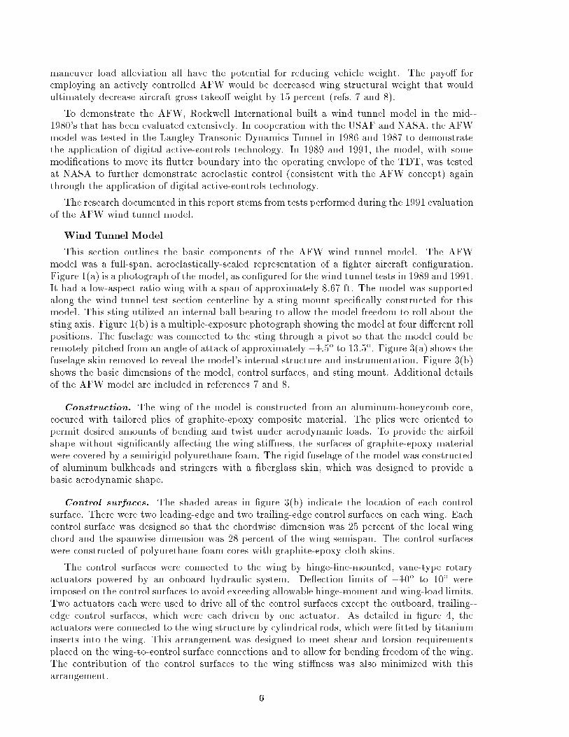
maneuver load alleviation all have the potential for reducing vehicle weight. The payo� foremploying an actively controlled AFW would be decreased wing structural weight that would

ultimately decrease aircraft gross takeo� weight by 15 percent (refs. 7 and 8).

To demonstrate the AFW, Rockwell International built a wind tunnel model in the mid-

1980's that has been evaluated extensively. In cooperation with the USAF and NASA, the AFW

model was tested in the Langley Transonic Dynamics Tunnel in 1986 and 1987 to demonstrate

the application of digital active-controls technology. In 1989 and 1991, the model, with some

modi�cations to move its utter boundary into the operating envelope of the TDT, was tested

at NASA to further demonstrate aeroelastic control (consistent with the AFW concept) again

through the application of digital active-controls technology.

The research documented in this report stems from tests performed during the 1991 evaluation

of the AFW wind tunnel model.

Wind Tunnel Model

This section outlines the basic components of the AFW wind tunnel model. The AFW

model was a full-span, aeroelastically-scaled representation of a �ghter aircraft con�guration.

Figure 1(a) is a photograph of the model, as con�gured for the wind tunnel tests in 1989 and 1991.

It had a low-aspect ratio wing with a span of approximately 8.67 ft. The model was supported

along the wind tunnel test section centerline by a sting mount speci�cally constructed for thismodel. This sting utilized an internal ball bearing to allow the model freedom to roll about the

sting axis. Figure 1(b) is a multiple-exposure photograph showing the model at four di�erent roll

positions. The fuselage was connected to the sting through a pivot so that the model could be

remotely pitched from an angle of attack of approximately �1:5� to 13:5�. Figure 3(a) shows the

fuselage skin removed to reveal the model's internal structure and instrumentation. Figure 3(b)

shows the basic dimensions of the model, control surfaces, and sting mount. Additional details

of the AFW model are included in references 7 and 8.

Construction. The wing of the model is constructed from an aluminum-honeycomb core,

cocured with tailored plies of graphite-epoxy composite material. The plies were oriented to

permit desired amounts of bending and twist under aerodynamic loads. To provide the airfoil

shape without signi�cantly a�ecting the wing sti�ness, the surfaces of graphite-epoxy material

were covered by a semirigid polyurethane foam. The rigid fuselage of the model was constructed

of aluminum bulkheads and stringers with a �berglass skin, which was designed to provide a

basic aerodynamic shape.

Control surfaces. The shaded areas in �gure 3(b) indicate the location of each control

surface. There were two leading-edge and two trailing-edge control surfaces on each wing. Each

control surface was designed so that the chordwise dimension was 25 percent of the local wing

chord and the spanwise dimension was 28 percent of the wing semispan. The control surfaces

were constructed of polyurethane foam cores with graphite-epoxy cloth skins.

The control surfaces were connected to the wing by hinge-line-mounted, vane-type rotary

actuators powered by an onboard hydraulic system. De ection limits of �10� to 10� were

imposed on the control surfaces to avoid exceeding allowable hinge-moment and wing-load limits.

Two actuators each were used to drive all of the control surfaces except the outboard, trailing-

edge control surfaces, which were each driven by one actuator. As detailed in �gure 4, the

actuators were connected to the wing structure by cylindrical rods, which were �tted by titanium

inserts into the wing. This arrangement was designed to meet shear and torsion requirements

placed on the wing-to-control surface connections and to allow for bending freedom of the wing.

The contribution of the control surfaces to the wing sti�ness was also minimized with this

arrangement.

6

Instrumentation. The AFW wind tunnel model was instrumented with several types ofsensors. Strain gauges measured bending and torsion moments and a gyro measured roll rate.

Placement of bending- and torsion-moment strain gauges is shown in �gure 3 and shown in detail

in �gure 5. Primary (1) and secondary (2) strain gauges of each type were positioned at four

stations located inboard and outboard of each wing. Secondary sensor signals were available if

primary sensors failed. The roll-rate gyro was located at an inboard location on the left side of

the model as shown in �gure 3(a). The model was also instrumented with accelerometers and a

roll potentiometer, none of which were used by the RMLA control laws described herein.

Tip ballast stores. Because the model was used to evaluate utter suppression control

laws, the original AFW model was modi�ed before the wind tunnel test in 1989 to move its

utter boundary into the operating envelope of the TDT. This modi�cation consisted of adding

a ballast store to each wing tip, as shown in �gures 1 and 3. A detailed drawing of the tip store

is shown in �gure 6. The store was basically a thin, hollow, aluminum tube with internal ballast

distributed to lower the wing utter boundary to a desired dynamic pressure range. Instead of

a hard attachment, the store was connected to the wing by a pitch-pivot mechanism. The pivot

allowed freedom for the store to pitch relative to the wing surface. When testing for utter, an

internal hydraulic brake held the store to prevent this rotation. This con�guration was called

the coupled tip-ballast-store con�guration. In the event of a utter instability, this brake wasreleased. In the released or decoupled con�guration, the pitch sti�ness of the store was provided

by an internal spring element, shown in �gure 6. The reduced sti�ness of the spring element

(when compared with the hydraulic brake arrangement) signi�cantly increased the frequency of

the �rst torsion mode of the wing. The change in frequency moved the utter condition to higher

dynamic pressures. This behavior was related to the decoupler pylon as discussed in reference 9.

The automatic decoupling of the tip ballasts from the wing structure to rapidly increase the

utter speed of the model during tests in which a utter instability occurred provided a safety

mechanism that prevented damage to the model and the wind tunnel.

Sting mount. The model was supported in the wind tunnel by a sting mount that was

constructed expressly for tests of the AFW model. An internal ball bearing allowed the model

a roll degree of freedom about the sting and an hydraulic braking system inhibited this degree

of freedom. The hydraulic braking system engaged automatically to prevent the umbilical

cables running through the sting mount from snapping during rolling maneuvers exceeding 135�

or �135�.

Digital Controller

The control laws presented in this document were implemented during wind tunnel testsby using a digital controller system (DCS) (ref. 10). The DCS was a real-time, multiple-

function, multi-input/multi-output digital controller developed by NASA as part of the AFW

test program. A schematic in �gure 7 shows how the system was integrated with the AFW

model.

The DCS, as used in the 1991 wind tunnel tests, consisted of a workstation, which housed

three separate special purpose processing units: an integer digital signal processor (DSP), a

oating-point DSP with two microprocessors, and an array processor (AP). A high-speed integer

DSP controlled all the real-time processing including control law execution, data acquisition, and

storage. Actual control law computations were performed with the oating-point DSP. High-

speed direct memory access for the DCS was provided by the AP. In addition, the AP provided

vectorized oating-point processing and served as a backup for the DSP during single-function

control law tests.

7

The DCS was designed to be highly exible in the structure and the dimension of controllaws to be implemented and in the selection of sensors and actuators used. Simultaneous

implementation of control laws was possible. A utter suppression system (FSS) could be tested

in conjunction with the roll-trim system (RTS), the roll rate tracking system (RRTS) or the

RMLA system.

Additional DCS hardware included two analog-to-digital (AD) converters that transformed

up to 64 analog voltage signals from the model instrumentation into digital form and two digital-

to-analog (DA) converters that converted up to 16 controller output signals to analog form.

The interface electronics box shown in �gure 7 �ltered the analog signals being received from

the model or sent to the model by the digital controller. The box contained antialiasing �lters

with either a 25-Hz or 100-Hz break frequency and �rst- or fourth-order roll-o� characteristics.

Notch �lters were also contained in the box and employed by some FSS control laws to provide

additional analog �ltering of either input or output signals. The RMLA control laws did not use

notch �lters, but low pass �lters were included analytically.

Plant Equations

The ARC system was designed to minimize control-surface de ections during rolling maneu-

vers and was experimentally evaluated during the wind tunnel test of the AFW in 1987 (ref. 11).

In that study, the frequency of the commanded input was assumed to be well below the fre-

quency of the �rst exible mode; consequently, the exible modes would not be excited by the

motion of the control surfaces used by the ARC system for roll control. Only rigid-body motion

was used in the design of the ARC system and analytical and experimental results compared

well with the previous study. Consequently, the RMLA control laws presented herein used only

the rigid-body roll equation and load equations in the design model.

Plant Equations of Motion

The rigid-body roll equation of motion for the open-loop wind tunnel model used in both

this study and that of reference 11 is described as follows:

Ixx��� Lp

_�+mgl sin� =

6X

i=1

L�i�i (1)

Many of the coe�cients and variables used in the equation are de�ned in reference 12. However,

equation (1) di�ers in two ways from the equation in reference 12: the control-surface rate

derivatives have been neglected and the quantity mgl sin�, referred to herein as the pendulum

term, has been added. This pendulum term is necessary because the center of gravity of the wind

tunnel model is a distance l below the roll axis of the model. This term is not representative

of a real aircraft and causes equation (1) to be nonlinear. The nonlinear term can be linearized

for small roll angles by the fact that sin� � � (� in radians); however, for the large roll

angles experienced during wind tunnel tests, the small angle assumption is violated. With

this approximation, the pendulum term is 57 percent too large at � = 90�. Nevertheless, this

assumption was still considered reasonable to obtain estimates of behavior with a linearized

model that includes the pendulum e�ect. To simplify the design of control laws, a linearized

model of the plant was desired. To this end, three sets of plant equations were developed. The

�rst set was composed of linearized state-space equations with the nonlinear pendulum term

included explicitly. The second set included a linearized pendulum term in the linearized state-

space equations. The third set was a linearized state-space design model, which contained no

pendulum term. The �rst two sets were simulation models used for evaluation of analytical

results; the last set was used for the actual RMLA control law design. A discussion of the

8

techniques used to identify parameters for the plant equations from experimentally obtaineddata are presented in appendix A. A study of the relative moment contribution of the pendulum

term with respect to the moment due to control-surface de ections was performed to justify the

exclusion of the pendulum term in the design model. The details of this study are presented in

appendix B, but results from the study are presented later in this section.

Nonlinear model. Equation (1) can be expressed in state-space form as

_x = Ax+Bu+Beue (2a)

ue = sin� (2b)

where

x = f _� �gT

u =f �LEOL �TEOL�TEIL

�LEOR�TEOR

�TEIRgT

A =

24

Lp

Ixx0

1 0

35

B =

264L�LEOL

Ixx

L�TEOL

Ixx

L�TEIL

Ixx

L�LEOR

Ixx

L�TEOR

Ixx

L�TEIR

Ixx

0 0 0 0 0 0

375

Be =

24�

mgl

Ixx

0

35

and equation (2b) includes the nonlinear pendulum term explicitly.

An iterative, variable step Kutta-Merson method was used to solve this system analytically.

This integration process is based conceptually on the discretization of the di�erential equations

that represent the model. In this method, an initial value for ue is assumed, and equation (2a) is

then solved for _� and � for the next value of t. The value of � is then used in (2b) to de�ne the

next value of ue. The process is repeated for successive values of t over the time interval desired.

Simulations were performed with this process in the MATRIXx/SystemBuild simulation tool

developed by Integrated Systems, Inc., and described in reference 13.

Linear model. Equations (2a) and (2b) are linearized by assuming sin� � �, which results

in the following linearized model:

_x = Ax+Bu�mgl

Ixx� (3)

By combining the pendulum term with the term Ax of equation (2a), a linearized state-space

representation may then be written as

_x = Alx+Bu (4)

9

where

Al =

24Lp

Ixx�

mgl

Ixx

1 0

35

and x, u, and B are de�ned as for equations (2a) and (2b).

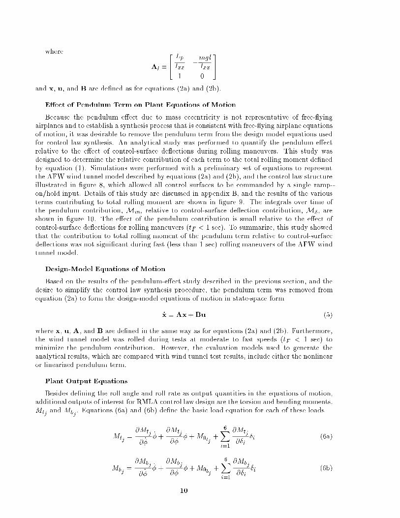
E�ect of Pendulum Term on Plant Equations of Motion

Because the pendulum e�ect due to mass eccentricity is not representative of free- ying

airplanes and to establish a synthesis process that is consistent with free- ying airplane equations

of motion, it was desirable to remove the pendulum term from the design model equations used

for control law synthesis. An analytical study was performed to quantify the pendulum e�ect

relative to the e�ect of control-surface de ections during rolling maneuvers. This study was

designed to determine the relative contribution of each term to the total rolling moment de�ned

by equation (1). Simulations were performed with a preliminary set of equations to represent

the AFW wind tunnel model described by equations (2a) and (2b), and the control law structure

illustrated in �gure 8, which allowed all control surfaces to be commanded by a single ramp-

on/hold input. Details of this study are discussed in appendix B, and the results of the various

terms contributing to total rolling moment are shown in �gure 9. The integrals over time of

the pendulum contribution, Mm, relative to control-surface de ection contribution, M�, are

shown in �gure 10. The e�ect of the pendulum contribution is small relative to the e�ect of

control-surface de ections for rolling maneuvers (tF < 1 sec). To summarize, this study showed

that the contribution to total rolling moment of the pendulum term relative to control-surface

de ections was not signi�cant during fast (less than 1 sec) rolling maneuvers of the AFW wind

tunnel model.

Design-Model Equations of Motion

Based on the results of the pendulum-e�ect study described in the previous section, and the

desire to simplify the control law synthesis procedure, the pendulum term was removed from

equation (2a) to form the design-model equations of motion in state-space form

_x = Ax+Bu (5)

where x, u, A, and B are de�ned in the same way as for equations (2a) and (2b). Furthermore,

the wind tunnel model was rolled during tests at moderate to fast speeds (tF < 1 sec) to

minimize the pendulum contribution. However, the evaluation models used to generate the

analytical results, which are compared with wind tunnel test results, include either the nonlinear

or linearized pendulum term.

Plant Output Equations

Besides de�ning the roll angle and roll rate as output quantities in the equations of motion,

additional outputs of interest for RMLA control law design are the torsion and bending moments,

Mtjand Mbj

. Equations (6a) and (6b) de�ne the basic load equation for each of these loads

Mtj=@Mtj

@ _�

_�+@Mtj

@��+M0tj

+

6X

i=1

@Mtj

@�i�i (6a)

Mbj=@Mbj

@ _�_� +

@Mbj

@��+M0bj

+

6X

i=1

@Mbj

@�i�i (6b)

10

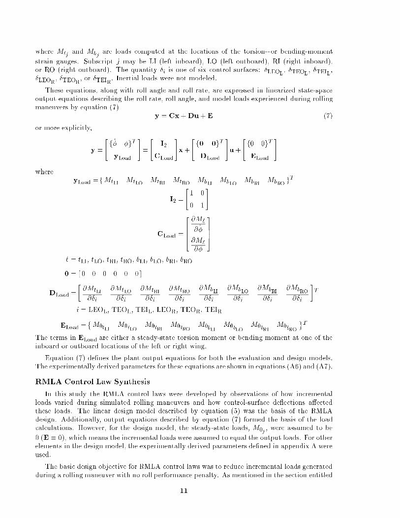
where Mtjand Mbj

are loads computed at the locations of the torsion- or bending-moment

strain gauges. Subscript j may be LI (left inboard), LO (left outboard), RI (right inboard),or RO (right outboard). The quantity �i is one of six control surfaces: �LEOL

, �TEOL, �TEIL,

�LEOR, �TEOR, or �TEIR. Inertial loads were not modeled.

These equations, along with roll angle and roll rate, are expressed in linearized state-space

output equations describing the roll rate, roll angle, and model loads experienced during rolling

maneuvers by equation (7)

y = Cx+Du+ E (7)

or more explicitly,

y =

"f _� �gT

yLoad

#=

"I2

CLoad

#x+

"f0 0gT

DLoad

#u+

"f0 0gT

ELoad

#

whereyLoad =fMtLI

MtLOMtRI

MtROMbLI

MbLOMbRI

MbROgT

I2 =

"1 0

0 1

#

CLoad =

2664@M`

@ _�

@M`

@�

3775

` = tLI; tLO; tRI; tRO; bLI; bLO; bRI; bRO

0 = [ 0 0 0 0 0 0 ]

DLoad=

�@MtLI

@�i

@MtLO

@�i

@MtRI

@�i

@MtRO

@�i

@MbLI

@�i

@MbLO

@�i

@MbRI

@�i

@MbRO

@�i

�T

i = LEOL; TEOL; TEIL; LEOR; TEOR; TEIR

ELoad =�M0tLI

M0tLOM0tRI

M0tROM0bLI

M0bLOM0bRI

M0bRO

T

The terms in ELoad are either a steady-state torsion moment or bending moment at one of the

inboard or outboard locations of the left or right wing.

Equation (7) de�nes the plant output equations for both the evaluation and design models.

The experimentally derived parameters for these equations are shown in equations (A6) and (A7).

RMLA Control Law Synthesis

In this study the RMLA control laws were developed by observations of how incremental

loads varied during simulated rolling maneuvers and how control-surface de ections a�ected

these loads. The linear design model described by equation (5) was the basis of the RMLA

design. Additionally, output equations described by equation (7) formed the basis of the loadcalculations. However, for the design model, the steady-state loads, M0j

, were assumed to be

0 (E = 0), which means the incremental loads were assumed to equal the output loads. For other

elements in the design model, the experimentally derived parameters de�ned in appendix A were

used.

The basic design objective for RMLA control laws was to reduce incremental loads generated

during a rolling maneuver with no roll performance penalty. As mentioned in the section entitled

11

\RMLA Design Concept," this meant developing active RMLA control laws that would attemptto alleviate both bending- and torsion-moment wing loads during fast rolling maneuvers. Somepreliminary studies that used results of control-surface roll and load e�ectiveness from earlier1989 wind tunnel tests showed the trailing-edge inboard pair of control surfaces generatedthe largest rolling moments. However, the outboard control surfaces demonstrated a moresubstantial ability to a�ect incremental loads during rolling maneuvers. These studies impliedthat the outboard surfaces could be de ected a limited amount during a maneuver to alleviateloads, and any roll performance lost because of this actuation of outboard control surfaces couldbe regained by increased de ections of the trailing-edge inboard control surfaces. From initialsimulation studies, it was found that bending- and torsion-moment loads were coupled to eachother and to the angular de ections of the control surfaces. Results of the control surface loade�ectiveness evaluations, described later in this section, verify these initial studies. This couplingof the loads indicated that simplifying the control objective by targeting the reduction of a singletype of load was plausible. Results of another simulation study, summarized in �gure 11, showedthat when the inboard control surfaces were used, torsion-moment peak incremental loads weresigni�cantly larger relative to their steady-state values than the respective bending-momentloads. Based on these preliminary results, the original RMLA objective was modi�ed to targetreductions of only the peak incremental torsion moments rather than those of both the torsionand bending moments. This modi�cation still met the intent of the original research objective.However, by designing control laws to reduce only these key loads, makes the design e�ortsigni�cantly simpler, although care must be taken that the trade-o�s (in this case, increases inthe peak incremental bending moments) are not too severe.

Thus, the RMLA control laws were formulated to use the trailing-edge inboard control surfacepair for maintaining roll performance of the vehicle while outboard control surfaces (leading ortrailing edge) were used to reduce peak incremental torsion-moment loads.

Synthesis Procedure

The RMLA control law synthesis procedure used herein involves four steps, which are outlinedbelow.

1. Evaluate control-surface load e�ectiveness

Evaluate the ability of each control surface to a�ect change in roll and loads during fastrolling maneuvers.

2. Determine potential control law form

Establish e�ective control-surface combinations and a feedback control law form that canpotentially reduce dynamic loads.

3. Determine control law gains

Iterate control system gains for the various control-surface combinations to determine a setof gains that e�ectively reduces dynamic loads during speci�ed rolling maneuvers.

4. Determine control system stability and robustness

Check whether the stability margins are adequate after iterating for a set of control systemgains.

Synthesis Steps

The following section describes the development of the particular RMLA control laws whichare described herein.

12

Evaluate control surface load e�ectiveness. A qualitative procedure was established toevaluate the ability of each outboard control surface to change incremental loads generatedduring a rolling maneuver; in other words, the load e�ectiveness of each outboard control wasevaluated. This method provided su�cient information to determine which direction the leading-edge outboard and trailing-edge outboard control-surface pairs should be de ected during rollingmaneuvers to produce decreases in the incremental loads. For this evaluation, the experimentallydetermined plant equations de�ned in appendix A for dynamic pressure q = 150 psf was used.

Simulations were performed with the same control law structure as the mass eccentricitystudy, which allowed all surfaces to be commanded by a single external ramp-hold input (�g. 8).Right and left control surfaces were de ected di�erentially with a positive de ection of a control-surface pair being de�ned as the left control surface de ected upward (negative) and the rightdownward (positive).

The systematic procedure used to de�ne operation of the outboard control was straight-forward. The procedure was simply to apply speci�ed positive and negative outboard control-surface (di�erential) de ections during simulated rolling maneuvers while the trailing-edgeinboard control surfaces were used to maintain a constant performance.

Five sets of incremental-load time histories were obtained. Figure 12 shows the time historiesof the incremental outboard bending moment obtained for each of these simulations. The �rst setcorresponds to a rolling maneuver performed with the trailing-edge inboard control surfaces only(baseline) to achieve a rolling performance of 90� to 0� in 0.75 sec. The maneuver was performedto determine baseline incremental outboard bending moment. The second set of incremental-load time histories corresponds to a maneuver performed with a 2� di�erential de ection ofthe leading-edge outboard control-surface pair (+LEO) while the trailing-edge inboard control-surface pair was de ected a su�cient amount to maintain the roll performance of 90� to 0� in0.75 sec. The third set of incremental-load time histories was obtained in a similar manner exceptthat the leading-edge outboard control surface was de ected �2� (�LEO) during the maneuver.The fourth and �fth sets of incremental-load time histories were obtained by performing thesame rolling maneuvers with the leading-edge outboard control-surface de ections held at 0�

and the trailing-edge outboard control-surface de ections speci�ed to be 2� and �2� during twoseparate rolling maneuvers, (+TEO and �TEO, respectively). The dashed line indicates thetime at which the simulated rolling maneuvers passed 0�.

By plotting the �ve sets of incremental loads, it can be seen how outboard control-surfacede ections a�ect the incremental outboard bending moment. As can be seen in �gure 12,negative de ections of both outboard control-surface pairs were found to cause decreases inoutboard incremental bending loads. Similar results were obtained for the inboard incrementalbending loads and inboard incremental torsion loads; however, decreases in outboard incrementaltorsion loads resulted only from negative de ections of the outboard trailing-edge controlsurfaces. A summary of the qualitative results of this study is shown in table 1. Increaseor decrease indicates whether the peak incremental loads increased or decreased when comparedwith the peak incremental loads of the baseline maneuver. Control-surface di�erential de ectionis also indicated. Based on these results, the most e�ective control surfaces for reducing allincremental loads would most likely be the outboard trailing-edge control-surface pair.

Determine potential control law form. Since the rolling maneuvers were de�ned in termsof time to roll, it was determined that the command to roll would be proportional to rollrate. It was also observed during the simulations that the incremental loads tended to be(linearly) proportional to the roll rate. Thus, direct feedback of the roll rate to control surfacescould reasonably be used to counteract the incremental loads, as well as to roll the model.The trailing-edge inboard control surfaces were chosen to maintain roll performance while the

13

outboard control surfaces were used to reduce incremental loads. In summary, the RMLA controllaws described herein were designed to (1) actuate the trailing-edge inboard control surfaces inthe positive direction di�erentially (left upward, right downward) to e�ect roll, (2) actuatethe leading-edge outboard and/or trailing-edge outboard control-surface pairs in the negativedirection di�erentially (left downward, right upward) to reduce loads, and (3) adjust all thecontrol-surface de ections based on the roll rate.

Based on the above reasons, the RMLA control law structure illustrated in �gure 13 wasselected as the basic RMLA control law form to be used. The structure includes roll-rate feedbackto the trailing-edge inboard, leading-edge outboard, and trailing-edge outboard control-surfacepairs. Left and right wing control surfaces in each pair are de ected di�erentially. In addition tothe roll-rate feedback, the roll-rate command describing the desired roll-rate performance is alsosent to the trailing-edge inboard control-surface pair. Outboard control surfaces are commandedonly by roll-rate feedback.

Since the �rst exible mode frequency was above 7 Hz, a 8.75-Hz low-pass �lter de�ned by

T�i =4:65(105)

s3+ 206:71s2+ 14804s+ 4:65(105)(8)

was included in each loop of the system to minimize the e�ect of the RMLA control laws on the exible modes that would be present during tests and to smooth the input command.

The RMLA control laws can be expressed in linearized state-space form as

_xc = Fcxc+Gfzf +Gcom_�com

u = [DcHc]xc+ Efzf + Ecom_�com

9=; (9)

where

Ecom= [Kcom 0 0 0 ]T

Ef = [ 0 KTEI KTEO KLEO ]T

and xc represents the controller states, zf the feedback control input _�, and _�com the commandedroll rate.

Determine control law gains. Initial gains were chosen from the information determinedduring the control-surface e�ectiveness study and the RMLA control law structure de�ned in�gure 13. The most important aspect of the RMLA control law design was that the control lawsproduce outboard control-surface de ections during a rollingmaneuver to counteract incrementalloads. In addition, it was necessary that the control laws produce reasonable control-surfacede ections and rates that did not saturate the actuators at dynamic pressure ranges of 150 to250 psf. A target rolling maneuver performance criterion of 90� to 0� in 0.75 sec was selectedfor the RMLA design. The input gain Kcom and feedback gains KTEI, KTEO, and KLEO werethen iterated until the model met its target performance while reducing analytically predictedpeak incremental loads and meeting robustness design objectives analytically.

Three control laws, referred to herein as A, B, and baseline, were developed with exper-imentally derived equations of motion and equations of plant output. Each control law wasdesigned to meet test objectives at a design q = 150 psf and a corresponding Mach numberof 0.33. The control laws were then also evaluated for the design model at q = 250 psf and

14

Mach number of 0.44. Control law A was de�ned by roll-rate feedback to the trailing-edge in-board control-surface pair and from the trailing-edge outboard control-surface pair (K

LEO= 0).

Control law B was de�ned by roll-rate feedback to the trailing-edge inboard control-surface pairand to the leading-edge outboard control-surface pair (K

TEO= 0). Finally, the baseline control

law was de�ned by roll-rate feedback from the trailing-edge inboard control-surface pair only(K

TEO= 0 and K

LEO= 0). A summary of control system gains is listed in table 2.

Determine control system stability and robustness. System stability was determinedanalytically for each closed-loop system at the two design conditions, q = 150 and 250 psf,with each of the three control laws de�ned previously. The system stability was determined byperforming an eigenvalue analysis on the linearized state-space model of the closed-loop systemfor each control law. For these analyses, the plant was de�ned by equations (10), where _� is theonly output used for the RMLA feedback control law

_x = Ax+Bu

zf = Cfx

)(10)

where x, u, A, and B are de�ned by equation (5) and

zf = _�

Cf = [1 0 ]

For the stability analyses discussed herein, the experimentally de�ned models described inappendix A were used for the equations, and the roll-rate command _�com was assumed to be 0.

Each of the three control laws presented were stable. Table 3 shows the eigenvalues of theclosed-loop system for each of the RMLA control laws at q = 150 psf that correspond to themodel parameters de�ned in equation (A6) and those values for q = 250 psf that correspond tomodel parameters de�ned in equation (A7). Note that all eigenvalues have negative real partswith zero imaginary parts and therefore lie in the left complex plane, which implies a stableclosed-loop system. The eigenvalues for the baseline system are not shown.

Once system stability is established, stability margins can be determined with the methoddescribed in reference 14. The stability margins for each of the designed RMLA control laws waspredicted in terms of simultaneous gain and phase changes in each of the loops of a multiloopsystem. The universal gain and phase margin diagram shown in �gure 14, which is based on�gure 2 in reference 14, provides a mechanism for predicting regions of guaranteed stability inan operating frequency range. Reference 14 shows that the stability of the perturbed system isguaranteed provided the minimum singular value of the linear system return di�erence matrixis greater than � = L

�1� I.

To determine the stability margins in a multiloop system, the system return-di�erence matrixat the plant input must be determined and the minimum singular values calculated. This matrixis de�ned by [I+GH(i!)], where

G = �[DcHc(Is� Fc)�1Gf +Ef ] (11)

is the controller transfer matrix and

H = [Cf(Is�A)�1B] (12)

is the plant transfer matrix. The closer the minimum singular value is to 0 at any frequency,the less robust the system is to modeling errors. The stability margins were determined for

15

the q = 150 psf design model. For this model, the closed-loop system with the baseline control

law implemented was determined analytically to have a minimum singular value of 0.49. The

closed-loop systems, with control laws A and B implemented, were determined to have singular

values of 0.79 and 0.77, respectively. In �gure 14, a horizontal line drawn at �min

= 0:79

and intersecting the 20� phase line at �4:2 dB and 12.8 dB indicates that control law A has a

guaranteed minimum gain margin of �4:2 dB and 12.8 dB with at least a 20� phase perturbation

margin in all loops. This process illustrates the use of the diagram to determine gain and phase

margins for control law A. The RMLA control law B and the baseline control law have guaranteed

minimum gain margins of �4 dB and 11 dB and �2 dB and 5 dB, respectively, with 20� phase

perturbation margin in all loops. For other phase margin perturbations, di�erent gain margins

could be achieved.

Wind Tunnel, Test Procedures, and Data Reduction for RMLA Performance

Evaluation

Wind Tunnel

The Langley Transonic Dynamics Tunnel (TDT) is a closed-circuit, continuous ow wind

tunnel with a 16-ft-square test section with cropped corners. It operates at stagnation pressures

from near vacuum to slightly above atmospheric pressure and at Mach numbers to 1.2. Tunnel

Mach number may be varied simultaneously or independently with dynamic pressure. Either air

or a heavy gas can be used as the test medium. During the current investigation, air was used

as the test medium. The TDT is equipped with hydraulic bypass valves, which may be opened

rapidly to reduce test section dynamic pressure and Mach number when utter is encountered.

A more detailed description of the TDT is presented in reference 15.

Test Procedures

Initially, control laws A and B and the baseline control law were tested at tunnel test

conditions of q = 150, 200, and 250 psf and Mach numbers of 0.33, 0.39, and 0.44, respectively.

The model was con�gured for each of these tests so that open-loop utter would not be incurred.

Each rolling maneuver controlled by RMLA commenced with the model positioned at a roll angle

of 90� and was terminated shortly after the model rolled through 0�. Maneuvers at q = 150

and 200 psf were performed with the tip ballast coupled; however, those at q = 250 psf were

performed with the tip ballast decoupled to raise the open-loop utter dynamic pressure above

the test dynamic pressure. Figure 15 shows the operating envelope in air for the TDT. The test

points at which single-function RMLA control laws (no utter suppression control law active)

were tested with the tip ballasts coupled are indicated by solid circles, and the test point with

the tip ballasts decoupled is indicated by a solid square. The open-loop utter point is also

identi�ed. Table 4 summarizes the conditions for single-function RMLA control law tests.

Rolling maneuvers were also performed above the open-loop utter dynamic pressure at

q = 250 and 260 psf with the tip ballast coupled. These test points are identi�ed with open

circles in �gure 15. For these maneuvers, RMLA control law B was implemented simultaneously

with an active utter suppression system (FSS) by using the control law described in reference 16.

During these multiple-function maneuvers, the rolling maneuvers commenced with the model

positioned at 70� roll angle instead of 90� and were terminated as the model rolled through �20�

because at 90� the measured dynamic loads were too close to the preselected load limits of the

trip system for the wind tunnel model. This adjustment of the rolling maneuver starting point

and termination point allowed less interruptions of the test because the multifunction rolling-

maneuver tests could be conducted in a dynamic load range where the trip system was less likely

to trigger the tunnel bypass system. Table 5 summarizes conditions for this multiple-function

RMLA + FSS test.

16

Figure 16 is a description of how the RMLA controllers were commanded during tests andhow the roll-rate commands were implemented on the digital controller. The model was �rstrolled to and held at its initial roll position with the RTS. When ready for a rolling maneuver,control of the model was switched to the RMLA control system within the digital controller,and control of the model by the RTS was discontinued. At this point, control-surface commandswere determined by a speci�ed RMLA control law (control law A or B, or the baseline controllaw). As shown in �gure 16, the roll rate was commanded by a ramp-on/hold input duringthe maneuver. Di�erent roll rates could be speci�ed to achieve desired time-to-roll performancerequirements. A ramp-o� roll-rate command was used to terminate the maneuver after themodel passed through the termination roll angle. When the model roll rate was below 5 deg/sec(denoted _�cap in the �gure), digital control of the model was switched from RMLA back to RTSonce again. To simplify the control law design process, the rolling-maneuver load control lawswere only designed to reduce loads for the portion of the maneuver prior to the point where theroll-rate commands were ramped o�. This point is referred to as the time to roll, identi�ed astF in �gure 16. The comparison of the results described herein are for the design region from 0to tF.

For both the single-function RMLA tests and the multiple-function tests, rolling maneuverswere repeated at each test point for several di�erent roll-rate commands de�ned by a scale factortimes a nominal command input to assure that data obtained were in the performance range ofinterest. These scale factors ranged from 0.8 to 1.4 and are listed in �gure 17.

Data Reduction for RMLA Performance Evaluation

Before describing the results obtained from wind tunnel tests, a brief discussion of thedata reduction method used to evaluate the RMLA performance is necessary. First, peakincremental loads had to be extracted from test data for each rolling maneuver performed.Four incremental loads were examined: outboard incremental bending moment �MbO

, inboardincremental bending moment �MbI

, outboard incremental torsion moment �MtO, and inboard

incremental torsion moment �MtI. These incremental loads were de�ned to be one-half the

right wing incremental load (with respect to the initial steady-state load value) minus one-halfthe corresponding left wing incremental load, respectively for each load as described by

�Mbj(t) =

1

2

��MbRj

(t)�MssbRj

��

�MbLj

(t)�MssbLj

��

�Mtj(t) =

1

2

nhMtRj

(t)�MsstRj

i�

hMtLj

(t)�MsstLj

io

9>>>=>>>;

(13)

where j = O or I and the terms with ss as a subscript represent the corresponding steady-statevalues. The steady-state loads at the start of each rolling maneuver are summarized in table 6for each dynamic pressure. Table 7 shows corresponding static load limits for each type of loadto provide a reference level for each load.

Peak incremental loads equal to the maximum absolute value of the incremental loads thatoccurred during each rolling maneuver were computed by

�Mbj= max

t

����Mbj(t)���

�Mtj= max

t

����Mtj(t)���

9>=>; (14)

where j = O or I.

17

Results and Discussion

In this section, incremental-load time histories obtained during RMLA-controlled rollingmaneuvers are compared to baseline loads, and the reduction in peak incremental loads arepresented. The resulting load alleviation achieved with RMLA control law A and control law Bare presented and the performance of the two control laws are also compared. Finally, anevaluation of the multiple-function performance of RMLA control law B implemented with a utter suppression control law is presented.

Experimental Results

Results were calculated with equations (13) and (14) for all RMLA-controlled rollingmaneuvers and the baseline rolling maneuvers. The resulting incremental loads and peakincremental loads for all maneuvers and test conditions are too numerous to discuss and comparein this paper; however, typical results are shown and comparisons are made in the subsectionentitled \Time History Comparisons of Incremental Loads." Discussion of incremental-loadreductions and summaries of results are presented in subsections entitled \Typical LoadAlleviation Results" and \Overall Analysis of Experimental Results," respectively.

Time history comparisons of incremental loads. Some typical time history resultsobtained during wind tunnel evaluation for RMLA control laws A and B are shown in �gures 18and 19, respectively. In both of these �gures, the incremental loads obtained during a rollingmaneuver controlled by the speci�ed RMLA control law and a corresponding baseline maneuverhaving nearly the same performance time to roll 90� are compared. Since the performance timesare nearly the same, a comparison can be made between the actual RMLA and the baseline loadtime histories, rather than comparing only the RMLA-controlled peak incremental loads withinterpolated peak values from baseline rolling maneuvers. The rolling maneuver was a 90� to0� roll at q = 200 psf with a performance time tF of 0.66 sec for control law A, 0.645 sec forcontrol law B, and 0.65 sec for the baseline control law. Roll-rate and roll-angle time historiesare shown in parts (a) and (b), respectively, of �gures 18 and 19. The vertical dashed lineindicates the approximate point in time at which the RMLA-controlled rolling maneuver wasconsidered terminated, and the roll-rate command ramped o�. Since the following discussioncan generally be applied to the results shown for both controllers, only results of control law Bcorresponding to �gure 19 will be discussed in further detail, but the results of control law A(�g. 18) are presented for completeness.

Decreases in incremental torsion moments are shown in �gures 19(c) and 19(d) for most ofthe rolling maneuver from 90� to 0�. There is a substantial decrease in peak incremental torsionmoments. The outboard and inboard torsion moments of 495.1 and 1565 in-lb, respectively, at0.49 sec for the baseline control law decrease to 265.6 and 885.8 in-lb, respectively, at 0.4 sec forcontrol law B. This substantial reduction in peak incremental torsion moments is typical of allthe RMLA-controlled rolling maneuvers.

Similar comparisons for the incremental bending moments, �gures 19(e) and 19(f), indicateincreases in the peak incremental load for the outboard and inboard bending moments, but allthe peak incremental loads are more nearly the same for the RMLA-controlled maneuver. Oneincremental load that is approximately three times larger than all the others for the baselinemaneuver, namely the inboard torsion moment, is brought within the same level of load as allthe others. Since the design criteria did not include the peak incremental bending moments, itis not surprising to see an increase in these as a result of lowering the peak incremental torsionmoments.

Figure 18 shows similar decreases and increases in incremental loads for control law A;however, the signi�cance of the load increases to the severity of trade-o� between decreases

18

and increases in incremental loads is still to be determined. The next two sections address thisissue in more detail.

Typical load alleviation results. Table 8 summarizes the percent changes in peak

incremental loads shown in �gures 18 and 19 for both control laws A and B, and bar graphs of

these changes are shown in �gure 20. Figure 20(a) summarizes the changes for control law A

in peak incremental loads relative to the baseline. The �gure shows that the peak outboard

incremental torsion moment is reduced by 27.4 percent relative to the baseline case and peak

inboard incremental torsion moment is reduced by 52.3 percent. There is a 14.7 percent increase

in the peak value of inboard incremental bending moment. Peak outboard incremental bending

moment for control law A, however, is shown to increase by approximately 2.5 times with respect

to the baseline.

Figure 20(b) illustrates similar results from the tests of RMLA control law B. As before,

reductions in incremental torsion moments were achieved. Peak outboard incremental torsion

moment was reduced by 46.4 percent and peak inboard incremental torsion moment was reduced

by 43.4 percent. Increases, however, are seen in both outboard and inboard incremental bending-

moment peak values of 39.7 percent and 16.0 percent, respectively.

To gauge the signi�cance of these results for each load, a comparison can be made between

changes in peak incremental loads and the static load limits, which are listed in table 7. For

instance, the increase over the baseline of 16.0 percent in peak inboard incremental bending

moment shown in �gure 20(b) is less than 0.3 percent of the minimum inboard bending-moment

static load limit. Similarly, the percentage increase in peak outboard incremental bending

moment represents less than 2.1 percent of the minimum outboard bending-moment static load

limit. On the contrary, the percentage decreases in peak outboard and inboard incremental

torsion moments represent larger percentages (16.1 percent and 7.6 percent) of their respective

minimum torsion-moment load limits.

Table 9 summarizes the percent changes in incremental loads relative to minimum static load

limits for both control laws. In both of these cases, the changes in the outboard torsion moment

are signi�cant since the amount of load alleviation because of implementation of the RMLA

control law represents a substantial portion of the capacity of each wing to support outboard

torsion moments. The small percentage increases in the bending moments because of control

law B are considered to be an inconsequential trade-o� for the signi�cant percentage decreases intorsion moments relative to the minimum static load limits. Note that the 12.8 percent increase

in peak incremental outboard bending moment relative to the minimum static load limits for

control law A might indicate a signi�cant trade-o� penalty for the decreases in torsion-moment

peak incremental loads, warranting further investigation.

Overall analysis of experimental results. This section provides an analysis of the results

of all the rolling maneuvers performed in the TDT with the two RMLA control laws described

herein and the baseline control law. The same trends indicated in the previous comparisons

occurred between all the RMLA-controlled maneuvers and the baseline maneuvers. The peak

incremental loads were calculated from the experimental data with equations (14) for all the

rolling maneuvers performed and these results are presented in table 10. The RMLA-controlled

rolling maneuvers had di�erent performance times from the baseline maneuvers. Test time did

not permit performing additional maneuvers to obtain the same performance times. Because

it was necessary to compare the RMLA maneuvers with baseline maneuvers with the same

performance times, peak incremental loads obtained for baseline maneuvers were interpolated

as a function of performance time to correspond to performance times equal to those achieved

during RMLA-controlled maneuvers. These calculations are presented in table 11, and the

interpolated values were used for all the results discussed subsequently.

19

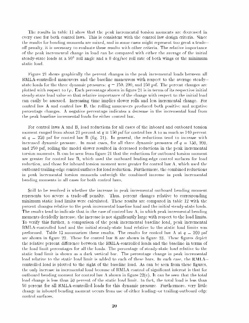
The results in table 11 show that the peak incremental torsion moments are decreased inevery case for both control laws. This is consistent with the control law design criteria. Since

the results for bending moments are mixed, and in some cases might represent too great a trade-

o� penalty, it is necessary to evaluate these results with other criteria. The relative importance

of the peak incremental change in load can be compared with either the average of the initial

steady-state loads at a 90� roll angle and a 0 deg/sec roll rate of both wings or the minimum

static load.

Figure 21 shows graphically the percent changes in the peak incremental loads between all

RMLA-controlled maneuvers and the baseline maneuvers with respect to the average steady-

state loads for the three dynamic pressures: q = 150, 200, and 250 psf. The percent changes are

plotted with respect to tF. Each percentage shown in �gure 21 is in terms of its respective initial

steady-state load value so that relative importance of the change with respect to the initial load

can easily be assessed. Increasing time implies slower rolls and less incremental change. For

control law A and control law B, the rolling maneuvers produced both positive and negative

percentage changes. A negative percentage indicates a decrease in the incremental load from

the peak baseline incremental loads for either control law.

For control laws A and B, load reductions for all cases of the inboard and outboard torsion

moment ranged from about 21 percent at q = 150 psf for control law A to as much as 140 percent

at q = 250 psf for control law B (�g. 21). In general, the reductions tend to increase with

increased dynamic pressure. In most cases, for all three dynamic pressures of q = 150, 200,

and 250 psf, rolling the model slower resulted in decreased reductions in the peak incremental

torsion moments. It can be seen from �gure 21 that the reductions for outboard torsion moment

are greater for control law B, which used the outboard leading-edge control surfaces for load

reduction, and those for inboard torsion moment were greater for control law A, which used the

outboard trailing-edge control surfaces for load reduction. Furthermore, the combined reductions

in peak incremental torsion moments outweigh the combined increase in peak incremental

bending moments in all cases for both control laws.

Still to be resolved is whether the increase in peak incremental outboard bending moment

represents too severe a trade-o� penalty. Thus, percent changes relative to corresponding

minimum static load limits were calculated. These results are compared in table 12 with the

percent changes relative to the peak incremental baseline load and the initial steady-state loads.

The results tend to indicate that in the case of control law A, in which peak incremental bending

moments decidedly increase, the increase is not signi�cantly large with respect to the load limits.

To verify this further, a comparison of the peak incremental baseline load, peak incremental

RMLA-controlled load and the initial steady-state load relative to the static load limits was

performed. Table 13 summarizes these results. The results for control law A at q = 200 psf

are shown in �gure 22. Those for control law B are shown in �gure 23. These �gures depict

the relative percent di�erence between the RMLA-controlled loads and the baseline in terms of

the load limit percentages for all the loads. The percentage of steady-state load relative to the

static load limit is shown as a dark vertical bar. The percentage change in peak incremental

load relative to the static load limit is added to each of these bars. In each case, the RMLA-

controlled load is plotted to the right of the baseline load. As can be seen from these �gures,

the only increase in incremental load because of RMLA control of signi�cant interest is that for

outboard bending moment for control law A shown in �gure 22(c). It can be seen that the total

load change is less than 50 percent of the static load limit. In fact, the total load is less than

50 percent for all RMLA-controlled loads for this dynamic pressure. Furthermore, very little

change in inboard bending moment occurs from use of either leading- or trailing-outboard edge

control surfaces.

20

Summary of experimental results. In general, control law B, which used the leading-edgeoutboard control-surface pair, resulted in greater reductions in outboard incremental torsion

moments than control law A. The reverse is true for the inboard incremental torsion moments.

This suggests that, for the AFW wind tunnel model, the leading-edge outboard control-surface

pair is more e�ective at reducing the outboard incremental torsion moments than the trailing-

edge outboard control-surface pair. Likewise, the trailing-edge outboard control-surface pair is

more e�ective in decreasing inboard incremental torsion moments. In both cases, the targeted

design goal, namely, reducing peak incremental torsion moments, was substantially met.

Control law A and control law B di�ered more signi�cantly in how peak incremental bending

moments were a�ected during rolling maneuvers. It can be observed from table 12 that peak

values of incremental bending moments increased 285 percent relative to a baseline maneuver

for maneuvers controlled by control law A and less than 42 percent increases for comparable

maneuvers controlled by control law B; however, these increases proved to be only 56.6 percent

increase with respect to the initial loads, and only 17.6 percent with respect to the minimum

static load limit. Furthermore, it was demonstrated that in all cases, the RMLA-controlled load

plus the corresponding initial steady-state load does not exceed 57 percent of the static load

limit.

In general, control law B demonstrated the better overall RMLA characteristics relative to

the limit loads. (Compare �g. 23 with �g. 22.) The percent changes for bending-moment

loads with respect to the steady-state loads were shown to be small. These results con�rm

initial perceptions that only torsion moment need to be targeted for load reduction in designing

an RMLA control law, as stated in the RMLA Design Concept section. With control law B,

substantially large reductions were achieved in both inboard and outboard incremental torsion

moments without signi�cant increases in incremental bending moments. A signi�cantly higher

reduction was achieved in outboard torsion moment with control law B than for either the

inboard or outboard torsion moments for control law A. Since the reductions relative to static

load limits are most signi�cant for outboard torsion moments, control law B is considered to be

the more e�ective of the two for rolling-maneuver load alleviation.

Comparison of Experimental and Analytical Results

To evaluate how well the analytical models could be used to predict load reduction during

controlled rolling maneuvers, simulated maneuvers were performed on the computer at dynamic

pressures of q = 150 and 250 psf and at performance times of 0.65 and 0.75 sec with the non-

linear equations of motion (2a) and (2b) and the output equation (7). Experimentally derived

parameters de�ned by equations (A6) and (A7) were used in the equations. Figure 24 shows

the percent changes between simulated and experimental peak incremental torsion moments ob-

tained during RMLA-controlled maneuvers relative to those obtained during baseline-controlled

maneuvers with the same performance times. Dashed lines indicate analytical results and the

solid lines show the experimental results. Figures 24(a) and 24(c) show results for control law A,

and 24(b) and 24(d) for control law B.

As can be seen from �gure 24, the analytical model, in general, predicts the trends in reduction

for the incremental torsion moments; however, the analytical model is conservative in predicting

the absolute value of reduction in all cases.

Multiple-Function Control Law Performance Results

Successful rolling maneuvers 6 percent and 11 percent above the open-loop utter dynamic

pressure were achieved in tests with RMLA control law B and a utter suppression control law

implemented simultaneously on the digital controller (ref. 16). Flutter did not occur during the

maneuvers, which implies that the utter suppression control law was suppressing the instability

21

during roll. It was not possible to quantify incremental load reduction since time did not allowbaseline data at the same dynamic pressures with the AFW model in the tip-ballast-coupled

con�guration to be obtained. Thus, a qualitative evaluation of load reduction could not be

made above open-loop utter. However, based on comparisons of incremental loads with the

FSS control law operating at subcritical dynamic pressures for which comparable baseline data

were available, namely q = 150 and 200 psf, it is likely that incremental load reduction occurred.

Since rolling maneuvers had to be ramped o� quickly to avoid exceeding the roll angle of the

model on the sting, load trip limits were incurred during the ramp-o� portion of the rolling

maneuvers in some cases. However, trip limits based upon static load limits were incurred only

when the roll command was ramped o�. Since the RMLA control laws were not designed to

reduce loads during the ramp-o� portion of the roll command, and trip limits were not incurred

during the ramp-on/hold portion of the rolling maneuvers, it can be stated that control law B

did not induce excessive incremental loads during rolling maneuvers above the open-loop utter

dynamic pressure.

By observing control surface de ection time histories during a rolling maneuver, it was seen

that the RMLA and utter suppression control laws operated simultaneously without signi�cant

interference. Figure 25 shows control surface de ections during a roll which occurred in 0.63 sec

at q = 250 psf with simultaneous operation of RMLA and FSS. The time histories are for right

wing control surfaces only. The dashed lines indicate the point in time at which the roll was

terminated. The leading-edge outboard and the trailing-edge inboard control-surface de ections

due to RMLA are shown in �gures 25(a) and 25(b). Trailing-edge outboard control-surface

de ection is due to the utter suppression control law and is shown in �gure 25(c). Figure 25(c)

shows that the trailing-edge outboard control surface was oscillating at about 9.5 Hz. This

frequency of oscillation was due to the FSS control law for utter suppression, during and after

the rolling maneuvers.

Thus, it was demonstrated that the RMLA and utter suppression control laws can be

implemented simultaneously on the AFW digital controller and operate e�ectively together

during rolling maneuvers at dynamic pressures 11 percent above the critical utter dynamic

pressure.

Concluding Remarks

This report provides a systematic synthesis methodology to design RMLA feedback control

laws. Two relatively simple RMLA control laws, referred to herein as A and B, were designed and

implemented on a digital control computer. Control law A used trailing-edge surfaces and control

law B used leading-edge surfaces to alleviate loads. These control laws were experimentally

evaluated and shown to e�ectively and reliably reduce incremental torsion loads on the AFW

wind tunnel model in the Transonic Dynamics Tunnel (TDT). In addition, it was demonstrated

through wind tunnel tests that a digital control computer can be used with great versatility

to perform a multifunction task such as suppressing utter and reducing loads during rolling

maneuvers. The analytical model provided conservative estimates of peak incremental load

reduction.

Load alleviation during controlled rolling maneuvers of a model in the wind tunnel was

demonstrated. Leading-edge and trailing-edge control surfaces were actively employed by digital

control to accomplish this objective.

Torsion moment reduction was targeted as the design objective, and experimental evaluation

of two RMLA controllers showed up to a 61.6 percent reduction in peak incremental torsion

moments when compared with those generated by corresponding baseline rolling maneuvers

at equivalent dynamic pressures with the same time-to-roll performance. Incremental bending

moments were evaluated. Results varied, but in general showed relatively small load changes

22

when compared with static load limits during the same rollingmaneuver. The maximum increase

was a peak incremental outboard bending moment of 17.6 percent relative to the static load limit

for control law A; however, the resulting combined steady-state and peak incremental load of

less than 60 percent of the static load limit was within load limit margins.

Control law B showed at least 14 percent greater reduction capability of the outboard torsion

moment and at least a 31 percent reduction in inboard incremental torsion moment relative to

a baseline rolling maneuver than control law A. This was achieved with less than a 2 percent

increase in peak incremental bending moments relative to static load limits. This comparison

demonstrates that the use of outboard leading-edge control surfaces may be more e�ective for

reducing outboard torsion loads during rolling maneuvers than outboard trailing-edge controls

while still signi�cantly reducing inboard torsion loads with relatively little penalty from increases

in incremental bending moments. These results con�rm initial perceptions that only torsion

moment need to be targeted for load reduction in designing an RMLA control law for this

model.

It was demonstrated by experiment that the RMLA and utter suppression control laws

could be implemented simultaneously and operate e�ectively together during rolling maneuvers

at dynamic pressures 11 percent above the open-loop utter dynamic pressure.

NASALangley Research Center

Hampton, VA 23681-0001

August 8, 1994

23

Appendix A

Aeroelastic Analysis and Parameter Identi�cation

Equations of motion were developed during tests to have a state-space representation of AFWloads suitable for RMLA control law design and evaluation. System equations were de�ned byeither equations (2), (4), or (5), depending upon how the pendulum term was included. Theoutput equations were de�ned by equation (7). Equations were developed to model the plantat both q = 150 and 250 psf with experimental data to de�ne the parameters in the linearizedequations. For q = 250 psf, which is above the open-loop utter dynamic pressure for thetip-ballast-coupled con�guration, the experimental data were acquired only for the decoupledcon�guration. Time did not allow data for the coupled con�guration to be obtained. Sincedecoupled data were the best that could be obtained for the higher dynamic pressure testcondition prior to RMLA control law design, decoupled equations were used only to performevaluations, not control law design. To be consistent with control law design for free- yingaircraft, and in light of the results of the study on the e�ect of mass eccentricity, the center ofmass was assumed to be on the roll axis (l = 0) for the RMLA control law design. Since thisassumption implies the pendulum term is 0, only the remaining linearized equations were usedfor the design models. Evaluation models included either the nonlinear or linear pendulum term.Test procedures used to acquire the necessary experimental data to identify the parameters inthe linearized equations are identi�ed below.

Data Acquisition

In order to identify the moment and load coe�cients due to roll and roll rate, experimentaldata were acquired from rolling maneuvers in which control-surface de ections were 0, that is, byperforming free-fall maneuvers of the AFW model at q = 150 and 250 psf. More speci�cally, ateach dynamic pressure, the model was positioned at a roll angle of 90� with the roll-trim system(RTS). The model was then released (control surfaces were set to 0) and the model was allowedto return to its equilibrium position at or near a roll angle of 0� without control-surface actuationduring the maneuver. The restoring force acting on the model was due solely to eccentricity ofthe model-mass c.g. below the roll axis.

Additional experimental load data were obtained during tests to determine the rolling andmoment coe�cients due to control-surface de ection by holding the model at a roll angle of 0�

with the sting-mounted braking system, and then de ecting each control surface, �i, one at atime, at the rate of 5 deg/sec from 0 to 10�.

Damping-Coe�cient Parameter Identi�cation

With data obtained during the free-fall maneuvers, values for the parameters in the state-space equations were estimated in the following manner.

To determine the damping-in-roll element of A, namely,

Lp

Ixx

equation (2) was used. Since all the �i = 0 in free fall, and the pendulum term was de�nedfor the model, the only undetermined value for these simulations was the damping-in-roll term.Consequently, analytical simulations of free fall were performed with this model in which thedamping-in-roll coe�cient was varied until the peak roll rate matched that observed in the testdata. Figure 26(a) shows the actual free-fall experimental data at q = 150 psf with the �nalsimulated curve superimposed.

24

Load Parameter Identi�cation

Total loads during rolling maneuvers are de�ned by

yLoad = CLoadx+DLoadu+ ELoad (A1)

where

yLoad =nMtLI

; MtLO; MtRI

; MtRO; MbLI

; MbLO; MbRI

; MbRO

oT

CLoad = [C1 : C2]

C1 =

�@M`

@ _�

�

C2 =

�@M`

@�

�

` = tLI; tLO; tRI; tRO; bLI; bLO; bRI; bRO

Since there was no control-surface actuation during the free-fall maneuver, the load equationsduring these maneuvers are completely de�ned by the matrices CLoad and ELoad and can bedetermined from free-fall data. To identify elements of these matrices, it was �rst assumedthat each load, M , acting on the model during roll could be described by the following linearequation,

M =@M

@ _�_�+

@M

@��+M0 (A2)

Inertial loads were not modeled.

Next the elements of ELoad, de�ned by the elements, M0, were evaluated by averaging thetotal loads for short intervals of time after the model reached its equilibrium position when _�and � are both 0.

The elements of C2 in the partitioned matrix CLoad were determined by estimating thecoe�cient of � in equation (A2) for each load M . This term results from the fact that avariation in steady-state loads existed in the data between the model at 90� and 0� roll angles.Since steady-state load values for roll-angle positions between 90� and 0� were not available,a straight line approximation was made so that the experimental models matched steady-statewind tunnel loads at 90� and 0� roll angles, and the partial of M with respect to � was de�nedas the constant slope,

@M

@�=

M90��M0�

90�(A3)

The coe�cient of _� in equation (A2) de�ning the element of C1 corresponding to load M inthe partitioned matrix CLoad, was rewritten in terms of known quantities as follows:

@M

@ _�=

�M �

@M@�

��M0

�_�

(A4)

Each term in equation (A4) is a function of time; hence, division by the roll rate implies divisionby time-correlated values of the numerator and denominator. Because the acceleration is zeroat the peak roll rate, it was assumed that the unmodeled inertial load would also be zero at thispoint because of its proportional relationship with acceleration. Thus, to obtain C1, the average

25

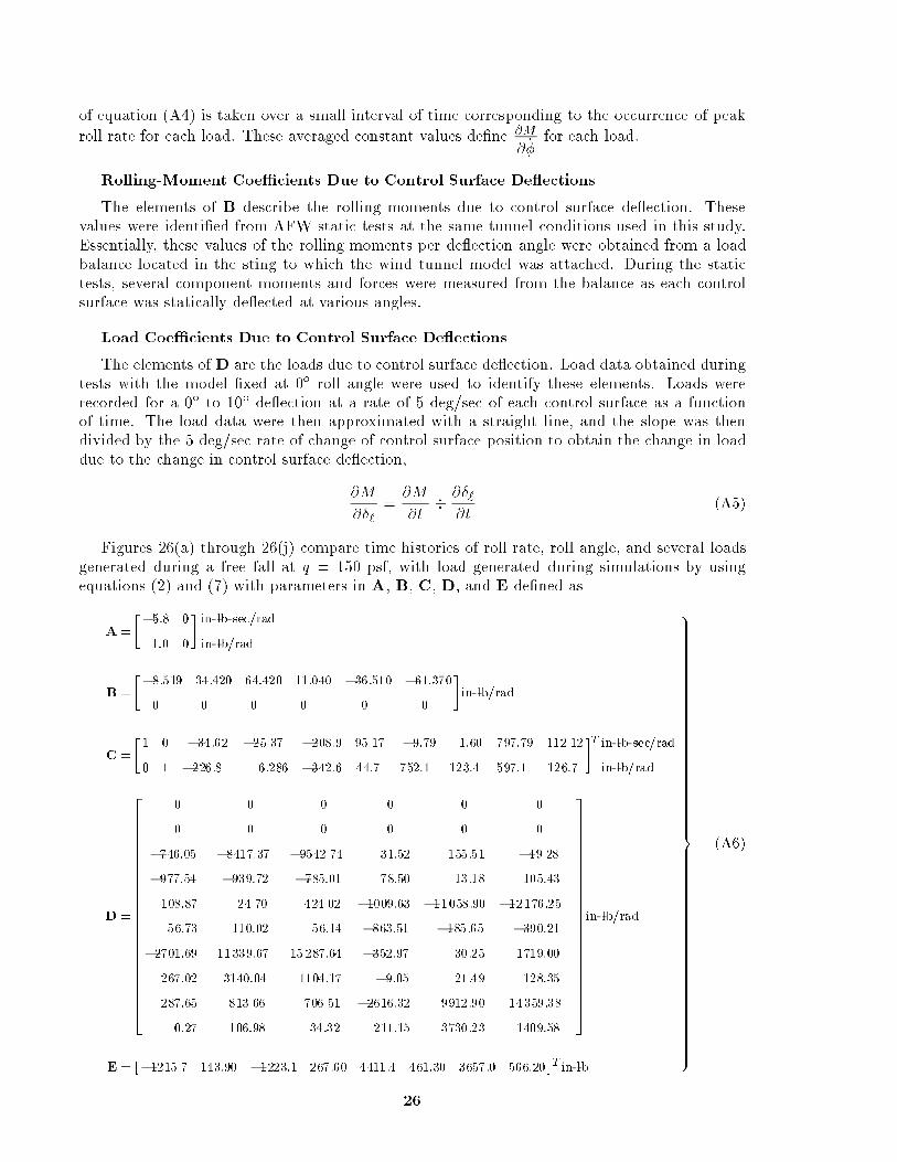
of equation (A4) is taken over a small interval of time corresponding to the occurrence of peak

roll rate for each load. These averaged constant values de�ne @M

@ _�for each load.

Rolling-Moment Coe�cients Due to Control Surface De ections

The elements of B describe the rolling moments due to control surface de ection. Thesevalues were identi�ed from AFW static tests at the same tunnel conditions used in this study.Essentially, these values of the rolling moments per de ection angle were obtained from a loadbalance located in the sting to which the wind tunnel model was attached. During the statictests, several component moments and forces were measured from the balance as each controlsurface was statically de ected at various angles.

Load Coe�cients Due to Control Surface De ections

The elements of D are the loads due to control surface de ection. Load data obtained duringtests with the model �xed at 0� roll angle were used to identify these elements. Loads wererecorded for a 0� to 10� de ection at a rate of 5 deg/sec of each control surface as a functionof time. The load data were then approximated with a straight line, and the slope was thendivided by the 5 deg/sec rate of change of control surface position to obtain the change in loaddue to the change in control surface de ection,

@M

@�`=

@M

@t�@�`

@t(A5)

Figures 26(a) through 26(j) compare time histories of roll rate, roll angle, and several loadsgenerated during a free fall at q = 150 psf, with load generated during simulations by usingequations (2) and (7) with parameters in A, B, C, D, and E de�ned as

A=

��5:8 0

1:0 0

�in-lb-sec=rad

in-lb=rad

B=

��8:519 34:420 64:420 11:040 �36:510 �61:370

0 0 0 0 0 0

�in-lb=rad

C=

�1 0 �34:62 �25:37 �208:9 95:17 �9:79 1:60 797:79 112:12

0 1 �226:8 6:286 �342:6 44:7 752:1 123:4 597:1 126:7

�Tin-lb-sec=rad

in-lb=rad

D=

26666666666666666666664

0 0 0 0 0 0

0 0 0 0 0 0

�746:05 �8417:37 �9542:74 31:52 155:51 �49:28

�977:54 �939:72 �785:01 78:50 13:18 105:43

108:87 24:70 424:02 �1009:63 �11058:90 �12176:25

56:73 110:02 56:14 �863:51 �185:65 �390:21

�2701:69 11339:67 15287:64 �352:97 30:25 1719:00

267:02 3140:04 1104:17 �9:05 21:49 128:35

287:65 813:66 706:51 �2616:32 9912:90 14359:38

0:27 106:98 34:32 211:15 3730:23 1409:58

37777777777777777777775

in-lb=rad

E= [�1215:7 143:90 �1223:1 267:60 4411:4 461:30 3657:0 566:20]Tin-lb

9>>>>>>>>>>>>>>>>>>>>>>>>>>>>>>>>>>>>>>>>>>>>>>=>>>>>>>>>>>>>>>>>>>>>>>>>>>>>>>>>>>>>>>>>>>>>>;

(A6)

26

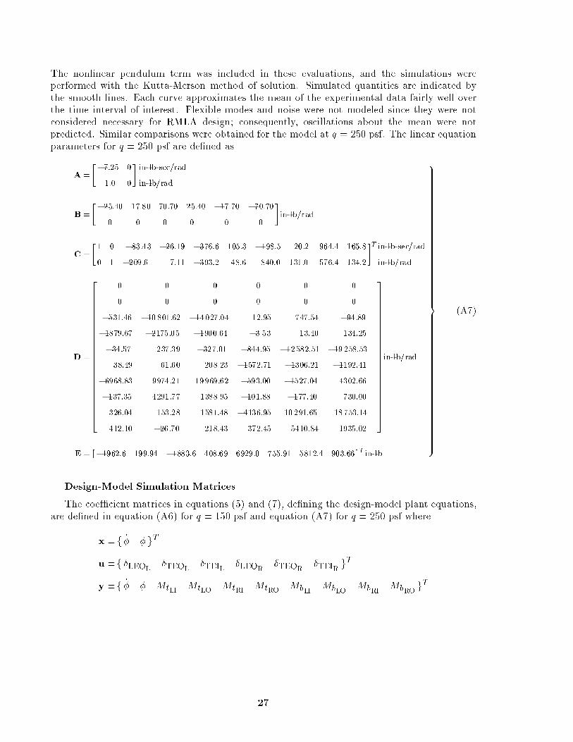
The nonlinear pendulum term was included in these evaluations, and the simulations wereperformed with the Kutta-Merson method of solution. Simulated quantities are indicated bythe smooth lines. Each curve approximates the mean of the experimental data fairly well overthe time interval of interest. Flexible modes and noise were not modeled since they were notconsidered necessary for RMLA design; consequently, oscillations about the mean were notpredicted. Similar comparisons were obtained for the model at q = 250 psf. The linear equationparameters for q = 250 psf are de�ned as

A=

��7:25 0

1:0 0

�in-lb-sec=rad

in-lb=rad

B=

��25:40 17:80 70:70 25:40 �17:70 �70:70

0 0 0 0 0 0

�in-lb=rad

C=

�1 0 �83:43 �26:19 �376:6 105:3 �198:5 20:2 964:4 165:8

0 1 �209:6 7:11 �393:2 48:6 840:0 131:0 576:4 134:2

�Tin-lb-sec=rad

in-lb=rad

D=

26666666666666666666664

0 0 0 0 0 0

0 0 0 0 0 0

�531:46 �10801:62 �14027:04 12:95 747:54 �94:89

�1879:67 �2175:05 �1900:64 �3:53 13:40 134:25

�34:57 237:39 �327:01 �844:95 �12582:51 �19258:53

38:49 61:60 208:23 �1572:71 �1306:21 �1192:41

�6968:83 9974:21 19969:62 �593:00 �1527:04 4302:66

�137:35 4291:77 1388:95 �101:88 �177:40 730:00

326:04 153:28 1581:48 �4136:95 10291:65 18753:14

412:10 �26:70 218:43 372:45 5410:84 1935:02

37777777777777777777775

in-lb=rad

E= [�1962:6 199:94 �1883:6 408:69 6929:0 755:91 5812:4 903:66]Tin-lb

9>>>>>>>>>>>>>>>>>>>>>>>>>>>>>>>>>>>>>>>>>>>>>>=>>>>>>>>>>>>>>>>>>>>>>>>>>>>>>>>>>>>>>>>>>>>>>;

(A7)

Design-Model Simulation Matrices

The coe�cient matrices in equations (5) and (7), de�ning the design-model plant equations,are de�ned in equation (A6) for q = 150 psf and equation (A7) for q = 250 psf where

x =f _� �gT

u =f �LEOL �TEOL�TEIL

�LEOR�TEOR

�TEIRgT

y =f _� � MtLI MtLO MtRI MtRO MbLIMbLO

MbRIMbROgT

27

Appendix B

Calculation of Mass Eccentricity E�ects

Separating equation (1) into four moment contribution terms, the relative importance of each

rolling moment contribution can be assessed. The four moment contributions are inertial rolling

moment induced roll acceleration

Mxx = Ixx�� (B1)

the aerodynamic rolling moment induced by roll rate

Mp = Lp _� (B2)

the pendulum rolling moment due to mass eccentricity

Mm= mgl sin� (B3)

and the aerodynamic rolling moment due to control surface de ections

M� =

6X

i=1

L�i�i (B4)

Initially, simulations used a preliminary set of equations to represent the AFW wind tunnel

model described by equations (2a) and (2b) were performed with a control law structure that

allowed all surfaces to be commanded by a single external ramp-hold input �c (i.e., each �i = �c).

The control structure is illustrated in �gure 8. Right and left control surfaces were de ected

di�erentially. For individual control surfaces, it was assumed that downward de ection was

positive. The convention for pairs of control surfaces used in the RMLA development and

design was that a positive (di�erential) de ection caused the left control surface to be de ected

upward and the right downward (positive). Di�erent �c commands resulted in various time-to-

roll-90� performance times tF ranging in value from 0.5 sec to 3 sec. The parameters used in the

equations of motion for this mass eccentricity study are de�ned in table B1. The roll angle �(t)

was determined from the simulation by using the variable step Kutta-Merson method, and each

of the terms de�ned by equations (B1) through (B4) were plotted. Figure 9 shows the results of

two of these simulations at q = 150 psf for two di�erent performance times. Figures 9(a) and (9c)

show the time histories of the roll angle and roll rate, � and _�, in terms of degrees and deg/sec,

respectively. Figures 9(b) and (9d) show Mxx, Mp, Mm, and M� for each tF , respectively. The

performance time to roll from 90� to 0� for �gures 9(a) and (9b) is tF = 0:58 sec, as indicated

in �gure 9(a). For �gures 9(c) and (9d), tF = 1:8 sec, as indicated in �gure 9(c). By comparingthe magnitudes of Mm, and M� for 0 < t < tF , for each tF , it can be seen that jMmj is small

relative to jM�j during the faster rolling maneuver (tF = 0:58 sec) once the control surfaces

are de ected. However, jMmj is signi�cantly larger relative to jM�j during the slower rolling

maneuver (tF = 1:8 sec). In fact, jMmj is larger than jM�j during the �rst 1.2 sec.

To better quantify the total pendulum e�ect, integrals of the magnitudes of the pendulum

rolling moment and the aerodynamic rolling moment were generated as functions of the time

required to roll from 90� to 0�.

Mm=

t=tFZ

t=0

jMmjdt =

t=tFZ

t=0

jmgl sin�(t)jdt (B5)

28

and

M� =

t=tFZ

t=0

jM�jdt =

t=tFZ

t=0

�����6Xi=1

L�i�i

�����dt (B6)

Figure 10 shows the results of these integral calculations over a range of performance times from

0.5 to 3 sec for the same model described above at q = 150 psf in which the �i were control surface

commands that achieved the speci�ed times to roll. The points corresponding to tF = 0:58 sec

and tF = 1:8 sec are identi�ed on the plot. It can be seen that Mm is small relative to M�

during fast rolling maneuvers (tF < 1 sec); however, Mm is large relative to M� during slow

rolling maneuvers (tF > 1 sec), which provides a signi�cant restoring force that aids the rolling

maneuver.

This same trend in relative sizes of Mm and M� could be seen in simulations at other

dynamic pressures and other combinations of control surface de ections, including closed-loop

simulations. Rolling faster reduces the contribution of the pendulum rolling moment to the total

rolling moment relative to the aerodynamic rolling moment due to control surface de ections.

Table B1. Mass Eccentricity SimulationModel

mgl, lb-in . . . . . . . . . . . . . . . . . . . . . . 1329.5

Ixx, lb-in-sec2

. . . . . . . . . . . . . . . . . . . . . 256.9

Lp, lb-in-sec . . . . . . . . . . . . . . . . . . . . . 1184.4

L�LEO;L, lb-in/deg . . . . . . . . . . . . . . . . . . . �2188

L�TEO;L, lb-in/deg . . . . . . . . . . . . . . . . . . . . 8841

L�TEI;L, lb-in/deg . . . . . . . . . . . . . . . . . . . . 16501

L�LEO;R, lb-in/deg . . . . . . . . . . . . . . . . . . . . 2836

L�TEO;R, lb-in/deg . . . . . . . . . . . . . . . . . . . �9378

L�TEI;R, lb-in/deg . . . . . . . . . . . . . . . . . . . �15764

M�, lb-in-sec, at|

tF= 0.58 sec . . . . . . . . . . . . . . . . . . . . . 2.34

tF= 0.96 sec . . . . . . . . . . . . . . . . . . . . . 1.54

tF= 1.80 sec . . . . . . . . . . . . . . . . . . . . . 0.724

Mm, lb-in-sec, at|

tF= 0.58 sec . . . . . . . . . . . . . . . . . . . . . 0.567

tF= 0.96 sec . . . . . . . . . . . . . . . . . . . . . 0.884

tF= 1.80 sec . . . . . . . . . . . . . . . . . . . . . 1.425

29

References

1. O'Connell, R. F.: Design, Development and Implementation of an Active Control System for Load Alleviation

for a Commercial TransportAirplane. AGARD-R-683, Feb. 1980. (Available fromDTIC asADA082 959.)

2. Rollwagen, G.; Ellgoth, H.; and Beuck, G.: Identi�cation of Dynamic Response, Simulation and Design of a

Highly Nonlinear Digital Load Alleviation System for a Modern Transport Aircraft. ICAS Proceedings|1990,

Sept. 1990, pp. 427{433. (Available as ICAS-90-1.3.4.)

3. Sandford, Maynard C.; Abel, Irving; and Gray, David L.: Development and Demonstration of a Flutter-

Suppression System Using Active Controls. NASA TRR-450, 1975.

4. Noll, T. E.; and Huttsell, L. J.: Wing Store Active Flutter Suppression|Correlation of Analyses and Wind-

Tunnel Data. J. Aircr., vol. 16, no. 7, July 1979, pp. 491{497.

5. Roger, KennethL.; Hodges, Garold E.; and Felt, Larry: Active Flutter Suppression|AFlight TestDemonstra-

tion. J. Aircr., vol. 12, no. 6, June 1975, pp. 551{556.

6. Sensburg, O.; Honlinger, H.; Noll, T. E.; and Huttsell, L. J.: Active Flutter Suppression on an F-4F Aircraft.

J. Aircr., vol. 19, no. 5, May 1982, pp. 354{359.

7. Miller, Gerald D.: Active Flexible Wing (AFW) Technology. AFWAL-TR-87-3096, U.S. Air Force, Feb. 1988.

(Available fromDTIC as ADB131 204.)

8. Perry, Boyd, III; Cole, Stanley R.; and Miller, Gerald D.: A Summary of the Active Flexible Wing Program.

A Collection of Technical Papers|AIAA Dynamics Specialist Conference, Apr. 1992, pp. 1{10. (Available as

AIAA-92-2080-CP and NASATM-107655.)

9. Reed, WilmerH., III; Foughner, JeromeT., Jr.; andRunyan, HarryL., Jr.: Decoupler Pylon: ASimple, E�ective

Wing/Store Flutter Suppressor. J. Aircr., vol. 17, no. 3,Mar. 1980, pp. 206{211.

10. Hoadley, S. T.; and McGraw, S. M.: The Multi-Input/Multi-Output Multi-Function Digital Controller System

for the AFWWind-Tunnel Model. A Collection of Technical Papers|AIAA Dynamics Specialists Conference,

Apr. 1992, pp. 30{38. (Available as AIAA-92-2083 and NASATM-107600.)

11. Perry, Boyd, III; Dunn, H. J.; and Sandford, Maynard C.: Control Law Parameterization for an Aeroelastic

Wind-Tunnel Model Equipped With an Active Roll Control System and Comparison With Experiment. A

Collection of Technical Papers, Part 1|AIAA/ASME/ASCE/AHS 29th Structure, Structural Dynamics and

Materials Conference, Apr. 1988, pp. 41{56. (Available as AIAA-88-2211.)

12. Etkin, Bernard: Dynamics of Flight. John Wiley & Sons, Inc., 1959.

13. MATRIXx/SystemBuild User's Guide. Version 2.04X, Integrated Systems, Inc., 1990.

14. Mukhopadhyay, V.; and Newsom, J. R.: A Multi-loop System Stability Margin Study Using Matrix Singular

Values. J. Guid., Control, & Dyn., vol. 7, no. 5, Sept.{Oct. 1984, pp. 582{587.

15. Yates, E. Carson, Jr.; Land, Norman S.; and Foughner, Jerome T., Jr.: Measured and Calculated Subsonic and

Transonic Flutter Characteristics of a 45� Sweptback Wing Planform in Air and in Freon-12 in the Langley

Transonic Dynamics Tunnel. NASA TND-1616, 1963.

16. Mukhopadhyay, Vivek: Flutter Suppression Digital Control LawDesign and Testing for the AFWWind-Tunnel

Model. A Collection of Technical Papers|AIAA Dynamics Specialist Conference, Apr. 1992, pp. 156{161.

(Available as AIAA-92-2095-CP.)

30

Table 1. Load E�ectiveness Trends

�TEI, deg �TEO, deg �LEO, deg MbOMbI

MtOMtI

6.4 2 Increase Increase Increase Increase

8.7 �2 Decrease Decrease Decrease Decrease

7.9 2 Increase Increase Increase

7.3 �2 Decrease Decrease Increase Decrease

Table 2. Control Law Gains at q = 150 psf

Gains Control law A Control law B Baseline

Kcom 0.3500 0.3000 0.3500

KTEI �.0625 �.0667 �.0500KTEO �.0384 0 0

KLEO 0 .0356 0

Table 3. Eigenvalues of Closed-Loop Systems

q = 150 psf q = 250 psf

Control law Real Imaginary Real Imaginary

�0.327 0 �0.176 0A �1.606 0 �2.954 0

�0.358 0 �0.286 0B �1.453 0 �1.820 0

Table 4. Test Conditions for Single-Function Open-Loop

Tests With Control Laws A and B

q, psf Mach Tip ballast Flutter suppression

150 0.33 Coupled O�200 .38 Coupled O�250 .44 Decoupled O�

31

Table 5. Test Conditions for Multiple-Function Tests

With Control Law B

q, psf Mach Tip ballast Flutter suppression

250 0.44 Coupled On

260 .45 Coupled On

Table 6. Steady-State Loads at Start of Rolling Maneuvers (90�)

Dynamic

pressure, psf Wing TMO, in-lb TMI, in-lb BMO, in-lb BMI, in-lb

150 Left 69.6 �1932.9 800.8 6207.3

Right 377.3 �1261.1 789.9 4555.3

Average magnitude 223.4 1597.0 795.4 5381.3

200 Left 54.5 �2378.7 964.2 7394.6

Right 415.0 �1585.1 948.7 5434.0

Average magnitude 234.8 1981.9 956.5 6414.3

250 Left 40.4 �2712.3 1052.2 8401.5

Right 469.7 �2016.0 1155.1 6322.4

Average magnitude 255.1 2364.2 1103.7 7362.0

Table 7. Static Load Limits

Load limits for|

Wing TMO, in-lb TMI, in-lb BMO, in-lb BMI, in-lb

Left 1627.0 8929.0 4099.0 20 965.0

Right 1425.0 9434.0 3546.0 18 084.0

Minimum 1425.0 8929.0 3546.0 18 084.0

Table 8. Percent Change in Peak Incremental Loads Relative to Baseline Load Limits

for Control Laws Having Nearly the Same Performance Time at q = 200 psf

Time to roll Peak incremental loads for|

90�, sec TMO, in-lb TMI, in-lb BMO, in-lb BMI, in-lb

Baseline 0.65 495.1 1565.0 185.7 352.2

RMLA A 0.66 359.6 747.1 638.0 403.8

Percent change from baseline �27.4 �52.3 243.6 14.7

RMLA B 0.645 265.6 885.8 259.5 408.6

Percent change from baseline �46.4 �43.4 39.7 16.0

32

Table 9. Percent Change in Peak Incremental Loads Relative to Minimum Static Load

Limits for Control Laws Having Nearly the Same Performance Time at q = 200 psf

Time to roll Peak incremental loads for|

90�, sec TMO, in-lb TMI, in-lb BMO, in-lb BMI, in-lb

Baseline 0.65 495.1 1565.0 185.7 352.2

RMLA A 0.66 359.6 747.1 638.0 403.8

Percent change relative to limit �9.5 �9.2 12.8 0.3

RMLA B 0.645 265.6 885.8 259.5 408.6

Percent change relative to limit �16.1 �7.6 2.1 0.3

Table 10. Peak Incremental Loads From Experimental Data for Baseline

Dynamic Control Time to roll Peak incremental loads for|

pressure, psf law 90�, sec TMO, in-lb TMI, in-lb BMO, in-lb BMI, in-lb

150 Baseline 0.670 391.6 1206.0 180.9 313.6

150 Baseline .705 343.7 1102.0 164.9 342.2

150 Baseline .825 304.3 988.9 118.1 413.0

200 Baseline 0.575 580.0 1829.0 282.1 423.3

200 Baseline .650 495.1 1565.0 185.7 352.2

200 Baseline .805 394.1 1256.0 130.8 459.9

250 Baseline 0.555 719.1 2239.0 312.5 414.7

250 Baseline .645 636.2 1803.0 269.0 363.1

250 Baseline .665 544.4 1617.0 244.8 460.4

250 Baseline .795 506.7 1497.0 168.4 429.1

150 A 0.675 308.4 679.5 493.8 313.3

150 A .695 300.7 699.5 488.4 361.8

150 A .805 263.4 523.2 415.4 279.2

200 A 0.635 376.3 628.5 731.1 442.7

200 A .660 359.6 747.1 638.0 403.8

200 A .770 302.1 570.6 551.3 341.2

250 A 0.600 405.0 776.0 915.4 560.0

250 A .640 394.4 741.1 825.2 590.6

250 A .735 335.2 615.9 696.8 486.6

150 B 0.650 251.1 858.1 250.8 334.6

150 B .675 225.6 787.2 234.4 307.6

150 B .780 178.0 684.7 164.8 455.7

200 B 0.615 279.0 1064.0 294.3 450.1

200 B .645 265.6 885.8 259.5 408.6

200 B .740 205.1 772.9 217.7 547.3

250 B 0.630 293.4 909.1 328.0 366.2

250 B .740 218.0 821.1 230.1 498.4

250 B .770 226.4 700.4 240.5 531.0

33

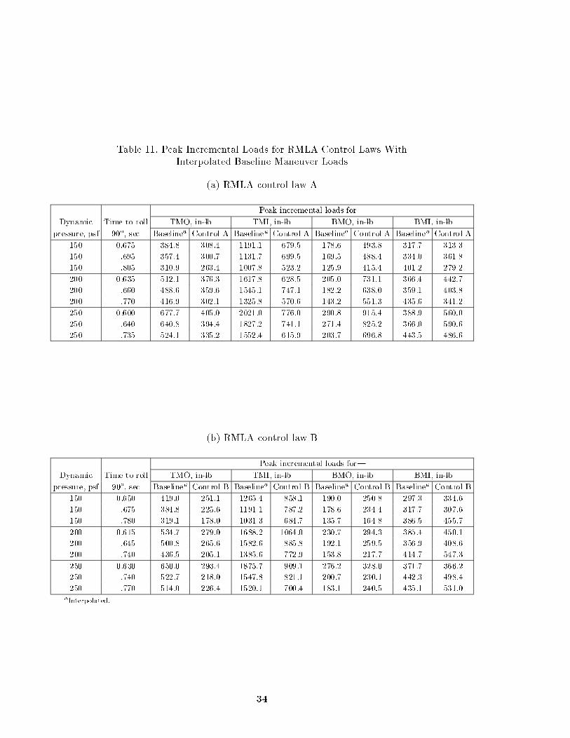
Table 11. Peak Incremental Loads for RMLA Control Laws WithInterpolated Baseline Maneuver Loads

(a) RMLA control law A

Peak incremental loads for|

Dynamic Time to roll TMO, in-lb TMI, in-lb BMO, in-lb BMI, in-lb

pressure, psf 90�, sec Baselinea Control A Baselinea Control A Baselinea Control A Baselinea Control A

150 0.675 384.8 308.4 1191.1 679.5 178.6 493.8 317.7 313.3

150 .695 357.4 300.7 1131.7 699.5 169.5 488.4 334.0 361.8

150 .805 310.9 263.4 1007.8 523.2 125.9 415.4 401.2 279.2

200 0.635 512.1 376.3 1617.8 628.5 205.0 731.1 366.4 442.7

200 .660 488.6 359.6 1545.1 747.1 182.2 638.0 359.1 403.8

200 .770 416.9 302.1 1325.8 570.6 143.2 551.3 435.6 341.2

250 0.600 677.7 405.0 2021.0 776.0 290.8 915.4 388.9 560.0

250 .640 640.8 394.4 1827.2 741.1 271.4 825.2 366.0 590.6

250 .735 524.1 335.2 1552.4 615.9 203.7 696.8 443.5 486.6

(b) RMLA control law B

Peak incremental loads for|

Dynamic Time to roll TMO, in-lb TMI, in-lb BMO, in-lb BMI, in-lb

pressure, psf 90�, sec Baselinea Control B Baselinea Control B Baselinea Control B Baselinea Control B

150 0.650 419.0 251.1 1265.4 858.1 190.0 250.8 297.3 334.6

150 .675 384.8 225.6 1191.1 787.2 178.6 234.4 317.7 307.6

150 .780 319.1 178.0 1031.3 684.7 135.7 164.8 386.5 455.7

200 0.615 534.7 279.0 1688.2 1064.0 230.7 294.3 385.4 450.1

200 .645 500.8 265.6 1582.6 885.8 192.1 259.5 356.9 408.6

200 .740 436.5 205.1 1385.6 772.9 153.8 217.7 414.7 547.3

250 0.630 650.0 293.4 1875.7 909.1 276.2 328.0 371.7 366.2

250 .740 522.7 218.0 1547.8 821.1 200.7 230.1 442.3 498.4

250 .770 514.0 226.4 1520.1 700.4 183.1 240.5 435.1 531.0

aInterpolated.

34

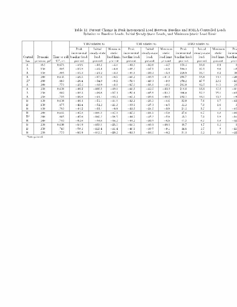
Table 12. Percent Change in Peak Incremental Load Between Baseline and RMLA-Controlled Loads

Relative to Baseline Loads, Initial Steady-State Loads, and Minimum Static Load Limit

TMO relative to| TMI relative to| BMO relative to|

Peak Initial Miminum Peak Initial Miminum Peak Initial Miminum Peak

incremental steady-state static incremental steady-state static incremental steady-state static increme

Control Dynamic Time to roll baseline load, load, load limit, baseline load, load, load limit, baseline load, load, load limit, baseline

law pressure, psf 90�, sec percent percent percent percent percent percent percent percent percent perce

A 150 0.675 �19.8 �34.2 �5.4 �43.0 �32.0 �5.7 176.5 39.6 8.9 1

A 150 .695 �15.9 �25.4 �4.0 �38.2 �27.1 �4.8 188.2 40.1 9.0 �8

A 150 .805 �15.3 �21.2 �3.3 �48.1 �30.3 �5.4 229.9 36.4 8.2 30

A 200 0.635 �26.5 �57.8 �9.5 �61.2 �49.9 �11.1 256.7 55.0 14.8 �20

Aa 200 .660 �26.4 �54.9 �9.1 �51.6 �40.3 �8.9 250.2 47.7 12.9 �12

A 200 .770 �27.5 �48.9 �8.1 �57.0 �38.1 �8.5 285.0 42.7 11.5 21

A 250 0.600 �40.2 �106.9 �19.1 �61.6 �52.7 �13.9 214.8 56.6 17.6 �44

A 250 .640 �38.5 �96.6 �17.3 �59.4 �45.9 �12.2 204.0 50.2 15.6 �61

A 250 .735 �36.0 �74.1 �13.3 �60.3 �39.6 �10.5 242.1 44.7 13.9 �9

B 150 0.650 �40.1 �75.1 �11.8 �32.2 �25.5 �4.6 32.0 7.6 1.7 �12

B 150 .675 �41.4 �71.2 �11.2 �33.9 �25.3 �4.5 31.2 7.0 1.6 3

B 150 .780 �44.2 �63.1 �9.9 �33.6 �21.7 �3.9 21.5 3.7 .8 �17

B 200 0.615 �47.8 �108.9 �17.9 �37.0 �31.5 �7.0 27.6 6.7 1.8 �16

Ba 200 .645 �47.0 �100.2 �16.5 �44.0 �35.2 �7.8 35.1 7.0 1.9 �14

B 200 .740 �53.0 �98.6 �16.2 �44.2 �30.9 �6.9 41.5 6.7 1.8 �32

B 250 0.630 �54.9 �139.8 �25.0 �51.5 �40.9 �10.8 18.7 4.7 1.5 1

B 250 .740 �58.3 �119.4 �21.4 �46.9 �30.7 �8.1 14.6 2.7 .8 �12

B 250 .770 �55.9 �112.7 �20.2 �53.9 �34.7 �9.2 31.4 5.2 1.6 �22aInterpolated.

Table 13. Percent Loads Relative to Minimum Static Load Limits for

RMLA-Controlled, Baseline, and Initial Steady-State Loads

Load, percent, for|

TMO TMI BMO

Control Dynamic Time to roll

law pressure, psf 90�, sec Baseline RMLA Initial Baseline RMLA Initial Baseline RMLA Initial Bas

A 150 0.675 27.0 21.6 15.7 13.3 7.6 17.9 5.0 13.9 22.4 1

A 150 .695 25.1 21.1 15.7 12.7 7.8 17.9 4.8 13.8 22.4 1

A 150 .805 21.8 18.5 15.7 11.3 5.9 17.9 3.6 11.7 22.4 2

A 200 0.635 35.9 26.4 16.5 18.1 7.0 22.2 5.8 20.6 27.0 2

A 200 .660 34.3 25.2 16.5 17.3 8.4 22.2 5.1 18.0 27.0 2

A 200 .770 29.3 21.2 16.5 14.8 6.4 22.2 4.0 15.5 27.0 2

A 250 0.600 47.6 28.4 17.9 22.6 8.7 26.5 8.2 25.8 31.1 2

A 250 .640 45.0 27.7 17.9 20.5 8.3 26.5 7.7 23.3 31.1 2

A 250 .735 36.8 23.5 17.9 17.4 6.9 26.5 5.7 19.7 31.1 2

B 150 0.650 29.4 17.6 15.7 14.2 9.6 17.9 5.4 7.1 22.4 1

B 150 .675 27.0 15.8 15.7 13.3 8.8 17.9 5.0 6.6 22.4 1

B 150 .780 22.4 12.5 15.7 11.6 7.7 17.9 3.8 4.6 22.4 2

B 200 0.615 37.5 19.6 16.5 18.9 11.9 22.2 6.5 8.3 27.0 2

B 200 .645 35.1 18.6 16.5 17.7 9.9 22.2 5.4 7.3 27.0 2

B 200 .740 30.6 14.4 16.5 15.5 8.7 22.2 4.3 6.1 27.0 2

B 250 0.630 45.6 20.6 17.9 21.0 10.2 26.5 7.8 9.2 31.1 2

B 250 .740 36.7 15.3 17.9 17.3 9.2 26.5 5.7 6.5 31.1 2

B 250 .770 36.1 15.9 17.9 17.0 7.8 26.5 5.2 6.8 31.1 2

Tip-ballast-store and

flutter stopper mechanism

L-89-12442

(a) AFW model mounted in the Langley TDT prior to tests.

L-89-12446

(b) Multiple-exposure photograph showing the model at four di�erent roll positions.

Figure 1. Photographs of the AFW model modi�ed for the 1989 and 1991 wind tunnel tests and mounted inthe Langley Transonic Dynamics Tunnel.

37

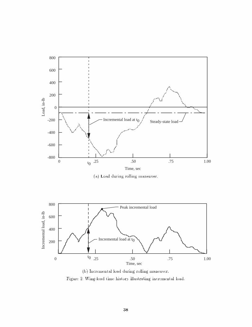
Time, sec

Loa

d, in

-lb

AAAAAAAAAAAAAAAAAAAAAAAAAAAAAAAAAAAAAAAAA

AAAAAAA

AAAAAAAAAAAAAAAAAAAAAAAAAAAAAAAAAAAAAAAAAAAAAAAAAAAAAAAAAAAAAAAAAAAAAA

-200

-800

-600

-400

0

200

400

600

800

1.00.50.25 .750 t0

Incremental load at t0 Steady-state load

(a) Load during rolling maneuver.

Incr

emen

tal l

oad,

in-l

b

0

200

400

600

800

Time, sec1.00.50.25 .75t0

Peak incremental load

Incremental load at t0

(b) Incremental load during rolling maneuver.

Figure 2. Wing-load time history illustrating incremental load.

38

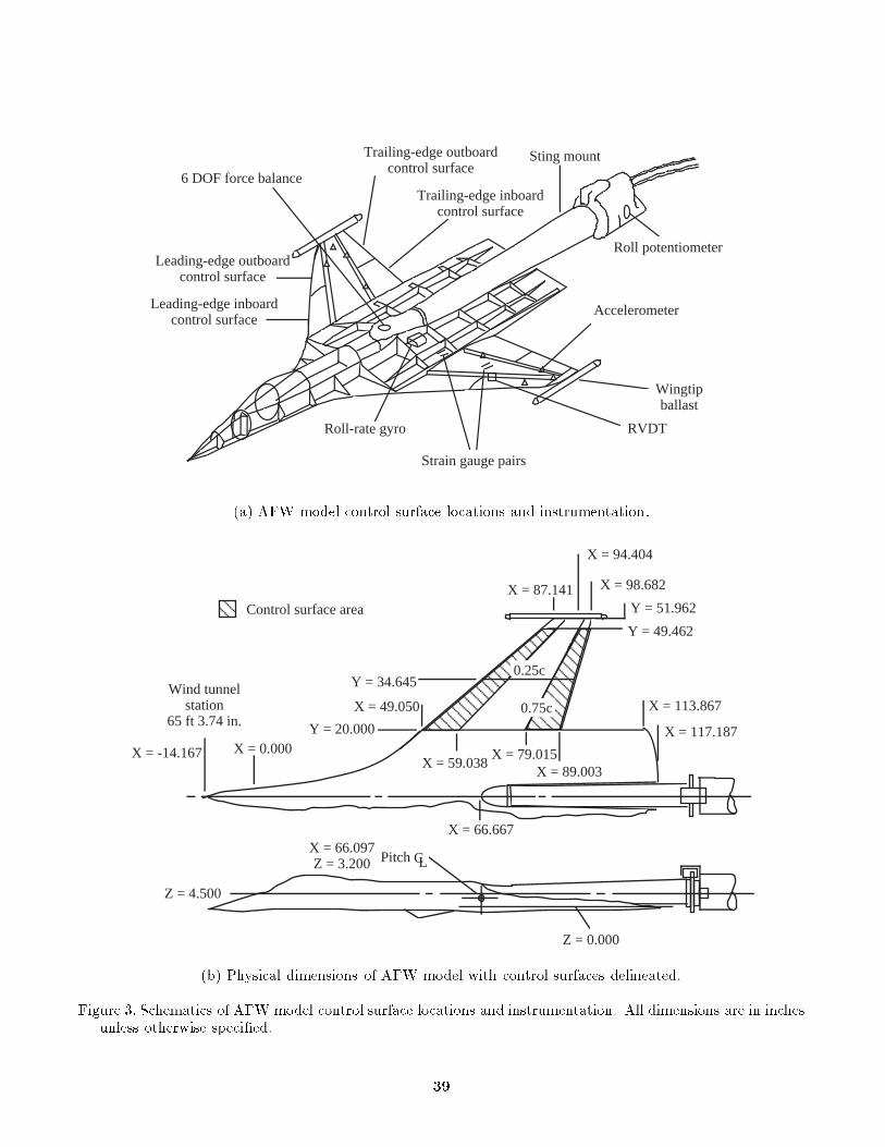
Strain gauge pairs

Leading-edge outboardcontrol surface

Trailing-edge outboardcontrol surface

Leading-edge inboard control surface

Trailing-edge inboardcontrol surface

Roll-rate gyro

Accelerometer

RVDT

6 DOF force balance

Roll potentiometer

Sting mount

Wingtip ballast

(a) AFW model control surface locations and instrumentation.

AAAAAAAAAAAA

AAAAAAAAAAAAAAAAAAAA

X = 0.000

Wind tunnelstation

65 ft 3.74 in. Y = 20.000

X = 49.050

Y = 34.6450.25c

0.75c

Pitch CL

Y = 49.462

X = 87.141Y = 51.962

X = -14.167

X = 94.404

X = 98.682

X = 113.867

X = 117.187

X = 79.015X = 89.003

X = 59.038

X = 66.667X = 66.097Z = 3.200

Z = 0.000

Z = 4.500

AAControl surface area

(b) Physical dimensions of AFW model with control surfaces delineated.

Figure 3. Schematics of AFW model control surface locations and instrumentation. All dimensions are in inchesunless otherwise speci�ed.

39

Control surface

actuators

L-90-12024

Figure 4. Photograph of actuator and attachment to wing.

Y = 32.375

TMLO1

TMLO2

BMLO1

BMLO2

X = 69.80TMLI1

BMLI1

BMLI2

TMLI2

Y = -10.0

Y = -32.375

TMRO1

BMRO1

BMRO2TMRO2

TMRI1BMRI1BMRI2TMRI2

Y = 0.00

Y = 10.0

X/c = 0.5

Strain gauge

Figure 5. AFW strain gauge locations. All dimensions are in inches. (From ref. 7.)

40

AFW wing

Spring element

Hydraulicactuator

Brake

Addedballast

AddedballastPivot

mechanism

Figure 6. Tip-ballast decoupler pylon.

AAAAAAAAAAAAAAAAAAAAAAAAAAAAAAAAAAAAAAAAAAAAAAAAAAAAAAAAAAAAAAAAAAAAAA

data bus

HostCPU

Arrayprocessor(Backup

processor)

Diskstorage

FloatingpointDSP

(Control law processor)

INTEGERDSP

(Real-Time Executor)

Ethernet

SUN WorkstationAA

Analogdigital

conversion

AAAA

Tape

Digital controllersystem

Interfaceelectronics

Power supply

Filter box

Status displaypanelA

AFWsimulation

Discreteout

Analog out

Analog in

AAAAAAA

Patch boxAAA

Operator'sconsoleDisplay

AA

AAAAA

AFW ModelAAAAAAAAAAAAAAAA

AFW model

Figure 7. Schematic of AFW digital controller.

41

δTEO

AFWplantmodel

G2

G3

G1

φ, φ, loads

δTEI

δLEO

Command.

Figure 8. Analysis structure for load e�ectiveness study.

150

-150

-90

-30

30

-210

90

0 .2 .4 .6 .8 1.0

φ

φ.

Time, sec

Rol

l ang

le, φ

, deg

Rol

l rat

e, φ

, deg

/sec

.

(a) tF = 0:58 sec.

0 .2 .4 .6 .8 1.0

AAAAAAAA-6000

-4000

-2000

0

2000

Time, sec

AAAAAA

AAAAAAAAAAAA

AAA

AAAAAAAAAAAAAAAAAAAAAAA

AAAA

AAAAAAAAAA

AAAAAAA

Mδ

Mxx

Mp

Mm

Mom

ents

, in-

lb

(b) Moment contributions for time to roll 90� oftF = 0:58 sec.

Time, sec

-80

-40

0

40

80

120

0 .4 .8 1.2 1.6 2.0

AAAAAAAA

φ

φ.

Rol

l ang

le, φ

, deg

Rol

l rat

e, φ

, deg

/sec

.

(c) tF = 1:8 sec.

AAAAAAAAAA

AAAAAAAA

0 1.6 2.0.4 .8 1.2

AAAAAA

AAAAAAAAAAAAAAAAAAAAA

AAAAAA

AAAAAAAAAAAAA

AA

-2000

-1000

0

1000

2000

Time, sec

Mδ

Mxx

Mp

Mm

Mom

ents

, in-

lb

(d) Moment contributions for time to roll 90� oftF = 1:8 sec.

Figure 9. Simulated roll angle, roll rate, and moments for q = 150 psf with mass eccentricity.

42

AA

AAAAAA

AAAAAAAAA

AAAAAAAAA

AAAAAA

1 2 3

2.0

1.0

3.0

Inte

gral

mom

ents

, in-

lb-s

ec

Mm

Mδ

0

× 103

tF, sec

Figure 10. Simulated pendulum rolling moment and control-surface rolling moment integral values at

q = 150 psf.

BMO BMI TMO TMILoad

Loa

d lim

it, p

erce

nt

Peak incrementalSteady load

0

5

10

15

20

25

30

35

Figure 11. Design model steady load plus peak incremental load.

500

400

300

200

100

0Time, sec

Incr

emen

tal o

utbo

ard

bend

ing

mom

ent,

in-l

b

1.0.5 1.5

+TEO

-LEO

+LEO

-TEO

BASE

Figure 12. Incremental outboard bending moment generated during rolling maneuvers.

43

+

–

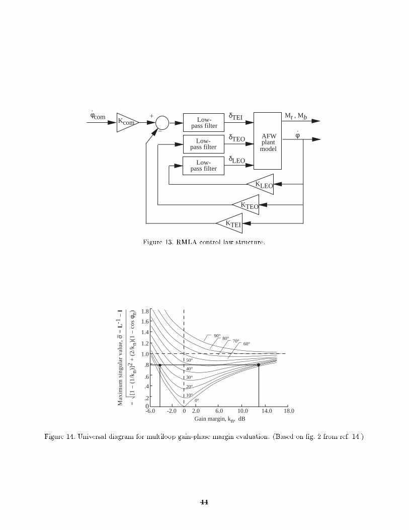
Kcom

AFWplantmodel

Mt , Mb˙ φcom

˙ φ

δTEI

δTEO

δLEO

KTEI

KLEO

KTEO

Low-pass filter

Low-pass filter

Low-pass filter

Figure 13. RMLA control law structure.

Gain margin, kn, dB

0°10°

20°

30°

40°

50°

60°70°

80°90°

-6.0 -2.0 0 2.0 6.0 10.0 14.0 18.0

.2

1.8

1.6

1.4

1.2

1.0

.8

.6

.4

0Max

imum

sin

gula

r va

lue,

σ =

L-1

– I

=

[1

– (1

/kn)

]2 +

(2/

k n)(

1 –

cos

φ n)

Figure 14. Universal diagram for multiloop gain-phase margin evaluation. (Based on �g. 2 from ref. 14.)

44

Dyn

amic

pre

ssur

e, p

sf

20

30

40

50

60

70

80

90

100

200

300

400

500

Open-loop flutter q, tip ballast coupled

29.7 mW (power limit)10.5 mW rotor limit

26.1 mW (10 min time limit above)235 rpm limit, vane angle = 2° (low speed windings)

235 rpm limit (low speed windings)

470 rpm limit (high speed windings)

470 rpm limit, vane angle = 2°

(High speed windings)

RMLA test point with tip ballast coupledRMLA test point with tip ballast decoupledRMLA test point with tip ballast coupled and FSS operating simultaneously

0 .1 .2 .3 .4 .6 .7 .8 .9 1.0 1.1 1.2 1.3.5

Mach number

Figure 15. TDT ight envelope in air with RMLA test points identi�ed.

45

RMLA controller active RTS active RTS holds model at initial trim angle

φL

φcap

Ramp-on/holdcommand with slope = φLon

φc = φcap

φcom

Roll-rate command,

tF

φLφLon

and φLoff

.

tB tcap

Ramp-off commandwith slope = φLoff

Peak hold roll rate

Ramp rates (slopes) for roll-rate command

.

.

.

. ...

....

Figure 16. Roll-rate command structure. (From ref. 10.)

1.4

1.2

1.0 (nominal)

0.8

Roll-ratecommand,

φcom.

Figure 17. Command input scale factors.

46

Rol

l rat

e, d

eg/s

ec

Time, sec

-250

-200

-150

-100

-50

0

50

.50 1.0 1.5

(a) Roll rate.

Rol

l ang

le, d

eg

Time, sec

-50

0

50

100

.50 1.0 1.5

Baseline controlled RMLA controlledTermination of control law

(b) Roll angle.

Incr

emen

tal o

utbo

ard

tors

ion

mom

ent,

in-l

b

Time, sec

-600

-400

-200

0

200

.50 1.0 1.5

(c) Incremental outboard torsion moment. PeakRMLA = 359.6 in-lb; Peak baseline = 495.1 in-lb.

Incr

emen

tal i

nboa

rdto

rsio

n m

omen

t, in

-lb

Time, sec

-2000

-1000

0

1000

.50 1.0 1.5

(d) Incremental inboard torsion moment. PeakRMLA = 747.1 in-lb; Peak baseline = 1565.0 in-lb.

Incr

emen

tal o

utbo

ard

bend

ing

mom

ent,

in-l

b

Time, sec

-1000

-500

0

500

1000

.50 1.0 1.5

(e) Incremental outboard bending moment. PeakRMLA = 638.0 in-lb; Peak baseline = 185.7 in-lb.

Incr

emen

tal i

nboa

rdbe

ndin

g m

omen

t, in

-lb

Time, sec

-1000

-500

0

500

1000

.50 1.0 1.5

(f) Incremental inboard bending moment. PeakRMLA = 403.8 in-lb; Peak baseline = 352.2 in-lb.

Figure 18. RMLA control law A controlled-maneuver loads compared with baseline loads at q = 200 psf.

47

Rol

l rat

e, d

eg/s

ec

Time, sec

-250

-200

-150

-100

-50

50

.50 1.0 1.5

0

(a) Roll rate.

Rol

l ang

le, d

eg

Time, sec

-50

0

50

100

.50 1.0 1.5

Baseline controlled RMLA controlledTermination of control law

(b) Roll angle.

Incr

emen

tal o

utbo

ard

tors

ion

mom

ent,

in-l

b

Time, sec

-600

-400

-200

200

400

.50 1.0 1.5

0

(c) Incremental outboard torsion moment. PeakRMLA = 265.6 in-lb; Peak baseline = 495.1 in-lb.

Incr

emen

tal i

nboa

rdto

rsio

n m

omen

t, in

-lb

Time, sec

-2000

-1000

0

1000

.50 1.0 1.5

500

-500

-1500

(d) Incremental inboard torsion moment. PeakRMLA = 885.8 in-lb; Peak baseline =1565.0 in-lb.

Incr

emen

tal o

utbo

ard

bend

ing

mom

ent,

in-l

b

Time, sec

-400

-200

0

400

600

.50 1.0 1.5

200

(e) Incremental outboard bending moment. PeakRMLA = 259.5 in-lb; Peak baseline = 185.7 in-lb.

Incr

emen

tal i

nboa

rdbe

ndin

g m

omen

t, in

-lb

Time, sec

-200

200

400

800

1000

.50 1.0 1.5

600

0

(f) Incremental inboard bending moment. PeakRMLA = 408.6 in-lb; Peak baseline = 352.2 in-lb.

Figure 19. RMLA control law B controlled-maneuver loads compared with baseline loads at q = 200 psf.

48

TMO TMI BMO BMI0

1000

2000Pe

ak in

crem

enta

l lo

ads,

in-l

b

Baseline

RMLA A

-52.3%

14.7%

243.6%-27.4%

(a) tF = 0:66 sec using control law A.

TMO TMI BMO BMI0

1000

2000

Peak

incr

emen

tal

load

s, in

-lb

Baseline

RMLA B-43.4%

39.7%

16.0%-46.4%

(b) tF = 0:645 sec using control law B.

Figure 20. Change in peak incremental loads for two RMLA-controlled maneuvers with performance timessimilar to the baseline control law at q = 200 psf.

49

.675 .695 .805-100

-50

0

50

100

Performance time, sec

TMO TMI BMO BMI

Stea

dy-s

tate

load

, per

cent

(a) Control law A at q = 150 psf.

.635 .660 .770

Performance time, sec

-100

-50

0

50

100TMO TMI BMO BMI

Stea

dy-s

tate

load

, per

cent

(b) Control law A at q = 200 psf.

.635 .660 .770-100

-50

0

50

100

Stea

dy-s

tate

load

, per

cent

Performance time, sec

TMO TMI BMO BMI

(c) Control law A at q = 250 psf.

.675 .695 .805-100

-50

0

50

100

Performance time, sec

TMO TMI BMO BMI

Stea

dy-s

tate

load

, per

cent

(d) Control law B at q = 150 psf.

.635 .660 .770-150

-100

-50

0

50

100

Performance time, sec

TMO TMI BMO BMI

Stea

dy-s

tate

load

, per

cent

(e) Control law B at q = 200 psf.

.635 .660 .770-150

-100

-50

0

50

100

Performance time, sec

TMO TMI BMO BMI

Stea

dy-s

tate

load

, per

cent

(f) Control law B at q = 250 psf.

Figure 21. Percent change in peak incremental load of baseline loads and RMLA-controlled loads relative to

steady-state loads at beginning of maneuver.

50

Performance time, sec

0

10

20

30

40

50

60

Loa

d lim

it, p

erce

nt

.615 .645 .740

(a) Torsion moment outboard.

Control law peak incremental load

Steady loadBaseline peak incremental load

Performance time, sec

0

10

20

30

40

50

60

Loa

d lim

it, p

erce

nt

.615 .645 .740

(b) Torsion moment inboard.

Performance time, sec

Loa

d lim

it, p

erce

nt

0

10

20

30

40

50

60

.615 .645 .740

(c) Bending moment outboard.

Performance time, sec

0

10

20

30

40

50

60

Loa

d lim

it, p

erce

nt

.615 .645 .740

(d) Bending moment inboard.

Figure 22. Steady load plus peak incremental relative to static load limits for baseline control law and controllaw A at q = 200 psf.

51

Performance time, sec

0

10

20

30

40

50

60

Loa

d lim

it, p

erce

nt

.615 .645 .740

(a) Torsion moment outboard.

Control law peak incremental load

Steady loadBaseline peak incremental load

Performance time, sec

0

10

20

30

40

50

60

Loa

d lim

it, p

erce

nt

.615 .645 .740

(b) Torsion moment inboard.

Performance time, sec

Loa

d lim

it, p

erce

nt

0

10

20

30

40

50

60

.615 .645 .740

(c) Bending moment outboard.

Performance time, sec

0

10

20

30

40

50

60

Loa

d lim

it, p

erce

nt

.615 .645 .740

(d) Bending moment inboard.

Figure 23. Steady load plus peak incremental relative to static load limits for baseline control law and controllaw B at q = 200 psf.

52

Performance time, sec

Cha

nge,

per

cent

.55 .65 .75 .85

-60

-40

-20

0

-80

(a) Control law A, torsion moment outboard.

150 psf, experimental

250 psf, experimental150 psf, analytical250 psf, analytical

Cha

nge,

per

cent

Performance time, sec.55 .65 .75 .85

-60

-40

-20

0

-80

(b) Control law B, torsion moment outboard.

.55 .65 .75 .85

-60

-40

-20

0

-80

Performance time, sec

Cha

nge,

per

cent

(c) Control law A, torsion moment inboard.

Cha

nge,

per

cent

.55 .65 .75 .85

-60

-40

-20

0

-80

Performance time, sec

(d) Control law B, torsion moment inboard.

Figure 24. Analytical and experimental incremental load reductions.

53

0 .5 1.0 1.5 2.0

2.0

-2.0

-4.0

-6.0

-8.0

0

Time, sec

δ LE

OR

, deg

(a) LEO control surface de ection commanded by RMLA control law B.

6.0

4.0

2.0

0

-2.0

-4.0

-6.0

-8.00 .5 1.0 1.5 2.0

Time, sec

δ TE

I R, d

eg

(b) TEI control surface de ection commanded by RMLA control law B.

.3

.2

0

.1

-.4

-.1

-.2

-.3

0 .5 1.0 1.5 2.0Time, sec

δ TE

OR

, deg

(c) TEO control surface de ection commanded by utter suppression control law.

Figure 25. Control surface activity during rolling maneuver with simultaneous implementation of RMLA andFSS control laws.

54

0

-10

-20

-30

-40

-50

10

0 2 41 3Time, sec

Rol

l rat

e, d

eg/s

ec

SimulatedFree fall

(a) Comparison of simulated roll rate with experi-mental free-fall roll rate at q = 150 psf.

Rol

l ang

le, d

eg

0 1 2 3 4

40

-20

0

20

60

80

100

Time, sec

SimulatedFree fall

(b) Comparison of simulated roll angle with experi-mental free-fall roll angle at q = 150 psf.

Time, sec0 1 2 3 4

-2000

0

-1800

-1600

-1200

-1000

-1400

Lef

t inb

oard

tors

ion

mom

ent,

in-l

b SimulatedFree fall

(c) Comparison of simulated left inboard torsion mo-ment with experimental free-fall inboard torsionmoment at q = 150 psf.

Time, sec0 1 2 3 4

100120

140

160

180

200220

0

Lef

t out

boar

d to

rsio

nm

omen

t, in

-lb

SimulatedFree fall

(d) Comparison of simulated left outboard torsionmoment with experimental free-fall outboard tor-sion moment at q = 150 psf.

0 1 2 3 4

-1800

-1600

-1400

-1200

-1000

-2000

Time, sec

Rig

ht in

boar

d to

rsio

nm

omen

t, in

-lb

SimulatedFree fall

(e) Comparison of simulated right inboard torsionmoment with experimental free-fall inboard tor-sion moment at q = 150 psf.

240

280

320

360

400

10 2 3 40

Time, sec

Rig

ht o

utbo

ard

tors

ion

mom

ent,

in-l

b

SimulatedFree fall

(f) Comparison of simulated right outboard torsionmoment with experimental free-fall outboard tor-sion moment at q = 150 psf.

Figure 26. Comparison of simulated and free-fall data.

55

6000

5200

4400

4800

5600

0 1 2 3 40

Time, sec

Lef

t inb

oard

ben

ding

mom

ent,

in-l

b

SimulatedFree fall

(g) Comparison of simulated left inboard bendingmoment with experimental free-fall inboard bend-ing moment at q = 150 psf.

400

500

600

700

0 1 2 3 4

800

0

Time, sec

Lef

t out

boar

d be

ndin

gm

omen

t, in

-lb

SimulatedFree fall

(h) Comparison of simulated left outboard bend-ing moment with experimental free-fall outboardbending moment at q = 150 psf.

4000

0 1 2 3 4

4500

3500

0

Time, sec

Rig

ht in

boar

d be

ndin

gm

omen

t, in

-lb

5000SimulatedFree fall

(i) Comparison of simulated right inboard bend-ing moment with experimental free-fall outboardbending moment at q = 150 psf.

500

600

700

800

0 1 2 3 4

900

Time, sec

Rig

ht o

utbo

ard

bend

ing

mom

ent,

in-l

b

0

SimulatedFree fall

(j) Comparison of simulated right outboard bend-ing moment with experimental free-fall outboardbending moment at q = 150 psf.

Figure 26. Concluded.

56

REPORT DOCUMENTATION PAGEForm Approved

OMB No. 0704-0188

Public reporting burden for this collection of information is estimated to average 1 hour per response, including the time for reviewing instructions, searching existing data sources,gathering and maintaining the data needed, and completing and reviewing the collection of information. Send comments regarding this burden estimate or any other aspect of thiscollection of information, including suggestions for reducing this burden, to Washington Headquarters Services, Directorate for Information Operations and Reports, 1215 Je�ersonDavis Highway, Suite 1204, Arlington, VA 22202-4302, and to the O�ce of Management and Budget, Paperwork Reduction Project (0704-0188), Washington, DC 20503.

1. AGENCY USE ONLY(Leave blank) 2. REPORT DATE 3. REPORT TYPE AND DATES COVERED

October 1994 Technical Paper

4. TITLE AND SUBTITLE

Active Load Control During Rolling Maneuvers

6. AUTHOR(S)

Jessica A. Woods-Vedeler, Anthony S. Pototzky, and Sherwood T. Hoadley

7. PERFORMING ORGANIZATION NAME(S) AND ADDRESS(ES)

NASA Langley Research CenterHampton, VA 23681-0001

9. SPONSORING/MONITORING AGENCY NAME(S) AND ADDRESS(ES)

National Aeronautics and Space AdministrationWashington, DC 20546-0001

5. FUNDING NUMBERS

WU 505-63-36-01

8. PERFORMING ORGANIZATION

REPORT NUMBER

L-17053

10. SPONSORING/MONITORING

AGENCY REPORT NUMBER

NASA TP-3455

11. SUPPLEMENTARY NOTES

Woods-Vedeler and Hoadley: Langley Research Center, Hampton, VA; Pototzky: Lockheed Engineering &Sciences Company, Hampton, VA.

12a. DISTRIBUTION/AVAILABILITY STATEMENT 12b. DISTRIBUTION CODE

Unclassi�ed{Unlimited

Subject Category 05

13. ABSTRACT (Maximum 200 words)

A rolling maneuver load alleviation (RMLA) system has been demonstrated on the Active Flexible Wing(AFW) wind tunnel model in the Langley Transonic Dynamics Tunnel (TDT). The objective was to developa systematic approach for designing active control laws to alleviate wing loads during rolling maneuvers. TwoRMLA control laws were developed that utilized outboard control-surface pairs (leading and trailing edge) tocounteract the loads and that used inboard trailing-edge control-surface pairs to maintain roll performance.Rolling maneuver load tests were performed in the TDT at several dynamic pressures that included twobelow and one 11 percent above the open-loop utter dynamic pressure. The RMLA system was operatedsimultaneously with an active utter suppression system above open-loop utter dynamic pressure. At alldynamic pressures for which baseline results were obtained, torsion-moment loads were reduced for both RMLAcontrol laws. Results for bending-moment load reductions were mixed; however, design equations developed inthis study provided conservative estimates of load reduction in all cases.

14. SUBJECT TERMS 15. NUMBER OF PAGES

Aircraft; Rolling maneuver; Wind tunnel; Dynamic loads; Control system 59

16. PRICE CODE

A0417. SECURITY CLASSIFICATION 18. SECURITY CLASSIFICATION 19. SECURITY CLASSIFICATION 20. LIMITATION

OF REPORT OF THIS PAGE OF ABSTRACT OF ABSTRACT

Unclassi�ed Unclassi�ed Unclassi�ed

NSN 7540-01-280-5500 Standard Form 298(Rev. 2-89)Prescribed by ANSI Std. Z39-18298-102