Project ID: NTC2016-MU-R-04

ACTIVE BOTTLENECK MANAGEMENT ON FREEWAYS THROUGH CONNECTED VEHICLES

by Mecit Cetin mcetin@odu.edu Ehsan Beheshtitabar ebehe001@odu.edu Reza Vatani Nezafat rvata001@odu.edu Transportation Research Institute (TRI) Department of Civil & Environmental Engineering Old Dominion University and George F. List gflist@ncsu.edu Elizabeth Williams egwilli4@ncsu.edu North Carolina State University Department of Civil, Construction, and Environmental Engineering for National Transportation Center at Maryland (NTC@Maryland) OCTOBER 2017

iii

ACKNOWLEDGEMENTS The project was funded by the National Transportation Center @ Maryland (NTC@Maryland), one of the five National Centers that were selected in this nationwide competition, by the Office of the Assistant Secretary for Research and Technology (OST-R), U.S. Department of Transportation (US DOT). DISCLAIMER The contents of this report reflect the views of the authors, who are solely responsible for the facts and the accuracy of the material and information presented herein. This document is disseminated under the sponsorship of the U.S. Department of Transportation University Transportation Centers Program in the interest of information exchange. The U.S. Government assumes no liability for the contents or use thereof. The contents do not necessarily reflect the official views of the U.S. Government. This report does not constitute a standard, specification, or regulation.

1

TABLE OF CONTENTS

EXECUTIVE SUMMARY .......................................................................................................... 2 1.0 INTRODUCTION............................................................................................................. 3

1.1 REPORT OVERVIEW ....................................................................................................... 4 2.0 BACKGROUND ON STUDY SITE................................................................................ 4 3.0 LITERATURE REVIEW ................................................................................................ 6

3.1 TUNNEL TRAFFIC MANAGEMENT AND SAFETY ................................................... 6 3.2 ACTIVE TRAFFIC MANAGEMENT FOR TRAFFIC BREAKDOWN AND

CAPACITY DROP PHENOMENA ................................................................................. 10 3.3 MICROSIMULATION CALIBRATION ........................................................................ 14 3.4 SYSTEM STATE ESTIMATION FROM CONNECTED VEHICLE AND PROBE

VEHICLE DATA ............................................................................................................. 16 4.0 FIELD DATA COLLECTION ...................................................................................... 19

4.1 PER VEHICLE RECORD (PVR) DATA ........................................................................ 19 4.2 PROBE VEHICLE DATA ............................................................................................... 20 4.3 INRIX SPEED DATA ...................................................................................................... 22 4.4 WAVETRONIX DATA ................................................................................................... 23 4.5 VIRGINIA DEPARTMENT OF TRANSPORTATION VIDEO FEEDS ....................... 25

5.0 VISSIM MICRO SIMULATION MODEL .................................................................. 26 5.1 THE VISSIM MODEL FEATURES ................................................................................ 26

5.1.1 LOOK AHEAD DISTANCE PARAMETER .......................................................... 27 5.1.2 CAR FOLLOWING PARAMETERS ...................................................................... 27 5.1.3 TIME HEADWAY DISTRIBUTION ...................................................................... 27 5.1.4 CAR FOLLOWING VARIATION .......................................................................... 28 5.1.5 CRAWL SPEEDS ..................................................................................................... 28

6.0 CALIBRATION .............................................................................................................. 28 7.0 IMPACTS OF CONNECTED VEHICLES ................................................................. 31

7.1 CONNECTED VEHICLES IN MIXED TRAFFIC ......................................................... 32 7.1.1 Analysis of Look Ahead Distance ............................................................................ 32

7.2 VARIABLE SPEED CONTROL IN A SAG CURVE..................................................... 34 7.2.1 Variable Speed Limit Control Strategy for Sag Curves............................................ 34

8.0 CONCLUSION AND FUTURE WORKS .................................................................... 45 REFERENCES ............................................................................................................................ 47

2

EXECUTIVE SUMMARY

This study is focused on bottleneck formations on freeways and how utilization of connected vehicles could improve the traffic flow. Bottlenecks are restrictions points along a freeway that have lower capacities than their upstream segments. In this study, the focus is on sag curves and tunnels. Using the Hampton Roads Bridge Tunnel (HRBT) in Norfolk as the study site, the team developed several models to capture traffic behavior through a tunnel. An extensive literature review is conducted to document previous findings on traffic flow and control at sag curves and tunnels. It also included relevant active traffic management strategies, the use of connected vehicles to estimate the state of system, calibration of microsimulation models, and the traffic management practices for tunnels. A number of studies has been completed in the past on various technologies to manage the congestion within tunnels and strategies to estimate and improve the traffic conditions within a tunnel. Managing the length of queues and the duration of bottlenecks in the context of tunnel traffic have been investigated as well. In this project, traffic data from fixed sensors and probe vehicle data along the HRBT corridor are collected and analyzed to characterize the pertinent traffic flow phenomena. Evolution of congestion patterns and how they impact the throughput are investigated. The data are then used to calibrate a microscopic simulation model developed in VISSIM. After calibrating the model created for the HRBT, the importance of the downstream observability in absorbing shockwaves and preventing bottleneck formation within the tunnel are investigated. Reduced downstream observability (i.e., ability of the driver to observe additional vehicles ahead) due to restricted tunnel geometry is regarded as an important factor in shockwave and phantom jam generation within a tunnel which lead to bottleneck formations and a lower throughput. For testing the effect of higher downstream observability in reducing the bottleneck formation, simulation scenarios are implemented, where a percentage of cars within the traffic is assumed to have higher downstream observability. These cars are assumed to be probe cars which have higher downstream observability because of connectivity to other probe cars and the infrastructure. The results of the tests show significant travel time reductions and capacity increase at the tunnel. The research team also investigated traffic control options that could improve the throughput and delays in a typical sag curve. In particular, a control strategy based on the variable speed limit (VSL) principles is developed and simulated using an advanced car following model. Traffic flow along a sag curve is simulated using the intelligent driver model (IDM), a time-continuous car-following model. A feedback control algorithm is developed for adjusting the approach speeds of connected vehicles (CVs) so that the throughput of the sag curve is maximized. Depending on the traffic density at the sag curve, adjustments are made to the speeds of the CVs. A simulation-based optimization method using a meta-heuristic algorithm is employed to determine the critical control parameters. Various market penetration rates for CVs are also considered in the simulations. Even at relatively low market penetration rates (e.g., 5-10 %), significant improvements in travel times and throughput are observed. Additional details of this model are presented in the report.

3

1.0 INTRODUCTION

Bottlenecks along freeways are locations where the roadway capacity is reduced in comparison to their upstream segments. These changes in capacity are often the result of lane drops, tunnels, sag curves, and other constrictions at which traffic demand exceeds capacity. To minimize delays along the network, it is imperative that the capacity through these points of constriction be maximized while mitigating the effects of incidents or irregular/turbulent traffic flow. Freeways regularly face bottlenecks where the capacity can drop by 10-20%. Various Active Traffic Management (ATM) strategies for freeways have been developed to avoid such capacity drops. These include adaptive ramp metering, dynamic lane use, and dynamic speed limits. These strategies have historically required the installation of field equipment, such as a Dynamic Message Signs (DMSs), to regulate traffic or advise drivers about speed limits. Due to the high cost of installing, maintaining, and operating such field equipment, ATM strategies have been deployed only at a limited number of locations. With the emergence of Connected Vehicles (CVs) or probe vehicle technology, there exists new opportunities to dynamically control traffic at a fraction of cost required for traditional ATM deployments. There has been increasing use of computer simulation models used to study the performance of transportation networks. These tools are especially crafted to deal with the details of network design and operation. They also allow for future traffic conditions to be assessed as well as the impacts of changes in the network to be calculated. It is imperative that the simulation model be properly calibrated so that the traffic conditions are accurately represented. Much research has been completed regarding the calibration of simulation models along basic freeway networks and arterials. Despite this progress, it is apparent that calibrating simulation models for driving behavior through tunnels has been limited. A tunnel serves as a critical link of the transportation network and especially at the site selected for investigation in this project. Tunnels in rural and urban areas facilitate traffic flow through waterways where bridge construction is not feasible. Given the nature of tunnels, it is imperative that tunnels be cleared of congestion to maximize the safety of the system. Although incidents that occur on open roadways are dangerous, the same type of incidents can be disastrous in tunnels. When an accident occurs within a tunnel, it becomes incredibly difficult for vehicles to exit the tunnel. This backup often causes secondary accidents. Because of this, it is important that congestion and incidents be cleared as soon as possible. Tunnels tend to face other significant challenges as compared to other types of facilities in the transportation network. Tunnel performance is affected by the physical design of the facility. Roadway characteristics such as striping, painting, and lighting, play more critical roles affecting the tunnel capacity as compared to basic freeway segments. Because of these features, it is challenging to calibrate a simulation model that accurately depicts the performance of these facilities. In addition, it is essential to understand the characteristics of traffic patterns and current mitigation strategies for bottlenecks and extensive queues on freeways and tunnels. Current practices include speed harmonization and ramp metering to control vehicle density. Others seek to minimize the

4

length of queues and the duration of bottlenecks to reduce overall delay in the system. These strategies aim to maximize the safety along roadways, especially in tunnels. This project includes these notions in the development of a connected-vehicle policy and tool for mitigating the effects of bottlenecks.

1.1 REPORT OVERVIEW

The remainder of this report is organized as follows. Section 2 presents an overview of the selected study site, the HRBT corridor. The following sections examine existing literature and the available data for this project. The methodology and development of a VISSIM microsimulation model are provided in Section 5, followed by the calibration of the model in Section 6. Section 7 describes the proposed impact of the CVs in the field. The final section provides a summary and conclusions for the future research in this domain.

2.0 BACKGROUND ON STUDY SITE

The I-64 Hampton Roads Bridge Tunnel in Virginia was selected as the site of interest for this project. This facility has a roadway in both the eastbound and westbound direction. In each direction, there is a bridge section followed by a tunnel then another bridge before reaching the land. The tunnel itself carries traffic on two 12-feet long freeway lanes. The speed limit along this section is 55 mph for a length of 3.6 miles (5.6 km). The 1.6-mile tunnel can be divided into three sections, based on three different grades. The bridge section enters a downhill with a grade of 4% for a total downhill length of 3,046 feet. The downhill section is followed by a relatively straight section with length of 3,146 feet which has a slope of +0.5%. This section is followed by the upgrade section which has a slope of +4% and a length of 2,526 feet. Figure 2.1 illustrates the discussed profile.

Figure 2.1: The HRBT longitudinal profile as created in VISSIM for the simulations This facility was selected because it is along a major route in the region and congestion is regularly experienced in the peak hours. The congestion tends to result in the tunnel because of the sag curve in the longitudinal profile. Cetin et al. (2014) showed that when congestion is formed inside the tunnel, the throughput of the tunnel is significantly less than when the congestion is formed outside the tunnel. In addition, Cetin et al. (2014) recognized that bottlenecks form in all the evening

5

observations and in nearly all the evening peak hour bottlenecks observations (28 out of 32 observations). It is important to note that the congestion is likely to be affected by the sunshine as it is directly towards the driver’s windshield. The relationship between the sun and the driver causes a percentage of the drivers to slow down in addition to the effects of the sag curve. Inside the tunnel, vehicles have varying characteristics in terms of the following driving behavior parameters.

• Desired speed of traveling • Desired time headway to the car in front • Kinematics of the vehicles (power to mass ratio) and acceleration rates

From the videos recorded within the tunnel, it is observed that large trucks can have headways as large as 14 seconds. In the left lane where only cars are permitted to travel, the desired time headways are more homogenous and in a narrower distribution, resulting in 20% higher throughput when compared to the right lane. These differences between vehicles are present in any highway but can have more significant implications in a tunnel sag curve as they lead to shockwave formation, bottleneck formation and sometimes phantom jams. During both the AM and PM peak hours, there is a high demand leading to a queue formation at the upstream of the tunnel. This queue of vehicles has a bottleneck at the entrance of the tunnel where cars start to follow with a larger headway inside the tunnel. The vehicles also have larger variation in the gap when following inside a tunnel (Anuar, Habtemichael et al. 2015). In order to prevent bottlenecks inside the tunnel and to obtain a higher throughput from the tunnel, formation and disruptions of potential shockwaves within the tunnel needs be prevented.

6

3.0 LITERATURE REVIEW

In the proceeding sections, a literature review on the previous research which is related to the research of this report are presented. They include tunnel traffic, traffic management in freeways and traffic control for congestion management.

3.1 TUNNEL TRAFFIC MANAGEMENT AND SAFETY

Tunnels have been the focus of research due to the specific traffic conditions which they provide. Yan and Lam (1996) studied the use of tolls to reduce queues and congestion in tunnels in Hong Kong. During the course of their investigation, they determined procedures to find the optimal toll values to effectively mitigate congestion. Jha et al. (1995) investigated the effectiveness of lane control signals in order to address bottlenecks that occur because of freeway geometry or the presence of a lane closure. Ben-Akiva et al. (2003) evaluated various transportation control strategies at tunnel entrances including lane control signals, variable speed limit signs, in-vehicle route guidance, and portal signals. Hongke et al. (2007) analyzed highway tunnel traffic and suggested strategies for highway tunnel traffic control and guidance. Manser and Hancock (2007) analyzed the impact that different visual patterns on the tunnel walls had on drivers’ speed and control. Lin et al. (2013) examined two one-way tunnels in order to understand capacity of the tunnel. Spiliopoulou et al. (2010) proposed a real-time merging traffic control system for toll plazas. The authors asserted that the same control strategy can be applied to traffic through tunnels. Song et al. (2010) determined an alternative model using an Elman Neural Network, a form of iterative feedforward network, to predict traffic flows in tunnels. Researchers have been investigating the safety characteristics for vehicles in tunnels. Vashitz et al. (2007) simulated tunnel driving in order to determine the impact of information displays on the travelers’ experience. Cascetta et al. (2011) investigated the use of automated speed section enforcement system in tunnels. Calvi et al. (2012) performed a driving simulation study to determine the effect tunnels have on the driving experience. Liao et al. (2012) studied different traffic management policies for the Hsueh-Shan Tunnel, the fifth largest tunnel in the world. Wang et al. (2013) provided strategies to prevent fire-related fatalities in the infrastructure of tunnels. Guo et al. (2013) presented the use of tunnel units to address disasters within tunnels. Patnaik et al. (2014) proposed an automatic traffic control and monitoring system for single lane tunnels. The authors suggested the use of a microcontroller that controls the entire system in terms of maintaining a desired level of density. Yeung and Wong (2014) analyzed vehicular movements in the tunnel including driver behavior, speed, and headways. Tan and Gao (2015) promoted new methods in order to manage both the air quality and congestion within a tunnel.

Through the past decades numerous research projects were dedicated to preventing congestion within tunnels and improving the safety of tunnel traffic. Golden River Technologies (Herkt, 1990)

7

were among the first manufacturers to release technologies to manage traffic within tunnels. The aim of their product was not to increase the network’s capacity, but rather relieve the urban system from traffic burdens. This means that the installed technology would work to manage densities within tunnels. The system the company released was two-fold. First, the product utilized an algorithm to detect vehicles in and approaching the tunnels, then use a simulation model to calibrate the traffic control system. Koshi et al. (1992) analyzed the impact that sag vertical curves had on drivers’ speeds and other behaviors within tunnels. They observed that speeds reduce when passing through a sag vertical curve where as there is an insufficient acceleration on the part of the drivers to maintain speed in the positive change to roadway grade due to the increase in gradient in the uphill of the sag curve. Their study discovered that drivers also reduce speed prior to entering a tunnel. Drivers adjust their car following behavior to accommodate for the congestion in a new car following style called by the authors as the congestion car following and gradually resume normal car following behavior when exiting the queue when the time in queue was a little less than 10 minutes. If the time spent in a queue is longer than 1 minutes, the drivers become less sensitive to these parameters. Another interesting point presented in this research was that, with increasing traffic volume, more vehicles tend to use the medium lane (passing lane). A percentage of approximately 60 percent of vehicles in a two-lane section shift to the median lane when the volume approaches the level of 3,000 pcu/h/2 lanes. This would mean that the volume of the median lane is close to 2000 pcu/h/lane which is close to the capacity of that lane. In this scenario even faster vehicles are caught in the median lane platoon. When this platoon is passing a sag curve, the leading vehicles have a slight speed reduction because of the gradient increase and lack of required acceleration operation. This leads to a negative moving shockwave amplifying as its propagating backwards which can result in the complete stop at the tail of the platoon. In tunnels, the speed reduction of vehicles in a platoon head also occurs at the immediate downstream point from the tunnel entrance. This is probably in part because of the psychological impacts that the dark and narrow atmosphere of the tunnel has on many drivers. The higher the percentage of vertical sag curves within a tunnel, the higher the speed reduction prior and in the sag curve of the tunnel, the less tunnel throughput and the more headway between vehicles traveling through it. Jha et al. (1995) investigated the effectiveness of lane control signals, especially in and around tunnels. The authors utilized simulation experiments to conclude that lane control signals extend merge areas but may cause capacity underutilization. Therefore it is possible that lane control signals can increase overall travel times. In conclusion, Jha et al. emphasized the tradeoff between safety and travel times. Ben-Akiva et al. (2003) evaluated freeway control strategies including lane control signs, variable speed limit signs, portal signals at tunnel entrances and in-vehicle route guidance. Their aim was to determine features to incorporate on the Central Artery/Tunnel project in Boston. This project case study was routing through the Ted Williams Tunnel. The team compared the use of lane control signals, variable speed limit signs and route diversion technologies. It was determined that lane control signals and variable speed limit signs increased the travel time in this network while the route diversion had mixed results.

8

Hongke et al. (2007) used simulation in order to determine strategies for the traffic control and guidance within tunnels. The authors first described characteristics of why the tunnel environment is dangerous, especially with the presence of congestion or incidents. These characteristics include brightness, low-intensity lighting and poor air quality environments within the tunnels. Given these conditions, their research aimed to set parameters to control access, speed, lane, and highway network control. Using this information, the team created a simulation model that was able to account for normal operating conditions, congestion, accidents, and fire. Lin et al. (2013) examined tunnel capacity in two one-way tunnels. The free flow speed decreased upstream of the tunnel entrance. The speeds increase in the first 0.2 miles within the tunnel, but would then gradually decrease before stabilizing within the tunnel. Although the drops in speed were around 2 mph, the speed difference is enough to cause obvious changes in capacity. Song et al. (2010) determined an alternative method to predict traffic flows on tunnels on expressways using an Elman Neural Network. An Elman Neural Network is a dynamic recurrent neural network that has the ability to adapt to time-varying characteristics. Using this model, traffic travelling through a tunnel was simulated. Yu et al. (2010) carried a different approach by concentrating their efforts on the development of a traffic flow safety zone algorithm and an algorithm regarding abnormal data detection. Using these procedures, the authors were able to determine the accepted error in detection equipment in tunnels. As a result, traffic volume-time occupancy in tunnels can be better determined. Liao et al. (2012) sought to determine the most effective traffic management policies for the Hsueh-Shan Tunnel. Because this tunnel is the fifth largest tunnel in the world, it is imperative that traffic congestion and incidents be managed effectively. The authors investigated the use of ramp control, opening of shoulder lane, variable message signs, and combinations of the previous strategies. After performing simulation runs, it was concluded that the use of ramp control, variable message signs, and shoulder lane being opened provide the greatest reduction in the queue length. In addition, the presence of ramp and access controls had the lowest density of vehicles. Guo et al. (2013) presented the use of tunnel units on highways in China. The authors describe a state in which there are many long tunnels and adjoining tunnels. Due to the proximity of the tunnels, it is imperative that disasters and traffic control be managed for these groups of tunnels. The authors suggest that the coordination of these tunnels allow for improved plans for disaster prevention and rescue as well as improved traffic conditions. Patnaik et al. (2014) proposed a traffic control system to monitor the traffic density in single lane tunnels. The authors suggest the use of a Microcontroller (ARM Cortex-M0) to complete this task. As a conclusion to this project, they found that their proposed system is able to dynamically monitor traffic density as well as indicate blockages and incidents within single lane tunnels. Yeung and Wong (2014) considered the vehicular movements inside a tunnel. They discovered that drivers perceived a higher risk in a tunnel and have the tendency to drive more cautiously in tunnels. Their findings revealed that road tunnels are superior in the aspect of safety but have less throughput capacity. The study concluded that speed is a key factor on headway, with headways

9

being shorter in the fast lane of the tunnel. Inside the tunnel, headways were recorded greater than while on the open road, specifically on a leader–following composition of HGV-car. The combination of larger headways and lower speeds through tunnels, traffic capacity is contained within the tunnel. Manser and Hancock (2007) used simulation in order to determine if different visual patterns on tunnel walls impacted drivers’ ability to maintain a speed and control. They conducted a trial in which participants faced simulation of driving through tunnels with the thickness of stripes changing, stripes of the same size, and no stripes present on the tunnel walls. Through this study, it was determined that the visual marking on the walls had a significant impact on speeds. While some visual patterns promoted slower speeds, others encouraged acceleration. Liu et al. (2010) investigated different fire scenarios in tunnels given the level of congestion in the tunnel, the tunnel grade, and smoke migration within the tunnel. They used these different parameters to determine different emergency actions that would need to be taken for smoke to be extracted. According to this study with congestion levels increasing, the speed of the traffic decreases. When this occurs, the airflow in the tunnel decreases. This makes a more dangerous condition for smoke in the tunnel’s air. Cascetta et al. (2011) studied the impact of automated section speed enforcement system on the traffic flow patterns, particularly in tunnels and found that there were lower free-flow speeds. Calvi et al. (2012) created the CRISS Driving Simulation Study. This study aimed at analyzing the participants’ driving experience through tunnels. In their research, they tested a group of twenty drivers to drive in an 8500m driving simulation in a highway scenario for making comparison between driving with tunnels and without tunnels. The research stated that from 150 meters before the tunnel entrance, the driver attention would be focused on the tunnel entrance. This means drivers almost neglect all the information provided on signs located closely at the portal. The results indicated a speed reduction inside tunnels by more than 60% of drivers. Drivers also had less measured pathological discomfort when driving in the tunnel. This could be caused by a less need and action of the drivers for correcting their trajectories. It was suspected that the tunnel provides the drivers with a sort of guidance for their trajectory represented by the lateral walls of the tunnel. In summary, the research showed that drivers tend to move towards the center while driving in the tunnel and there are indications of drivers having greater focus within the tunnel. However, speeds of drivers tend to be lower. Vashitz et al. (2007) simulated the driving experience of a tunnel. During the simulations, the drivers were provided a highly or minimal informative display. The results show that the highly informative displays had corresponding improvements in speed and a decline in lane stability. The research asserts that the change in lane stability is related to the informative delays being distracting. However, the highly informative speeds were associated with boredom and anxiety. Wang et al. (2013) discussed the difficulties of fires within tunnels. The authors explain the danger of vehicles heading towards the fire within the tunnel whom are unable to easily turn around. This means that there is little chance to escape the fire. As a solution, they encouraged the use of an extended left repair road, a safety tunnel at the bottom of the main tunnel, refuge holes, and parallel pilot tunnels to separate vehicles from the fire.

10

Tan and Gao (2015) utilized the traffic control to mitigate congestion and improve the air quality within tunnels. The authors used the aerodynamics of vehicles within tunnels to disperse pollutants in the air and maintain a steady-state flow. The use of an optimal time-of-day ramp metering and mainline inlet traffic control model was developed using non-linear programming techniques to achieve these goals. They concluded that this model would serve as an alternative method to traditional air ventilation within tunnels.

3.2 ACTIVE TRAFFIC MANAGEMENT FOR TRAFFIC BREAKDOWN AND CAPACITY DROP PHENOMENA

Many challenges face travelers as they move through tunnels. Tunnels are characterized with higher densities and lower speeds. In many cases vehicles form moving bottlenecks that travel through the tunnel. Moving bottlenecks often occur on freeways as the result of lane changes, vehicle merging on the freeway or a significant change in the freeway geometry such as a lane drop. During this phenomenon, density increases and speeds are reduced as seen in tunnels. Gazis and Herman (1992) determined the speed in which queues start to form behind moving bottlenecks. Muñoz and Daganzo (2002) further characterized moving bottlenecks. Daganzo and Laval (2005) attempted to quantify moving bottlenecks by creating a car-following model. A series of equations to approximate capacities on highways were determined (Laval, 2005). Chung et al. (2007) investigated the relationship between traffic density and capacity drops that result at bottlenecks. Kerner (2007) performed a series of simulation runs to determine the effectiveness of speed limit controls. Şahin and Altun (2008) analyzed characteristics such as capacity drops and densities that occur at a recurrent bottleneck on a freeway. Daganzo (2011) investigated the macroscopic stability of freeway traffic to determine the spatio-temporal distribution of traffic on the network. This allows for the level of congestion and the time required for the network to return to uncongested conditions to be determined. Although the investigation is concentrated on the presence of ramps, the same model can be applied to tunnel and bottleneck conditions. In addition, the research provided definitions for what would be considered stable for the network and suggests that traffic management practices work to create smoother congestion so that the system can recover faster. Dowling et al. (2011) determined a methodology to predict the impacts of active transportation and demand management on highways. The authors investigated strategies of adaptive ramp metering, congestion pricing, speed harmonization, traveler information systems, and adaptive traffic signal control systems. All of which can be applied as mitigation strategies for tunnels. They found that the methodology was able to predict impacts on demand, mean travel times, and reliability. Grumert and Tapani (2012) investigated the impacts of cooperative variable speed limit systems. They understood that there exists greater efficiency in traffic efficiency with more frequent

11

messages. However, the exposure to the frequent messages results in higher frequencies of acceleration and deceleration. This corresponds to higher emissions and fuel consumption Srivastava and Geroliminis (2013) developed a methodology in estimate capacity drops in freeways. Chamberlayne et al. (2013) used the INTEGRATION traffic simulator to quantify the capacity drops that occur in the presence of a bottleneck. Jin et al. (2013) made efforts to analyze traffic bottleneck formation and traffic flow patterns in Beijing. Ros et al. (2014) investigated the relationship between the throughput of a sag bottleneck and the total delay. Dinh et al. (2014) suggested the use of floating car data to detect the end of queues on freeways. Englund et al. (2014) further investigated cooperative speed harmonization for efficient road utilization. Zhang et al. (2014) presented an optimization model for dynamic speed control strategies. The model presented allows the network to achieve speed harmonization and in return reduce average travel time, collision risks, and emissions. Coifman (2015) developed a methodology to measure the relationship between density and vehicle spacing on freeway networks. Yang et al. (2015) proposed two models to determine optimal variable speed limits and enhance traffic flow estimation. He (2016) used a cell transmission model to estimate the impact that variable free-flow speeds on freeways. Li et al. (2016) aimed at determining optimal variable speed limit controls strategies and in the process developed a simulation model to evaluate the effects of the control strategies. The model proposed was a cell transmission model that was calibrated through the use of loop detector data. Parameters of interest were free flow speed, capacity flow, magnitude of capacity drop at bottlenecks, and speed of kinematic wave. In order to determine these parameters, a genetic algorithm that was determined by maximum generation, crossover probability, maximum generation, and mutation probability. These values were set through a preliminary analysis and used for finding the effects of the variable speed limits. Muñoz and Daganzo (2002) discuss the notion of moving bottlenecks or a moving obstruction to traffic. In this paper, the authors provided a brief history of two publications that initiated the study of moving bottlenecks. The study of moving bottlenecks was greatly shaped by Gazis and Herman (1992) and Newell (1993). The research by Gazis and Herman (1992) determined critical speeds in which queues would form behind a bottleneck and utilized a flow-density plane to illustrate capacity conditions around the moving bottleneck. Daganzo and Laval (2005) attempted to quantify the effects of a moving bottleneck. The authors proposed a method to model the time-space trajectories and car-following characteristics of the moving bottlenecks. The proposed model also incorporates lane changing behaviors of drivers and the impact of adjacent bottlenecks to better understand the traffic conditions of a moving bottleneck. Chung et al. (2007) studied in-depth the traffic conditions at three bottlenecks. During the author’s investigation, it was found that there was there was a significant relationship between vehicle density and losses in discharge flow with the presence of a bottleneck. In order to counteract this phenomenon, the authors suggest the use of traffic control schemes that regulate density and avoid the density passing a specified threshold.

12

Laval (2006) turned the focus to including the presence of moving bottlenecks in capacity equations on highways. It was determined that the distribution of the disturbance of moving bottlenecks is approximated to be uniform which enables the equations to use the aggregate distributions in a scenario. Kerner (2007) investigated the use of speed limit controls compared to ramp metering strategies for congestion management along freeways. The author used different models, including the Lighthill-Whitham-Richards model, General Motors model and Krauss model, as the basis of his study. The results of this study included that bottlenecks may obtain free-flow speeds without the use of speed limit controls. In addition, the use of speed limit controls does not have consistent effects on the system. Some speed limit controls may increase the congestion at a bottleneck while others prevent the emergence of moving traffic jams. Şahin and Altun (2008) performed an empirical study on a recurrent bottleneck. The authors found that each lane had unique properties such as the median lane may operate in a semi-congested state while the shoulder lane operates at the free-flow speed. In addition, passing actions may result in higher levels of congestion. Because of these findings, the author suggest mitigation at the lane-level. Serivastava and Geroliminis (2013) evaluated the capacity drop in freeways and developed a methodology based on phase diagrams to estimate the quantity of capacity drop. With a microsimulation model for the consideration of parameters effective on capacity drop, they understood that the capacity drop in the studied freeway section was similar with and without the ramp metering strategy implemented. They concluded that an optimized control strategy is necessary for having the maximum throughput in the bottlenecks by regulating the upstream traffic. Chamberlayne et al. (2013) quantified the capacity drops that occur with the presence of a bottleneck using the INTEGRATION software. Jin et al. (2014) considered traffic bottlenecks along expressways in Beijing. They proposed both a graphical method and control line method to find critical times of the day in which traffic patterns change between congestion and normal traffic flow. Understanding the times of varying levels of congestion allow for improved operation and control plans. Ros et al. (2014) evaluated the possibility of maximizing the throughput of a sag bottleneck which would decrease the total delay in the bottleneck. They created a control theory which determined the speed limit in the upstream of the bottleneck. The control theory was implemented in different traffic scenarios and led to a considerable decrease in the total delay. They concluded that mainstream traffic flow control strategies that utilize variable speed limits have potential in improving the freeways performance in sags. Dinh et al. (2014) found evidence to suggest that floating car data is proficient in detecting the end of queues on freeways. These vehicles can provide rich data on travel speeds and times. In addition, it is possible to determine characteristics of congested platoons. Using this set of data, the authors are able to predict the location of the end of the queue.

13

Englund et al. (2014) also used floating car data, but in this case the authors concentrated their efforts on cooperative speed harmonization. Using simulation tools, the authors determined that for vehicles with Cooperative Intelligent Transportation Systems carbon dioxide emissions could be reduced up to 11%, travel times could be reduced by 16%, and travel speeds could be increased by 14%. The authors also found evidence that vehicles without these “smart” technologies would also see considerable improvements in their travel experience. Jin and Jin (2014) focused their efforts on bottlenecks that form as the result of a lane drop. In order to address this problem, the authors formulate open and closed loop systems with a PI controller. In each system, the goal was to minimize delay and create a stable system. The open loop control system was able to obtain an ideal point for traffic density and the closed loop system a region of suitable points was found. Without these systems, the authors found that the system under these conditions converge to a congested state. Zhang et al. (2014) proposed an optimization model to produce improved speed harmonization on a network. This model was produced through the application of a genetic algorithm that would produce valid solutions to the model, then was validated through simulation runs. The authors found that the determined model was able to determine locations for dynamic speed limits, the speed limits to be displayed, and the timing of dynamic speed limits. As a secondary result, it was found that the utilization of the model would result in improved safety and reduced emissions. Coifman (2015) developed a methodology to measure the relationship between flow-density and speed spacing along a freeway using a single vehicle passage method. This allows for congestion along a freeway to be measured by non-stationary points. The author also suggests that this method allows for the measurement of velocity of waves of congestion moving upstream. Zhang et al. (2015) utilized simulation models in order to determine the factors and implications of primary-secondary incident pairs. The authors sought to address the condition in which multiple incidents that occur on the same stretch of the network. As results of the authors’ investigation, it was determined that secondary incidents are associated with longer delays and both primary and secondary incidents result in an increased total delay. Yang et al. (2015) investigated the minimization of travel time and speed variance in a freeway with recurrent capacity drops. They devised two models, one for the determination of the optimal variable speed limit in the upstream through the analysis of embedded traffic flow and the second model adopting Kalman filter to enhance the traffic flow estimation. He (2016), determined an approach using cell transmission model to evaluate the performance of freeway networks. The basis of the author’s study focused the efforts on variable free-flow speeds. He applied variable free-flow speeds to non-control, local ramp metering strategies, coordinated ramp metering, and global control. The author found that varying the free-flow speed can improve capacity in bottlenecks.

14

3.3 MICROSIMULATION CALIBRATION

Van Aerde et al. (1996) provided an overview of the simulation package of INTEGRATION. This program had been updated throughout the years since its’ development in the 1980s. Most notably, INTEGRATION allows for pre-trip and on-route decisions to be made by the drivers in the simulation. The program then is able to track lateral and longitudinal movements of vehicles, including lane changing behaviors. Freeways and arterials with traffic signals are able to be modeled through INTEGRATION. With the introduction of INTEGRATION and other programs, calibration of simulation models has attracted significant attention since the turn of the century. These efforts were in conjunction with the development of traffic simulation models. The majority of the research in this domain has been concentrated on presenting frameworks for the calibration of simulation models. In addition, there has been considerable efforts to determine which parameters are significant for the models through applications of sensitivity analyses. One example in which a project looked at both areas of interest was Ben-Akiva et al. (2003), who presented the microscopic traffic flow simulator known as MIT-SIM Lab in order to evaluate freeway traffic control. The simulation package in this study was able to evaluate control strategies for access, route, lane, and an integrated version. The authors considered network components such as nodes, links, segments, lanes, traffic volume detectors, and traffic control devices. In regard to vehicles movement and driving behavior, behavioral parameters are accounted for including desired speed, patience of driving speeds, critical gaps, compliance to laws and information accessibility. The authors used field trajectory data to calibrate lane-changing, car-following and gap acceptance. The remaining parameters were calibrated through a non-linear optimization approach. With the introduction of VISSIM, research in this area began to concentrate on this sole software package. Gomes et al. (2004) presented a procedure to construct and calibrate a VISSIM model. A notable characteristic of the model was that driver behavior was determined to be a function of the location of the driver on the network. The authors aimed to match the location of recurrent bottlenecks, initial and final times for main-line queues, extent of the queues, utilization of the HOV lane, and on-ramp performance during the process of calibrating the model. Values for these parameters were determined through iterative runs until the simulated parameters were nearly identical to the target values. Lownes and Machemehl (2006) provided another example of model development in VISSIM with the aim of understanding driver behavior. The authors used the VISSIM model to estimate what capacity would be like under different driver behavior parameters. Capacity and demands were compared at each count location to a target field range during the calibration of the model. An animation review of the simulation was used to adjust queueing characters. For each calibration run, the origin-destination matrix and look-back distance characteristic of VISSIM were adjusted with the changed parameters. Significant efforts have been completed to understand traffic behavior around tunnels in order to simulate traffic conditions. Calvi et al. (2012) investigated the behavior of drivers in and around tunnels by analyzing the driving experiences through tunnels. In their research, twenty drivers were asked to drive in an 8500-meter driving simulation in a highway scenario so that comparisons

15

between driving with tunnels and without tunnels could be made. The authors found that from 150 meters before the tunnel entrance, the drivers would be focused on the tunnel entrance and almost neglect all the information provided on signs. In addition, the results indicated a speed reduction inside tunnels by more than 60% of drivers. Drivers also had less measured pathological discomfort when driving in the tunnel. The authors assert that this is because tunnels provide drivers with trajectory guidance with lateral walls of the tunnel. However, the results also showed that drivers tend to move towards the center while driving in the tunnel and there are indications of drivers having greater focus within the tunnel. Researchers desired to improve the framework for the simulation and calibration packages through improving algorithms that served as the backbone of this process. Korcek et al. (2013) used a cellular automaton based model in which each cell represented a road segment. The process of calibrating such a model was through a genetic algorithm that includes a self-adaptation capability and a fitness function. This procedure is exhausted until final estimates of each parameter is found. Using such a model, the authors were able to calibrate the data within 10.75% of the field data. S.M.P and Ramadurai (2013) sought to calibrate a developed VISSIM model to analyze traffic patterns of heterogeneous traffic conditions in India. The authors considered both motorized and non-motorized vehicles. From conducting a sensitivity analysis, the authors categorized the significant parameters in the categories of driving behavior, desired speed distributions, and acceleration/deceleration distributions. A genetic algorithm that performed a random search and optimization technique was applied until the least mean absolute percentage error value between the actual and simulated measure was found. This method of calibration resulted in simulated values that fall between 7.47 and 7.79% of the actual values. Ciuffo and Azevedo (2014) took a different approach to calibrating traffic simulation models. The authors used a two-lane urban motorway as their case study and found that the influencing parameters groups were reaction time, car-following, driver heterogeneity, and lane utility. These four groups are representative of 39 parameters in total. By doing such a sensitivity analysis of the parameters in question, they were able to save as much as 80% of the trials without actually running the simulation. Liu et al. (2014) presented a sensitivity analysis for parameters within VISSIM. The authors used the line chart method, range analysis method, and the sensitivity coefficient method. For their case study, default parameters were selected and were sorted based on the highest sensitivity coefficient in categories of insensitive, more sensitive, sensitive, and very sensitive. The authors provided this strategy to makes it possible to know which parameters should be included in a simulation study. Paz et al. (2015) presented the use of a memetic algorithm to calibrate traffic flow models. The memetic algorithm proposed combines both genetic algorithm which identifies a zone in which the solution can be found and simulated annealing algorithms which finds the optimal parameters within that zone. Using this strategy, the authors were able to find parameters within 5% of the actual values for all parameters of interest. Punzo et al. (2015) aimed to reduce the number of parameters that need to be calibrated for a traffic simulation model. In order to accomplish this objective, the author presented a variance-based

16

sensitivity analysis with a factor fixing setting. The use of a first-order sensitivity index, a value equal to the first-order effect over the total variance, was used determine the stand-alone effect of each parameter. For values with a sensitivity index of less than 2%, the values were fixed due to the notion that a value with this sensitivity would not tremendously affect the uncertainty in the model. A reduced model can then be outputted that has these values fixed. The authors suggest that both the full and reduced models be calibrated against the actual trajectories in the data. It was found that the reduced model yielded a result of 19% difference in the residual error from the full model after calibration. Chiappone et al. (2016) developed a genetic algorithm developed in MATLAB that aims on calibrating microscopic traffic simulation models. The primary focus on the algorithm was to primarily calibrate parameters of speed and density as the model was developed for a section of freeway. Deviations projected from the model were at less than 3% in respect to the actual field measurement. Results such as these indicate that the model is acceptable. In the 1980s, the development of programs such as INTEGRATION as well as other software packages allowed transportation networks to be modeled through microsimulation. Both the development and calibration of traffic microsimulation models has been of key interest since the turn of the century. The efforts in this domain have been significantly concentrated on presenting frameworks for different microsimulation models. As a result, there has been much attention to what parameters should be considered. Gomes et al. (2004) focused their efforts on the VISSIM software package to match field data to their developed model, including the location and extent of queues. In the following year, Lownes and Machemehl (2006) also worked with the VISSIM package to model the impact of different driver behaviors. Chiappone et al. (2016) used MATLAB to write an algorithm to calibrate speed and density parameters.

3.4 SYSTEM STATE ESTIMATION FROM CONNECTED VEHICLE AND PROBE VEHICLE DATA

Bachmann et al. (2012) described multiple data fusion techniques for freeway traffic speed estimation. Because transportation data comes from multiple sources, it is imperative to be able to combine the data in a useful manner. The researchers concentrated their efforts on fusing data between probe vehicles and loop detectors. In order to combine the data effectively, a distributed fusion technique in which cross covariance can be ignored and simple convex combination be used. The Kalman filter technique in which several sequences of convex combinations was used, ordered weighting average, fuzzy integral and artificial neural networks were examined. The authors then used simulation to determine which method yielded the most accurate results. The important result was that all techniques tended to perform reasonably and that the accuracy of probe data is improved with the fusion of loop detector data. Badillo et al. (2012) aimed at fusing loop detector data with connected vehicles. The authors presented “IntelliFusion”, an algorithm that fuses the data and then is used in microsimulation to

17

predict queues lengths. The developed algorithm is able to predict queue lengths within a single variable even under conditions of low penetration. Shan et al. (2013) estimated traffic speeds using 2017 GPS-equipped taxis. Throughout the course of the investigation, it became evident that the probe data tends to have missing data. Chen et al. (2014) described the R2 method in which probe data is collected in a connected vehicle environment. The method is able to capture changes or corners in time-speed plots of the data. The output of such a method allows for time-speed plots that can be divided into virtual segments. This means that probe data can be illustrated through significant changes in the data rather than predefined divisions. Goodall et al. (2014) sought to find a way to determine the positions of unequipped vehicles based on connected vehicle data. The proposed method first determined gaps in a stopped queue and then estimated the unequipped vehicle’s position and speed. The movement of the unequipped vehicle was then simulated and removed once the estimated vehicle is no longer correct. This process allowed for the nearly accurate positions of unequipped vehicles in the presence of mixed traffic conditions. Anuar et al. (2015) presented research on the use of probe data to estimate traffic flow rate. The authors studied the application of probe data to fundamental diagrams, or diagrams that show relationships between macroscopic traffic parameters. The goodness of fit of the data was determined for each fundamental diagram considered. As a conclusion to the work, the authors found that better estimates of traffic flow rate occur during congested periods of times as well as when the aggregation interval of the probe vehicle data. Seo et al. (2015) proposed a method to estimate the traffic state using “probe vehicle with spacing measurement equipment.” The authors included the use of flow-density diagram and the conservation law to mitigate fluctuations in the data. These applications allowed for noise in the estimated result to be controlled so that the state of traffic can be determined. Argote-Cabañero et al. (2015) determined the penetration rate that was needed for the connected vehicle technology that would allow for measure of effectiveness to be determined. The authors used 10,000 different sampling runs to find samples of the connected vehicle data to estimate the measures of effectiveness, including average speed, average delay per unit distance, average number of stops, and average acceleration noise. The results were then validated through simulation. It was found that the required penetration level of connected vehicles was dependent upon the accuracy sought, the underlying variability of the measure of effectiveness of interest, sampling duration, and arterial capacity. Bagheri et al. (2015) proposed a method in which data from connected vehicles be used by adaptive signal control systems. This allows for variations in the demands and saturation flow rate to influence the traffic control. As a result road incidents, lane closures, and bottlenecks can all be captured through the introduction of connected vehicle data. Tiaprasert et al. (2015) proposed a mathematical model that utilized connected vehicle technology in order to determine queue lengths under adaptive signal control. The mathematical formulation of the model is dependent upon the location of the last probe vehicle in the queue and the penetration ratio of connected vehicles in the traffic flows. Signal timing data is not required for the formulation and therefore this model can be applied to both actuated and pre-timed signals.

18

Bekiaris-Liberis et al. (2015) used spot sensor data in conjunction with connected vehicles to estimate total density and the flow of vehicles under the condition of mixed traffic. The authors primarily used average speed measurements from the connected vehicles. This process also allowed for traffic to be estimated on ramps along the network. Jenelius and Koutsopoulos (2015) determined appropriate sampling protocols for probe vehicle data. The motivation behind this project was sampling frequencies of probe data tend to be low and therefore miss significant details about the vehicles’ trajectories. In order to combat this, they divided the travel time model into segments that have uniform space-mean speed. As result, the authors determined that this method had very little bias in the mean and variance parameters if the travel time distributions are similar along each segment.

19

4.0 FIELD DATA COLLECTION

The HRBT is one of the main corridors in the east coast along the Interstate-64. Because of its importance there are several different data sources and types available for this site. The data would provide the possibility for the verification and calibration of the simulation results which were going to be investigated. Some of the main data sources available for this site are presented below.

4.1 PER VEHICLE RECORD (PVR) DATA

Per Vehicle Records (PVR) are data records collected at sensor locations providing information of the vehicles passing the data collection point. Collected data includes vehicle class, headways, lane location, number of axles, and time of day. For this project, PVR data is collected from two sensor locations and provided by the Virginia Department of Transportation (VDOT). The first sensor is located 930 feet after the tunnel exit on the east bound. For this project, vehicles accelerating after the tunnel bottleneck in the peak hours can be observed. This sensor’s location is depicted in Figure 4.1. The second sensor is located approximately 10 miles upstream the HRBT in Newport News. Because the second sensor is out of the scope of our simulation model, it will not be considered for investigation.

Figure 4.1. Location of Sensor 1 for PVR

20

The PVR data is available for this project are from the years 2014 and 2015. This set of data provides insight for the type of traffic that travels through the HRBT. Table 4.1 below displays a sample of the data provided by PVR sensors. TABLE 4.1. Sample Format of the PVR Data

time arr stat vehno cl hdway gap spd lpl wbl ax wb1

6/20/2014 0:00 1+ FFFF 1 2 27696 27437 56 136 2 93 6/20/2014 0:00 1+ FFFF 2 2 7992 7756 60 133 2 84 6/20/2014 0:00 2+ FFFF 1 2 43261 42988 57 138 2 89 6/20/2014 0:00 1+ FFFF 3 2 6644 6428 61 145 2 92 6/20/2014 0:00 2+ FFFF 2 3 23932 23698 65 165 2 123 6/20/2014 0:01 2+ FFFF 3 2 28867 28634 65 146 2 86 6/20/2014 0:01 1+ FFFF 4 2 49522 49299 60 167 2 99 6/20/2014 0:01 1+ FFFF 5 2 10638 10380 54 77 2 62 6/20/2014 0:01 1+ FFFF 6 3 10259 10081 55 186 2 113 The PVR data provide traffic characteristics for each lane of the traffic flow. Having access to the spot speeds, vehicle types and headways between vehicles is indispensable in identifying the traffic behavior and specifications in a micro and macro level. The separate identification of vehicles in the two lanes of the HRBT also allows for the traffic differences between the two lanes after the tunnel to be understood. However, some limitations of the PVR data does exist. This data cannot provide any details about the driving behavior within the tunnel because the sensor is located after the tunnel exit.

4.2 PROBE VEHICLE DATA

Probe data was generated for this project by an On-Board-Diagnostic (OBD) device and an Android application (Go Green) that was created by the Transportation Research Institute at the Old Dominion University. The OBD is connected to the vehicle and receives the speed of the vehicle at a determined frequency. The device transmits the recorded speed real-time to the cellphone application via Bluetooth OBD scan tool. The Bluetooth OBD scan tool enables the Go Green application to record the time, speed, revolutions per minute, mass air flow, throttle position and fuel level. The application utilizes the built-in GPS functions of the cellular phone to record time, latitude, longitude, altitude and speed. The probe data collection trips have simultaneous access to GPS data and OBD data through the HRBT in the east bound direction from Hampton to Norfolk. With this application, speed data is collected even when the GPS signal is lost. The cellular phone’s accelerometer can also be recorded from the application. The application development team developed a software tool that combines the data from these three sources, allowing correlation between the OBD and GPS data.

21

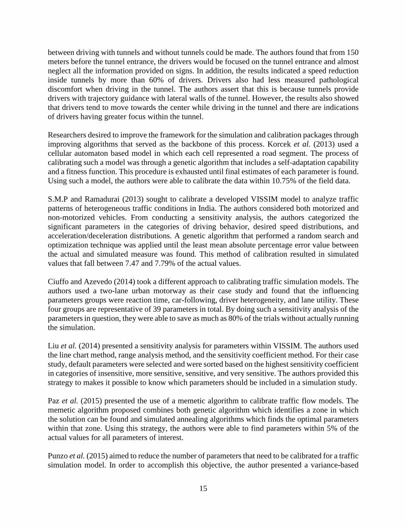
Table 4.2 displays a sample of the data derived from the probe trips. In the probe data, the OBD speed is recorded alongside the GPS speed. Inside the tunnel, the GPS speed cannot operate and the GPS speed inside the tunnel is an interpolation between the speeds before and after the tunnel. The OBD speed has been recorded inside the tunnel and is assumed to be more accurate than the GPS speed. The probe data is appropriate for creating the trajectories of trips inside the HRBT and travel times in congestion hours and non-congestion hours. Figure 4.2 displays sample trajectories which have been created for a few sample probe trips. The vertical axis is distance traveled inside the HRBT and the horizontal axis is time. The bold black horizontal lines represent the tunnel entrance and exit. The shortcoming of the sample probe data and trajectories is that vehicle interactions and driver behavior changes due to such interactions could not be captured since the trajectories of the surrounding vehicles are not observed. Table 4.3 provides a list of the probe recordings from Figure 4.2 that occurred under congestion. TABLE 4.2. Sample Data displayed by the Probe Data Trips

cellphone unixts ts GPS lat GPS long GPS speed OBD speed gpsts samsung SM-G920P 1.43E+12

5/5/2015 12:52 37.01256 -76.3237 65.99503 65.1 52:41.3

samsung SM-G920P 1.43E+12

5/5/2015 12:52 37.01233 -76.3235 66.15907 65.50 52:42.3

samsung SM-G920P 1.43E+12

5/5/2015 12:52 37.0121 -76.3233 65.91936 65.72 52:43.3

samsung SM-G920P 1.43E+12

5/5/2015 12:52 37.01186 -76.3232 65.33737 65.55 52:44.3

samsung SM-G920P 1.43E+12

5/5/2015 12:52 37.01162 -76.3231 64.73515 64.66 52:45.3

samsung SM-G920P 1.43E+12

5/5/2015 12:52 37.01138 -76.323 64.3595 64.19 52:46.3

samsung SM-G920P 1.43E+12

5/5/2015 12:52 37.01113 -76.3229 64.33635 63.86 52:47.3

22

Figure 4.2. The Trajectories of Trips inside the HRBT TABLE 4.3. The Time of Travel of the Congested Trips from the Trajectories in Figure 3

Trip ID Time of Trip Color of Trajectory 247 11/7/2015 1:39 p.m. Yellow 888 11/7/2015 1:42 p.m. Dark Green (right side of chart) 634 7/15/2015 9:52 a.m. Blue (right side of chart) 568 6/15/2015 12:22 p.m. Red

4.3 INRIX SPEED DATA

INRIX is a private company that provides various services pertaining to traffic along roadways. The INRIX utilizes floating cars to provide average speeds in urban and rural roadway segments.. The INRIX data can be used to create heat maps of speeds through and in the upstream of the HRBT. The heat map displays the average traffic speed at different locations at different times for the desired segments. As the speed data collected have different reliability levels, INRIX assigns a confidence score to indicate the reliability of the data. The maximum confidence score is 30, which specifies that the speed data are based on actual speeds from the field. The lowest designated score is 10, which means that the data are estimated from historical values. Figure 4.3 displays a sample speed heat map for one day (07/28/2014) in the eastbound direction of the HRBT.

23

Figure 4.3. The eastbound heat map of the HRBT for 07/28/2014. In Figure 4.3, the color scale is presented at the right with black representing a speed of zero mph, green representing a speed around 70 mph, and white represents a period when data was unavailable. The solid horizontal lines mark ramps and tunnel exits, most of which fall outside the scope of this study. The solid horizontal lines within the boxed section indicate the entrance and exit of the tunnel. The dotted horizontal lines correspond to the boundaries of INRIX Traffic Message Channel (TMC) segments. Congestion occurring prior to the tunnel entrance is classified when speeds in TMC 110N04877 were visually lower than those within TMC 110-04876, and the speed in TMC 110-04876 and downstream are mostly in the range of 50 mph or greater. When the speeds in TMC 110-04876 and downstream are in the 40 mph range or lower, that indicates congestion within the tunnel. The incident data for the studied road segment can be used to determine if speed drops were due to recurrent congestion or incidents.

4.4 WAVETRONIX DATA

Wavetronix is a company that creates tools and detectors for Intelligent Transportation Systems (ITS), including advanced radar sensors, power and communication solutions and data management appliances. Its data recording sensors are located throughout the region, including at the HRBT. The Wavetronix sensors provide speed, occupancy (of the detection area) and volume of vehicles detected on the sensor’s detection area during two minute intervals. There are two sensors for the HRBT. One is located on the bridge upstream the tunnel and one located in the freeway after the

24

HRBT. Figure 4.4 displays the location of Wavetronix sensors relative to the HRBT. The red dots in the map are the locations of the Wavetronix sensors.

Figure 4.4. The Position of the Wavetronix Sensors Table 4.4 below displays the data available from the sensor locations in two minute periods. For this data set, the volume displays the sum of all vehicles passing the detection area within the two-minute period. Occupancy is the percentage of the two-minute period that the detection zone is occupied. When the average speeds are high, occupancy can be lower than one percent (considered 0). The speeds are the average spot speeds. The Wavetronix data does not separate the volume and speed by lane. There is no Wavetronix sensor data available inside the tunnel. TABLE 4.4. The data available from the sensor locations in 2 minute periods.

rec_id station_id Ts volume occupancy Speed (mph) 174219166 0 7/1/2016 0:00 27 2 72 174219167 1 7/1/2016 0:00 16 0 58 174219168 2 7/1/2016 0:00 12 0 56 174219169 3 7/1/2016 0:00 10 0 62 174219170 4 7/1/2016 0:00 18 0 57 174219171 5 7/1/2016 0:00 5 0 60 174219172 6 7/1/2016 0:00 8 0 65 174219173 7 7/1/2016 0:00 18 1 59 174219174 8 7/1/2016 0:00 8 0 56 174219175 9 7/1/2016 0:00 12 0 56 174219176 10 7/1/2016 0:00 6 0 58

25

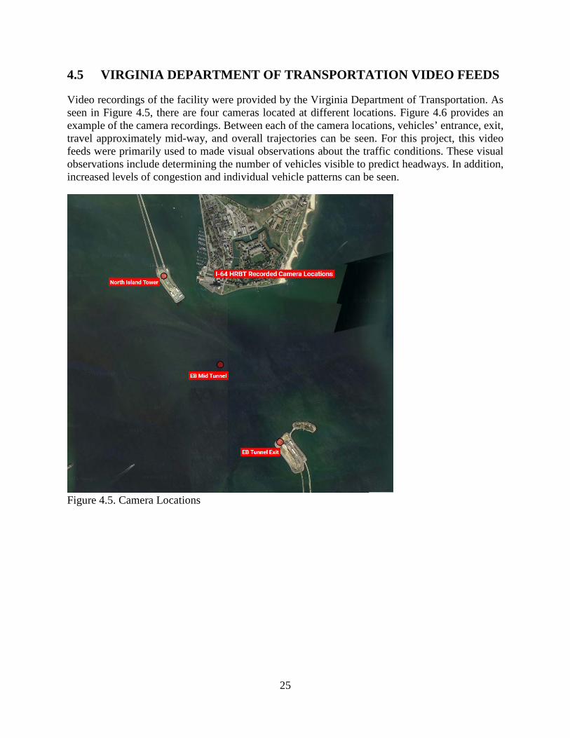
4.5 VIRGINIA DEPARTMENT OF TRANSPORTATION VIDEO FEEDS

Video recordings of the facility were provided by the Virginia Department of Transportation. As seen in Figure 4.5, there are four cameras located at different locations. Figure 4.6 provides an example of the camera recordings. Between each of the camera locations, vehicles’ entrance, exit, travel approximately mid-way, and overall trajectories can be seen. For this project, this video feeds were primarily used to made visual observations about the traffic conditions. These visual observations include determining the number of vehicles visible to predict headways. In addition, increased levels of congestion and individual vehicle patterns can be seen.

Figure 4.5. Camera Locations

26

Figure 4.6. North Island Tower Travel Directions

5.0 VISSIM MICRO SIMULATION MODEL

In order to analyze the traffic flow characteristics through the HRBT tunnel, a microsimulation modes is developed in VISSIM. This model is then calibrated based on the available relevant field data.

5.1 THE VISSIM MODEL FEATURES

One of the major components of every microsimulation programs is its car-following model The microsimulation model deployed in VISSIM primarily features the Wiedemann Car Following Model (Wiedemann, 1974). The Wiedemann car following model was based on the psycho-physical model suggested by Wiedemann in 1974 and has been continuously enhanced since then. Notably, Wiedemann and Reiter further developed the parameters in 1992, including the description of the random numbers in the model (Wiedemann and Reiter, 1992). The Wiedemann car following model utilizes varying thresholds to form the car following regimes. The model includes key parameters line standstill distance, time headway distribution, acceleration, etc. Each are identified as CC0 to CC9 in the driving behavior package besides other relevant car following parameters. These factors can be found under the driving behavior parameters of the VISSIM software package and can be manipulated to yield the desired car

27

following behavior built upon the Wiedemann model. Because of these features VISSIM is selected as a platform for modeling in numerous research projects. In this project, because of the capabilities of the car following model in VISSIM and all of its microsimulation parameters which enable modeling the ground truth with more depth and precision, the HRBT was modeled in VISSIM. The car following parameters were investigated in terms of their relevance for calibration within a tunnel sag curve. Consequently a car following parameter which is considered to model connectivity between vehicles and have a major role in bottleneck formation is examined. In the next part some of the main car following parameters related to this project are introduced.

5.1.1 LOOK AHEAD DISTANCE PARAMETER

The look ahead distance is defined as the minimum and maximum distance that a vehicle can see forward or detect so that it able to react to other vehicles either in front or to the side of it along the same link in the network. In addition to the look ahead distance, vehicles are able to detect the number of preceding vehicles. This parameter is named “Number of Observed Vehicles” in VISSIM. The number of observed vehicles is within the bounds of the maximum look ahead distance. Vehicles can use this information in addition to network objects, such as traffic lights and desired speed change points, to predict other vehicles’ movements and react accordingly. A higher look ahead distance would mean a larger range of vision by the vehicle and thus less abrupt behavior from the vehicles. The default value for this parameter in VISSIM is 870 feet. In the next chapter, a sensitivity analysis of this parameter is presented.

5.1.2 CAR FOLLOWING PARAMETERS

The parameters named under CC0-CC9 in VISSIM are the car following parameters which comprise the main components of the car following in VISSIM. The parameters time headway distribution (CC1), following variation (CC2) and the acceleration profile of vehicles which account for the vehicle kinematics are the significant parameters in the simulation of the HRBT.

5.1.3 TIME HEADWAY DISTRIBUTION

In VISSIM 9, the user can define an empirical or normal distribution for the time headway for any vehicle class in the simulation. The time headway distribution would be selected as the CC1 parameter for any vehicle class within any link. This parameter is an important parameter related to the throughput of the tunnel segment and the congestion within the tunnel section. According to the principles of traffic engineering, a lower desired headway would yield higher throughputs and less travel times in the tunnel section.

28

5.1.4 CAR FOLLOWING VARIATION

The car following parameter called the following variation defines the longitudinal oscillation during a following condition. It restricts the distance difference (longitudinal oscillation) and determines the range of distance additional to the desired safety distance that the following vehicle is within when following another vehicle before intentionally moving closer to the front car. The safety distance in VISSIM can be calculated as; standstill distance (CC0) + [desired time headway (CC1) * Speed]. The following behavior results in distances between desired safety distance and the following variation as shown in Figure 5.1. The default value is 4.0m. According to the VISSIM manual, there would be no oscillation in the distance pursued by the following card if the CC2 value is set to a number close to zero. This would inherently imply an indirect ACC system.

Figure 5.1. Car-Following Behavior

5.1.5 CRAWL SPEEDS

Previous research has shown that vehicles cannot go faster than a certain speed in any uphill grade due to their performance limitations. This final speed is known as the crawl speed and differs between vehicles based on their power to mass ratio and kinematic capabilities. The crawl speeds are generally used to update acceleration/speed profiles of vehicle classes (in the simulation model) in sag curves. In the HRBT, the uphill section has a grade of 4% and a vehicles average speed in the congestion hours is between 15-30 mph. Thus, vehicles still have the capacity to accelerate and the upgrade does not restrain their speeds in the upgrade section.

6.0 CALIBRATION

The major contributing factor to congestion at the HRBT is the demand being higher than the capacity. Other major factors include incidents, disabled vehicles, and over-height truck turnarounds. However, in addition to these, heterogeneous car following behaviors within the traffic at the tunnel also contribute to congestion. The queue formed can back up to approximately several miles upstream the bridge tunnel. This bottleneck is formed at the tunnel entrance in the morning and evening peak hours.

29

Within the tunnel the major contributor to the bottleneck formation is the vehicles change of driving behavior when entering the tunnel and the different driving characteristics of cars entering the tunnel. As cars enter the tunnel, this diversity in driving behaviors of vehicles may lead to phantom jams and bottleneck formation within the tunnel. The differences is mainly in the desired following time headway of different drivers, slow trucks in lane 1 and certain vehicles excessive acceleration/deceleration in the tunnel section. To have the VISSIM simulation calibrated with the available data sources, relevant VISSIM input parameters of the car following model and vehicle kinematics had to be calibrated so that the outputs of speed and travel times would match the field data. The speeds and headways of the PVR data (right after the tunnel exit and before the bridge as seen in figure 4.1) were selected as the field data which were compared with the simulation outputs. The data extracted from the PVR sensors for calibration include a 75 minute congestion period during which bottlenecks formed within the tunnel. The PVR data had 10% HGVs and 90% cars with a throughput of 1,528 vehicles in lane 1 and 1,965 cars in lane 2 (lane 1 having less due to HGV traffic in lane 1). The throughputs of both lanes were also compared to VISSIM throughputs for verification purposes. From the main VISSIM car following parameters (CC0-CC9), the desired speeds of vehicle classes within and outside the tunnel, the desired time headways (CC1) of every vehicle class within and outside the tunnel, the look ahead distance and the vehicle acceleration profiles were considered for calibration with the PVR data. Other VISSIM following parameters such as standstill distance (CC0), following variation (CC2) were seen as less significant based upon the data available. Figure 6.1 displays the driving behavioral parameters of the Wiedemann 99 which is the default car following in VISSIM.

Figure 6.1. The driving behavioral parameters in VISSIM.

30

The acceleration profiles of cars and HGVs can be determined from the maximum and desired acceleration curves within VISSIM so that they would have the same behavior as the crawl speeds mentioned in the previous chapter. In the case study of the HRBT, the length of the upgrade segment (being less than what is needed for vehicles to reach crawl speeds) plus the slow speeds (less than 40 mph) within the congestion undermined the significance of that parameter and therefore the default curves were used. With attention to the car following parameters (in Figure 6.1.) and the assumed significance of each parameter, for calibrating the car following model with the PVR data, the time headways, CC1, look ahead distance and the desired speeds were manipulated. The desired speeds of cars ranging from an empirical distribution with [55mph-70mph] outside the tunnel reduces to an empirical distribution of [40mph-60mph] inside the tunnel. The desired speeds distribution is once more modified to an empirical distribution of [38mph – 70 mph] at the start of the upgrade section in the HRBT so that our simulation results at the data collection points would be matching the PVR speed distribution. The look ahead distance is also reduced from 250ft to 150ft at the start of the tunnel segment. The desired time headway distribution of vehicles remains the same in the tunnel from the upstream freeway until the uphill section when it changes from [0.5s - 2s] to [1s - 4s]. The first two changes were made to replicate usual driver behavior change within the tunnel. The latter change was to have the vehicles in the upgrade section in accordance to the headways obtained from the PVR, considering the required distance for vehicles to adapt to that behavior. The travel times of probe trips recorded in congested conditions within HRBT were also considered and compared with the travel times obtained from VISSIM simulations. Figure 6.2 presents a comparison between the simulation outputs and PVR for speed and headway distribution within lane 2 of the HRBT. Their comparison displays the same trend followed by vehicles at the data collection point. There were limited number of travel times recorded from probe trips in congestion, which those probe trips had a travel time of approximately 250 seconds within the tunnel segment of the HRBT. After making the necessary adjustments to the car following parameters in VISSIM, the simulation was calibrated to produce results as close as possible to the field conditions. Figure 6.2 shows that headway and speed distributions from VISSIM are matching relatively well with the field data.

31

Figure 6.2. The calibrated results of simulation compared with the PVR data for lane 2

7.0 IMPACTS OF CONNECTED VEHICLES

In this section, how connected vehicles can impact the traffic performance will be investigated. More specifically, CVs in the traffic stream will be assumed to have additional information (that is not available to non-CVs) that would impact the driver behavior. By influencing the driving behavior of CVs the overall system performance is expected to improve. This section shows how this could be done by first providing a longer look-ahead distance; and by employing a variable speed limit strategy in the upstream of the sag curve.

32

7.1 CONNECTED VEHICLES IN MIXED TRAFFIC

The Connected Vehicles (CVs) will be gradually entering the traffic as their technologies develop and they become more commercialized. It is anticipated that during the next 2 decades they will steadily take over half of the traffic. The exact capabilities of the vehicles and communications between them is still not clear as they are in the developing phase but their approximate driving behaviors have been clarified in numerous studies. As it will take many years for all vehicles in the traffic to have connectivity, the traffic behavior of mixed traffic of connected and non-connected vehicles is current research topic. With the advent of inter-vehicle communications (V2V) and communications between vehicles and the infrastructure (V2I), higher safety levels and higher capacity (in urban and rural roads) are expected. In the next section, an analysis of downstream visibility and its effect on the traffic performance is carried out.

7.1.1 Analysis of Look Ahead Distance

In this section, the impacts of increased look-ahead distance are investigated through microsimulation. The VISSIM model developed and calibrated (in the previous section) for the current congested operating conditions of the HRBT is used for simulating the effect of Look Ahead Distance (LAD). This was due to the fact that the lack of downstream observability was regarded as a key factor in shockwave and phantom jam generation within a tunnel which led to bottleneck formations and a lower throughput of that tunnel. The LAD in VISSIM is a significant parameter in car-following behavior as it is related to shockwave creation and propagation. A higher look-ahead distance is defined for new vehicle class created within VISSIM. Vehicles in this class are considered to be connected vehicles that can receive information about downstream vehicles and conditions. In the simulations, the percentage of CVs in the traffic stream is varied to understand the impacts on the tunnel throughput and travel times. Table 7.1 depicts the different trials of simulation. In the base traffic, there are no CVs. In scenarios 1 to 4, there are different LADs for the CVs ranging from 300 feet to 750 feet. The base scenario’s LAD replicates regular manual cars’ observability of the preceding vehicles when traveling through the tunnel section. The levels of LAD within the simulation scenarios depict varying levels of observability of CVs within the tunnel section. The distances selected for the LADs in the simulation scenarios are multiplies of 150 feet, a non-equipped car’s observability within the tunnel. The maximum range of 750 feet is associated with sensor/radar coverage forecasted for I2V communications (Laquai, 2011). From a traffic flow perspective, higher LADs are expected to yield more harmonious and homogenous traffic which should lead to an increase in the tunnel throughput and reduction in the travel times. The simulation results for each of the scenarios are summarized in Table 7.2. Average and median travel times from both lanes were first calculated for one hour in simulation time when the traffic was experiencing congestion. Congestion in the simulation is defined when speeds in the bridge

33

tunnel are below 40 mph and bottlenecks have formed either before or inside the tunnel. The throughputs for each lane of the freeway segment are also displayed for the same hour. TABLE 7.1. Simulated Scenarios

Simulation Scenario Look-ahead distance (ft)

Percentage of CVs

Base condition 150 0 Scenario 1 300 20, 50, 80, 100 Scenario 2 450 20, 50, 80, 100 Scenario 3 600 20, 50, 80, 100 Scenario 4 750 20, 50, 80, 100

TABLE 7.2. Simulation results

Simulation Scenarios (look-ahead distance)

Percentage of Probe Vehicles (%)

Average Travel Time (s)

Median Travel Time (s)

Throughput Lane 1 (vph)

Throughput Lane 2 (vph)

Base 0 307 329 1250 1490 20 298 311 1338 1564 50 219 307 1315 1560 80 283 305 1327 1609 100 284 289 1675 1683 20 307 317 1360 1575 50 297 308 1310 1580 80 278 301 1348 1628 100 280 285 1670 1672 20 305 315 1365 1555 50 300 312 1314 1575 80 286 302 1308 1613 100 273 276 1692 1705 20 296 310 1377 1570 50 297 309 1337 1583 80 280 295 1332 1607 100 272 276 1713 1694

34

As the percentage of the CVs (which have higher LAD) increases in the traffic for each scenario, the travel times through the tunnel decline. The throughputs have an increasing trend in the left lane that carries only passenger cars. For the right lane with mixed traffic of vehicles and HGVs, the throughputs do not experience any significant improvements until the traffic stream is solely CVs at 100% market penetration, which illustrates the effect of HGVs on that lane. When there are only CVs, there exists a rapid increase of the throughput on lane 1. For example, in scenario 1 with 100% CVs, the lane throughputs have increased by 34% and 13% for lanes 1 and 2 respectively. With a higher look-ahead distance for the CVs, the travel times are shown to be reduced by 14% and the tunnel throughput increased by 20%. With the maximum LAD for CVs, the throughputs become 14% higher in lane 2 and 37% higher in lane 1, the lane with mixed traffic. This shows a positive relationship between the vehicle observability and the throughput of the tunnel section. However, the marginal increase in throughput diminishes as the LAD is increasing. The average and median travel times gradually decrease with higher percentages of probe vehicles and with higher LADs. On the other hand, the increase of the percentage of probe vehicles leads to the average and median of the travel times becoming closer in value. This implies that the traffic is becoming more homogenous and therefore creates smoother driving behaviors. As seen in Table 2, not all values follow the general trends as described. This could be attributed to the stochastic elements in the microsimulation model, such as vehicle generation and the driving behavior processes. From the overall results obtained, it can be concluded that increasing LADs will lead to reduced travel times and increased throughput for the tunnel.

7.2 VARIABLE SPEED CONTROL IN A SAG CURVE

Implementing a control system in the upstream section of a traffic segment as an approach to optimize the traffic flow has been pursued by researchers. A few examples of this method were discussed in Section 2. In the following section of this report, a control strategy with the use of a modified version of the IDM model is tested for its results in yielding better travel times and less delays through a sag curve.

7.2.1 Variable Speed Limit Control Strategy for Sag Curves

Longitudinal Driving Behavior- Intelligent Driver Model The Intelligent Driver Model (IDM) is a time-continuous car-following model for the simulation of freeway and urban traffic. It was developed by Treiber, Hennecke and Helbing in 2000 to improve upon results provided with other "intelligent" driver models such as Gipps' model, which lose realistic properties in the deterministic limit (Treiber et al., 2000). The model is based on the following equation.

𝑣𝑣𝑣(𝑡𝑡) = 𝑓𝑓𝑟𝑟(𝑡𝑡)

35

where v̇(t) is the optimal velocity at time, t fr(t) is the function of velocity

𝑓𝑓𝑟𝑟(𝑡𝑡) = 𝛼𝛼 ∗ min �1 − �𝑣𝑣(𝑡𝑡)𝑣𝑣𝑑𝑑𝑑𝑑𝑑𝑑(𝑡𝑡)

�4

, 1 − �𝑠𝑠∗(𝑡𝑡)

𝑠𝑠(𝑡𝑡) − 1�2

�

where α is the specific vehicle parameter vdes(t) is the desired velocity s*(t) = desired minimum gap s(t) = the actual gap

𝑠𝑠∗(𝑡𝑡) = 𝑠𝑠0 + 𝑣𝑣(𝑡𝑡) ∗ 𝜏𝜏(𝑡𝑡) + 𝑣𝑣(𝑡𝑡) ∗ 𝛥𝛥𝑣𝑣(𝑡𝑡)

2 ∗ √𝑎𝑎𝑎𝑎

where s0 is the jam distance τ(t) is vehicle relaxation times a is the maximum acceleration b is the desired deceleration

𝜏𝜏(𝑡𝑡) = �𝜏𝜏0, 𝑣𝑣(𝑡𝑡) ≥ 𝑣𝑣𝑐𝑐𝑟𝑟𝑐𝑐𝑐𝑐

𝛾𝛾 ∗ 𝜏𝜏0, 𝑣𝑣(𝑡𝑡) < 𝑣𝑣𝑐𝑐𝑟𝑟𝑐𝑐𝑐𝑐

where vcrit is the critical velocity γ is In summary, this model determines an optimal velocity based on individual vehicle properties and spacing within the network. In this section of the study, the model Goni-Ros et al. (2014) proposed for sag curves is used. This model accounts for the influence of vertical curves on vehicle acceleration. It calculates acceleration from the summation of two terms as presented in Equation 1.

)()()(' tfgtfrt +=υ (1)

The first term uses speed, relative speed, and spacing to the vehicle ahead to calculate acceleration for the following car. This is a modified version of the IDM.

∆−

−×=

24

)())(),((

1,)(1min)(ts

ttstatfr des

des

υυυυ

(2)

In Equation 2, dess is the desired spacing which is computed using Equation 3. The main influencing factor is the safe gap to the lead vehicle.

36

battttstVtVsdes .2)().())(().())(),(( 0

υυυτυ ∆++=∆

(3)

The 𝑣𝑣𝑑𝑑𝑑𝑑𝑑𝑑 is the desired speed; a is the maximum acceleration, 𝑎𝑎 is the maximum comfortable deceleration, 𝑠𝑠0is the gap at the standstill situation, and τ is the safe time headway as a function of speed. Based on the traffic state, the safe time headway (τ ) changes as shown in Equation 4.

<≥

=critf

critf

tt

tυυτγυυτ

υτ)(.)(

))((

(4)

The second term ( )(tfg ) in Equation 1 captures the influence of gradient on vehicle acceleration. This influence is equal to the difference between the gradient at the position of the vehicle (

))(( txG ) and the compensated gradient by the driver at the time (𝐺𝐺𝑐𝑐(𝑡𝑡)) multiplied by gravity acceleration. This is shown in Equation 5.

))())((.()( tGtxGgtfg c−−=

(5)

Ros et al. (2014) assumed that drivers would compensate linearly for any increase in freeway gradient with maximum gradient compensation rate defined by parameter c.

−+−+≤

=otherwisettctG

ttctGtxGtxGtG

cc

ccc )()(

)()())(())(()(

(6)

Where:

[ ]))(()(|max txGtGtt cc == (7)

If the increase in grade over time is lower than c, then 𝐺𝐺𝑐𝑐(𝑡𝑡) is equal to 𝐺𝐺𝑥𝑥(𝑡𝑡) and 𝑓𝑓𝑓𝑓(𝑡𝑡) is zero. Hence, the acceleration of vehicle is not affected and the driver fully compensates for the gradient. Control strategy The objective of the control strategy is to eliminate congestion in sags and improve the performance of highways in hilly regions. For networks not influenced by other control measures, minimizing the total time that vehicles spend in the system is equivalent to maximizing the exit flow (Papageorgiou, 2003). As mentioned previously, under uncongested traffic conditions, flow or throughput is higher than that under congested conditions. The capacity of the freeway on a sag

section ( sagq ) is less than other sections ( Capacityq ). Therefore, the network’s exit flow is limited by the capacity of the sag bottleneck.

Capacitysagexit qqq <≈

(8)

37

One way to maximize the exit flow is to prevent traffic from becoming congested at the bottleneck. Keeping traffic state uncongested at the bottleneck is possible if the inflow of the sag gets regulated using a controlled section at the upstream. The inflow of sag is approximately equal to the outflow of the control section, and per the fundamental relation between speed and flow, changing speed on control section changes the inflow of the sag. By dynamically modifying the speed at control section, it is possible to keep the inflow to the bottleneck slightly below its free flow capacity. This will increase the time-weighted sum of exit flow. When the demand in the upstream is large enough, the congestion would not be prevented completely. As a result, the control section and upstream would become congested instead of the sag curve, but the outflow from the controlled part will be higher than the queue discharge capacity of the sag. The controller which calculates speed limit for the control section is inspired from the ramp-metering control algorithm called ALINEA and proposed by Papageorgiou et al. (2003). This algorithm is based on the basics of a proportional feedback control law. It calculates the variable

speed limit based on Equation 9. The target density ( etT argρ ) is slightly lower than the critical

density of fundamental diagram, and real-time density ( bρ ) is the estimated/measured density at the sag curve calculated every 𝑇𝑇𝑐𝑐 seconds. The algorithm would change the speed limit as a proportion (κ ) of the difference between target and measured density every time that a new density is calculated.

))1(()( argarglim −−×+= tt betTetTit ρρκυυ (9)

As evident from Equation 9, in high demand conditions, the controller would keep the density at bottleneck close to target density to prevent breakdown. Whenever demand decreases, the measured density would be significantly less than target density which leads the controller to impose a higher speed limit and in contrary if demand increases measured density would be substantially more than target density which leads the controller to enforce a lower speed limit. The controller always uses previously estimated density so that drivers would have enough time to cover the distance between the control section and the bottleneck. Two roadside units, shown in Figure 1, are needed for system operation. The roadside unit A is connected to a typical loop detector that measures occupancy and estimates density at the bottleneck every 𝑇𝑇𝑐𝑐 seconds. This information is then transmitted to roadside unit B in the upstream. Based on Equation 9, the roadside unit B would update speed limit every 𝑇𝑇𝑐𝑐 seconds and broadcast it to the connected vehicles (CVs) when they arrive at the control section every second. The geometry of the network and traffic flow parameters are explained next.

38

Figure 7.1. Geometry of the sag curve Simulation setup The simulation model comprises a one-lane freeway with a sag in the middle. The length of the facility is 12 km. The road starts with constant-gradient downhill section followed by a vertical sag curve, and at the end, a constant-gradient uphill section (see Figure 7.1.). The downhill section has a constant gradient equal to -0.5 percent and the uphill section has a constant slope equal to 2.5 percent. At the vertical sag, the slope increases linearly from -0.5 to +2.5 percent, and the length of the vertical curve is 400 m between x = 10.7 km and x = 11.3 km. The downhill section is long enough to make sure queue would not reach the entry point of the simulation. The speed limit is 120 km/h. Characteristics of vehicles and drivers, as defined by the IDM model, are assumed to be homogeneous to prevent the emergence of other types of bottlenecks in the simulation as shown in Table 7.3. TABLE 7.3. Characteristics of the car-following model

)( hkm

desυ )( 2s

ma

)( 2smb

)(sτ )(0 ms )( h

kmcritυ

)(−γ )( 1−sc )(st∆

120 1.45 2.1 1.2 3 65 1.15 0.0001 0.5 The distribution of demand over time is illustrated in Figure 7.2. The first 10 minutes is a transition from zero to 2400 veh/h, a capacity higher than the bottleneck capacity. The demand stays at 2400 veh/h for 30 minutes then transitions back to zero across 10 minutes. Beyond this, the demand remains zero until all vehicles have exited the facility.

39

Figure 7.1. Demand profile over time The control section in Figure 1 is 1.0 km long. In this section, only connected vehicles would be informed of the calculated speed limit. Notably, it is assumed that all CVs would comply completely. The control section is between x = 9.3 km and x = 10.3 km. The downstream end of the controlled section is 0.4 km away from the beginning of the transition section. As soon as connected vehicles leave the control section, their speed will revert to the default 120 km/h to make sure the vehicles traverse the uphill with the maximum speed possible. In other words, the desired speed of CVs is only varied while they are within the control section. With the given parameters above, a microsimulation model was created in MATLAB. In Figure 7.3, a heatmap along with sample vehicle trajectories are shown (middle chart) for the base case, i.e. when no control strategy is implemented. At the very beginning of the simulation, the effect of the uphill is not significant enough to cause a breakdown at the bottleneck. After a while, a shockwave starts to propagate backward starting at the bottleneck with constant speed. Since the breakdown is due to the geometry of the road, this shockwave continues to propagate until in-flow decreases.

40

Figure 7.3. Input demand and exit flows (top left), density measured by loop detector (bottom left), heat-map with sample trajectories (middle), average vehicle speeds in the control section (top right), and number of vehicles in the system (bottom right) without a VSL control system Four other charts are included to provide additional performance measures for analysis in Figure 7.3. At the top left, the input demand over time (green line), as well as exit flow rates, are depicted for the base case (red line). A hypothetical scenario (black line) where the uphill has no influence whatsoever on the traffic flow is also shown. This last scenario is included as a reference to show the maximum possible system performance if the effects of sag are eliminated. This phenomenon could perhaps be achieved through automated driving, but this is left for future research. The second chart, density versus time plot at the lower left, shows the measured density by the loop detector at the uphill (see Figure 7.1). The chart on the top right shows the observed speed (red line) at the control section as well as the imposed VSL. The last chart at the bottom right reports the total number of vehicles in the system, i.e. for the entire corridor, over time for the base case without a VSL system (red line) as well as for the hypothetical scenario (black line). These charts are reproduced to summarize the effects of VSL under various CV market penetrations as presented later in the report. A meta-heuristic for the optimal control parameter values The VSL control strategy described by Equation 9 requires three key parameters to achieve optimal performance. Here, the total delay in the system is used as the objective function. The delay for a vehicle is computed in reference to the hypothetical scenario mentioned above, where the sag curve is assumed to have no influence on the traffic flow. For the simulated demand, vehicles travel through the corridor at free flow speeds. For a given scenario, the total delay is the sum of the individual vehicle delays. For example, when there is no VSL control system, the system performs as shown in Figure 7.3. This total delay (TD) is then taken as a reference and compared to the total delay for the VSL control strategies. Consequently, the objective function is defined as shown in Equation 10.

NoControl

ControlledNoControl

TDTDTD

unctionObjectiveF−

=

(10)

Optimizing three parameter values is the objective: the gain ( κ ), the period for sampling occupancy at bottleneck (𝑇𝑇𝑐𝑐), and the target speed (𝑉𝑉𝑐𝑐𝑡𝑡𝑟𝑟𝑡𝑡𝑑𝑑𝑐𝑐). Since a mathematical formulation for this optimization problem does not exist, the authors used a meta-heuristic. The hybrid particle swarm optimization genetic algorithm (HPSOGA) proposed by Duan et al. (2013) was used. The particle swarm optimization (PSO) simulates the behavior of a swarm of particles moving to a potential well with an analogy to the flocking of birds or fish schooling. Random parameters for all particles are generated and the objective function for each particle is calculated. For this problem, a good position for a particle corresponds to a lower value of the objective function. Based on equations of the algorithm, the particles move in the search space of the problem. The algorithm has two basic equations shown below. These equations update the positions of the particles in every iteration.

)1()()1( ++=+ ttxtx iii υ (11)

))()(.())()(.()(.)1( 21 txtxctxtxctt iGlobalBestii

LocalBestiii −+−+=+ υωυ

(12)

41

Each particle moves in accordance with Equation 11. The velocity 𝑣𝑣𝐼𝐼𝑐𝑐+1 is computed from the best memory of each particle (𝑥𝑥𝐼𝐼𝐿𝐿𝐿𝐿𝑐𝑐𝑡𝑡𝐿𝐿𝐿𝐿𝑑𝑑𝑑𝑑𝑐𝑐 (𝑡𝑡)) over previous generations up to step t and from the swarm global best (𝑥𝑥𝐼𝐼𝐺𝐺𝐿𝐿𝐿𝐿𝑐𝑐𝑡𝑡𝐿𝐿𝐿𝐿𝑑𝑑𝑑𝑑𝑐𝑐 (𝑡𝑡)). The first term in Equation 12 is called inertia, and it is a portion of the previous velocity of the particle. The ω factor is called the inertia weight, and it is a constant between 0.4 and 0.9 (in this study it is considered 0.9). The c1 factor is a constant called the cognitive or local weight. The term (𝑥𝑥𝐼𝐼𝐿𝐿𝐿𝐿𝑐𝑐𝑡𝑡𝐿𝐿𝐿𝐿𝑑𝑑𝑑𝑑𝑐𝑐 (𝑡𝑡) − 𝑥𝑥𝑐𝑐(𝑡𝑡) ) means the distance between the position of the best personal experience and the present position of the particle. The third term is called global movement. The c2 factor is a constant called the social or global weight. The (𝑥𝑥𝐼𝐼𝐿𝐿𝐿𝐿𝑐𝑐𝑡𝑡𝐿𝐿𝐿𝐿𝑑𝑑𝑑𝑑𝑐𝑐 (𝑡𝑡) − 𝑥𝑥𝑐𝑐(𝑡𝑡)) means the distance between the position of the best collective experience and the present position of the particle. Once the new velocity has been determined, it is used to compute the new particle position from Equation 11. The solution from the PSO becomes the initial population of the genetic algorithm. The genetic algorithm (GA) has three stages: Stage 1: Creating an initial population; Stage 2: Evaluating an objective function; and Stage 3: Producing a new population. GA operators manipulate each member. The first operator is a crossover which selects two members of the population as parents and produces two offspring by swapping elements of the parents. Participating in a crossover depends on the value of each member’s objective function which means members with higher values participate in crossovers more often. The second operator is a mutation operator. It is used to increase the space explored. The mutation rate is low. In the end, a new population is selected from the output of these two operators and the process continues. If identical solutions are obtained, the best solution is assumed to be determined. The three control parameters were optimized using HPSOGA algorithm with a population size of 50 and a maximum iteration number of 100. The optimal parameters found by the algorithm are presented in Table 7.4. TABLE 7.4. Optimum parameters for the VSL control strategy

Optimal parameters

)(arg hkm

etTυ κ )(sTc

95 4.68 50 The resulting system performance is shown in Figure 7.4. The market penetration rate is 100%. The VSL reduced the total delay by 49% compared to the no control scenario. The shockwave is moved upstream of the control section. The density at the bottleneck stays below 25 veh/km at the onset of congestion and the system is able to reach a steady-state density and approximately constant VSLs after 35 minutes. In the top-right chart, it is clear that vehicles adhere to the imposed VSLs since their average speeds follow the VSLs. In the bottom-right graph, the blue-line approximately splits the area between black and red lines into two equal pieces, visually demonstrating that the total delay is reduced by about 50%. It should also be noted that the queue dissipation time is shorter under the VSL control system.

42

Figure 7.4. Input demand and exit flows (top left), density measured by loop detector (bottom left), heat-map with sample trajectories (middle), average vehicle speeds in the control section (top right), and number of vehicles in the system (bottom right) with a VSL control system at 100% CVs market penetration (delays are 49% lower than no control) Sensitivity to the market penetration rate In this section, the market penetration level of the CVs is varied to understand the impacts on system performance. As arrivals of connected vehicles are assumed to be random, each market penetration level has been simulated 50 times to account for the variability. The results regarding reductions in total delays are presented as notched boxplots in Figure 7.5. First, as a percentage of VCs increases, the average improvement also increase but at a decreasing rate. Beyond a relatively small value of 15% market penetration, the average improvements are not substantially different from the maximum possible value of 49%. Second, there is substantial variation in the low market penetration rates, which rapidly diminishes with increasing CVs in the traffic stream.

43

Figure 7.5. Notched boxplot of sensitivity analysis Additional analyses are done to understand reasons behind the significant variations in the low market penetration levels. As it is shown in Figure 7.5, the highest variation is at the 5% penetration level which has improvements as high as 45%, or worse than the no control scenario. These two extreme cases are presented in Figure 7.6 and Figure 7.7 respectively. Each vertical red line added to the density diagrams (bottom left) indicates the exact time that a CV enters the control section. It is noticeable that the magnitude of improvement is correlated with the distribution of the arrivals of connected vehicles over time. Whenever there is a large gap between the arrival of connected vehicles, density tends to rise with a delay.

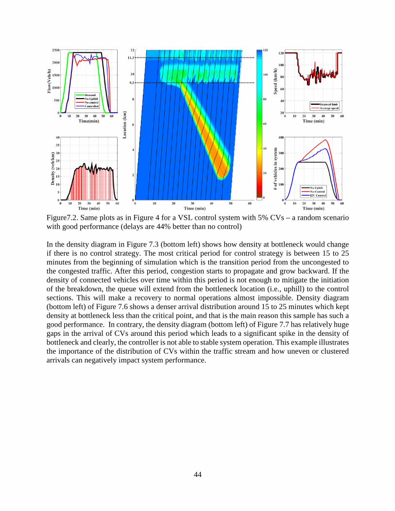
44

Figure7.2. Same plots as in Figure 4 for a VSL control system with 5% CVs – a random scenario with good performance (delays are 44% better than no control) In the density diagram in Figure 7.3 (bottom left) shows how density at bottleneck would change if there is no control strategy. The most critical period for control strategy is between 15 to 25 minutes from the beginning of simulation which is the transition period from the uncongested to the congested traffic. After this period, congestion starts to propagate and grow backward. If the density of connected vehicles over time within this period is not enough to mitigate the initiation of the breakdown, the queue will extend from the bottleneck location (i.e., uphill) to the control sections. This will make a recovery to normal operations almost impossible. Density diagram (bottom left) of Figure 7.6 shows a denser arrival distribution around 15 to 25 minutes which kept density at bottleneck less than the critical point, and that is the main reason this sample has such a good performance. In contrary, the density diagram (bottom left) of Figure 7.7 has relatively huge gaps in the arrival of CVs around this period which leads to a significant spike in the density of bottleneck and clearly, the controller is not able to stable system operation. This example illustrates the importance of the distribution of CVs within the traffic stream and how uneven or clustered arrivals can negatively impact system performance.

45

Figure 3.7. Same plots as in Figure 4 for a VSL control system with 5% CVs – a random scenario with bad performance (delays are 2% worse than no control)

8.0 CONCLUSION AND FUTURE WORKS

The HRBT corridor along the Interstate 64 was modeled as a case study to investigate bottleneck formation within a freeway and how connected vehicles can improve the traffic performance by minimizing the impacts of bottlenecks and congestion. From the investigation of the car following in VISSIM, the look ahead distance parameter, which is downstream observability, was tested. The look ahead distance was tested for a class of cars as probe cars who benefited from a higher downstream observability. The connected vehicles receive information about downstream conditions to better inform the driver about upcoming perturbations in the traffic stream. The results of the tests were improved throughputs for the tunnel section and lower travel times within the congestion.

Furthermore a sag curve was modeled to understand the capability of a variable speed limit control algorithm and connectivity between probe vehicles in mitigating the delay and improving the throughput in a congested sag curve. The VSL control strategy was developed to regulate the speed of CVs in the upstream of the bottleneck on a sag curve and prevent traffic from breaking down by using a proportional feedback control law. The results show that with optimal parameters for control strategy, nearly half of the delay caused by the uphill can be eliminated. Besides that the rate of the probe vehicles had a significant impact on improving the traffic performance. The model displayed how a VSL strategy integrated with CVs can have a considerable role in minimizing the negative aspects of congestions and prevent bottleneck formations. However, the control strategy

46

is sensitive to the arrival times of CVs. If arrival times of CVs are not dense enough at the beginning of high demand, the performance of the system could drop considerably.

There are numerous possibilities for extending this research. It is clear that connected and automated vehicles will play a transformative role in shaping the transportation systems. New car following models which take into account connectivity between vehicles and automated and driver assist features such as Cooperative Adaptive Cruise Control and Adaptive Cruise Control can also be developed and investigated. These models will be important for designing new control strategies for preventing bottlenecks within a tunnel sag curve.

47

REFERENCES

1. Anuar, K., Habtemichael, F., Cetin, M. “Estimating Traffic Flow Rate on Freeways from Probe Vehicle Data and Fundamental Diagram.” 2015 IEEE 18th International Conference on Intelligent Transportation Systems. 2015.

2. Argote-Cabañero, J., Christofa, E., Skabardonis, A. “Connected vehicle penetration rate for estimation of arterial measures of effectiveness.” Transportation Research: Part C, Vol. 60, pp. 298-312. 2015.

3. Bachmann, C., Abdulhai, B., Roorda, M.J., Moshiri, B. “A comparative assessment of multi-sensor data fusion data techniques for freeway traffic speed estimation using microsimulation modeling.” Transportation Research: Part C, Vol. 26, pp. 33-48. 2012.

4. Badillo B., Rakha, H., Rioux, T., Abrams, M. “Queue Length Estimation using Conventional Vehicle Detector and Probe Vehicle Data.” 2012 15th International IEEE Conference on Intelligent Transportation Systems. Anchorage, Alaska, USA. Sept. 16-19, 2012.

5. Bagheri, E., Mehran, B., Hellinga, B. “Real-Time Estimation of Saturation Flow Rates for Dynamic Traffic Signal Control Using Connected-Vehicle Data.” Transportation Research Record: Journal of the Transportation Research Board, No. 2487, pp. 69-77. 2015.

6. Bekiaris-Liberis, Bikolaos, Roncoli, C., Papageorgiou, M. “Highway Traffic State Estimation with Mixed Connected and Conventional Using Speed Measurements.” 2015 IEEE Internation Conference on Intelligent Transportation Systems. Anchorage, Alaska, USA. Sept. 16-19. 2015.

7. Ben-Akiva, M., Cuneo, D., Hasan, M., Jha, M., Yang, Q. “Evaluation of freeway control using a microscopic simulation laboratory.” Transportation Research: Part C, Vol. 11, pp. 29-50. 2003.

8. Calvi, A., De Blasiis, M.R., Guattari, C. “An Empirical Study of the Effects of Road Tunnel on Driving Performance.” SIIV- 5th International Congress – Sustainability of Road Infrastructures. Procedia-Social and Behavioral Sciences, Vol. 53, pp. 1100-1110, 2012.

9. Cascetta, E., Punzo, V., Montanino, M. “Empiricial Analysis of Effects of Automated Section Speed Enforcement System on Traffic Flow at Freeway Bottlenecks.” Transportation Research Record, Vol. 2260, pp. 83-93. 2011.

10. Cetin, M., F. G. Habtemicheal and K. A. Anuar. “Investigation of Sources of Congestion at the Hampton Roads Bridge Tunnel (HRBT).” Norfolk, 2014.

11. Chamberlayne, E., Rakha, H., Bish, D. “Modeling the capacity drop phenomenon at freeway bottlenecks using the INTEGRATION software.” Transportation Letters, Vol. 4:4, pp. 227-242. 2013.

48

12. Chen, C., Kianfar, J., Edara, P. “New Snapshot Generation Protocol for Travel Time Estimation in a Connected Vehicle Environment.” Transportation Research Record: Journal of the Transportation Research Board, No. 2424, Washington D.C., pp. 1-10. 2014.

13. Chiappone, Sandro, Orazio Giuffre, Anna Granà, Raddaele Mauro, and Antonio Sferlazza. “Traffic Simulation models calibration using speed-density relationship: An automated procedure based on genetic algorithm.” Expert Systems with Applications, Vol. 44, pp. 147-155. 2016.

14. Chung, Koohong, Jittichai Rudjanakanoknad, and Michael Cassidy. “Relation between traffic density and capacity drop at three freeway bottlenecks.” Transportation Research Part B, Vol. 41, pp. 82-95. 2007.

15. Cieffo, Biagio and Carlos Lina Azevedo. “A Sensitivity-Analysis-Based Approach for the Calibration of Traffic Simulation Models.” IEEE Transactions on Intelligent Transportation Systems,Vol. 15, No. 3, pp. 1298-1309. 2014.

16. Coifman, B., “Empirical flow-density and speed-spacing relationship: Evidence of vehicle length dependency.” Transportation Research Part B, Vol. 78, pp. 54-65. 2015.

17. Daganzo, C. F. “On the macroscopic stability of freeway traffic.” Transportation Research Part B, Vol. 45, pp. 782-788. 2011.

18. Daganzo, C. F. and Laval, J.A. “On the numerical treatments of moving bottlenecks.” Transportation Research Part B, Vol. 39, pp. 31-46. 2005.

19. Dinh, Tu-Uyen J, Billot, Pillet, and Nour-Eddin El Fauozi. “Real-Time Queue-End Detection on Freeways with Floating Car Data.” Transportation Research Record, No. 2470, pp. 46-56. 2014.

20. Dowling, R., Cohen, M., Skabardonis, Elias, A. “Methodology to Evaluate Active Transportation and Demand Management Strategies.” 6th International Symposium on Highway Capacity and Quality of Service, Stockholm, Sweden, June 28-July 1, 2011.

21. Duan, H., Luo, Q., Ma, G. “Hybrid Particle Swarm Optimization and Genetic Algorithm for Multi-UAV Formation Reconfiguration.” IEEE Computational Intelligence Magazine, Vol. 8, Issue: 3. 2013.

22. Englund, C., Chen, L., Voronov. “Cooperative speed harmonization for efficient road utilization.” 7th International Workshop on Communication Technologies for Vehicles. 2014.

23. Gazis, D.C., Herman, R. “The moving and ‘phantom’ bottlenecks.” Transportation Science, Vol. 26, pp. 223-229. 1992.

24. Gomes, G., May, A., Horowitz, R. “Congested Freeway Microsimulation Model Using VISSIM.” Transportation Research Record, No. 1876, pp. 71-81. 2004.

49

25. Goodall, N., Park, B., Smith, B. “Microscopic Estimation of Arterial Vehicle Positions in a Low-Penetration-Rate Connected Vehicle Environment.” Journal of Transportation Engineering, Vol. 140(10). 2014.

26. Google Maps. https://www.google.com/maps/.

27. Grumert, E., and Tapani, A. “Impacts of a Cooperative Variable Speed Limit System.” 8th International Conference on Traffic and Transportation Studies. Changsha, China, August 1-3, 2012.

28. Guo Chun, Wang Mingnian and Yang Lu. “Intelligent Traffic Safety Control Technology of Highway Adjoining Tunnel and Tunnel Group.” ICTE, pp. 1957-1962. 2013.

29. He, Sheng-Xue. “Will a higher free-flow speed lead us to a less congested freeway?” Transportation Research Part A, Vol. 85, pp. 17-38. 2016.

30. Herkt, S. “A traffic control system for an access tamp to an urban tunnel.” Golden River Traffic. 1990.

31. Hongke, Xu, Chuai Jinhua, Chen Dashan and Xu Na. “Simulation of Highway Tunnel Traffic Control and Guidance.” The Eighth International Conference on Electronic Measurement and Instruments. 2007.

32. Jenelius, E., Koutsopoulos, H. N. “Probe vehicle data sampled by time or space: Consistent travel time allocation and estimation.” Transportation Research: Part B, Vol. 71, pp. 120-137. 2015.

33. Jha, M.,, Cuneo, A., Ben-Akiva, M. “Evaluation of Freeway Lane Control for Incident Management.” Journal of Transportation Engineering, Vol. 125, No. 6, pp. 495-501. 1999.

34. Jin, Sheng, Dianhai Wang and Dongfang Ma. “Empirical Analysis of Traffic Bottleneck at Beijing Expressways.” Mathematical Problems in Engineering, 2013.

35. Jin, Wen-Long and Huiya Jin. “Analysis and design of variable speed limit control system at a freeway lane-drop bottleneck: A switched systems approach.” 53rd IEEE Conference on Decision and Control, December 15-17, 2014.

36. Kerner, B.S. “Study of Freeway Speed Limit Control Based on Three-Phase Traffic Theory.” Transportation Research Record, No. 1999, pp. 30-39. 2007.

37. Korcek, P., Sekanina, L., Fucik, O. “Advanced Approach to Calibration of Traffic Microsimulation Models Using Travel Times.” Journal of Cellular Automata, Vol. 8, pp. 457-467. 2013.

38. Koshi, M., Kuwahara, M., Akahane, H. “Capacity of Sags and Tunnels on Japanese Motorways.” ITE Journal, pp. 17-22. 1992.

50

39. Laquai, F., Duschl, M., Rigoll, G. Impact and Modeling of Driver Behavior Due to Cooperative Assistance Systems. Springer-Verlag, no. 6777, pp. 473-482, 2011

40. Laval, J. A. “Stochastic Processes of Moving Bottlenecks: Approximate Formulas for Highway Capacity.” Transportation Research Record, No. 1988, pp. 86-91. 2006.

41. Li, Zhibin, Pan Liu, Chengcheng Xu, and Wei Wang. “Optimal Mainline Variable Speed Limit Control to Improve Safety on Large-Scale Freeway Segments.” Computer-Aided Civil and Infrastructure Engineering, Vol. 31, pp. 366-380. 2016.

42. Liao, Tsai-Yun, Ta-Yin Hu, and Wei-Ming Ho. “Simulaion studies of traffic management strategies for a long tunnel.” Tunnelling and Underground Space Technology, Vol. 27, pp. 123-132. 2012.

43. Lin, Feng-Bor, Chiung-Weng Chang, Pin-Yi Tseng, and Cheng-Wei Su. “Capacity and Other Traffic Characteristics in Taiwain’s 12.9-km-Long Shea-San Tunnel.” Transportation Research Record, No. 2130, pp. 101-108. 2013.

44. Liu, Y., K. Munro, and B. Dandie. “Fire and Smoke Management in Uni-Directional Road Runnel for a Congested Traffic Condition.” International Journal of Ventilation, Vol. 8 No. 4, pp. 385-396. 2010.

45. Liu, Wenwen, Yong Qin, Honghui Dong, and Yanfang Yang. “Driving behavior parameter sensitivity analysis based on VISSIM.” Applied Mechanics and Materials, Vols. 668-669, pp. 1453-1457. 2014.

46. Lownes, N.E., Machemehl, R.B. “Sensitivity of Simulated Capacity to Modification of VISSIM Driver Behavior Parameters.” Transportation Research Record, No. 1988, pp. 102-110. 2006.

47. Manser, M.P, Hancock, P.A. “The Influence of perceptual speed regulation on speed perception, choice, and control: Tunnel wall characteristics and influences.” Accident Analysis and Prediction, Vol. 39, pp. 69-78. 2007.

48. Muñoz, J., Daganzo, C. “Moving Bottlenecks: A Theory Grounded on Experiemental Observation.” Transportation and traffic theory in the 21st century: proceedings of the 15th Internatonal Symposiumon Transportation and Traffic Theory, Adelaide, pp. 441-461. 2002.

49. Newell, G.F. “A moving bottleneck.” Institute of Transportation Studies Research Report: UCB-ITS-RR-93-3, University of California, Berkeley, California. 1993.

50. Papageorgiou, M., Kosmatopoulos, E., Papamichail, I., Wang, Y. “ALINEA Maximises Motorway Throughput – an Answer to Flawed Criticism.” Transportation Research Record 1856. pp. 74-86. 2003.

51

51. Patire, A. D., Cassidy, M.J. “Lane Changing Patterns of Bane and Benefit: Observations of an Uphill Expressway.” Transportation Research Part B-Methodological, Vol. 45, No. 4, 2011, pp. 656-666.

52. Patnaik, Amrit, Vignesh Natarajan, Karthiekeyan B, and Purushothaman Surendran. “Automatic Traffic Control system for Single Lane Tunnels.” 2014 International Conference on Advances in Electrical Engineering (ICAEE).

53. Paz, A., Molano, V., Martinez, E., Gaviria, C., Arteaga, C. “Calibration of traffic flow models using a memetic algorithm.” Transportation Research: Part C, Vol. 55, pp. 432-443. 2015.

54. Punzo, V., Montanino, M., Ciuffo, B. “Do We Really Need to Calibrate All the Parameters? Variance-Based Sensitivity Analysis to Simplify Microscopic Traffic Flow Models. IEEE Transactions on Intelligent Transportation Systems, Vol. 16, No. 1, pp. 184-193. 2015.

55. Ros, B.G., Knoop, V.L., Van Arem, B., Hoogendoorn, S.P. “Mainstream Traffic Flow Control at Sags.” Transportation Research Record, No. 2470, pp. 57-64. 2014.

56. Siddharth S. M. P., Ramadurai, G. “Calibration of VISSIM for Indian Heterogeneous Traffic Conditions.” Procedia- Social and Behavioral Sciences, Vol. 104, pp. 380-389. 2013.

57. Şahin, İ., Altun, I. “Empirical Study of Behavioral Theory: Analysis of Recurrent Bottleneck.” Transportation Research Record, Vol. 2088, pp. 109-116. 2008.

58. Seo, T., Kusakabe, T., Asakura, Y. “Traffic State Estimation with Advanced Probe Vehicles using Data Assimilation.” 2015 IEEE 18th International Conference on Intelligent Transportation Systems. 2015.

59. Shan, Zhenyu, Danna Zhao, and Yingjie Xia. “Urban Road Traffic Speed Estimation for Missing Probe Vehicle Data Based on Multiple Linear Regression Model.” Proceedings of the 16th International IEEE Annual Conference on Intelligent Transportation Systems. The Hague, The Netherlands, October 6-9, 2013.

60. Song, Xin-Sheng, Hui Li, Bing-Hua Wu, and Ai-Zeng Li. “Elman Neural Network Model of Traffic Flow Predicting in Mountain Expressway Tunnel.” 2010 Proceedings of International Conference on Computation Intelligence and Software Engineering, pp 4. 2010.

61. Spiliopoulou, Anastasia D., Ionnis Papamichail and Markos Papaeorgiou. “Toll Plaza Merging Traffic Control for Throughput Maximation.” Journal of Transportation Engineering, Vol. 136, No. 1. pp. 67-76. 2010.

62. Srivastava, A., Geroliminis, N. “Empirical observations of capacity drop in freeway merges with ramp control and integration in a first-order model.” Transportation Research: Part C, Vol. 30, pp. 161-177. 2013.

52

63. Tan, Z. H., Gao, H.O. “Traffic control for air quality management and congestion mitigation in complex urban vehicular tunnels.” Transportation Research Part C: Emerging Techonologies, Vol. 58, Part A, pp. 13-28 2015.

64. Tiaprasert, Kamonthep, Yunlong Zhang, Xiubin Bruce Wang, Xiaosi Zeng. “Queue Length Estimation Using Connected Vehicle Technology for Adaptive Signal Control.” IEEE Transactions on Intelligent Transportation Systems, Vol. 16, No. 4, pp. 2129-2140. Aug. 2015.

65. Treiber, M., Hennecke, A., Helbing, D. "Congested Traffic States in Empirical Observations and Microscopic Simulations", Physical Review E, 62 (2): 1805–1824. 2000

66. Van Aerde, M., Hellinga, M.B., Baker, M., Rakha, H. “INTEGRATION: An Overview of Traffic Simulation Features.” Presentation at 1996 Transportation Research Board Annual Meeting. Washington, D.C. 1996.

67. Vashitz, Geva, Shinar, D., Blum, Y. “In-vehicle information systems to improve traffic safety in road tunnel.” Transportation Research Part F, Vol. 11, pp. 61-74. 2007.

68. Wang, Y., Xia, F., Jiang, X. “Study on safety measures against fire in single highway tunnel for subtended traffic.” Applied Mechanics and Materials, Vol. 438, pp. 968-974. 2013.

69. Wiedemann, R. (1974). Simulation des Strassenverkehrsflusses (in German), University Karlsruhe.

70. Wiedemann, R., Reiter, U. (1992). Microscopic traffic simulation: the simulation system MISSION, background and actual state. Project ICARUS (V1052) Final Report. Brussels, CEC. 2: Appendix A.

71. Yan, H., Lam, W.H.K. “Optimal Road Tolls Under Conditions of Queueing and Congestion. Transportation Research- Part A, Vol. 30, No. 5, pp. 319-332. 1996.

72. Yang, Xianfeng, Yang (Carl) Lu, Gang-Len Chang. “Exploratory analysis of an optimal variable speed control system for a recurrently congested freeway bottlenek.” Jounral of Advanced Transportation. 2015.

73. Yeung, Jian Sheng and Yiik Diew Wong. “The effect of road tunnel environment on car following behavior.” Accident Analysis and Prevention, Vol. 70, pp. 100-109. 2014.

74. Yu, Fuhua, Hongke Xu, Qi Wang and Guoqiang Li. “A New Method of Abnormal Data Detection on Traffic Flow of Extra Long Highway Tunnel.” 2010 International Conference on Logistics Engineering and Intelligent Transportation Systems. 2010.

75. Zhang, Hongbing, Mecit Cetin, and Asad J. Khattak. “Joint Analysis of Queueing Delays Associated With Secondary Incidents.” Journal of Intelligent Transportation Systems, Vol. 19, pp. 192-204. 2015.

53

76. Zhang, Jian, Shanglu He, Wei Wang, and Fengping Zhan. “Accuracy Analysis of Freeway Traffic Speed Estimation Based on the Integration of Cellular Probe System and Loop Detectors.” Journal of Intelligent Transportation Systems, Vol. 19(4), pp. 411-426. 2015.

77. Zhang, Zhaohong, Sun, Lv, Sai, and M. Faruqi. “An Optimization Model for Dynamic Speed Control in Urban Freeway Networks.” Applied Mechanics and Materials, Vols. 668-669, pp. 1458-1461. 2014.