Active Appearance Models Revisited

Iain Matthews and Simon Baker

The Robotics InstituteCarnegie Mellon University

Abstract

Active Appearance Models (AAMs) and the closely related concepts of Morphable Models and

Active Blobs are generative models of a certain visual phenomenon. Although linear in both shape

and appearance, overall, AAMs are nonlinear parametric models in terms of the pixel intensities.

Fitting an AAM to an image consists of minimising the error between the input image and the clos-

est model instance; i.e. solving a nonlinear optimisation problem. We propose an efficient fitting

algorithm for AAMs based on theinverse compositionalimage alignment algorithm. We show

that the effects of appearance variation during fitting can be precomputed (“projected out”) using

this algorithm and how it can be extended to include a global shape normalising warp, typically a

2D similarity transformation. We evaluate our algorithm todetermine which of its novel aspects

improve AAM fitting performance.

Keywords: Active Appearance Models, AAMs, Active Blobs, Morphable Models, fitting, effi-

ciency, Gauss-Newton gradient descent, inverse compositional image alignment.

1 Introduction

Active Appearance Models (AAMs) [7–11, 13], first proposed in [14], and the closely related

concepts of Active Blobs [21,22] and Morphable Models [6,18,24], are non-linear, generative, and

parametric models of a certain visual phenomenon. The most frequent application of AAMs to date

has been face modelling [19]. However, AAMs may be useful forother phenomena too [18, 22].

In a typical application, the first step is to fit the AAM to an input image, i.e. model parameters

are found to maximise the “match” between the model instanceand the input image. The model

parameters are then used in whatever the application is. Forexample, the parameters could be

passed to a classifier to yield a face recognition algorithm.Many different classification tasks are

possible. In [19], for example, the same model was used for face recognition, pose estimation, and

expression recognition.

Fitting an AAM to an image is a non-linear optimisation problem. The usual approach [7,

10, 11] is to iteratively solve for incrementaladditiveupdates to the parameters (the shape and

appearance coefficients.) Given the current estimates of the shape parameters, it is possible to

warp the input image onto the model coordinate frame and thencompute an error image between

the current model instance and the image that the AAM is beingfit to. In most previous algorithms,

it is simply assumed that there is aconstantlinear relationship between this error image and the

additive incremental updates to the parameters. The constant coefficients in this linear relationship

can then be found either by linear regression [7,13,14] or byother numerical methods [10,11].

Unfortunately the assumption that there is such a simple relationship between the error image

and the appropriate update to the model parameters is in general incorrect. See Section 2.3.3 for a

counterexample. The result is that existing AAM fitting algorithms perform poorly, both in terms

of the number of iterations required to converge, and in terms of the accuracy of the final fit. In

this paper we propose a new analytical AAM fitting algorithm that does not make this simplifying

assumption. Our algorithm is based on an extension to theinverse compositionalimage alignment

algorithm [2,3]. The inverse compositional algorithm is only applicable to sets of warps that form

a group. Unfortunately, the set of piecewise affine warps typically used in AAMs does not form a

1

group.Hence, to use the inverse compositional algorithm, we derive first order approximations to

the group operators ofcompositionandinversion.

The inverse compositional algorithm also allows a different treatment of the appearance vari-

ation. Using the approach proposed in [16], we are able to “project out” the appearance variation

in a precomputation step and thereby eliminate a great deal of online computation. Another step

that we implement differently is shape normalisation. The linear shape variation of AAMs is often

augmented by combining it with a 2D similarity transformation to “normalise” the shape. This

separates the global transformation into the image from thelocal variation due to non-rigid shape

deformation. We show how the inverse compositional algorithm can be used to simultaneously fit

the combination of the two warps: the linear AAM shape variation and a following global shape

transformation.

2 Linear Shape and Appearance Models: AAMs

Although they are perhaps the most well-known example, Active Appearance Models are just one

instance in a large class of closely relatedlinear shape and appearance modelsand their associated

fitting algorithms. This class includes Active Appearance Models (AAMs) [7,11,13,14,19], Shape

AAMs [8–10], Direct Appearance Models [17], Active Blobs [22], and Morphable Models [6, 18,

24], as well as possibly others. Many of these models were proposed independently in 1997–

1998 [7,18,19,21,24]. In this paper we use the termActive Appearance Modelto refer generically

to the entire class of linear shape and appearance models. Wechose the term Active Appearance

Model rather than Active Blob or Morphable Model only because it seems to have stuck better

in the vision literature, not because the term was introduced earlier or because AAMs have any

particular technical advantage. We also wanted to avoid introducing any new, and potentially

confusing, terminology.

Unfortunately the previous literature is already somewhatconfusing. The terminology often

refers to the combination of a model and a fitting algorithm. For example, Active Appearance

2

Model [7] strictly only refers to a specific model and an algorithm for fitting that model. Similarly,

Direct Appearance Models [17] refers to a different model–fitting algorithm pair. In order to

simplify the terminology we make a clear distinction between models and algorithms,even though

this sometimes means we will have to abuse previous terminology. In particular, we use the term

AAM to refer to the model, independent of the fitting algorithm. We also use AAM to refer to a

slightly larger class of models than that described in [7].

In essence there are just two types of linear shape and appearance models, those which model

shape and appearance independently, and those which parameterize shape and appearance with

a single set of linear parameters. We refer to the first set asindependent shape and appearance

modelsand the second ascombined shape and appearance models. We will also refer to the first

set asindependent AAMsand the second ascombined AAMs.

2.1 Independent AAMs

2.1.1 Shape

As the name suggests, independent AAMs model shape and appearance separately. Theshape

of an independent AAM is defined by a mesh and in particular thevertex locations of the mesh.

Mathematically, we define the shapes of an AAM as the coordinates of thev vertices that make

up the mesh:

s = (x1, y1, x2, y2, . . . , xv, yv)T. (1)

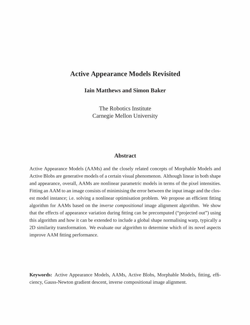
See Figure 1 for an example mesh that contains 68 vertices. AAMs allow linear shape variation.

This means that the shapes can be expressed as a base shapes0 plus a linear combination ofn

shape vectorssi:

s = s0 +n

∑

i=1

pisi. (2)

In this expression the coefficientspi are the shape parameters. Since we can always perform a

linear reparameterization, wherever necessary we assume that the vectorssi are orthonormal.

AAMs are normally computed from hand labelled training images. The standard approach is to

3

s0 s1 s2 s3

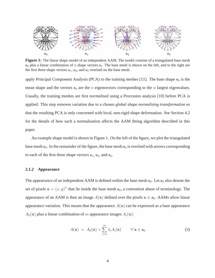
Figure 1: The linear shape model of an independent AAM. The model consists of a triangulated base meshs0 plus a linear combination ofn shape vectorssi. The base mesh is shown on the left, and to the right arethe first three shape vectorss1, s2, ands3 overlaid on the base mesh.

apply Principal Component Analysis (PCA) to the training meshes [11]. The base shapes0 is the

mean shape and the vectorss0 are then eigenvectors corresponding to then largest eigenvalues.

Usually, the training meshes are firstnormalisedusing a Procrustes analysis [10] before PCA is

applied. This step removes variation due to a chosenglobal shape normalising transformationso

that the resulting PCA is only concerned with local, non-rigid shape deformation. See Section 4.2

for the details of how such a normalisation affects the AAM fitting algorithm described in this

paper.

An example shape model is shown in Figure 1. On the left of the figure, we plot the triangulated

base meshs0. In the remainder of the figure, the base meshs0 is overlaid with arrows corresponding

to each of the first three shape vectorss1, s2, ands3.

2.1.2 Appearance

Theappearanceof an independent AAM is defined within the base meshs0. Let s0 also denote the

set of pixelsx = (x, y)T that lie inside the base meshs0, a convenient abuse of terminology. The

appearance of an AAM is then an imageA(x) defined over the pixelsx ∈ s0. AAMs allow linear

appearance variation. This means that the appearanceA(x) can be expressed as a base appearance

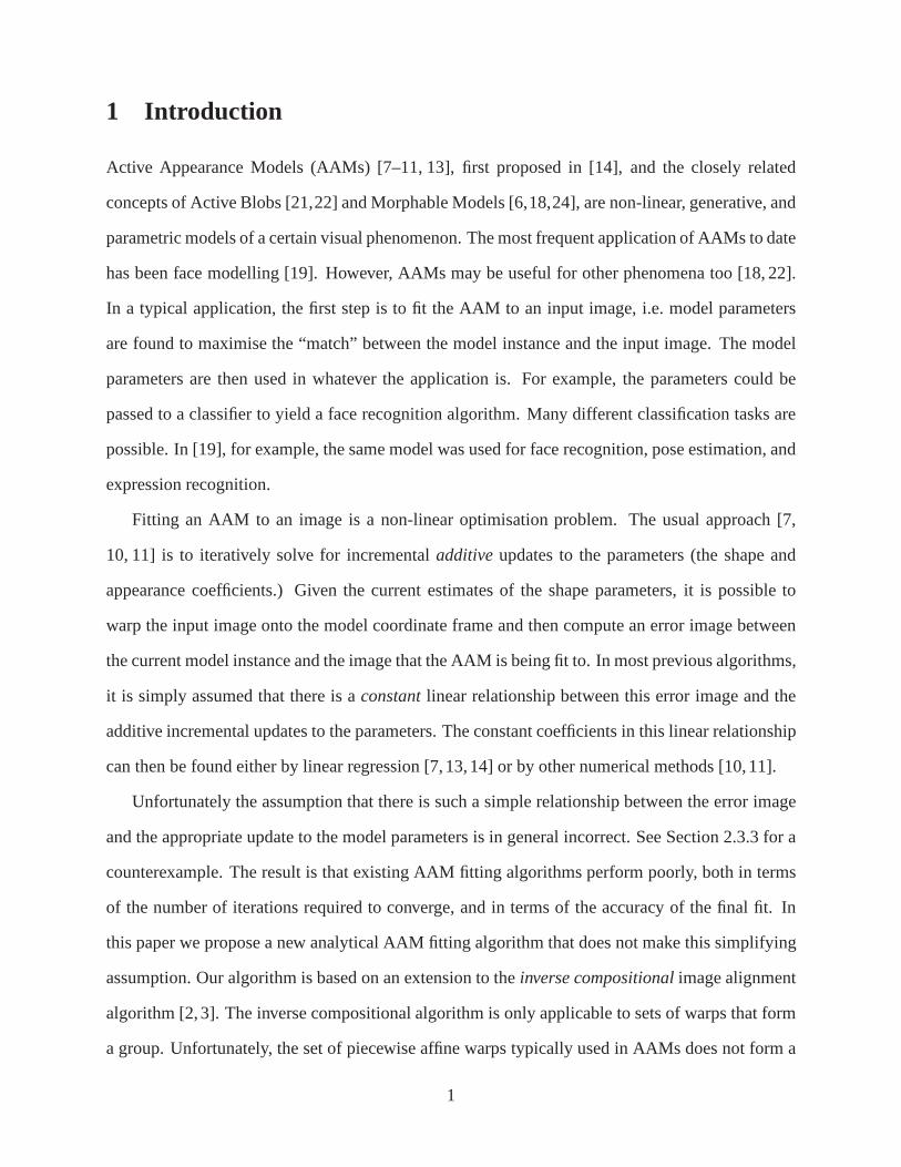
A0(x) plus a linear combination ofm appearance imagesAi(x):

A(x) = A0(x) +m

∑

i=1

λiAi(x) ∀ x ∈ s0 (3)

4

A0(x) A1(x) A2(x) A3(x)

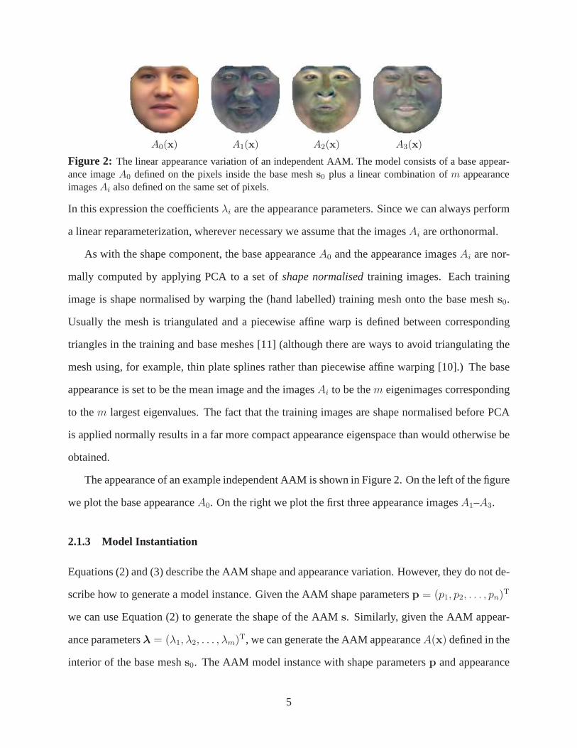
Figure 2: The linear appearance variation of an independent AAM. The model consists of a base appear-ance imageA0 defined on the pixels inside the base meshs0 plus a linear combination ofm appearanceimagesAi also defined on the same set of pixels.

In this expression the coefficientsλi are the appearance parameters. Since we can always perform

a linear reparameterization, wherever necessary we assumethat the imagesAi are orthonormal.

As with the shape component, the base appearanceA0 and the appearance imagesAi are nor-

mally computed by applying PCA to a set ofshape normalisedtraining images. Each training

image is shape normalised by warping the (hand labelled) training mesh onto the base meshs0.

Usually the mesh is triangulated and a piecewise affine warp is defined between corresponding

triangles in the training and base meshes [11] (although there are ways to avoid triangulating the

mesh using, for example, thin plate splines rather than piecewise affine warping [10].) The base

appearance is set to be the mean image and the imagesAi to be them eigenimages corresponding

to them largest eigenvalues. The fact that the training images are shape normalised before PCA

is applied normally results in a far more compact appearanceeigenspace than would otherwise be

obtained.

The appearance of an example independent AAM is shown in Figure 2. On the left of the figure

we plot the base appearanceA0. On the right we plot the first three appearance imagesA1–A3.

2.1.3 Model Instantiation

Equations (2) and (3) describe the AAM shape and appearance variation. However, they do not de-

scribe how to generate a model instance. Given the AAM shape parametersp = (p1, p2, . . . , pn)T

we can use Equation (2) to generate the shape of the AAMs. Similarly, given the AAM appear-

ance parametersλ = (λ1, λ2, . . . , λm)T, we can generate the AAM appearanceA(x) defined in the

interior of the base meshs0. The AAM model instance with shape parametersp and appearance

5

9.1s3

W(x;p)

Appearance,A

Shape,s

=

=

A0

AAM Model Instance

M(W(x;p))

s0 − +54s1 − . . .10s2

. . .256A3−351A2++ 3559A1

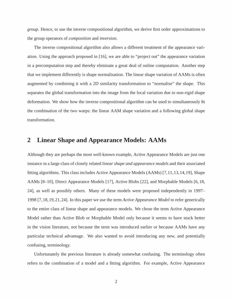
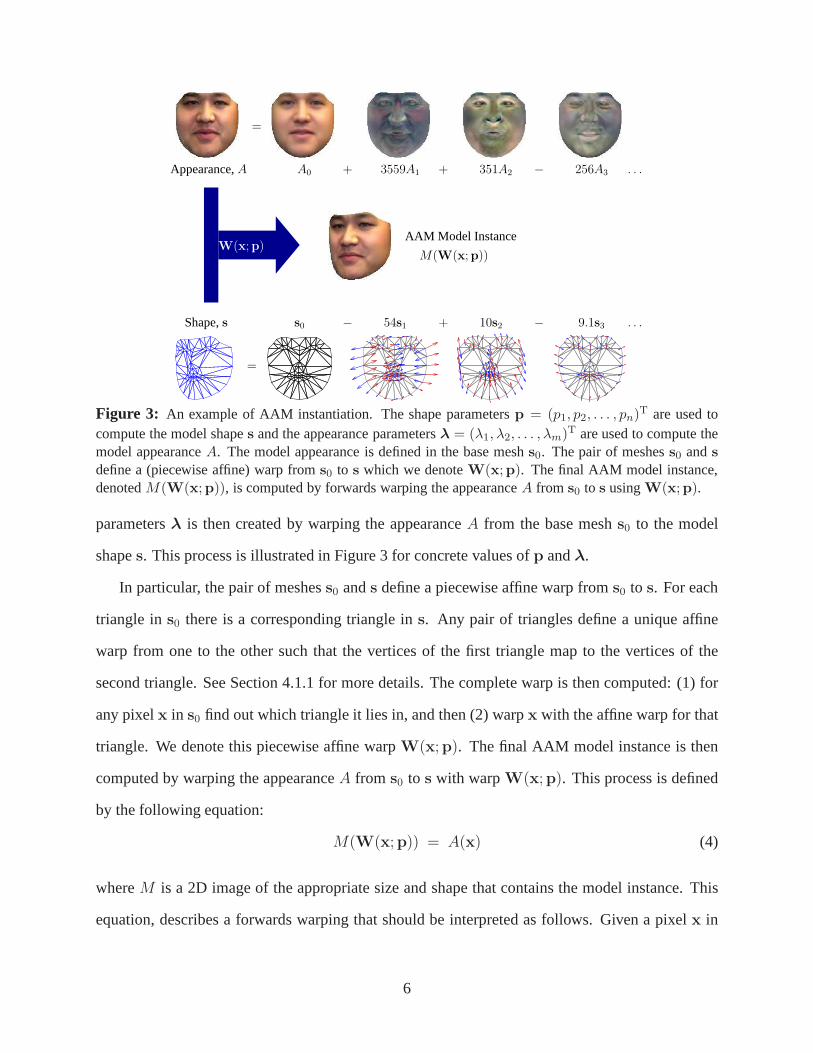
Figure 3: An example of AAM instantiation. The shape parametersp = (p1, p2, . . . , pn)T are used tocompute the model shapes and the appearance parametersλ = (λ1, λ2, . . . , λm)T are used to compute themodel appearanceA. The model appearance is defined in the base meshs0. The pair of meshess0 ands

define a (piecewise affine) warp froms0 to s which we denoteW(x;p). The final AAM model instance,denotedM(W(x;p)), is computed by forwards warping the appearanceA from s0 to s usingW(x;p).

parametersλ is then created by warping the appearanceA from the base meshs0 to the model

shapes. This process is illustrated in Figure 3 for concrete valuesof p andλ.

In particular, the pair of meshess0 ands define a piecewise affine warp froms0 to s. For each

triangle ins0 there is a corresponding triangle ins. Any pair of triangles define a unique affine

warp from one to the other such that the vertices of the first triangle map to the vertices of the

second triangle. See Section 4.1.1 for more details. The complete warp is then computed: (1) for

any pixelx in s0 find out which triangle it lies in, and then (2) warpx with the affine warp for that

triangle. We denote this piecewise affine warpW(x;p). The final AAM model instance is then

computed by warping the appearanceA from s0 to s with warpW(x;p). This process is defined

by the following equation:

M(W(x;p)) = A(x) (4)

whereM is a 2D image of the appropriate size and shape that contains the model instance. This

equation, describes a forwards warping that should be interpreted as follows. Given a pixelx in

6

s0, the destination of this pixel under the warp isW(x;p). The AAM modelM at pixelW(x;p)

in s is set to the appearanceA(x). Implementing this forwards warping to generate the model

instanceM without holes (see Figure 3) is actually somewhat tricky andis best performed by

backwards warping with the inverse warp froms to s0. Fortunately, in the AAM fitting algorithms,

only backwards warping froms onto the base meshs0 is needed. Finally, note that the piecewise

affine warping described in this section could be replaced with any other method of interpolating

between the mesh vertices. For example, thin plate splines could be used instead [10].

2.2 Combined AAMs

While independent AAMs have separate shapep and appearanceλ parameters,combinedAAMs

just use a single set of parametersc = (c1, c2, . . . , cl)T to parameterize shape:

s = s0 +l

∑

i=1

cisi (5)

and appearance:

A(x) = A0(x) +l

∑

i=1

ciAi(x). (6)

The shape and appearance parts of the model are therefore coupled. This coupling has a number

of disadvantages. For example, it means that we can no longerassume the vectorssi andAi(x)

are respectively orthonormal. It also restricts the choiceof fitting algorithm. See the discussion at

the end of this paper. On the other hand, combined AAMs have a number of advantages. First,

the combined formulation is more general and is a strict superset of the independent formulation.

To see this, setc = (p1, p2, . . . , pn, λ1, λ2, . . . , λm)T and choosesi andAi appropriately. Second,

combined AAMs often need less parameters to represent the same visual phenomenon to the same

degree of accuracy; i.e. in practicel ≤ m + n. Therefore fitting may be more efficient.

This second advantage is actually not very significant. Since we will “project out” the appear-

ance variation, as discussed in Section 4.1.5, the computational cost of our new algorithm is mainly

dependent on the number of shape parametersn and does not depend significantly on the number of

7

appearance parametersm. The computational reduction by usingl parameters rather thann+m pa-

rameters is therefore non-existent. For the same representational accuracy,l ≥ max(n, m). Hence,

our algorithm which uses independent AAMs and runs in timeO(n) is actually more efficient than

any for combined AAMs and which runs in timeO(l).

Combined AAMs are normally computed by taking an independent AAM and performing (a

third) Principal Component Analysis on the appropriately weighted training shapep and appear-

anceλ parameters. The shape and appearance parameters are then linearly reparameterized in

terms of the new eigenvectors of the combined PCA. See [11] for the details, although note that

the presentation there is somewhat different from the essentially equivalent presentation here.

2.3 Fitting AAMs

2.3.1 Fitting Goal

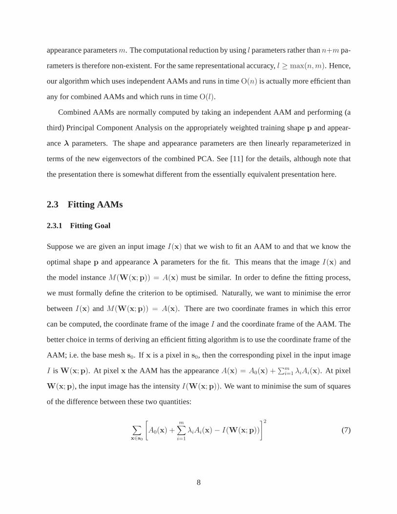
Suppose we are given an input imageI(x) that we wish to fit an AAM to and that we know the

optimal shapep and appearanceλ parameters for the fit. This means that the imageI(x) and

the model instanceM(W(x;p)) = A(x) must be similar. In order to define the fitting process,

we must formally define the criterion to be optimised. Naturally, we want to minimise the error

betweenI(x) andM(W(x;p)) = A(x). There are two coordinate frames in which this error

can be computed, the coordinate frame of the imageI and the coordinate frame of the AAM. The

better choice in terms of deriving an efficient fitting algorithm is to use the coordinate frame of the

AAM; i.e. the base meshs0. If x is a pixel ins0, then the corresponding pixel in the input image

I is W(x;p). At pixel x the AAM has the appearanceA(x) = A0(x) +∑m

i=1 λiAi(x). At pixel

W(x;p), the input image has the intensityI(W(x;p)). We want to minimise the sum of squares

of the difference between these two quantities:

∑

x∈s0

[

A0(x) +m

∑

i=1

λiAi(x)− I(W(x;p))

]2

(7)

8

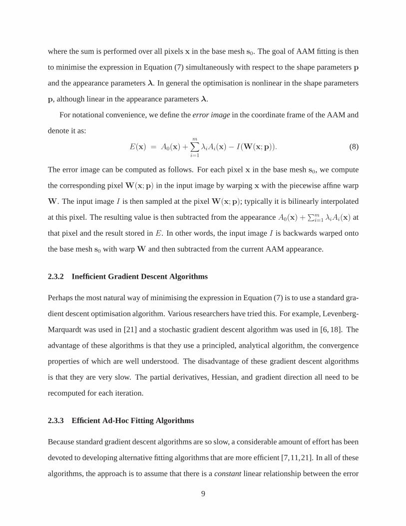
where the sum is performed over all pixelsx in the base meshs0. The goal of AAM fitting is then

to minimise the expression in Equation (7) simultaneously with respect to the shape parametersp

and the appearance parametersλ. In general the optimisation is nonlinear in the shape parameters

p, although linear in the appearance parametersλ.

For notational convenience, we define theerror imagein the coordinate frame of the AAM and

denote it as:

E(x) = A0(x) +m

∑

i=1

λiAi(x)− I(W(x;p)). (8)

The error image can be computed as follows. For each pixelx in the base meshs0, we compute

the corresponding pixelW(x;p) in the input image by warpingx with the piecewise affine warp

W. The input imageI is then sampled at the pixelW(x;p); typically it is bilinearly interpolated

at this pixel. The resulting value is then subtracted from the appearanceA0(x) +∑m

i=1 λiAi(x) at

that pixel and the result stored inE. In other words, the input imageI is backwards warped onto

the base meshs0 with warpW and then subtracted from the current AAM appearance.

2.3.2 Inefficient Gradient Descent Algorithms

Perhaps the most natural way of minimising the expression inEquation (7) is to use a standard gra-

dient descent optimisation algorithm. Various researchers have tried this. For example, Levenberg-

Marquardt was used in [21] and a stochastic gradient descentalgorithm was used in [6, 18]. The

advantage of these algorithms is that they use a principled,analytical algorithm, the convergence

properties of which are well understood. The disadvantage of these gradient descent algorithms

is that they are very slow. The partial derivatives, Hessian, and gradient direction all need to be

recomputed for each iteration.

2.3.3 Efficient Ad-Hoc Fitting Algorithms

Because standard gradient descent algorithms are so slow, aconsiderable amount of effort has been

devoted to developing alternative fitting algorithms that are more efficient [7,11,21]. In all of these

algorithms, the approach is to assume that there is aconstantlinear relationship between the error

9

imageE(x) andadditiveincrements to the shape and appearance parameters:

∆pi =∑

x∈s0

Ri(x)E(x) and ∆λi =∑

x∈s0

Si(x)E(x) (9)

whereRi(x) andSi(x) are constant images defined on the base meshs0. Here, constant means

that Ri(x) andSi(x) do not depend onpi or λi. This assumption is motivated by the fact that

almost all previous gradient descent algorithms boil down to computing∆pi and∆λi as linear

functions of the error image and then updatingpi ← pi + ∆pi andλi ← λi + ∆λi. However,

in previous gradient descent algorithms the equivalent ofRi(x) andSi(x) are not constant, but

instead depend on the AAM model parametersp andλ. It is because they depend on the current

model parameters that they have to be recomputed. In essence, this is why the gradient descent

algorithms are so inefficient.

To improve the efficiency, previous AAM fitting algorithms such as [7, 11, 21] have either ex-

plicitly or implicitly simply assumed thatRi(x) andSi(x) do notdepend on the model parameters.

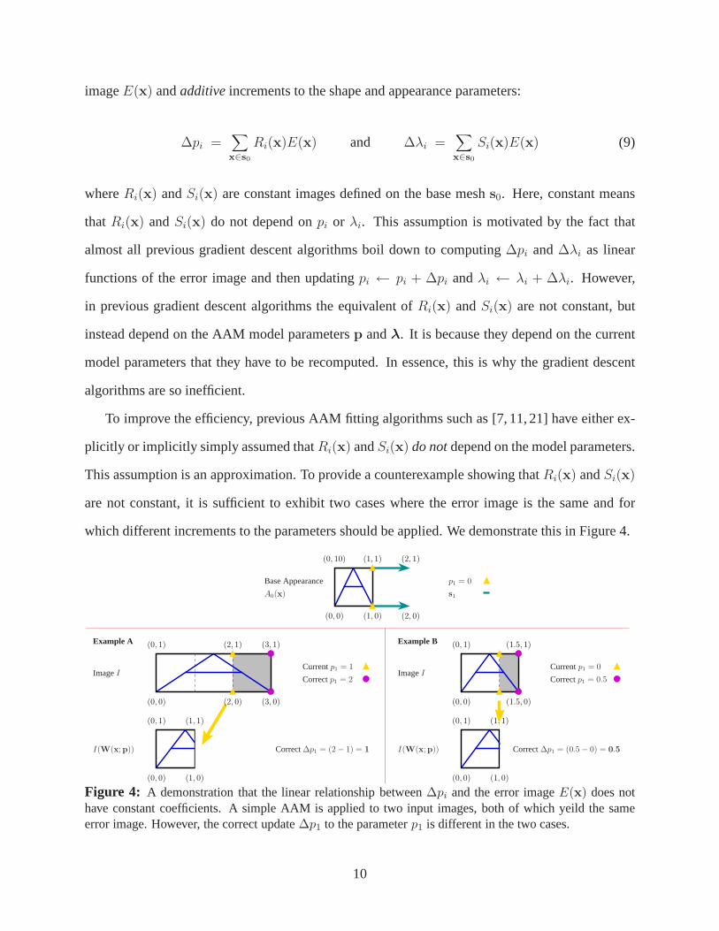
This assumption is an approximation. To provide a counterexample showing thatRi(x) andSi(x)

are not constant, it is sufficient to exhibit two cases where the error image is the same and for

which different increments to the parameters should be applied. We demonstrate this in Figure 4.

p1 = 0

s1

Example A

ImageICurrentp1 = 1

Correctp1 = 2

(0, 0)

(0, 1)

(1.5, 0)

(0, 0)

(0, 1)

(1, 0)

(1, 1)

(1.5, 1)

Currentp1 = 0

Correctp1 = 0.5

I(W(x;p)) Correct∆p1 = (0.5− 0) = 0.5Correct∆p1 = (2− 1) = 1

(0, 0)

(0, 1)

(3, 0)

(3, 1)(2, 1)

(0, 0) (1, 0)

(1, 1)

Example B

(0, 0)

(1, 1)(0, 10)

(1, 0) (2, 0)

(2, 1)

Base Appearance

A0(x)

(0, 1)

ImageI

(2, 0)

I(W(x;p))

Figure 4: A demonstration that the linear relationship between∆pi and the error imageE(x) does nothave constant coefficients. A simple AAM is applied to two input images, both of which yeild the sameerror image. However, the correct update∆p1 to the parameterp1 is different in the two cases.

10

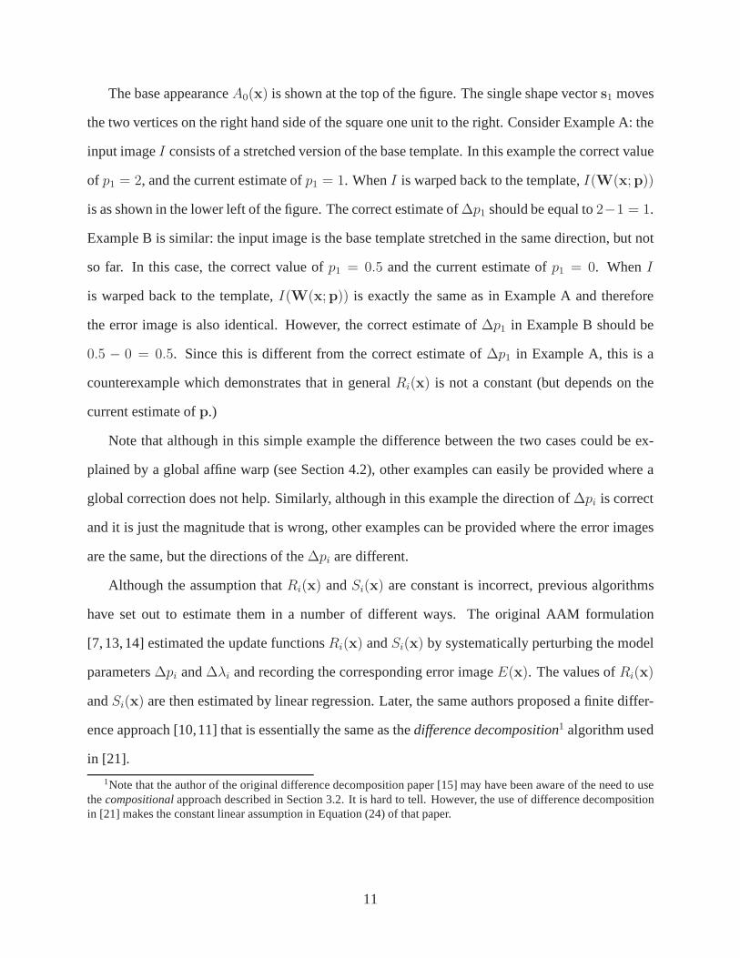
The base appearanceA0(x) is shown at the top of the figure. The single shape vectors1 moves

the two vertices on the right hand side of the square one unit to the right. Consider Example A: the

input imageI consists of a stretched version of the base template. In thisexample the correct value

of p1 = 2, and the current estimate ofp1 = 1. WhenI is warped back to the template,I(W(x;p))

is as shown in the lower left of the figure. The correct estimate of∆p1 should be equal to2−1 = 1.

Example B is similar: the input image is the base template stretched in the same direction, but not

so far. In this case, the correct value ofp1 = 0.5 and the current estimate ofp1 = 0. WhenI

is warped back to the template,I(W(x;p)) is exactly the same as in Example A and therefore

the error image is also identical. However, the correct estimate of∆p1 in Example B should be

0.5 − 0 = 0.5. Since this is different from the correct estimate of∆p1 in Example A, this is a

counterexample which demonstrates that in generalRi(x) is not a constant (but depends on the

current estimate ofp.)

Note that although in this simple example the difference between the two cases could be ex-

plained by a global affine warp (see Section 4.2), other examples can easily be provided where a

global correction does not help. Similarly, although in this example the direction of∆pi is correct

and it is just the magnitude that is wrong, other examples canbe provided where the error images

are the same, but the directions of the∆pi are different.

Although the assumption thatRi(x) andSi(x) are constant is incorrect, previous algorithms

have set out to estimate them in a number of different ways. The original AAM formulation

[7,13,14] estimated the update functionsRi(x) andSi(x) by systematically perturbing the model

parameters∆pi and∆λi and recording the corresponding error imageE(x). The values ofRi(x)

andSi(x) are then estimated by linear regression. Later, the same authors proposed a finite differ-

ence approach [10,11] that is essentially the same as thedifference decomposition1 algorithm used

in [21].

1Note that the author of the original difference decomposition paper [15] may have been aware of the need to usethecompositionalapproach described in Section 3.2. It is hard to tell. However, the use of difference decompositionin [21] makes the constant linear assumption in Equation (24) of that paper.

11

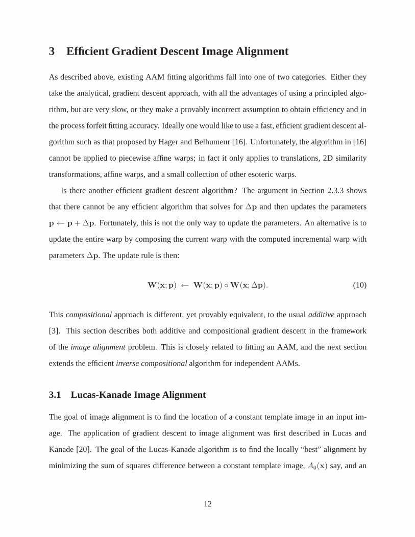
3 Efficient Gradient Descent Image Alignment

As described above, existing AAM fitting algorithms fall into one of two categories. Either they

take the analytical, gradient descent approach, with all the advantages of using a principled algo-

rithm, but are very slow, or they make a provably incorrect assumption to obtain efficiency and in

the process forfeit fitting accuracy. Ideally one would liketo use a fast, efficient gradient descent al-

gorithm such as that proposed by Hager and Belhumeur [16]. Unfortunately, the algorithm in [16]

cannot be applied to piecewise affine warps; in fact it only applies to translations, 2D similarity

transformations, affine warps, and a small collection of other esoteric warps.

Is there another efficient gradient descent algorithm? The argument in Section 2.3.3 shows

that there cannot be any efficient algorithm that solves for∆p and then updates the parameters

p ← p + ∆p. Fortunately, this is not the only way to update the parameters. An alternative is to

update the entire warp by composing the current warp with thecomputed incremental warp with

parameters∆p. The update rule is then:

W(x;p) ← W(x;p) ◦W(x; ∆p). (10)

This compositionalapproach is different, yet provably equivalent, to the usual additiveapproach

[3]. This section describes both additive and compositional gradient descent in the framework

of the image alignmentproblem. This is closely related to fitting an AAM, and the next section

extends the efficientinverse compositionalalgorithm for independent AAMs.

3.1 Lucas-Kanade Image Alignment

The goal of image alignment is to find the location of a constant template image in an input im-

age. The application of gradient descent to image alignmentwas first described in Lucas and

Kanade [20]. The goal of the Lucas-Kanade algorithm is to findthe locally “best” alignment by

minimizing the sum of squares difference between a constanttemplate image,A0(x) say, and an

12

example imageI(x) with respect to the warp parametersp:

∑

x

[A0(x)− I(W(x;p))]2. (11)

Note the similarity with Equation (7). As in Section 2,W(x;p) is a warp that maps the pixelsx

from the template (i.e. the base mesh) image to the input image and has parametersp. Note that

I(W(x;p)) is an image with the same dimensions as the template; it is theinput imageI warped

backwards onto the same coordinate frame as the template.

Solving forp is a nonlinear optimisation problem. This is true even ifW(x;p) is linear inp

because, in general, the pixel valuesI(x) are nonlinear in (and essentially unrelated to) the pixel

coordinatesx. To linearize the problem, the Lucas-Kanade algorithm assumes that an initial esti-

mate ofp is known and then iteratively solves for increments to the parameters∆p; i.e. minimise:

∑

x

[A0(x)− I(W(x;p + ∆p))]2 (12)

with respect to∆p and then updatep← p+∆p. The expression in Equation (12) can be linearized

aboutp using a Taylor series expansion to give:

∑

x

[

A0(x)− I(W(x;p))−∇I∂W

∂p∆p

]2

, (13)

where∇I is thegradientof the image evaluated atW(x;p), and∂W

∂pis theJacobianof the warp

evaluated atp. The closed form solution of Equation (13) for∆p is:

∆p = H−1∑

x

[

∇I∂W

∂p

]T

[A0(x)− I(W(x;p))] (14)

whereH is the Gauss-Newton approximation to theHessianmatrix:

H =∑

x

[

∇I∂W

∂p

]T [

∇I∂W

∂p

]

. (15)

13

(Known)

W(x;p)

I(x)

W(x;p + ∆p)

A0(x)

(Estimated)

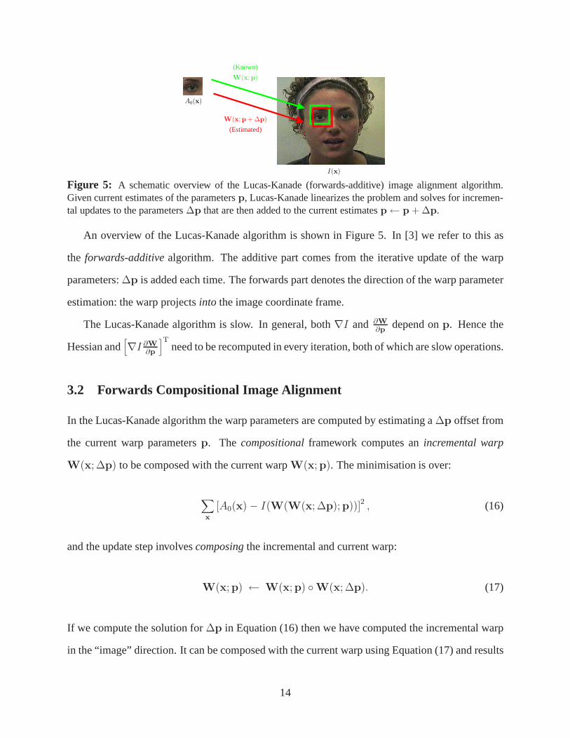
Figure 5: A schematic overview of the Lucas-Kanade (forwards-additive) image alignment algorithm.Given current estimates of the parametersp, Lucas-Kanade linearizes the problem and solves for incremen-tal updates to the parameters∆p that are then added to the current estimatesp← p + ∆p.

An overview of the Lucas-Kanade algorithm is shown in Figure5. In [3] we refer to this as

the forwards-additivealgorithm. The additive part comes from the iterative update of the warp

parameters:∆p is added each time. The forwards part denotes the direction of the warp parameter

estimation: the warp projectsinto the image coordinate frame.

The Lucas-Kanade algorithm is slow. In general, both∇I and ∂W

∂pdepend onp. Hence the

Hessian and[

∇I ∂W∂p

]Tneed to be recomputed in every iteration, both of which are slow operations.

3.2 Forwards Compositional Image Alignment

In the Lucas-Kanade algorithm the warp parameters are computed by estimating a∆p offset from

the current warp parametersp. The compositionalframework computes anincremental warp

W(x; ∆p) to be composed with the current warpW(x;p). The minimisation is over:

∑

x

[A0(x)− I(W(W(x; ∆p);p))]2 , (16)

and the update step involvescomposingthe incremental and current warp:

W(x;p) ← W(x;p) ◦W(x; ∆p). (17)

If we compute the solution for∆p in Equation (16) then we have computed the incremental warp

in the “image” direction. It can be composed with the currentwarp using Equation (17) and results

14

in the forwards compositionalalgorithm [3]. This algorithm was also used in [23]. Taking the

Taylor series expansion of Equation (16) gives:

∑

x

[

A0(x)− I(W(W(x; 0);p))−∇I(W(x;p))∂W

∂p∆p

]2

. (18)

At this point we assume thatp = 0 is the identity warp; i.e.W(x; 0) = x. There are then

two differences between Equation (18) and Equation (13). First, the gradient is computed on

I(W(x;p)). Second, the Jacobian is evaluated at(x; 0) and therefore is a constant that can be

precomputed. The composition update step is computationally more costly than the update step

for an additive algorithm, but this is offset by not having tocompute the Jacobian∂W

∂pin each

iteration.

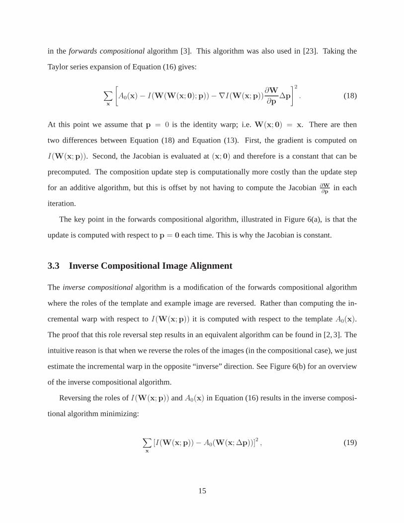
The key point in the forwards compositional algorithm, illustrated in Figure 6(a), is that the

update is computed with respect top = 0 each time. This is why the Jacobian is constant.

3.3 Inverse Compositional Image Alignment

The inverse compositionalalgorithm is a modification of the forwards compositional algorithm

where the roles of the template and example image are reversed. Rather than computing the in-

cremental warp with respect toI(W(x;p)) it is computed with respect to the templateA0(x).

The proof that this role reversal step results in an equivalent algorithm can be found in [2, 3]. The

intuitive reason is that when we reverse the roles of the images (in the compositional case), we just

estimate the incremental warp in the opposite “inverse” direction. See Figure 6(b) for an overview

of the inverse compositional algorithm.

Reversing the roles ofI(W(x;p)) andA0(x) in Equation (16) results in the inverse composi-

tional algorithm minimizing:

∑

x

[I(W(x;p))− A0(W(x; ∆p))]2 , (19)

15

(Estimated)

W(x; ∆p)

A0(x)

W(x;p)

I(x)

(Known)I(W(x;p))

W(x;p) ◦W(x; ∆p)

(Update)

(Estimated)

W(x; ∆p)

A0(x)

W(x;p)

I(x)

I(W(x;p))

W(x;p) ◦W(x; ∆p)−1

(Update)

(Known)

(a) Forwards Compositional (b) Inverse Compositional

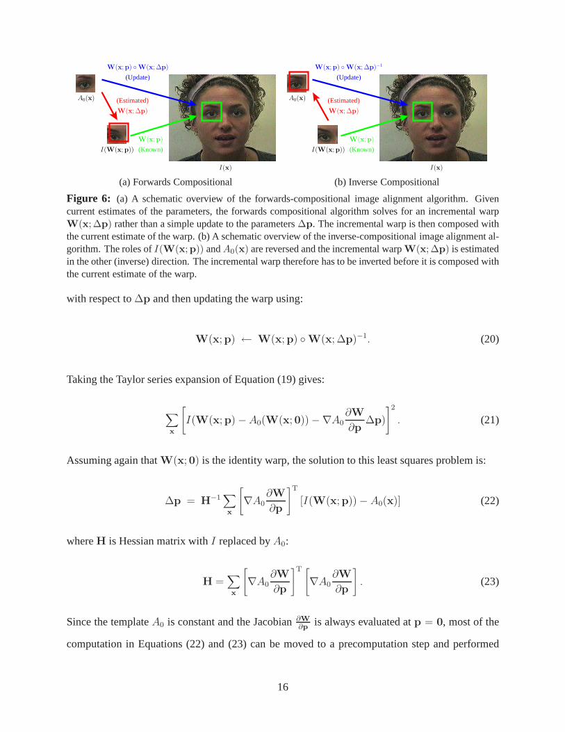
Figure 6: (a) A schematic overview of the forwards-compositional image alignment algorithm. Givencurrent estimates of the parameters, the forwards compositional algorithm solves for an incremental warpW(x;∆p) rather than a simple update to the parameters∆p. The incremental warp is then composed withthe current estimate of the warp. (b) A schematic overview ofthe inverse-compositional image alignment al-gorithm. The roles ofI(W(x;p)) andA0(x) are reversed and the incremental warpW(x;∆p) is estimatedin the other (inverse) direction. The incremental warp therefore has to be inverted before it is composed withthe current estimate of the warp.

with respect to∆p and then updating the warp using:

W(x;p) ← W(x;p) ◦W(x; ∆p)−1. (20)

Taking the Taylor series expansion of Equation (19) gives:

∑

x

[

I(W(x;p)−A0(W(x; 0))−∇A0∂W

∂p∆p)

]2

. (21)

Assuming again thatW(x; 0) is the identity warp, the solution to this least squares problem is:

∆p = H−1∑

x

[

∇A0∂W

∂p

]T

[I(W(x;p))− A0(x)] (22)

whereH is Hessian matrix withI replaced byA0:

H =∑

x

[

∇A0∂W

∂p

]T [

∇A0∂W

∂p

]

. (23)

Since the templateA0 is constant and the Jacobian∂W∂p

is always evaluated atp = 0, most of the

computation in Equations (22) and (23) can be moved to a precomputation step and performed

16

The Inverse Compositional Algorithm

Pre-compute:

(3) Evaluate the gradient∇A0 of the templateA0(x)

(4) Evaluate the Jacobian∂W∂p

at (x;0)

(5) Compute the steepest descent images∇A0∂W∂p

(6) Compute the Hessian matrix using Equation (23)

Iterate Until Converged:

(1) WarpI with W(x;p) to computeI(W(x;p))

(2) Compute the error imageI(W(x;p)) −A0(x)

(7) Compute∑

x[∇A0∂W∂p

]T[I(W(x;p)) −A0(x)]

(8) Compute∆p using Equation (22)(9) Update the warpW(x;p)←W(x;p) ◦W(x;∆p)−1

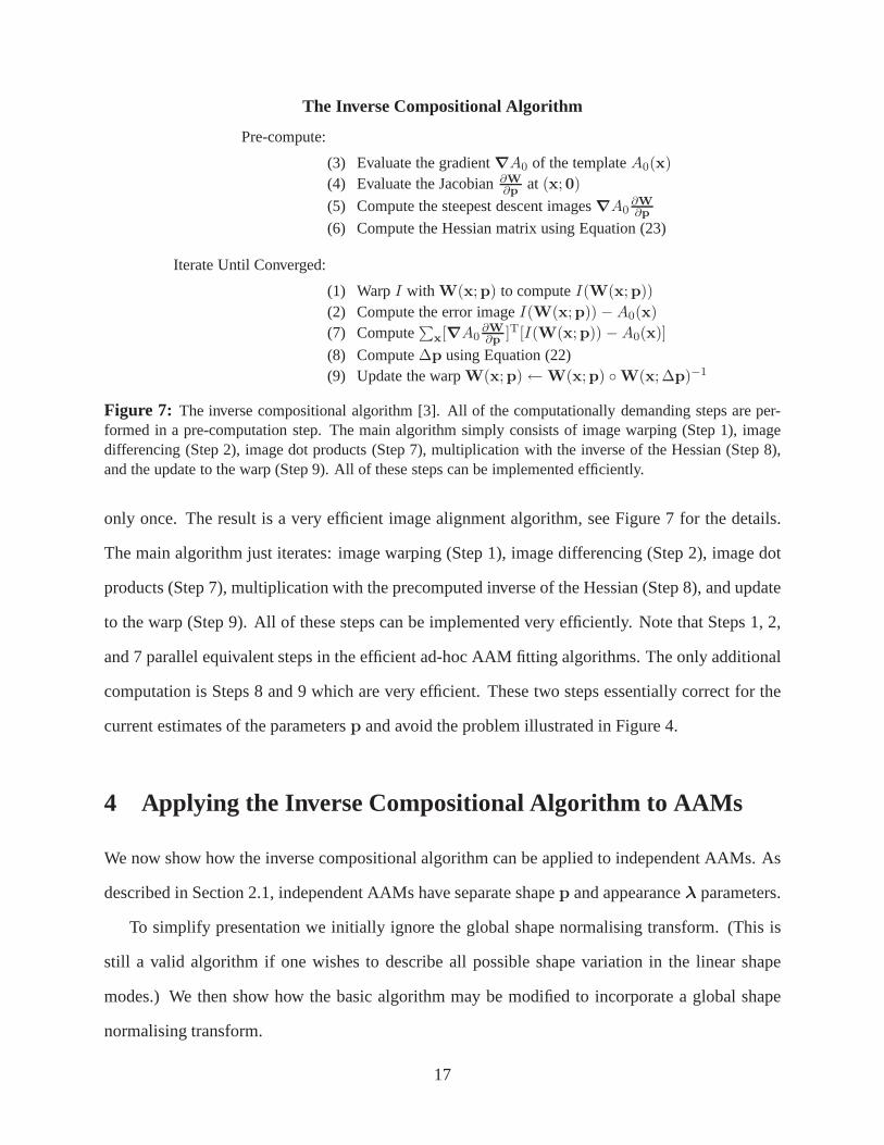
Figure 7: The inverse compositional algorithm [3]. All of the computationally demanding steps are per-formed in a pre-computation step. The main algorithm simplyconsists of image warping (Step 1), imagedifferencing (Step 2), image dot products (Step 7), multiplication with the inverse of the Hessian (Step 8),and the update to the warp (Step 9). All of these steps can be implemented efficiently.

only once. The result is a very efficient image alignment algorithm, see Figure 7 for the details.

The main algorithm just iterates: image warping (Step 1), image differencing (Step 2), image dot

products (Step 7), multiplication with the precomputed inverse of the Hessian (Step 8), and update

to the warp (Step 9). All of these steps can be implemented very efficiently. Note that Steps 1, 2,

and 7 parallel equivalent steps in the efficient ad-hoc AAM fitting algorithms. The only additional

computation is Steps 8 and 9 which are very efficient. These two steps essentially correct for the

current estimates of the parametersp and avoid the problem illustrated in Figure 4.

4 Applying the Inverse Compositional Algorithm to AAMs

We now show how the inverse compositional algorithm can be applied to independent AAMs. As

described in Section 2.1, independent AAMs have separate shapep and appearanceλ parameters.

To simplify presentation we initially ignore the global shape normalising transform. (This is

still a valid algorithm if one wishes to describe all possible shape variation in the linear shape

modes.) We then show how the basic algorithm may be modified toincorporate a global shape

normalising transform.

17

Corresponding Triangle in Meshs

(x, y)TW(x;p)α

α

W(x;p)

(xk, yk)T

(x0k, y

0k)

T

(x0j , y

0j )

T(xj , yj)

T

(xi, yi)T

(x0i , y

0i )

T

ββ

Triangle in Base Meshs0

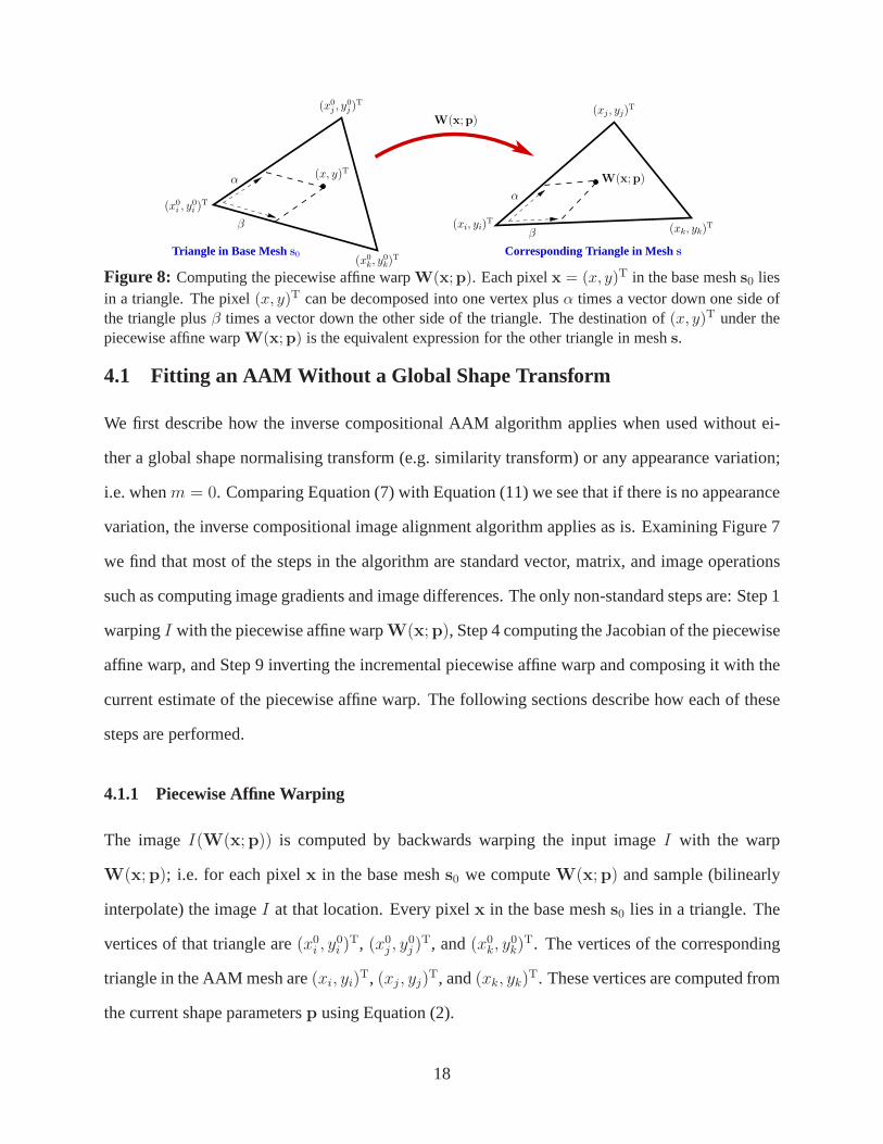
Figure 8: Computing the piecewise affine warpW(x;p). Each pixelx = (x, y)T in the base meshs0 liesin a triangle. The pixel(x, y)T can be decomposed into one vertex plusα times a vector down one side ofthe triangle plusβ times a vector down the other side of the triangle. The destination of (x, y)T under thepiecewise affine warpW(x;p) is the equivalent expression for the other triangle in meshs.

4.1 Fitting an AAM Without a Global Shape Transform

We first describe how the inverse compositional AAM algorithm applies when used without ei-

ther a global shape normalising transform (e.g. similaritytransform) or any appearance variation;

i.e. whenm = 0. Comparing Equation (7) with Equation (11) we see that if there is no appearance

variation, the inverse compositional image alignment algorithm applies as is. Examining Figure 7

we find that most of the steps in the algorithm are standard vector, matrix, and image operations

such as computing image gradients and image differences. The only non-standard steps are: Step 1

warpingI with the piecewise affine warpW(x;p), Step 4 computing the Jacobian of the piecewise

affine warp, and Step 9 inverting the incremental piecewise affine warp and composing it with the

current estimate of the piecewise affine warp. The followingsections describe how each of these

steps are performed.

4.1.1 Piecewise Affine Warping

The imageI(W(x;p)) is computed by backwards warping the input imageI with the warp

W(x;p); i.e. for each pixelx in the base meshs0 we computeW(x;p) and sample (bilinearly

interpolate) the imageI at that location. Every pixelx in the base meshs0 lies in a triangle. The

vertices of that triangle are(x0i , y

0i )

T, (x0j , y

0j )

T, and(x0k, y

0k)

T. The vertices of the corresponding

triangle in the AAM mesh are(xi, yi)T, (xj , yj)

T, and(xk, yk)T. These vertices are computed from

the current shape parametersp using Equation (2).

18

One way to implement the piecewise affine warp is illustratedin Figure 8. Consider the pixel

x = (x, y)T in the triangle(x0i , y

0i )

T, (x0j , y

0j )

T, and(x0k, y

0k)

T in the base meshs0. This pixel can

be uniquely expressed as:

x = (x, y)T = (x0i , y

0i )

T + α[

(x0j , y

0j )

T − (x0i , y

0i )

T]

+ β[

(x0k, y

0k)

T − (x0i , y

0i )

T]

(24)

where:

α =(x− x0

i )(y0k − y0

i )− (y − y0i )(x

0k − x0

i )

(x0j − x0

i )(y0k − y0

i )− (y0j − y0

i )(x0k − x0

i )(25)

and:

β =(y − y0

i )(x0j − x0

i )− (x− x0i )(y

0j − y0

i )

(x0j − x0

i )(y0k − y0

i )− (y0j − y0

i )(x0k − x0

i ). (26)

The result of applying the piecewise affine warp is then:

W(x;p) = (xi, yi)T + α

[

(xj , yj)T − (xi, yi)

T]

+ β[

(xk, yk)T − (xi, yi)

T]

(27)

where(xi, yi)T, (xj , yj)

T, and(xk, yk)T are the vertices of the corresponding triangle ins. To-

gether, Equation (25), (26), and (27) constitute a simple affine warp:

W(x;p) = (a1 + a2 · x + a3 · y, a4 + a5 · x + a6 · y)T. (28)

The 6 parameters of this warp(a1, a2, a3, a4, a5, a6) can easily be computed from the shape pa-

rametersp by combining Equations (2), (25), (26), and (27). This computation only needs to be

performed once per triangle, not once per pixel. To implement the piecewise affine warp efficiently,

the computation should be structured:

• Givenp compute(xi, yi)T for all vertices ins.

• Compute(a1, a2, a3, a4, a5, a6) for each triangle.

• For each pixelx in the meshs0, lookup the triangle thatx lies in and then lookup thecorresponding values of(a1, a2, a3, a4, a5, a6).

• Finally, computeW(x;p) using Equation (28).

19

x

y

∂W∂x1

∂W∂y1

∂W∂x2

∂W∂y2

∂W∂x3

∂W∂y3

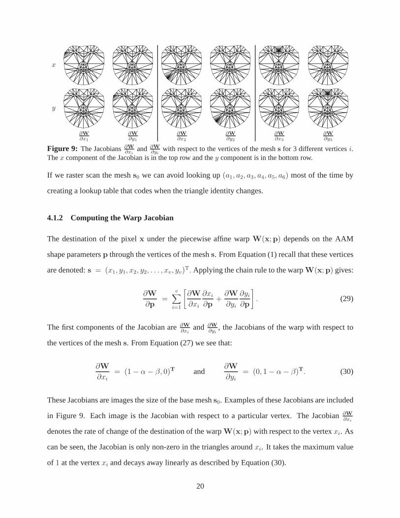
Figure 9: The Jacobians∂W∂xi

and ∂W∂yi

with respect to the vertices of the meshs for 3 different verticesi.Thex component of the Jacobian is in the top row and they component is in the bottom row.

If we raster scan the meshs0 we can avoid looking up(a1, a2, a3, a4, a5, a6) most of the time by

creating a lookup table that codes when the triangle identity changes.

4.1.2 Computing the Warp Jacobian

The destination of the pixelx under the piecewise affine warpW(x;p) depends on the AAM

shape parametersp through the vertices of the meshs. From Equation (1) recall that these vertices

are denoted:s = (x1, y1, x2, y2, . . . , xv, yv)T. Applying the chain rule to the warpW(x;p) gives:

∂W

∂p=

v∑

i=1

[

∂W

∂xi

∂xi

∂p+

∂W

∂yi

∂yi

∂p

]

. (29)

The first components of the Jacobian are∂W

∂xiand ∂W

∂yi, the Jacobians of the warp with respect to

the vertices of the meshs. From Equation (27) we see that:

∂W

∂xi

= (1− α− β, 0)T and∂W

∂yi

= (0, 1− α− β)T. (30)

These Jacobians are images the size of the base meshs0. Examples of these Jacobians are included

in Figure 9. Each image is the Jacobian with respect to a particular vertex. The Jacobian∂W∂xi

denotes the rate of change of the destination of the warpW(x;p) with respect to the vertexxi. As

can be seen, the Jacobian is only non-zero in the triangles aroundxi. It takes the maximum value

of 1 at the vertexxi and decays away linearly as described by Equation (30).

20

x

y

p1 p2 p3

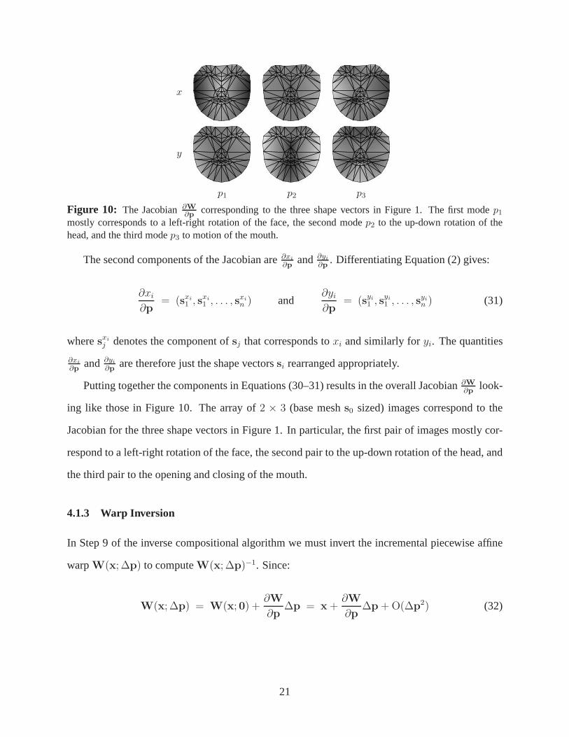
Figure 10: The Jacobian∂W∂p

corresponding to the three shape vectors in Figure 1. The first modep1

mostly corresponds to a left-right rotation of the face, thesecond modep2 to the up-down rotation of thehead, and the third modep3 to motion of the mouth.

The second components of the Jacobian are∂xi

∂pand ∂yi

∂p. Differentiating Equation (2) gives:

∂xi

∂p= (sxi

1 , sxi

1 , . . . , sxi

n ) and∂yi

∂p= (syi

1 , syi

1 , . . . , syi

n ) (31)

wheresxi

j denotes the component ofsj that corresponds toxi and similarly foryi. The quantities

∂xi

∂pand ∂yi

∂pare therefore just the shape vectorssi rearranged appropriately.

Putting together the components in Equations (30–31) results in the overall Jacobian∂W∂p

look-

ing like those in Figure 10. The array of2 × 3 (base meshs0 sized) images correspond to the

Jacobian for the three shape vectors in Figure 1. In particular, the first pair of images mostly cor-

respond to a left-right rotation of the face, the second pairto the up-down rotation of the head, and

the third pair to the opening and closing of the mouth.

4.1.3 Warp Inversion

In Step 9 of the inverse compositional algorithm we must invert the incremental piecewise affine

warpW(x; ∆p) to computeW(x; ∆p)−1. Since:

W(x; ∆p) = W(x; 0) +∂W

∂p∆p = x +

∂W

∂p∆p + O(∆p2) (32)

21

(remember thatW(x; 0) = x is the identity warp) we therefore have:

W(x; ∆p) ◦W(x;−∆p) = x−∂W

∂p∆p +

∂W

∂p∆p = x + O(∆p2). (33)

It therefore follows that to first order in∆p:

W(x; ∆p)−1 = W(x;−∆p). (34)

Note that the two Jacobians in Equation (33) are not evaluated at exactly the same location,

but since they are evaluated at pointsO(∆p) apart, they are equal to zeroth order in∆p. Since

the difference is multiplied by∆p we can ignore the first and higher order terms. Also note

that the composition of two warps is not strictly defined and so the argument in Equation (33) is

informal. The essence of the argument is correct, however. Once we have the derived the first

order approximation to the composition of two piecewise affine warps below, we can then use that

definition of composition in the argument above. The result is that the warpW(x;−∆p) followed

by the warpW(x; ∆p) is equal to the identity warp to first order in∆p.

4.1.4 Composing the Incremental Warp with the Current Warp Estimate

After we have inverted the piecewise affine warpW(x; ∆p) to computeW(x; ∆p)−1 in Step 9 we

must compose the result with the current warpW(x;p) to obtainW(x;p) ◦W(x; ∆p)−1. Given

the current estimate of the parametersp the current mesh vertex locationss = (x1, y1, . . . , xv, yv)T

can be computed using Equation (2). From the previous section, the parameters ofW(x; ∆p)−1

are−∆p. Given these parameters, we can use Equation (2) again to estimate the corresponding

changes to the base mesh vertex locations:

∆s0 = −n

∑

i=1

∆pisi (35)

22

Affine Warp

Base Meshs0

(∆xi, ∆yi)T(∆x0

i , ∆y0i )

T

(x0i , y

0i )

T+ (xi, yi)T+

(x0i , y

0i )

T (xi, yi)T

Current Mesh s

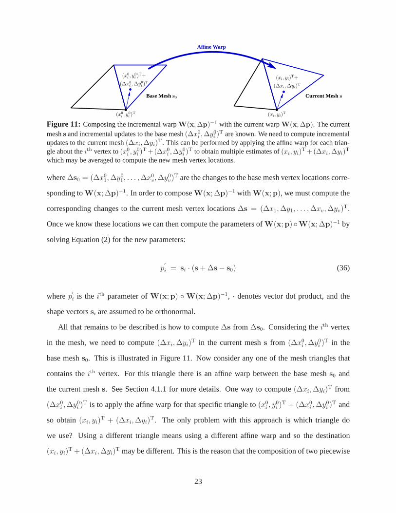
Figure 11: Composing the incremental warpW(x;∆p)−1 with the current warpW(x;∆p). The currentmeshs and incremental updates to the base mesh(∆x0

i ,∆y0i )

T are known. We need to compute incrementalupdates to the current mesh(∆xi,∆yi)

T. This can be performed by applying the affine warp for each trian-gle about theith vertex to(x0

i , y0i )

T +(∆x0i ,∆y0

i )T to obtain multiple estimates of(xi, yi)

T +(∆xi,∆yi)T

which may be averaged to compute the new mesh vertex locations.

where∆s0 = (∆x01, ∆y0

1, . . . , ∆x0v, ∆y0

v)T are the changes to the base mesh vertex locations corre-

sponding toW(x; ∆p)−1. In order to composeW(x; ∆p)−1 with W(x;p), we must compute the

corresponding changes to the current mesh vertex locations∆s = (∆x1, ∆y1, . . . , ∆xv, ∆yv)T.

Once we know these locations we can then compute the parameters ofW(x;p) ◦W(x; ∆p)−1 by

solving Equation (2) for the new parameters:

p′

i = si · (s + ∆s− s0) (36)

wherep′

i is the ith parameter ofW(x;p) ◦W(x; ∆p)−1, · denotes vector dot product, and the

shape vectorssi are assumed to be orthonormal.

All that remains to be described is how to compute∆s from ∆s0. Considering theith vertex

in the mesh, we need to compute(∆xi, ∆yi)T in the current meshs from (∆x0

i , ∆y0i )

T in the

base meshs0. This is illustrated in Figure 11. Now consider any one of themesh triangles that

contains theith vertex. For this triangle there is an affine warp between the base meshs0 and

the current meshs. See Section 4.1.1 for more details. One way to compute(∆xi, ∆yi)T from

(∆x0i , ∆y0

i )T is to apply the affine warp for that specific triangle to(x0

i , y0i )

T + (∆x0i , ∆y0

i )T and

so obtain(xi, yi)T + (∆xi, ∆yi)

T. The only problem with this approach is which triangle do

we use? Using a different triangle means using a different affine warp and so the destination

(xi, yi)T + (∆xi, ∆yi)

T may be different. This is the reason that the composition of two piecewise

23

affine warps is hard to define. In general there will be severaltriangles that share theith vertex.

One possibility is to use the triangle that contains the point (x0i , y

0i )

T +(∆x0i , ∆y0

i )T. The problem

with this approach is that the point could lie outside the base meshs0. Instead we compute the

destination(xi, yi)T + (∆xi, ∆yi)

T for every triangle that shares theith vertex and then average

the result. This will tend to smooth the warp at each vertex, but that is desirable anyway.

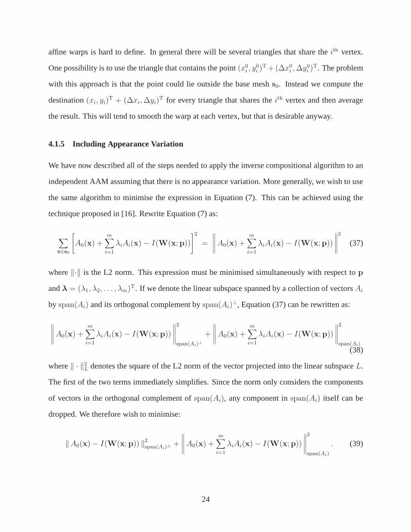
4.1.5 Including Appearance Variation

We have now described all of the steps needed to apply the inverse compositional algorithm to an

independent AAM assuming that there is no appearance variation. More generally, we wish to use

the same algorithm to minimise the expression in Equation (7). This can be achieved using the

technique proposed in [16]. Rewrite Equation (7) as:

∑

x∈s0

[

A0(x) +m

∑

i=1

λiAi(x)− I(W(x;p))

]2

=

∥

∥

∥

∥

∥

A0(x) +m

∑

i=1

λiAi(x)− I(W(x;p))

∥

∥

∥

∥

∥

2

(37)

where‖·‖ is the L2 norm. This expression must be minimised simultaneously with respect top

andλ = (λ1, λ2, . . . , λm)T. If we denote the linear subspace spanned by a collection of vectorsAi

by span(Ai) and its orthogonal complement byspan(Ai)⊥, Equation (37) can be rewritten as:

∥

∥

∥

∥

∥

A0(x) +m

∑

i=1

λiAi(x)− I(W(x;p))

∥

∥

∥

∥

∥

2

span(Ai)⊥

+

∥

∥

∥

∥

∥

A0(x) +m

∑

i=1

λiAi(x)− I(W(x;p))

∥

∥

∥

∥

∥

2

span(Ai)

(38)

where‖ · ‖2L denotes the square of the L2 norm of the vector projected intothe linear subspaceL.

The first of the two terms immediately simplifies. Since the norm only considers the components

of vectors in the orthogonal complement ofspan(Ai), any component inspan(Ai) itself can be

dropped. We therefore wish to minimise:

‖A0(x)− I(W(x;p)) ‖2span(Ai)⊥+

∥

∥

∥

∥

∥

A0(x) +m

∑

i=1

λiAi(x)− I(W(x;p))

∥

∥

∥

∥

∥

2

span(Ai)

. (39)

24

The first of these two terms does not depend uponλi. For anyp, the minimum value of the second

term is always0. Therefore the minimum value can be found sequentially by first minimising the

first term with respect top alone, and then using that optimal value ofp as a constant to minimise

the second term with respect to theλi. Assuming that the basis vectorsAi are orthonormal, the

second minimisation has a simple closed-form solution:

λi =∑

x∈s0

Ai(x) · [I(W(x;p))− A0(x)] , (40)

the dot product ofAi with the final error image obtained after doing the first minimisation.

Minimising the first term in Equation (39) is very similar to applying the the inverse compo-

sitional algorithm to the AAM with no appearance variation.The only difference is that we need

to work in linear subspacespan(Ai)⊥ rather than in the full vector space defined over the pixels

in s0. We do not even need to project the error image into this subspace. All we need to do is

project∇A0∂W∂p

into the subspacespan(Ai)⊥ in Step 5 of the inverse compositional algorithm,

see Figure 7. The reason error image does not need to be projected into this subspace is because

Step 7 of the algorithm is the dot product of the error image with ∇A0∂W

∂p. As long as one of the

two terms of the dot product is projected into a linear subspace, the result is the same as if they

both were. Effectively, the error due to appearance variation is “projected out”.

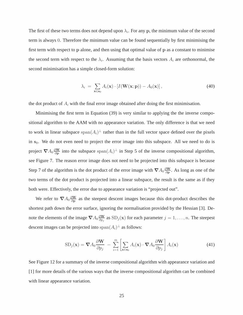
We refer to∇A0∂W

∂pas the steepest descent images because this dot-product describes the

shortest path down the error surface, ignoring the normalisation provided by the Hessian [3]. De-

note the elements of the image∇A0∂W∂pj

asSDj(x) for each parameterj = 1, . . . , n. The steepest

descent images can be projected intospan(Ai)⊥ as follows:

SDj(x) = ∇A0∂W

∂pj

−m

∑

i=1

[

∑

x∈s0

Ai(x) ·∇A0∂W

∂pj

]

Ai(x) (41)

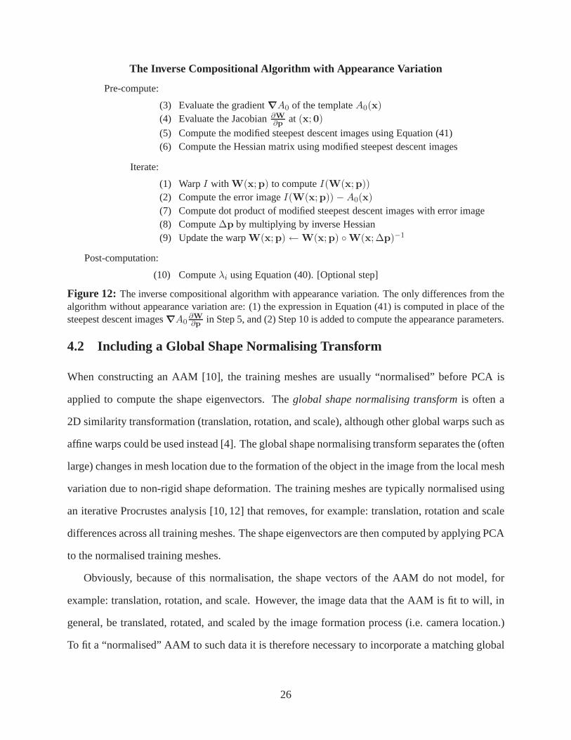
See Figure 12 for a summary of the inverse compositional algorithm with appearance variation and

[1] for more details of the various ways that the inverse compositional algorithm can be combined

with linear appearance variation.

25

The Inverse Compositional Algorithm with Appearance Variation

Pre-compute:

(3) Evaluate the gradient∇A0 of the templateA0(x)

(4) Evaluate the Jacobian∂W∂p

at (x;0)

(5) Compute the modified steepest descent images using Equation (41)(6) Compute the Hessian matrix using modified steepest descent images

Iterate:

(1) WarpI with W(x;p) to computeI(W(x;p))

(2) Compute the error imageI(W(x;p)) −A0(x)

(7) Compute dot product of modified steepest descent images with error image(8) Compute∆p by multiplying by inverse Hessian(9) Update the warpW(x;p)←W(x;p) ◦W(x;∆p)−1

Post-computation:

(10) Computeλi using Equation (40). [Optional step]

Figure 12: The inverse compositional algorithm with appearance variation. The only differences from thealgorithm without appearance variation are: (1) the expression in Equation (41) is computed in place of thesteepest descent images∇A0

∂W∂p

in Step 5, and (2) Step 10 is added to compute the appearance parameters.

4.2 Including a Global Shape Normalising Transform

When constructing an AAM [10], the training meshes are usually “normalised” before PCA is

applied to compute the shape eigenvectors. Theglobal shape normalising transformis often a

2D similarity transformation (translation, rotation, andscale), although other global warps such as

affine warps could be used instead [4]. The global shape normalising transform separates the (often

large) changes in mesh location due to the formation of the object in the image from the local mesh

variation due to non-rigid shape deformation. The trainingmeshes are typically normalised using

an iterative Procrustes analysis [10, 12] that removes, forexample: translation, rotation and scale

differences across all training meshes. The shape eigenvectors are then computed by applying PCA

to the normalised training meshes.

Obviously, because of this normalisation, the shape vectors of the AAM do not model, for

example: translation, rotation, and scale. However, the image data that the AAM is fit to will, in

general, be translated, rotated, and scaled by the image formation process (i.e. camera location.)

To fit a “normalised” AAM to such data it is therefore necessary to incorporate a matching global

26

shape transform to the AAM.

In this section we describe the 2D similarity transform we use for global shape normalisation.

We also show how to parameterize it to simplify computation for the inverse compositional AAM

fitting algorithm that includes a global shape transform.

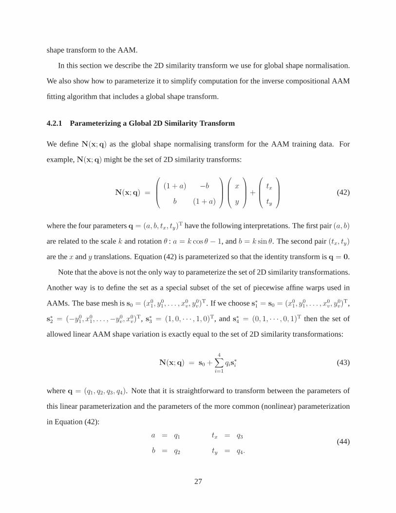
4.2.1 Parameterizing a Global 2D Similarity Transform

We defineN(x;q) as the global shape normalising transform for the AAM training data. For

example,N(x;q) might be the set of 2D similarity transforms:

N(x;q) =

(1 + a) −b

b (1 + a)

x

y

+

tx

ty

(42)

where the four parametersq = (a, b, tx, ty)T have the following interpretations. The first pair(a, b)

are related to the scalek and rotationθ : a = k cos θ − 1, andb = k sin θ. The second pair(tx, ty)

are thex andy translations. Equation (42) is parameterized so that the identity transform isq = 0.

Note that the above is not the only way to parameterize the setof 2D similarity transformations.

Another way is to define the set as a special subset of the set ofpiecewise affine warps used in

AAMs. The base mesh iss0 = (x01, y

01, . . . , x

0v, y

0v)

T. If we chooses∗1 = s0 = (x01, y

01, . . . , x

0v, y

0v)

T,

s∗2 = (−y01, x

01, . . . ,−y0

v , x0v)

T, s∗3 = (1, 0, · · · , 1, 0)T, ands∗4 = (0, 1, · · · , 0, 1)T then the set of

allowed linear AAM shape variation is exactly equal to the set of 2D similarity transformations:

N(x;q) = s0 +4

∑

i=1

qis∗i (43)

whereq = (q1, q2, q3, q4). Note that it is straightforward to transform between the parameters of

this linear parameterization and the parameters of the morecommon (nonlinear) parameterization

in Equation (42):

a = q1 tx = q3

b = q2 ty = q4.(44)

27

We use the representation ofN in Equation (43) because this is similar to that ofW and therefore

much of the analysis in Section 4.1 can be reused, most notably the derivation of the Jacobian.

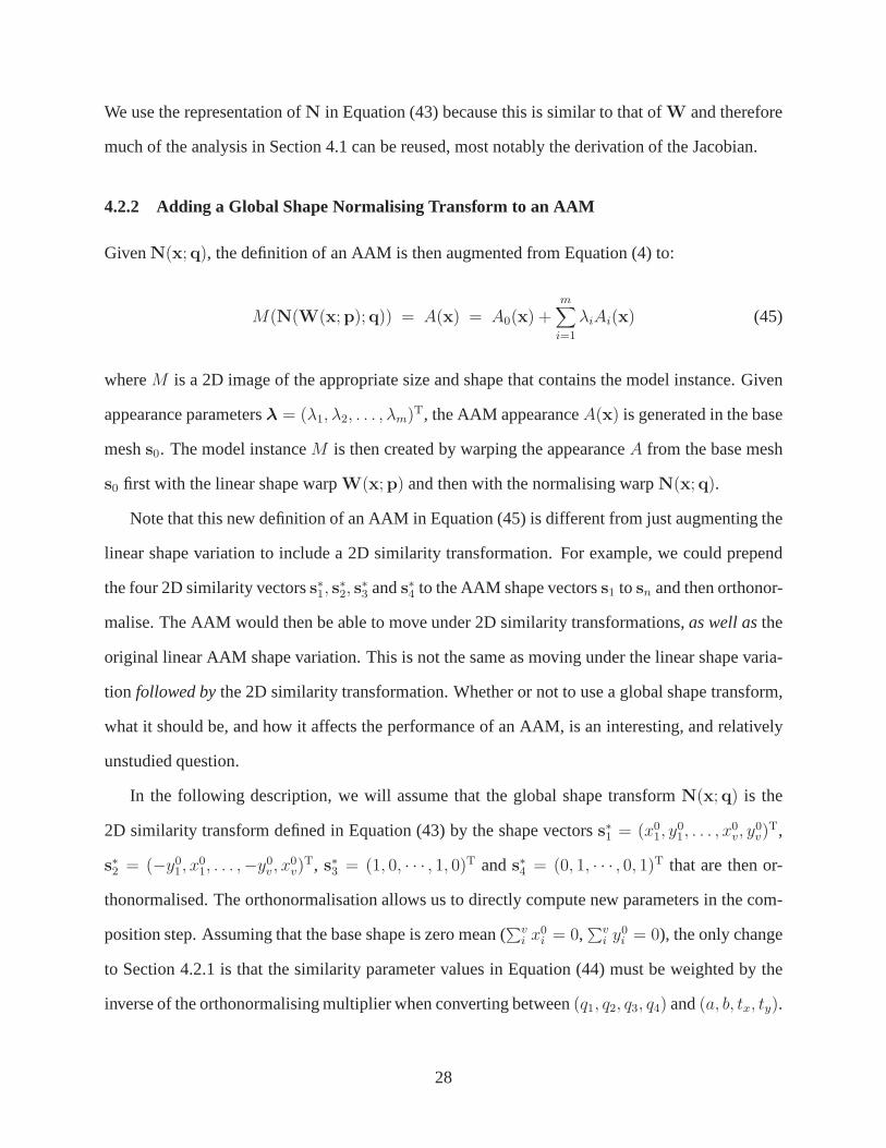
4.2.2 Adding a Global Shape Normalising Transform to an AAM

GivenN(x;q), the definition of an AAM is then augmented from Equation (4) to:

M(N(W(x;p);q)) = A(x) = A0(x) +m

∑

i=1

λiAi(x) (45)

whereM is a 2D image of the appropriate size and shape that contains the model instance. Given

appearance parametersλ = (λ1, λ2, . . . , λm)T, the AAM appearanceA(x) is generated in the base

meshs0. The model instanceM is then created by warping the appearanceA from the base mesh

s0 first with the linear shape warpW(x;p) and then with the normalising warpN(x;q).

Note that this new definition of an AAM in Equation (45) is different from just augmenting the

linear shape variation to include a 2D similarity transformation. For example, we could prepend

the four 2D similarity vectorss∗1, s∗2, s

∗3 ands∗4 to the AAM shape vectorss1 to sn and then orthonor-

malise. The AAM would then be able to move under 2D similaritytransformations,as well asthe

original linear AAM shape variation. This is not the same as moving under the linear shape varia-

tion followed bythe 2D similarity transformation. Whether or not to use a global shape transform,

what it should be, and how it affects the performance of an AAM, is an interesting, and relatively

unstudied question.

In the following description, we will assume that the globalshape transformN(x;q) is the

2D similarity transform defined in Equation (43) by the shapevectorss∗1 = (x01, y

01, . . . , x

0v, y

0v)

T,

s∗2 = (−y01, x

01, . . . ,−y0

v , x0v)

T, s∗3 = (1, 0, · · · , 1, 0)T ands∗4 = (0, 1, · · · , 0, 1)T that are then or-

thonormalised. The orthonormalisation allows us to directly compute new parameters in the com-

position step. Assuming that the base shape is zero mean (∑v

i x0i = 0,

∑vi y0

i = 0), the only change

to Section 4.2.1 is that the similarity parameter values in Equation (44) must be weighted by the

inverse of the orthonormalising multiplier when converting between(q1, q2, q3, q4) and(a, b, tx, ty).

28

Furthermore, we assume that the two sets of shape vectorssi ands∗i are orthogonal to each other.

This should happen automatically when the AAM is constructed. When each shape vector is nor-

malised by removing the similarity transform, we effectively project it into the subspace orthogonal

to s∗i . Since the shape vectorssi are computed by applying PCA to a collection of vectors that are

orthogonal tos∗i , they themselves should be orthogonal tos∗i . In practice, due to various sources

of noise,si and s∗i are never quite orthogonal to each other. This minor error only affects the

composition step and can either be ignored or, preferably, the complete set ofsi ands∗i can be

orthonormalised.

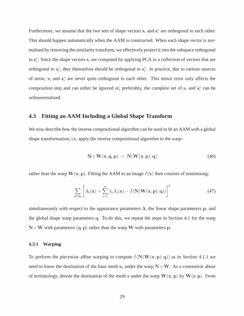
4.3 Fitting an AAM Including a Global Shape Transform

We now describe how the inverse compositional algorithm canbe used to fit an AAM with a global

shape transformation; i.e. apply the inverse compositional algorithm to the warp:

N ◦W(x;q,p) = N(W(x;p);q) (46)

rather than the warpW(x;p). Fitting the AAM to an imageI(x) then consists of minimising:

∑

x∈s0

[

A0(x) +m

∑

i=1

λiAi(x)− I(N(W(x;p);q))

]2

(47)

simultaneously with respect to the appearance parametersλ, the linear shape parametersp, and

the global shape warp parametersq. To do this, we repeat the steps in Section 4.1 for the warp

N ◦W with parameters(q,p) rather than the warpW with parametersp.

4.3.1 Warping

To perform the piecewise affine warping to computeI(N(W(x;p);q)) as in Section 4.1.1 we

need to know the destination of the base meshs0 under the warpN ◦W. As a convenient abuse

of terminology, denote the destination of the meshs under the warpW(x;p) by W(s;p). From

29

Equation (2) we have:

W(s0;p) = s0 +n

∑

i=1

pisi. (48)

We now want to computeN(W(s0;p);q); i.e. we need to warp every vertex inW(s0;p) with the

2D similarity transformN(x;q). This can be performed in the following manner. Since:

N(s0;q) = s0 +4

∑

i=1

qis∗i (49)

we can compute the destination ofs0 underN, and in particular, the destination of any one triangle

underN. Using the technique described in Section 4.1.1 we can compute the affine warp for this

triangle. Since the set of 2D similarity transforms is a subset of the set of affine warps, we can

just apply this affine warp to every vertex inW(s0;p) to compute the destination of the base mesh

underN◦W. The piecewise affine warping is then performed exactly as described in Section 4.1.1.

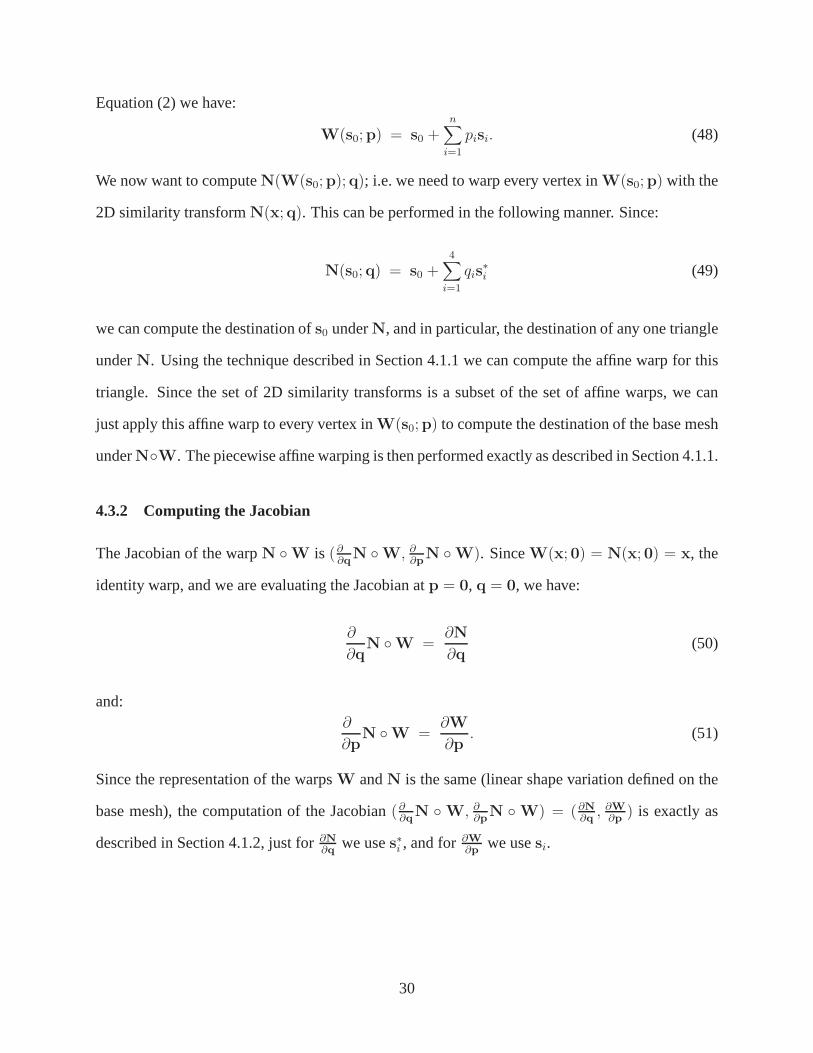
4.3.2 Computing the Jacobian

The Jacobian of the warpN ◦W is (∂∂q

N ◦W, ∂∂p

N ◦W). SinceW(x; 0) = N(x; 0) = x, the

identity warp, and we are evaluating the Jacobian atp = 0, q = 0, we have:

∂

∂qN ◦W =

∂N

∂q(50)

and:∂

∂pN ◦W =

∂W

∂p. (51)

Since the representation of the warpsW andN is the same (linear shape variation defined on the

base mesh), the computation of the Jacobian(∂∂q

N ◦W, ∂∂p

N ◦W) = (∂N∂q

, ∂W∂p

) is exactly as

described in Section 4.1.2, just for∂N∂q

we uses∗i , and for∂W∂p

we usesi.

30

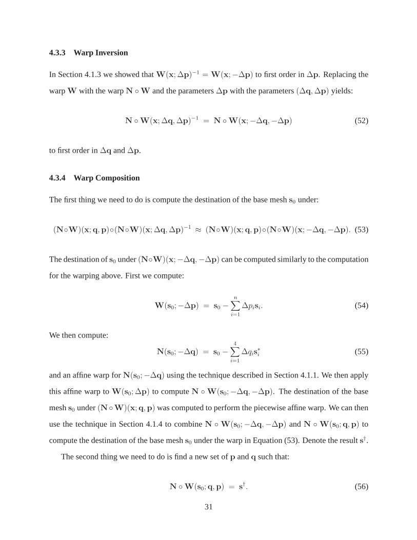
4.3.3 Warp Inversion

In Section 4.1.3 we showed thatW(x; ∆p)−1 = W(x;−∆p) to first order in∆p. Replacing the

warpW with the warpN ◦W and the parameters∆p with the parameters(∆q, ∆p) yields:

N ◦W(x; ∆q, ∆p)−1 = N ◦W(x;−∆q,−∆p) (52)

to first order in∆q and∆p.

4.3.4 Warp Composition

The first thing we need to do is compute the destination of the base meshs0 under:

(N◦W)(x;q,p)◦(N◦W)(x; ∆q, ∆p)−1 ≈ (N◦W)(x;q,p)◦(N◦W)(x;−∆q,−∆p). (53)

The destination ofs0 under(N◦W)(x;−∆q,−∆p) can be computed similarly to the computation

for the warping above. First we compute:

W(s0;−∆p) = s0 −n

∑

i=1

∆pisi. (54)

We then compute:

N(s0;−∆q) = s0 −4

∑

i=1

∆qis∗i (55)

and an affine warp forN(s0;−∆q) using the technique described in Section 4.1.1. We then apply

this affine warp toW(s0; ∆p) to computeN ◦W(s0;−∆q,−∆p). The destination of the base

meshs0 under(N ◦W)(x;q,p) was computed to perform the piecewise affine warp. We can then

use the technique in Section 4.1.4 to combineN ◦W(s0;−∆q,−∆p) andN ◦W(s0;q,p) to

compute the destination of the base meshs0 under the warp in Equation (53). Denote the results†.

The second thing we need to do is find a new set ofp andq such that:

N ◦W(s0;q,p) = s†. (56)

31

In general solving this equation forq andp is a non-linear optimisation. ForN a 2D similarity

transform, however, the problem can be solved fairly easily. First note that:

N ◦W(s0;q,p) = N(s0 +n

∑

i=1

pisi;q). (57)

SinceN can also take the form in Equation (42), this expression equals:

N(s0;q) +

(1 + a) −b

b (1 + a)

n∑

i=1

pisi (58)

where we have again abused the terminology. The multiple of the 2 × 2 matrix with the2v di-

mensional shape vectors is performed by extracting each pair of matchingxy vertex coordinates in

turn, mutliplying by the2× 2 matrix, and then replacing. We can rewrite Equation (58) as:

N(s0;q) +

(1 + a)

1 0

0 1

n∑

i=1

pisi

+

b

0 −1

1 0

n∑

i=1

pisi

. (59)

The second2 term in Equation (59) is orthogonal tos∗i becausesi is orthogonal tos∗i . The third

term in Equation (59) is orthogonal tos∗i because, for every vector ins∗i if we switch the role ofx

andy and change the sign of one of them we still have a vector that is(a constant multiple of) one

of the others∗i .

SinceN(s0;q) = s0 +∑4

i=1 qis∗i we therefore wish to solve:

s0 +4

∑

i=1

qis∗i +

(1 + a)

1 0

0 1

n∑

i=1

pisi

+

b

0 −1

1 0

n∑

i=1

pisi

= s† (60)

the solution of which forqi, using the orthogonality relations discussed above, is:

qi = s∗i · (s† − s0). (61)

2This argument is only applicable to 2D similarity warps. A similar argument may also be possible for affinewarps. For a general global warpN, however, there is likely to be no corresponding derivation.

32

Once the parametersq are known we can then compute:

pi = si · (N(s†;q)−1 − s0). (62)

Note that these last two equations correspond to Equation (36) in Section 4.1.4.

4.3.5 Appearance Variation

The treatment of appearance variation is exactly as in Section 4.1.5. Solving for the warpN ◦W

rather than forW does not change anything except that the steepest descent images for bothp and

q need to be projected intospan(Ai)⊥ using the equivalent of Equation (41).

The inverse compositional AAM fitting algorithm including appearance variation and global

shape transform is summarised in Figure 13. In Step 5 we compute the modified steepest descent

images:

SDj(x) = ∇A0∂N

∂qj

−m

∑

i=1

[

∑

x∈s0

Ai(x) ·∇A0∂N

∂qj

]

Ai(x) (63)

for each of the four normalised similarity parameters(q1, q2, q3, q4) and:

SDj+4(x) = ∇A0∂W

∂pj

−m

∑

i=1

[

∑

x∈s0

Ai(x) ·∇A0∂W

∂pj

]

Ai(x) (64)

for p wherej = 1, . . . , n. The concatenated steepest descent images form a single vector with

four images forq followed byn images forp. If we denote the elements of this vectorSDj(x) for

j = 1, . . . , n + 4, the(j, k)th element of the(n + 4)× (n + 4) Hessian matrix is then computed in

Step 6 as:

Hj,k =∑

x∈s0

SDj(x) · SDk(x). (65)

We compute the appearance parameters in Step (10) using:

λi =∑

x∈s0

Ai(x) · [I(N(W(x;p);q))− A0(x)] . (66)

33

Inverse Compositional Algorithm with Appearance Variation and Global Shape Transform

Pre-compute:

(3) Evaluate the gradient∇A0 of the templateA0(x)

(4) Evaluate the Jacobians∂W∂p

and ∂N∂q

at (x;0)

(5) Compute the modified steepest descent images using Equations (63) and (64)(6) Compute the Hessian matrix using Equation (65)

Iterate:

(1) WarpI with W(x;p) followed byN(x;q) to computeI(N(W(x;p);q))

(2) Compute the error imageI(N(W(x;p);q)) −A0(x)

(7) Compute∑

x∈s0SDi(x) · [I(N(W(x;p);q)) −A0(x)] for i = 1, . . . , n + 4

(8) Compute(∆q,∆p) by multiplying the resulting vector by the inverse Hessian(9) Update(N ◦W)(x;q,p) ← (N ◦W)(x;q,p) ◦ (N ◦W)(x;∆q,∆p)−1

Post-computation:

(10) Computeλi using Equation (66). [Optional step]

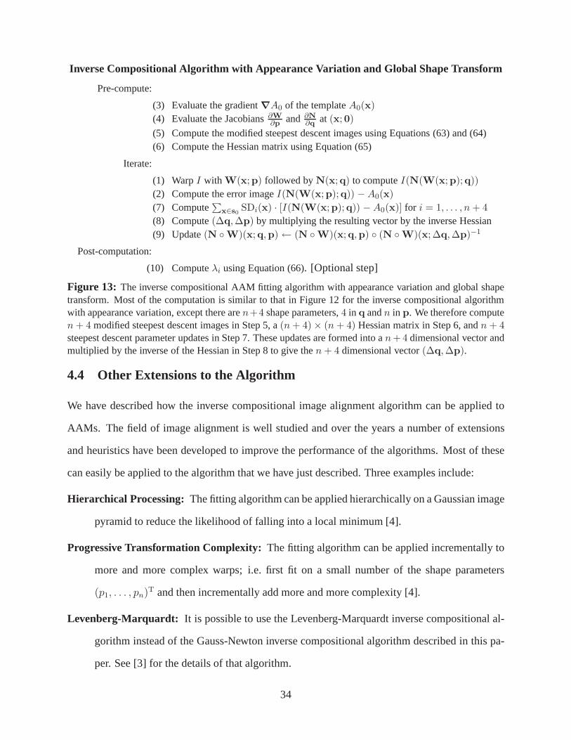
Figure 13: The inverse compositional AAM fitting algorithm with appearance variation and global shapetransform. Most of the computation is similar to that in Figure 12 for the inverse compositional algorithmwith appearance variation, except there aren+4 shape parameters,4 in q andn in p. We therefore computen + 4 modified steepest descent images in Step 5, a(n + 4)× (n + 4) Hessian matrix in Step 6, andn + 4steepest descent parameter updates in Step 7. These updatesare formed into an + 4 dimensional vector andmultiplied by the inverse of the Hessian in Step 8 to give then + 4 dimensional vector(∆q,∆p).

4.4 Other Extensions to the Algorithm

We have described how the inverse compositional image alignment algorithm can be applied to

AAMs. The field of image alignment is well studied and over theyears a number of extensions

and heuristics have been developed to improve the performance of the algorithms. Most of these

can easily be applied to the algorithm that we have just described. Three examples include:

Hierarchical Processing: The fitting algorithm can be applied hierarchically on a Gaussian image

pyramid to reduce the likelihood of falling into a local minimum [4].

Progressive Transformation Complexity: The fitting algorithm can be applied incrementally to

more and more complex warps; i.e. first fit on a small number of the shape parameters

(p1, . . . , pn)T and then incrementally add more and more complexity [4].

Levenberg-Marquardt: It is possible to use the Levenberg-Marquardt inverse compositional al-

gorithm instead of the Gauss-Newton inverse compositionalalgorithm described in this pa-

per. See [3] for the details of that algorithm.

34

5 Empirical Evaluation

We have proposed a new fitting algorithm for AAMs. The performance of AAM fitting algorithms

depends on a wide variety of factors. For example, it dependson whether hierarchical process-

ing, progressive transformation complexity, and adaptivestep-size algorithms such as Levenberg-

Marquardt are used. See Section 4.4. The performance can also be very dependent on minor

details such as the definition of the gradient filter used to compute∇A0. Comparing like with like

is therefore very difficult. Another thing that makes empirical evaluation hard is the wide variety

of AAM fitting algorithms [6,7,11,18,21] and the lack of a standard test set.

In our evaluation we take the following philosophy. Insteadof comparing our algorithm with

the original AAM fitting algorithm or any other algorithm (the results of which would have limited

meaning), we set up a collection of systematic experiments where we only vary one component of

the algorithm. In this paper, we have discussed three main changes to AAM fitting:

1. We use the inverse compositional warp update rather than the additive; i.e. we use Step 9 inFigure 13 to update the warp parameters rather than simply updatingp← p + ∆p.

2. We use an analytical derivation of the steepest descent images rather than a numerical ap-proximation [11,15,21].

3. We project out the appearance variation as described in Section 4.1.5 rather than fitting forit as in [11,15,21].

Each of these changes can be made independently and so we evaluate each one independently. We

compare our AAM fitting algorithm with and without each of these changes. For example, in the

first experiment we try the two alternatives for Step 9 of the algorithm and compare them. Every

other line of code in the implementation is exactly the same.

5.1 Constructing the AAMs

One choice we need to make to test the algorithms is the content of the AAM. There are a wide

variety of applications for AAMs. An AAM could be constructed for a specific person and used

to track that person’s face. Alternatively, a generic AAM could be constructed using images of a

35

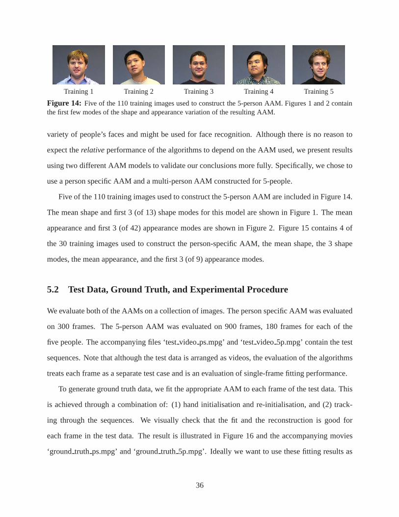
Training 1 Training 2 Training 3 Training 4 Training 5

Figure 14: Five of the 110 training images used to construct the 5-person AAM. Figures 1 and 2 containthe first few modes of the shape and appearance variation of the resulting AAM.

variety of people’s faces and might be used for face recognition. Although there is no reason to

expect therelativeperformance of the algorithms to depend on the AAM used, we present results

using two different AAM models to validate our conclusions more fully. Specifically, we chose to

use a person specific AAM and a multi-person AAM constructed for 5-people.

Five of the 110 training images used to construct the 5-person AAM are included in Figure 14.

The mean shape and first 3 (of 13) shape modes for this model areshown in Figure 1. The mean

appearance and first 3 (of 42) appearance modes are shown in Figure 2. Figure 15 contains 4 of

the 30 training images used to construct the person-specificAAM, the mean shape, the 3 shape

modes, the mean appearance, and the first 3 (of 9) appearance modes.

5.2 Test Data, Ground Truth, and Experimental Procedure

We evaluate both of the AAMs on a collection of images. The person specific AAM was evaluated

on 300 frames. The 5-person AAM was evaluated on 900 frames, 180 frames for each of the

five people. The accompanying files ‘testvideo ps.mpg’ and ‘testvideo 5p.mpg’ contain the test

sequences. Note that although the test data is arranged as videos, the evaluation of the algorithms

treats each frame as a separate test case and is an evaluationof single-frame fitting performance.

To generate ground truth data, we fit the appropriate AAM to each frame of the test data. This

is achieved through a combination of: (1) hand initialisation and re-initialisation, and (2) track-

ing through the sequences. We visually check that the fit and the reconstruction is good for

each frame in the test data. The result is illustrated in Figure 16 and the accompanying movies

‘ground truth ps.mpg’ and ‘groundtruth 5p.mpg’. Ideally we want to use these fitting results as

36

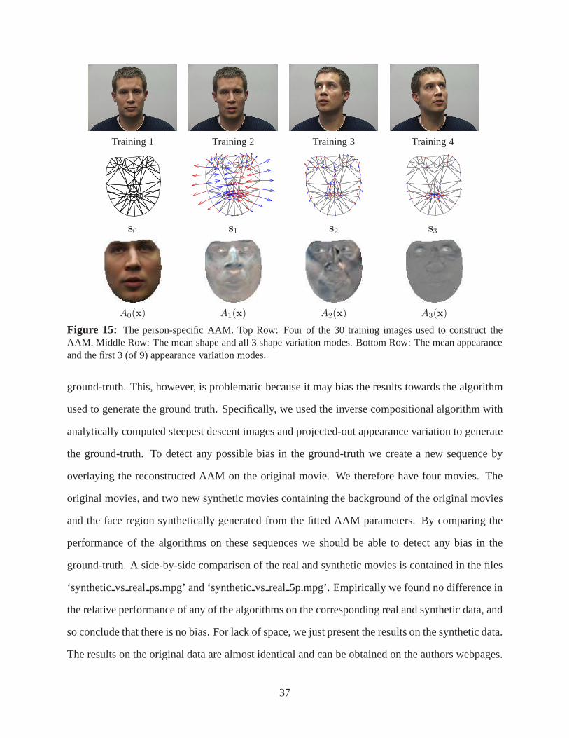
Training 1 Training 2 Training 3 Training 4

s0 s1 s2 s3

A0(x) A1(x) A2(x) A3(x)

Figure 15: The person-specific AAM. Top Row: Four of the 30 training images used to construct theAAM. Middle Row: The mean shape and all 3 shape variation modes. Bottom Row: The mean appearanceand the first 3 (of 9) appearance variation modes.

ground-truth. This, however, is problematic because it maybias the results towards the algorithm

used to generate the ground truth. Specifically, we used the inverse compositional algorithm with

analytically computed steepest descent images and projected-out appearance variation to generate

the ground-truth. To detect any possible bias in the ground-truth we create a new sequence by

overlaying the reconstructed AAM on the original movie. We therefore have four movies. The

original movies, and two new synthetic movies containing the background of the original movies

and the face region synthetically generated from the fitted AAM parameters. By comparing the

performance of the algorithms on these sequences we should be able to detect any bias in the

ground-truth. A side-by-side comparison of the real and synthetic movies is contained in the files

‘syntheticvs real ps.mpg’ and ‘syntheticvs real 5p.mpg’. Empirically we found no difference in

the relative performance of any of the algorithms on the corresponding real and synthetic data, and

so conclude that there is no bias. For lack of space, we just present the results on the synthetic data.

The results on the original data are almost identical and canbe obtained on the authors webpages.

37

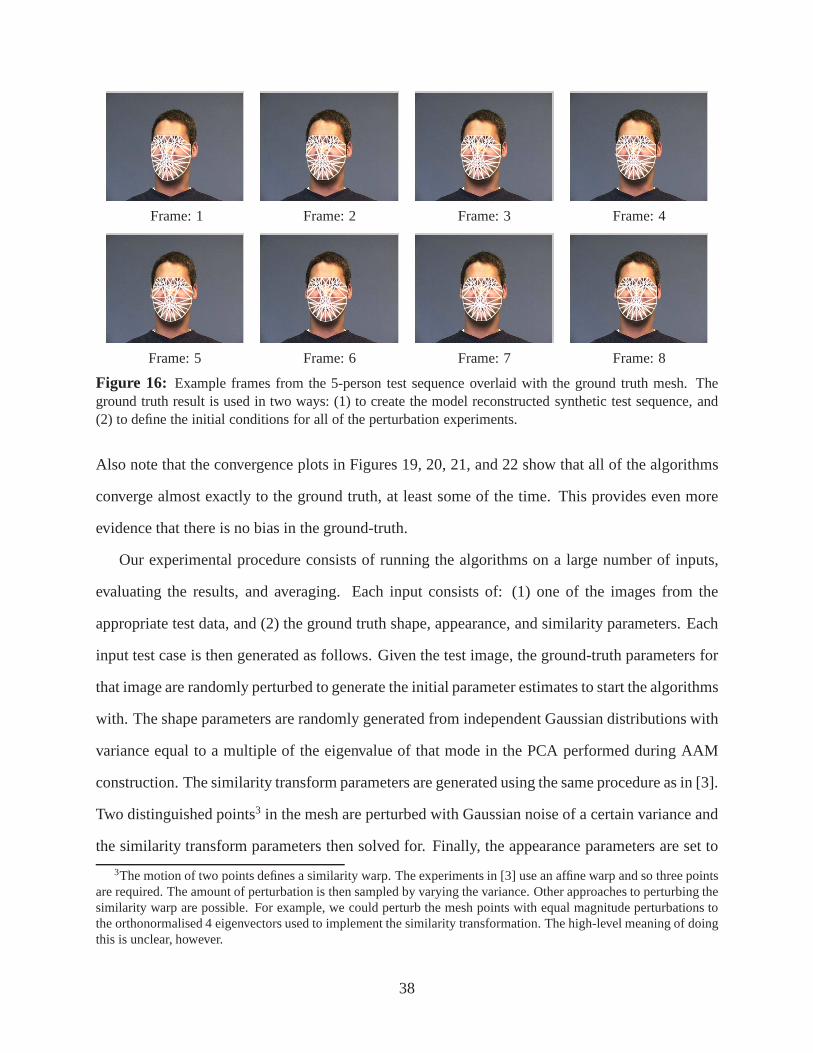
Frame: 1 Frame: 2 Frame: 3 Frame: 4

Frame: 5 Frame: 6 Frame: 7 Frame: 8

Figure 16: Example frames from the 5-person test sequence overlaid with the ground truth mesh. Theground truth result is used in two ways: (1) to create the model reconstructed synthetic test sequence, and(2) to define the initial conditions for all of the perturbation experiments.

Also note that the convergence plots in Figures 19, 20, 21, and 22 show that all of the algorithms

converge almost exactly to the ground truth, at least some ofthe time. This provides even more

evidence that there is no bias in the ground-truth.

Our experimental procedure consists of running the algorithms on a large number of inputs,

evaluating the results, and averaging. Each input consistsof: (1) one of the images from the

appropriate test data, and (2) the ground truth shape, appearance, and similarity parameters. Each

input test case is then generated as follows. Given the test image, the ground-truth parameters for

that image are randomly perturbed to generate the initial parameter estimates to start the algorithms

with. The shape parameters are randomly generated from independent Gaussian distributions with

variance equal to a multiple of the eigenvalue of that mode inthe PCA performed during AAM

construction. The similarity transform parameters are generated using the same procedure as in [3].

Two distinguished points3 in the mesh are perturbed with Gaussian noise of a certain variance and

the similarity transform parameters then solved for. Finally, the appearance parameters are set to

3The motion of two points defines a similarity warp. The experiments in [3] use an affine warp and so three pointsare required. The amount of perturbation is then sampled by varying the variance. Other approaches to perturbing thesimilarity warp are possible. For example, we could perturbthe mesh points with equal magnitude perturbations tothe orthonormalised 4 eigenvectors used to implement the similarity transformation. The high-level meaning of doingthis is unclear, however.

38

be the mean appearance.

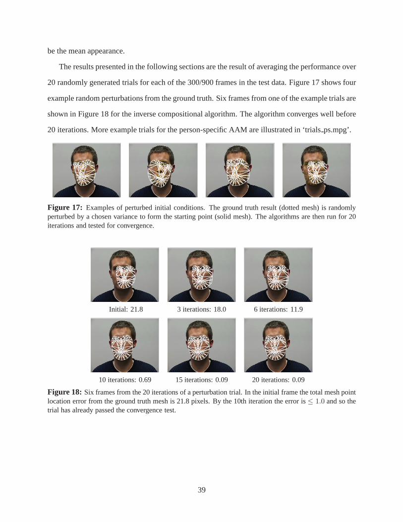
The results presented in the following sections are the result of averaging the performance over

20 randomly generated trials for each of the 300/900 frames in the test data. Figure 17 shows four

example random perturbations from the ground truth. Six frames from one of the example trials are

shown in Figure 18 for the inverse compositional algorithm.The algorithm converges well before

20 iterations. More example trials for the person-specific AAM are illustrated in ‘trialsps.mpg’.

Figure 17: Examples of perturbed initial conditions. The ground truthresult (dotted mesh) is randomlyperturbed by a chosen variance to form the starting point (solid mesh). The algorithms are then run for 20iterations and tested for convergence.

Initial: 21.8 3 iterations: 18.0 6 iterations: 11.9

10 iterations: 0.69 15 iterations: 0.09 20 iterations: 0.09

Figure 18: Six frames from the 20 iterations of a perturbation trial. Inthe initial frame the total mesh pointlocation error from the ground truth mesh is 21.8 pixels. By the 10th iteration the error is≤ 1.0 and so thetrial has already passed the convergence test.

39

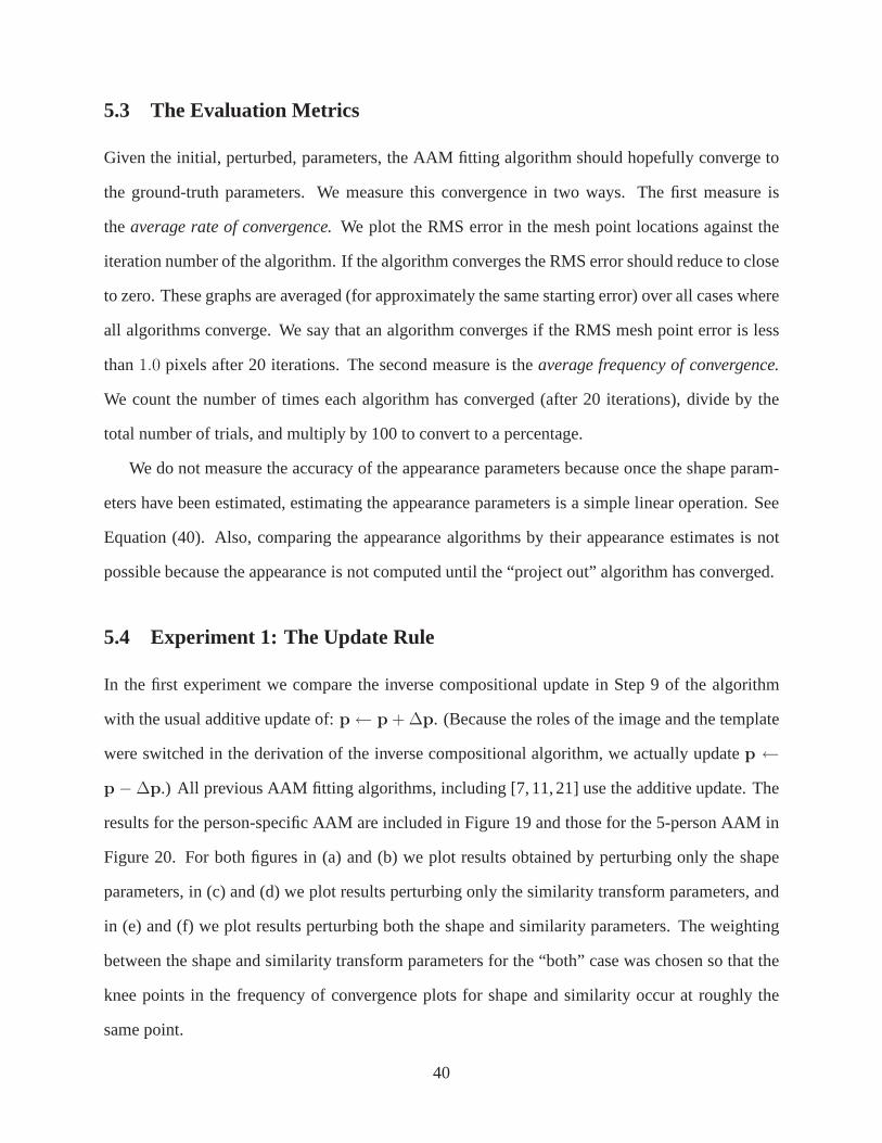
5.3 The Evaluation Metrics

Given the initial, perturbed, parameters, the AAM fitting algorithm should hopefully converge to

the ground-truth parameters. We measure this convergence in two ways. The first measure is

the average rate of convergence.We plot the RMS error in the mesh point locations against the

iteration number of the algorithm. If the algorithm converges the RMS error should reduce to close

to zero. These graphs are averaged (for approximately the same starting error) over all cases where

all algorithms converge. We say that an algorithm convergesif the RMS mesh point error is less

than1.0 pixels after 20 iterations. The second measure is theaverage frequency of convergence.

We count the number of times each algorithm has converged (after 20 iterations), divide by the

total number of trials, and multiply by 100 to convert to a percentage.

We do not measure the accuracy of the appearance parameters because once the shape param-

eters have been estimated, estimating the appearance parameters is a simple linear operation. See

Equation (40). Also, comparing the appearance algorithms by their appearance estimates is not

possible because the appearance is not computed until the “project out” algorithm has converged.

5.4 Experiment 1: The Update Rule

In the first experiment we compare the inverse compositionalupdate in Step 9 of the algorithm

with the usual additive update of:p← p + ∆p. (Because the roles of the image and the template

were switched in the derivation of the inverse compositional algorithm, we actually updatep ←

p −∆p.) All previous AAM fitting algorithms, including [7, 11, 21]use the additive update. The

results for the person-specific AAM are included in Figure 19and those for the 5-person AAM in

Figure 20. For both figures in (a) and (b) we plot results obtained by perturbing only the shape

parameters, in (c) and (d) we plot results perturbing only the similarity transform parameters, and

in (e) and (f) we plot results perturbing both the shape and similarity parameters. The weighting

between the shape and similarity transform parameters for the “both” case was chosen so that the

knee points in the frequency of convergence plots for shape and similarity occur at roughly the

same point.

40

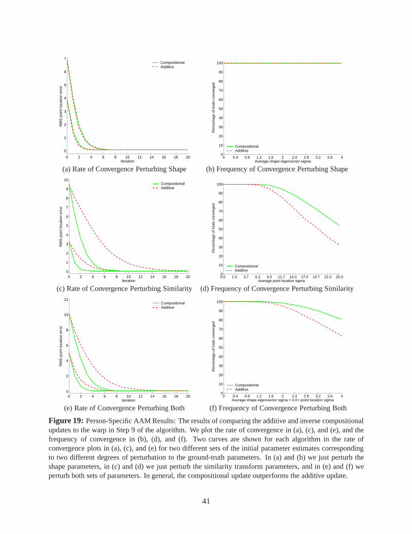
0 2 4 6 8 10 12 14 16 18 20

0

1

2

3

4

5

6

7

Iteration

RM

S p

oint

loca

tion

erro

rCompositionalAdditive

0 0.4 0.8 1.2 1.6 2 2.4 2.8 3.2 3.6 40

10

20

30

40

50

60

70

80

90

100

Per

cent

age

of tr

ials

con

verg

ed

Average shape eigenvector sigma

CompositionalAdditive

(a) Rate of Convergence Perturbing Shape (b) Frequency of Convergence Perturbing Shape

0 2 4 6 8 10 12 14 16 18 200

1

2

3

4

5

6

7

8

9

10

Iteration

RM

S p

oint

loca

tion

erro

r

CompositionalAdditive

0.0 1.0 3.7 6.3 9.0 11.7 14.3 17.0 19.7 22.3 25.00

10

20

30

40

50

60

70

80

90

100

Per

cent

age

of tr

ials

con

verg

ed

Average point location sigma

CompositionalAdditive

(c) Rate of Convergence Perturbing Similarity (d) Frequency of Convergence Perturbing Similarity

0 2 4 6 8 10 12 14 16 18 200

2

4

6

8

10

12

Iteration

RM

S p

oint

loca

tion

erro

r

CompositionalAdditive

0 0.4 0.8 1.2 1.6 2 2.4 2.8 3.2 3.6 40

10

20

30

40

50

60

70

80

90

100

Per

cent

age

of tr

ials

con

verg

ed

Average shape eigenvector sigma + 4.0 × point location sigma

CompositionalAdditive

(e) Rate of Convergence Perturbing Both (f) Frequency of Convergence Perturbing Both

Figure 19: Person-Specific AAM Results: The results of comparing the additive and inverse compositionalupdates to the warp in Step 9 of the algorithm. We plot the rateof convergence in (a), (c), and (e), and thefrequency of convergence in (b), (d), and (f). Two curves areshown for each algorithm in the rate ofconvergence plots in (a), (c), and (e) for two different setsof the initial parameter estimates correspondingto two different degrees of perturbation to the ground-truth parameters. In (a) and (b) we just perturb theshape parameters, in (c) and (d) we just perturb the similarity transform parameters, and in (e) and (f) weperturb both sets of parameters. In general, the compositional update outperforms the additive update.

41

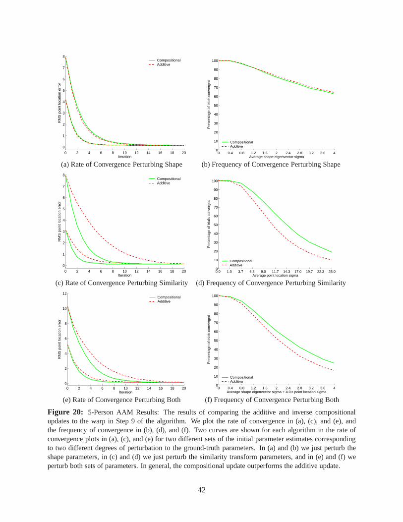
0 2 4 6 8 10 12 14 16 18 20

0

1

2

3

4

5

6

7

8

Iteration

RM

S p

oint

loca

tion

erro

rCompositionalAdditive

0 0.4 0.8 1.2 1.6 2 2.4 2.8 3.2 3.6 40

10

20

30

40

50

60

70

80

90

100

Per

cent

age

of tr

ials

con

verg

ed

Average shape eigenvector sigma

CompositionalAdditive

(a) Rate of Convergence Perturbing Shape (b) Frequency of Convergence Perturbing Shape

0 2 4 6 8 10 12 14 16 18 20

0

1

2

3

4

5

6

7

8

Iteration

RM

S p

oint

loca

tion

erro

r

CompositionalAdditive

0.0 1.0 3.7 6.3 9.0 11.7 14.3 17.0 19.7 22.3 25.00

10

20

30

40

50

60

70

80

90

100

Per

cent

age

of tr

ials

con

verg

ed

Average point location sigma

CompositionalAdditive

(c) Rate of Convergence Perturbing Similarity (d) Frequency of Convergence Perturbing Similarity

0 2 4 6 8 10 12 14 16 18 200

2

4

6

8

10

12

Iteration

RM

S p

oint

loca

tion

erro

r

CompositionalAdditive

0 0.4 0.8 1.2 1.6 2 2.4 2.8 3.2 3.6 40

10

20

30

40

50

60

70

80

90

100

Per

cent

age

of tr

ials

con

verg

ed

Average shape eigenvector sigma + 4.0 × point location sigma

CompositionalAdditive

(e) Rate of Convergence Perturbing Both (f) Frequency of Convergence Perturbing Both

Figure 20: 5-Person AAM Results: The results of comparing the additiveand inverse compositionalupdates to the warp in Step 9 of the algorithm. We plot the rateof convergence in (a), (c), and (e), andthe frequency of convergence in (b), (d), and (f). Two curvesare shown for each algorithm in the rate ofconvergence plots in (a), (c), and (e) for two different setsof the initial parameter estimates correspondingto two different degrees of perturbation to the ground-truth parameters. In (a) and (b) we just perturb theshape parameters, in (c) and (d) we just perturb the similarity transform parameters, and in (e) and (f) weperturb both sets of parameters. In general, the compositional update outperforms the additive update.

42

The first thing to notice in Figures 19 and 20 is that in most cases the inverse compositional

update outperforms the additive. The rate of convergence isfaster and the frequency of conver-

gence is higher. The one exception is for perturbing only theshape component in (a) and (b). In

this case, the global similarity transform hides the problem described in Section 2.3.3 and so the

addition and inverse composition updates perform very similarly. When the normalising similarity

transformation is used, the shape variation is very small relative to the mesh. The additive update is

therefore a reasonable approximation for the shape parameters. The constant linear update approx-

imation problem is clear for the similarity transform parameters in (c) and (d), and the combined

performance for perturbing both shape and similarity in (e)and (f) is also poor.

Comparing Figures 19 and 20 it is clear that the performance for the person-specific AAM is

far better than the performance for the 5-person AAM. This isexpected because of the greater

shape and appearance variation in the 5-person AAM. Note however, that the relative performance

of the algorithms is the same in both cases.

In the following experiments we only show results for perturbing both shape and similarity

transform parameters. In all cases the “both” results are representative of those obtained for per-

turbing shape or similarity transform parameters alone.

5.5 Experiment 2: Computation of the Steepest Descent Images

The inverse compositional algorithm uses thesteepest descent images∇A0∂W∂p

. The analytically

derived steepest descent images play exactly the same role as the numerically estimated images∂r∂p

in [11] (and the corresponding finite difference images in [15, 21].) The difference between these

two sets of images is that in the additive formulation, the steepest descent images are a function

of p whereas in the inverse compositional formulation they are provably constant. Otherwise their

roles and meaning are identical.

Is it better to analytically compute or numerically estimate the steepest descent images? To

answer this question, we apply the same inverse compositional algorithm using both approaches,

the analytically derived∇A0∂W

∂p, and the numerically estimated∂r

∂pcomputed as described in [11].

43

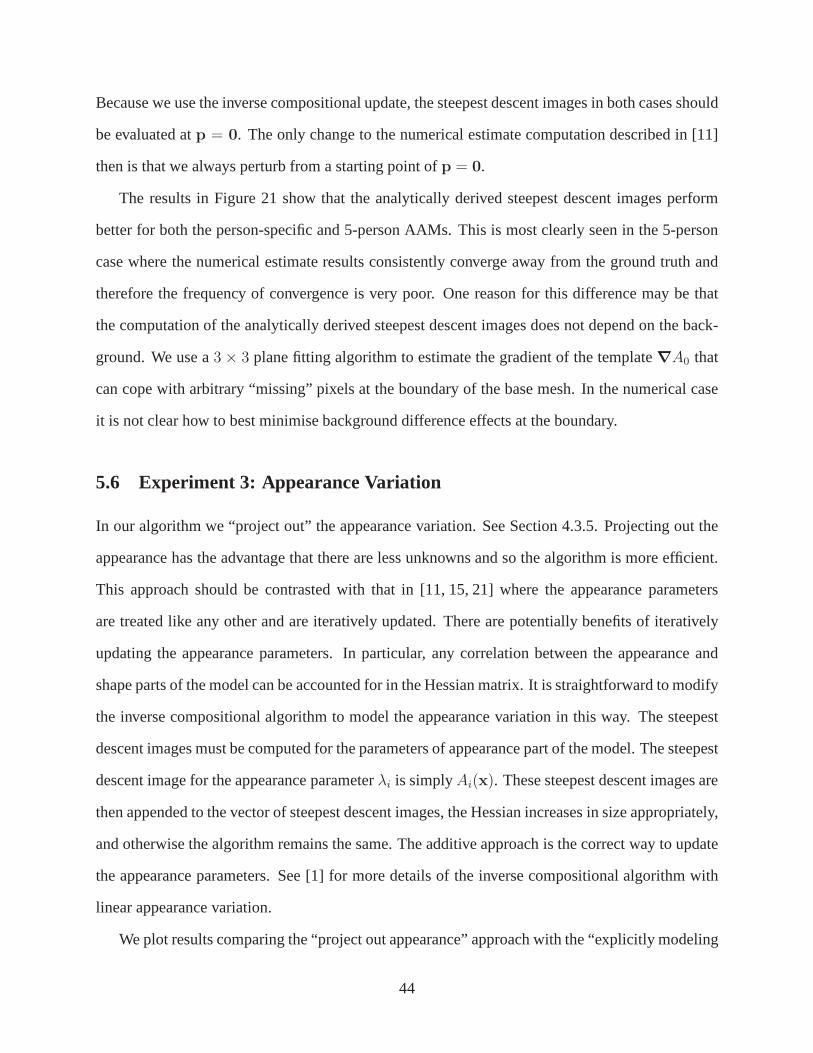
Because we use the inverse compositional update, the steepest descent images in both cases should

be evaluated atp = 0. The only change to the numerical estimate computation described in [11]

then is that we always perturb from a starting point ofp = 0.

The results in Figure 21 show that the analytically derived steepest descent images perform

better for both the person-specific and 5-person AAMs. This is most clearly seen in the 5-person

case where the numerical estimate results consistently converge away from the ground truth and

therefore the frequency of convergence is very poor. One reason for this difference may be that

the computation of the analytically derived steepest descent images does not depend on the back-

ground. We use a3 × 3 plane fitting algorithm to estimate the gradient of the template∇A0 that

can cope with arbitrary “missing” pixels at the boundary of the base mesh. In the numerical case

it is not clear how to best minimise background difference effects at the boundary.

5.6 Experiment 3: Appearance Variation

In our algorithm we “project out” the appearance variation.See Section 4.3.5. Projecting out the

appearance has the advantage that there are less unknowns and so the algorithm is more efficient.

This approach should be contrasted with that in [11, 15, 21] where the appearance parameters

are treated like any other and are iteratively updated. There are potentially benefits of iteratively

updating the appearance parameters. In particular, any correlation between the appearance and

shape parts of the model can be accounted for in the Hessian matrix. It is straightforward to modify

the inverse compositional algorithm to model the appearance variation in this way. The steepest

descent images must be computed for the parameters of appearance part of the model. The steepest

descent image for the appearance parameterλi is simplyAi(x). These steepest descent images are

then appended to the vector of steepest descent images, the Hessian increases in size appropriately,

and otherwise the algorithm remains the same. The additive approach is the correct way to update

the appearance parameters. See [1] for more details of the inverse compositional algorithm with

linear appearance variation.

We plot results comparing the “project out appearance” approach with the “explicitly modeling

44

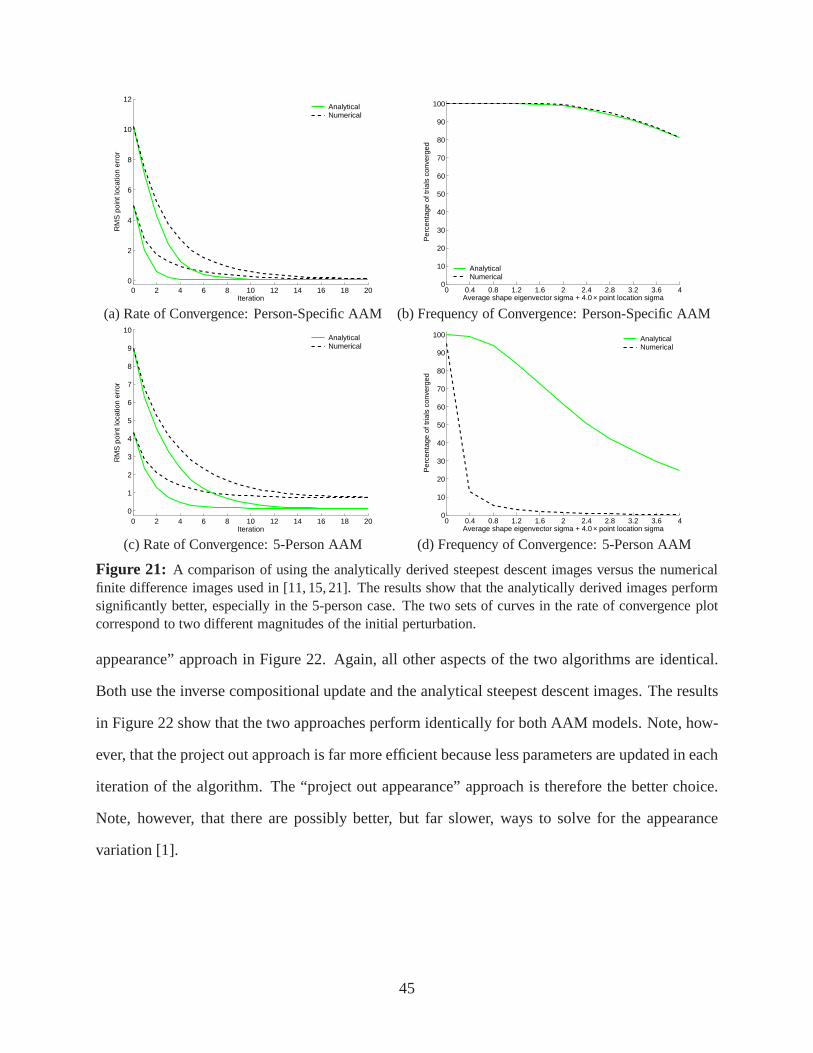
0 2 4 6 8 10 12 14 16 18 200

2

4

6

8

10

12

Iteration

RM

S p

oint

loca

tion

erro

rAnalyticalNumerical

0 0.4 0.8 1.2 1.6 2 2.4 2.8 3.2 3.6 40

10

20

30

40

50

60

70

80

90

100

Per

cent

age

of tr

ials

con

verg

ed

Average shape eigenvector sigma + 4.0 × point location sigma

AnalyticalNumerical

(a) Rate of Convergence: Person-Specific AAM (b) Frequency of Convergence: Person-Specific AAM

0 2 4 6 8 10 12 14 16 18 200

1

2

3

4

5

6

7

8

9

10

Iteration

RM

S p

oint

loca

tion

erro

r

AnalyticalNumerical

0 0.4 0.8 1.2 1.6 2 2.4 2.8 3.2 3.6 40

10

20

30

40

50

60

70

80

90

100

Per

cent

age

of tr

ials

con

verg

ed

Average shape eigenvector sigma + 4.0 × point location sigma

AnalyticalNumerical

(c) Rate of Convergence: 5-Person AAM (d) Frequency of Convergence: 5-Person AAM

Figure 21: A comparison of using the analytically derived steepest descent images versus the numericalfinite difference images used in [11, 15, 21]. The results show that the analytically derived images performsignificantly better, especially in the 5-person case. The two sets of curves in the rate of convergence plotcorrespond to two different magnitudes of the initial perturbation.

appearance” approach in Figure 22. Again, all other aspectsof the two algorithms are identical.

Both use the inverse compositional update and the analytical steepest descent images. The results

in Figure 22 show that the two approaches perform identically for both AAM models. Note, how-

ever, that the project out approach is far more efficient because less parameters are updated in each

iteration of the algorithm. The “project out appearance” approach is therefore the better choice.

Note, however, that there are possibly better, but far slower, ways to solve for the appearance

variation [1].

45

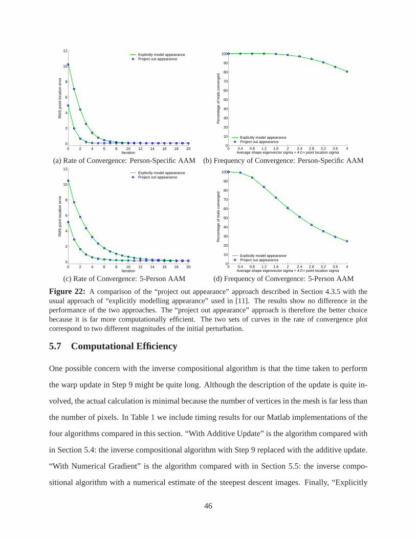
0 2 4 6 8 10 12 14 16 18 200

2

4

6

8

10

12

Iteration

RM

S p

oint

loca

tion

erro

rExplicitly model appearanceProject out appearance

0 0.4 0.8 1.2 1.6 2 2.4 2.8 3.2 3.6 40

10

20

30

40

50

60

70

80

90

100

Per

cent

age

of tr

ials

con

verg

ed

Average shape eigenvector sigma + 4.0 × point location sigma

Explicitly model appearanceProject out appearance

(a) Rate of Convergence: Person-Specific AAM (b) Frequency of Convergence: Person-Specific AAM

0 2 4 6 8 10 12 14 16 18 200

2

4

6

8

10

12

Iteration

RM

S p

oint

loca

tion

erro

r

Explicitly model appearanceProject out appearance

0 0.4 0.8 1.2 1.6 2 2.4 2.8 3.2 3.6 40

10

20

30

40

50

60

70

80

90

100

Per

cent

age

of tr

ials

con

verg

ed

Average shape eigenvector sigma + 4.0 × point location sigma

Explicitly model appearanceProject out appearance

(c) Rate of Convergence: 5-Person AAM (d) Frequency of Convergence: 5-Person AAM

Figure 22: A comparison of the “project out appearance” approach described in Section 4.3.5 with theusual approach of “explicitly modelling appearance” used in [11]. The results show no difference in theperformance of the two approaches. The “project out appearance” approach is therefore the better choicebecause it is far more computationally efficient. The two sets of curves in the rate of convergence plotcorrespond to two different magnitudes of the initial perturbation.

5.7 Computational Efficiency

One possible concern with the inverse compositional algorithm is that the time taken to perform

the warp update in Step 9 might be quite long. Although the description of the update is quite in-

volved, the actual calculation is minimal because the number of vertices in the mesh is far less than

the number of pixels. In Table 1 we include timing results forour Matlab implementations of the

four algorithms compared in this section. “With Additive Update” is the algorithm compared with

in Section 5.4: the inverse compositional algorithm with Step 9 replaced with the additive update.

“With Numerical Gradient” is the algorithm compared with inSection 5.5: the inverse compo-

sitional algorithm with a numerical estimate of the steepest descent images. Finally, “Explicitly

46

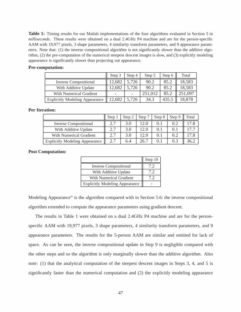
Table 1: Timing results for our Matlab implementations of the four algorithms evaluated in Section 5 inmilliseconds. These results were obtained on a dual 2.4GHz P4 machine and are for the person-specificAAM with 19,977 pixels, 3 shape parameters, 4 similarity transform parameters, and 9 appearance param-eters. Note that: (1) the inverse compositional algorithm is not significantly slower than the additive algo-rithm, (2) the pre-computation of the numerical steepest descent images is slow, and (3) explicitly modelingappearance is significantly slower than projecting out appearance.

Pre-computation:

Step 3 Step 4 Step 5 Step 6 Total

Inverse Compositional 12,682 5,726 90.2 85.2 18,583With Additive Update 12,682 5,726 90.2 85.2 18,583

With Numerical Gradient - - 251,012 85.2 251,097Explicitly Modeling Appearance 12,682 5,726 34.3 435.5 18,878

Per Iteration:

Step 1 Step 2 Step 7 Step 8 Step 9 Total

Inverse Compositional 2.7 3.0 12.0 0.1 0.2 17.8With Additive Update 2.7 3.0 12.0 0.1 0.1 17.7

With Numerical Gradient 2.7 3.0 12.0 0.1 0.2 17.8Explicitly Modeling Appearance 2.7 6.4 26.7 0.1 0.3 36.2

Post Computation:

Step 10

Inverse Compositional 7.2With Additive Update 7.2

With Numerical Gradient 7.2Explicitly Modeling Appearance -

Modeling Appearance” is the algorithm compared with in Section 5.6: the inverse compositional

algorithm extended to compute the appearance parameters using gradient descent.

The results in Table 1 were obtained on a dual 2.4GHz P4 machine and are for the person-

specific AAM with 19,977 pixels, 3 shape parameters, 4 similarity transform parameters, and 9

appearance parameters. The results for the 5-person AAM aresimilar and omitted for lack of

space. As can be seen, the inverse compositional update in Step 9 is negligible compared with

the other steps and so the algorithm is only marginally slower than the additive algorithm. Also

note: (1) that the analytical computation of the steepest descent images in Steps 3, 4, and 5 is

significantly faster than the numerical computation and (2)the explicitly modeling appearance

47

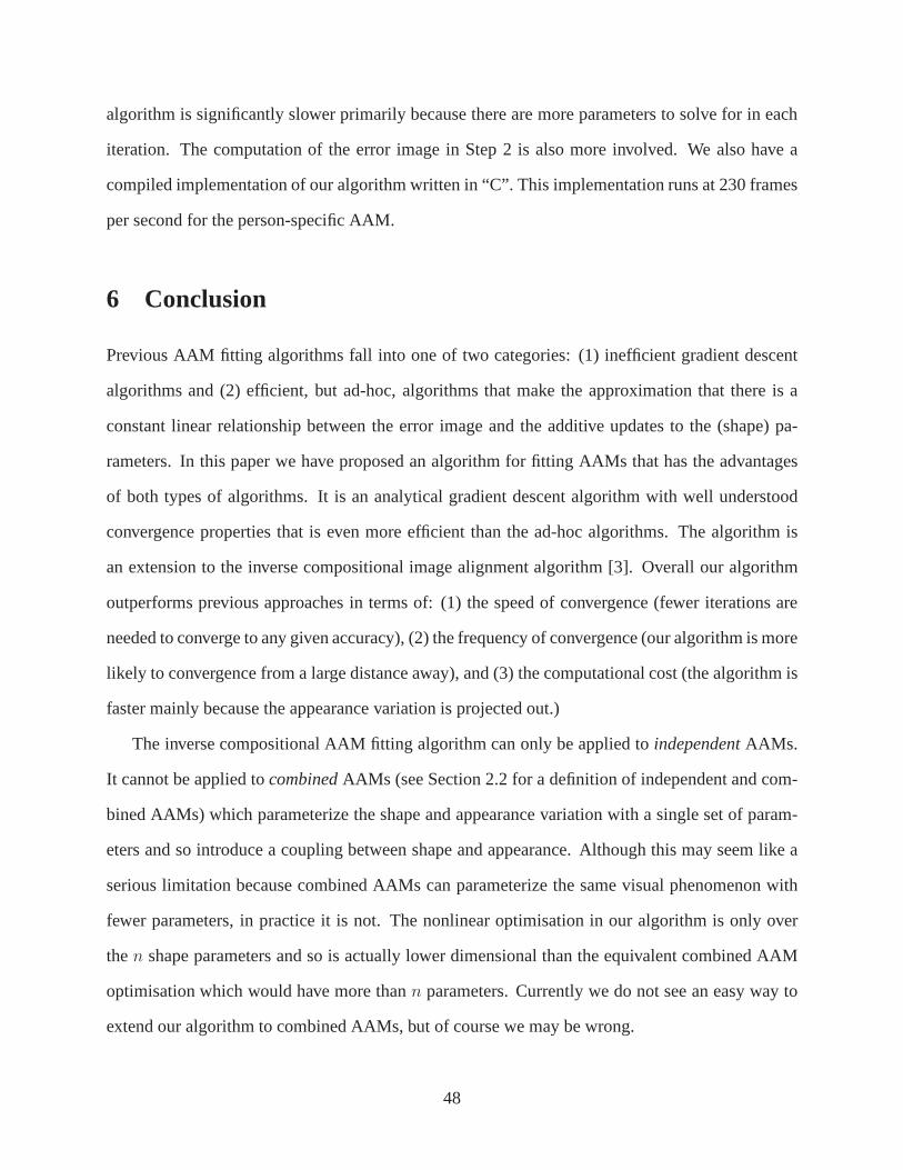
algorithm is significantly slower primarily because there are more parameters to solve for in each

iteration. The computation of the error image in Step 2 is also more involved. We also have a

compiled implementation of our algorithm written in “C”. This implementation runs at 230 frames

per second for the person-specific AAM.

6 Conclusion

Previous AAM fitting algorithms fall into one of two categories: (1) inefficient gradient descent

algorithms and (2) efficient, but ad-hoc, algorithms that make the approximation that there is a

constant linear relationship between the error image and the additive updates to the (shape) pa-

rameters. In this paper we have proposed an algorithm for fitting AAMs that has the advantages

of both types of algorithms. It is an analytical gradient descent algorithm with well understood

convergence properties that is even more efficient than the ad-hoc algorithms. The algorithm is

an extension to the inverse compositional image alignment algorithm [3]. Overall our algorithm

outperforms previous approaches in terms of: (1) the speed of convergence (fewer iterations are

needed to converge to any given accuracy), (2) the frequencyof convergence (our algorithm is more

likely to convergence from a large distance away), and (3) the computational cost (the algorithm is

faster mainly because the appearance variation is projected out.)

The inverse compositional AAM fitting algorithm can only be applied toindependentAAMs.

It cannot be applied tocombinedAAMs (see Section 2.2 for a definition of independent and com-

bined AAMs) which parameterize the shape and appearance variation with a single set of param-

eters and so introduce a coupling between shape and appearance. Although this may seem like a

serious limitation because combined AAMs can parameterizethe same visual phenomenon with

fewer parameters, in practice it is not. The nonlinear optimisation in our algorithm is only over

then shape parameters and so is actually lower dimensional than the equivalent combined AAM

optimisation which would have more thann parameters. Currently we do not see an easy way to

extend our algorithm to combined AAMs, but of course we may bewrong.

48

The inverse compositional algorithm is an image alignment algorithm. Hence most standard

extensions to image alignment can be applied with this algorithm. See Section 4.4. For other

extensions, such as the use of robust norms [5, 16, 21], the situation is not quite so clear. For

example, when a robust norm is used, the orthogonal decomposition of the norm in Equation (38)

is not applicable. The efficient treatment of appearance is therefore more complex [1].

Acknowledgments

We thank Tim Cootes for discussions on the incorporation of the global shape transformation in

Section 4.3. Elements of the AAM fitting algorithm appeared in [2]. We thank the reviewers

of [2] and this IJCV paper for their feedback. The research described in this paper was conducted

under U.S. Office of Naval Research contract N00014-00-1-0915. Additional support was provided

through U.S. Department of Defense award N41756-03-C4024.

References

[1] S. Baker, R. Gross, and I. Matthews. Lucas-Kanade 20 years on: A unifying framework:Part 3. Technical Report CMU-RI-TR-03-35, Carnegie MellonUniversity Robotics Institute,2003.

[2] S. Baker and I. Matthews. Equivalence and efficiency of image alignment algorithms. InProceedings of the IEEE Conference on Computer Vision and Pattern Recognition, volume 1,pages 1090–1097, 2001.

[3] S. Baker and I. Matthews. Lucas-Kanade 20 years on: A unifying framework. Interna-tional Journal of Computer Vision, 56(3):221–255, Feb. 2004. Previously appeared as CMURobotics Institute Technical Report CMU-RI-TR-02-16.

[4] J. Bergen, P. Anandan, K. Hanna, and R. Hingorani. Hierarchical model-based motion es-timation. InProceedings of the European Conference on Computer Vision, pages 237–252,1992.

[5] M. Black and A. Jepson. Eigen-tracking: Robust matchingand tracking of articulated objectsusing a view-based representation.International Journal of Computer Vision, 36(2):101–130,1998.

[6] V. Blanz and T. Vetter. A morphable model for the synthesis of 3D faces. InComputerGraphics, Annual Conference Series (SIGGRAPH), pages 187–194, 1999.

49

[7] T. Cootes, G. Edwards, and C. Taylor. Active appearance models. InProceedings of theEuropean Conference on Computer Vision, volume 2, pages 484–498, 1998.

[8] T. Cootes, G. Edwards, and C. Taylor. A comparitive evaluation of active appearance modelsalgorithms. InProceedings of the British Machine Vision Conference, 1998.

[9] T. Cootes and P. Kittipanya-ngam. Comparing variationson the active appearance modelalgorithm. InProceedings of the British Machine Vision Conference, volume 2, pages 837–846, 2002.

[10] T. F. Cootes. Statistical models of appearance for computer vision. Online technical reportavailable from http://www.isbe.man.ac.uk/˜bim/refs.html, Sept. 2001.

[11] T. F. Cootes, G. J. Edwards, and C. J. Taylor. Active appearance models.IEEE Transactionson Pattern Analysis and Machine Intelligence, 23(6):681–685, June 2001.

[12] I. L. Dryden and K. V. Mardia.Statistical Shape Analysis. Wiley, 1998.

[13] G. J. Edwards.Learning to Identify Faces in Images and Video Sequences. PhD thesis,University of Manchester, Division of Imaging Science and Biomedical Engineering, 1999.

[14] G. J. Edwards, C. J. Taylor, and T. F. Cootes. Interpreting face images using active appearancemodels. InProc. International Conference on Automatic Face and Gesture Recognition,pages 300–305, June 1998.

[15] M. Gleicher. Projective registration with differencedecomposition. InProc. of the IEEEConference on Computer Vision and Pattern Recognition, pages 331–337, 1997.

[16] G. Hager and P. Belhumeur. Efficient region tracking with parametric models of geometry andillumination.IEEE Transactions on Pattern Analysis and Machine Intelligence, 20(10):1025–1039, 1998.

[17] X. Hou, S. Li, H. Zhang, and Q. Cheng. Direct appearance models. InProceedings of theIEEE Conference on Computer Vision and Pattern Recognition, volume 1, pages 828–833,2001.

[18] M. Jones and T. Poggio. Multidimensional morphable models: A framework for represent-ing and matching object classes. InProceedings of the IEEE International Conference onComputer Vision, pages 683–688, 1998.

[19] A. Lanitis, C. J. Taylor, and T. F. Cootes. Automatic interpretation and coding of face imagesusing flexible models.IEEE Transactions on Pattern Analysis and Machine Intelligence,19(7):742–756, 1997.

[20] B. Lucas and T. Kanade. An iterative image registrationtechnique with an application tostereo vision. InProceedings of the International Joint Conference on Artificial Intelligence,pages 674–679, 1981.

[21] S. Sclaroff and J. Isidoro. Active blobs. InProceedings of the IEEE International Conferenceon Computer Vision, pages 1146–1153, 1998.

50

[22] S. Sclaroff and J. Isidoro. Active blobs: region-based, deformable appearance models.Com-puter Vision and Image Understanding, 89(2/3):197–225, Feb. 2003.

[23] H.-Y. Shum and R. Szeliski. Construction of panoramic image mosaics with global and localalignment.International Journal of Computer Vision, 16(1):63–84, 2000.

[24] T. Vetter and T. Poggio. Linear object classes and imagesynthesis from a single exampleimage. IEEE Transactions on Pattern Analysis and Machine Intelligence, 19(7):733–742,1997.

51