Biol Cybern (2011) 104:137–160DOI 10.1007/s00422-011-0424-z

ORIGINAL PAPER

Action understanding and active inference

Karl Friston · Jérémie Mattout · James Kilner

Received: 5 August 2010 / Accepted: 31 January 2011 / Published online: 17 February 2011© Springer-Verlag 2011

Abstract We have suggested that the mirror-neuron systemmight be usefully understood as implementing Bayes-opti-mal perception of actions emitted by oneself or others. Tosubstantiate this claim, we present neuronal simulations thatshow the same representations can prescribe motor behav-ior and encode motor intentions during action–observation.These simulations are based on the free-energy formulationof active inference, which is formally related to predictivecoding. In this scheme, (generalised) states of the world arerepresented as trajectories. When these states include motortrajectories they implicitly entail intentions (future motorstates). Optimizing the representation of these intentionsenables predictive coding in a prospective sense. Crucially,the same generative models used to make predictions canbe deployed to predict the actions of self or others by sim-ply changing the bias or precision (i.e. attention) affordedto proprioceptive signals. We illustrate these points usingsimulations of handwriting to illustrate neuronally plausiblegeneration and recognition of itinerant (wandering) motortrajectories. We then use the same simulations to producesynthetic electrophysiological responses to violations ofintentional expectations. Our results affirm that a Bayes-optimal approach provides a principled framework, whichaccommodates current thinking about the mirror-neuron sys-tem. Furthermore, it endorses the general formulation ofaction as active inference.

K. Friston (B) · J. Mattout · J. KilnerThe Wellcome Trust Centre for Neuroimaging,Institute of Neurology, University College London,Queen Square, London, WC1N 3BG, UKe-mail: k.friston@fil.ion.ucl.ac.uk

J. MattoutInserm, U821, Lyon, France

Keywords Action–observation · Mirror-neuron system ·Inference · Precision · Free-energy · Perception ·Generative models · Predictive coding

1 Introduction

An exciting electrophysiological discovery is the existenceof mirror neurons that respond to emitting and observingthe same motor act (Di Pellegrino et al. 1992; Rizzolattiand Craighero 2004). Recently, we suggested that the rep-resentations encoded by these neurons are consistent withhierarchical Bayesian inference about states of the world gen-erating sensory signals (Kilner et al. 2007a,b): See Graftonand Hamilton (2007) and Tani et al. (2004), who also con-sider action observation in terms of hierarchical inference. Inthese treatments, mirror neurons represent motor intentions(goals) and generate predictions about the proprioceptive andexteroceptive (e.g. visual) consequences of action, irrespec-tive of agency (self or other). Casting mirror neurons in thisrepresentational role may explain why they appear to pos-sess the properties of motor and sensory units in differentcontexts. This is because the content of the representation(action) is the same in different contexts (agency). Crucially,the idea that neurons represent the causes of sensory inputalso underlies predictive coding and active inference. In pre-dictive coding, neuronal representations are used to makepredictions, which are optimised during perception by mini-mizing prediction error. In active inference, action tries tofulfill these predictions by minimizing sensory (e.g. pro-prioceptive) prediction error. This enables intended move-ments (goal directed acts) to be prescribed by predictions,which action is enslaved to fulfill. This account of action sug-gests that mirror neurons are mandated in any Bayes-optimalagent that acts upon its world. We try to illustrate this, using

123

138 Biol Cybern (2011) 104:137–160

simulations of optimal behavior that reproduce the basicempirical phenomenology of the mirror-neuron system.

Humans can infer the intentions of others through obser-vation of their actions (Gallese and Goldman 1998; Frith andFrith 1999; Grafton and Hamilton 2007), where action com-prises a sequence of acts or movements with a specific goal.Little is known about the neural mechanisms underlying thisability to ‘mind read’, but a likely candidate is the mirror-neu-ron system (Rizzolatti and Craighero 2004). Mirror neuronsdischarge not only during action execution but also duringaction–observation. Their participation in action executionand observation suggests that these neurons are a possiblesubstrate for action understanding. Mirror neurons were firstdiscovered in the premotor area, F5, of the macaque monkey(Di Pellegrino et al. 1992; Gallese et al. 1996; Rizzolatti et al.2001; Umilta et al. 2001) and were identified subsequentlyin an area of inferior parietal lobule, area PF (Fogassi et al.2005).

The premise of this article is that mirror neurons emergenaturally in any agent that acts on its environment to avoidsurprising events. We have discussed the imperative of min-imizing surprise in terms of a free-energy principle (Fris-ton et al. 2006; Friston 2009). The underlying motivationis that adaptive agents maintain low entropy equilibria withtheir environment. Here, entropy is the average surprise ofsensory signals, under the agent’s model of how those sig-nals were generated. Another perspective on this imperativecomes from the fact that surprise is mathematically the sameas the negative log-evidence for an agent’s model. This meansthe agent is trying to maximise the evidence for its modelof its world by minimizing surprise. Under some simplify-ing assumptions, surprise reduces to the difference betweenthe model’s predictions and the sensations sampled (i.e. pre-diction error). In this formulation, action corresponds toselecting sensory samples that conform to predictions, whileperception involves optimizing predictions by updating pos-terior (conditional) beliefs about the state of the world gener-ating sensory signals. Both result in a reduction of predictionerror (see Friston 2009 for a heuristic summary). The result-ing scheme is called active inference (Friston et al. 2009,2010a), which, in the absence of action, is formally equiva-lent to evidence accumulation in predictive coding (Mumford1992; Rao and Ballard 1998).

Active inference provides a slightly different perspectiveon the brain and its neuronal representations, when com-pared to conventional views of the motor system. Underactive inference, there are no distinct sensory or motor rep-resentations, because proprioceptive predictions are suffi-cient to furnish motor control signals. This obviates theneed for motor representations per se: High-level represen-tations encode beliefs about the state of the world that gener-ate both proprioceptive and exteroceptive predictions. Motorcontrol and action emerge only at the lowest levels of the

hierarchy, as suppression of proprioceptive prediction error;for example, by classical motor reflex arcs. In this scheme,complex sequences of behavior can be prescribed by propri-oceptive predictions, which peripheral motor systems try tofulfill. This means that the central nervous system is con-cerned solely with perceptual inference about the hiddenstates of the world causing sensory data. The primary motorcortex is no more or less a motor cortical area than striate(visual) cortex. The only difference between the motor cor-tex and visual cortex is that one predicts retinotopic input,while the other predicts proprioceptive input from the motorplant (see Friston et al. 2010a for discussion). In this pictureof the brain, neurons represent both cause and consequence:They encode conditional expectations about hidden states inthe world causing sensory data, while at the same time caus-ing those states vicariously through action. In a similar way,they report the consequences of action because they are con-ditioned on its sensory sequelae. In short, active inferenceinduces a circular causality that destroys conventional dis-tinctions between sensory (consequence) and motor (cause)representations. This means that optimizing representationscorresponds to perception or intention, i.e. forming perceptsor intents. It is this bilateral view of neuronal representationswe exploit in the theoretical treatment of the mirror-neuronsystem below.

A key aspect of the free-energy formulation is that hid-den states and causes in the world are represented in termsof their generalised motion (Friston 2008). In this context, ageneralised state corresponds to a trajectory or path throughstate-space that contains the variables responsible for gener-ating sensory data. Neuronal representations of generalisedstates pertain not just to an instant in time but to a trajec-tory that encodes future states. This means that the implicitpredictive coding is predictive in an anticipatory or general-ised sense. This is only true of generalised predictive coding:Usually, the ‘predictive’ in predictive coding is not aboutwhat will happen but about predicting current sensations,given their causes. However, in generalised predictive coding,prediction can be used in both its concurrent and anticipatorysense. The trajectories one might presume are represented bythe brain are itinerant or wandering. Obvious examples hereare those encoding locomotion, speech, reading and writing.A useful concept here is the notion of a stable heteroclin-ic channel. This simply means a path through state-spacethat visits a succession of (unstable) fixed points. Hetero-clinic channels and their associated itinerant dynamics areeasy to specify in generative models and have been used tomodel the recognition of speech and song (e.g. Afraimovichet al. 2008; Rabinovich et al. 2008; Kiebel et al. 2009a,b).Conceptually, they can be thought of as encoding dynami-cal movement ‘primitives’ (Ijspeert et al. 2002; Schaal et al.2007; Namikawa and Tani 2010) or perceptual and motor‘schema’ (Jeannerod et al. 1995; Arbib 2008). In this article,

123

Biol Cybern (2011) 104:137–160 139

we will use itinerant dynamics to both generate and recognisehandwriting. During action these dynamics play the role ofprior expectations that are fulfilled by action to render themposterior beliefs about what actually happened. In action–observation, these priors correspond to dynamical templatesfor recognizing complicated and itinerant sensory trajecto-ries. In what follows, we will exploit both perspectives usingthe same neuronal instantiation of itinerant dynamics to gen-erate action and then recognise the same action executedby another agent. The only difference between these twoscenarios is whether the proprioceptive signals generated byaction are sensed by the agent. It is this simple change of con-text (agency) that enables the same inferential machinery togenerate and recognise the perceptual correlates of itinerant(sequential) behaviour.

This article comprises four sections. In Sect. 2, we brieflyreprise the free-energy formulation of active inference toplace what follows in a general setting and illustrate thataction–observation rests on exactly the same principlesunderlying perceptual inference, learning and attention. InSect. 3, we describe a generative model based on Lotka–Volterra dynamics (Afraimovich et al. 2008) that generatehandwriting. We use this model to illustrate the basic proper-ties of active inference and how prior expectations can inducerealistic motor behavior. This section is based on the princi-ples established by Sect. 2. Our focus will be on the interpre-tation of posterior or conditional expectations about hiddenstates of the world (the trajectory of joint angles in a syntheticarm) as intended movements, which action fulfils. In theSect. 4, we take the same model and make one simple change:We retain the visual input caused by action but ‘switch off’proprioceptive input. This simulates action–observation andappeals to the same contextual gating we have used previ-ously to model attention (Friston 2009; Feldman and Friston2010). In this context, the observed movement is exactly thesame as the self-generated movement. However, because theagent does not distinguish between perceptions and inten-tions, it still predicts and perceives the movement trajectory.In other words, it infers the trajectory intended by the (other)agent; provided the other agent behaves like the observer.The final section illustrates the implicit capacity to encodethe intentions of others by reversing the movement duringthe course of the predicted sequence. We then examine theagent’s conditional representations for evidence that this vio-lation has been detected. To do this, we look at the predictionerrors and associate these with synthetic event related poten-tials of the sort observed electrophysiologically. We concludewith a brief discussion of this formulation of action–obser-vation for the mirror-neuron system and motor control ingeneral. The purpose of this paper is to provide proof of prin-ciple that active inference can account for both action and itsunderstanding. We therefore focus on motivating the under-lying scheme from basic principles and providing worked

examples. However, we include an Appendix for people whowant to implement and extend the simulations themselves.

2 Free-energy and active inference

In this section, we review briefly the free-energy principleand how it translates into action and perception. We havecovered this material in previous publications (Friston et al.2006; Friston 2008, 2009; Friston et al. 2009, 2010a,b). It isreprised here intuitively to describe the formulism on whichlater simulations are based.

The free-energy formalism for the brain has three basicingredients. We start with the free-energy principle per se,which says that adaptive agents minimise a free-energybound on surprise (or the negative log evidence for theirmodel of the world). The free-energy is induced by some-thing called a recognition density, encoded by the conditionalexpectations of hidden states causing sensory data (hence-forth, expected states). Under the assumption that agentsminimise free-energy (and implicitly surprise) using gra-dient descent, we end up with a set of differential equa-tions describing how action and neuronal representationsof expected states change with time. The second ingredi-ent is the agent’s model of how sensory data are generated(Gregory 1968, 1980; Dayan et al. 1995). This model is nec-essary to specify what is surprising. We use a very generaldynamical model with a hierarchical form that we assume isused by the brain. The third ingredient is how the brain imple-ments the free-energy principle. This involves substitutingthe particular form of the generative model into the differen-tial equations describing action and perception. The resultingscheme, when formulated in terms of prediction errors, cor-responds to predictive coding (cf., Mumford 1992; Rao andBallard 1998; Friston 2008). The scheme is essentially a setof differential equations describing the activity of two pop-ulations of cells in the brain (encoding expected states andprediction error, respectively). This generalised predictivecoding is used in the simulations of subsequent sections. Fur-thermore, it is exactly the same scheme used in previous illus-trations of perceptual inference (Kiebel et al. 2009a), percep-tual learning (Friston 2008), reinforcement learning (Fristonet al. 2009), active inference (Friston et al. 2010a) and atten-tional processing (Feldman and Friston 2010). The quantitiesand variables used below are summarised in Table 1.

2.1 Action and perception from basic principles

The starting point for the free-energy principle is that biolog-ical systems (e.g. agents) resist a natural tendency to disor-der; under which fluctuations in their states cause the entropy(dispersion) of their ensemble density to increase with time.Probabilistically, this means that agents must minimise the

123

140 Biol Cybern (2011) 104:137–160

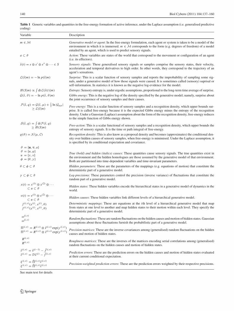
Table 1 Generic variables and quantities in the free-energy formation of active inference, under the Laplace assumption (i.e. generalised predictivecoding)

Variable Description

m ∈ M Generative model or agent: In the free-energy formulation, each agent or system is taken to be a model of theenvironment in which it is immersed. m ∈ M corresponds to the form (e.g. degrees of freedom) of a modelentailed by an agent, which is used to predict sensory signals.

a ⊂ ϑ Action: These variables are states of the world that correspond to the movement or configuration of an agent(i.e. its effectors).

s(t) = s ⊕ s′ ⊕ s′′ ⊕ · · · ∈ S Sensory signals: These generalised sensory signals or samples comprise the sensory states, their velocity,acceleration and temporal derivatives to high order. In other words, they correspond to the trajectory of anagent’s sensations.

L(s|m) = − ln p(s|m) Surprise: This is a scalar function of sensory samples and reports the improbability of sampling some sig-nals, under a generative model of how those signals were caused. It is sometimes called (sensory) suprisal orself-information. In statistics it is known as the negative log-evidence for the model.

H(S|m) ∝ ∫dtL(s(t)|m) Entropy: Sensory entropy is, under ergodic assumptions, proportional to the long-term time average of surprise.

G(s, ϑ) = − ln p(s, ϑ |m) Gibbs energy: This is the negative log of the density specified by the generative model; namely, surprise aboutthe joint occurrence of sensory samples and their causes.

F(s, q) = G(s, μ) + 12 ln |Gμμ|

≥ L(s|m)Free-energy: This is a scalar function of sensory samples and a recognition density, which upper bounds sur-prise. It is called free-energy because it is the expected Gibbs energy minus the entropy of the recognitiondensity. Under a Gaussian (Laplace) assumption about the form of the recognition density, free-energy reducesto the simple function of Gibbs energy shown.

S(s, q) = ∫dtF(s, q)

≥ H(S|m)Free-action: This is a scalar functional of sensory samples and a recognition density, which upper bounds theentropy of sensory signals. It is the time or path integral of free-energy.

q(ϑ) = N (μ, C) Recognition density: This is also know as a proposal density and becomes (approximates) the conditional den-sity over hidden causes of sensory samples, when free-energy is minimised. Under the Laplace assumption, itis specified by its conditional expectation and covariance.

ϑ = {u,ϕ, a}ϑ = {u, ϕ}u = {x, v}φ = {θ, γ }

True (bold) and hidden (italics) causes: These quantities cause sensory signals. The true quantities exist inthe environment and the hidden homologues are those assumed by the generative model of that environment.Both are partitioned into time-dependent variables and time-invariant parameters.

θ ⊂ φ ⊂ ϑ Hidden parameters: These are the parameters of the mappings (e.g. equations of motion) that constitute thedeterministic part of a generative model.

γ ⊂ φ ⊂ ϑ Log-precisions: These parameters control the precision (inverse variance) of fluctuations that constitute therandom part of a generative model.

x(t) = x (1) ⊕ x (2) ⊕ · · ·⊂ u ⊂ ϑ

Hidden states: These hidden variables encode the hierarchical states in a generative model of dynamics in theworld.

v(t) = v(1) ⊕ v(2) ⊕ · · ·⊂ u ⊂ ϑ

Hidden causes: These hidden variables link different levels of a hierarchical generative model.

f (i,v)(x (i), v(i), θ)

f (i,x)(x (i), v(i), θ)

Deterministic mappings: These are equations at the i th level of a hierarchical generative model that mapfrom states at one level to another and map hidden states to their motion within each level. They specify thedeterministic part of a generative model.

ω(i,v)

ω(i,x) Random fluctuations: These are random fluctuations on the hidden causes and motion of hidden states. Gaussianassumptions about these fluctuations furnish the probabilistic part of a generative model.

�(i,v) = R(i,v) ⊗ I (i,v) exp(γ (i,v))

�(i,x) = R(i,x) ⊗ I (i,x) exp(γ (i,x))Precision matrices: These are the inverse covariances among (generalised) random fluctuations on the hiddencauses and motion of hidden states.

R(i,v)

R(i,x) Roughness matrices: These are the inverses of the matrices encoding serial correlations among (generalised)random fluctuations on the hidden causes and motion of hidden states.

ε(i,v) = v(i−1) − f (i,v)

ε(i,x) = Dx (i) − f (i,x) Prediction errors: These are the prediction errors on the hidden causes and motion of hidden states evaluatedat their current conditional expectation.

ξ (i,v) = �(i,v)ε(i,v)

ξ (i,x) = �(i,x)ε(i,x) Precision-weighted prediction errors: These are the prediction errors weighted by their respective precisions.

See main text for details

123

Biol Cybern (2011) 104:137–160 141

entropy of their states and, implicitly, their sensory sam-ples of the world. More formally, any agent or model, m,

must minimise the average uncertainty (entropy) about itsgeneralised sensory states, s = s ⊕ s′ ⊕ s′′ ⊕ · · · ∈ S (⊕means concatenation). Generalised states (designated by thetilde) comprise the states per se and their generalised motion(velocity, acceleration, jerk, etc). Generalised motion is (inprinciple) of infinite order; however, it can be truncated to alow order (four in this paper); because the precision of highorder motion is very small. This is covered in detail in Friston(2008). The average uncertainty about generalised states is

H(S|m) = −∫

p(s|m) ln p(s|m)ds ∝∫

dtL(s(t)|m) (1)

Under ergodic assumptions, this is proportional to thelong-term average of surprise, also known as negativelog-evidence, L(s|m) = − ln p(s|m). Essentially, sensoryentropy accumulates negative log-evidence over time. Min-imising sensory entropy therefore corresponds to maximiz-ing the accumulated log-evidence for the agent’s model ofthe world. Although, sensory entropy cannot be minimiseddirectly, we can create an upper bound S(s, q) ≥ H(S|m)

that can be minimised. This bound is a function of a time-dependent recognition density q (ϑ) on the causes (i.e.environmental states and parameters) of sensory signals. Therequisite bound is the path-integral of free-energy F , whichis created simply by adding a non-negative function of therecognition density to surprise:

S =∫

dtF(s, q)

F = L + D(q(ϑ)||p(ϑ |s, m))

= 〈G〉q − HL = − ln p(s|m)

G = − ln p(s, ϑ |m)

H = −〈ln q(ϑ)〉q

(2)

This function is a Kullback–Leibler divergence D(·||·) andis greater than zero, with equality when q(ϑ) = p(ϑ |s, m)

is the true conditional density. This means that minimizingfree-energy, by changing the recognition density, makes itan approximate posterior or conditional density on sensorycauses. This is Bayes-optimal perception. The free-energycan be evaluated easily because it is a function of the recog-nition density and a generative model entailed by m: Eq. 2expresses free-energy in terms of H, the negentropy of q (ϑ)

and an energy G = − ln p(s, ϑ |m) expected under q(ϑ).This expected (Gibbs) energy rests on a probabilistic gen-erative model; p(s, ϑ |m). If we assume that the recognitiondensity q(ϑ) = N (μ, C) is Gaussian (known as the Laplaceassumption), we can express free-energy in terms of the con-ditional mean or expectation of the recognition density μ(t),where omitting constants

F(s(a), μ) = G(s, μ) + 1

2ln |Gμμ| (3)

Here, the conditional precision (inverse covariance) is C−1 =P = Gμμ. Crucially, this means the free-energy is a functionof the expected states and sensory samples, which depend onhow they are sampled by action. The action a(t) and expec-ted states μ(t) that minimise free-energy are the solutions tothe following differential equations

a = −Fa

˙μ = Dμ − Fμ

(4)

In short, the free-energy principle prescribes optimal actionand perception. Here D is a derivative matrix operator withidentity matrices above the leading diagonal, such that Dμ =μ′ ⊕ μ′′ ⊕ · · ·. Here and throughout, we assume all gradi-ents (denoted by subscripts) are evaluated at the mean. Thestationary solution of Eq. 4 ensures that when free-energy isminimised the expected motion of the states is the motionof the expected states; that is Fμ = 0 ⇒ ˙μ = Dμ. Therecognition dynamics in Eq. 4 can be regarded as a gradientdescent in a frame of reference that moves with the expectedmotion of the states (cf., surfing a wave). More general for-mulations of Eq. 4 make a distinction between time-varyingenvironmental states u ⊂ ϑ and time-invariant parametersϕ ⊂ ϑ (see Friston et al. 2010a,b). In this article, we willassume that only the states are unknown or hidden from theagent and ignore the learning of ϕ ⊂ ϑ

Action can only reduce free-energy by changing sensorysignals. This changes the first (log-likelihood) part of Gibb’senergy G = − ln p(s|ϑ, m)−ln p(ϑ |m) that depends on sen-sations. This means that action will sample sensory signalsthat are most likely under the recognition density (i.e. sam-pling selectively what one expects to experience). In otherwords, agents must necessarily (if implicitly) make infer-ences about the causes of their sensations and sample signalsthat are consistent with those inferences.

2.2 Summary

In summary, we have derived action and perception dynam-ics for expected states (in generalised coordinates of motion)that cause sensory samples. The solutions to these equa-tions minimise free-energy and therefore minimise surpris-ing sensations or, equivalently, maximise the evidence foran agent’s model of the world. This corresponds to activeinference, where predictions guide active sampling of sen-sory data. Active inference rests on the notion that “per-ception and behavior can interact synergistically, via theenvironment” to optimise behavior (Verschure et al. 2003)and is an example of self-referenced learning (Porr andWörgötter 2003; Wörgötter and Porr 2005). The precise formof active inference depends on the energy at each point in

123

142 Biol Cybern (2011) 104:137–160

time G = − ln p(s, ϑ |m) that rests on a particular generativemodel. In what follows, we review dynamic models of theworld.

2.3 Hierarchical dynamic models

We now introduce a general model based on the models dis-cussed in Friston (2008). We will assume that sensory dataare modeled with a special case of

s = f (v)(x, v, θ) + ω(v) : ω(v) ∼ N (0, �(v)(x, v, γ ))

x = f (x)(x, v, θ) + ω(x) : ω(x) ∼ N (0, �(x)(x, v, γ ))(5)

The nonlinear functions f (u) : u ∈ v, x represent the deter-ministic part of the model and are parameterised by θ ⊂ ϕ.The variables v ⊂ u are referred to as hidden causes, whilehidden states x ⊂ u meditate the influence of the causes onsensory data and endow the model with memory. Equation 5is just a state-space model, where the first (sensory map-ping) function maps from hidden variables to sensory dataand the second represents equations of motion for hiddenstates (where the hidden causes can be regarded as exoge-nous inputs). We assume the random fluctuations ω(u) areanalytic, such that the covariance of the generalised fluctu-ations ω(u) is well defined. These fluctuations represent thestochastic part of the model. This model allows for state-dependent changes in the amplitude of random fluctuationsand introduces a distinction between the effect of states onthe flow and dispersion of sensory trajectories. Under locallinearity assumptions, the generalised motion of the sensoryresponse and hidden states can be expressed compactly as

s = f (v) + z(v)

Dx = f (x) + z(x)(6)

where the generalised predictions are

f (u) =

⎡

⎢⎢⎢⎢⎣

f (u) = f (u)

f ′(u) = f (u)x x ′ + f (u)

v v′

f ′′(u) = f (u)x x ′′ + f (u)

v v′′...

⎤

⎥⎥⎥⎥⎦

(7)

Equation 5 means that Gaussian assumptions about the fluc-tuations specify a generative model in terms of a likelihoodand empirical priors on the motion of hidden states

p (s |x, v, ϕ, m ) = N(

f (v), �(v))

p (Dx |x, v, ϕ, m ) = N(

f (x), �(x)) (8)

These probability densities are encoded by their covari-ances �(u) or precisions (inverse covariances) �(u) :=�(x, v, γ (u)) with precision parameters γ ⊂ ϕ that controlthe amplitude and smoothness of the random fluctuations.Generally, the covariances factorise: �(u) = V (u) ⊗ �(u)

into a covariance among different fluctuations and a matrix ofcorrelations V (u) over different orders of motion that encodestheir smoothness. Given this generative model we can nowwrite down the energy as a function of the conditional means,which has a simple quadratic form (ignoring constants)

G = G(v) + G(x)

G(v) = 12 ε(v)T �(v)ε(v) − 1

2 ln |�(v)|G(x) = 1

2 ε(x)T �(x)ε(x) − 12 ln |�(x)| (9)

ε(v) = s − f (v)

ε(x) = Dμ(x) − f (x)

Here, the auxiliary variables ε(u) : u ∈ v, x are predictionerrors for sensory data and motion of the hidden states. Wenext consider hierarchical forms of this model. These are justspecial cases of Eq. 6, in which we make certain conditionalindependencies explicit. Although, the examples in the nextsection are not hierarchical, we briefly consider hierarchi-cal forms here, because they provide an important empiricalBayesian perspective on inference that may be exploited bythe brain. Furthermore, they provide a nice link to the con-nectionist scheme of Tani et al. (2004). Hierarchical dynamicmodels have the following form

s = f (1,v)(x (1), v(1), θ) + ω(1,v)

x (1) = f (1,x)(x (1), v(1), θ) + ω(1,x)

... (10)

v(i−1) = f (i,v)(x (i), v(i), θ) + ω(i,v)

x (i) = f (i,x)(x (i), v(i), θ) + ω(i,x)

As above, f (i,u) : u ∈ v, x are nonlinear functions, therandom terms ω(i,u) : u ∈ v, x are conditionally indepen-dent and enter each level of the hierarchy. They play therole of sensory noise at the first level and induce randomfluctuations in the states at higher levels. The hidden causesv = v(1) ⊕ v(2) ⊕ · · · link levels, whereas the hidden statesx = x (1) ⊕ x (2) ⊕ · · · link dynamics over time. In hierarchi-cal form, the output of one level acts as an input to the next.This input can enter nonlinearly to produce quite complicatedgeneralised convolutions with deep (hierarchical) structure.Crucially, when these top-down inputs act as control param-eters for the hidden states in the level below, they correspondto ‘parametric biases’ in the connectionist scheme of Taniet al. (2004). Hierarchical structure appears in the energy asempirical priors G(i,u) : u ∈ x, v where, ignoring constants

123

Biol Cybern (2011) 104:137–160 143

G =∑

i

G(i,v) +∑

i

G(i,x)

G(i,v) = 12 ε(i,v)T �(i,v)ε(i,v) − 1

2 ln |�(i,v)|G(i,x) = 1

2 ε(i,x)T �(i,x)ε(i,x) − 12 ln |�(i,x)| (11)

ε(i,v) = v(i−1) − f (i,v)

ε(i,x) = Dx (i) − f (i,x)

2.4 Summary

In summary, these models are as complicated as one couldimagine; they comprise hidden causes and states, whosedynamics can be coupled with arbitrary (analytic) nonlinearfunctions. Furthermore, these states can be subject to randomfluctuations with state-dependent changes in amplitude andarbitrary (analytic) autocorrelation functions. A key aspectis their hierarchical form, which induces empirical priors onthe causes. In the next section, we look at the recognitiondynamics entailed by this form of generative model, with aparticular focus on how recognition might be implementedin the brain.

2.5 Action and perception under hierarchical dynamicmodels

If we now write down the recognition dynamics (Eq. 4) usingprecision-weighted prediction errors ξ (i,u) = �(i,u)ε(i,u)

from Eq. 11, one can see the hierarchical message-passingentailed by this scheme (ignoring the derivatives of the energycurvature):

˙μ(i,v) = Dμ(i,v) + f i,vv

ξ (i,v) + f i,xv

ξ (i,x) − ξ (i+1,v)

˙μ(i,x) = Dμ(i,x) + f i,vx ξ (i,v) + f i,x

x ξ (i,x) − DT ξ (i,x)

ξ (i,v) = �(i,v)ε(i,v) = �(i,v)(μ(i−1,v) − f (i,v)

)

ξ (i,x) = �(i,x)ε(i,x) = �(i,x)(Dμ(i,x) − f (i,x)

)

(12)

For simplicity, we have assumed the amplitude of the ran-dom fluctuations does not depend on the states and canbe parameterised in terms of log-precisions γ (i,u) : u ∈v, x , where the precision of the generalised fluctuations is�(i,u) = R(i,u)⊗ I (i,u) exp(γ (i,u)). Here, R(i,u) is the inverseof the correlation matrix V (i,u) above and I (i,u) is the identitymatrix.

It is difficult to overstate the generality and importanceof Eq. 12: It grandfathers nearly every known statisticalscheme, under parametric assumptions about noise. Theserange from ordinary least squares to advanced variationaldeconvolution schemes (see Friston 2008). Equation 12is generalised predictive coding and follows simply fromthe generalised gradient decent in Eq. 4, where the free-energy gradients reduce to linear mixtures of prediction

errors. This simplicity rests on Gaussian assumptions aboutthe random fluctuations and the form of the recognitiondensity.

Equation 12 shows how recognition dynamics can beimplemented by relatively simple message-passing between(neuronal) states encoding conditional expectations and pre-diction errors. The motion of conditional expectations isdriven in a linear fashion by prediction error, while predictionerror is a nonlinear function of conditional expectations. Inneural network terms, Eq. 12 says that error-units encoding(precision-weighted) prediction error receive messages fromthe state-units encoding conditional expectations in the samelevel and the level above. Conversely, state-units are drivenby error-units in the same level and the level below. Crucially,perception requires only the (precision-weighted) predictionerror from the lower level ξ (i,v) and the level in questionξ (i,x), ξ (i+1,v). These constitute bottom-up and lateral mes-sages that drive the conditional expectations μ(i,u) towardsa better prediction. These top-down and lateral predictionscorrespond to f (i,u). This is the essence of recurrent message-passing between hierarchical levels to optimise free-energyor suppress prediction error (see Friston 2008 for a moredetailed discussion).

Equation 12 also tells us that the precisions modulate theresponses of the error-units to their presynaptic inputs. Thistranslates into synaptic gain control in principal cells (super-ficial pyramidal cells; Mumford 1992) elaborating predictionerrors and fits comfortably with modulatory bias effects thathave been associated with attention (Desimone and Duncan1995; Schroeder et al. 2001; Salinas and Sejnowski 2001;Fries et al. 2008; see Feldman and Friston 2010). We willuse precisions later to contextualise recognition under actionor observation.

Since action can only affect the free-energy by changingsensory data, it can only affect sensory prediction error. FromEq. 4, we have

a = −ε(v)a ξ (v)

ε(v)a = f (v)

x

∑

j

D− j ( f (x)

x ) j−1 f (x)a

(13)

The second equality expresses the change in prediction errorwith action in terms of the effect of action on successivelyhigher order motions of the hidden states. In biologicallyplausible instances of this scheme, the partial derivatives inEq. 13 would have to be computed on the basis of a map-ping from action to sensory consequences, which is usuallyquite simple, e.g. activating an intrafusal muscle fiber elic-its stretch receptor activity in the corresponding spindle (seeFriston et al. 2010a for discussion).

123

144 Biol Cybern (2011) 104:137–160

2.6 Summary

In summary, we have derived equations for the dynamicsof action and perception using a free-energy formulation ofadaptive (Bayes-optimal) exchange with the world and a gen-erative model that is both generic and biologically plausible.In what follows, we will use Eqs. 12 and 13 to simulate neu-ronal responses under action and observation. A technicaltreatment of the material in section will be found in Fristonet al. (2010b), which provides the details of the scheme usedto integrate (solve) Eq. 12 to produce the simulations in thenext section.

3 Simulations: action

In this section, we describe a generative model of handwrit-ing and then use the generalised predictive coding schemeof the previous section to simulate neuronal dynamics andbehavior. To create these simulations, all we have to do isspecify the equations of the generative model and the preci-sion of random fluctuations. Action and perception are thenprescribed by Eqs. 12 and 13, which simulate neuronal andbehavioral responses respectively. Our agent was equipped asimple (one-level) dynamical model of its sensorium basedon a Lotka–Volterra model of itinerant dynamics. The partic-ular form of this model has been discussed previously as thebasis of putative speech decoding (Kiebel et al. 2009b). Here,it is used to model a stable heteroclinic channel (Rabinovichet al. 2008) encoding successive locations to which the agentexpects its two-jointed arm to be attracted. The resulting tra-jectory was contrived to simulate synthetic handwriting.

A stable heteroclinic channel is a particular form of (sta-ble) itinerant trajectory or orbit that revisits a sequence of(unstable) fixed points. In our model, there are two sets ofhidden states. The first set α = [α1, . . . , α6]T ⊂ x corre-sponds to the state-space of a Lotka–Volterra system. Thisis an abstract (attractor) state-space, in which a series ofattracting points are visited in succession. The second set{x1, x2, x ′

1, x ′2} ⊂ x corresponds to the (angular) positions

and velocities of the two joints in (two dimensional) phys-ical space. The dynamics of both sets are coupled throughthe agent’s prior expectation that the arm will be drawn toa particular location, ∗(α) specified by the attractor states.This is implemented simply by placing a (virtual) elastic bandbetween the tip of the arm and the attracting location in physi-cal space. The hidden states basically draw the arm’s extrem-ity (finger) to a succession of locations to produce an orbit ortrajectory, under classical Newtonian mechanics. We chosethe locations so that the resulting trajectory looked like hand-writing. These hidden states generate both proprioceptiveand visual (extroceptive) sensory data: The proprioceptivedata are the angular positions and velocities of the two joints

{x1, x2, x ′1, x ′

2}, while the visual information was the locationof the arm in Cartesian space { 1, 1+ 2}, where 2(x1, x2) isthe displacement of the finger from the location of the secondjoint 1(x1) (see Fig. 1 and Table 2). Crucially, because thisgenerative model generates two (proprioceptive and visual)sensory modalities, solutions to the equations of the previoussection (i.e. perception) implement Bayes-optimal multisen-sory integration. However, because action is also trying toreduce prediction errors, it will move the arm to reproducethe expected trajectory (under the constraints of the motorplant). In other words, the arm will trace out a trajectoryprescribed by the itinerant priors. This closes the loop, pro-ducing autonomous self-generated sequences of behavior ofthe sort described below. Note that the real world does notcontain any attracting locations or elastic bands: The onlycauses of observed movement are the self-fulfilling expec-tations encoded by the itinerant dynamics of the generativemodel. In short, hidden attractor states essentially entail theintended movement trajectory, because they generate predic-tions that action fulfils. This means expected states encodeconditional percepts (concepts) about latent abstract states(that do not exist in the absence of action), which play therole of intentions. We now describe the model formally. Inthis model, there is only one hierarchical level, and we candrop the hierarchical superscripts.

3.1 The generative model

The model used in this section concerns a two-joint arm.When simulating active inference, it is important to distin-guish between the agent’s generative model and the actualdynamics generating sensory data. To make this distinctionclear, we will use bold for true equations and states, whilethose of the generative model will be written in italics. Propri-oceptive input corresponds to the angular position and veloc-ity of both joints, while the visual input corresponds to thelocation of the extremities of both parts of the arm.

f (v) = f (v) =

⎡

⎢⎢⎢⎢⎢⎢⎣

x1

x2

x ′1

x ′2

1(x)

1(x) + 2(x)

⎤

⎥⎥⎥⎥⎥⎥⎦

(14)

We ignore the complexities of inference on retinotopicallymapped visual input and assume the agent has direct accessto locations of the arm in visual space. The kinetics of thearm conforms to Newtonian laws, under which action forcesthe angular position of each joint. Both joints have an equi-librium position at 90◦; with inertia ml ∈ 8, 4 and viscosityκi ∈ 4, 2, giving the following equations of motion

123

Biol Cybern (2011) 104:137–160 145

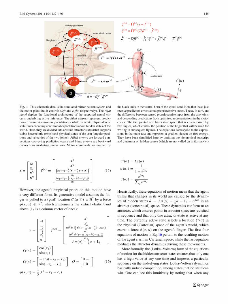
Fig. 1 This schematic details the simulated mirror neuron system andthe motor plant that it controls (left and right, respectively). The rightpanel depicts the functional architecture of the supposed neural cir-cuits underlying active inference. The filled ellipses represent predic-tion error-units (neurons or populations), while the white ellipses denotestate-units encoding conditional expectations about hidden states of theworld. Here, they are divided into abstract attractor states (that supportsstable heteroclinic orbits) and physical states of the arm (angular posi-tions and velocities of the two joints). Filled arrows are forward con-nections conveying prediction errors and black arrows are backwardconnections mediating predictions. Motor commands are emitted by

the black units in the ventral horn of the spinal cord. Note that these justreceive prediction errors about proprioceptive states. These, in turn, arethe difference between sensed proprioceptive input from the two jointsand descending predictions from optimised representations in the motorcortex. The two jointed arm has a state space that is characterised bytwo angles, which control the position of the finger that will be used forwriting in subsequent figures. The equations correspond to the expres-sions in the main text and represent a gradient decent on free-energy.They have been simplified here by omitting the hierarchical subscriptand dynamics on hidden causes (which are not called on in this model)

x =

⎡

⎢⎢⎣

x1

x2

x′1x′2

⎤

⎥⎥⎦ f (x) =

⎡

⎢⎢⎢⎢⎣

x′1x′2

(a1+v1− 1

4 (x1− π2 )−κ1x′

1

)

m1(a2+v2− 1

4 (x2− π2 )−κ2x′

2)

m2

⎤

⎥⎥⎥⎥⎦

(15)

However, the agent’s empirical priors on this motion havea very different form. Its generative model assumes the fin-ger is pulled to a (goal) location ∗(α(t)) ∈ �2 by a forceφ(x, α) ∈ �2, which implements the virtual elastic bandabove (16 is a column vector of ones):

x =

⎡

⎢⎢⎢⎢⎣

x1

x2

x ′1

x ′2

α

⎤

⎥⎥⎥⎥⎦

f (x) =

⎡

⎢⎢⎢⎢⎢⎢⎣

x ′1

x ′2

(φT 2 T2 O 1− 1

16 (x1− π2 )−κ1x ′

1)

m1(φT O 2− 1

16 (x2− π2 )−κ2x ′

2)

m2

Aσ(α) − 18α + 16

⎤

⎥⎥⎥⎥⎥⎥⎦

1(x) =[

cos(x1)

sin(x1)

]

2(x) =[− cos(−x2 − x1)

sin(−x2 − x1)

]

O =[

0 −11 0

]

(16)

φ(x, α) = 1

2( ∗ − 1 − 2)

∗(α) = Ls(α)

σ (αi ) = 1

1 + e2αi

s(αi ) = e2αi

∑j e2α j

Heuristically, these equations of motion mean that the agentthinks that changes in its world are caused by the dynam-ics of hidden states α = Aσ(α) − 1

8α + 16 + ω(α) in anabstract (conceptual) space. These dynamics conform to anattractor, which ensures points in attractor space are revisitedin sequence and that only one attractor-state is active at anytime. The currently active state selects a location ∗(α) inthe physical (Cartesian) space of the agent’s world, whichexerts a force φ(x, α) on the agent’s finger. The first fourequations of motion in Eq. 16 pertain to the resulting motionof the agent’s arm in Cartesian space, while the last equationmediates the attractor dynamics driving these movements.

More formally, the (Lotka–Volterra) form of the equationsof motion for the hidden attractor states ensures that only onehas a high value at any one time and imposes a particularsequence on the underlying states. Lotka–Volterra dynamicsbasically induce competition among states that no state canwin. One can see this intuitively by noting that when any

123

146 Biol Cybern (2011) 104:137–160

Table 2 Variables and quantities specific to the writing example ofactive inference (see main text for details)

Variable Description

α(t) ∈ �6 ⊂ x Hidden attractor states: A vector of hiddenstates that specify the current locationtowards which the agent expects its arm tobe pulled.

xi (t) ∈ � ⊂ xx ′

i (t) ∈ � ⊂ x Hidden effector states: Hidden states thatspecify the angular position and velocity ofthe i-th joint in a two-jointed arm.

1(x1) ∈ �2

2(x1, x2) ∈ �2 Joint locations: Locations of the end of thetwo arm parts in Cartesian space. These arefunctions of the angular positions of thejoints.

∗(α(t)) ∈ �2 Attracting location: The location towardswhich the arm is drawn. This is specified bythe hidden attractor states.

φ(x, α) ∈ �2 Newtonian force: This is the angular force onthe joints exerted by the attracting location.

A ∈ �6×6 ⊂ θ Attractor parameters: A matrix of parametersthat govern the (sequential Lotka–Volterra)dynamics of the hidden attractor states.

L ∈ �2×6 ⊂ θ Cartesian parameters: A matrix ofparameters that specify the attractinglocations associated with each hiddenattractor state.

state’s value is high, the negative effect on its motion cannow longer be offset by the upper bounded function σ(α).The resulting winnerless competition rests on the (logistic)function σ(α), while the sequence order is determined by theelements of the matrix

A =

⎡

⎢⎢⎢⎢⎢⎢⎣

0 − 12 −1 −1 · · ·

− 32 0 − 1

2 −1

−1 − 32 0 − 1

2. . .

−1 −1 − 32 0

.... . .

. . .

⎤

⎥⎥⎥⎥⎥⎥⎦

(17)

Each attractor state has an associated location in Cartesianspace, which draws the arm towards it using classical New-tonian mechanics. The attracting location is specified by amapping ∗(α) = Ls(α) from attractor space α ∈ �6 toCartesian space ∈ �2, which weights the locations L ⊂ θ :

L =[

1 1.1 1.0 1 1.4 0.91 1.2 0.4 1 0.9 1.0

]

(18)

with a softmax function s(α) of the attractor states. The loca-tion parameters were specified by hand but could, in princi-ple, be learnt as described in Friston et al. (2009, 2010a).The inertia and viscosity of the arm were chosen some-what arbitrarily to reproduce realistic writing movementsover 256 time bins, each corresponding to roughly 8 ms (i.e. asecond). Unless stated otherwise, we used a log-precision of

four for sensory noise and eight for fluctuations in the motionof hidden states.

Movement is caused by action, which is trying to min-imise sensory prediction error. A subtle but important con-straint in these simulations was that action only had access toproprioceptive prediction error. In other words, action onlyminimised the difference between the expected and sensedangular location and velocity of the joints. This is importantbecause it resolves a potential problem with active inference;namely that action or command signals need to know howthey affect sensory input to minimise prediction error. Theargument here is that the mapping from action to its proprio-ceptive consequences is sufficiently simple that it can be rel-egated (by evolution) to peripheral motor systems (perhapseven the spinal cord). In this example, complicated (hand-writing) behavior is prescribed just by proprioceptive (gen-eralised joint position) prediction errors. Here the mappingbetween action (changing the generalised joint position) andproprioceptive input is very simple. However, this does notmean that visual information (prediction errors) cannot affectaction. Visual information is crucial when optimizing condi-tional beliefs (expected states) that prescribe predictions inboth proprioceptive and visual modalities. This means thatvisual input can influence action vicariously, through highlevel (intentional) representations that predict a (unimodal)proprioceptive component (Fig. 1). See also Todorov et al.(2005). In short, although the perception or intention of theagent integrates proprioceptive and visual information in aBayes-optimal fashion, action is driven just by proprioceptiveprediction errors. This will become important in the next sec-tion, where we remove proprioceptive input but retain visualstimulation to simulate action observation.

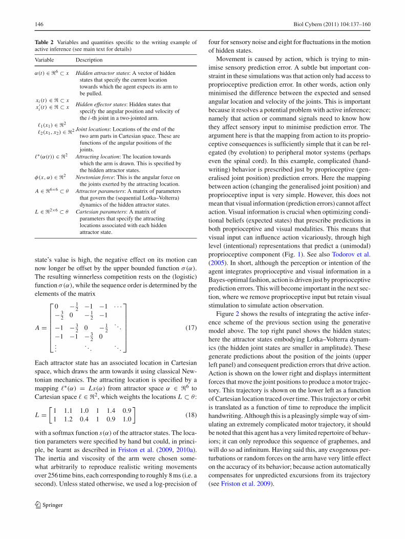
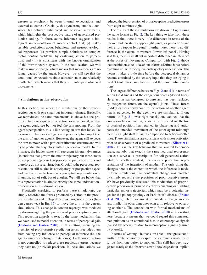
Figure 2 shows the results of integrating the active infer-ence scheme of the previous section using the generativemodel above. The top right panel shows the hidden states;here the attractor states embodying Lotka–Volterra dynam-ics (the hidden joint states are smaller in amplitude). Thesegenerate predictions about the position of the joints (upperleft panel) and consequent prediction errors that drive action.Action is shown on the lower right and displays intermittentforces that move the joint positions to produce a motor trajec-tory. This trajectory is shown on the lower left as a functionof Cartesian location traced over time. This trajectory or orbitis translated as a function of time to reproduce the implicithandwriting. Although this is a pleasingly simple way of sim-ulating an extremely complicated motor trajectory, it shouldbe noted that this agent has a very limited repertoire of behav-iors; it can only reproduce this sequence of graphemes, andwill do so ad infinitum. Having said this, any exogenous per-turbations or random forces on the arm have very little effecton the accuracy of its behavior; because action automaticallycompensates for unpredicted excursions from its trajectory(see Friston et al. 2009).

123

Biol Cybern (2011) 104:137–160 147

50 100 150 200 250-0.5

0

0.5

1

1.5

2prediction and error

time

50 100 150 200 250-8

-6

-4

-2

0

2

4hidden states

time

-0.5 0 0.5 1 1.5

0

0.5

1

1.5

2

movement

location

50 100 150 200 250-0.4

-0.3

-0.2

-0.1

0

0.1

0.2

0.3

time

perturbation and action

loca

tion

( )a t

A B

C D

Fig. 2 This figure shows the results of simulated action (writing),under active inference, in terms of conditional expectations about hid-den states of the world (b), consequent predictions about sensory input(a) and the ensuing behavior (c) that is caused by action (d). The autono-mous dynamics that underlie this behavior rest upon the expected hiddenstates that follow Lotka–Volterra dynamics: these are the six (arbitrarily)colored lines in b. The hidden physical states have smaller amplitudesand map directly on to the predicted proprioceptive and visual signals(a). The visual locations of the two joints are shown as blue and greenlines, above the predicted joint positions and angular velocities thatfluctuate around zero. The dotted lines correspond to prediction error,

which shows small fluctuations about the prediction. Action tries tosuppress this error by ‘matching’ expected changes in angular velocitythrough exerting forces on the joints. These forces are shown in blueand green in d. The dotted line corresponds to exogenous forces, whichwere omitted in this example. The subsequent movement of the arm istraced out in c; this trajectory has been plotted in a moving frame ofreference so that it looks like synthetic handwriting (e.g. a successionof ‘j’ and ‘a’ letters). The straight lines in c denote the final position ofthe two jointed arm and the hand icon shows the final position of itsextremity. (Color figure online)

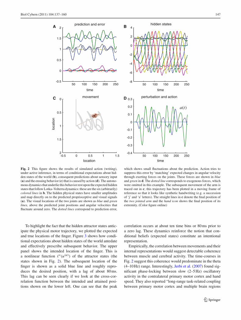
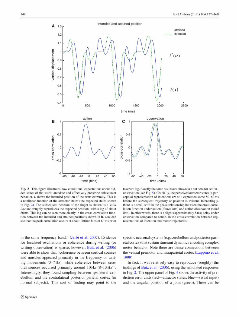
To highlight the fact that the hidden attractor states antic-ipate the physical motor trajectory, we plotted the expectedand true locations of the finger. Figure 3 shows how condi-tional expectations about hidden states of the world antedateand effectively prescribe subsequent behavior. The upperpanel shows the intended location of the finger. This isa nonlinear function ∗(u(α)) of the attractor states (thestates shown in Fig. 2). The subsequent location of thefinger is shown as a solid blue line and roughly repro-duces the desired position, with a lag of about 80 ms.This lag can be seen clearly if we look at the cross-cor-relation function between the intended and attained posi-tions shown on the lower left. One can see that the peak

correlation occurs at about ten time bins or 80 ms prior toa zero lag. These dynamics reinforce the notion that con-ditional beliefs (expected states) constitute an intentionalrepresentation.

Empirically, the correlation between movements and theirinternal representations would suggest detectable coherencebetween muscle and cerebral activity. The time-courses inFig. 2 suggest this coherence would predominate in the theta(4–10 Hz) range. Interestingly, Jerbi et al. (2007) found sig-nificant phase-locking between slow (2–5 Hz) oscillatoryactivity in the contralateral primary motor cortex and handspeed. They also reported “long-range task-related couplingbetween primary motor cortex and multiple brain regions

123

148 Biol Cybern (2011) 104:137–160

-60 -40 -20 0 20 40 60-1

-0.5

0

0.5

1action

time (bins)

cros

s-co

rrel

atio

n

-60 -40 -20 0 20 40 60-1

-0.5

0

0.5

1observation

time (bins)

cros

s-co

rrel

atio

n

0 500 1000 1500 2000 25000.4

0.5

0.6

0.7

0.8

0.9

1

1.1

1.2

1.3

time (ms)

vert

ical

dis

plac

emen

t

intended and attained position

attainedintended

A

B C

Fig. 3 This figure illustrates how conditional expectations about hid-den states of the world antedate and effectively prescribe subsequentbehavior. a shows the intended position of the arms extremity. This isa nonlinear function of the attractor states (the expected states shownin Fig. 2). The subsequent position of the finger is shown as a solidline and roughly reproduces the expected position, with a lag of about80 ms. This lag can be seen more clearly in the cross-correlation func-tion between the intended and attained positions shown in b. One cansee that the peak correlation occurs at about 10 time bins or 80 ms prior

to a zero lag. Exactly the same results are shown in c but here for action–observation (see Fig. 5). Crucially, the perceived attractor states (a per-ceptual representation of intention) are still expressed some 50–60 msbefore the subsequent trajectory or position is evident. Interestingly,there is a small shift in the phase relationship between the cross-corre-lation function under action (dotted line) and action observation (solidline). In other words, there is a slight (approximately 8 ms) delay underobservation compared to action, in the cross-correlation between rep-resentations of intention and motor trajectories

in the same frequency band.” (Jerbi et al. 2007). Evidencefor localised oscillations or coherence during writing (orwriting observation) is sparse; however, Butz et al. (2006)were able to show that “coherence between cortical sourcesand muscles appeared primarily in the frequency of writ-ing movements (3–7 Hz), while coherence between cere-bral sources occurred primarily around 10 Hz (8–13 Hz)”.Interestingly, they found coupling between ipsilateral cer-ebellum and the contralateral posterior parietal cortex (innormal subjects). This sort of finding may point to the

specific neuronal systems (e.g. cerebellum and posterior pari-etal cortex) that sustain itinerant dynamics encoding complexmotor behavior. Note there are dense connections betweenthe ventral premotor and intraparietal cortex (Luppino et al.1999).

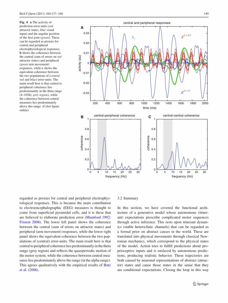
In fact, it was relatively easy to reproduce (roughly) thefindings of Butz et al. (2006), using the simulated responsesin Fig. 2. The upper panel of Fig. 4 shows the activity of pre-diction error units (red—attractor states; blue—visual input)and the angular position of a joint (green). These can be

123

Biol Cybern (2011) 104:137–160 149

Fig. 4 a The activity ofprediction error units (redattractor states, blue visualinput) and the angular positionof the first joint (green). Thesecan be regarded as proxies forcentral and peripheralelectrophysiological responses;b shows the coherence betweenthe central (sum of errors on redattractor states) and peripheral(green arm movement)responses, while c shows theequivalent coherence betweenthe two populations of (centralred and blue) error-units. Themain result here is that central toperipheral coherence liespredominantly in the theta range(4–10 Hz; grey region), whilethe coherence between centralmeasures lies predominatelyabove this range. (Color figureonline)

200 400 600 800 1000 1200 1400 1600 1800 2000

-0.03

-0.02

-0.01

0

0.01

0.02

0.03

central and peripheral responses

time (ms)

activ

ity (

au)

0 5 10 15 20 25 300

0.2

0.4

0.6

0.8

1central-peripheral coherence

frequency (Hz)

cohe

renc

e

0 5 10 15 20 25 300

0.2

0.4

0.6

0.8

1central-central coherence

frequency (Hz)

cohe

renc

e

x αε

vε

ix

A

B C

regarded as proxies for central and peripheral electrophys-iological responses. This is because the main contributionto electroencephalographic (EEG) measures is thought tocome from superficial pyramidal cells, and it is these thatare believed to elaborate prediction error (Mumford 1992;Friston 2008). The lower left panel shows the coherencebetween the central (sum of errors on attractor states) andperipheral (arm movement) responses, while the lower rightpanel shows the equivalent coherence between the two pop-ulations of (central) error-units. The main result here is thatcentral to peripheral coherence lies predominantly in the thetarange (grey region) and reflects the quasiperiodic motion ofthe motor system, while the coherence between central mea-sures lies predominately above the range (in the alpha range).This agrees qualitatively with the empirical results of Butzet al. (2006).

3.2 Summary

In this section, we have covered the functional archi-tecture of a generative model whose autonomous (itiner-ant) expectations prescribe complicated motor sequencesthrough active inference. This rests upon itinerant dynam-ics (stable heteroclinic channels) that can be regarded asa formal prior on abstract causes in the world. These aretranslated into physical movements through classical New-tonian mechanics, which correspond to the physical statesof the model. Action tries to fulfill predictions about pro-prioceptive inputs and is enslaved by autonomous predic-tions, producing realistic behavior. These trajectories areboth caused by neuronal representations of abstract (attrac-tor) states and cause those states in the sense that theyare conditional expectations. Closing the loop in this way

123

150 Biol Cybern (2011) 104:137–160

ensures a synchrony between internal expectations andexternal outcomes. Crucially, this synchrony entails a con-sistent lag between anticipated and observed movements,which highlights the prospective nature of generalised pre-dictive coding. In short, active inference suggests a bio-logical implementation of motor control that; (i) makestestable predictions about behavioral and neurophysiologi-cal responses; (ii) provides simple solutions to complexmotor control problems, by enslaving action to percep-tion; and (iii) is consistent with the known organizationof the mirror-neuron system. In the next section, we willmake a simple change which means that movements are nolonger caused by the agent. However, we will see that theconditional expectations about attractor states are relativelyunaffected, which means that they still anticipate observedmovements.

4 Simulations: action–observation

In this section, we repeat the simulations of the previoussection but with one small but important change. Basically,we reproduced the same movements as above but the pro-prioceptive consequences of action were removed, so thatthe agent could see but not feel the arm moving. From theagent’s perspective, this is like seeing an arm that looks likeits own arm but does not generate proprioceptive input (i.e.the arm of another agent). However, the agent still expectsthe arm to move with a particular itinerant structure and willtry to predict the trajectory with its generative model. In thisinstance, the hidden states still represent itinerant dynamics(intentions) that govern the motor trajectory but these statesdo not produce (precise) proprioceptive prediction errors andtherefore do not result in action. Crucially, the perceptual rep-resentation still retains its anticipatory or prospective aspectand can therefore be taken as a perceptual representation ofintention, not of self, but of another. We will see below thatthis representation is almost exactly the same under action–observation as it is during action.

Practically speaking, to perform these simulations, wesimply recorded the forces produced by action in the previ-ous simulation and replayed them as exogenous forces (hid-den causes v(t) in Eq. 15) to move the arm in the currentsimulations. This change in context (agency) was modeledby down-weighting the precision of proprioceptive signals.This reduction appeals to exactly the same mechanism thatwe have used to model attention, in terms of perceptual gain(Feldman and Friston 2010). In this setting, reducing theprecision of proprioceptive prediction errors precludes themfrom having any influence on perceptual inference (i.e. theagent cannot feel changes in its joints). Furthermore, actionis not compelled to reduce these prediction errors becausethey have no (or trivial) precision. In these simulations, we

reduced the log-precision of proprioceptive prediction errorsfrom eight to minus eight.

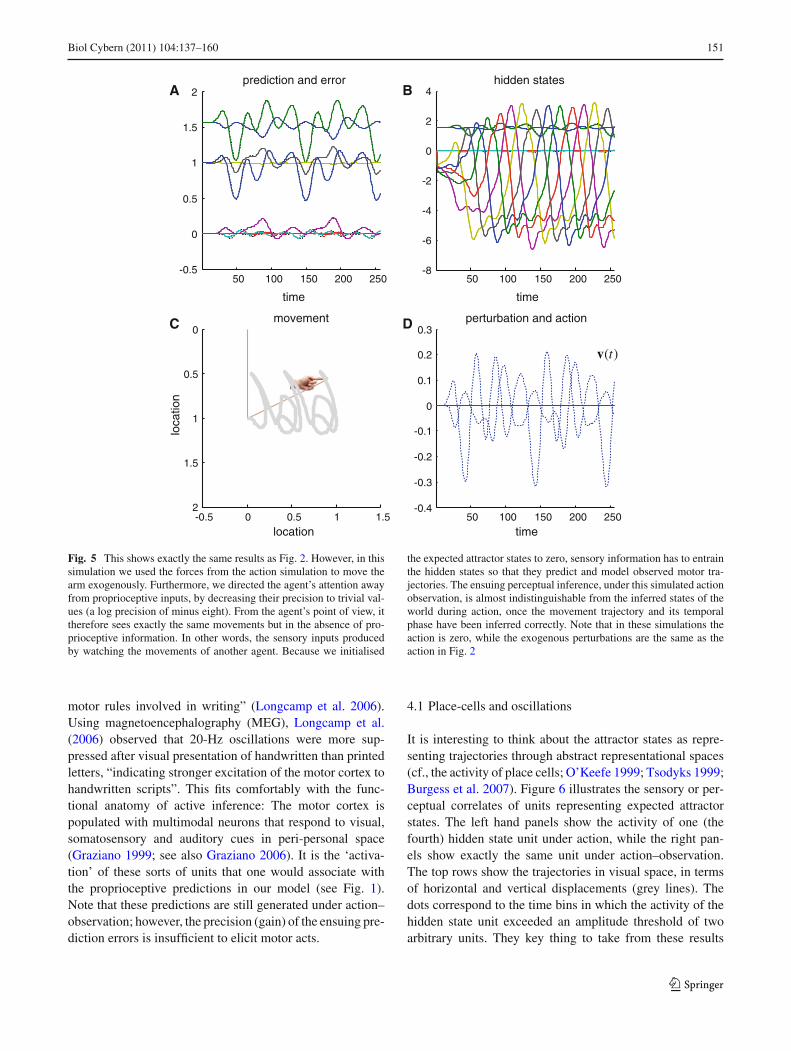
The results of these simulations are shown in Fig. 5 usingthe same format as Fig. 2. The key thing to take from theseresults is that there is very little difference in terms of theinferred hidden states (upper right panel) or predictions andtheir errors (upper left panel). Furthermore, there is no dif-ference in the actual movement (lower left panel). Havingsaid this, there is small but important difference in inferenceat the onset of movement: Comparison with Fig. 2 showsthat the hidden states take about 400 ms (50 time bins) before‘catching up’ with the equivalent trajectory under action. Thismeans it takes a little time before the perceptual dynamicsbecome entrained by the sensory input that they are trying topredict (note these simulations used the same initial condi-tions)

The largest difference between Figs. 2 and 5 is in terms ofaction (sold lines) and the exogenous forces (dotted lines).Here, action has collapsed to zero and has been replacedby exogenous forces on the agent’s joints. These forces(hidden causes) correspond to the action of another agentthat is perceived by the agent we are simulating. If onereturns to Fig. 3 (lower right panel), one can see that thecross-correlation function, between the expected and the trueor attained position, has retained its phase-lag and antici-pates the intended movement of the other agent (althoughthere is a slight shift in lag in comparison to action—dottedline). These simulations are consistent with motor activationprior to observation of a predicted movement (Kilner et al.2004). This is the key behavior that we wanted to demon-strate; namely, that exactly the same neuronal representa-tion can serve as a prescription for self-generated action,while, in another context, it encodes a perceptual repre-sentation of the intentions of another. The only thing thatchanges here is the context in which the inference is made.In these simulations, this contextual change was modeledby simply reducing the precision of proprioceptive errors.We have previously discussed this modulation of proprio-ceptive precision in terms of selectively enabling or disablingparticular motor trajectories, which may be a potential tar-get for the pathophysiology of Parkinson’s disease (Fristonet al. 2009). Here, we use it to encode a change in con-text implicit in observing ones own arm, relative to observ-ing another’s. The connection with formal mechanisms ofattentional gain (Feldman and Friston 2010) is interestinghere, because it means that we could regard this contextualmanipulation as an attentional bias to exteroceptive signals(caused by others) relative to interoceptive signals (causedby oneself).

In terms of writing, “humans are able to recognise hand-written texts accurately despite the extreme variability ofscripts from one writer to another. This skill has been sug-gested to rely on the observer’s own knowledge about implicit

123

Biol Cybern (2011) 104:137–160 151

50 100 150 200 250-0.5

0

0.5

1

1.5

2prediction and error

time

50 100 150 200 250-8

-6

-4

-2

0

2

4hidden states

time

-0.5 0 0.5 1 1.5

0

0.5

1

1.5

2

movement

location50 100 150 200 250

-0.4

-0.3

-0.2

-0.1

0

0.1

0.2

0.3

time

perturbation and action

loca

tion

( )tv

A B

C D

Fig. 5 This shows exactly the same results as Fig. 2. However, in thissimulation we used the forces from the action simulation to move thearm exogenously. Furthermore, we directed the agent’s attention awayfrom proprioceptive inputs, by decreasing their precision to trivial val-ues (a log precision of minus eight). From the agent’s point of view, ittherefore sees exactly the same movements but in the absence of pro-prioceptive information. In other words, the sensory inputs producedby watching the movements of another agent. Because we initialised

the expected attractor states to zero, sensory information has to entrainthe hidden states so that they predict and model observed motor tra-jectories. The ensuing perceptual inference, under this simulated actionobservation, is almost indistinguishable from the inferred states of theworld during action, once the movement trajectory and its temporalphase have been inferred correctly. Note that in these simulations theaction is zero, while the exogenous perturbations are the same as theaction in Fig. 2

motor rules involved in writing” (Longcamp et al. 2006).Using magnetoencephalography (MEG), Longcamp et al.(2006) observed that 20-Hz oscillations were more sup-pressed after visual presentation of handwritten than printedletters, “indicating stronger excitation of the motor cortex tohandwritten scripts”. This fits comfortably with the func-tional anatomy of active inference: The motor cortex ispopulated with multimodal neurons that respond to visual,somatosensory and auditory cues in peri-personal space(Graziano 1999; see also Graziano 2006). It is the ‘activa-tion’ of these sorts of units that one would associate withthe proprioceptive predictions in our model (see Fig. 1).Note that these predictions are still generated under action–observation; however, the precision (gain) of the ensuing pre-diction errors is insufficient to elicit motor acts.

4.1 Place-cells and oscillations

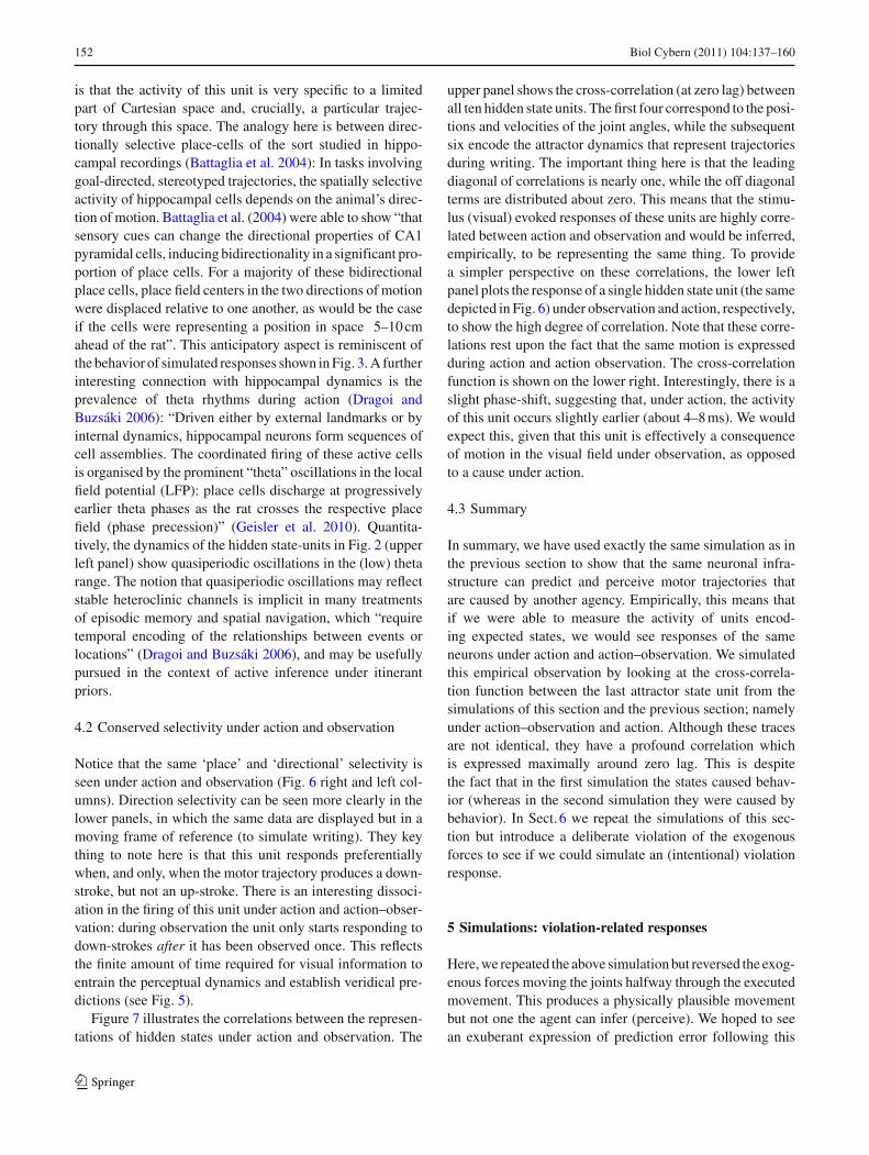
It is interesting to think about the attractor states as repre-senting trajectories through abstract representational spaces(cf., the activity of place cells; O’Keefe 1999; Tsodyks 1999;Burgess et al. 2007). Figure 6 illustrates the sensory or per-ceptual correlates of units representing expected attractorstates. The left hand panels show the activity of one (thefourth) hidden state unit under action, while the right pan-els show exactly the same unit under action–observation.The top rows show the trajectories in visual space, in termsof horizontal and vertical displacements (grey lines). Thedots correspond to the time bins in which the activity of thehidden state unit exceeded an amplitude threshold of twoarbitrary units. They key thing to take from these results

123

152 Biol Cybern (2011) 104:137–160

is that the activity of this unit is very specific to a limitedpart of Cartesian space and, crucially, a particular trajec-tory through this space. The analogy here is between direc-tionally selective place-cells of the sort studied in hippo-campal recordings (Battaglia et al. 2004): In tasks involvinggoal-directed, stereotyped trajectories, the spatially selectiveactivity of hippocampal cells depends on the animal’s direc-tion of motion. Battaglia et al. (2004) were able to show “thatsensory cues can change the directional properties of CA1pyramidal cells, inducing bidirectionality in a significant pro-portion of place cells. For a majority of these bidirectionalplace cells, place field centers in the two directions of motionwere displaced relative to one another, as would be the caseif the cells were representing a position in space 5–10 cmahead of the rat”. This anticipatory aspect is reminiscent ofthe behavior of simulated responses shown in Fig. 3. A furtherinteresting connection with hippocampal dynamics is theprevalence of theta rhythms during action (Dragoi andBuzsáki 2006): “Driven either by external landmarks or byinternal dynamics, hippocampal neurons form sequences ofcell assemblies. The coordinated firing of these active cellsis organised by the prominent “theta” oscillations in the localfield potential (LFP): place cells discharge at progressivelyearlier theta phases as the rat crosses the respective placefield (phase precession)” (Geisler et al. 2010). Quantita-tively, the dynamics of the hidden state-units in Fig. 2 (upperleft panel) show quasiperiodic oscillations in the (low) thetarange. The notion that quasiperiodic oscillations may reflectstable heteroclinic channels is implicit in many treatmentsof episodic memory and spatial navigation, which “requiretemporal encoding of the relationships between events orlocations” (Dragoi and Buzsáki 2006), and may be usefullypursued in the context of active inference under itinerantpriors.

4.2 Conserved selectivity under action and observation

Notice that the same ‘place’ and ‘directional’ selectivity isseen under action and observation (Fig. 6 right and left col-umns). Direction selectivity can be seen more clearly in thelower panels, in which the same data are displayed but in amoving frame of reference (to simulate writing). They keything to note here is that this unit responds preferentiallywhen, and only, when the motor trajectory produces a down-stroke, but not an up-stroke. There is an interesting dissoci-ation in the firing of this unit under action and action–obser-vation: during observation the unit only starts responding todown-strokes after it has been observed once. This reflectsthe finite amount of time required for visual information toentrain the perceptual dynamics and establish veridical pre-dictions (see Fig. 5).

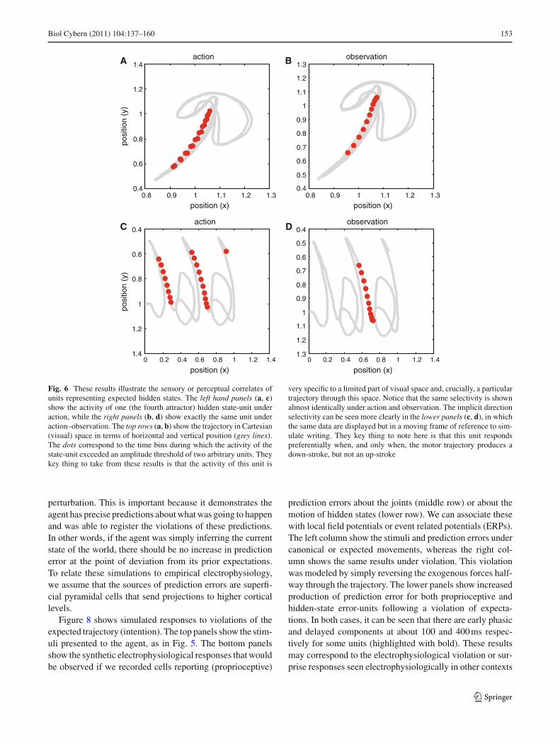
Figure 7 illustrates the correlations between the represen-tations of hidden states under action and observation. The

upper panel shows the cross-correlation (at zero lag) betweenall ten hidden state units. The first four correspond to the posi-tions and velocities of the joint angles, while the subsequentsix encode the attractor dynamics that represent trajectoriesduring writing. The important thing here is that the leadingdiagonal of correlations is nearly one, while the off diagonalterms are distributed about zero. This means that the stimu-lus (visual) evoked responses of these units are highly corre-lated between action and observation and would be inferred,empirically, to be representing the same thing. To providea simpler perspective on these correlations, the lower leftpanel plots the response of a single hidden state unit (the samedepicted in Fig. 6) under observation and action, respectively,to show the high degree of correlation. Note that these corre-lations rest upon the fact that the same motion is expressedduring action and action observation. The cross-correlationfunction is shown on the lower right. Interestingly, there is aslight phase-shift, suggesting that, under action, the activityof this unit occurs slightly earlier (about 4–8 ms). We wouldexpect this, given that this unit is effectively a consequenceof motion in the visual field under observation, as opposedto a cause under action.

4.3 Summary

In summary, we have used exactly the same simulation as inthe previous section to show that the same neuronal infra-structure can predict and perceive motor trajectories thatare caused by another agency. Empirically, this means thatif we were able to measure the activity of units encod-ing expected states, we would see responses of the sameneurons under action and action–observation. We simulatedthis empirical observation by looking at the cross-correla-tion function between the last attractor state unit from thesimulations of this section and the previous section; namelyunder action–observation and action. Although these tracesare not identical, they have a profound correlation whichis expressed maximally around zero lag. This is despitethe fact that in the first simulation the states caused behav-ior (whereas in the second simulation they were caused bybehavior). In Sect. 6 we repeat the simulations of this sec-tion but introduce a deliberate violation of the exogenousforces to see if we could simulate an (intentional) violationresponse.

5 Simulations: violation-related responses

Here, we repeated the above simulation but reversed the exog-enous forces moving the joints halfway through the executedmovement. This produces a physically plausible movementbut not one the agent can infer (perceive). We hoped to seean exuberant expression of prediction error following this

123

Biol Cybern (2011) 104:137–160 153

0.8 0.9 1 1.1 1.2 1.30.4

0.6

0.8

1

1.2

1.4action

position (x)

posi

tion

(y)

0.8 0.9 1 1.1 1.2 1.30.4

0.5

0.6

0.7

0.8

0.9

1

1.1

1.2

1.3observation

position (x)

0 0.2 0.4 0.6 0.8 1 1.2 1.4

0.4

0.6

0.8

1

1.2

1.4

action

position (x)

posi

tion

(y)

0 0.2 0.4 0.6 0.8 1 1.2 1.4

0.4

0.5

0.6

0.7

0.8

0.9

1

1.1

1.2

1.3

observation

position (x)

A B

C D

Fig. 6 These results illustrate the sensory or perceptual correlates ofunits representing expected hidden states. The left hand panels (a, c)show the activity of one (the fourth attractor) hidden state-unit underaction, while the right panels (b, d) show exactly the same unit underaction–observation. The top rows (a, b) show the trajectory in Cartesian(visual) space in terms of horizontal and vertical position (grey lines).The dots correspond to the time bins during which the activity of thestate-unit exceeded an amplitude threshold of two arbitrary units. Theykey thing to take from these results is that the activity of this unit is

very specific to a limited part of visual space and, crucially, a particulartrajectory through this space. Notice that the same selectivity is shownalmost identically under action and observation. The implicit directionselectivity can be seen more clearly in the lower panels (c, d), in whichthe same data are displayed but in a moving frame of reference to sim-ulate writing. They key thing to note here is that this unit respondspreferentially when, and only when, the motor trajectory produces adown-stroke, but not an up-stroke

perturbation. This is important because it demonstrates theagent has precise predictions about what was going to happenand was able to register the violations of these predictions.In other words, if the agent was simply inferring the currentstate of the world, there should be no increase in predictionerror at the point of deviation from its prior expectations.To relate these simulations to empirical electrophysiology,we assume that the sources of prediction errors are superfi-cial pyramidal cells that send projections to higher corticallevels.

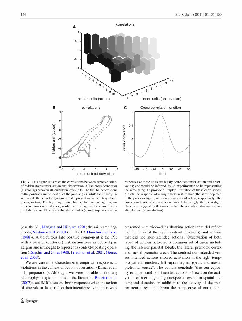
Figure 8 shows simulated responses to violations of theexpected trajectory (intention). The top panels show the stim-uli presented to the agent, as in Fig. 5. The bottom panelsshow the synthetic electrophysiological responses that wouldbe observed if we recorded cells reporting (proprioceptive)

prediction errors about the joints (middle row) or about themotion of hidden states (lower row). We can associate thesewith local field potentials or event related potentials (ERPs).The left column show the stimuli and prediction errors undercanonical or expected movements, whereas the right col-umn shows the same results under violation. This violationwas modeled by simply reversing the exogenous forces half-way through the trajectory. The lower panels show increasedproduction of prediction error for both proprioceptive andhidden-state error-units following a violation of expecta-tions. In both cases, it can be seen that there are early phasicand delayed components at about 100 and 400 ms respec-tively for some units (highlighted with bold). These resultsmay correspond to the electrophysiological violation or sur-prise responses seen electrophysiologically in other contexts

123

154 Biol Cybern (2011) 104:137–160

1 23

4 56

7 89

10

12

34

56

78

910

-1

-0.5

0

0.5

1

hidden units (observation)

correlations

hidden units (action)

-6 -4 -2 0 2 4-8

-6

-4

-2

0

2

4correlations

hidden unit (observation)

hidd

en u

nit (

actio

n)

-60 -40 -20 0 20 40 60-1

-0.5

0

0.5

1Cross-correlation function

time

cros

s-co

rrel

atio

n

A

B C

Fig. 7 This figure illustrates the correlations between representationsof hidden states under action and observation. a The cross-correlation(at zero lag) between all ten hidden state-units. The first four correspondto the positions and velocities of the joint angles, while the subsequentsix encode the attractor dynamics that represent movement trajectoriesduring writing. The key thing to note here is that the leading diagonalof correlations is nearly one, while the off-diagonal terms are distrib-uted about zero. This means that the stimulus (visual) input-dependent

responses of these units are highly correlated under action and obser-vation; and would be inferred, by an experimenter, to be representingthe same thing. To provide a simpler illustration of these correlations,b plots the response of a single hidden state unit (the same depictedin the previous figure) under observation and action, respectively. Thecross-correlation function is shown in c. Interestingly, there is a slightphase shift suggesting that under action the activity of this unit occursslightly later (about 4–8 ms)

(e.g. the N1, Mangun and Hillyard 1991; the mismatch neg-ativity, Näätänen et al. (2001) and the P3, Donchin and Coles(1988)). A ubiquitous late positive component it the P3bwith a parietal (posterior) distribution seen in oddball par-adigms and is thought to represent a context-updating opera-tion (Donchin and Coles 1988; Friedman et al. 2001; Gómezet al. 2008).

We are currently characterizing empirical responses toviolations in the context of action–observation (Kilner et al.,– in preparation). Although, we were not able to find anyelectrophysiological studies in the literature, Buccino et al.(2007) used fMRI to assess brain responses when the actionsof others do or do not reflect their intentions: “volunteers were

presented with video-clips showing actions that did reflectthe intention of the agent (intended actions) and actionsthat did not (non-intended actions). Observation of bothtypes of actions activated a common set of areas includ-ing the inferior parietal lobule, the lateral premotor cortexand mesial premotor areas. The contrast non-intended ver-sus intended actions showed activation in the right temp-oro-parietal junction, left supramarginal gyrus, and mesialprefrontal cortex”. The authors conclude “that our capac-ity to understand non intended actions is based on the acti-vation of areas signaling unexpected events in spatial andtemporal domains, in addition to the activity of the mir-ror neuron system”. From the perspective of our model,

123

Biol Cybern (2011) 104:137–160 155

-0.5 0 0.5 1 1.5

0

0.5

1

1.5

2

observation

-0.5 0 0.5 1 1.5

0

0.5

1

1.5

2

violation

-400 -200 0 200 400 600-0.04

-0.02

0

0.02

0.04

0.06proprioceptive error

-400 -200 0 200 400 600-0.04

-0.02

0

0.02

0.04

0.06proprioceptive error

pred

ictio

n er

ror

-400 -200 0 200 400 600-0.015

-0.01

-0.005

0

0.005

0.01

0.015

0.02error on hidden states

time (ms)

pred

ictio

n er

ror

-400 -200 0 200 400 600-0.015

-0.01

-0.005

0

0.005

0.01

0.015

0.02error on hidden states

time (ms)

vε

xε

A

C

E F

D

B

Fig. 8 This figure shows simulated electrophysiological responses toviolations of expected movements. The top panels (a, b) show the stim-uli presented to the agent as in Fig. 5. The lower panels show the syn-thetic electrophysiological responses of units reporting prediction error(c, d proprioceptive errors; e, f errors on the motion of hidden states).The left panels (a, c, e) show the stimuli and prediction errors undercanonical or expected movements, whereas the right panels (b, d, f)show the same results with a violation. This violation was modeled by

simply reversing the exogenous forces halfway through the writing. Theexuberant production of prediction error is shown in d and e. It can beseen here that there is an early phasic and delayed components at about100 and 400 ms for at least one proprioceptive and hidden state error-unit (sold lines). In c and d, errors on the angular positions are show inblue and green, while errors on angular velocities are in red and cyan.All errors on hidden states are shown in red in e and f. (Color figureonline)

the greater expression of prediction error under violation(i.e. non-intended action) would suggest fMRI activation (asopposed to deactivation) in those areas reporting predictionerrors on biological motion and proprioception. These wouldprobably involve the parietal and temporal cortex (as reportedin Buccino et al. 2007).

5.1 Summary

In this section, we simulated violation responses in terms ofsynthetic ERPs. These responses speak to an empirical han-dle on action–observation responses, particularly in relationto how they rest upon encoding the intentions (anticipated

123

156 Biol Cybern (2011) 104:137–160

trajectory) of motor movements. Crucially, these responsesshould be observed in exactly the same neuronal populationsresponsible for generating predictions that drive the samebehavior during action. Although a simple set of simulations,they address a potentially important empirical approach to thestudy of mirror-neuron system.

6 Discussion

In this article, we have tried to show that the mirror-neuronsystem is entirely consistent and understandable in the con-text of (Bayes-optimal) active inference under the free-energy principle. Put simply, under this formulation, the braindoes not represent intended motor acts or the perceptual con-sequences of those acts separately; the constructs representedin the brain are both intentional and perceptual: They areamodal inferences about the states of the world generatingsensory data that have both sensory and motor correlates,depending upon the context in which they are made. Thepredictions generated by these representations are modal-ity-specific, prescribing both exteroceptive (e.g. visual) andinteroceptive (e.g. proprioception) predictions, which actionfulfils. The functional segregation of motor and sensory cor-tex could be regarded as a hierarchical decomposition, in thebrain’s model of its world, which provides predictions thatare primarily sensory (e.g. visual cortex) or proprioceptive(motor and premotor cortex). If true, this means that highlevel representations can be used to furnish predictions ineither visual or proprioceptive modalities, depending uponthe context in which those predictions are called upon.

The ideas in this article can be regarded as a generic Bayes-ian (free-energy) perspective on the connectionist schemeintroduced by Tani (2003); see also Tani et al. (2004) andWeber et al. (2006). Using robotic experiments, Tani et al.(2004) show that multiple behavioral schemata can be learnedby recurrent neural networks in a distributed and hierarchicalmanner. Hierarchical (parametric) biases in the network playan essential role in both generating and recognizing behav-ioral patterns. “They act as a mirror system by means of self-organizing adequate memory structures”. We have pursuedthe same basic idea; that hierarchical generative models ofthe (interoceptive and exteroceptive) sequelae of action canbe used to generate and recognise action and exploit this ideato understand what mirror neurons may encode.

The simulations in this article suggest that in the contextof self-agency, proprioceptive predictions are afforded a highbias or precision, whereas when observing another this biasis suppressed (gated). Exactly the same sort of bias hasbeen proposed for action selection by fronto-striatal loops(e.g. Bogacz and Gurney 2007; Frank et al. 2007; Hazyet al. 2007). Interestingly these proposals call upon classicalneuromodulators (like dopamine and noradrenalin), whose

role in modulating synaptic efficacy is exactly what wouldbe required to implement expected precision in generalisedpredictive coding (see Eq. 12 and Friston 2008). Formallyrelated mechanisms proposed for attention (e.g. Reynoldsand Heeger 2009; Friston 2008; Feldman and Friston 2010)may also depend on modulatory neurotransmission (Clarket al. 1989; Coull 1998; Dalley et al. 2001; Davidson andMarrocco 2000; Hasselmo and Giocomo 2006; Herrero et al.2008) and indeed the basal forebrain (Voytko et al. 1994).This means that we can use the same generative model, underaction or observation, by selectively attending to visual orproprioceptive information (depending upon whether visualmovement is caused by ourselves or others). The only differ-ence, from the point of view of inference, is that movementscaused by others do not have proprioceptive components.This provides a simple but mechanistic account of mirrorneuron responses in the context of Bayes-optimal inference.Note that the gating of the proprioceptive prediction errorsdoes not imply that the primary and secondary somatosen-sory areas are quiescent during action observation. Rather,that any observed activity in these areas should be suppressedrelative to higher somatosensory processing. This is preciselywhat has been observed. In a meta-analysis of activations inprimary and secondary somatosensory cortices during obser-vation of touching actions: Keysers et al. (2010) report thatareas OP1 and OP4 that constitute the secondary somatosen-sory area are consistently found to be active when observingactions. Areas BA1 and BA2—of the primary somatosensorycortex are sometimes found to be active—whereas area BA3of the primary somatosensory cortex has never been shownto be active during observation of an action. Area BA3 isthe primary area for somatosensory input where as BA1 andBA2 receive their inputs from BA3.

6.1 Active inference and motor control

There have been several accounts of forward and inversemodels in action–observation in the motor control litera-ture (Wolpert et al. 2003; Flanagan et al. 2003; Miall 2003;Keysers and Perrett 2004): “Skilled motor behavior relies onthe brain learning both to control the body and predict theconsequences of this control. Prediction turns motor com-mands into expected sensory consequences, whereas controlturns desired consequences into motor commands. To cap-ture this symmetry, the neural processes underlying predic-tion and control are termed the forward and inverse internalmodels, respectively” (Flanagan et al. 2003). Forward andinverse models (e.g. Wolpert et al. 1995) have been discussedin relation to imitation: The logic here is that the inversemodel (mapping from sensory consequences to motor com-mands) can be used as a recognition model to infer the causeof an observed action. Once the cause is inferred the actioncan then be imitated. Although these proposals for forward-

123

Biol Cybern (2011) 104:137–160 157

inverse models in imitation and social interactions (Wolpertet al. 2003) are exciting; they are formally very different fromactive inference and related connectionist schemes (Tani et al.2004; Friston et al. 2010a). In active inference (and predictivecoding), there are no inverse models or controllers; a gen-erative model mapping from intention (cause) to sensation(consequence) is inverted by suppressing prediction error. Ifthis suppression calls on action, then the intention is the gen-erated action. If not, the intention (of another) is recognised.The implicit inversion depends on self-organizing, reciprocalexchange of signals among hierarchical levels of the brain’sgenerative model (see Fig. 1 and Tani et al. 2004). Crucially,active inference does not invoke any ‘desired consequences’,its rests only on experience-dependent learning and infer-ence: Experience induces prior expectations, which guideperceptual inference and action:

Although our focus has been on the implications of activeinference for the mirror-neuron system and vice versa, theapproach taken in this work also has implications for conven-tional theories of motor control. In conventional approaches,one usually starts with some desired states or end points ofthe control process and uses an inverse model to computethe optimal control signals. These control signals are some-times finessed with corrections based upon a forward model(mapping from the control signals to expected sensory sig-nals). This is a more complicated architecture than that usedin active inference, where predictions control movement andobviate the need for an explicit control signal. This simpli-fies things greatly and resolves a series of issues in the motorcontrol literature, which we have not emphasised in this arti-cle. For example, the problem of how to control a motor plantwith many degrees of freedom becomes rather trivial. Here, itwas solved by an invisible elastic band connecting the fingerto the desired location. The ensuing scheme is a formal exten-sion of the equilibrium point hypothesis that suggests “actionand perception are accomplished in a common spatial frameof reference” (Feldman 2009). We generalise equilibriumpoints to cover trajectories through the use of generalisedmotion (generalised predictive coding). From the perspec-tive of inferring the motor intentions of others, generalisedpredictive coding has an interesting implication. It suggeststhat an agent will only be able to predict (in the generalised oranticipatory sense) the trajectories or intentions of another,if the observed agent has the same sort of motor apparatus.In short, one should be much better at inferring the intendedbehavior of con-specifics, because the exteroceptive predic-tions are based on a veridical model of the other’s motorplant. This is not to say that we cannot predict the behaviorof other creatures; however, it is unlikely that the neuronsinvolved will show mirror neuron like properties, becausethey cannot predict our own proprioceptive inputs. This mayprovide an interesting empirical prediction; in that one wouldexpect fewer violation responses when observing the same

biological motion subtended by agents that do and do notlook like ourselves (cf., Miura et al. 2010).

6.2 Functional anatomy

In describing these simulations, we have portrayed itinerant(attractor) dynamics as encoding motor intentions (antici-pated or expected motor trajectories), while considering theirrole during action–observation as consequent on their role inspecifying behavior. However, from a neurodevelopmentalperspective the converse may be true. In other words, theform and structure of these neural attractor networks may beoptimised during experience-dependent learning by watch-ing other con-specifics (cf., Lee et al. 2010; see also DelGiudice et al. 2009). By subsequently attending to proprio-ceptive inputs one can see how learning to act through imita-tion could exploit the amodal role of high-order (intentional)representations. Clearly, this rests upon representations thatpredict the visual consequences of movement (of others):Neurons in the superior temporal sulcus (STS), respondselectively to biological movement (Grossman et al. 2000),both in monkeys (Oram and Perrett 1994) and humans (Alli-son et al. 2000). These neurons are not mirror neuronsbecause they do not discharge during action execution. Nev-ertheless, they are often considered part of the mirror-neuronsystem (Keysers and Perrett 2004). Although mirror neuronswere first discovered in macaque monkeys, using single-cellrecordings, there is evidence for a homologous system inhumans: Functional magnetic resonance imaging and posi-tron emission tomography studies demonstrate that areas offrontal cortex, inferior parietal lobule (and posterior parietalcortex) and STS are active during action–observation (e.g.Decety et al. 1997; Grèzes et al. 2001; Hamilton and Grafton2006).

We have deliberately tried to keep our simulations as sim-ple as possible to highlight the underlying ideas. There aremany things that one could nuance to make these simulationsmore realistic; for example, using a hierarchy of stable het-eroclinic channels (cf., Tani et al. 2004; Kiebel et al. 2009b)and providing explicit contextual cues about whether onewas observing ones own body or another’s. However, thebasic results would not change and, even under this simplemodel, there is an easy mapping to known neurobiology. Forexample, we could associate the dynamics encoding itinerantmotor sequences with prefrontal neurons (e.g. F5 in mon-keys or Broca’s area in man). Many people have noted thatthe same form of itinerant trajectories used to predict com-plex motor sequences may also be involved in the predictionof speech (see Arbib 2010; Borghi et al. 2010). The hid-den states subtending biological motion may correspond toneuronal populations in V5 complex and superior temporalsulcus (Allison et al. 2000; Takahashi et al. 2008), whilelow level proprioceptive and visual predictions could be

123

158 Biol Cybern (2011) 104:137–160

associated with the activity of units in the motor cortex andearly visual system respectively. The distributed anatomicalarrangement of these representations speaks to a mirror-neu-ron system that implicates both executive systems and corti-cal systems involved in the processing of biological motion,which we have previously discussed in relation to mirror-neuron responses and inference about the intention of others(Kilner et al. 2007a,b). In conclusion, we hope to have sub-stantiated previous conjectures about the mirror-neuron sys-tem in the context of Bayesian inference, using simulationsto disclose some operational and mechanistic details.

Acknowledgements This work was funded by the Wellcome Trust.We would like to thank Marcia Bennett for helping prepare this manu-script and our colleagues for very useful discussions, particularly StefanKiebel and Jun Tani. We would also like to thank our two reviewers forhelpful guidance

7 Appendix (software note)

This article has focused on the heuristics and basic equa-tions that underlie active inference. However, we anticipatethat people may want to reproduce and extend the simu-lations presented in this paper. In principle, this is fairlystraightforward because active inference just entails integrat-ing (solving) Eq. 4. The particular form of Eq. 4 rests on thefree-energy gradients, which are specified completely by thegenerative model (specified as the equations of motion andGaussian priors on the parameters of those equations). Thenumerics underlying the integration of Eq. 4 are described inFriston et al. 2010a (Eq. A3.2) and the form of the gradientscan be found in Feldman and Friston (2010): See Appendix1: Integrating the recognition dynamics (generalised filter-ing); using exactly the same notion as in this article. A moretechnical account can be found in Friston et al. (2010b) thatdescribes recognition dynamics in terms of generalised fil-tering. Active inference can be regarded as supplementinggeneralised filtering (recognition dynamics) with the actiondynamics in Eq. 13.

For people who want to reproduce the simulations and seehow they work at a technical level, we recommend that theystart with the Matlab code used in this article: All the requi-site routines are available as part of the SPM software (aca-demic freeware released under a GNU license; http://www.fil.ion.ucl.ac.uk/spm). In particular, the graphics in this papercan be reproduced from a graphical user interface (GUI) inthe DEM toolbox that is invoked by typing DEM_demoat the Matlab prompt. When the GUI appears, depress theaction observation button. The GUI provides the option torun or view/edit routines that serve as a pseudo-code specifi-cation of the ideas in the main text. DEM stands for dynamicexpectation maximization, which is a variant of generalisedfiltering that uses a mean-field approximation (see Friston

et al. 2010b for details). The GUI and the scripts are anno-tated in a way that should help clarify how the simulationsare assembled.

It may seem strange to bundle simulation routines witha data analysis package; however, there are several rea-sons for doing this. (i) Active inference (as implement inspm_ADEM.m) uses exactly the same architecture and sub-routines as the equivalent DEM and generalised filteringschemes that omit action (spm_DEM.m and spm_LAP.m,respectively). These schemes are used routinely to analyzeempirical time-series as part of the analysis software. Thishighlights the fact that active inference appeals to exactlythe same fundaments of evidence-based model optimization(and variational techniques) as state-of-the-art Bayesian fil-tering for empirical data. (ii) Because the neurobiologicalsimulation and data analysis routines call on the same num-erics and sub-functions it is easier to bundle them together.This has the advantage that improvements to the code (anddebugging) are seen by both application domains. One ofthe reasons we encourage people to start with this code isthat it has been tested extensively through worldwide dis-semination in the neuroimaging community. (iii) We haveestablished a protocol within SPM, where people can createlinks to their own SPM compatible toolboxes, which is a niceway to disseminate ideas and developments. This may proveuseful for people interested in the computational aspects ofactive inference in the future. (iv) Finally, the simulations arethemselves used as part of data analysis; where recognitiondynamics are used to explain evoked electromagnetic brainsignals (see spm_dcm_dem.m).

References

Afraimovich V, Tristan I, Huerta R, Rabinovich MI (2008) Winnerlesscompetition principle and prediction of the transient dynamics ina Lotka–Volterra model. Chaos 18(4):043103

Allison T, Puce A, McCarthy G (2000) Social perception from visualcues: role of the STS region. Trends Cogn Sci 4:267–278

Arbib MA (2008) From grasp to language: embodied concepts and thechallenge of abstraction. J Physiol (Paris) 102(1–3):4–20

Arbib MA (2010) Mirror system activity for action and language isembedded in the integration of dorsal and ventral pathways. BrainLang 112(1):12–24

Ballard DH, Hinton GE, Sejnowski TJ (1983) Parallel visual computa-tion. Nature 306:21–26

Battaglia FP, Sutherland GR, McNaughton BL (2004) Local sensorycues and place cell directionality: additional evidence of prospec-tive coding in the hippocampus. J Neurosci 24(19):4541–4550

Bogacz R, Gurney K (2007) The basal ganglia and cortex implementoptimal decision making between alternative actions. Neural Com-put 19(2):442–477

Borghi AM, Gianelli C, Scorolli C (2010) Sentence comprehension:effectors and goals, self and others. An overview of experimentsand implications for robotics. Front Neurorobot 4:3 Jun 14

123

Biol Cybern (2011) 104:137–160 159

Buccino G, Baumgaertner A, Colle L, Büchel C, Rizzolatti G, BinkofskiF (2007) The neural basis for understanding non-intended actions.Neuroimage. 36(Suppl 2):T119–T127

Burgess N, Barry C, O’Keefe J (2007) An oscillatory interferencemodel of grid cell firing. Hippocampus 17(9):801–812

Butz M, Timmermann L, Gross J, Pollok B, Dirks M, Hefter H,Schnitzler A (2006) Oscillatory coupling in writing and writer’scramp. J Physiol Paris 99(1):14–20

Clark CR, Geffen GM, Geffen LB (1989) Catecholamines and thecovert orientation of attention in humans. Neuropsychologia27:131–139

Coull JT (1998) Neural correlates of attention and arousal: insightsfrom electrophysiology, functional neuroimaging and psychophar-macology. Prog Neurobiol 55:343–361

Dalley JW, McGaughy J, O’Connell MT, Cardinal RN, Levita L,Robbins TW (2001) Distinct changes in cortical acetylcholine andnoradrenaline efflux during contingent and noncontingent perfor-mance of a visual attentional task. J Neurosci 21:4908–4914

Davidson MC, Marrocco RT (2000) Local infusion of scopolamine intointraparietal cortex slows covert orienting in rhesus monkeys. JNeurophysiol 83:1536–1549

Dayan P, Hinton GE, Neal RM (1995) The Helmholtz machine. NeuralComput 7:889–904

Decety J, Grèzes J, Costes N, Perani D, Jeannerod M, Procyk E, Grassi F,Fazio F (1997) Brain activity during observation of actions. Influ-ence of action content and subject’s strategy. Brain 120:1763–1777

Del Giudice M, Manera V, Keysers C (2009) Programmed to learn?The ontogeny of mirror neurons. Dev Sci 12(2):350–363

Desimone R, Duncan J (1995) Neural mechanisms of selective visualattention. Annu Rev Neurosci 18:193–222

Di Pellegrino G, Fadiga L, Fogassi L, Gallese V, Rizzolatti G(1992) Understanding motor events: a neurophysiological study.Exp Brain Res 91:176–180

Donchin E, Coles MGH (1988) Is the P300 component a manifestationof context updating?. Behav Brain Sci 11:355–372

Dragoi G, Buzsáki G (2006) Temporal encoding of place sequences byhippocampal cell assemblies. Neuron 50(1):145–157

Feldman AG (2009) New insights into action-perception coupling. ExpBrain Res 194(1):39–58

Feldman H, Friston K (2010) Attention, uncertainty and free-energy.Front Hum Neurosci 4:215. doi:10.3389/fnhum.2010.00215

Flanagan JR, Vetter P, Johansson RS, Wolpert DM (2003) Predictionprecedes control in motor learning. Curr Biol 13(2):146–150

Fogassi L, Ferrari PF, Gesierich B, Rozzi S, Chersi F, Rizzolatti G(2005) Parietal lobe: from action organization to intention under-standing. Science 308:662–667

Frank MJ, Scheres A, Sherman SJ (2007) Understanding decision-mak-ing deficits in neurological conditions: insights from models ofnatural action selection. Philos Trans R Soc Lond B Biol Sci362(1485):1641–1654

Friedman D, Cycowicz YM, Gaeta H (2001) The novelty P3: an event-related brain potential (ERP) sign of the brain’s evaluation of nov-elty. Neurosci Biobehav Rev 25:355–373

Fries P, Womelsdorf T, Oostenveld R, Desimone R (2008) The effectsof visual stimulation and selective visual attention on rhyth-mic neuronal synchronization in macaque area V4. J Neurosci28(18):4823–4835

Friston K (2008) Hierarchical models in the brain. PLoS Comput Biol4(11):e1000211

Friston K (2009) The free-energy principle: a rough guide to the brain?.Trends Cogn Sci 13(7):293–301

Friston K, Kilner J, Harrison L (2006) A free energy principle for thebrain. J Physiol (Paris) 100(1–3):70–87

Friston KJ, Daunizeau J, Kiebel SJ (2009) Reinforcement learning oractive inference?. PLoS One 4(7):e6421

Friston KJ, Daunizeau J, Kilner J, Kiebel SJ (2010a) Action and behav-ior: a free-energy formulation. Biol Cybern 102(3):227–260

Friston K, Stephan K, Li B, Daunizeau J (2010b) Generalised filtering.Math Prob Eng. Article ID 621670

Frith CD, Frith U (1999) Interacting minds—a biological basis. Science286:1692–1695

Gallese V, Goldman A (1998) Mirror-neurons and the simulation the-ory of mind reading. Trends Cogn Sci 2:493–501

Gallese V, Fadiga L, Fogassi L, G Rizzolatti (1996) Action recognitionin the premotor cortex. Brain 119:593–609

Geisler C, Diba K, Pastalkova E, Mizuseki K, Royer S, BuzsákiG (2010) Temporal delays among place cells determine the fre-quency of population theta oscillations in the hippocampus. ProcNatl Acad Sci USA 107(17):7957–7962

Gómez CM, Flores A, Digiacomo MR, Ledesma A, González-RosaJ (2008) P3a and P3b components associated to the neurocognitiveevaluation of invalidly cued targets. Neurosci Lett 430:181–185

Grafton ST, Hamilton AF (2007) Evidence for a distributed hierar-chy of action representation in the brain. Hum Mov Sci 26(4):590–616

Graziano MS (1999) Where is my arm? The relative role of vision andproprioception in the neuronal representation of limb position.Proc Natl Acad Sci USA 96(18):10418–10421

Graziano M (2006) The organization of behavioral repertoire in motorcortex. Annu Rev Neurosci 29:105–134

Gregory RL (1968) Perceptual illusions and brain models. Proc R SocLond B 171:179–196

Gregory RL (1980) Perceptions as hypotheses. Phil Trans R Soc LondB 290:181–197

Grèzes J, Fonlupt P, Bertenthal B, Delon-Martin C, Segebarth C,Decety J (2001) Does perception of biological motion rely on spe-cific brain regions?. Neuroimage 13:775–785

Grossman E, Donnelly M, Price R, Pickens D, Morgan V, Neighbor G,Blake R (2000) Brain areas involved in perception of biologicalmotion. J Cogn Neurosci 12:711–720

Hamilton AF, Grafton ST (2006) Goal representation in human anteriorintraparietal sulcus. J Neurosci 26:1133–1137

Hasselmo ME, Giocomo LM (2006) Cholinergic modulation of corticalfunction. J Mol Neurosci 30(1–2):133–135

Hazy TE, Frank MJ, O’reilly RC (2007) Towards an executive with-out a homunculus: computational models of the prefrontal cor-tex/basal ganglia system. Philos Trans R Soc Lond B Biol Sci362(1485):1601–1613

Herrero JL, Roberts MJ, Delicato LS, Gieselmann MA, Dayan P, ThieleA (2008) Acetylcholine contributes through muscarinic receptorsto attentional modulation in V1. Nature 454:1110–1114

Ijspeert JA, Nakanishi J, Schaal S (2002) Movement imitation withnonlinear dynamical systems in humanoid robots. In InternationalConference on Robotics and Automation (ICRA 2002), pp 1398–1403

Jeannerod M, Arbib MA, Rizzolatti G, Sakata H (1995) Graspingobjects: the cortical mechanisms of visuomotor transformation.Trends Neurosci 18(7):314–320

Jerbi K, Lachaux JP, N’Diaye K, Pantazis D, Leahy RM, GarneroL, Baillet S (2007) Coherent neural representation of hand speedin humans revealed by MEG imaging. Proc Natl Acad Sci USA104(18):7676–7681

Keysers C, Perrett DI (2004) Demystifying social cognition: a Hebbianperspective. Trends Cogn Sci 8:501–507

Keysers C, Kaas JH, Gazzola V (2010) Somatosensation in social per-ception. Nat Rev Neurosci 11(6):417–428

Kiebel SJ, von Kriegstein K, Daunizeau J, Friston KJ (2009a) Recog-nizing sequences of sequences. PLoS Comput Biol 5(8):e1000464

Kiebel SJ, Daunizeau J, Friston KJ (2009b) Perception and hierarchicaldynamics. Front Neuroinf 3:20

123

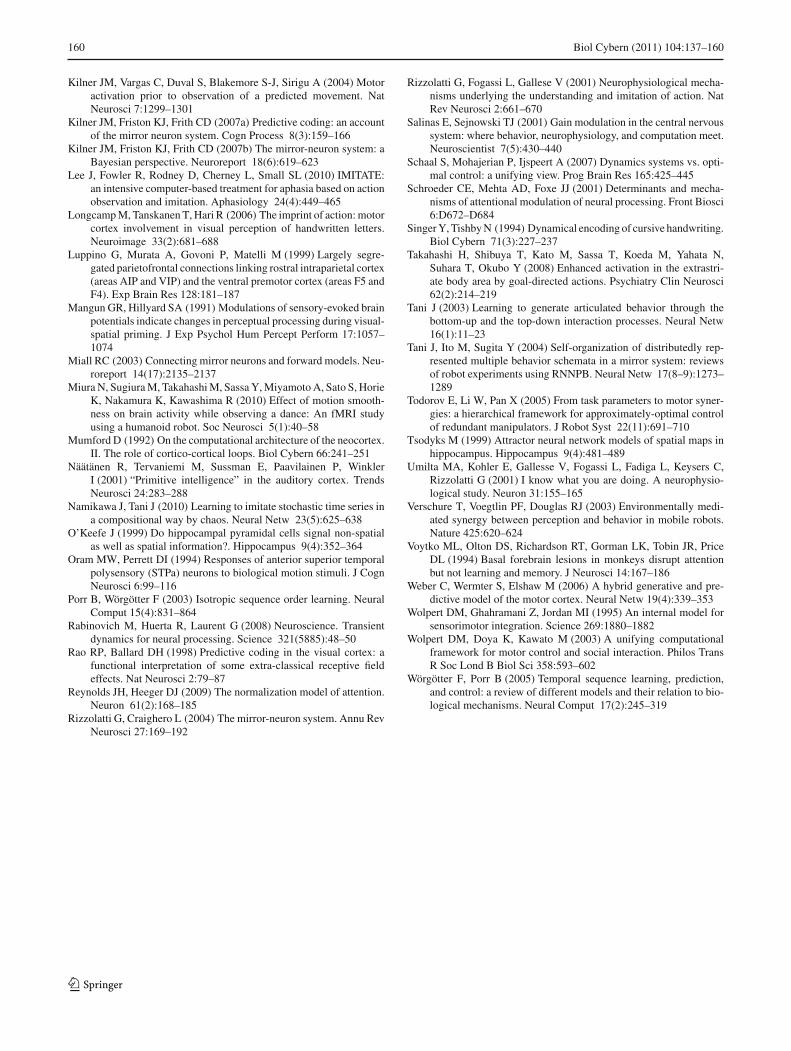
160 Biol Cybern (2011) 104:137–160

Kilner JM, Vargas C, Duval S, Blakemore S-J, Sirigu A (2004) Motoractivation prior to observation of a predicted movement. NatNeurosci 7:1299–1301

Kilner JM, Friston KJ, Frith CD (2007a) Predictive coding: an accountof the mirror neuron system. Cogn Process 8(3):159–166

Kilner JM, Friston KJ, Frith CD (2007b) The mirror-neuron system: aBayesian perspective. Neuroreport 18(6):619–623

Lee J, Fowler R, Rodney D, Cherney L, Small SL (2010) IMITATE:an intensive computer-based treatment for aphasia based on actionobservation and imitation. Aphasiology 24(4):449–465

Longcamp M, Tanskanen T, Hari R (2006) The imprint of action: motorcortex involvement in visual perception of handwritten letters.Neuroimage 33(2):681–688

Luppino G, Murata A, Govoni P, Matelli M (1999) Largely segre-gated parietofrontal connections linking rostral intraparietal cortex(areas AIP and VIP) and the ventral premotor cortex (areas F5 andF4). Exp Brain Res 128:181–187

Mangun GR, Hillyard SA (1991) Modulations of sensory-evoked brainpotentials indicate changes in perceptual processing during visual-spatial priming. J Exp Psychol Hum Percept Perform 17:1057–1074

Miall RC (2003) Connecting mirror neurons and forward models. Neu-roreport 14(17):2135–2137

Miura N, Sugiura M, Takahashi M, Sassa Y, Miyamoto A, Sato S, HorieK, Nakamura K, Kawashima R (2010) Effect of motion smooth-ness on brain activity while observing a dance: An fMRI studyusing a humanoid robot. Soc Neurosci 5(1):40–58

Mumford D (1992) On the computational architecture of the neocortex.II. The role of cortico-cortical loops. Biol Cybern 66:241–251

Näätänen R, Tervaniemi M, Sussman E, Paavilainen P, WinklerI (2001) “Primitive intelligence” in the auditory cortex. TrendsNeurosci 24:283–288

Namikawa J, Tani J (2010) Learning to imitate stochastic time series ina compositional way by chaos. Neural Netw 23(5):625–638

O’Keefe J (1999) Do hippocampal pyramidal cells signal non-spatialas well as spatial information?. Hippocampus 9(4):352–364

Oram MW, Perrett DI (1994) Responses of anterior superior temporalpolysensory (STPa) neurons to biological motion stimuli. J CognNeurosci 6:99–116

Porr B, Wörgötter F (2003) Isotropic sequence order learning. NeuralComput 15(4):831–864

Rabinovich M, Huerta R, Laurent G (2008) Neuroscience. Transientdynamics for neural processing. Science 321(5885):48–50

Rao RP, Ballard DH (1998) Predictive coding in the visual cortex: afunctional interpretation of some extra-classical receptive fieldeffects. Nat Neurosci 2:79–87

Reynolds JH, Heeger DJ (2009) The normalization model of attention.Neuron 61(2):168–185

Rizzolatti G, Craighero L (2004) The mirror-neuron system. Annu RevNeurosci 27:169–192

Rizzolatti G, Fogassi L, Gallese V (2001) Neurophysiological mecha-nisms underlying the understanding and imitation of action. NatRev Neurosci 2:661–670

Salinas E, Sejnowski TJ (2001) Gain modulation in the central nervoussystem: where behavior, neurophysiology, and computation meet.Neuroscientist 7(5):430–440

Schaal S, Mohajerian P, Ijspeert A (2007) Dynamics systems vs. opti-mal control: a unifying view. Prog Brain Res 165:425–445

Schroeder CE, Mehta AD, Foxe JJ (2001) Determinants and mecha-nisms of attentional modulation of neural processing. Front Biosci6:D672–D684

Singer Y, Tishby N (1994) Dynamical encoding of cursive handwriting.Biol Cybern 71(3):227–237

Takahashi H, Shibuya T, Kato M, Sassa T, Koeda M, Yahata N,Suhara T, Okubo Y (2008) Enhanced activation in the extrastri-ate body area by goal-directed actions. Psychiatry Clin Neurosci62(2):214–219

Tani J (2003) Learning to generate articulated behavior through thebottom-up and the top-down interaction processes. Neural Netw16(1):11–23

Tani J, Ito M, Sugita Y (2004) Self-organization of distributedly rep-resented multiple behavior schemata in a mirror system: reviewsof robot experiments using RNNPB. Neural Netw 17(8–9):1273–1289

Todorov E, Li W, Pan X (2005) From task parameters to motor syner-gies: a hierarchical framework for approximately-optimal controlof redundant manipulators. J Robot Syst 22(11):691–710

Tsodyks M (1999) Attractor neural network models of spatial maps inhippocampus. Hippocampus 9(4):481–489

Umilta MA, Kohler E, Gallesse V, Fogassi L, Fadiga L, Keysers C,Rizzolatti G (2001) I know what you are doing. A neurophysio-logical study. Neuron 31:155–165

Verschure T, Voegtlin PF, Douglas RJ (2003) Environmentally medi-ated synergy between perception and behavior in mobile robots.Nature 425:620–624

Voytko ML, Olton DS, Richardson RT, Gorman LK, Tobin JR, PriceDL (1994) Basal forebrain lesions in monkeys disrupt attentionbut not learning and memory. J Neurosci 14:167–186

Weber C, Wermter S, Elshaw M (2006) A hybrid generative and pre-dictive model of the motor cortex. Neural Netw 19(4):339–353

Wolpert DM, Ghahramani Z, Jordan MI (1995) An internal model forsensorimotor integration. Science 269:1880–1882

Wolpert DM, Doya K, Kawato M (2003) A unifying computationalframework for motor control and social interaction. Philos TransR Soc Lond B Biol Sci 358:593–602

Wörgötter F, Porr B (2005) Temporal sequence learning, prediction,and control: a review of different models and their relation to bio-logical mechanisms. Neural Comput 17(2):245–319

123