Action-Reaction: Forecasting the Dynamics of … · Action-Reaction: Forecasting the Dynamics of Human Interaction 3 and action space are extremely large. In this scenario, it is

Action-Reaction:Forecasting the Dynamics of Human Interaction

De-An Huang and Kris M. Kitani

Carnegie Mellon University, Pittsburgh, PA 15213 USA

Abstract. Forecasting human activities from visual evidence is an emerg-ing area of research which aims to allow computational systems to makepredictions about unseen human actions. We explore the task of activityforecasting in the context of dual-agent interactions to understand howthe actions of one person can be used to predict the actions of another.We model dual-agent interactions as an optimal control problem, wherethe actions of the initiating agent induce a cost topology over the spaceof reactive poses – a space in which the reactive agent plans an opti-mal pose trajectory. The technique developed in this work employs akernel-based reinforcement learning approximation of the soft maximumvalue function to deal with the high-dimensional nature of human mo-tion and applies a mean-shift procedure over a continuous cost functionto infer a smooth reaction sequence. Experimental results show that ourproposed method is able to properly model human interactions in a highdimensional space of human poses. When compared to several baselinemodels, results show that our method is able to generate highly plausiblesimulations of human interaction.

1 Introduction

It is our aim to expand the boundaries of human activity analysis by buildingintelligent systems that are not only able to classify human activities but are alsocapable of mentally simulating and extrapolating human behavior. The idea ofpredicting unseen human actions has been studied in several contexts, such asearly detection [17], activity prediction [22], video gap-filling [2], visual prediction[25] and activity forecasting [9]. The ability to predict human activity based on

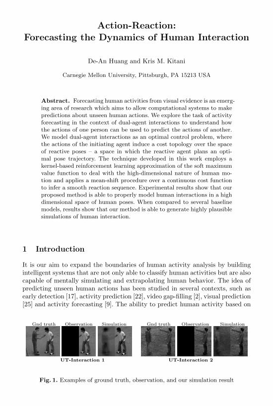
Gnd truth Observation Simulation Gnd truth Observation Simulation

UT-Interaction 1 UT-Interaction 2

Fig. 1. Examples of ground truth, observation, and our simulation result

2 De-An Huang and Kris M. Kitani

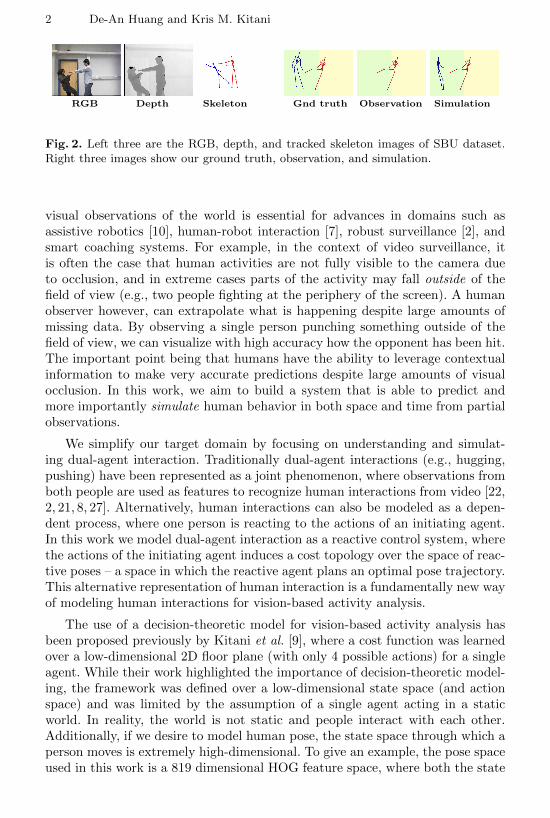
RGB Depth Skeleton Gnd truth Observation Simulation

Fig. 2. Left three are the RGB, depth, and tracked skeleton images of SBU dataset.Right three images show our ground truth, observation, and simulation.

visual observations of the world is essential for advances in domains such asassistive robotics [10], human-robot interaction [7], robust surveillance [2], andsmart coaching systems. For example, in the context of video surveillance, itis often the case that human activities are not fully visible to the camera dueto occlusion, and in extreme cases parts of the activity may fall outside of thefield of view (e.g., two people fighting at the periphery of the screen). A humanobserver however, can extrapolate what is happening despite large amounts ofmissing data. By observing a single person punching something outside of thefield of view, we can visualize with high accuracy how the opponent has been hit.The important point being that humans have the ability to leverage contextualinformation to make very accurate predictions despite large amounts of visualocclusion. In this work, we aim to build a system that is able to predict andmore importantly simulate human behavior in both space and time from partialobservations.

We simplify our target domain by focusing on understanding and simulat-ing dual-agent interaction. Traditionally dual-agent interactions (e.g., hugging,pushing) have been represented as a joint phenomenon, where observations fromboth people are used as features to recognize human interactions from video [22,2, 21, 8, 27]. Alternatively, human interactions can also be modeled as a depen-dent process, where one person is reacting to the actions of an initiating agent.In this work we model dual-agent interaction as a reactive control system, wherethe actions of the initiating agent induces a cost topology over the space of reac-tive poses – a space in which the reactive agent plans an optimal pose trajectory.This alternative representation of human interaction is a fundamentally new wayof modeling human interactions for vision-based activity analysis.

The use of a decision-theoretic model for vision-based activity analysis hasbeen proposed previously by Kitani et al. [9], where a cost function was learnedover a low-dimensional 2D floor plane (with only 4 possible actions) for a singleagent. While their work highlighted the importance of decision-theoretic model-ing, the framework was defined over a low-dimensional state space (and actionspace) and was limited by the assumption of a single agent acting in a staticworld. In reality, the world is not static and people interact with each other.Additionally, if we desire to model human pose, the state space through which aperson moves is extremely high-dimensional. To give an example, the pose spaceused in this work is a 819 dimensional HOG feature space, where both the state

Action-Reaction: Forecasting the Dynamics of Human Interaction 3

and action space are extremely large. In this scenario, it is no longer feasible touse the discrete state inference procedure used in [9].

In this work, we aim to go beyond a two dimensional state space and forecastdual-agent activities in a high-dimensional pose space. In particular, we intro-duce kernel-based reinforcement learning [18] to handle the high-dimensionalityof human pose. Furthermore, we introduce an efficient mean-shift inference pro-cedure [4] to find an optimal pose trajectory in the continuous cost functionspace. In comparative experiments, the results verify that our inference methodis able to effectively represent human interactions. Furthermore, we show howthis procedure proposed for 2D dual-agent interaction forecasting can also be ap-plied to 3D skeleton pose data. Our final qualitative experiment also shows howthe proposed model can be used for human pose analysis and anomaly detection.

Interestingly, the idea of generating a reactive pose trajectory has been ex-plored largely in computer graphics; a problem known as interactive control. Thegoal of interactive control is to create avatar animations in response to user in-put [12, 15]. Motion graphs [11] created from human motion data are commonlyused, and the motion synthesis problem is transformed into selecting proper se-quences of nodes. However, these graphs are discrete and obscure the continuousproperties of motion. In response, a number of approaches have been proposedto alleviate this weakness and perform continuous control of character [24, 13,14]. It should be noted that all of the interactive control approaches focus onsynthesizing animations in response to a clearly defined mapping [11, 15] fromthe user input to pose. In contrast, we aim to simulate human reaction basedonly on visual observations, where the proper reaction is non-obvious and mustbe learned from the data.

2 Dual Agent Forecasting

Our goal is to build a system that can simulate human reaction based only onvisual observations. As shown in Figure 1, the ground truth consists of both thetrue reaction g = [g1 · · · gT ] on the left hand side (LHS) and the observationo = [o1 · · · oT ] of the initiating agent on the right hand side (RHS). In trainingtime, M demonstrated interaction pairs gm and om are provided for us to learnthe cost topology of human interaction. At test time, only the actions of theinitiating agent o (observation) on the RHS is given. We perform inference overthe learned cost function to obtain an optimal reaction sequence x.

2.1 Markov Decision Processes

In this work, we model dual-agent interaction as a Markov decision process(MDP) [1]. At each time step, the process is in some state c, and the agent maychoose any action a that is available in state c. The process responds by movingto a new state c′ at the next time step. The MDP is defined by an initial statedistribution p0(c) a transition model p(c′|c, a) and a reward function r(c, a),which is equivalent to the negative cost function. Given these parameters, the


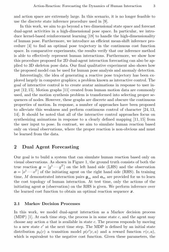
(a) Input image (b) Foreground map (c) HOG

Fig. 3. HOG features in (c) are our 819 dimensional states, which are the HOG re-sponses of the input images weighted by the probability of foreground maps in (b).

goal of optimal control is to learn the optimal policy π(a|c), which encodes thedistribution of action a to take when in state c that can maximize the expectedreward (minimize the expected cost). In this work, the actions are deterministicbecause we assume humans have perfect control over their body where one ac-tion will deterministically bring the pose to the next state. Therefore, p(c′|c, a)concentrates on a single state c′ = ca and is zero for other states.

2.2 States and Actions

States. We use a HOG [6] feature of the whole image as a compact state repre-sentation, which does not contain the redundant textural information in the rawimages. Some visualizations are shown in Figure 3. Note that only the poses onthe left hand side (LHS) are referred as states, while poses on the right hand side(RHS) are our observations. We further make two changes to adapt HOG featureto our current application, pose representation. First, the HOG is weighted byprobability of foreground (PFG) of the corresponding image because we are onlyinterested in the human in the foreground. The PFG is computed by median fil-tering followed by soft thresholding. Second, we average the gradient in the 2×2overlapping cells in HOG to reduce its dimension. This results in a continuoushigh-dimensional vector of 819 dimensions (64× 112 bounding box).

Actions. Even with a continuous state space, a discrete set of actions isstill more efficient to solve the MDP when possible [14]. Furthermore, there areactually many redundant actions for similar states that can be removed [23]. Toalleviate redundancy, we perform k-means clustering on all the training frameson the LHS to quantize the continuous state space into K discrete states. Foreach cluster c (c = 1 to K), we will refer to the cluster center Xc as the HOGfeature of quantized state c. The kth action is defined as going from a quantizedstate c to the kth nearest state, which gives us a total K actions. In the rest ofthe paper, we will fix this quantization. Given a new pose vector (HOG feature)x on the LHS, it is quantized to state c if Xc is the closest HOG feature to x.

2.3 Inverse Optimal Control over Quantized State Space

In this work, we model dual-agent interaction as an optimal control problem,where the actions of the initiating agent induce a cost topology over the space


of reactive poses. Given M demonstrated interaction pair om (Observation) andgm (true reaction), we leverage recent progress in inverse optimal control (IOC)[28] to recover a discretized approximation of the underlying cost topology.

In contrast to optimal control in Section 2.1, the cost function is not givenin IOC and has to be derived from demonstrated examples [16]. We make animportant assumption about the form of the cost function, which enables us totranslate from visual observations to a single cost for reactive poses. The reward(negative cost) of a state c and an action a:

r(c, a;θ) = θ>f(c, a), (1)

is assumed to be a weighted combination of feature responses f(c, a) =[f1(c, a) · · · fJ(c, a)]>, where each fj(c, a) is the response of a type of featureextracted from the video, such as the velocity of the agent’s center of mass, andθ is a vector of weights for each feature. By learning these parameters θ, we arelearning how the actions of the initiating agent affect the reaction of the partner.For example, a feature such as moving forward will have a high cost for punchinginteractions because moving forward increases the possibility of being hit by thepunch. In this case, the punching activity induces a high cost on moving forwardand implies that this feature should have a high weight in the cost function. Thisexplicit modeling of human interaction dynamics via the cost function sets ourapproach apart from traditional human interaction recognition models.

In this work, we apply the maximum entropy IOC approach [28] on thequantized states to learn a discretized approximation of the cost function. In thiscase, for a pose sequence x = [x1 · · ·xT ] on the LHS, we quantize it into sequencec = [c1 · · · cT ] of quantized states defined in Section 2.2. In the maximum entropyframework [28], the distribution over a sequence c of quantized states and thecorresponding sequence a of actions is defined as:

P (c,a;θ) =

∏t er(ct,at)

Z(θ)=e∑t θ>f (ct,at)

Z(θ), (2)

where θ are the weights of the cost function, f(ct, at) is the corresponding vectorof features of state ct and action at, and Z(θ) is the partition function.

In the training step, we quantize M training pose sequences g1 · · · gM onthe LHS to get the corresponding sequences c1 · · · cM of quantized states. Wethen recover the reward function parameters θ by maximizing the likelihoodof these sequences under the maximum entropy distribution (2). We use expo-nentiated gradient descent to iteratively maximize the likelihood. The gradientcan be shown to be the difference between the empirical mean feature countf̄ = 1

M

∑Mm=1 f(cm,am), the average feature counts over the demonstrated

training sequences, and the expected mean feature count f̂θ, the average fea-ture counts over the sequences generated by the parameter θ. With step size

η, we update θ by θt+1 = θteη(f̄−f̂θ). In order to compute the expected featurecount f̂θ, we use a two-step algorithm similar to that described in [9] and [28].


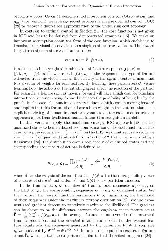
Algorithm 1 – Backwards pass

V (T )(c)← 0for t = T − 1, . . . , 2, 1 do

V (t)(c) = soft maxa r(c, a; θ) + V (t+1)(ca)

π(t)θ (a|c) ∝ eV

(t)(ca)−V (t)(c)

end for

Algorithm 2 – Forward pass

D(1)(c)← 1K

for t = 1, 2, . . . , T − 1 do

D(t+1)(ca) += π(t)θ (a|c)D(t)(c)

end forf̂θ =

∑t

∑c

∑a f

(t)(c, a)D(t)(c)

Backward pass. In the first step, current weight parameters θ is used tocompute the expected reward V (t)(c) to the goal from any possible state c atany time step t. The expected reward function V (t)(c) is also called the value

function in reinforcement learning. The maximum entropy policy is π(t)θ (a|c) ∝

eV(t)(ca)−V (t)(c), where c is the current state, a is an action, and ca is the state

we will get by performing action a at state c. In other words, the probabilityof going to a state ca from c is exponentially proportional to the increase ofexpected reward or value. The algorithm is summarized in Algorithm 1.

Forward pass. In the second step, we propagate an uniform initial distribution

p0(c) = 1K according to the learned policy π

(t)θ (a|c), where K is the number

of states (clusters). We do not assume c1 is known as in [9] and [28]. In thiscase, we can compute the expected state visitation count D(t)(c) of state c attime step t. Therefore, the expected mean feature count can be computed byf̂θ =

∑t

∑c

∑a f

(t)(c, a)D(t)(c). The algorithm is summarized in Algorithm 2.

2.4 Features for Human Interaction

According to (1), the features define the expressiveness of our cost function andare crucial to our method in modeling dynamics of human interaction. Now wedescribe the features we use in our method. In this work, we assume that thepose sequence o = [o1 · · · oT ] of the initiating agent is observable on the RHS.

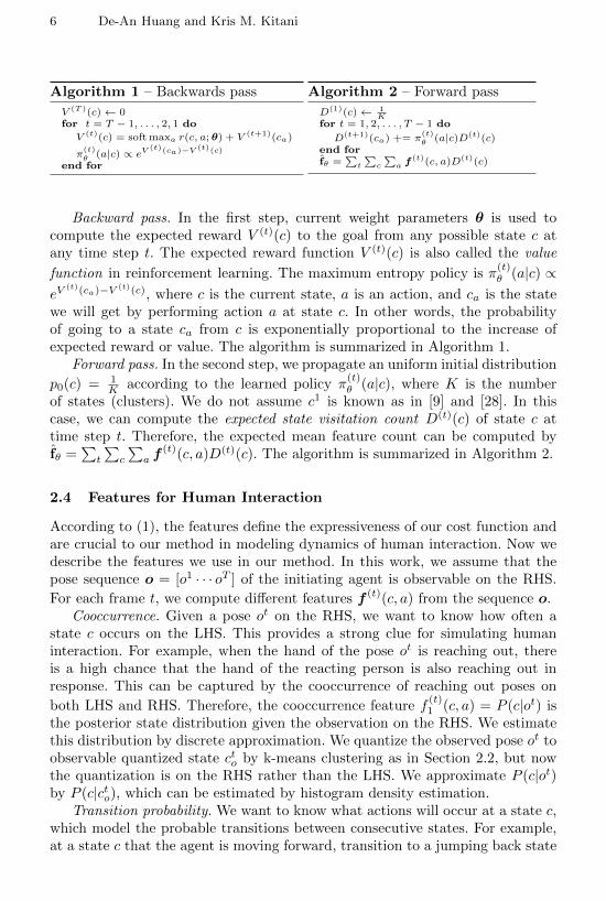
For each frame t, we compute different features f (t)(c, a) from the sequence o.Cooccurrence. Given a pose ot on the RHS, we want to know how often a

state c occurs on the LHS. This provides a strong clue for simulating humaninteraction. For example, when the hand of the pose ot is reaching out, thereis a high chance that the hand of the reacting person is also reaching out inresponse. This can be captured by the cooccurrence of reaching out poses on

both LHS and RHS. Therefore, the cooccurrence feature f(t)1 (c, a) = P (c|ot) is

the posterior state distribution given the observation on the RHS. We estimatethis distribution by discrete approximation. We quantize the observed pose ot toobservable quantized state cto by k-means clustering as in Section 2.2, but nowthe quantization is on the RHS rather than the LHS. We approximate P (c|ot)by P (c|cto), which can be estimated by histogram density estimation.

Transition probability. We want to know what actions will occur at a state c,which model the probable transitions between consecutive states. For example,at a state c that the agent is moving forward, transition to a jumping back state


likely unlikely smooth abrupt attraction repulsion

Cooccurence Transition Symmetry

Fig. 4. We use statistics of human interaction as our features for the cost function.

is less likely. Therefore, the second feature is the transition probability f(t)2 (c, a)

= P (ca|c), where ca is the state we will get to by performing action a at statec. We accumulate the transition statistics from the M training sequences cm ofquantized states on the LHS. This feature is independent of time step t.

Centroid velocity. We use centroid velocities to capture the movements ofpeople when they are interacting. For example, it is unlikely that the centroid po-sition of human will move drastically across frames and actions that induce highcentroid velocity should be penalized. Therefore, we define the feature smooth-

ness as f(t)3 (c, a) = 1 − σ(|v(c, a)|), where σ(·) is the sigmoid function, and

v(c, a) is the centroid velocity of action a at state c. Only the velocity along thex-axis is used. In addition, the relative velocity of the interacting agents givesus information about the current interaction. For example, in the hugging ac-tivity, the interacting agents are approaching each other and will have centroidvelocities of opposite directions. Therefore, we define the feature attraction as

f(t)4 (c, a) = 1(vto × v(c, a) < 0), where 1(·) is the indicator function, and vto is

the centroid velocity of the initiating agent at time t. This feature will be one ifthe interacting agents are moving in a symmetric way. We also define the com-

plementary feature repulsion as f(t)5 (c, a) = 1(vto × v(c, a) > 0) to capture the

opposite case when the agents are repulsive to each other.

2.5 Quantized State Inference

Given a set of demonstrated interactions, we can learn a discretized approxima-tion of the underlying cost function by the IOC algorithm presented in Section2.3. At test time, only the pose sequence of the initiating agent otest on the RHSis observable. We first compute the features f (t)(c, a) under the observation otest,and weight the features by the learned weight parameters θ to get the rewardfunction (negative cost) r(c, a;θ) = θ>f(c, a). This gives us the approximatedcost topology induced by otest, the pose sequence of the initiating agent.

In discrete Markov decision process, inferring the most probable sequence isstraightforward: First, we fix the induced r(c, a;θ) and perform one round ofbackwards pass (Algorithm 1) to get the discrete value function V (t)(c). At eachtime step t, the most probable state is the state with the highest value. However,the result depends highly on the selection of K in this case. If we choose K toolarge, the O(K2T ) Algorithm 1 becomes computational prohibited. Furthermore,the histogram based estimations become unreliable. On the other hand, if wechoose K too small, the quantization error can be large.


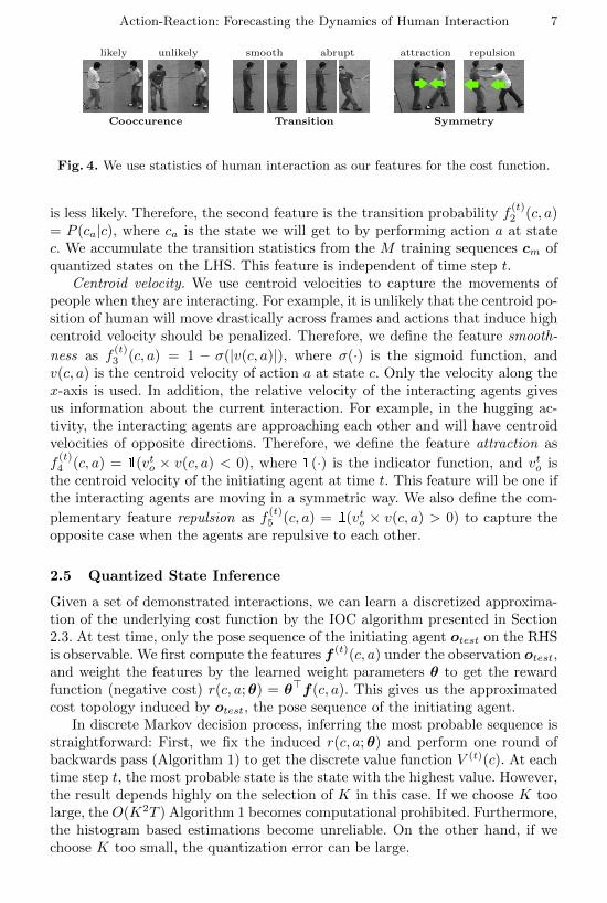
Algorithm 3 – Extended Mean Shift Inference

Compute V (t)(c) by Algorithm 1

x1 = Xc∗ , where c∗ = arg maxc V(1)(c)

for t = 2, . . . , T do

x0 = xt−1, wc = V (t)(c)while not converged doxi+1 = 1

Ch

∑Kc=1XcwcKh(xi, Xc), where Ch =

∑Kc=1 wcKh(xi, Xc)

end whilext = xconverged

end for

2.6 Kernel-based Reinforcement Learning

In order to address the problems of discretizing the state space, we introducekernel-based reinforcement learning (KRL) [18] to our problem. Based on KRL,

the value function V(t)h (x) for any pose x in the continuous state space is assumed

to be a weighted combination of value functions V (t)(c) of the quantized states.This translate our inference from discrete to continuous state space. At eachtime step t, the value function of a continuous state x is:

V(t)h (x) =

∑Kc=1Kh(x,Xc)V

(t)(c)∑Kc=1Kh(x,Xc)

, (3)

where Xc is the HOG feature of the quantized state c, and Kh(·, ·) is a kernelfunction with bandwidth h. In this work, we use the normal kernel.

The advantage of KRL is two-fold. First, it guarantees the smoothness ofour value function. Second, we have the value function on the continuous space.Therefore, even with smaller K, we can still perform continuous inference. Fur-thermore, this formulation allows us to perform efficient optimization for x with

maximal V(t)h (x) as we will show in the next section.

2.7 Extended Mean Shift Inference

Now that we have the value function V(t)h (x) on the continuous state space, we

want to find the pose x∗ with the highest value. In contrast to optimization inthe discretized space, it is infeasible to enumerate the values of all the statesin continuous space. We leverage the property of human motion to simplify theoptimization problem. Since human motion is smooth and will not change drasti-cally across frames, the optimal next pose should appear in a local neighborhoodof the current pose. This restricts our search space of optimal pose to a localneighborhood. In addition, we leverage the resemblance of our formulation in(3) to the well-studied kernel density estimation (KDE) in statistics, which hasalso achieved considerable success in the area of object tracking [3]. To optimizethe density in KDE, the standard approach is to apply the mean shift proce-dure, which will converge robustly to the local maximum of the density function.


Our formulation allows us to leverage the similarity of our problem to KDE andapply the extended mean shift framework proposed in [3] to perform efficientinference. As shown in [3], the maximization of a function of the form∑K

c=1 wcKh(x,Xc)∑Kc=1Kh(x,Xc)

(4)

can be done efficiently by the extended mean shift iterations

xi+1 =

∑Kc=1XcwcGh(xi, Xc)∑Kc=1 wcGh(xi, Xc)

(5)

until convergence, where Gh is the negative gradient of Kh. In normal kernel,Gh and Kh has the same form [4]. Therefore, we can replace Gh in (5) by Kh.

Our goal is to find the pose x that maximize the value function V(t)h (x)

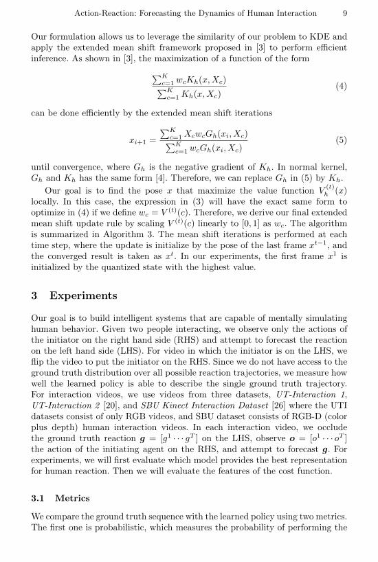
locally. In this case, the expression in (3) will have the exact same form tooptimize in (4) if we define wc = V (t)(c). Therefore, we derive our final extendedmean shift update rule by scaling V (t)(c) linearly to [0, 1] as wc. The algorithmis summarized in Algorithm 3. The mean shift iterations is performed at eachtime step, where the update is initialize by the pose of the last frame xt−1, andthe converged result is taken as xt. In our experiments, the first frame x1 isinitialized by the quantized state with the highest value.

3 Experiments

Our goal is to build intelligent systems that are capable of mentally simulatinghuman behavior. Given two people interacting, we observe only the actions ofthe initiator on the right hand side (RHS) and attempt to forecast the reactionon the left hand side (LHS). For video in which the initiator is on the LHS, weflip the video to put the initiator on the RHS. Since we do not have access to theground truth distribution over all possible reaction trajectories, we measure howwell the learned policy is able to describe the single ground truth trajectory.For interaction videos, we use videos from three datasets, UT-Interaction 1,UT-Interaction 2 [20], and SBU Kinect Interaction Dataset [26] where the UTIdatasets consist of only RGB videos, and SBU dataset consists of RGB-D (colorplus depth) human interaction videos. In each interaction video, we occludethe ground truth reaction g = [g1 · · · gT ] on the LHS, observe o = [o1 · · · oT ]the action of the initiating agent on the RHS, and attempt to forecast g. Forexperiments, we will first evaluate which model provides the best representationfor human reaction. Then we will evaluate the features of the cost function.

3.1 Metrics

We compare the ground truth sequence with the learned policy using two metrics.The first one is probabilistic, which measures the probability of performing the


ground truth reaction under the learned policy. A higher probability means thelearned policy is more consistent with the ground truth reaction sequence. Weuse the Negative Log-Likelihood (NLL):

− logP (g|o) = −∑t

logP (gt|gt−1,o), (6)

as our probabilistic metric. For discrete models, the ground truth reaction se-quence is quantized into a sequence c of quantized states. The probability is eval-uated by P (gt|gt−1,o) = P (ct|ct−1,o). For our continuous model, P (gt|gt−1,o)are interpolated according to (3). The second metric is deterministic, which di-rectly measure the physical HOG distance (or joint distance for skeleton video)of the ground truth reaction g and the reaction simulated by the learned policy.The deterministic metric is the average frame distance:

1

T − 1

∑t

||gt − xt||2 (7)

where xt is the resulting reaction pose at frame t. The distance is not computedfor the last frame because the reward function r(c, a) is not defined.

3.2 Evaluating the Interaction Model

For model evaluation, we select three baselines to compare with the proposedmethod. The first baseline is the per frame nearest neighbor (NN) [5], whichonly uses the cooccurrence feature at each frame independently and does nottake into account the effect of consecutive states. For each observation ot, wefind the LHS quantized state with the highest cooccurrence. That is ctNN =arg maxc P (c|cto) ≈ P (c|ot), where cto is the observable quantized state of ot.

The second baseline is the hidden Markov model (HMM) [19], which has beenwidely used to recover hidden time sequences. HMM is defined by the transitionprobabilities P (ct|ct−1) and emission probabilities P (ot|ct), which are equivalentto our transition and cooccurrence features. However, the weights for these twofeatures are always the same in HMM, while our algorithm learns the optimalfeature weights θ. The likelihood is computed by the forward algorithm and theresulting state sequence cHMM is computed by the Viterbi algorithm.

Table 1. Average frame distance (AFD) and NLL per activity category for UTI

(a)AFD NN[5] HMM[19] MDP[9] Proposedshake 5.35 5.21 4.68 3.14hug 4.00 4.06 3.74 2.88kick 6.17 6.16 5.33 3.96point 3.62 3.62 3.31 2.45punch 5.10 4.99 4.23 3.03push 4.90 4.91 4.01 3.24

(b)NLL NN[5] HMM[19] MDP[9] Proposedshake 651.04 473.91 862.81 476.10hug 751.46 608.81 958.49 487.21kick 382.62 263.08 550.52 282.36point 577.22 426.40 750.11 374.73punch 353.85 260.72 483.01 257.06push 479.33 357.00 561.01 320.92


t = 20 t = 30 t = 40 t = 50 t = 60

t = 70 t = 80 t = 90 t = 100 t = 110

Fig. 5. Forecasting result of UTI dataset 1. The RHS is the observed initiator, and theLHS is the simulated reaction of the proposed method. The activity is shaking hands.

t = 20 t = 30 t = 40 t = 50 t = 60

t = 70 t = 80 t = 90 t = 100 t = 110

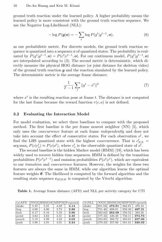
Fig. 6. Forecasting result of UTI dataset 2. The RHS is the observed initiator, and theLHS is the simulated reaction of the proposed method. The activity is hugging.

The third baseline is the discrete state inference in Section 2.5. This canbe seen as applying the discrete Markov decision process (MDP) inference usedin [9] to a quantized state space. We will refer to this baseline as MDP. The

likelihood for MDP is computed by∏t π

(t)θ (at|ct), the stepwise product of the

policy executions. We follow [9] and produce the probabilistic-weighted output.We first evaluate our method on UT-Interaction 1, and UT-Interaction 2

[20] datasets, which consist of RGB videos only, and some examples have beenshown in Figure 1. The UTI datsets consist of 6 actions: hand shaking, hugging,kicking, pointing, punching, pushing. Each action has a total of 10 sequencesfor both datasets. We use 10-fold evaluation as in [2]. We use K = 100 in theexperiments. We now evaluate which method can best simulate human reaction.

The average NLL and frame distance per activity for each baseline is shown inTable 1. It can be seen that, optimal control based methods (MDP and proposed)outperform the other two baselines in terms of frame distance. In addition, theproposed mean shift inference achieves the lowest frame distance for all activitiesand significantly outperforms other baselines because we use kernel-based rein-forcement learning to alleviate quantization error and the mean shift inferenceensures the smoothness of the resulting reaction trajectory. It should be notedthat although the MDP is able to achieve lower frame distance than NN andHMM, the NLL is higher. This is because the performance of discretized infer-ence can be affected significantly by unseen data. For example, if a transition is


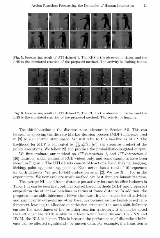
Fig. 7. Ablative analysis shows that the proposed method continually outperforms thebaselines and verifies the effectiveness of our features.

not observed in the training data, it will generate a low transition probabilityfeature and induce a high cost in the IOC framework. This will make the overalllikelihood of the ground truth significantly lower (a high NLL). On the otherhand, our kernel-based reinforcement learning framework interpolates a smoothvalue function over the continuous state space and alleviates this phenomenon.The effectiveness of our approach is verified by the NLL shown in Table 1. Somevisualization of the results are shown in Figure 5 and Figure 6.

3.3 Evaluating the Effect of Features

As noted in Section 2.4, the features define the expressiveness of our cost func-tion, and are essential for us to model the dynamics of human interaction. In theprevious section, we have shown that the proposed method is the best interactionmodel. We now evaluate the effects of different features for our model.

The average NLL and frame distance for the entire UTI dataset (1 and 2)using different features are shown in Figure 7. The performances of baselinesand MDP are also shown for reference. It should be note that because centroid-based features (smooth, attraction, repulsion) cannot be easily integrated intobaselines NN and HMM, the performances of HMM still only use the first twofeatures in the +Smooth and +Symmetry columns. It can be seen that addingmore features help our method to learn a policy that is more consistent with theground truth, and significantly outperforms other baselines because our kernel-based reinforcment learning and mean-shift framework provides an efficient wayfor inference over a continuous space and ensures the smoothness of the result.

3.4 Extension to 3D Pose Space

To show that our method can also work in 3D pose space (not just 2D), we eval-uate our method on SBU Kinect Interaction Dataset [26], in which interactionsperformed by two people are captured by a RGB-D sensor and tracked skeletonpositions at each frame are provided. In this case, the state space becomes a 15×3(joint number times x, y, z) dimensional continuous vector. We use K = 50 forthe actions because the dataset contains less frames per video compared to theUT-Interaction datasets. The SBU dataset consists of 8 actions: approaching, de-parting, kicking,pushing, shaking hands, hugging, exchanging object, punching.


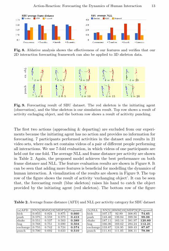
Fig. 8. Ablative analysis shows the effectiveness of our features and verifies that our2D interaction forecasting framework can also be applied to 3D skeleton data.

ex.

ob

j.

t = 0 t = 5 t = 10 t = 15 t = 20

punch

t = 0 t = 5 t = 10 t = 15 t = 20

Fig. 9. Forecasting result of SBU dataset. The red skeleton is the initiating agent(observation), and the blue skeleton is our simulation result. Top row shows a result ofactivity exchaging object, and the bottom row shows a result of acitivity punching.

The first two actions (approaching & departing) are excluded from our experi-ments because the initiating agent has no action and provides no information forforecasting. 7 participants performed activities in the dataset and results in 21video sets, where each set contains videos of a pair of different people performingall interactions. We use 7-fold evaluation, in which videos of one participants areheld out for one fold. The average NLL and frame distance per activity are shownin Table 2. Again, the proposed model achieves the best performance on bothframe distance and NLL. The feature evaluation results are shown in Figure 8. Itcan be seen that adding more features is beneficial for modelling the dynamics ofhuman interaction. A visualization of the results are shown in Figure 9. The toprow of the figure shows the result of activity ‘exchanging object’. It can be seenthat, the forecasting result (blue skeleton) raises his hand to catch the objectprovided by the initiating agent (red skeleton). The bottom row of the figure

Table 2. Average frame distance (AFD) and NLL per activity category for SBU dataset

(a)AFD NN[5] HMM[19] MDP[9] Proposedkick 0.855 0.824 0.875 0.660push 0.575 0.559 0.573 0.413shake 0.551 0.537 0.503 0.389hug 0.768 0.751 0.690 0.504exchange 0.755 0.742 0.724 0.574punch 0.700 0.692 0.633 0.510

(b)NLL NN[5] HMM[19] MDP[9] Proposedkick 107.17 92.89 308.85 74.65push 143.46 139.84 399.56 99.06shake 187.11 183.14 381.97 120.89hug 166.06 169.62 284.24 112.21exchange 133.87 124.95 309.43 87.87punch 111.81 111.05 306.11 78.98


forw

ard

t = 0 t = 15 t = 25 t = 35 t = 44

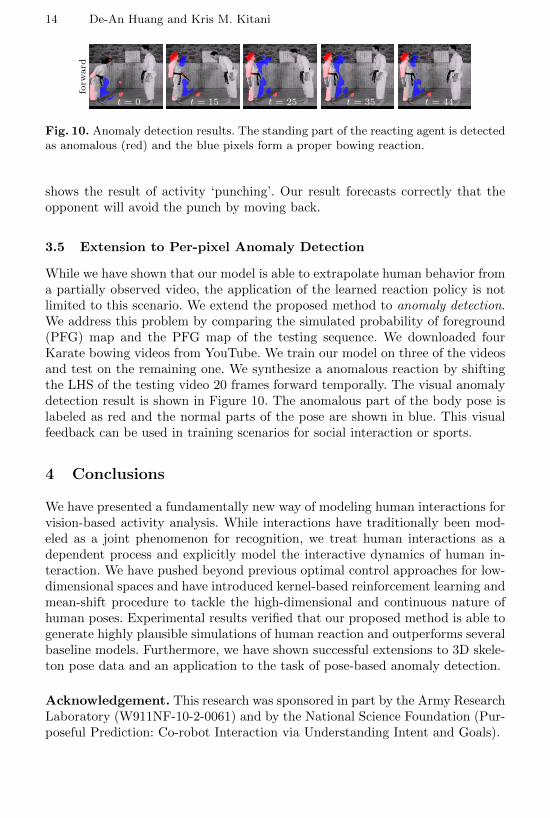
Fig. 10. Anomaly detection results. The standing part of the reacting agent is detectedas anomalous (red) and the blue pixels form a proper bowing reaction.

shows the result of activity ‘punching’. Our result forecasts correctly that theopponent will avoid the punch by moving back.

3.5 Extension to Per-pixel Anomaly Detection

While we have shown that our model is able to extrapolate human behavior froma partially observed video, the application of the learned reaction policy is notlimited to this scenario. We extend the proposed method to anomaly detection.We address this problem by comparing the simulated probability of foreground(PFG) map and the PFG map of the testing sequence. We downloaded fourKarate bowing videos from YouTube. We train our model on three of the videosand test on the remaining one. We synthesize a anomalous reaction by shiftingthe LHS of the testing video 20 frames forward temporally. The visual anomalydetection result is shown in Figure 10. The anomalous part of the body pose islabeled as red and the normal parts of the pose are shown in blue. This visualfeedback can be used in training scenarios for social interaction or sports.

4 Conclusions

We have presented a fundamentally new way of modeling human interactions forvision-based activity analysis. While interactions have traditionally been mod-eled as a joint phenomenon for recognition, we treat human interactions as adependent process and explicitly model the interactive dynamics of human in-teraction. We have pushed beyond previous optimal control approaches for low-dimensional spaces and have introduced kernel-based reinforcement learning andmean-shift procedure to tackle the high-dimensional and continuous nature ofhuman poses. Experimental results verified that our proposed method is able togenerate highly plausible simulations of human reaction and outperforms severalbaseline models. Furthermore, we have shown successful extensions to 3D skele-ton pose data and an application to the task of pose-based anomaly detection.

Acknowledgement. This research was sponsored in part by the Army ResearchLaboratory (W911NF-10-2-0061) and by the National Science Foundation (Pur-poseful Prediction: Co-robot Interaction via Understanding Intent and Goals).


References

1. Bellman, R.: A Markovian decision process. Journal of Mathematics and Mechanics6(5), 679–684 (1957)

2. Cao, Y., Barrett, D.P., Barbu, A., Narayanaswamy, S., Yu, H., Michaux, A., Lin,Y., Dickinson, S.J., Siskind, J.M., Wang, S.: Recognize human activities from par-tially observed videos. In: CVPR (2013)

3. Comaniciu, D., Ramesh, V., Meer, P.: Real-time tracking of non-rigid objects usingmean shift. In: CVPR (2000)

4. Comaniciu, D., Meer, P.: Mean shift: A robust approach toward feature spaceanalysis. IEEE Trans. Pattern Anal. Mach. Intell 24(5), 603–619 (2002)

5. Cover, T.M., Hart, P.E.: Nearest neighbor pattern classification. IEEE Transac-tions in Information Theory IT-13(1), 21–27 (1967)

6. Dalal, N., Triggs, B.: Histograms of oriented gradients for human detection. In:CVPR (2005)

7. Dragan, A.D., Lee, K.C.T., Srinivasa, S.S.: Legibility and predictability of robotmotion. In: ACM/IEEE International Conference on Human-Robot Interaction(2013)

8. Gaur, U., Zhu, Y., Song, B., Chowdhury, A.K.R.: A ”string of feature graphs”model for recognition of complex activities in natural videos. In: ICCV (2011)

9. Kitani, K.M., Ziebart, B.D., Bagnell, J.A., Hebert, M.: Activity forecasting. In:ECCV (2012)

10. Koppula, H.S., Saxena, A.: Anticipating human activities using object affordancesfor reactive robotic response. In: RSS (2013)

11. Kovar, L., Gleicher, M., Pighin, F.: Motion graphs. In: SIGGRAPH 2002 Con-ference Proceedings. pp. 473–482. Annual Conference Series, ACM Press/ACMSIGGRAPH (2002)

12. Lee, J., Chai, J., Reitsma, P.S.A., Hodgins, J.K., Pollard, N.S.: Interactive controlof avatars animated with human motion data. ACM Trans. Graph 21(3), 491–500(2002)

13. Lee, Y., Wampler, K., Bernstein, G., Popovic, J., Popovic, Z.: Motion fields forinteractive character locomotion. ACM Trans. Graph 29(6), 138 (2010)

14. Levine, S., Wang, J.M., Haraux, A., Popovic, Z., Koltun, V.: Continuous charactercontrol with low-dimensional embeddings. ACM Trans. Graph 31(4), 28 (2012)

15. McCann, J., Pollard, N.S.: Responsive characters from motion fragments. ACMTrans. Graph 26(3), 6 (2007)

16. Ng, A.Y., Russell, S.: Algorithms for inverse reinforcement learning. In: ICML(2000)

17. Nguyen, M.H., la Torre, F.D.: Max-margin early event detectors. In: CVPR (2012)18. Ormoneit, D., Sen, S.: Kernel based reinforcement learning. Machine Learning

49(2-3), 161–178 (2002)19. Rabiner, L.R., Juang, B.H.: An introduction to hidden Markov models. ASSP

Magazine (1986)20. Ryoo, M.S., Aggarwal, J.K.: UT-Interaction Dataset, ICPR con-

test on Semantic Description of Human Activities (SDHA).http://cvrc.ece.utexas.edu/SDHA2010/Human Interaction.html (2010)

21. Ryoo, M.S., Aggarwal, J.K.: Spatio-temporal relationship match: Video structurecomparison for recognition of complex human activities. In: ICCV (2009)

22. Ryoo, M.: Human activity prediction: Early recognition of ongoing activities fromstreaming videos. In: ICCV (2011)


23. Safonova, A., Hodgins, J.K.: Construction and optimal search of interpolated mo-tion graphs. ACM Trans. Graph 26(3), 106 (2007)

24. Treuille, A., Lee, Y., Popovic, Z.: Near-optimal character animation with continu-ous control. ACM Trans. Graph 26(3), 7 (2007)

25. Walker, J., Gupta, A., Hebert, M.: Patch to the future: Unsupervised visual pre-diction. In: CVPR (2014)

26. Yun, K., Honorio, J., Chattopadhyay, D., Berg, T.L., Samaras, D.: Two-personinteraction detection using body-pose features and multiple instance learning. In:CVPRW (2012)

27. Zhang, Y., 0002, X.L., Chang, M.C., Ge, W., Chen, T.: Spatio-temporal phrasesfor activity recognition. In: ECCV (2012)

28. Ziebart, B., Maas, A., Bagnell, J., Dey, A.: Maximum entropy inverse reinforcementlearning. In: AAAI (2008)

Documents

Action-Reaction: Forecasting the Dynamics of … · Action-Reaction: Forecasting the Dynamics of Human Interaction 3 and action space are extremely large. In this scenario, it is