Embed Size (px)
Citation preview

Abstract
We extend the local-to-zero analysis of models with weak instruments to models
with estimated instruments and regressors and with higher-order dependence between
instruments and disturbances. This framework is applicable to linear models with
expectation variables that are estimated non-parametrically such as the risk-return
trade-off in finance and the impact of inflation uncertainty on real economic activity.
Our simulation evidence suggests that Lagrange Multiplier (LM) confidence intervals
have better coverage in these models. We apply these methods to excess returns on
the S&P 500 index, yen-dollar spot returns, and excess holding yields between 6-month
and 3-month Treasury bills.
JEL classification: C22, C32, G12
Semi-Parametric Weak Instrument Regressions with
an Application to the Risk-Return Trade-off∗
Benoit Perron†
This version: February 2002
∗Thanks go to two referees, the Editor, Peter Phillips, Oliver Linton, Donald Andrews, Hyungsik Moon,
John Galbraith and seminar participants at Yale, Toronto, Montréal, Concordia, Rutgers, Windsor, Florida
International University, and the 2000 World Congress of the Econometric Society for helpful comments
and suggestions. The usual disclaimer necessarily applies. Financial assistance from the Alfred P. Sloan
Foundation, the Social Science Research Council of Canada, the Fonds pour la Formation des chercheurs
et l’aide à la recherche (FCAR), and the Mathematics of Information Technology and Complex Systems
(MITACS) network is gratefully acknowledged.†Département de sciences économiques and CRDE, Université de Montréal, C.P. 6128, Succursale Centre-
ville, Montréal (Québec), H3C 3J7. E-mail: [email protected].
1. Introduction
Recently, the problem of weak correlation between instruments and regressors in instrumental
variable (IV) regressions has become a focal point of much research. Staiger and Stock (1997)
developed an asymptotic theory for this type of problem using a local-to-zero framework.
They show that standard asymptotics for IV estimators can be highly misleading when this
correlation is low. Following this methodology, Zivot, Startz, and Nelson (1998), Wang and
Zivot (1998), and Startz, Nelson, and Zivot (2001) show that usual testing procedures are
unreliable in such situations, while Chao and Swanson (2000) provide expressions for the bias
and MSE of the IV estimator based on higher-order asymptotic approximations. Extensions
of this approach to nonlinear models have been developed in Stock and Wright (2000) .
Earlier analyses of models under partial identification conditions are given in Phillips (1989)
and Choi and Phillips (1992), and Dufour(1997).
This paper extends the weak instrument literature using the Staiger and Stock framework
in two ways: first, we analyze a restricted class of semi-parametric models in which both
regressors and instruments are estimated, and second, we allow for higher-order dependence
between the instruments and the disturbances. These extensions are meant to make the
analysis applicable to the many theoretical models in finance and macroeconomics that
suggest a linear relationship between a random variable and an expectation term of the
general form,
yt = γ0xt + δ0Zt + et (1.1)
where yt is a scalar, xt is a vector of exogenous and predetermined variables, and Zt is a
3
vector of unobservable expectation variables.
The estimation of these models has proven difficult because a proxy has to be constructed
for the unobservable expectation term. A complete parametric approach would assume
functional forms for the expectation processes of agents which can then be estimated along
with (1.1) by, for example, maximum likelihood. A semi-parametric approach, which is of
interest in this paper, leaves the functional form of the expectation terms unspecified but
uses the linear structure in (1.1) to estimate the parameters of interest once estimates of the
expectation terms are obtained.
Of particular interest is the case where Zt is a conditional variance term, and in this
framework, interest centers on the parameter δ as it measures the response of yt to increased
risk. One such example includes the risk-return trade-off in finance where agents have to be
compensated with higher expected returns for holding riskier assets. This trade-off has been
examined by several authors, including French, Schwert, and Stambaugh (1987), Glosten,
Jagannathan, and Runkle (1993), and Braun. Nelson, and Sunier (1995) , and a good survey
can be found in Lettau and Ludvigson (2001). In this case, Zt is the conditional variance of
the asset, and xt would generally include variables measuring the fundamental value of the
asset. A second example is the analysis of the effect of inflation uncertainty on real economic
activity where Zt is the variance of the inflation rate conditional on past information, and
yt is some real aggregate variable such as real GDP or industrial production.
In the case where Zt is a variance term, Engle, Lilien, and Robins (1987) have introduced
the parametric AutoRegressive Conditional Heteroskedasticity-in-Mean (ARCH-M) model
4
which postulates that Zt = σ2t , the variance of returns, follows an ARCH(p) model. A
popular generalization is the Generalized ARCH-M (GARCH-M) model with σ2t of the form:
σ2t = α0 + α1e2t−1 + . . .+ αpe
2t−p + β1σ
2t−1 + . . . + βqσ
2t−q (1.2)
with (1.1) and (1.2) estimated jointly by maximum likelihood. Two problems surface when
using such models. First, global maximization of the likelihood function can be difficult
unless p and q are kept small. Second, estimates in the mean equation will be inconsistent
if the variance equation is misspecified because the information matrix is not block diago-
nal. Given the lack of restrictions on the behavior of the conditional variance provided by
economic theory, this seems quite problematic.
An alternative approach that is robust to specification was suggested by Pagan and Ullah
(1988) and Pagan and Hong (1991). Their suggestion is to first replace Zt by its realized
values, say Yt, estimating this quantity non-parametrically, and using a non-parametric esti-
mate of Zt as an instrument. This approach is itself problematic since it does not solve the
necessity to keep the number of conditioning variables low due to the curse of dimensional-
ity. Moreover, a common problem when using such a semi-parametric approach is that the
estimated conditional variance is poorly correlated with bYt, the estimated realized values.This paper will focus on addressing this second problem. The first problem is addressed by
using a semi-parametric estimator suggested by Engle and Ng (1993).
It will turn out that weak instrument asymptotics are useful in improving the quality
of inference in this class of models. In particular, the use of confidence intervals based on
the Lagrange multiplier principle provide much better coverage than more standard Wald
5
confidence intervals.
The rest of the paper is divided as follows: section 2 presents the instrumental variable
procedure described above in detail under the standard assumptions. In section 3, we present
evidence on the presence of weak instruments in the risk-return trade-off. Next, in section 4,
we develop asymptotic theory for the instrumental variable estimator described above under
the weak instrument assumption. In section 5, results from a simulation experiment are
presented to outline the difficulties involved in carrying out analysis in this type of models.
Section 6 contains the results from applying the techniques developed in previous sections
to three financial data sets: excess returns on the Standard and Poor’s 500 index, yen-dollar
spot returns, and excess holding yields on Treasury bills. Finally, section 7 provides some
concluding comments.
2. Semi-parametric models with conditional expectations
As discussed above, we consider linear models such as,
yt = γ0xt + δ0Zt + et (2.1)
where yt is a scalar, xt is a k1×1 vector of exogenous and predetermined variables, and Zt is
a k2 × 1 vector of unobservable expectation variables. One example of particular interest is
where Zt is a vector of variances and covariances of a vector ψt of the form vech (E [Yt|Ft]),
with Yt = (ψt −E [ψt|Ft]) (ψt − E [ψt|Ft])0 and where Ft is the information set available
to agents in the economy at the beginning of period t. In this framework, interest centers
on the parameter δ as it measures the response of yt to an increase in the measure of
6
risk. Such models were first investigated along the lines followed here by Pagan and Ullah
(1988). In addition to that paper, the proposed IV estimator has been applied in Pagan and
Hong (1991), Bottazzi and Corradi (1991), and Sentana and Wadhwani (1991). Except for
Pagan and Ullah, all these papers analyze the trade-off between financial returns and risk
as postulated by mean-variance analysis. Pagan and Ullah look at the forward premium in
the foreign exchange market and the real effects of inflation uncertainty.
The first step in tackling this problem is to replace the conditional expectation Zt by
its realized value Yt. In the following, we assume that Yt is not observable as is the case in
the variance example since Yt is itself a function of an expectation. Thus, an extra step is
required in replacing Yt by an estimate, bYt. The model to be estimated is then:yt = γ0xt + δ0bYt + et + δ0
³Yt − bYt´+ δ0 (Zt − Yt)
= γ0xt + δ0bYt + utIn general, an ordinary least squares regression of yt on xt and bYt will lead to inconsistentestimates of γ and δ due to the correlation between bYt and (Zt − Yt). The solution suggestedby Pagan (1984) and by Pagan and Ullah (1988) is to use an instrumental variable estimator
with bZt used as instruments for bYt. In fact, to obtain consistent estimates, any variable in Ftcould be used as instrument. We could consider finding an optimal instrument as E
hbYt|Ftiwhich in general will be different from bZt because of the bias arising from the estimation of
Yt. The steps used to construct the estimator are illustrated as follows:
7
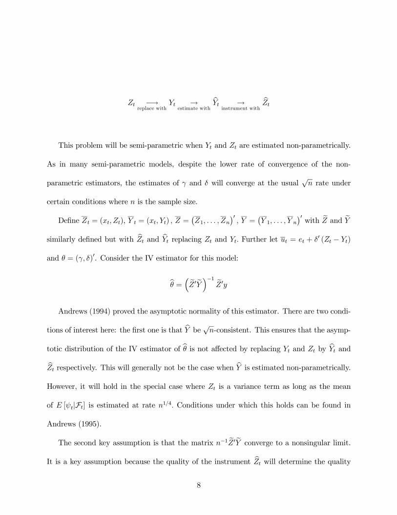
Zt −→replace with
Yt →estimate with
bYt →instrument with
bZt
This problem will be semi-parametric when Yt and Zt are estimated non-parametrically.
As in many semi-parametric models, despite the lower rate of convergence of the non-
parametric estimators, the estimates of γ and δ will converge at the usual√n rate under
certain conditions where n is the sample size.
Define Zt = (xt, Zt), Y t = (xt, Yt) , Z =¡Z1, . . . , Zn
¢0, Y =
¡Y 1, . . . , Y n
¢0with eZ and eY
similarly defined but with bZt and bYt replacing Zt and Yt. Further let ut = et + δ0 (Zt − Yt)
and θ = (γ, δ)0. Consider the IV estimator for this model:
bθ = ³ eZ 0eY ´−1 eZ 0yAndrews (1994) proved the asymptotic normality of this estimator. There are two condi-
tions of interest here: the first one is that bY be √n-consistent. This ensures that the asymp-totic distribution of the IV estimator of bθ is not affected by replacing Yt and Zt by bYt andbZt respectively. This will generally not be the case when bY is estimated non-parametrically.However, it will hold in the special case where Zt is a variance term as long as the mean
of E [ψt|Ft] is estimated at rate n1/4. Conditions under which this holds can be found in
Andrews (1995).
The second key assumption is that the matrix n−1 eZ 0eY converge to a nonsingular limit.
It is a key assumption because the quality of the instrument bZt will determine the quality8
of the asymptotic approximation obtained by Andrews (1994) . This assumption is nearly
violated in many practical situations, and this is the motivation for the development of the
weak instrument literature. The next section will document this phenomenon for financial
data.
3. Evidence of weak instruments
In the case of interest in which Yt = e2t and Zt = σ2t , it will generally be the case that the
correlation between the two estimates, be2t and bσ2t , is very low, suggesting a weak instrumentproblem. Table 1 shows the value of R2 for the regression of be2t on a constant and bσ2t forthree financial data sets using two different non-parametric estimators.
The first data set analyzed represents monthly excess returns on the Standard and Poor’s
500 between January 1965 and December 1997 measured at the end of each month. The
data is taken from CRSP, and the risk-free rate is the return on three-month Treasury bills.
The second data set is made of monthly returns on the yen-dollar spot rate obtained from
International Financial Statistics between September 1978 and June 1998. Finally, the last
data series consists of quarterly excess holding yields on 6-month versus 3-month Treasury
bills between 1959:1 and 2000:2. A similar, but shorter, data set has already been analyzed
by Engle, Lilien, and Robins (1987) using their ARCH-M methodology and Pagan and Hong
(1991) using the above instrumental variable estimator. The three data sets are plotted in
figure 1.
**** Insert figure 1 here ****
9
The first nonparametric estimator is based on multivariate leave-one out kernel. First,
we estimate the mean of yt and y2t ,denoted τ 1t and τ 2t respectively, as:
bτ jt =P
i 6=t yjiK³wi−wtbj
´P
i6=tK³wi−wtbj
´for j = 1, 2 with the kernel function K (w) taken to be the multivariate standard normal.
The bandwidth bj and the number of lags of yt in the conditioning set pj are selected using a
modified version of the criterion suggested in Tjostheim and Auestad (1994) that penalizes
small bandwidths and large lag lengths. Accordingly, we choose the bandwidth (bj) and lag
length (pj) so as to minimize
ln
"1
n
nXt=1
¡yjt − bτ jt¢2
#+lnn
n
µK (0)
bj
¶pj Pnt=1
(yjt−bτjt)2f(wt)Pn
t=1
¡yjt − bτ jt¢2
whereK (0) is the kernel evaluated at 0 and f (wt) is the density of the conditioning variables.
The bandwidth takes the form:
bj = cjsn− 14+pj
where s is the standard deviation of yt and cj is a constant to be selected. We then define
be2t = (yt − bτ 1t)2 and obtain an estimate of σ2t as:bσ2t = bτ 2t − (bτ 1t)2 .
A theoretical analysis of this non-parametric estimator of the conditional variance can
be found in Masry and Tjostheim (1995). In order to avoid unbelievably small bandwidth
choices for all three series, we left out outliers in the bandwidth selection process. The
extreme 25% of the data was not used in the computation of the information criteria.
10
The second estimator was first proposed by Engle and Ng (1993). It provides more
structure to the conditional variance and will approximate the conditional variance function
much better than the kernel when the variance is persistent (see Perron (1999) for simulation
evidence). The estimator is implemented by first estimating the mean by a kernel estimate
as above and then fitting an additive function for σ2t as follows:
σ2t = ω + f1 (bet−1) + . . .+ fp (bet−p) + βσ2t−1
where the fj (·) are estimated as splines with knots using a Gaussian likelihood function. This
allows for a flexible effect of recent information on the conditional variance while allowing for
persistence. This framework includes most parametric models suggested in the literature such
as the GARCH class. The number of segments in the spline functions acts as a smoothing
parameter and is selected using BIC. The knots in the spline were selected using the order
statistics such that each bin has roughly the same number of observation subject to the
constraint of an equal number of bins in the positive and negative regions.
**** Insert table 1 here ****
A quick look at table 1 reveals that only the excess holding yield data has R2 greater
than 5.5%. The reason for this low correlation is that e2t and σ2t have very different volatility.
Even if E [e2t |Ft] = σ2t , financial returns are extremely volatile and therefore, the difference
between e2t and σ2t can be quite large. This is true even if we did not have to estimate these
two quantities; having to estimate them complicates matters further. We can illustrate by
11
looking at the GARCH(1,1) model:
yt = µ+ σtεt = µ+ et
σ2t = ω + αe2t−1 + βσ2t−1.
Andersen and Bollerslev (1998) show that the population R2 in the regression
(yt − µ)2 = a0 + a1bσ2t + vtwhere bσ2t is the one-period ahead forecast obtained from the GARCH model is
R2 =α2
1− β2 − 2αβ
which will in general be very small even though E£(yt − µ)2 |Ft
¤= σ2t . Figure 2 plots the
value of R2 for different values of α and β for thsi GARCH(1,1) example. The value of
R2 is highly sensitive to the value of α, and this reflects that α = 0 makes the model
unidentified. It is usual in the literature to find point estimates of GARCH(1,1) models in
the neighborhood of α = 0.05 and β = 0.9. The figure clearly shows that for such values,
the correlation between e2t and σ2t will typically be quite low. The problem in this case is
that σ2t has very low variance relative to that of y2t ; a low value of α means that σ
2t is nearly
constant locally.
**** Insert figure 2 here ****
We can expect that table 1 does not even provide an accurate picture of the problem of
weak instruments. Using data sampled at higher frequency (e.g. daily or even intra-day)
12
would result in even lower correlation. The lower frequency allows some averaging which
reduces the variance of e2t . Potentially a better solution is to use “model-free” measures of
volatility such as those proposed by Andersen, Bollerslev, Diebold, and Labys (2001) which
are obtained by summing squared returns from higher frequency data. We do not pursue
this possibility here, but note that its variance-reducing property could be helpful in this
context.
4. Asymptotics with weak instruments
Staiger and Stock (1997) have recently shown, in the framework of a linear simultaneous
equation system, that having instruments that are weakly correlated with the explanatory
variables makes the usual asymptotic theory work poorly. Their assumed model is:
y = Y δ +Xγ + u (4.1)
Y = ZΠ+XΓ+ V (4.2)
where Y is the matrix of included endogenous variables that are to be replaced by at least
k2 instruments. Since in our case, it will always be true that the model is exactly identified
(that is, there will be as many regressors as instruments since the instruments are estimates
of the expected value of the regressors), we will concentrate on the case where Z is a n× k2
matrix. The weak instrument assumption is imposed by assuming that:
Π =G√n
(4.3)
13
for some fixed k2 × k2 matrix G 6= 0 This assumption implies that in the limit, Y and Z are
uncorrelated.
We extend the analysis of weak instruments in Staiger and Stock (1997) to our case of
interest by allowing Y and Z to be unobserved and estimated by bY and bZ respectively.
Moreover, we allow for the possibility of higher-order dependence between the instruments
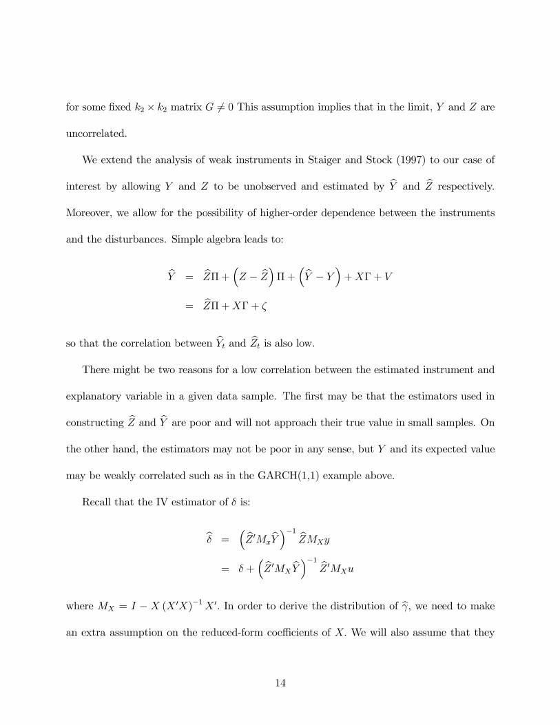
and the disturbances. Simple algebra leads to:
bY = bZΠ+ ³Z − bZ´Π+ ³bY − Y ´+XΓ+ V
= bZΠ+XΓ+ ζ
so that the correlation between bYt and bZt is also low.There might be two reasons for a low correlation between the estimated instrument and
explanatory variable in a given data sample. The first may be that the estimators used in
constructing bZ and bY are poor and will not approach their true value in small samples. Onthe other hand, the estimators may not be poor in any sense, but Y and its expected value
may be weakly correlated such as in the GARCH(1,1) example above.
Recall that the IV estimator of δ is:
bδ =³ bZ 0Mx
bY ´−1 bZMXy
= δ +³ bZ 0MX
bY ´−1 bZ 0MXu
where MX = I − X (X 0X)−1X 0. In order to derive the distribution of bγ, we need to makean extra assumption on the reduced-form coefficients of X. We will also assume that they
14
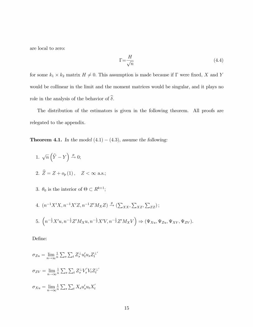
are local to zero:
Γ=H√n
(4.4)
for some k1 × k2 matrix H 6= 0. This assumption is made because if Γ were fixed, X and Y
would be collinear in the limit and the moment matrices would be singular, and it plays no
role in the analysis of the behavior of bδ.The distribution of the estimators is given in the following theorem. All proofs are
relegated to the appendix.
Theorem 4.1. In the model (4.1)− (4.3), assume the following:
1.√n³bY − Y ´ p→ 0;
2. bZ = Z + op (1) , Z <∞ a.s.;
3. θ0 is the interior of Θ ⊂ Rk+1;
4. (n−1X 0X, n−1X 0Z, n−1Z 0MXZ)p→ (P
XX ,P
XZ,P
ZZ) ;
5.³n−
12X 0u, n−
12Z 0MXu, n
− 12X 0V, n−
12Z 0MXV
´⇒ (ΨXu,ΨZu,ΨXV ,ΨZV ).
Define:
σZu = limn→∞
1n
Ps
Pt Z
⊥s u
0tusZ
⊥0t
σZV = limn→∞
1n
Ps
Pt Z
⊥s V
0sVtZ
⊥0t
σXu = limn→∞
1n
Ps
PtXsu
0sutX
0t
15
σXV = limn→∞
1n
Ps
PtXsV
0sVtX
0t
ρZ = limn→∞
1n
Pnt=1
Pns=1 Z
⊥t V
0t σ−120
ZV σ− 12
ZuusZ⊥0s
ρX = limn→∞
1n
Pnt=1
Pns=1XtV
0t σ− 120
Zv σ− 12
ZuusXs
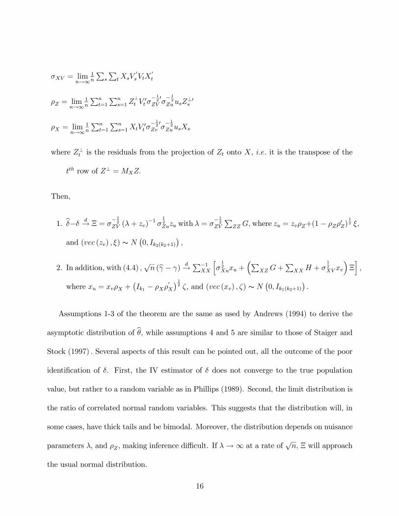
where Z⊥t is the residuals from the projection of Zt onto X, i.e. it is the transpose of the
tth row of Z⊥ =MXZ.
Then,
1. bδ−δ d→ Ξ = σ− 12
ZV (λ + zv)−1 σ
12Zuzu with λ = σ
−12
ZV
PZZ G,where zu = zvρZ+(1− ρZρ
0Z)
12 ξ,
and (vec (zv) , ξ) ∼ N¡0, Ik2(k2+1)
¢,
2. In addition, with (4.4) ,√n (bγ − γ)
d→P−1XX
hσ12Xuxu +
³PXZ G+
PXX H + σ
12XV xv
´Ξi,
where xu = xvρX +¡Ik1 − ρXρ
0X
¢ 12 ζ, and (vec (xv) , ζ) ∼ N
¡0, Ik1(k2+1)
¢.
Assumptions 1-3 of the theorem are the same as used by Andrews (1994) to derive the
asymptotic distribution of bθ, while assumptions 4 and 5 are similar to those of Staiger andStock (1997) . Several aspects of this result can be pointed out, all the outcome of the poor
identification of δ. First, the IV estimator of δ does not converge to the true population
value, but rather to a random variable as in Phillips (1989). Second, the limit distribution is
the ratio of correlated normal random variables. This suggests that the distribution will, in
some cases, have thick tails and be bimodal. Moreover, the distribution depends on nuisance
parameters λ, and ρZ , making inference difficult. If λ→∞ at a rate of√n, Ξ will approach
the usual normal distribution.
16
In addition, the distribution of the coefficients on the exogenous variables xt is conta-
minated by the poor identification of δ. Specifically, we expect that the usual standard
errors will understate the true uncertainty as these are based on the first term of the limiting
distribution only. This will lead to over-rejection of hypotheses of the type H0 : γ = γ0.
The basic distribution theory described above is very closely related to that derived by
Staiger and Stock. The form of the covariance matrix is different because we do not assume
that the instruments, Zt, are independent of the error terms ut and vt; we only assume
that they are uncorrelated. This adjustment allows for higher-order dependence between Zt
on the one hand and ut and vt on the other. In cases where there is no higher dependence
between the instruments and the error terms, this distribution coincides with the one derived
by Staiger and Stock.
The assumptions on the properties of the data are given in terms of high-level conditions, a
joint weak law of large numbers and a weak convergence result. This is done to make the con-
ditions similar to those used by Staiger and Stock. Many sets of primitive conditions can lead
to these two results. For example, sufficient conditions are that the vector (ut, Vt) be a mar-
tingale difference sequence with respect to the filtration©(ut−j−1, Vt−j−1, Zt−j ,Xt−j) , j ≥ 0
ªwith uniform finite (2 + η) moments for some η > 0 and the vector (Zt, Xt) be α-mixing
with mixing numbers of size −κ/ (κ− 1) and (r + κ) finite moments for some r ≥ 2. These
conditions imply that in the variance case, Zt = σ2t , we need σ8t to be finite for all t. This is
a difficult requirement for financial data as there is some evidence that many financial series
do not even have four finite moments. For this reason, we will use highly aggregated data
17
(for example monthly and quarterly data) for applications. However, our simulation results
will show that reliable inference can still be done even under moment condition failure.
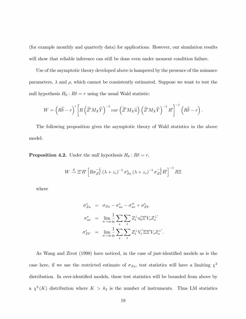
Use of the asymptotic theory developed above is hampered by the presence of the nuisance
parameters, λ and ρ, which cannot be consistently estimated. Suppose we want to test the
null hypothesis H0 : Rδ = r using the usual Wald statistic:
W =³Rbδ − r´0 ·R³ bZ 0MX
bY ´−1 var ³ bZ 0MXbu´³ bZ 0MXbY ´−1R0¸−1 ³Rbδ − r´ .
The following proposition gives the asymptotic theory of Wald statistics in the above
model:
Proposition 4.2. Under the null hypothesis H0 : Rδ = r,
Wd→ Ξ0R0
hRσ
− 12
ZV (λ+ zv)−1 σ∗Zu (λ+ zv)
−1 σ− 12
ZVR0i−1
RΞ
where
σ∗Zu = σZu − σ∗uv − σ∗0uv + σ∗ZV
σ∗uv = limn→∞
1
n
Xs
Xt
Z⊥t u0tΞ0VsZ⊥
0s
σ∗ZV = limn→∞
1
n
Xs
Xt
Z⊥t V0t ΞΞ
0VsZ⊥0
s .
As Wang and Zivot (1998) have noticed, in the case of just-identified models as is the
case here, if we use the restricted estimate of σZu, test statistics will have a limiting χ2
distribution. In over-identified models, these test statistics will be bounded from above by
a χ2 (K) distribution where K > k2 is the number of instruments. Thus LM statistics
18
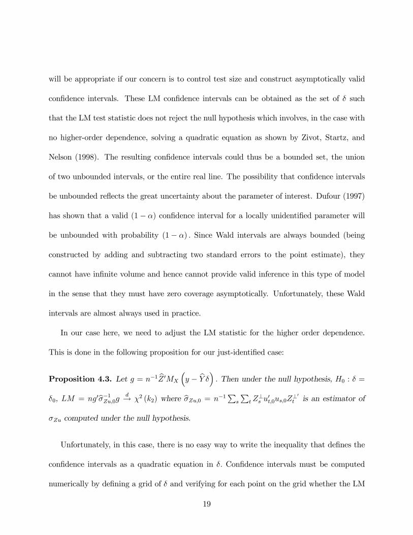
will be appropriate if our concern is to control test size and construct asymptotically valid
confidence intervals. These LM confidence intervals can be obtained as the set of δ such
that the LM test statistic does not reject the null hypothesis which involves, in the case with
no higher-order dependence, solving a quadratic equation as shown by Zivot, Startz, and
Nelson (1998). The resulting confidence intervals could thus be a bounded set, the union
of two unbounded intervals, or the entire real line. The possibility that confidence intervals
be unbounded reflects the great uncertainty about the parameter of interest. Dufour (1997)
has shown that a valid (1− α) confidence interval for a locally unidentified parameter will
be unbounded with probability (1− α) . Since Wald intervals are always bounded (being
constructed by adding and subtracting two standard errors to the point estimate), they
cannot have infinite volume and hence cannot provide valid inference in this type of model
in the sense that they must have zero coverage asymptotically. Unfortunately, these Wald
intervals are almost always used in practice.
In our case here, we need to adjust the LM statistic for the higher order dependence.
This is done in the following proposition for our just-identified case:
Proposition 4.3. Let g = n−1 bZ 0MX
³y − bY δ´ . Then under the null hypothesis, H0 : δ =
δ0, LM = ng0bσ−1Zu,0g d→ χ2 (k2) where bσZu,0 = n−1P
s
Pt Z
⊥s u
0t,0us,0Z
⊥0t is an estimator of
σZu computed under the null hypothesis.
Unfortunately, in this case, there is no easy way to write the inequality that defines the
confidence intervals as a quadratic equation in δ. Confidence intervals must be computed
numerically by defining a grid of δ and verifying for each point on the grid whether the LM
19
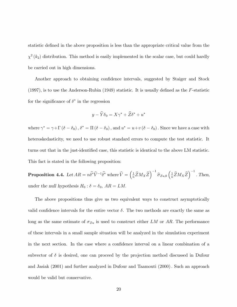
statistic defined in the above proposition is less than the appropriate critical value from the
χ2 (k2) distribution. This method is easily implemented in the scalar case, but could hardly
be carried out in high dimensions.
Another approach to obtaining confidence intervals, suggested by Staiger and Stock
(1997), is to use the Anderson-Rubin (1949) statistic. It is usually defined as the F -statistic
for the significance of δ∗ in the regression
y − bY δ0 = Xγ∗ + bZδ∗ + u∗where γ∗ = γ+Γ (δ − δ0) , δ
∗ = Π (δ − δ0) , and u∗ = u+v (δ − δ0) . Since we have a case with
heteroskedasticity, we need to use robust standard errors to compute the test statistic. It
turns out that in the just-identified case, this statistic is identical to the above LM statistic.
This fact is stated in the following proposition:
Proposition 4.4. LetAR = nbδ∗bV −1 bδ∗ where bV = ³ 1nbZMX
bZ´−1 bσZu,0 ³ 1n bZMXbZ´−1 .Then,
under the null hypothesis H0 : δ = δ0, AR = LM.
The above propositions thus give us two equivalent ways to construct asymptotically
valid confidence intervals for the entire vector δ. The two methods are exactly the same as
long as the same estimate of σZu is used to construct either LM or AR. The performance
of these intervals in a small sample situation will be analyzed in the simulation experiment
in the next section. In the case where a confidence interval on a linear combination of a
subvector of δ is desired, one can proceed by the projection method discussed in Dufour
and Jasiak (2001) and further analyzed in Dufour and Taamouti (2000) . Such an approach
would be valid but conservative.
20
In a related paper, Dufour and Jasiak (2001) have obtained exact tests based on AR-type
statistics in models with generated regressors and weak instruments. However, their results
only apply to parametrically-estimated regressors that will converge at rate√n and not to
the non-parametric estimators analyzed here.
Startz, Nelson, and Zivot (2001) have developed an alternative set of statistics, which
they call S statistics, that take into account the degree of identification. They show in the
case of a single regressor and instrument (k1 = k2 = 1) that these are equivalent to the AR
statistic. We suspect that this correspondence is more general and carries over to the exactly
identified case that we treat here, but we have no proof for this conjecture.
5. Simulation Results
In this section, the behavior of the procedures described above will be analyzed through a
small simulation experiment. Important issues to be analyzed include the choice of smoothing
parameters, the appropriateness of the various confidence intervals, and the distribution of
the resulting estimators.
Consider the GARCH-M(1, 1) DGP:
yt = γ + δσ2t + et = γ + δσ2t + σtεt
σ2t = ω + αe2t−1 + βσ2t−1
εt ∼ i.i.d. (0, 1)
In terms of the above notation, we have vt = e2t − σ2t , ut = et − δvt, Yt = e2t , and Zt = σ2t .
21

The distribution of εt is either normal or Student t. This allows us to check the robustness
of the procedures to the restrictive moment assumptions required by the asymptotic theory
developed above. We use six sets of parameters, all estimated from data, which are presented
in table 2.
**** Insert table 2 here ****
The point estimates for the stock data are similar to those usually obtained in this
context, for example by Glosten, Jagannathan, and Runkle (1993), and will lead to a rather
persistent σ2t and to a weak instrument. Sample sizes of 450, 300, and 150 are used for
the experiments, with the first 50 observations deleted to remove the effect of the initial
condition (taken as the mean of the unconditional distribution). The length of the samples
nearly match those of the S&P, exchange rate, and excess holding yield data.
One disadvantage of the current setup is that the correlation between bσ2t and be2t cannotbe controlled. We can control the correlation between the unobservable variables, but due
to estimation, the correlation between observable variables will be different in general.
The values of the nuisance parameters in this setup can be obtained in terms of the
22
moments of the conditional variance process as:
σZV = (κ4 − 1)hE¡σ8t¢− 2E ¡σ2t ¢E ¡σ6t ¢+ E ¡σ2t¢2E ¡σ4t¢i
σZu = δ2σZv + E¡σ6t¢− 2E ¡σ2t¢E ¡σ4t¢+ E ¡σ2t ¢3
−2δκ3hE¡σ7t¢− 2E ¡σ5t ¢E ¡σ2t ¢+ E ¡σ3t¢E ¡σ2t¢2i
ρZ =−δσZv + κ3
hE (σ7t )− 2E (σ5t )E (σ2t ) + E (σ3t )E (σ2t )2
iσ12Zuσ
12ZV
λ =
√nhE (σ4t )− E (σ2t )2
iσ12Zv
σ∗Zu = σZu − 2σuvΞ+ σZV Ξ2
where κj = E¡εjt¢is the jth moment of εt. The values of the first 4 even moments of σ2t are
derived recursively in Bollerslev (1986) as a function of ω, α, and β and the moments of εt.
This allows for the easy computation of the nuisance parameters which are included in table
2. Note that the moment condition assumed in theorem 4.1 is only satisfied for the first two
sets of parameters.
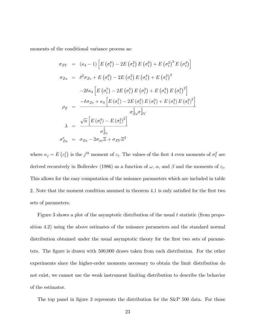
Figure 3 shows a plot of the asymptotic distribution of the usual t statistic (from propo-
sition 4.2) using the above estimates of the nuisance parameters and the standard normal
distribution obtained under the usual asymptotic theory for the first two sets of parame-
ters. The figure is drawn with 500,000 draws taken from each distribution. For the other
experiments since the higher-order moments necessary to obtain the limit distribution do
not exist, we cannot use the weak instrument limiting distribution to describe the behavior
of the estimator.
The top panel in figure 3 represents the distribution for the S&P 500 data. For those
23
values of the parameters, the t statistic has a highly skewed distribution. On the other hand,
the bottom panel reveals that for the second experiment, the t statistic is both highly skewed
and has fat tails. In fact, a good part of the probability mass (about 7 %) lies outside of
the [−4, 4] interval. The shape of the distribution is controlled by 2 nuisance parameters, λ
and ρZ . These experiments show that low λ and high |ρZ | give distributions very far from
normality. To measure the impact of these properties on coverage probabilities, note that
only 77.7% of the mass is between -1.96 and 1.96 in the bottom panel, while the same figure is
96.5% in the top panel. We conclude that the first experiment will have usual (Wald-based)
95% confidence intervals with coverage rates higher than their nominal level, while those in
the second experiment will exhibit low coverage.
**** Insert figure 3 here ****
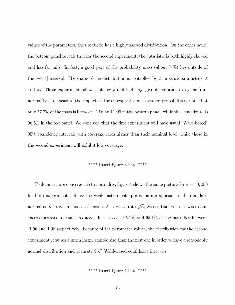
To demonstrate convergence to normality, figure 4 shows the same picture for n = 50, 000
for both experiments. Since the weak instrument approximation approaches the standard
normal as n → ∞ in this case because λ → ∞ at rate√n, we see that both skewness and
excess kurtosis are much reduced. In this case, 95.2% and 95.1% of the mass lies between
-1.96 and 1.96 respectively. Because of the parameter values, the distribution for the second
experiment requires a much larger sample size than the first one in order to have a reasonably
normal distribution and accurate 95% Wald-based confidence intervals.
**** Insert figure 4 here ****
24
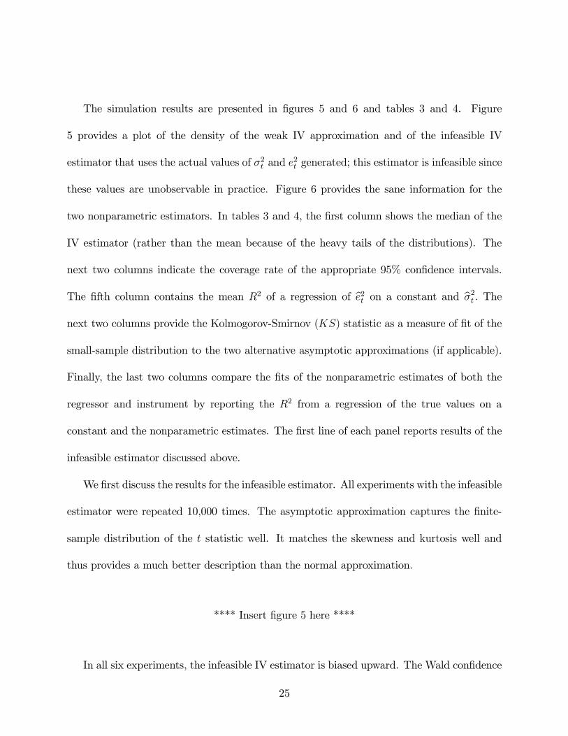
The simulation results are presented in figures 5 and 6 and tables 3 and 4. Figure
5 provides a plot of the density of the weak IV approximation and of the infeasible IV
estimator that uses the actual values of σ2t and e2t generated; this estimator is infeasible since
these values are unobservable in practice. Figure 6 provides the sane information for the
two nonparametric estimators. In tables 3 and 4, the first column shows the median of the
IV estimator (rather than the mean because of the heavy tails of the distributions). The
next two columns indicate the coverage rate of the appropriate 95% confidence intervals.
The fifth column contains the mean R2 of a regression of be2t on a constant and bσ2t . Thenext two columns provide the Kolmogorov-Smirnov (KS) statistic as a measure of fit of the
small-sample distribution to the two alternative asymptotic approximations (if applicable).
Finally, the last two columns compare the fits of the nonparametric estimates of both the
regressor and instrument by reporting the R2 from a regression of the true values on a
constant and the nonparametric estimates. The first line of each panel reports results of the
infeasible estimator discussed above.
We first discuss the results for the infeasible estimator. All experiments with the infeasible
estimator were repeated 10,000 times. The asymptotic approximation captures the finite-
sample distribution of the t statistic well. It matches the skewness and kurtosis well and
thus provides a much better description than the normal approximation.
**** Insert figure 5 here ****
In all six experiments, the infeasible IV estimator is biased upward. The Wald confidence
25

intervals have a coverage rate that is higher than its nominal level for the S&P data and
lower (and sometimes much lower) for the other two data sets, while the LM interval has
coverage rate that is only slightly too low in all cases. Not surprisingly, the weak instrument
approximation is more accurate according to the KS statistic in both cases where it can
be computed. The improvement is much more dramatic in the very non-normal case of
experiment 2. Note also that the overall results are not sensitive to conditional normality or
the existence of moments.
**** Insert tables 3 and 4 here ****
We now turn our attention to the semi-parametric estimators. Estimates of e2t and σ2t are
obtained using the same two nonparametric methods as above, either a kernel or the semi-
parametric Engle-Ng estimator using data-based selection for all smoothing parameters.
Each experiment with the non-parametric estimators was repeated 5000 times.
The need to estimate σ2t and e2t changes the result quite dramatically relative to the
infeasible estimator. The results using the kernel estimates are presented in the second row
of each panel of tables 3 and 4 and as the dashed line in figure 6, while those for the Engle-Ng
are presented in the third row of each panel and as the dotted line in figure 6. Overall, the
Engle-Ng procedure leads to an IV estimator that much more closely matches the infeasible
one. In particular, its distribution has a similar shape to that of the infeasible IV (and
that of the weak IV approximation), and the coverage rate of the confidence intervals based
on it are much closer to those of the infeasible estimator. The reason for this is clear: it
26
provides a better approximation to the instrument (σ2t ) than does the kernel as evidence by
the higher R2 in the regression of true conditional variance on a constant and its estimate
which is consistent with the simulation evidence in Perron (1999) .The regressor (e2t ) is well
approximated by any method. Note also that once we estimate the regressor and instrument,
the IV estimator of δ is strongly biased towards zero (with the exception of experiment 3).
**** Insert figure 6 here ****
An important practical result is that LM-based confidence intervals are more robust
(in terms of having correct coverage) to both the presence of weak instruments and to
the estimation of regressors and instruments. In all cases, the coverage rate of LM-based
confidence intervals is closer to 95% than Wald—based intervals. If, in addition, the Engle-Ng
estimator is used, coverage is almost exact. These should therefore be preferred in empirical
work.
Table 5 provides details on the nonparametric estimators used in the simulation. We
report the mean bandwidth constant, lag length selected, sum of the first 10 squared auto-
correlation coefficients of the variance residuals, as well as the median constant and slope
coefficient from the regression of the true instrument and regressor on a constant and the
non-parametric estimates. The R2 from these regressions has already been reported in tables
3 and 4.
**** Insert table 5 here ****
27

The BIC-type criterion seems to overpenalize the number of lags as it always chooses a
single lag for all kernel estimates. However, it does suggest that some oversmoothing relative
to the i.i.d. normal case is typically warranted (since in that case, the optimal bandwidth
constant is 1.06). This is not surprising and is usually the case for dependent data. The
criterion also seems to penalize heavily the number of bins in the Engle-Ng estimator as the
mean number of bins is not much above 2. However, it frequently chooses more than one
lag.
The main feature of table 5 however is the tight relation between the bias of the in-
strument estimates and the behavior of the resulting IV estimator relative to the infeasible
estimator. In cases where the IV estimator with estimated regressor and instrument per-
forms poorly (experiments 2, 5, and 6 for both estimators and experiment 4 for the kernel
only), the median slope parameter from the instrument regression is always less than 0.5,
suggesting a severe bias of the nonparametric estimator. This result is akin to the typical
result in semiparametric estimation that it is preferable to undersmooth the nonparamet-
ric component so as to reduce bias. The averaging in the second step mitigates the higher
variance that this undersmoothing typically entails, while it does not eliminate bias.
6. Empirical results
In this section, we analyze our three financial data sets to seek evidence of a risk-return trade-
off. To reiterate, the series are monthly returns on the S&P 500 index, monthly returns on
the yen-dollar spot rate, and quarterly excess holding yield between 6-month and 3-month
28
Treasury bills. For each series, we postulate a model of the form
yt = γ + δσ2t + et
with σ2t = E£yt − E [yt|Ft−1]2 |Ft−1¤ where Ft−1 are lagged values of yt. For all three
series, the conditional variance was estimated using either the kernel or Engle-Ng estimator
described above with the data-based selection of the tuning parameters. For comparison,
we also report the results from a GARCH-M(1, 1) model estimated using Gaussian quasi-
maximum likelihood.
The convergence to normality shown in the simulation might suggest that the use of higher
frequency data is greatly desirable as it would increase sample size, but higher frequency
would also lead to a more persistent conditional variance and hence a weaker instrument.
The impact of this choice on the behavior of the IV estimator and its related statistics is
therefore ambiguous. As discussed already, another potential use of high-frequency data (not
pursued here) is to get better estimates of low-frequency volatility.
The estimation results are presented in table 6. In addition to the point estimates and
their robust (White) standard errors, we present Wald-based and LM-based 95% confidence
intervals for the coefficient on the risk variable, δ, the R2 in a regression of bσ2t on be2t anda constant, and the values of the tuning parameters used to construct the nonparametric
estimates. The LM confidence intervals were computed by numerically inverting the LM
statistic using a grid of 20,000 equi-spaced points between -1000 and 1000. For this reason,
the infinite or very large confidence intervals are truncated at these two endpoints.
The trade-off between risk and return has been extensively studied for stocks with con-
29

flicting results. For example, French, Schwert, and Stambaugh (1987) find a positive rela-
tion between returns and the conditional variance, while Glosten, Jagannathan, and Runkle
(1993) find a negative relationship using a modified GARCH-M methodology. This conflict-
ing evidence is not surprising in light of the results obtained by Backus, Gregory, and Zin
(1989) and Backus and Gregory (1993). Using a general equilibrium setting, they provide
simulation evidence that the relationship between expected returns and the variance of re-
turns can go in either direction, depending on specification. Further doubt on the validity
of the linearity assumption is provided in Linton and Perron (2000) using non-parametric
methods.
Our results suggest that no significant risk premium exists in stock returns using any of
the three methods. However, the main feature of the results is the wider confidence intervals
obtained using the LM principle. Wald confidence intervals understate the uncertainty of
the estimated parameters; the differences are not dramatic however. The results are also
similar to those obtained from the GARCH-M(1,1) model.
**** Insert table 6 here ****
The results for the yen-dollar returns are presented next with all point estimates negative.
In the case of the kernel estimator, this finding is actually significantly different from 0. The
relationship for this series appears to be the least identified as all estimators have large
standard errors (and the first-stage R2 is very low). Both the Wald and LM confidence
intervals are quite wide, reflecting poor identification of the model. The LM interval with
30

the Engle-Ng estimator is even unbounded in this case.
Finally, the results of the estimation for excess holding yields present a similar picture.
All point estimates are positive, with the GARCH-M result being significantly different from
0. This conclusion is the same as Engle, Lillien, and Robbins (who used a restricted ARCH-
M(4) structure). For the kernel estimator, the effect is almost significant at the 5% level.
Once again, the LM intervals are much wider than their Wald counterparts.
Figure 7 presents a time plot of the estimated conditional variance for all three series.
Except for the excess holding yield, the Engle-Ng and GARCH-M models offer a very similar
picture. On the other hand, the kernel estimates are much more volatile (not surprisingly
given than they do not have an autoregressive structure) over time. The results for the
excess holding yield might seem strange at first sight since the GARCH-M gives such a
different picture (especially around the Volker experiment of 1979-82). The reason lies in
the bandwidth choice for the estimation of the conditional mean of this series. The mean is
estimated with a very small bandwidth (constant is 0.28) thus implying little smoothing of
neighboring observations, and as a result, the residuals are much smaller than with GARCH-
M (and hence have smaller variance).
**** Insert figure 7 here ****
31
7. Conclusion
This paper follows several others in showing that inference using instrumental variables is
greatly affected by a low correlation between the instruments and the explanatory variables.
It extends the current literature to linear semi-parametric models with non-parametrically es-
timated regressors and instruments and to cases with higher-order dependence. The analysis
shows that the limit theory is similar to that currently available in the literature.
Simulation evidence reveals that the additional step of estimating both the regressors
and the instruments may lead to a loss in the quality of asymptotic approximations. Using a
semi-parametric estimator proposed by Engle and Ng (1993) and carrying out inference using
Lagrange Multiplier procedures allows for inference that is more robust than the alternatives
considered here.
Empirical application to three financial series suggests that conclusions may hinge on
the use of appropriate confidence intervals. Using the appropriate LM confidence intervals
and the semi-parametric estimator of the conditional variance leads us to conclude that
none of the series considered includes a statistically significant risk premium. This differs in
some cases from inference based on the usual Wald confidence intervals and on a parametric
GARCH-M model. However, because of the wide confidence intervals, the results are also
consistent with the presence of large risk premia. The data is simply not informative enough
to precisely estimate the relationship between risk and returns.
Further work on this problem is clearly warranted. In particular, other more commonly
used estimators such as maximum likelihood are likely to face similar problems as the IV
32

estimator analyzed here. This analysis could follow the methodology developed in Stock
and Wright (2000) for GMM estimators. Finally, a critical avenue for future research is
the development of techniques to diagnose cases where weak identification hinders inference
using usual methods. Recent testing procedures along these lines have been suggested by
Arellano, Hansen, and Sentana (1999) ,Wright (2000) , and Hahn and Hausman (2002) .
33

REFERENCES
Andersen, Torben G. and Tim Bollerslev, “Answering the Critics: Yes, ARCH Models
Do Provide Good Volatility Forecasts”, International Economic Review, 39, November
1998, 885-905.
Andersen, Torben G., Tim Bollerslev, Francis X. Diebold, and Paul Labys, “The Dis-
tribution of Realized Exchange Rate Volatility”, Journal of the American Statistical
Association, 96, March 2001, 42-55.
Anderson, T. W. and Herman Rubin, “Estimation of the Parameters of a Single Equation
in a Complete System of Stochastic Equations”, Annals of Mathematical Statistics, 20,
March 1949, 46-63.
Andrews, Donald W. K., “Asymptotics for Semiparametric Econometric Models via Sto-
chastic Equicontinuity”, Econometrica, 62, January 1994, 43-72.
Andrews, DonaldW. K., “Examples of MINPIN Estimators: Supplement to Asymptotics for
Semiparametric Models via Stochastic Equicontinuity”, manuscript, Yale University,
1992.
Andrews, Donald W. K., “Nonparametric Kernel Estimation for Semiparametric Models”,
Econometric Theory, 11, August 1995, 560-596.
Arellano, Manuel, Lars P. Hansen, and Enrique Sentana, “Underidentification?”, manu-
script, CEMFI, July 1999.
34
Backus, David K., Allan W. Gregory, and Stanley E. Zin, “Risk Premiums in the Term
Structure: Evidence from Artificial Economies”, Journal of Monetary Economics, 24,
November 1989, 371-399.
Backus, David K. and Allan W. Gregory , “Theoretical Relations Between Risk Premiums
and Conditional Variances,” Journal of Business and Economic Statistics, 11, April
1993, 177-185.
Bollerslev, Tim, “Generalized Conditional Heteroskedasticity”, Journal of Econometrics,
31, April 1986, 307-327.
Bottazzi, Laura and Valentina Corradi, “Analysing the Risk Premium in the Italian Stock
Market: ARCH-M Models versus Non-parametric Models”, Applied Economics, 23,
March 1991, 535-542.
Braun, Phillip A., Daniel B. Nelson, and Alain M. Sunier, “Good News, Bad News, Volatil-
ity and Betas”, Journal of Finance, 50, december 1995, 1575-1604.
Chao, John. and Norman. R. Swanson, “Bias and MSE of the IV Estimator Under Weak
Identification”, manuscript, University of Maryland and Purdue University, August
2001.
Choi, In and Peter C. B. Phillips, “Asymptotic and Finite Sample Distribution Theory for
the IV Estimators and Tests in Partially Identified Structural Relations”, Journal of
Econometrics, 51, February 1992, 113-150.
35
Dufour, Jean-Marie, “Some Impossibility Theorems in Econometrics with Applications to
Instrumental Variables, Dynamic Models, and Cointegration”, Econometrica, 65, No-
vember 1997, 1365-1387.
Dufour, Jean-Marie and Joann Jasiak, “Finite Sample Inference Methods for Simultane-
ous Equations and Models with Unobserved and Generated Regressors”, International
Economic Review, 42, August 2001, 815-843.
Dufour, Jean-Marie and Mohamed Taamouti, “Projection-Based Statistical Inference in
Linear Structural Models with Possibly Weak Instru-ments”, manuscript, Université
de Montréal, 2001.
Engle, Robert F., and Victor K. Ng, “Measuring and Testing the Impact of News on
Volatility”, Journal of Finance, 48, December 1993, 1749-1778.
Engle, Robert F., Lilien, David M., and Russell P. Robins, “Estimating Time Varying Risk
Premia in the Term Structure: The ARCH-M Model”, Econometrica, 55, March 1987,
391-407.
French, Kenneth, G. William Schwert, and Robert F. Stambaugh, “Expected Stock Returns
and Volatility”, Journal of Financial Economics, 19, September 1987, 3-29.
Glosten, Lawrence R., Ravi Jagannathan, and David E. Runkle, “On the Relation Between
the Expected Value and the Volatility of the Nominal Excess Return on Stocks”, Jour-
nal of Finance, 48, December 1993, 1779-1801.
36
Hahn, Jinyong and Jerry Hausman, “A New Specification Test for the Validity of Instru-
mental Variables”, Econometrica, 70, January 2002, 163-189.
Hall, Alastair R., Glenn D. Rudebusch, and David W. Wilcox, “Judging Instrument Rele-
vance in Instrumental Variables Estimation”, International Economic Review, 37, May
1996, 283-298.
Lettau, Martin and Sydney Ludvigson, “Measuring and Modeling Variation in the Risk-
Return Tradeoff”, manuscript, New York University and Federal Reserve Bank of New
York, October 2001.
Linton, Oliver and Benoit Perron, “The Shape of the Risk Premium: Evidence From a
Semiparametric GARCH Model”, CRDE working paper 0899, Université de Montréal,
1999 (revised February 2002).
Masry, Elias and Dag Tjostheim, “Nonparametric Estimation and Identification of Non-
linear Time Series: Strong Convergence and Asymptotic Normality”, Econometric
Theory, 11, June 1995, 258-289.
Nelson, Charles R., Startz, Richard, “The Distribution of the Instrumental Variables Es-
timator and its t-ratio when the Instrument is a Poor One”, Journal of Business, 63,
January 1990, S125-S140.
Pagan, Adrian, “Econometric Issues in the Analysis of Regressions with Generated Regres-
sors”, International Economic Review, 25, February 1984, 221-247.
37
Pagan, Adrian R. and Y. S. Hong, “Nonparametric Estimation and the Risk Premium”
in Barnett, William A., James Powell, and George E. Tauchen eds., Nonparametric
and Semiparametric Methods in Econometrics and Statistics: Proceedings of the Fifth
International Symposium in Economic Theory and Econometrics, Cambridge: Cam-
bridge University Press, 1991, 51-75.
Pagan, Adrian and Aman Ullah. “The Econometric Analysis of Models with Risk Terms”,
Journal of Applied Econometrics, 3, April 1988, 87-105.
Perron, Benoit, “A Monte Carlo Comparison of Non-parametric Estimators of the Condi-
tional Variance”, manuscript, Université de Montréal, 1999.
Phillips, Peter C. B., “Partially Identified Econometric Models”, Econometric Theory, 5,
August 1989, 181-240.
Sentana, Enrique and Sushil Wadhwani, “Semi-parametric Estimation and the Predictabil-
ity of Stock Market Returns: Some Lessons from Japan”, Review of Economics Studies,
58, May 1991, 547-563.
Staiger, Douglas and James H. Stock, “Instrumental Variables Regression with Weak In-
struments”, Econometrica, 65, May 1997, 557-586.
Startz, Richard, Charles R. Nelson, and Eric Zivot, “Improved Inference for the Instrumen-
tal Variable Estimator”, manuscript, Univesity of Washington, February 2001.
Stock, James and Jonathan Wright, “GMM with Weak Identification”, Econometrica, 68,
38
September 2000, 1055-1096.
Tjostheim, Dag and Bjorn H. Auestad, “Nonparametric Identification of Nonlinear Time
Series: Selecting Significant Lags”, Journal of the American Statistical Association, 89,
december 1994, 1410-1419.
Wang, Jiahui and Eric Zivot, “Inference on a Structural Parameter in Instrumental Regres-
sion with Weak Instruments”, Econometrica, 66, November 1998, 1389-1404.
Wright, Jonathan, “Detecting Lack of Identification in GMM”, International Finance Dis-
cussion Paper 674, Board of Governors of the Federal Reserve System, July 2000.
Zivot, Eric, Richard Startz and Charles R. Nelson “Valid Confidence Intervals and Inference
in the Presence of Weak Instruments”, International Economic Review, 39, November
1998, 1119-1144.
39
8. Appendix
A. Proofs
A.1. Preliminary results
Before proving the results in the paper, we will collect the required preliminaries in the
following lemma.
Lemma A.1. Suppose the conditions of theorem (4.1) are satisfied. Then, the following
hold:
1. 1√n
³ bZ 0MXbY ´ = 1√
n(Z 0MXY ) + op (1)
2. 1√n
h bZ 0MX (Z − Y ) δi= 1√
n[Z 0MX (Z − Y ) δ] + op (1)
3. 1√n
³ bZ 0MXe´= 1√
n(Z 0MXe) + op (1)
4. 1n
³ bZ 0MXbZ´ = 1
n(Z 0MXZ) + op (1)
5. 1√nX 0bY = 1√
nX 0Y + op (1)
6. 1√n
h bZ 0MX
³Y − bY ´ δi p→ 0
7. 1√n
³ bZ 0MXu´= ΨZu + op (1) .
40
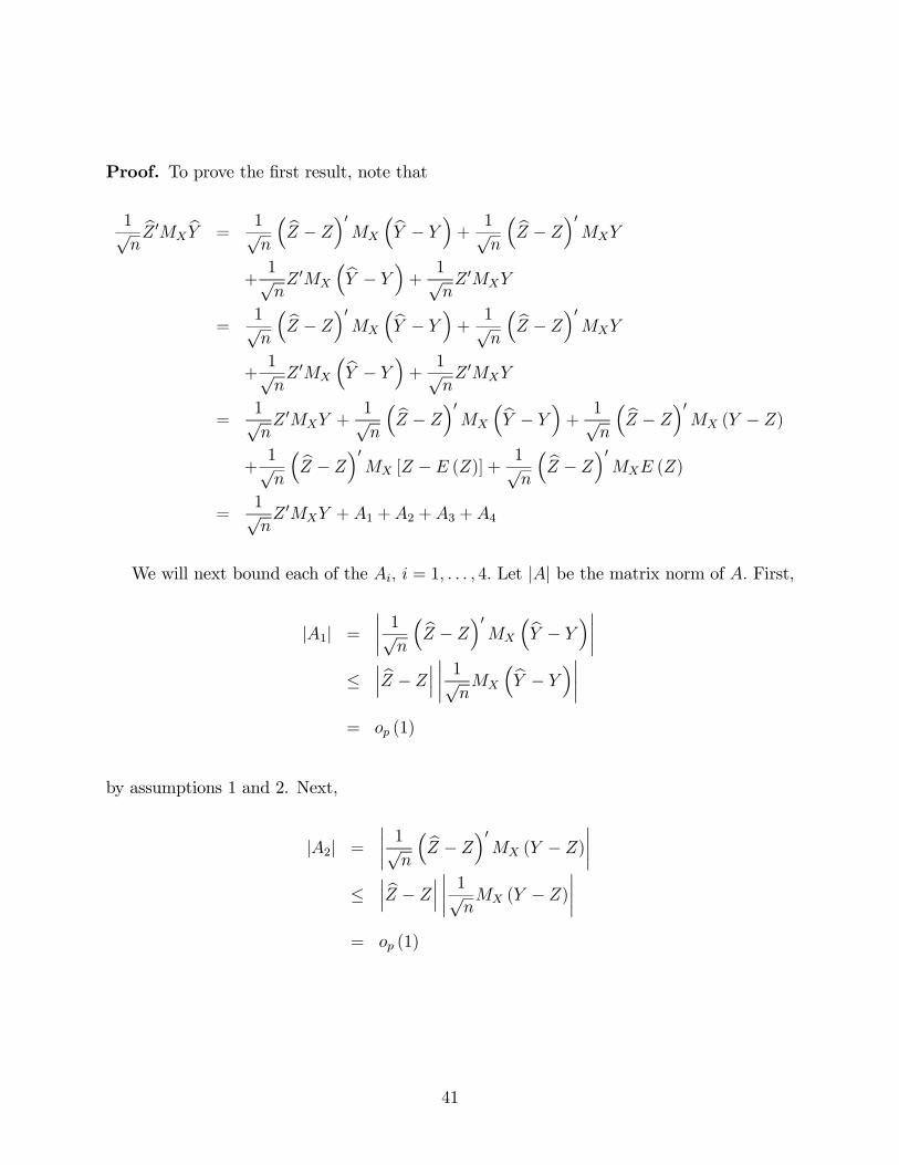
Proof. To prove the first result, note that
1√nbZ 0MX
bY =1√n
³ bZ − Z´0MX
³bY − Y ´+ 1√n
³ bZ − Z´0MXY
+1√nZ 0MX
³bY − Y ´+ 1√nZ 0MXY
=1√n
³ bZ − Z´0MX
³bY − Y ´+ 1√n
³ bZ − Z´0MXY
+1√nZ 0MX
³bY − Y ´+ 1√nZ 0MXY
=1√nZ 0MXY +
1√n
³ bZ − Z´0MX
³bY − Y ´+ 1√n
³ bZ − Z´0MX (Y − Z)
+1√n
³ bZ − Z´0MX [Z − E (Z)] + 1√n
³ bZ − Z´0MXE (Z)
=1√nZ 0MXY + A1 + A2 + A3 + A4
We will next bound each of the Ai, i = 1, . . . , 4. Let |A| be the matrix norm of A. First,
|A1| =¯1√n
³ bZ − Z´0MX
³bY − Y ´¯≤
¯ bZ − Z ¯ ¯ 1√nMX
³bY − Y ´¯= op (1)
by assumptions 1 and 2. Next,
|A2| =¯1√n
³ bZ − Z´0MX (Y − Z)¯
≤¯ bZ − Z ¯ ¯ 1√
nMX (Y − Z)
¯= op (1)
41
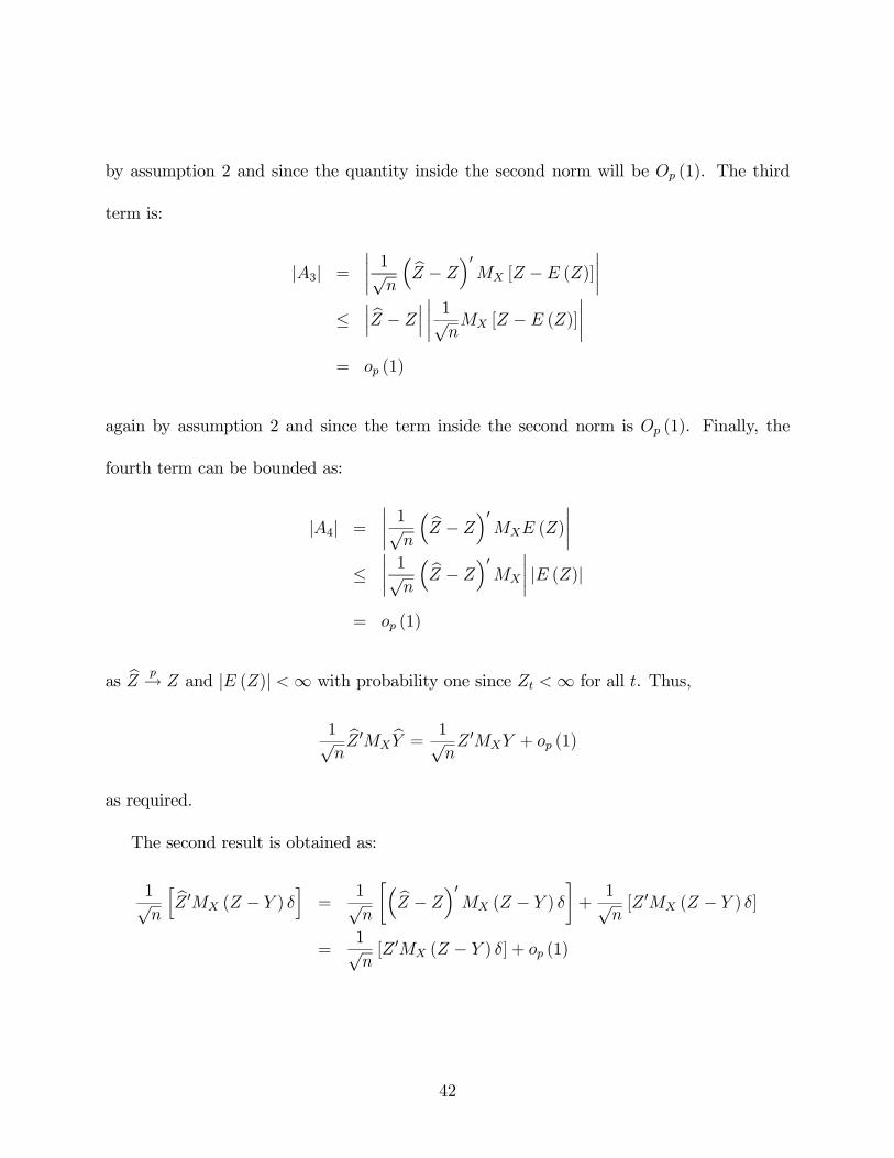
by assumption 2 and since the quantity inside the second norm will be Op (1). The third
term is:
|A3| =¯1√n
³ bZ − Z´0MX [Z −E (Z)]¯
≤¯ bZ − Z ¯ ¯ 1√
nMX [Z − E (Z)]
¯= op (1)
again by assumption 2 and since the term inside the second norm is Op (1). Finally, the
fourth term can be bounded as:
|A4| =¯1√n
³ bZ − Z´0MXE (Z)
¯≤
¯1√n
³ bZ − Z´0MX
¯|E (Z)|
= op (1)
as bZ p→ Z and |E (Z)| <∞ with probability one since Zt <∞ for all t. Thus,
1√nbZ 0MX
bY = 1√nZ 0MXY + op (1)
as required.
The second result is obtained as:
1√n
h bZ 0MX (Z − Y ) δi=
1√n
·³ bZ − Z´0MX (Z − Y ) δ¸+
1√n[Z 0MX (Z − Y ) δ]
=1√n[Z 0MX (Z − Y ) δ] + op (1)
42
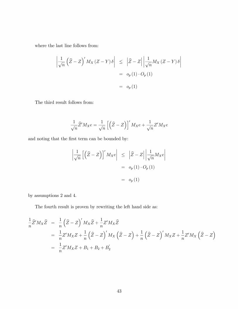
where the last line follows from:
¯1√n
³ bZ − Z´0MX (Z − Y ) δ¯≤
¯ bZ − Z ¯ ¯ 1√nMX (Z − Y ) δ
¯= op (1) ·Op (1)
= op (1)
The third result follows from:
1√nbZ 0MXe =
1√n
h³ bZ − Z´i0MXe+1√nZ 0MXe
and noting that the first term can be bounded by:
¯1√n
h³ bZ − Z´i0MXe
¯≤
¯ bZ − Z ¯ ¯ 1√nMXe
¯= op (1) ·Op (1)
= op (1)
by assumptions 2 and 4.
The fourth result is proven by rewriting the left hand side as:
1
nbZ 0MX
bZ =1
n
³ bZ − Z´0MXbZ + 1
nZ 0MX
bZ=
1
nZ 0MXZ +
1
n
³ bZ − Z´0MX
³ bZ − Z´+ 1n
³ bZ − Z´0MXZ +1
nZ 0MX
³ bZ − Z´=
1
nZ 0MXZ +B1 +B2 +B
02
43
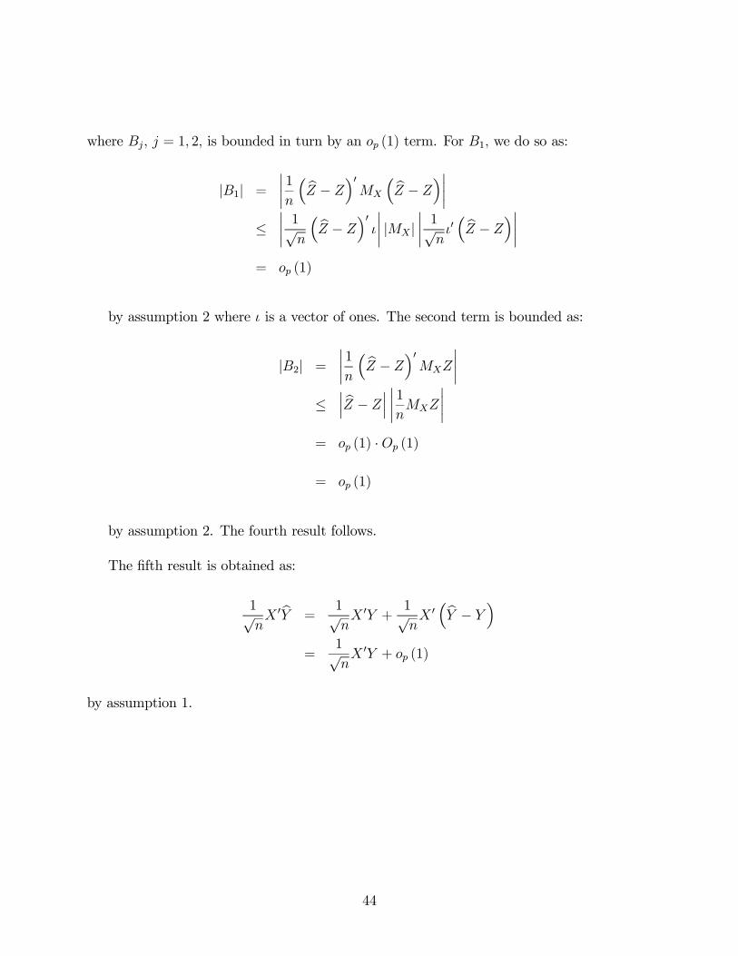
where Bj, j = 1, 2, is bounded in turn by an op (1) term. For B1, we do so as:
|B1| =¯1
n
³ bZ − Z´0MX
³ bZ − Z´¯≤
¯1√n
³ bZ − Z´0 ι¯ |MX |¯1√nι0³ bZ − Z´¯
= op (1)
by assumption 2 where ι is a vector of ones. The second term is bounded as:
|B2| =¯1
n
³ bZ − Z´0MXZ
¯≤
¯ bZ − Z ¯ ¯ 1nMXZ
¯= op (1) ·Op (1)
= op (1)
by assumption 2. The fourth result follows.
The fifth result is obtained as:
1√nX 0bY =
1√nX 0Y +
1√nX 0³bY − Y ´
=1√nX 0Y + op (1)
by assumption 1.
44
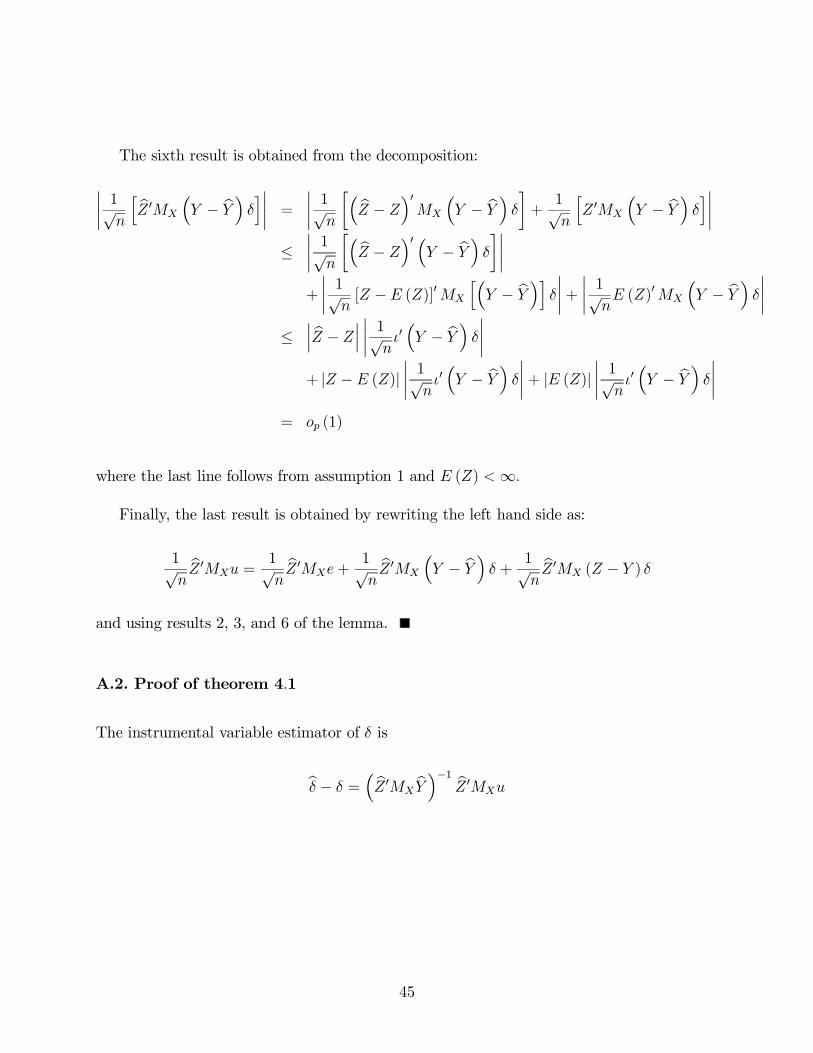
The sixth result is obtained from the decomposition:
¯1√n
h bZ 0MX
³Y − bY ´ δi¯ =
¯1√n
·³ bZ − Z´0MX
³Y − bY ´ δ¸+ 1√
n
hZ 0MX
³Y − bY ´ δi¯
≤¯1√n
·³ bZ − Z´0 ³Y − bY ´ δ¸¯+
¯1√n[Z − E (Z)]0MX
h³Y − bY ´i δ ¯+ ¯ 1√
nE (Z)0MX
³Y − bY ´ δ ¯
≤¯ bZ − Z ¯ ¯ 1√
nι0³Y − bY ´ δ ¯
+ |Z − E (Z)|¯1√nι0³Y − bY ´ δ ¯+ |E (Z)| ¯ 1√
nι0³Y − bY ´ δ ¯
= op (1)
where the last line follows from assumption 1 and E (Z) <∞.
Finally, the last result is obtained by rewriting the left hand side as:
1√nbZ 0MXu =
1√nbZ 0MXe+
1√nbZ 0MX
³Y − bY ´ δ + 1√
nbZ 0MX (Z − Y ) δ
and using results 2, 3, and 6 of the lemma.
A.2. Proof of theorem 4.1
The instrumental variable estimator of δ is
bδ − δ =³ bZ 0MX
bY ´−1 bZ 0MXu
45
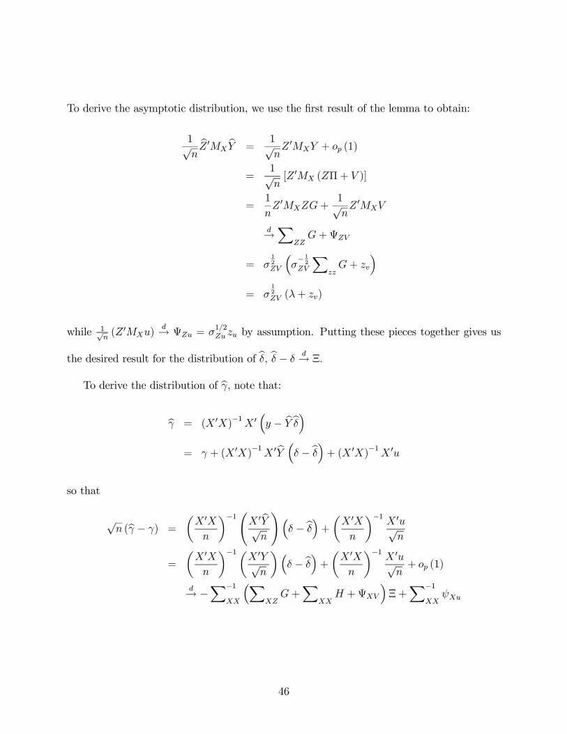
To derive the asymptotic distribution, we use the first result of the lemma to obtain:
1√nbZ 0MX
bY =1√nZ 0MXY + op (1)
=1√n[Z 0MX (ZΠ+ V )]
=1
nZ 0MXZG+
1√nZ 0MXV
d→X
ZZG+ΨZV
= σ12ZV
³σ− 12
ZV
XzzG+ zv
´= σ
12ZV (λ+ zv)
while 1√n(Z 0MXu)
d→ ΨZu = σ1/2Zu zu by assumption. Putting these pieces together gives us
the desired result for the distribution of bδ, bδ − δd→ Ξ.
To derive the distribution of bγ, note that:bγ = (X 0X)−1X 0
³y − bY bδ´
= γ + (X 0X)−1X 0bY ³δ − bδ´+ (X 0X)−1X 0u
so that
√n (bγ − γ) =
µX 0Xn
¶−1ÃX 0bY√n
!³δ − bδ´+ µX 0X
n
¶−1X 0u√n
=
µX 0Xn
¶−1µX 0Y√n
¶³δ − bδ´+ µX 0X
n
¶−1X 0u√n+ op (1)
d→ −X−1
XX
³XXZG+
XXXH +ΨXV
´Ξ+
X−1XX
ψXu
46
where the term in parentheses is derived from:
1√nX 0Y =
1√nX 0 (ZΠ+XΓ+ V )
=1
nX 0ZG+
1
nX 0XH +
1√nX 0V
d→X
XZG+
XXXH +ΨXV
by assumption.
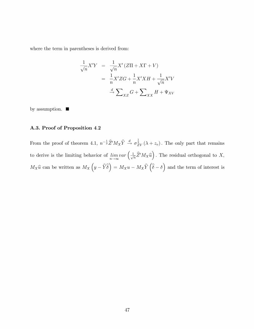
A.3. Proof of Proposition 4.2
From the proof of theorem 4.1, n−12 bZ 0MX
bY d→ σ12ZV (λ+ zv) . The only part that remains
to derive is the limiting behavior of limn→∞
var³
1√nbZ 0MXbu´ . The residual orthogonal to X,
MXbu can be written as MX
³y − bY bδ´ = MXu −MX
bY ³bδ − δ´and the term of interest is
47
therefore:
limn→∞
var
µ1√nbZ 0MXbu¶ = lim
n→∞var
µ1√nbZ 0M 0
X
hMXu−MX
bY ³bδ − δ´i¶
= limn→∞
var
µ1√n
h bZ 0M 0Xu− bZ 0M 0
XbY ³bδ − δ
´i¶= lim
n→∞var
µ1√n
hZ 0M 0
Xu− Z 0M 0X (ZΠ + V )
³bδ − δ´i+ op (1)
¶= lim
n→∞var
µ1√n
XhZ⊥t u
0t − Z⊥t Z⊥0t Π
³bδ − δ´− Z⊥t V 0t
³bδ − δ´i+ op (1)
¶= lim
n→∞1
n
Xs
XtZ⊥t u
0tusZ
⊥s
+ limn→∞
1
n
Xs
XtZ⊥t Z
⊥0t Π
³bδ − δ´³bδ − δ
´0Π0Z⊥s Z
⊥0s
+ limn→∞
1
n
Xs
XtZ⊥t V
0t
³bδ − δ´³bδ − δ
´0VsZ
⊥0s
− limn→∞
1
n
Xs
XtZ⊥t u
0t
³bδ − δ´0Π0Z⊥s Z
⊥0s
−µlimn→∞
1
n
Xs
XtZ⊥t u
0t
³bδ − δ´0Π0Z⊥s Z
⊥0s
¶0− limn→∞
1
n
Xs
XtZ⊥t u
0t
³bδ − δ´0VsZ
⊥0s
−µlimn→∞
1
n
Xs
XtZ⊥t u
0t
³bδ − δ´0VsZ
⊥0s
¶0+ limn→∞
1
n
Xs
XtZ⊥t Z
⊥0t Π
³bδ − δ´³bδ − δ
´0VsZ
⊥0s
+
µlimn→∞
1
n
Xs
XtZ⊥t Z
⊥0t Π
³bδ − δ´³bδ − δ
´0VsZ
⊥0s
¶0= σZu + C1 + C2 − C3 − C 03 − C4 − C 04 + C5 + C 05
The second term is
C1 = + limn→∞
1
n
Xs
XtZ⊥t Z
⊥0t Π
³bδ − δ´³bδ − δ
´0Π0Z⊥s Z
⊥0s
= limn→∞
1
n2
Xs
XtZ⊥t Z
⊥0t GΞΞ
0G0Z⊥s Z⊥0s
= op (1)
48
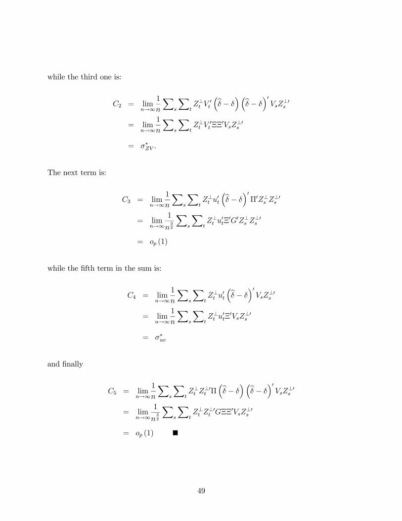
while the third one is:
C2 = limn→∞
1
n
Xs
XtZ⊥t V
0t
³bδ − δ´³bδ − δ
´0VsZ
⊥0s
= limn→∞
1
n
Xs
XtZ⊥t V
0tΞΞ
0VsZ⊥0s
= σ∗ZV .
The next term is:
C3 = limn→∞
1
n
Xs
XtZ⊥t u
0t
³bδ − δ´0Π0Z⊥s Z
⊥0s
= limn→∞
1
n32
Xs
XtZ⊥t u
0tΞ0G0Z⊥s Z
⊥0s
= op (1)
while the fifth term in the sum is:
C4 = limn→∞
1
n
Xs
XtZ⊥t u
0t
³bδ − δ´0VsZ
⊥0s
= limn→∞
1
n
Xs
XtZ⊥t u
0tΞ0VsZ⊥0s
= σ∗uv
and finally
C5 = limn→∞
1
n
Xs
XtZ⊥t Z
⊥0t Π
³bδ − δ´³bδ − δ
´0VsZ
⊥0s
= limn→∞
1
n32
Xs
XtZ⊥t Z
⊥0t GΞΞ
0VsZ⊥0s
= op (1)
49
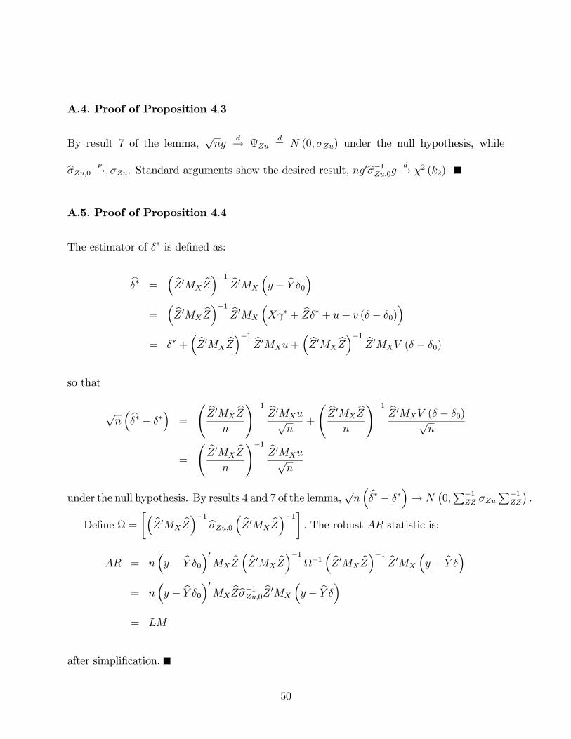
A.4. Proof of Proposition 4.3
By result 7 of the lemma,√ng
d→ ΨZud= N (0,σZu) under the null hypothesis, while
bσZu,0 p→,σZu. Standard arguments show the desired result, ng0bσ−1Zu,0g d→ χ2 (k2) .
A.5. Proof of Proposition 4.4
The estimator of δ∗ is defined as:
bδ∗ =³ bZ 0MX
bZ´−1 bZ 0MX
³y − bY δ0´
=³ bZ 0MX
bZ´−1 bZ 0MX
³Xγ∗ + bZδ∗ + u+ v (δ − δ0)
´= δ∗ +
³ bZ 0MXbZ´−1 bZ 0MXu+
³ bZ 0MXbZ´−1 bZ 0MXV (δ − δ0)
so that
√n³bδ∗ − δ∗
´=
à bZ 0MXbZ
n
!−1 bZ 0MXu√n
+
à bZ 0MXbZ
n
!−1 bZ 0MXV (δ − δ0)√n
=
à bZ 0MXbZ
n
!−1 bZ 0MXu√n
under the null hypothesis. By results 4 and 7 of the lemma,√n³bδ∗ − δ∗
´→ N
¡0,P−1
ZZ σZuP−1
ZZ
¢.
Define Ω =·³ bZ 0MX
bZ´−1 bσZu,0 ³ bZ 0MXbZ´−1¸ . The robust AR statistic is:
AR = n³y − bY δ0´0MX
bZ ³ bZ 0MXbZ´−1 Ω−1 ³ bZ 0MX
bZ´−1 bZ 0MX
³y − bY δ´
= n³y − bY δ0´0MX
bZbσ−1Zu,0 bZ 0MX
³y − bY δ´
= LM
after simplification.
50
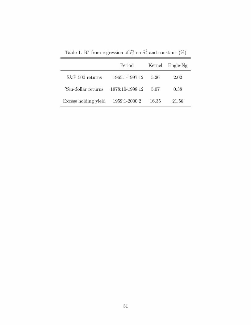
Table 1. R2 from regression of be2t on bσ2t and constant (%)Period Kernel Engle-Ng
S&P 500 returns 1965:1-1997:12 5.26 2.02
Yen-dollar returns 1978:10-1998:12 5.07 0.38
Excess holding yield 1959:1-2000:2 16.35 21.56
51
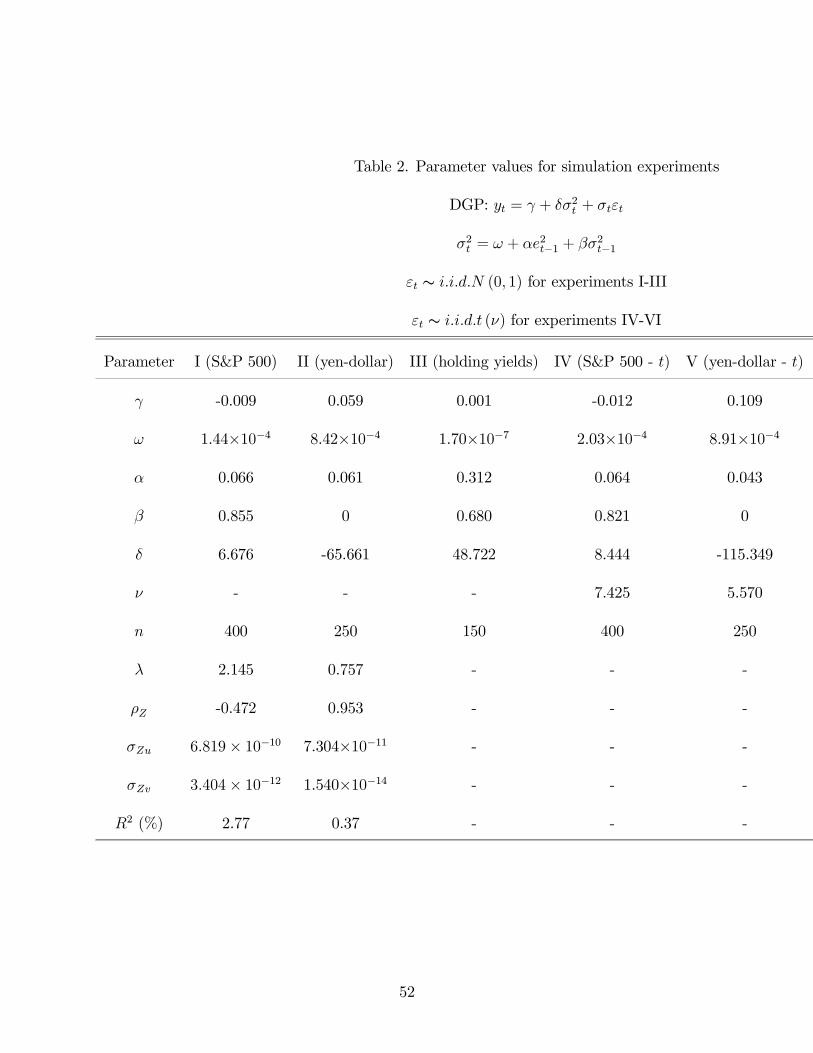
Table 2. Parameter values for simulation experiments
DGP: yt = γ + δσ2t + σtεt
σ2t = ω + αe2
t−1 + βσ2t−1
εt ∼ i.i.d.N (0, 1) for experiments I-III
εt ∼ i.i.d.t (ν) for experiments IV-VI
Parameter I (S&P 500) II (yen-dollar) III (holding yields) IV (S&P 500 - t) V (yen-dollar - t) VI (holding yields - t)
γ -0.009 0.059 0.001 -0.012 0.109 0.0005
ω 1.44×10⁻⁴ 8.42×10⁻⁴ 1.70×10⁻⁷ 2.03×10⁻⁴ 8.91×10⁻⁴ 2.03×10⁻⁷
α 0.066 0.061 0.312 0.064 0.043 0.330
β 0.855 0 0.680 0.821 0 0.651
δ 6.676 -65.661 48.722 8.444 -115.349 36.265
ν - - - 7.425 5.570 4.051
n 400 250 150 400 250 150
λ 2.145 0.757 - - - -
ρZ -0.472 0.953 - - - -
σZu 6.819 × 10⁻¹⁰ 7.304×10⁻¹¹ - - - -
σZv 3.404 × 10⁻¹² 1.540×10⁻¹⁴ - - - -
R2 (%) 2.77 0.37 - - - -
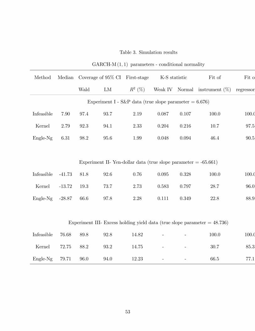
Table 3. Simulation results
GARCH-M (1, 1) parameters - conditional normality
Method Median Coverage of 95% CI First-stage K-S statistic Fit of Fit of
Wald LM R2 (%) Weak IV Normal instrument (%) regressor (%)
Experiment I - S&P data (true slope parameter = 6.676)
Infeasible 7.90 97.4 93.7 2.19 0.087 0.107 100.0 100.0
Kernel 2.79 92.3 94.1 2.33 0.204 0.216 10.7 97.5
Engle-Ng 6.31 98.2 95.6 1.99 0.048 0.094 46.4 90.5
Experiment II- Yen-dollar data (true slope parameter = -65.661)
Infeasible -41.73 81.8 92.6 0.76 0.095 0.328 100.0 100.0
Kernel -13.72 19.3 73.7 2.73 0.583 0.797 28.7 96.0
Engle-Ng -28.87 66.6 97.8 2.28 0.111 0.349 22.8 88.9
Experiment III- Excess holding yield data (true slope parameter = 48.736)
Infeasible 76.68 89.8 92.8 14.82 - - 100.0 100.0
Kernel 72.75 88.2 93.2 14.75 - - 30.7 85.3
Engle-Ng 79.71 96.0 94.0 12.23 - - 66.5 77.1
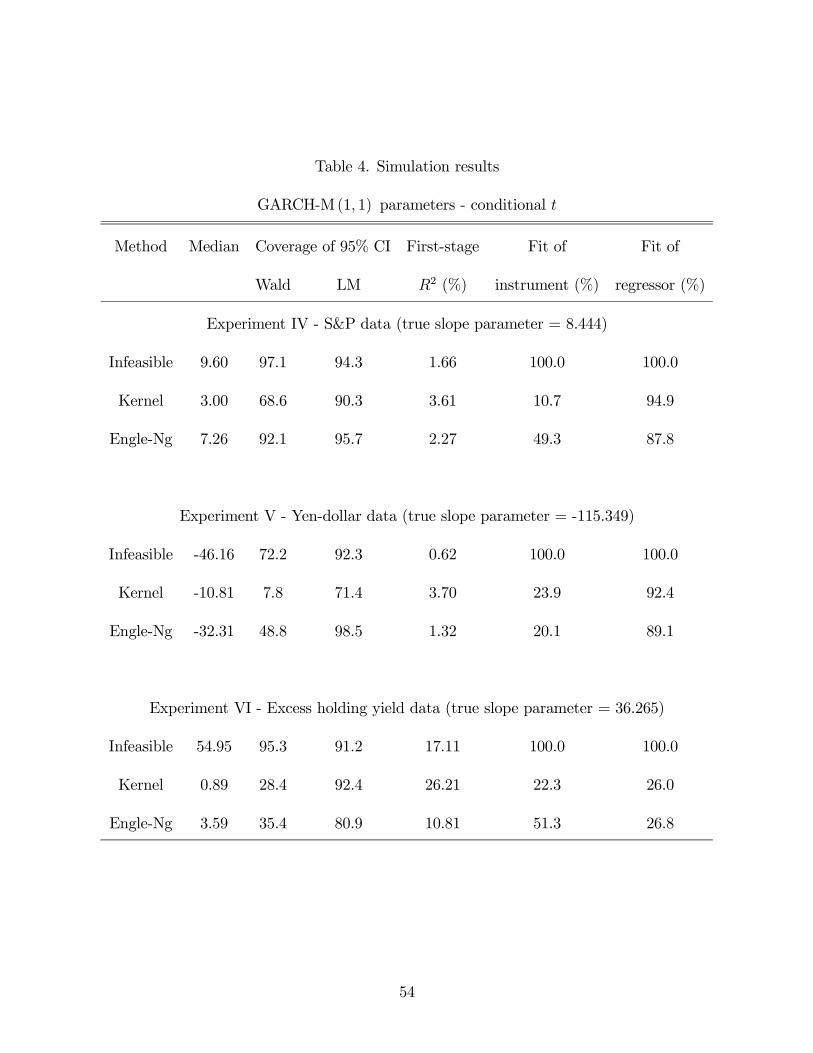
Table 4. Simulation results
GARCH-M (1, 1) parameters - conditional t
Method Median Coverage of 95% CI First-stage Fit of Fit of
Wald LM R2 (%) instrument (%) regressor (%)
Experiment IV - S&P data (true slope parameter = 8.444)
Infeasible 9.60 97.1 94.3 1.66 100.0 100.0
Kernel 3.00 68.6 90.3 3.61 10.7 94.9
Engle-Ng 7.26 92.1 95.7 2.27 49.3 87.8
Experiment V - Yen-dollar data (true slope parameter = -115.349)
Infeasible -46.16 72.2 92.3 0.62 100.0 100.0
Kernel -10.81 7.8 71.4 3.70 23.9 92.4
Engle-Ng -32.31 48.8 98.5 1.32 20.1 89.1
Experiment VI - Excess holding yield data (true slope parameter = 36.265)
Infeasible 54.95 95.3 91.2 17.11 100.0 100.0
Kernel 0.89 28.4 92.4 26.21 22.3 26.0
Engle-Ng 3.59 35.4 80.9 10.81 51.3 26.8
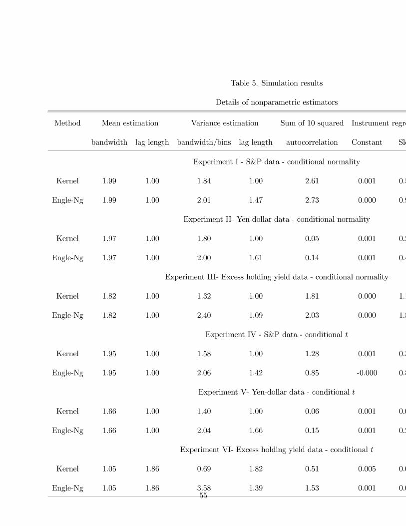
Table 5. Simulation results
Details of nonparametric estimators
Method Mean estimation Variance estimation Sum of 10 squared Instrument regression Regressor regression
bandwidth lag length bandwidth/bins lag length autocorrelation Constant Slope Constant Slope
Experiment I - S&P data - conditional normality
Kernel 1.99 1.00 1.84 1.00 2.61 0.001 0.532 0.000 1.000
Engle-Ng 1.99 1.00 2.01 1.47 2.73 0.000 0.991 0.000 1.023
Experiment II- Yen-dollar data - conditional normality
Kernel 1.97 1.00 1.80 1.00 0.05 0.001 0.252 0.000 0.990
Engle-Ng 1.97 1.00 2.00 1.61 0.14 0.001 0.447 0.000 1.040
Experiment III- Excess holding yield data - conditional normality
Kernel 1.82 1.00 1.32 1.00 1.81 0.000 1.141 0.000 1.013
Engle-Ng 1.82 1.00 2.40 1.09 2.03 0.000 1.899 0.000 1.041
Experiment IV - S&P data - conditional t
Kernel 1.95 1.00 1.58 1.00 1.28 0.001 0.300 0.000 0.997
Engle-Ng 1.95 1.00 2.06 1.42 0.85 -0.000 0.879 0.000 1.027
Experiment V- Yen-dollar data - conditional t
Kernel 1.66 1.00 1.40 1.00 0.06 0.001 0.065 0.000 0.986
Engle-Ng 1.66 1.00 2.04 1.66 0.15 0.001 0.248 0.000 1.057
Experiment VI- Excess holding yield data - conditional t
Kernel 1.05 1.86 0.69 1.82 0.51 0.005 0.015 0.007 0.015
Engle-Ng 1.05 1.86 3.58 1.39 1.53 0.001 0.078 0.007 0.018
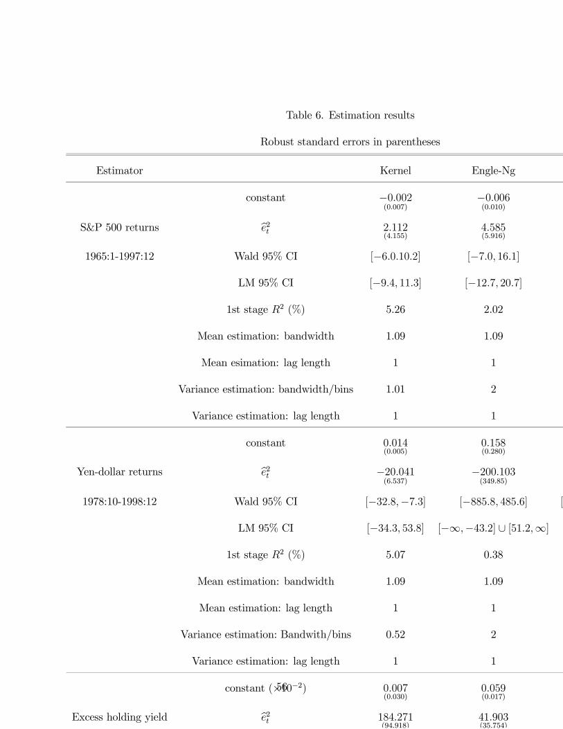
Table 6. Estimation results
Robust standard errors in parentheses
Estimator Kernel Engle-Ng GARCH-M
constant ¡0:002(0:007)
¡0:006(0:010)
¡0:009(0:010)
S&P 500 returns be2t 2:112
(4:155)4:585(5:916)
6:676(5:852)
1965:1-1997:12 Wald 95% CI [¡6:0:10:2] [¡7:0;16:1] [¡4:8;18:1]
LM 95% CI [¡9:4;11:3] [¡12:7;20:7]
1st stage R2 (%) 5.26 2.02
Mean estimation: bandwidth 1.09 1.09
Mean esimation: lag length 1 1
Variance estimation: bandwidth/bins 1.01 2
Variance estimation: lag length 1 1
constant 0:014(0:005)
0:158(0:280)
0:059(0:087)
Yen-dollar returns be2t ¡20:041
(6:537)¡200:103
(349:85)¡65:661(98:284)
1978:10-1998:12 Wald 95% CI [¡32:8;¡7:3] [¡885:8;485:6] [¡240:2; 145:1]
LM 95% CI [¡34:3; 53:8] [¡1; ¡43:2] [ [51:2; 1]
1st stage R2 (%) 5.07 0.38
Mean estimation: bandwidth 1.09 1.09
Mean estimation: lag length 1 1
Variance estimation: Bandwith/bins 0.52 2
Variance estimation: lag length 1 1
constant¡£10¡2¢ 0:007
(0:030)0:059(0:017)
0:001(0:001)
Excess holding yield be2t 184:271
(94:918)41:903(35:754)
48:722(16:508)
1959:1-2000:2 Wald 95% CI [¡1:7;370:3] [¡28:1;111:9] [16:4;81:1]
LM 95% CI [¡1000; 1000] [¡235:4;110:3]
1st stage R2 (%) 16.35 21.56
Mean estimation: bandwidth 0.28 0.28
Mean estimation: lag length 1 1
Variance estimation: bandwidth/bins 0.06 4
Variance estimation: lag length 1 1


![SCANNING TUTORIAL - PARSONS SSCE · SCANNING TUTORIAL. open EPSON scan utility on desktop. select Professional Mode. ... OptiTex Adobe Acrobat Distiller X] Adobe …](https://img.pdfslide.us/doc/110x75/5b7704017f8b9a515a8c24df/scanning-tutorial-parsons-ssce-scanning-tutorial-open-epson-scan-utility.jpg)