Acquisition method improvement for Bossa Nova Technologies ... · using Bossa Nova Technologies full Stokes polarization imaging. 1.1 Background Along with the intensity and the spectrum,

Acquisition method improvement for Bossa Nova Technologies' full Stokes, passive polarization imaging camera SALSA

M. EL KETARAa, M. Vedela and S. Breugnota

aBossa Nova Technologies, 11922 Jefferson Blvd., Culver city, CA 90230, USA

ABSTRACT

For some applications, the need for fast polarization acquisition is essential (if the scene observed is moving or changing quickly). In this paper, we present a new acquisition method for Bossa Nova Technologies’ full Stokes passive polarization imaging camera, the SALSA. This polarization imaging camera is based on “Division of Time polarimetry” architecture. The use of this technique presents the advantage of preserving the full resolution of the image observed all the while reducing the speed acquisition time. The goal of this new acquisition method is to overcome the limitations associated with Division of Time acquisition technique as well as to obtain high-speed polarization imaging while maintaining the image resolution. The efficiency of this new method is demonstrated in this paper through different experiments.

Keywords: Division-of-time polarimeter, polarization, imaging, Full Stokes, fast acquisition, Time translation.

1. INTRODUCTION In this paper, we will present a method to recover full polarization information in high resolution with high frame rate using Bossa Nova Technologies’ full Stokes polarization imaging.

1.1 Background

Along with the intensity and the spectrum, the polarization of light carries abundant information.

A common representation used to describe completely any partial or total polarization state is the Stokes formalism [1]:

S (x,y) =

⎟⎟⎟⎟⎟

⎠

⎞

⎜⎜⎜⎜⎜

⎝

⎛

3

2

1

0

SSSS

(1)

with S0 the total intensity of light detected by the camera, S1 the difference in intensities between the horizontal and vertical linearly polarized components, S2 the difference in intensities between linearly polarized components traveling at 45° and −45° based on the x-axis; S3 the difference in intensities between right and left circularly polarized light.

From this vector, a wide variety of information can be gathered such as:

- The total intensity S0 which corresponds to what will be seen by a regular camera

- The degree of polarization (DOP) provides a measurement of the ratio of polarized light relative to the total amount of light received. However, it is not possible to differentiate linear from elliptical or circular polarization using just this parameter

- The degree of linear polarization (DOLP) provides a measurement of the ratio of linearly polarized light relative to the total amount of light received

Polarization: Measurement, Analysis, and Remote Sensing XII, edited by David B. Chenault, Dennis H. Goldstein, Proc. of SPIE Vol. 9853, 98530A · © 2016 SPIE · CCC code: 0277-786X/16/$18 · doi: 10.1117/12.2224357

Proc. of SPIE Vol. 9853 98530A-1

Downloaded From: http://proceedings.spiedigitallibrary.org/ on 10/03/2016 Terms of Use: http://spiedigitallibrary.org/ss/termsofuse.aspx

OTOic2f linrC?

km

Dolarization terra

- The degree of circular polarization (DOCP) provides a measurement of the ratio of circularly polarized light relative to the total amount of light received

- The angle of polarization (AOP): when light is partially or totally linearly polarized it corresponds to the angle of orientation associated to the polarization ellipse

- The ellipticity (EPS): when light is partially or totally linearly polarized it corresponds to the ellipticity associated with the polarization ellipse

While most of the available polarization imaging cameras perform only linear Stokes polarization imaging (only the linear polarization can be quantified) due to their technological limitation, the SALSA system performs live measurement of the full Stokes vector for each pixel (S0, S1, S2, S3) of the image with high resolution. This system is based on a division of time polarimeter architecture using ferroelectric liquid crystals specially optimized for the visible range [2-4].

1.2 Division of time polarimeter architecture

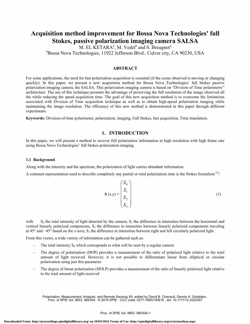
The first polarization imaging systems were division-of-time polarimeters[5] using mechanical rotation of the polarizer(s) and waveplate(s) between each frame. These systems are usually quite slow and are very sensitive to the scene or target moving between frames. To reconstruct full polarization information, the imaging system usually required the acquisition of 4 consecutives raw images in order to compute the corresponding Stokes vector for each pixel of the scene (Figure 1).

Figure 1: Example of polarized glasses imaged with a division of time polarimeter architecture device.

The assumption made when using this technique is that the physical object observed has the same features over the interval of time required to capture the four images. Only if the polarization system imaging switches quickly between the four raw images compared to the scene modification does this prove to be true.

During the course of a previous study [3], we presented an integrated faster polarization imaging system using liquid crystal technology to acquire the 4 images necessary using division of time polarimetry architecture[5]. Thanks to this patented technique, the system can easily be adapted to any imaging system without spatial misregistration or resolution loss (compared to imaging alone). This method also allows the user to gather the circular and elliptical polarization light information.

Three main issues arise when using division of polarimeter architecture. The first is the time required to capture one polarization image: the polarization frame rate is four times slower than the imaging sensor’s frame rate. The other is linked to the visualization system: in case of high frame rates, the camera itself may drop images. The last is linked to



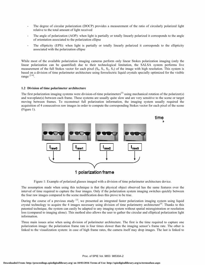
the acquisition system (the computer): due to other processes required of the acquisition system (data saving, display and others), the number of frames effectively saved is less than expected (Table 1).

Image 1 2 3 4 5 6 7 8 9 10 11 12 13 14 15 16 17 18 19 20

Raw image successfully

acquired

0

1

2

3

0

1

Raw not sent

3

0

1

2

3

0

1

2

3

0

1

2

3

Polarization frame

succesfully acquired

1

Frame cannot be acquired (camera)

2

Frame cannot be acquired (computer)

3

Table 1. Schematic representation of polarization frame rate limitation.

The methods identified to solve these three main issues are introduced in the following section.

2. FAST POLARIZATION IMAGING METHOD

2.1 Camera-computer connection

As previously established, the first step is to ensure that all raw images are successfully acquired. This is accomplished by selecting the proper camera bus and resending data when errors occur during transmission.

Many camera bus exist on the market all of which have advantages and limitations depending on the application (Table 2).

Data transfer rate

Maximum cable length

Possibility to plug to basic computer

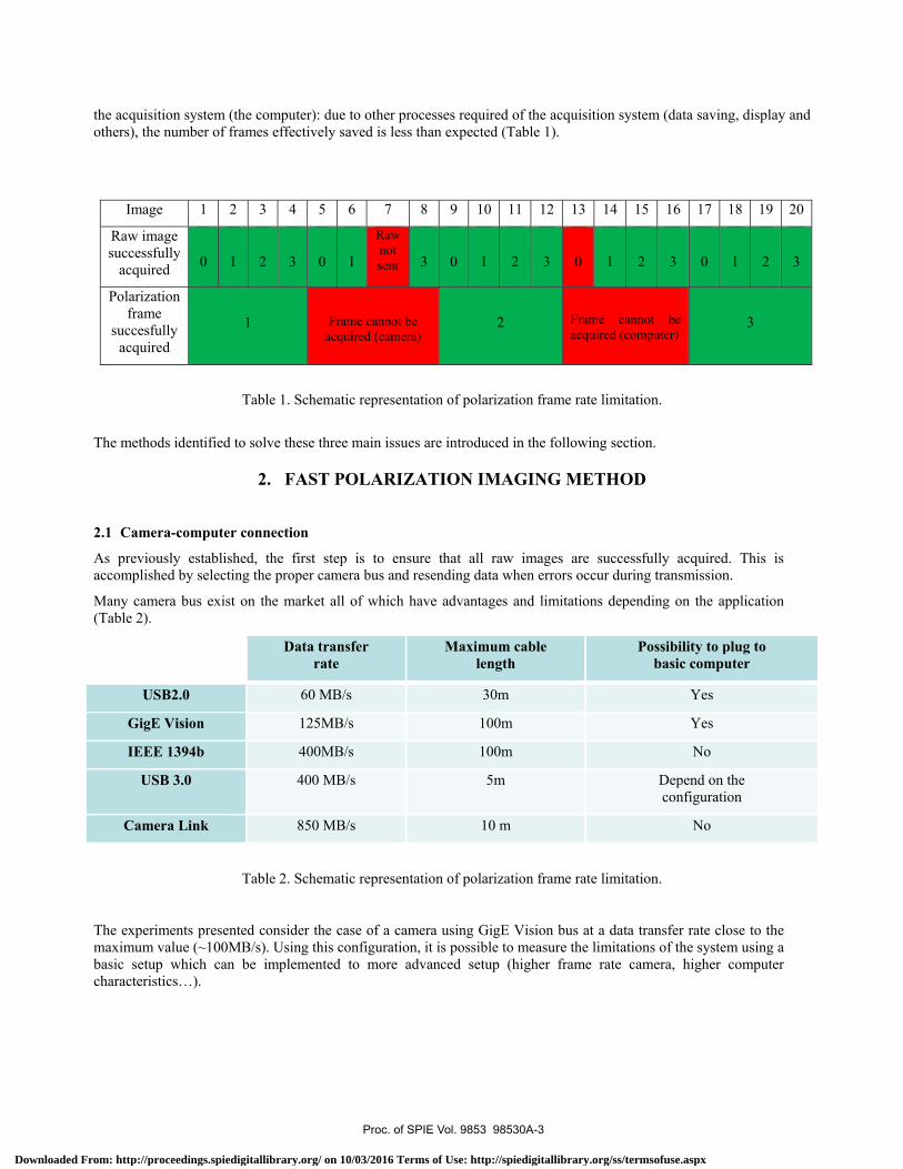
USB2.0 60 MB/s 30m Yes

GigE Vision 125MB/s 100m Yes

IEEE 1394b 400MB/s 100m No

USB 3.0 400 MB/s 5m Depend on the configuration

Camera Link 850 MB/s 10 m No

Table 2. Schematic representation of polarization frame rate limitation.

The experiments presented consider the case of a camera using GigE Vision bus at a data transfer rate close to the maximum value (~100MB/s). Using this configuration, it is possible to measure the limitations of the system using a basic setup which can be implemented to more advanced setup (higher frame rate camera, higher computer characteristics…).



time

Sensor frames (FPS = f)

:Raw image

Polarization frameacquisition Withprevious method

(FPS =f /4)

3 10 13 14 15 16 IS 19

3 4 3 4 3

Sensor frames (FPS = f) l

Polarization frameacquisi.tiou. witù.. .

new method

(FPS = i)

1'134Frame 1

dt

20

Frame 2Frame 3

Frame 4Frame 5

Frame 6Frame 7

Frame 8Frame 9

Frame 10Frame 11

Frame 12Frame 13

Frame 14Frame 15

Frame 16Frame 17

2.2 Method to increase the polarization frame rate

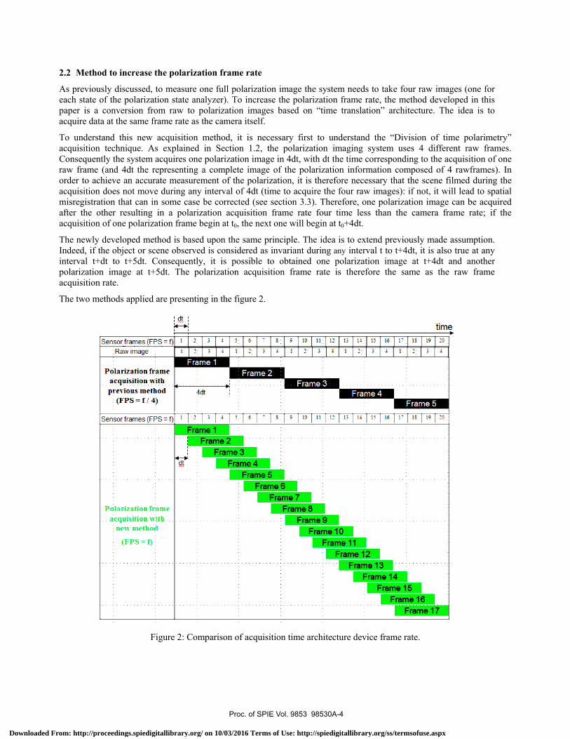
As previously discussed, to measure one full polarization image the system needs to take four raw images (one for each state of the polarization state analyzer). To increase the polarization frame rate, the method developed in this paper is a conversion from raw to polarization images based on “time translation” architecture. The idea is to acquire data at the same frame rate as the camera itself.

To understand this new acquisition method, it is necessary first to understand the “Division of time polarimetry” acquisition technique. As explained in Section 1.2, the polarization imaging system uses 4 different raw frames. Consequently the system acquires one polarization image in 4dt, with dt the time corresponding to the acquisition of one raw frame (and 4dt the representing a complete image of the polarization information composed of 4 rawframes). In order to achieve an accurate measurement of the polarization, it is therefore necessary that the scene filmed during the acquisition does not move during any interval of 4dt (time to acquire the four raw images): if not, it will lead to spatial misregistration that can in some case be corrected (see section 3.3). Therefore, one polarization image can be acquired after the other resulting in a polarization acquisition frame rate four time less than the camera frame rate; if the acquisition of one polarization frame begin at t0, the next one will begin at t0+4dt.

The newly developed method is based upon the same principle. The idea is to extend previously made assumption. Indeed, if the object or scene observed is considered as invariant during any interval t to t+4dt, it is also true at any interval t+dt to t+5dt. Consequently, it is possible to obtained one polarization image at t+4dt and another polarization image at t+5dt. The polarization acquisition frame rate is therefore the same as the raw frame acquisition rate.

The two methods applied are presenting in the figure 2.

Figure 2: Comparison of acquisition time architecture device frame rate.



<=1Sampleplate

Rotatingstage <=1

Non -polarizedlight

Polarizer plates1 plates

Elliptical plate

fir0 ö ó ó E é S ó ó 8 8

$ $t rS o ó S S ó

® ® ® o

oon-0

Do-c)

Using this method, the Division of time polarimeter system can acquire data at the same frame rate as the camera itself.

3. FAST POLARIZATION IMAGING ACQUISITION

3.1 Validation of polarimeter efficiency in video mode: rotation experimental protocol

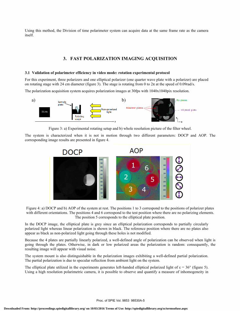
For this experiment, three polarizers and one elliptical polarizer (one quarter wave plate with a polarizer) are placed on rotating stage with 24 cm diameter (figure 3). The stage is rotating from 0 to 2π at the speed of 0.09rad/s.

The polarization acquisition system acquires polarization images at 30fps with 1040x1040pix resolution.

Figure 3: a) Experimental rotating setup and b) whole resolution picture of the filter wheel.

The system is characterized when it is not in motion through two different parameters: DOCP and AOP. The corresponding image results are presented in figure 4.

Figure 4: a) DOCP and b) AOP of the system at rest. The positions 1 to 3 correspond to the positions of polarizer plates with different orientations. The positions 4 and 6 correspond to the test position where there are no polarizing elements.

The position 5 corresponds to the elliptical plate position.

In the DOCP image, the elliptical plate is grey since an elliptical polarization corresponds to partially circularly polarized light whereas linear polarization is shown in black. The reference position where there are no plates also appear as black as non-polarized light going through these holes is not modified.

Because the 4 plates are partially linearly polarized, a well-defined angle of polarization can be observed when light is going through the plates. Otherwise, in dark or low polarized areas the polarization is random: consequently, the resulting image will appear with visual noise.

The system mount is also distinguishable in the polarization images exhibiting a well-defined partial polarization. The partial polarization is due to specular reflection from ambient light on the system.

The elliptical plate utilized in the experiments generates left-handed elliptical polarized light of ε = 36° (figure 5). Using a high resolution polarimetric camera, it is possible to observe and quantify a measure of inhomogeneity in

b) a)



AOP EPS Polarization ellipse

Arro

.°`

360

310

260

210

160

110

dig!.IÍil''';,;olluüüiIiI1111110111111111111IIIII ÌIIIiiiÍ, II Illli ...,IIlíll.:..-

. film 60 I11N''1111Ii jIIIIIIIII%E:i1111111111'I;iiiii' !1_r.:¡'=__-- 1 III.N . -_.:...II II1111IIIhuIIIPII Ilq:nuupnl

140Rotation angle (in degree)

t ElliticaI plate

Polar 1

- Polar 2

--I--- Polar 3

- No plate 1

No plate 2

Theory

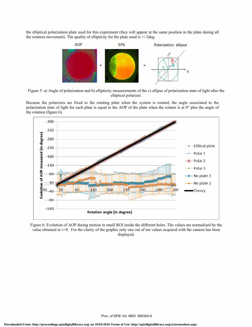
the elliptical polarization plate used for this experiment (they will appear at the same position in the plate during all the rotation movement). The quality of ellipticity for the plate used is +/-2deg.

Figure 5: a) Angle of polarization and b) ellipticity measurements of the c) ellipse of polarization state of light after the

elliptical polarizer.

Because the polarizers are fixed to the rotating plate when the system is rotated, the angle associated to the polarization state of light for each plate is equal to the AOP of the plate when the rotator is at 0° plus the angle of the rotation (figure 6).

Figure 6: Evolution of AOP during motion in small ROI inside the different holes. The values are normalized by the value obtained at v=0. For the clarity of the graphic only one out of ten values acquired with the camera has been

displayed.



Salsa

Sample plate

Translationstage along x

Non- polarizedlight

<=1>z

Edge effects

AOP (sample moving: v= 200mm /s) AOP (system at rest: v =0)

EPS (sample moving: v= 200mm /s) EPS (system at rest: v =0)

90

0

90

-45

Region of inteobserved

est

Polarizer platePolarizer diameter =5em

Y ®x 400 GOO 700 003 000 1000

Illumination

Translation stage

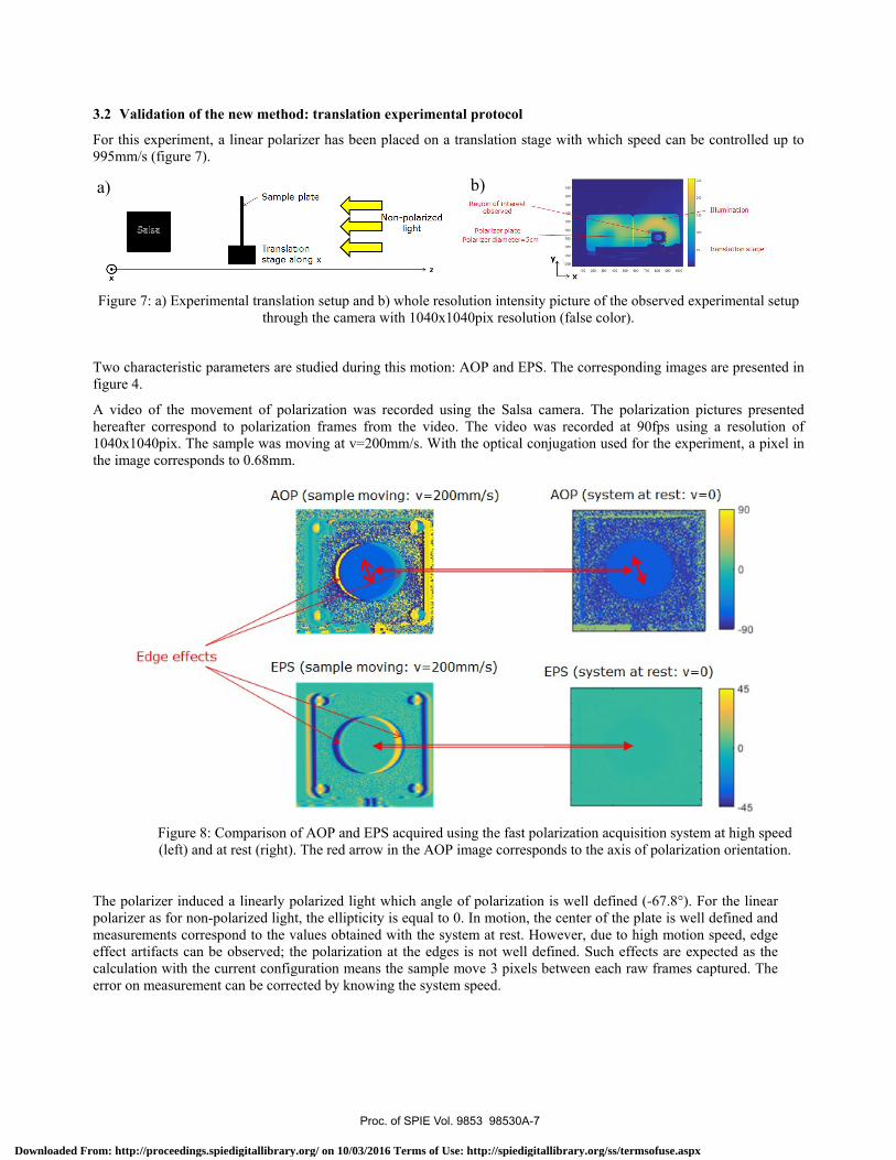
3.2 Validation of the new method: translation experimental protocol

For this experiment, a linear polarizer has been placed on a translation stage with which speed can be controlled up to 995mm/s (figure 7).

Figure 7: a) Experimental translation setup and b) whole resolution intensity picture of the observed experimental setup

through the camera with 1040x1040pix resolution (false color).

Two characteristic parameters are studied during this motion: AOP and EPS. The corresponding images are presented in figure 4.

A video of the movement of polarization was recorded using the Salsa camera. The polarization pictures presented hereafter correspond to polarization frames from the video. The video was recorded at 90fps using a resolution of 1040x1040pix. The sample was moving at v=200mm/s. With the optical conjugation used for the experiment, a pixel in the image corresponds to 0.68mm.

Figure 8: Comparison of AOP and EPS acquired using the fast polarization acquisition system at high speed (left) and at rest (right). The red arrow in the AOP image corresponds to the axis of polarization orientation.

The polarizer induced a linearly polarized light which angle of polarization is well defined (-67.8°). For the linear polarizer as for non-polarized light, the ellipticity is equal to 0. In motion, the center of the plate is well defined and measurements correspond to the values obtained with the system at rest. However, due to high motion speed, edge effect artifacts can be observed; the polarization at the edges is not well defined. Such effects are expected as the calculation with the current configuration means the sample move 3 pixels between each raw frames captured. The error on measurement can be corrected by knowing the system speed.

b) a)



Raw 1 Raw 2

IdgPolarization image recovered

Misregistration

Raw 3 Raw 4

Expected polarization image

Exposuretime

Readouttime

TimeY

Camera frame acquisition

dt

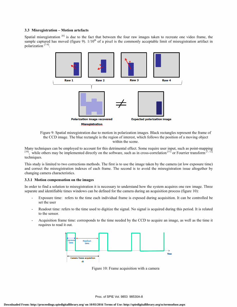
3.3 Misregistration – Motion artefacts

Spatial misregistration [6] is due to the fact that between the four raw images taken to recreate one video frame, the sample captured has moved (figure 9). 1/10th of a pixel is the commonly acceptable limit of misregistration artifact in polarization [7-9].

Figure 9: Spatial misregistration due to motion in polarization images. Black rectangles represent the frame of

the CCD image. The blue rectangle is the region of interest, which follows the position of a moving object within the scene.

Many techniques can be employed to account for this detrimental effect. Some require user input, such as point-mapping [10], while others may be implemented directly on the software, such as in cross-correlation [11] or Fourrier transform [7, 12] techniques.

This study is limited to two corrections methods. The first is to use the image taken by the camera (at low exposure time) and correct the misregistration indexes of each frame. The second is to avoid the misregistration issue altogether by changing camera characteristics.

3.3.1 Motion compensation on the images

In order to find a solution to misregistration it is necessary to understand how the system acquires one raw image. Three separate and identifiable times windows can be defined for the camera during an acquisition process (figure 10):

- Exposure time: refers to the time each individual frame is exposed during acquisition. It can be controlled be set the user

- Readout time: refers to the time used to digitize the signal. No signal is acquired during this period. It is related to the sensor.

- Acquisition frame time: corresponds to the time needed by the CCD to acquire an image, as well as the time it requires to read it out.

Figure 10: Frame acquisition with a camera



Raw frame acquired

Motion compensation

(displacement of pixels associated

to region of interest)

Raw 1 Raw 2 Raw 3

Polarization imagecorrected

Raw 4

".

Atv3_v2

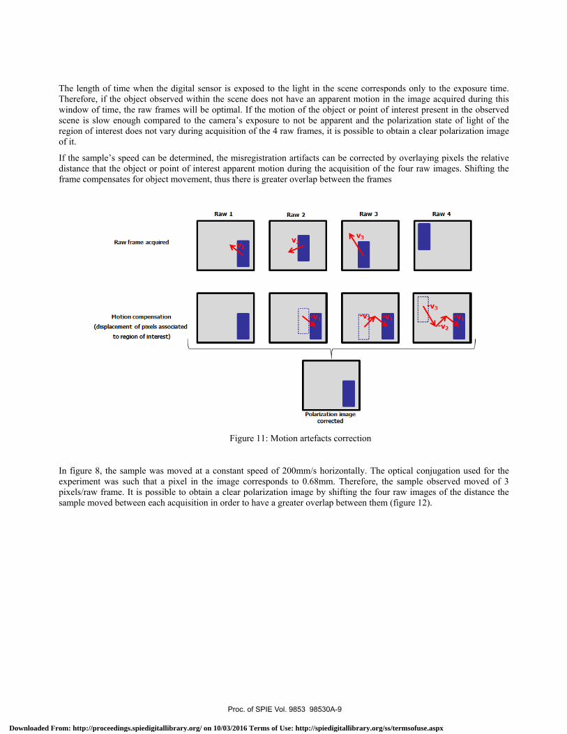
The length of time when the digital sensor is exposed to the light in the scene corresponds only to the exposure time. Therefore, if the object observed within the scene does not have an apparent motion in the image acquired during this window of time, the raw frames will be optimal. If the motion of the object or point of interest present in the observed scene is slow enough compared to the camera’s exposure to not be apparent and the polarization state of light of the region of interest does not vary during acquisition of the 4 raw frames, it is possible to obtain a clear polarization image of it.

If the sample’s speed can be determined, the misregistration artifacts can be corrected by overlaying pixels the relative distance that the object or point of interest apparent motion during the acquisition of the four raw images. Shifting the frame compensates for object movement, thus there is greater overlap between the frames

Figure 11: Motion artefacts correction

In figure 8, the sample was moved at a constant speed of 200mm/s horizontally. The optical conjugation used for the experiment was such that a pixel in the image corresponds to 0.68mm. Therefore, the sample observed moved of 3 pixels/raw frame. It is possible to obtain a clear polarization image by shifting the four raw images of the distance the sample moved between each acquisition in order to have a greater overlap between them (figure 12).



i

OfIP with misregistration correction90

40

EPS with misregistration correction45

0

45

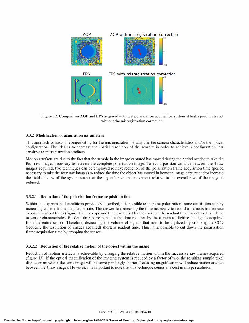
Figure 12: Comparison AOP and EPS acquired with fast polarization acquisition system at high speed with and

without the misregistration correction

3.3.2 Modification of acquisition parameters

This approach consists in compensating for the misregistration by adapting the camera characteristics and/or the optical configuration. The idea is to decrease the spatial resolution of the sensory in order to achieve a configuration less sensitive to misregistration artefacts.

Motion artefacts are due to the fact that the sample in the image captured has moved during the period needed to take the four raw images necessary to recreate the complete polarization image. To avoid position variance between the 4 raw images acquired, two techniques can be employed jointly: reduction of the polarization frame acquisition time (period necessary to take the four raw images) to reduce the time the object has moved in between image capture and/or increase the field of view of the system such that the object’s size and movement relative to the overall size of the image is reduced.

3.3.2.1 Reduction of the polarization frame acquisition time

Within the experimental conditions previously described, it is possible to increase polarization frame acquisition rate by increasing camera frame acquisition rate. The answer to decreasing the time necessary to record a frame is to decrease exposure readout times (figure 10). The exposure time can be set by the user, but the readout time cannot as it is related to sensor characteristics. Readout time corresponds to the time required by the camera to digitize the signals acquired from the entire sensor. Therefore, decreasing the volume of signals that need to be digitized by cropping the CCD (reducing the resolution of images acquired) shortens readout time. Thus, it is possible to cut down the polarization frame acquisition time by cropping the sensor.

3.3.2.2 Reduction of the relative motion of the object within the image

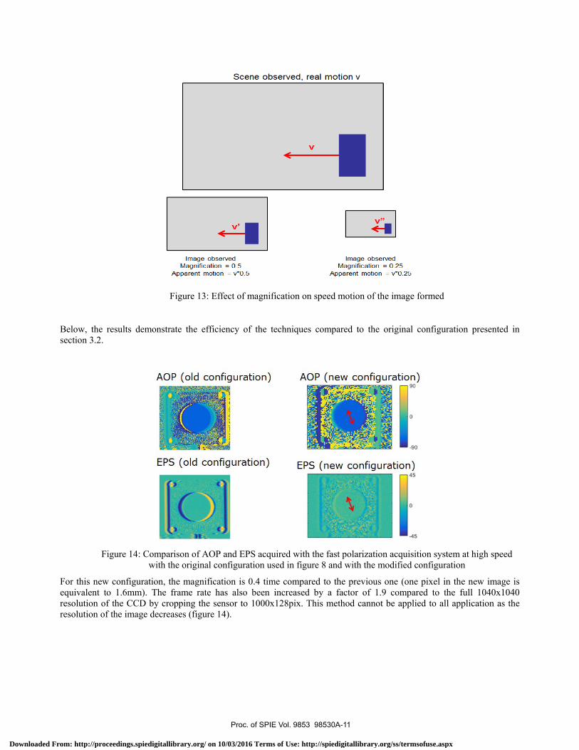
Reduction of motion artefacts is achievable by changing the relative motion within the successive raw frames acquired (figure 13). If the optical magnification of the imaging system is reduced by a factor of two, the resulting sample pixel displacement within the same image will be correspondingly shorter. Reducing magnification will reduce motion artefact between the 4 raw images. However, it is important to note that this technique comes at a cost in image resolution.



AOP (old configuration)

EPS (old configuration)

li

AOP (new configuration)90

0

90

EPS (new configuration)45

0

-45

Scene observed, real motion v

Image observedMagnification = 0.5

Apparent motion = v *0.5

Image observedMagnification = 0.25

Apparent motion = v *0.25

Figure 13: Effect of magnification on speed motion of the image formed

Below, the results demonstrate the efficiency of the techniques compared to the original configuration presented in section 3.2.

Figure 14: Comparison of AOP and EPS acquired with the fast polarization acquisition system at high speed

with the original configuration used in figure 8 and with the modified configuration

For this new configuration, the magnification is 0.4 time compared to the previous one (one pixel in the new image is equivalent to 1.6mm). The frame rate has also been increased by a factor of 1.9 compared to the full 1040x1040 resolution of the CCD by cropping the sensor to 1000x128pix. This method cannot be applied to all application as the resolution of the image decreases (figure 14).



Polarized light

Unstressed plasticSame polarization and

spatially homogeneous light

Modification of polarization:

Elliptical polarization and

spatially inhomogeneous light'Iy

nl I

Polarized light

1n

Stressed plastic

Salsa

Intensity

1cm

AOP (v=0)

EPS_(v=0)

AOP (v=200mm/s) AOP (v=500mm/s) AOP (v=995mm/s)

900

.yo

EPS (v=200mm/s) EPS (v=500mm/s) EPS (v=995mm/s)

1 o

-4SV

4. APPLICATION TO THE STUDY OF A STRESS SAMPLE IN MOTION

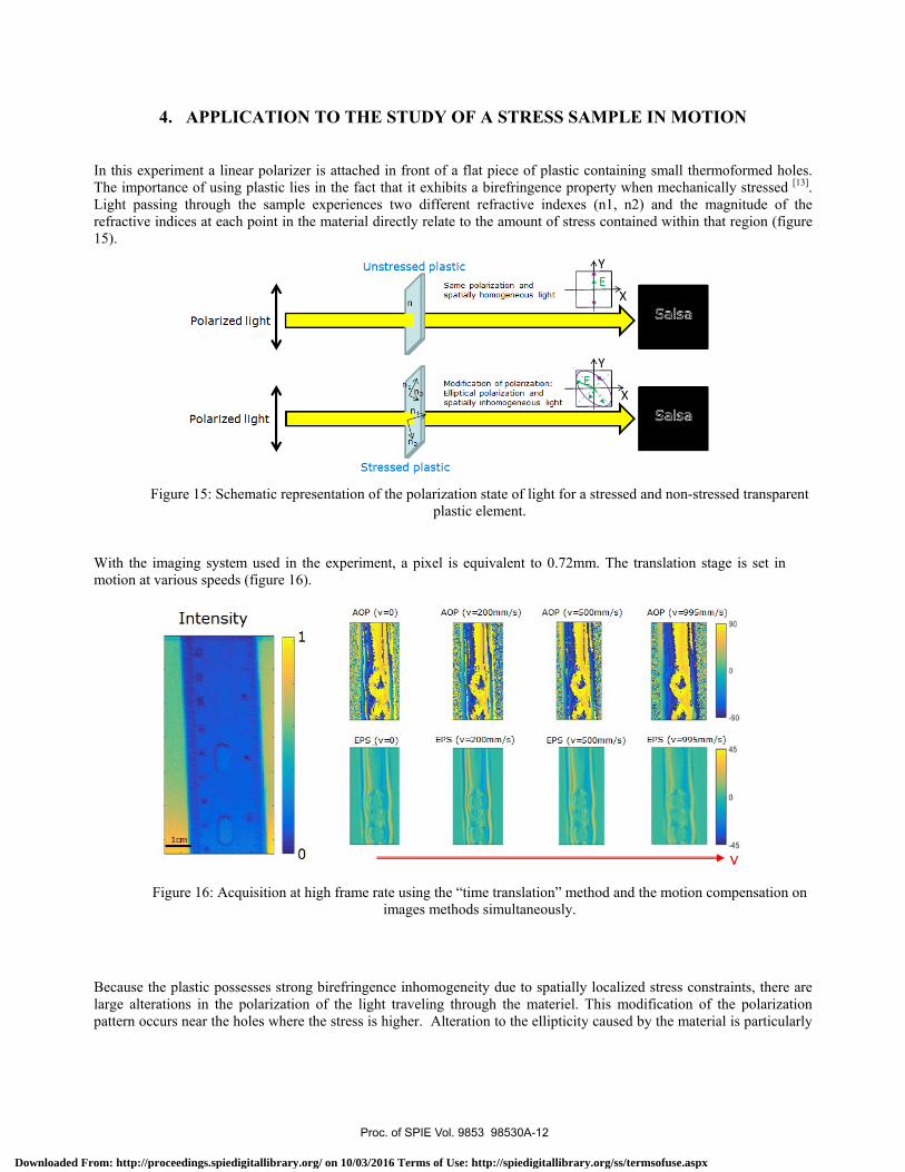
In this experiment a linear polarizer is attached in front of a flat piece of plastic containing small thermoformed holes. The importance of using plastic lies in the fact that it exhibits a birefringence property when mechanically stressed [13]. Light passing through the sample experiences two different refractive indexes (n1, n2) and the magnitude of the refractive indices at each point in the material directly relate to the amount of stress contained within that region (figure 15).

Figure 15: Schematic representation of the polarization state of light for a stressed and non-stressed transparent

plastic element.

With the imaging system used in the experiment, a pixel is equivalent to 0.72mm. The translation stage is set in motion at various speeds (figure 16).

Figure 16: Acquisition at high frame rate using the “time translation” method and the motion compensation on

images methods simultaneously.

Because the plastic possesses strong birefringence inhomogeneity due to spatially localized stress constraints, there are large alterations in the polarization of the light traveling through the materiel. This modification of the polarization pattern occurs near the holes where the stress is higher. Alteration to the ellipticity caused by the material is particularly



TtG

_tive time Average response time

82% 385 msR

O KB /strite

speed

2.9 MB/s

Capacity: 466 G6

Fo imatted: 466 G6

System disk: Yes

Page file: Ves

interesting as the stress pattern can be observed more clearly than in the angle of polarization (linear Stokes parameters usually being the only observable parameter measured by polarization camera).

5. DISCUSSION As demonstrated, high speed acquisition with high resolution can be performed using this new Salsa camera method. However, there are issues during long acquisitions which are discussed below.

The memory usage increased progressively during the saving process at 90fps in the configuration used; 1040x1040 pix resolution Salsa camera and a computer with the following characteristics: Dual Core CPU 3GHz, 6GB Ram, HDD: SATA II).

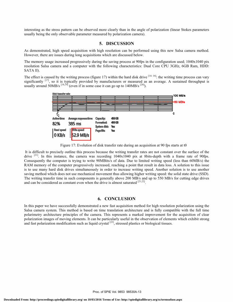
The effect is caused by the writing process (figure 17) within the hard disk drive [14- 16]: the writing time process can vary significantly [17], so it is typically provided by manufacturers or measured as an average. A sustained throughput is usually around 50MB/s [18,19] (even if in some case it can go up to 140MB/s [20]).

Figure 17: Evolution of disk transfer rate during an acquisition at 90 fps starts at t0

It is difficult to precisely outline this process because the writing transfer rates are not constant over the surface of the drive [21]. In this instance, the camera was recording 1040x1040 pix at 8bits-depth with a frame rate of 90fps. Consequently the computer is trying to write 90MBits/s of data. Due to limited writing speed (less than 60MB/s) the RAM memory of the computer progressively increased, reaching a point that result in data loss. A solution to this issue is to use many hard disk drives simultaneously in order to increase writing speed. Another solution is to use another saving method which does not use mechanical movement thus allowing higher writing speed: the solid state drive (SSD). The writing transfer time in such components is generally above 200 MB/s and up to 550 MB/s for cutting edge drives and can be considered as constant even when the drive is almost saturated [21,22].

6. CONCLUSION In this paper we have successfully demonstrated a new fast acquisition method for high resolution polarization using the Salsa camera system. This method is based on time translation architecture and is fully compatible with the full time polarimetry architecture principles of the camera. This represents a marked improvement for the acquisition of clear polarization images of moving elements. It can be particularly useful in the observation of elements which exhibit strong and fast polarization modification such as liquid crystal [23], stressed plastics or biological tissues.



REFERENCES

[1] Chipman, R. A., "Polarimetry," Handbook of Optics, pp. 22.1-22.33, McGraw-Hill, New York (1993). [2] Lefaudeux, N., Lechocinski, N., Breugnot, S. and Clemenceau, P., "Compact and robust linear Stokes polarization

camera," Proc. SPIE 6972, (2008). [3] Vedel, M., Breugnot, S. and Lechocinski, N., "Full Stokes polarization imaging camera," Proc. SPIE 8160, (2011). [4] Vedel, M., Breugnot, S. and Lechocinski, N., "Spatial calibration of Full stokes polarization imaging camera," Proc.

SPIE 9099, (2014). [5] Tyo, J.S., Goldstein, D. L., Chenault, D. B., and Shaw, J. A., "Review of passive imaging polarimetry for remote

sensing applications," Applied Optics 45 (22), 5453-5469 (2006). [6] Schott, J. R., "Fundamentals of polarimetric remote sensing," SPIE, Bellingham, Wash (2009). [7] Persons, C. M., Chenault, D. B., Jones, M. W., Spradley, K. D., Gulley, M. G. and Farlow, C. A., "Automated

registration of polarimetric imagery using Fourier transform techniques," Proc. SPIE 4819, (2002). [8] Smith, M. H., Woodruff, J. B., and Howe, J. D., "Beam wander considerations in imaging polarimetry," Proc. SPIE

3754, (1999). [9] LeMaster, D. A., "Fundamental estimation bounds for polarimetric imagery," Optics Express 16, (2008). [10] Brown, L. G., "A survey of image registration techniques," ACM Computing Surveys 24 (4), 325-376 (1992). [11] Svedlow, M., McGilolem C. and Anauta P., "Analytical and experimental design and analysis of an optimal

processor for image registration," LARS, Inf. Note 090776, Purdue Univ., West Lafayette (1976). [12] Kuglin, C. D. and Hines, D. C., "The phase correlation image alignment method," Proc. of IEEE International

Conference on Cybernetics and Society, 163-165, NY, USA (1975). [13] Born, M, and Wolf, E, "Principles of Optics," 7th Edition, (1999). [14] Ruemmler, C. and Wilkes, J., "An introduction to disk drive modeling," Hewlett-Packard Laboratories (2011). [15] Kozierok, Charles. "Hard Disk Tracks, Cylinders and Sectors," (2012). [16] Anderson, D., "HDD Opportunities & Challenges, Now to 2020," Seagate. (2014). [17] Kozierok, C., "Access Time," (2012). [18] Intel, "Serial ATA II Native Command Queuing Overview," Application Note Intel, (2003). [19] Sata, "SATA-IO Specifications and Naming Conventions," White paper, (2012). [20] Seagate,"Speed Considerations," Seagate, (2013). [21] Kozierok C., "Transfer Performance Specifications" (2012). [22] HP, "Understanding Solid State Drives (part two – performance)," (2008). [23] Ketara, M. E., and Brasselet, E., "Observation of self-induced optical vortex precession," Phys. Rev. Lett. 110,

233603 (2013).



Documents

Acquisition method improvement for Bossa Nova Technologies ... · using Bossa Nova Technologies full Stokes polarization imaging. 1.1 Background Along with the intensity and the spectrum,