Acoustic Systems for the Measurement of Streamflow - · PDF fileAcoustic Systems for the Measurement of Streamflow By ANTONIUS LAENEN and WINCHELL SMITH U.S. GEOLOGICAL SURVEY WATER-SUPPLY

Acoustic Systems for the Measurement of Streamflow

United States Geological SurveyWater-Supply Paper 2213


By ANTONIUS LAENEN and WINCHELL SMITH

U.S. GEOLOGICAL SURVEY WATER-SUPPLY PAPER 2213

UNITED STATES DEPARTMENT OF THE INTERIOR

JAMES G. WATT, Secretary

GEOLOGICAL SURVEY

Dallas L. Peck, Director

UNITED STATES GOVERNMENT PRINTING OFFICE, WASHINGTON: 1983

For sale by the Branch of Distribution U.S. Geological Survey 604 South Pickett Street Alexandria, VA 22304

Library of Congress Cataloging in Publication Data

Laenen, Antonius. Acoustic systems for the measurement of streamflow

(U.S. Geological Survey Water-Supply Paper; 2213)Bibliography: 26 p.Supt. of Docs, no.: 119.13:2213

1. Acoustic velocity meters. I. Smith, Winchell. II. Title. III. Series: Geological Survey Water-Supply Paper; 2213 TC177.L33 1982 551.48'3'0287 82-600197

CONTENTSAbstract 1 Introduction 1

Why use an AVM? 1Purpose 1

Sequence of development 2 Equipment availability 2 Basic principles 4

Time-of-travel method 4 Direct traveltime 5 Pulse-repetition frequency 5

Phase detection 6 Correlation comparison 6

Doppler-shift method 7 Limiting criteria 7

Multipath phenomena 7Ray-bending phenomena 8Signal-attenuation phenomena 9Variable streamline orientation 12

System considerations 12Minicomputer system 13Calibration of operational systems 13Accuracy of operational systems 14Theoretical calculations 15Maintenance requirements 15

Operational stream gages 15Columbia River at The Dalles 15Snake River at Lower Granite Dam 16Columbia River below Grand Coulee Dam 17Willamette River at Portland 17Sacramento River at Freeport 17Osage River below Truman Dam 17Operational gages in the United Kingdom 18

Recent developments 18Chipps Island study 18Research in the Netherlands 19Comparison testing of new microprocessor systems 20Testing of Doppler systems 20Future applications 20

Conclusions 21 Selected references 26

Contents III

FIGURES

1. Photocopy showing first AVM patent 32. Diagram showing velocity component used in developing equations 43. Diagram showing voltage representation of transmit and receive pulses used with

direct traveltime method 54. Sketch showing Doppler-ranging technique 75. Example showing multipath interference 86. Graph showing the sonic velocity of water 87. Sketch showing signal bending caused by different density gradients 98. Graph showing beam deflection from linear-temperature gradients for different

path lengths 109. Graph showing beam deflection from linear-conductivity gradients for different

path lengths 1010. Graph showing attenuation by absorption 1111. Graph showing attenuation from sediment for selected frequencies 1112. Sketch showing angularity and eddy flow 1213. Photograph showing minicomputer and teletype at Columbia River at The Dalles,

Oreg. 1314. Graph showing relationship of stage vs. area for Columbia River at The Dalles,

Oreg. 1415. Graph showing relationship of K vs. stage for Columbia River at the Dalles,

Oreg. 1416. Diagram showing upward-curving paths caused by salinity gradient 1917. Diagram showing downward-curving paths caused by temperature gradient 1918. Photograph showing shelter and equipment at the Willamette River test site 2119. Diagram showing components necessary for responder technique 25

TABLES

1. Typical path length vs. operating frequency, clearance height, and effects of one carrier-cycle timing error 8

2. Adjustment factors to velocity for error in path angle 133. Error analysis for mean velocity in a cross section based on equations using the

velocity along a horizontal path 164. Acoustic-velocity meter installations with path lengths greater than 10 meters 22

IV Contents


By Antonius Laenen and Winchell Smith

articles dealing with pipeline flow. The increased use of pipelines for transport has provided incentive for the development of very accurate nonrestrictive flow- measuring devices. Acoustic velocity meter (AVM) devel opment for the measurement of streamflow is an off shoot of pipeline flowmeter development.

Abstract

The acoustic velocity meter (AVM), also referred to as an ultrasonic flowmeter, has been an operational tool for the measurement of streamflow since 1965. Very little informa tion is available concerning AVM operation, performance, and limitations. The purpose of this report is to consolidate in formation in such a manner as to provide a better understand ing about the application of this instrumentation to streamflow measurement.

AVM instrumentation is highly accurate and nonmechanical. Most commercial AVM systems that measure streamflow use the time-of-travel method to determine a velocity between two points. The systems operate on the prin ciple that point-to-point upstream traveltime of sound is longer than the downstream traveltime, and this difference can be monitored and measured accurately by electronics. AVM equipment has no practical upper limit of measurable velocity if sonic transducers are securely placed and ade quately protected. AVM systems used in streamflow measure ment generally operate with a resolution of ±0.01 meter per second but this is dependent on system frequency, path length, and signal attenuation. In some applications the per formance'of AVM equipment may be degraded by multipath interference, signal bending, signal attenuation, and variable streamline orientation.

Presently used minicomputer systems, although expen sive to purchase and maintain, perform well. Increased use of AVM systems probably will be realized as smaller, less expen sive, and more conveniently operable microprocessor-based systems become readily available.

Available AVM equipment should be capable of flow measurement in a wide variety of situations heretofore un tried. New signal-detection techniques and communication linkages can provide additional flexibility to the systems so that operation is possible in more river and estuary situations.

INTRODUCTION

Velocity measurement of fluids by acoustics had its major development in the fields of oceanography and pipeline hydraulics. Most theoretical work on acoustic propagation in water is found in oceanographic text books. Measurement of sound velocities, ocean currents, and ship speeds have been made by standard acoustical devices since the mid-1950's. Additional information on acoustic velocity measurement can be found in journal

Why Use an AVM?

The development of acoustics as a tool for stream gaging was stimulated by the desire to improve the accu racy of discharge measurement, and the need to compute discharge at sites where conventional techniques were not adequate. AVM systems are successful when a stable relation is developed between discharge and the velocity along the acoustic path. Measurement of discharge under conditions of variable backwater is one typical condition in which AVM's have been used successfully. Because in creasing emphasis is being placed on the management of water resources, it is sometimes necessary to measure streamflow at sites where mechanical meters and stage- discharge relations are not sufficient. Why use an AVM? Because, if properly used, it can provide a high degree of accuracy and is capable of measuring in situations where path velocity and discharge relations can be developed.

Purpose

Very little information is readily available concern ing the operation, applications, performance, and limita tions of AVM equipment. The purpose of this report is to assemble both published and unpublished information in such a manner as to provide a better understanding of the application of this instrumentation to the measurement of streamflow. This report is intended to:

1. Show how the development of AVM systems by the Geological Survey fits in with other devel opment both here and abroad, and with other applications.

2. Show where AVM equipment is used and list known manufacturers of streamflow-oriented systems.

3. Initiate those not familiar with traveltime equa tions and present other pertinent methods used in determining fluid velocity.

4. Discuss limiting acoustical criteria with respect to streamflow applications.

5. Discuss in detail, streamflow-oriented AVM systems maintained by the Geological Survey.

6. Present recent developments that will expand the knowledge of performance, limitations, and applications of AVM's.

Introduction

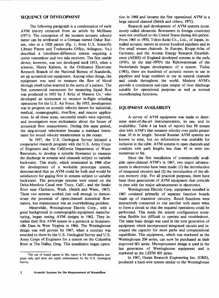
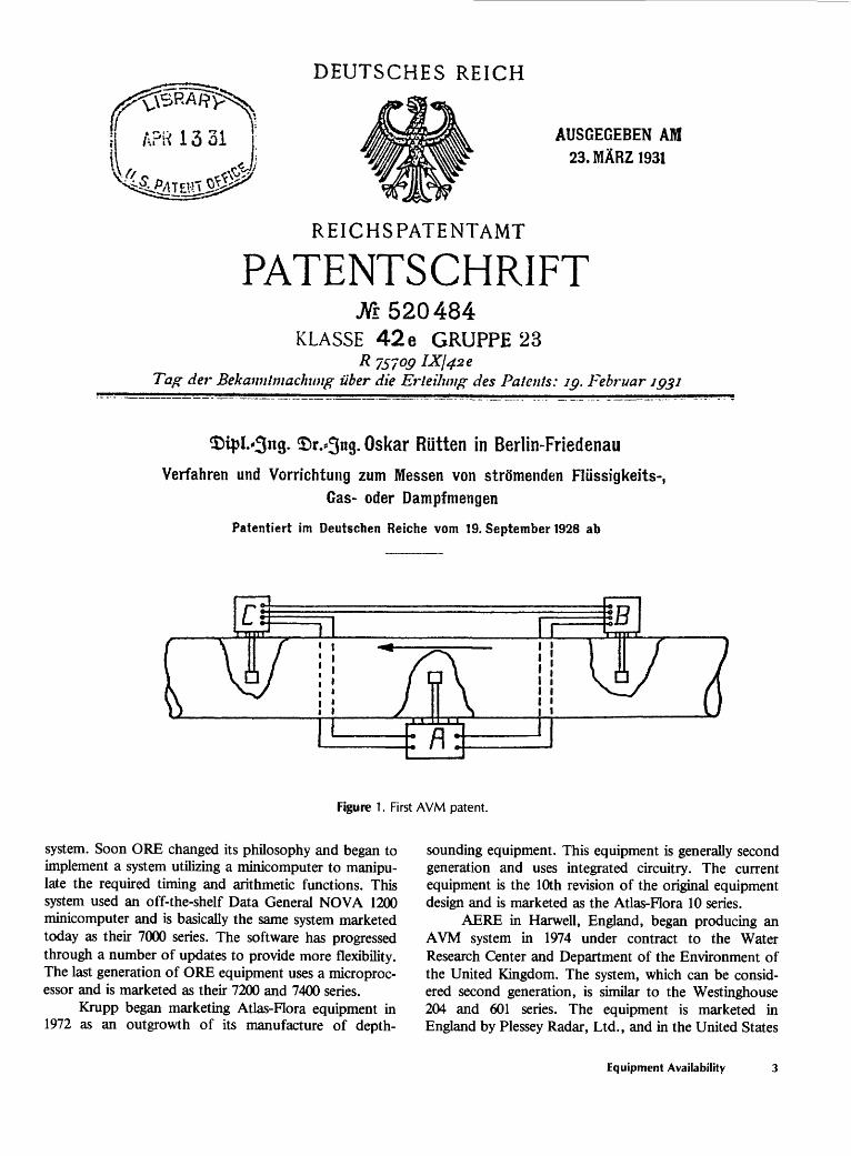
SEQUENCE OF DEVELOPMENT

The following paragraph is a condensation of early AVM history extracted from an article by McShane (1971): The conception of the modern acoustic velocity meter can be attributed to a German named Oskar Rut- ten, who in a 1928 patent (fig. 1, from U.S. Scientific Library Patent and Trademarks Office, Arlington, Va.) described a traveltime-difference system requiring a center transmitter and two side receivers. The first usable device, however, was not developed until 1953, when a scientist, Henry Kalmus, in the Ordinance Electronic Research Branch of the National Bureau of Standards, set up acoustical test equipment. Among other things, the equipment was used to measure the flow of blood through small tubes inserted in the aorta of a patient. The first commercial instrument for measuring liquid flow was produced in 1955 by J. Kritz of Maxson Co. 1 who developed an instrument to monitor in-flight refueling operations for the U.S. Air Force. By 1955, development was in progress on acoustic velocity meters for industrial, medical, oceanographic, riverflow, and reactor applica tions. In all these areas, successful results were reported, and investigators were enthusiastic about the future of acoustical flow measurement. During this same period, the sing-around velocimeter became a standard instru ment for sound velocity measurement in the ocean.

In 1957, the U.S. Geological Survey initiated a cooperative research program with the U.S. Army Corps of Engineers and the California Department of Water Resources, to develop a suitable flowmeter to measure the discharge in streams and channels subject to variable backwater. This study, which terminated in 1966 after the development of a workable prototype system, demonstrated that an AVM could be built and would be satisfactory for gaging flow in streams subject to variable backwater. The prototype systems were tested on the Delta-Mendota Canal near Tracy, Calif., and the Snake River near Clarkston, Wash. (Smith and Wires, 1967). These two systems worked just well enough to demon strate the potential of open-channel acoustical flowmeters, but maintenance was an overwhelming problem.

Meanwhile, Westinghouse Electric Corp., with a good background in oceanographic-equipment manufac turing, began testing AVM designs in 1962. They in stalled their first AVM system in a penstock at Sommers- ville Dam in West Virginia in 1964. The Westinghouse design was well proven by 1967, when a contract was awarded to them by the U.S. Geological Survey and U.S. Army Corps of Engineers for a system on the Columbia River at The Dalles, Oreg. This installation began opera-

The use of brand names in this report is for identification pur poses only and does not imply endorsement by the U.S. Geological Survey.

tion in 1968 and became the first operational AVM in a large natural channel (Smith and others, 1971).

Research and development of AVM systems (com monly called ultrasonic flowmeters in foreign countries) were not confined to the United States during this period. From 1965 to 1970, Tokyo Keiki Co., Ltd., of Japan, in stalled acoustic meters in several hundred pipelines and in five small stream channels. In Europe, Krupp-Atlas of Germany, and the Atomic Energy Research Establish ment (AERE) of England developed systems in the early 1970's. In the mid-1970's the Rijkswaterstaat of the Netherlands began development of a system. Today (1981), there are hundreds of acoustic meters in use in pipelines and large numbers in use in natural channels and canals throughout the world. Modern AVM's provide a continuous real-time output of river discharge suitable for operational purposes as well as normal recordkeeping functions.

EQUIPMENT AVAILABILITY

A survey of AVM equipment was made to deter mine state-of-the-art instrumentation, its use, and its availability. Table 4 (at back of report) lists 88 stream sites with AVM's that measure velocity over paths greater than 10 m in length. Several Russian AVM systems are known to exist, but no information was available for inclusion in the table. AVM systems in open channels and conduits with path lengths less than 10 m were too numerous to list.

Since the first installation of commercially avail able open-channel AVM's in 1967, two major advance ments in electronics have been made: (1) the introduction of integrated circuitry and (2) the introduction of the sili con memory chip. For all practical purposes, there have been three generations of AVM equipment that coincide in time with the major advancements in electronics.

Westinghouse Electric Corp. equipment installed in 1967 consisted primarily of separate function boards made up of transistor circuitry. Board functions were interactively connected to one another with many wires to form a circuit so that the required operations could be performed. This made the system configuration some what flexible but difficult to operate and troubleshoot. The same basic design was used in the next generation of equipment which incorporated integrated circuits and in creased the capacity for more paths and computational capabilities. This equipment, which was marketed as the Westinghouse 204 series, can now be purchased as their improved 601 series. Microprocessor design is used in the last generation of Westinghouse equipment and is marketed as the LEFM 801 series.

In 1967, Ocean Research Engineering Inc. (ORE), produced a hard-wire system similar to the Westinghouse


DEUTSCHES REICH

AUSGEGEBEN AM 23.MARZ1931

REICHSPATENTAMT

PATENTSCHRIFTJVr520484

KLASSE 42 e GRUPPE 2315109

Tag der Bekanntmachung fiber die Erleihtng des Patents: 19. Februar 1931

- Oskar Riitten in Berlin-FriedenauVerfahren und Vorrichtung zum Messen von strdmenden Fliissigkeits-,

Gas- oder Dampfmengen

Patentiert im Deutschen Reiche vom 19. September 1928 ab

/ f 1 *H

Figure 1. First AVM patent.

system. Soon ORE changed its philosophy and began to implement a system utilizing a minicomputer to manipu late the required timing and arithmetic functions. This system used an off-the-shelf Data General NOVA 1200 minicomputer and is basically the same system marketed today as their 7000 series. The software has progressed through a number of updates to provide more flexibility. The last generation of ORE equipment uses a microproc essor and is marketed as their 7200 and 7400 series.

Krupp began marketing Atlas-Flora equipment in 1972 as an outgrowth of its manufacture of depth-

sounding equipment. This equipment is generally second generation and uses integrated circuitry. The current equipment is the 10th revision of the original equipment design and is marketed as the Atlas-Flora 10 series.

AERE in Harwell, England, began producing an AVM system in 1974 under contract to the Water Research Center and Department of the Environment of the United Kingdom. The system, which can be consid ered second generation, is similar to the Westinghouse 204 and 601 series. The equipment is marketed in England by Plessey Radar, Ltd., and in the United States

Equipment Availability

by Redland Automation, Ltd., both under nonexclusive license by Harwell AERE.

Tokyo Keiki Co., Ltd., of Japan, one of the earliest manufacturers of open-channel AVM's, instru mented several sites in 1969. The equipment was mar keted in the United States by Badger Meter Co. Tokyo Keiki has since concentrated on equipment to measure flow in pipes and small channels. These companies are no longer affiliated, and Badger now manufactures a series of pipe and small-channel AVM's of their own design.

Fokker Aircraft Industries, of Amsterdam, manu factures an AVM developed by the Institution of Applied Physics in cooperation with the Hydro-Instrumentation Department of Rijkswaterstaat of the Netherlands. Systems are marketed as the AKWA 76 series, which in cludes the use of a DEC PDP/11/03 minicomputer. The DEC minicomputer performs the same functions as the NOVA minicomputer of the ORE system. The basic dif ference in the systems lies in the acoustic circuitry. A fixed-gain preamplifier and transmitter is built into the Fokker transducer assembly and submerged with it. Other systems do not have preamplifiers or transmitters in their transducers.

Many more manufacturers produce systems that measure velocity and discharge over smaller distances, but they have not been included in this report.

BASIC PRINCIPLES

Two basic methods are used in the acoustic measurement of flow: (1) the time-of-travel method, where sound waves are transmitted along a diagonal in both directions relative to the fluid flow and traveltimes are measured in each direction, and (2) the Doppler shift method, where sound waves are projected along or diag onal to the flow path, and the frequency shift in the return signal (from backscattering of particles in the fluid) is measured.

For streamflow applications, time-of-travel equip ment is more important in terms of basic capabilities and available systems.

Time-of-Travel Method

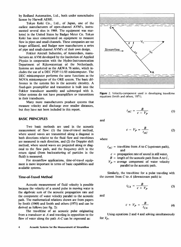
Acoustic measurement of fluid velocity is possible because the velocity of a sound pulse in moving water is the algebraic sum of the acoustic propagation rate and the component of water velocity parallel to the acoustic path. The mathematical relations shown are from papers by Smith (1969) and Smith and others (1971) and can be derived as follows (see fig. 2):

The traveltime of an acoustic pulse originating from a transducer at A and traveling in opposition to the flow of water along the path A-C can be expressed as:

Figure 2. Velocity-component used in developing traveltime equations (Smith and others, 1971).

B1ACC - (1)

and

C ~~" B1AC

(2)

where

tAC = traveltime from A to C (upstream path),and

c = propagation rate of sound in still water, B = length of the acoustic path from A to C,

Vp = average component of water velocity parallel to the acoustic path.

Similarly, the traveltime for a pulse traveling with the current from C to A (downstream path) is:

B1 CA

C +(3)

and

c + Vp = B1 CA

(4)

Using equations 2 and 4 and solving simultaneously for VP ,


2 \tCA 1AC.(5)

and as

then

VP =

B

VL cos e

i2 cos 0 \tCA tAC

(6)

(7)

where

VL = line velocity (the average water velocity at thedepth of the acoustic path), and

6 - angle of departure between the streamline of flow and the acoustic path.

Note that the acoustic propagation rate (c) in equa tions 2 and 4 is canceled in equations 5 and 7 and is not a factor in computing water velocity. This feature makes use of equation 7 in conjunction with time-of-travel equipment valuable in computing water velocity in natural conditions. Fluctuations in the propagation rate owing to changes in water temperature and other density differences have no effect on the computation of water velocity.

Generally, three techniques are now used to deter mine upstream and downstream traveltimes: (1) Travel- time is obtained by directly measuring the time between the initiation of the tra*nsmit pulse and the first cycle of the received pulse, (2) pulse-repetition frequency is ob tained by measuring the frequency of upstream and downstream pulse trains with respect to a given time interval, and (3) phase shift is measured by merging re ceived transmissions of continuous signals. Another tech nique not yet widely used is to correlate the best received signal to the transmitted signal.

DIRECT TRAVELTIME

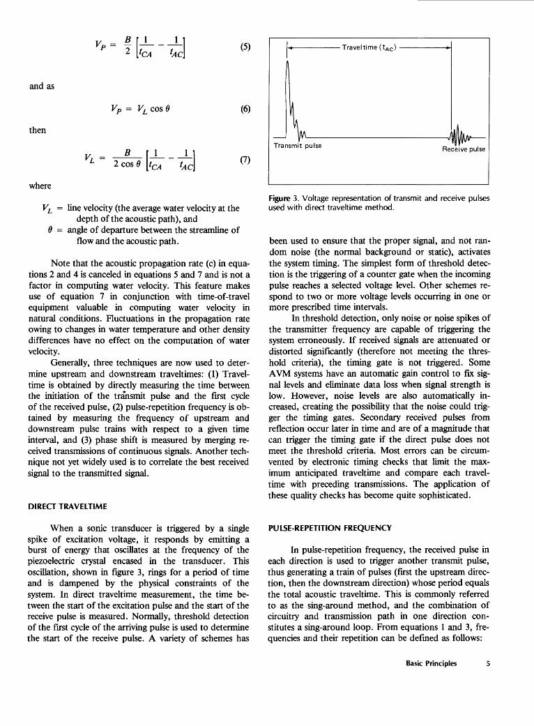
When a sonic transducer is triggered by a single spike of excitation voltage, it responds by emitting a burst of energy that oscillates at the frequency of the piezoelectric crystal encased in the transducer. This oscillation, shown in figure 3, rings for a period of time and is dampened by the physical constraints of the system. In direct traveltime measurement, the time be tween the start of the excitation pulse and the start of the receive pulse is measured. Normally, threshold detection of the first cycle of the arriving pulse is used to determine the start of the receive pulse. A variety of schemes has

Traveltime (tAC )

Transmit pulse Receive pulse

Figure 3. Voltage representation of transmit and receive pulses used with direct traveltime method.

been used to ensure that the proper signal, and not ran dom noise (the normal background or static), activates the system timing. The simplest form of threshold detec tion is the triggering of a counter gate when the incoming pulse reaches a selected voltage level. Other schemes re spond to two or more voltage levels occurring in one or more prescribed time intervals.

In threshold detection, only noise or noise spikes of the transmitter frequency are capable of triggering the system erroneously. If received signals are attenuated or distorted significantly (therefore not meeting the thres hold criteria), the timing gate is not triggered. Some AVM systems have an automatic gain control to fix sig nal levels and eliminate data loss when signal strength is low. However, noise levels are also automatically in creased, creating the possibility that the noise could trig ger the timing gates. Secondary received pulses from reflection occur later in time and are of a magnitude that can trigger the timing gate if the direct pulse does not meet the threshold criteria. Most errors can be circum vented by electronic timing checks that limit the max imum anticipated traveltime and compare each traveltime with preceding transmissions. The application of these quality checks has become quite sophisticated.

PULSE-REPETITION FREQUENCY

In pulse-repetition frequency, the received pulse in each direction is used to trigger another transmit pulse, thus generating a train of pulses (first the upstream direc tion, then the downstream direction) whose period equals the total acoustic traveltime. This is commonly referred to as the sing-around method, and the combination of circuitry and transmission path in one direction con stitutes a sing-around loop. From equations 1 and 3, fre quencies and their repetition can be defined as follows:

Basic Principles

fAC =1AC B (8)

and

1 C+Vr

1CA B (9)

where

fAC = pulse transmission frequency in the downstream direction, and

fCA = pulse transmission frequency in the upstream di rection, then

rf =1 1

1CA 1AC B (10)

where

rf = pulse repetition frequency.

Two drawbacks to this system are (1) the repetition frequency is normally small and the counting interval long, resulting in slow response time for the necessary resolution; and (2) reflected signals from previous transmissions tend to trigger the system at erroneous times. However, these problems have been successfully accommodated, and many AVM systems, particularly those used in pipelines, utilize this concept.

PHASE DETECTION

When sinusoidal signals of a given frequency are transmitted, the phase shift (time shift, not frequency shift) between upstream and downstream signals is

</> = 2/C/C4 ~ 'AC* =C2 - K

(11)

Equation 11 (McShane, 1971) illustrates that the phase difference (</>) can be made larger and easier to measure by increasing the transducer frequency (/), which is generally an advantage.

The speed of sound is determined by measuring tAC and 'C4

2 '*Uc *CA(12)

and is achieved by sensing the start of the transmission

cycle and the start of the reception cycle in both upstream and downstream directions.

Sonic transducers can emit a continuous sinusoidal wave if driven by an oscillator. If two short-duration wave transmissions are emitted in upstream and down stream directions, their resulting received waveforms can be beat (superimposed) with an oscillator waveform whose frequency is near that used to drive the trans mitter. In turn, the resultant waveforms can be super imposed, and the zero crossings will yield the time differential required for line-velocity measurement. The start of the reception cycle is determined by zero-voltage referencing of the modulated receive signal or aperture. Using the entire transmitted signal as a detector makes detection considerably less sensitive to noise but more susceptible to distortion from multipath interference. However, it is physically impractical to operate trans ducers for even short durations with as much voltage as is used by direct traveltime systems, so phase detection systems normally operate with less penetrating power.

CORRELATION COMPARISON

Sonic transducers can be driven to any frequency within a limited range of the resonant frequency of the piezoelectric crystal. Therefore, a sonic transducer is capable of emitting a frequency-modulated signal, and this signal can be modulated to create a pattern or "signature." This pattern can be digitized and placed in computer memory. The receiving transducer is activated at some calculated time after transmit and the reception digitized and stored. Sequential portions of the received data are then compared to the transmitted data by step ping through overlapping blocks of time. The best fit yields a maximum correlation function, and the time of the corresponding step number determines the traveltime. Another method to define a unique transmit pattern is by pulse conditioning techniques which emit a deformed pulse or "chirp."

A similar but simpler method tried by the Dutch (J. G. Drenthen, Rijkswaterstaat, oral commun., 1981) is to digitize time-voltage points of an anticipated receive signal from a single-burst transmission and correlate it with actual received data transmissions. Results show that this technique increases the reliability of attenuated signals but that it does not appreciably increase signal reliability where distortion exists. Correlation schemes are still in the experimental stage but show some promise in situations where appreciable signal attenuation and distortion occur. A modified signal will have the advan tage of being identifiable in the noise level rather than having to exceed the noise level. Little or no filtering will be necessary and the dynamic range of the receiver will be increased.

6 Acoustic Systems for the Measurement of Streamflow

Doppler-Shift Method

Motion of a scattering object will change the fre quency of a returned signal. The frequency of sound observed (scattered) from an object moving in a path directly away from the source is

/o=/5(c-K0)/c (13)

where/0 = the observed frequency,fs = the source frequency,KO = the velocity of the object, andc= the velocity of sound.

From the point of view of a fixed receiver at the source location, the scattering object becomes a moving source and the frequency (fr) at the receiver is

fr=fs (14)

travel equipment because it has greater susceptibility to interference from boundary conditions (bottom and sur face reflections), and is subject to signal attenuation from the same particles necessary in backscattering the signal. In contrast with time-of-travel systems, Doppler systems operate with a larger statistical scatter from individual measurements of shift, and require a great many more samples to obtain reliable results.

LIMITING CRITERIA

Four basic phenomena that affect the performance of acoustical equipment in measuring streams are (1) the multipath phenomenon that is dependent on cross-sec tion geometry, (2) the ray-bending phenomenon caused by temperature or conductivity gradients, (3) the signal- attenuation phenomenon caused by sediment and en trained air, and (4) variable streamline orientation or large eddy flows.

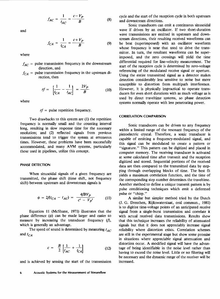
Measurement of the Doppler frequency shift versus time provides a means of determining the velocity of the water mass versus distance along the transducer beam (fig. 4). By assuming that the scatters are moving with the velocity of the water, the frequency data and range is converted to water velocity versus transverse distance across the river. Ranging is done by allowing designated time intervals to listen for backscattering frequencies. Velocity of sound (designated time intervals) is adjusted by a reference backscatter at a known distance.

Doppler equipment can measure stream velocity provided sufficient particles or air bubbles are suspended in the streamflow to backscatter the signal. The lower threshold is not known. Doppler equipment, capable of measuring velocity at remote points using only one trans ducer, can be an excellent system for many applications of fluid-flow measurement. However, the Doppler method lacks the penetration capabilities of time-of-

-DOPPLER SONAR SIGNAL PROCESSOR

Multipath Phenomena

Lowell (1977) has postulated that a reflected signal that arrives at a receiver within one wavelength of the direct signal will cancel the first pulse of the signal (fig. 5). Therefore, this phenomonon is a limiting criterion for locating transducers based on cross-section geometry and the clearance height in figure 5 is the minimum height needed to avoid multipath problems. Table 1 gives some typical statistics for frequencies generally used in streamflow applications.

Accuracy of AVM systems depend on the precision with which the individual traveltimes can be measured. Errors in indicated velocities are a linear function of tim ing error in either direction. Table 1 shows errors that could result if timing in one direction were triggered by the first pulse of the receive signal and timing in the other direction was triggered by the second pulse of the receive

DIAGONAL _PAIHA^OSSJIRE AM

SAMPLE RANGE GATED SEGMENT

Figure 4. Doppler-ranging technique (AMETEK, 1979).

Limiting Criteria

Let

Reflector (bottom or surface)

EXPLANATION'- In this example, it is necessary to determine clearance height in order to locate trans ducers. Signals arriving via any reflected signal path must arrive at least one wavelength later than direct signal.

wavelength frequency velocity of sound path lengthclearance height c F

L + X= 2

since X < L, then X2 ^ 0

and H ~ vS~

Figure 5. Multipath interference (modified from Lowell, 1977).

Table 1. Typical path length versus operating frequency,

clearance height, and effects of one carrier-cycle timing error

[For clearance height, see figure 5]

Path length(meters)

500-1,000200- 50050- 20020- 505- 201- 5

Operatingfrequency

(kHz)

30100200300500

1,000

Clearanceheight

(meters)

3.5 -5.01.2 -1.90.43-0.870.22-0.350.09-0.170.03-0.06

Velocity error for onecarrier-cycle timing error

(meters per second)

0.011-0.0040.136-0.0540.230-0.0900.542-0.1452.67 -0.267

signal, a phenomenon that could occur when signals are drastically attenuated.

Ray-Bending Phenomena

The velocity of sound in water is affected by densi ty changes produced by temperature or salinity gradients. Figure 6 shows how the velocity of sound changes with

10 20 30 40 50 60 70

TEMPERATURE, IN DEGREES CELSIUS

Figure 6. Sonic velocity in water.

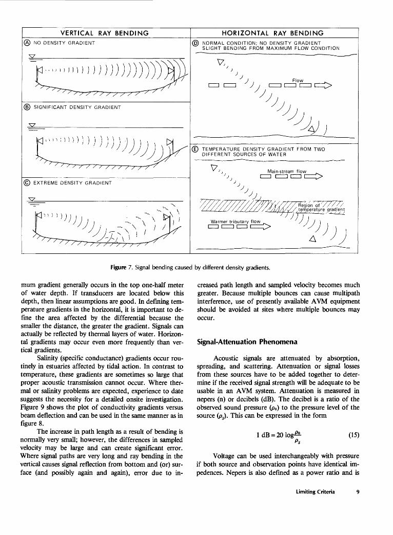
temperature for distilled water and seawater (salinity = 35 g/L). Consequently, ray bending, as illustrated in figure 7, will occur in the presence of either vertical or horizontal density gradients.

Temperature gradients of 0.1 °C per meter or more generally occur in the top one-half meter of a stream cross section in slow moving and ponded water. Below this one-half-meter depth, temperature gradients are nor mally much less than 0.1 °C per meter. Data in an un published report by E. J. Jones (Geological Survey, Sacramento, Calif., Subdistrict) show that out of 183 temperature traverses (24 sites with 15 to 30 observations per site), only five had temperature differences exceeding 0.5°C. Temperature variations at most sites were normal ly too small to measure on the thermistor-type ther mometer that was used. The maximum temperature dif ferential was 4°C, which occurred in summer in a small stream with ponded water. The above data suggest that temperature gradients probably will be of little concern where water is moving, except at sites downstream from tributary flows with a different temperature than that of the main stem or at sites in or near estuaries subject to flow reversal and incomplete mixing with seawater of a different temperature.

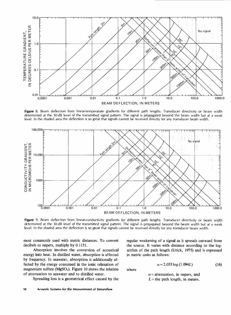
Figure 8 is a plot of beam deflection versus temper ature gradients caused by ray bending based on Snell's law (Clay and Medwin, 1977). For example, if a maxi mum vertical temperature gradient of 0.1 °C per meter can be expected in a stream where a path of 200 m is to be measured, then the maximum signal strength would miss the receiving transducer by 4 m, but a usable signal would be received from the periphery of the 5° cone of trans mission (5° beam width). Given this same temperature gradient and a path of 500 m, the maximum signal strength would be deflected 24 m and no usable signal would be received for a 5° beam width transducer. Tem perature gradients are normally nonlinear and the maxi-


VERTICAL RAY BENDING HORIZONTAL RAY BENDING(A) NO DENSITY GRADIENT

SZ_________________

© NORMAL CONDITION; NO DENSITY GRADIENTSLIGHT BENDING FROM MAXIMUM FLOW CONDITION

Flow C=II=H=>

© SIGNIFICANT DENSITY GRADIENT

[j) TEMPERATURE DENSITY GRADIENT FROM TWO DIFFERENT SOURCES OF WATER

(t) EXTREME DENSITY GRADIENT

Figure 7. Signal bending caused by different density gradients.

mum gradient generally occurs in the top one-half meter of water depth. If transducers are located below this depth, then linear assumptions are good. In defining tem perature gradients in the horizontal, it is important to de fine the area affected by the differential because the smaller the distance, the greater the gradient. Signals can actually be reflected by thermal layers of water. Horizon tal gradients may occur even more frequently than ver tical gradients.

Salinity (specific conductance) gradients occur rou tinely in estuaries affected by tidal action. In contrast to temperature, these gradients are sometimes so large that proper acoustic transmission cannot occur. Where ther mal or salinity problems are expected, experience to date suggests the necessity for a detailed onsite investigation. Figure 9 shows the plot of conductivity gradients versus beam deflection and can be used in the same manner as in figure 8.

The increase in path length as a result of bending is normally very small; however, the differences in sampled velocity may be large and can create significant error. Where signal paths are very long and ray bending in the vertical causes signal reflection from bottom and (or) sur face (and possibly again and again), error due to in

creased path length and sampled velocity becomes much greater. Because multiple bounces can cause multipath interference, use of presently available AVM equipment should be avoided at sites where multiple bounces may occur.

Signal-Attenuation Phenomena

Acoustic signals are attenuated by absorption, spreading, and scattering. Attenuation or signal losses from these sources have to be added together to deter mine if the received signal strength will be adequate to be usable in an AVM system. Attenuation is measured in nepers (n) or decibels (dB). The decibel is a ratio of the observed sound pressure (p0) to the pressure level of the source (ps). This can be expressed in the form

(15)

Voltage can be used interchangeably with pressure if both source and observation points have identical im- pedences. Nepers is also defined as a power ratio and is

Limiting Criteria

10.0 r

0.010.0001 0.001 0.01 0.1 1.0

BEAM DEFLECTION, IN METERS

10.0 100.0 1000.0

Figure 8. Beam deflection from linear-temperature gradients for different path lengths. Transducer directivity or beam width determined at the 30-dB level of the transmitted signal pattern. The signal is propagated beyond the beam width but at a weak level. In the shaded area the deflection is so great that signals cannot be received directly for any transducer beam width.

100,000 rr

L0001 0.001 0.01 0.1 1.0 10.0

BEAM DEFLECTION, IN METERS

100.0 1000.0

Figure 9. Beam deflection from linear-conductivity gradients for different path lengths. Transducer directivity or beam width determined at the 30-dB level of the transmitted signal pattern. The signal is propagated beyond the beam width but at a weak level. In the shaded area the deflection is so great that signals cannot be received directly for any transducer beam width.

most commonly used with metric distances. To convert decibels to nepers, multiply by 0.1151.

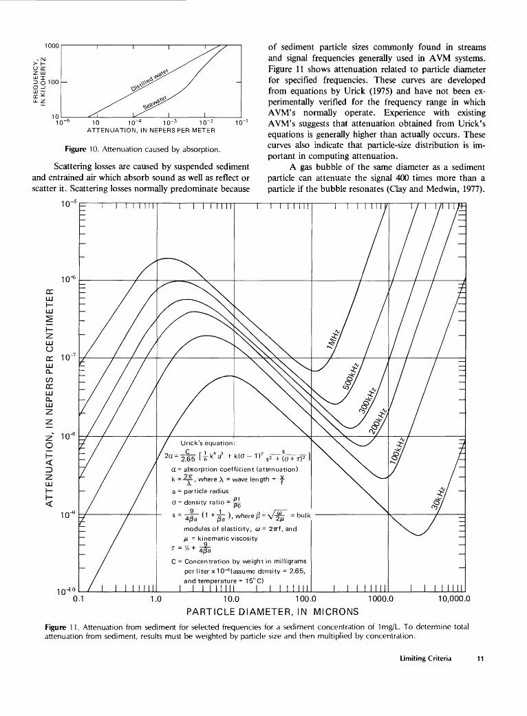
Absorption involves the conversion of acoustical energy into heat. In distilled water, absorption is affected by frequency. In seawater, absorption is additionally af fected by the energy consumed in the ionic relaxation of magnesium sulfate (MgSO4). Figure 10 shows the relation of attenuation to seawater and to distilled water.

Spreading loss is a geometrical effect caused by the

regular weakening of a signal as it spreads outward from the source. It varies with distance according to the log arithm of the path length (Urick, 1975) and is expressed in metric units as follows:

wherea = 2.0331og(1.094L)

a - attenuation, in nepers, and L = the path length, in meters.

(16)


1000

- N>- h-0 CCZ ujUJ ID O 100O -J

1010"& 10 10'4 10~ 3 10~ 2 10-'

ATTENUATION, IN NEPERS PER METER

Figure 10. Attenuation caused by absorption.

Scattering losses are caused by suspended sediment and entrained air which absorb sound as well as reflect or scatter it. Scattering losses normally predominate because

of sediment particle sizes commonly found in streams and signal frequencies generally used in AVM systems. Figure 11 shows attenuation related to particle diameter for specified frequencies. These curves are developed from equations by Urick (1975) and have not been ex perimentally verified for the frequency range in which AVM's normally operate. Experience with existing AVM's suggests that attenuation obtained from Urick's equations is generally higher than actually occurs. These curves also indicate that particle-size distribution is im portant in computing attenuation.

A gas bubble of the same diameter as a sediment particle can attenuate the signal 400 times more than a particle if the bubble resonates (Clay and Medwin, 1977).

1 fl

LLJr- LLJ

r--z.UJ O

CC LLJ CL

CO DC UJ Q_ UJ

Or-

UJr-h-

10"

10'

10'

10-40

2a = 2.65 L 6" K a T MU - " s 2 +(0+T)2

a= absorption coefficient (attenuation)

k = ^Y, where X = wave length = T-

a = particle radius

(7= density ratio = £i9 ( ] r-^

s = ~^o (1 + -5 ), where j3 = v^TT = bul k

modules of elasticity, co = 2irf, and

fj. = kinematic viscosity

C = Concentration by weight in milligrams

per liter x 10~6 (assume density = 2.65,

and temperature = 15°C)I I I I I MM I I I I I I II I III

0.1 1.0 10.0 100.0

PARTICLE DIAMETER, IN MICRONS

1000.0 10,000.0

Figure 11. Attenuation from sediment for selected frequencies for a sediment concentration of 1mg/L To determine total attenuation from sediment, results must be weighted by particle size and then multiplied by concentration.

Limiting Criteria

Resonation occurs when the bubble is approximately the same diameter as the signal wavelength. Little is known about bubble populations in streams; therefore, attenua tion caused by bubbles cannot always be predicted. Ob servations, using portable acoustic equipment below Grand Coulee Dam, showed signal attenuation from en trained air in the channel for distances of 5 to 8 km below the dam. Data were collected when 7,000 mVs was being spilled. Using an estimated 3 m/s mean velocity, the ob servations imply a bubble persistance of 25 to 45 minutes after water was spilled. Onsite measurements of signal at tenuation should be made at critical times at sites where bubbles from air entrainment could cause problems.

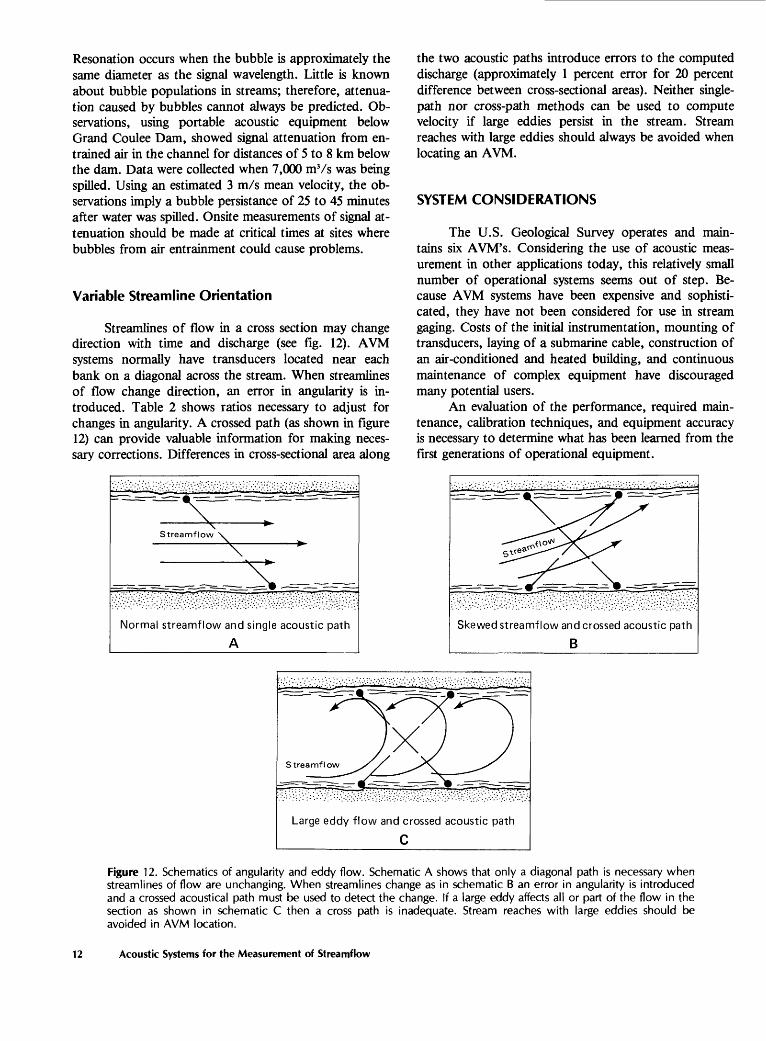
Variable Streamline Orientation

Streamlines of flow in a cross section may change direction with time and discharge (see fig. 12). AVM systems normally have transducers located near each bank on a diagonal across the stream. When streamlines of flow change direction, an error in angularity is in troduced. Table 2 shows ratios necessary to adjust for changes in angularity. A crossed path (as shown in figure 12) can provide valuable information for making neces sary corrections. Differences in cross-sectional area along

Streamflow \\-V >-

Normal streamflow and single acoustic path

the two acoustic paths introduce errors to the computed discharge (approximately 1 percent error for 20 percent difference between cross-sectional areas). Neither single- path nor cross-path methods can be used to compute velocity if large eddies persist in the stream. Stream reaches with large eddies should always be avoided when locating an AVM.

SYSTEM CONSIDERATIONS

The U.S. Geological Survey operates and main tains six AVM's. Considering the use of acoustic meas urement in other applications today, this relatively small number of operational systems seems out of step. Be cause AVM systems have been expensive and sophisti cated, they have not been considered for use in stream gaging. Costs of the initial instrumentation, mounting of transducers, laying of a submarine cable, construction of an air-conditioned and heated building, and continuous maintenance of complex equipment have discouraged many potential users.

An evaluation of the performance, required main tenance, calibration techniques, and equipment accuracy is necessary to determine what has been learned from the first generations of operational equipment.

Skewed streamflow and crossed acoustic path

B

Large eddy flow and crossed acoustic path

Figure 12. Schematics of angularity and eddy flow. Schematic A shows that only a diagonal path is necessary when streamlines of flow are unchanging. When streamlines change as in schematic B an error in angularity is introduced and a crossed acoustical path must be used to detect the change. If a large eddy affects all or part of the flow in the section as shown in schematic C then a cross path is inadequate. Stream reaches with large eddies should be avoided in AVM location.


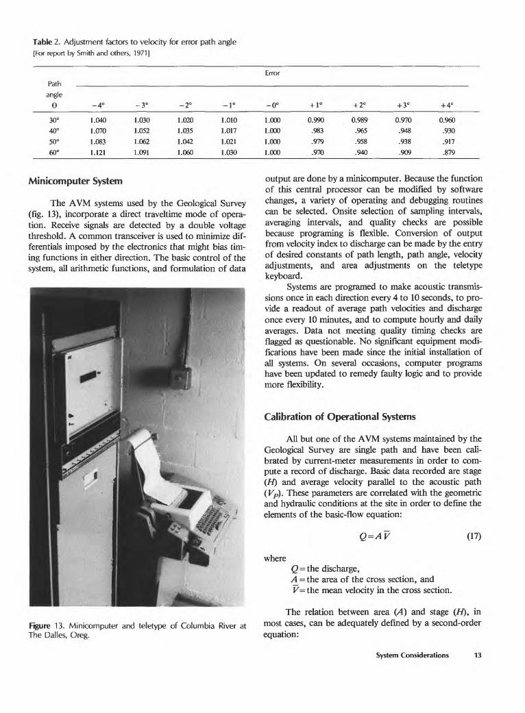
Table 2. Adjustment factors to velocity for error path angle

[For report by Smith and others, 1971]

Pathangle

e30°40°50°60°

-4°

1.0401.0701.0831.121

-3°

1.0301.0521.0621.091

-2°

1.0201.0351.0421.060

-1°

1.0101.0171.0211.030

Error

-0°

1.0001.0001.0001.000

+ 1°

0.990.983.979.970

+ 2°

0.989.965.958.940

+ 3°

0.970.948.938.909

+ 4°

0.960.930.917.879

Minicomputer System

The AVM systems used by the Geological Survey (fig. 13), incorporate a direct traveltime mode of opera tion. Receive signals are detected by a double voltage threshold. A common transceiver is used to minimize dif ferentials imposed by the electronics that might bias tim ing functions in either direction. The basic control of the system, all arithmetic functions, and formulation of data

output are done by a minicomputer. Because the function of this central processor can be modified by software changes, a variety of operating and debugging routines can be selected. Onsite selection of sampling intervals, averaging intervals, and quality checks are possible because programing is flexible. Conversion of output from velocity index to discharge can be made by the entry of desired constants of path length, path angle, velocity adjustments, and area adjustments on the teletype keyboard.

Systems are programed to make acoustic transmis sions once in each direction every 4 to 10 seconds, to pro vide a readout of average path velocities and discharge once every 10 minutes, and to compute hourly and daily averages. Data not meeting quality timing checks are flagged as questionable. No significant equipment modi fications have been made since the initial installation of all systems. On several occasions, computer programs have been updated to remedy faulty logic and to provide more flexibility.

Calibration of Operational Systems

All but one of the AVM systems maintained by the Geological Survey are single path and have been cali brated by current-meter measurements in order to com pute a record of discharge. Basic data recorded are stage (H) and average velocity parallel to the acoustic path (Kp). These parameters are correlated with the geometric and hydraulic conditions at the site in order to define the elements of the basic-flow equation:

Q=AV (17)

where

Figure 13. Minicomputer and teletype of Columbia River at The Dalles, Oreg.

Q=the discharge,A_ =the area of the cross section, and V= the mean velocity in the cross section.

The relation between area (;4) and stage (H), in most cases, can be adequately defined by a second-order equation:

System Considerations 13

(18)

whereCi,C2 , andC3 = constants that can be evaluated from

data obtained during conventional current-meter measurements.

The relation between the path velocity (Vp) and the mean velocity in the cross section can also be represented by a second-order equation:

27

r v K= =y P

(19)

whereK- a ratio (that may or may not include

the path angle), and

C4 , C5 , and C6 = constants evaluated from current-meter measurements and corresponding AVM path velocities.

Substitution of equations 18 and 19 into equation17 results in the general equation:

Q = (C, + C2H+ C3ff) (C4 (20)

Equation 20 can be combined further into a fourth- order equation with five constants, which is done in some programs utilized by USGS systems, but the concepts of rating analysis are simplified if this equation is left in the form shown. This permits separate analysis of area ver sus stage and K versus stage relations.

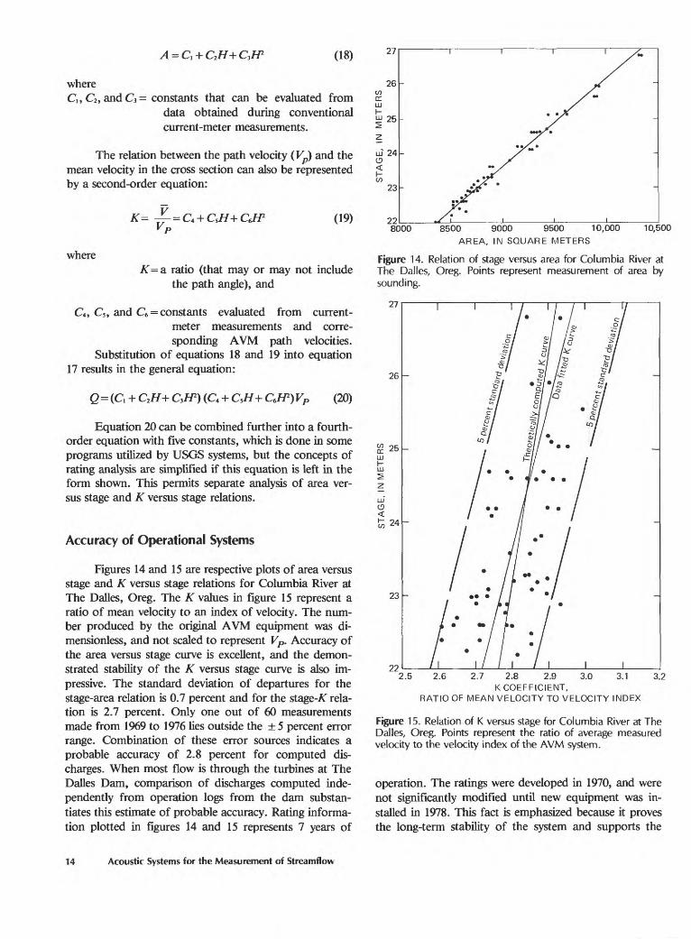
Accuracy of Operational Systems

Figures 14 and 15 are respective plots of area versus stage and K versus stage relations for Columbia River at The Dalles, Oreg. The K values in figure 15 represent a ratio of mean velocity to an index of velocity. The num ber produced by the original AVM equipment was di- mensionless, and not scaled to represent Vp. Accuracy of the area versus stage curve is excellent, and the demon strated stability of the K versus stage curve is also im pressive. The standard deviation of departures for the stage-area relation is 0.7 percent and for the staged rela tion is 2.7 percent. Only one out of 60 measurements made from 1969 to 1976 lies outside the ± 5 percent error range. Combination of these error sources indicates a probable accuracy of 2.8 percent for computed dis charges. When most flow is through the turbines at The Dalles Dam, comparison of discharges computed inde pendently from operation logs from the dam substan tiates this estimate of probable accuracy. Rating informa tion plotted in figures 14 and 15 represents 7 years of

26

25

uI 24U

23

228000 8500 9000 9500 10,000

AREA, IN SQUARE METERS

10,500

Figure 14. Relation of stage versus area for Columbia River at The Dalles, Oreg. Points represent measurement of area by sounding.

27

26

25

24

23

222.5 2.6 3.12.7 2.8 2.9 3.0

K COEFFICIENT, RATIO OF MEAN VELOCITY TO VELOCITY INDEX

3.2

Figure 15. Relation of K versus stage for Columbia River at The Dalles, Oreg. Points represent the ratio of average measured velocity to the velocity index of the AVM system.

operation. The ratings were developed in 1970, and were not significantly modified until new equipment was in stalled in 1978. This fact is emphasized because it proves the long-term stability of the system and supports the


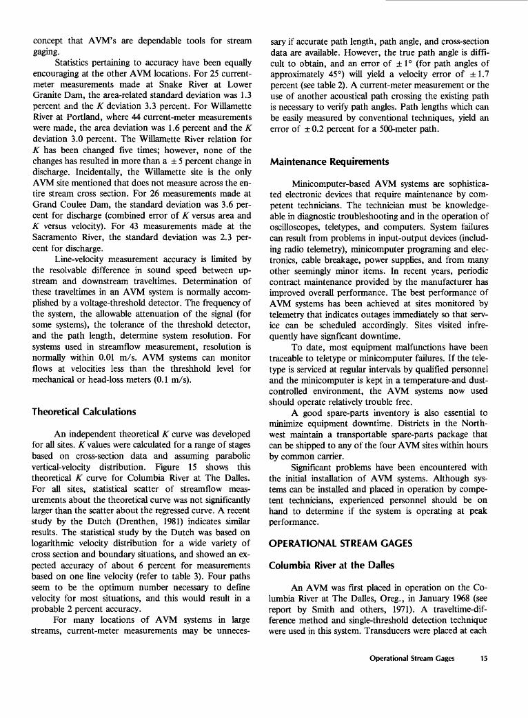
concept that AVM's are dependable tools for stream gaging.

Statistics pertaining to accuracy have been equally encouraging at the other AVM locations. For 25 current- meter measurements made at Snake River at Lower Granite Dam, the area-related standard deviation was 1.3 percent and the K deviation 3.3 percent. For Willamette River at Portland, where 44 current-meter measurements were made, the area deviation was 1.6 percent and the K deviation 3.0 percent. The Willamette River relation for K has been changed five times; however, none of the changes has resulted in more than a ± 5 percent change in discharge. Incidentally, the Willamette site is the only AVM site mentioned that does not measure across the en tire stream cross section. For 26 measurements made at Grand Coulee Dam, the standard deviation was 3.6 per cent for discharge (combined error of K versus area and K versus velocity). For 43 measurements made at the Sacramento River, the standard deviation was 2.3 per cent for discharge.

Line-velocity measurement accuracy is limited by the resolvable difference in sound speed between up stream and downstream traveltimes. Determination of these traveltimes in an AVM system is normally accom plished by a voltage-threshold detector. The frequency of the system, the allowable attenuation of the signal (for some systems), the tolerance of the threshold detector, and the path length, determine system resolution. For systems used in streamflow measurement, resolution is normally within 0.01 m/s. AVM systems can monitor flows at velocities less than the threshhold level for mechanical or head-loss meters (0.1 m/s).

Theoretical Calculations

An independent theoretical K curve was developed for all sites. K values were calculated for a range of stages based on cross-section data and assuming parabolic vertical-velocity distribution. Figure 15 shows this theoretical K curve for Columbia River at The Dalles. For all sites, statistical scatter of streamflow meas urements about the theoretical curve was not significantly larger than the scatter about the regressed curve. A recent study by the Dutch (Drenthen, 1981) indicates similar results. The statistical study by the Dutch was based on logarithmic velocity distribution for a wide variety of cross section and boundary situations, and showed an ex pected accuracy of about 6 percent for measurements based on one line velocity (refer to table 3). Four paths seem to be the optimum number necessary to define velocity for most situations, and this would result in a probable 2 percent accuracy.

For many locations of AVM systems in large streams, current-meter measurements may be unneces

sary if accurate path length, path angle, and cross-section data are available. However, the true path angle is diffi cult to obtain, and an error of ± 1° (for path angles of approximately 45°) will yield a velocity error of ±1.7 percent (see table 2). A current-meter measurement or the use of another acoustical path crossing the existing path is necessary to verify path angles. Path lengths which can be easily measured by conventional techniques, yield an error of ± 0.2 percent for a 500-meter path.

Maintenance Requirements

Minicomputer-based AVM systems are sophistica ted electronic devices that require maintenance by com petent technicians. The technician must be knowledge able in diagnostic troubleshooting and in the operation of oscilloscopes, teletypes, and computers. System failures can result from problems in input-output devices (includ ing radio telemetry), minicomputer programing and elec tronics, cable breakage, power supplies, and from many other seemingly minor items. In recent years, periodic contract maintenance provided by the manufacturer has improved overall performance. The best performance of AVM systems has been achieved at sites monitored by telemetry that indicates outages immediately so that serv ice can be scheduled accordingly. Sites visited infre quently have signficant downtime.

To date, most equipment malfunctions have been traceable to teletype or minicomputer failures. If the tele type is serviced at regular intervals by qualified personnel and the minicomputer is kept in a temperature-and dust- controlled environment, the AVM systems now used should operate relatively trouble free.

A good spare-parts inventory is also essential to minimize equipment downtime. Districts in the North west maintain a transportable spare-parts package that can be shipped to any of the four AVM sites within hours by common carrier.

Significant problems have been encountered with the initial installation of AVM systems. Although sys tems can be installed and placed in operation by compe tent technicians, experienced personnel should be on hand to determine if the system is operating at peak performance.

OPERATIONAL STREAM GAGES

Columbia River at the Dalles

An AVM was first placed in operation on the Co lumbia River at The Dalles, Oreg., in January 1968 (see report by Smith and others, 1971). A traveltime-difference method and single-threshold detection technique were used in this system. Transducers were placed at each

Operational Stream Gages 15

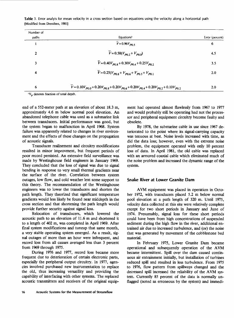
Table 3. Error analyis for mean velocity in a cross section based on equations using the velocity along a horizontal path [Modified from Drenthen, 1981]

Number of paths

1

2

3

4

Equations1

K= 0.50(^.2+^8)

K= 0.40 Kpo.g + 0.30 Fpo.4 + 0.25 Kpo.2

~V 0 25C K -t- V 4- V 4- V V - \).Z3\ VpQ 8 + ^po_6 -l- ^po.3^ KP0.1

Error (percent)

6

4.5

3.5

2.0

2.0

'Vp denotes fraction of total depth.

end of a 552-meter path at an elevation of about 18.3 m, approximately 4.6 m below normal pool elevation. An abandoned telephone cable was used as a submarine link between transducers. Initial performance was good, but the system began to malfunction in April 1968. System failure was apparently related to changes in river environ ment and the effects of these changes on the propagation of acoustic signals.

Transducer realinement and circuitry modifications resulted in minor improvment, but frequent periods of poor record persisted. An extensive field surveillance was made by Westinghouse field engineers in January 1969. They concluded that the loss of signal was due to signal bending in response to very small thermal gradients near the surface of the river. Correlation between system outages, low flow, and cold weather lent some support to this theory. The recommendation of the Westinghouse engineers was to lower the transducers and shorten the path length. They theorized that significant temperature gradients would less likely be found near middepth in the cross section and that shortening the path length would provide further security against signal loss.

Relocation of transducers, which lowered the acoustic path to an elevation of 11.6 m and shortened it to a length of 402 m, was completed in April 1969. After final system modifications and tuneup that same month, a very stable operating system emerged. As a result, sig nal outages of more than an hour were infrequent, and record loss from all causes averaged less than 3 percent from 1969 through 1975.

During 1976 and 1977, record loss became more frequent due to deterioration of certain electronic parts, especially the peripheral output circuitry. In 1977, agen cies involved purchased new instrumentation to replace the old, thus increasing versatility and providing the capability of interfacing with other systems. The replaced acoustic transmitters and receivers of the original equip

ment had operated almost flawlessly from 1967 to 1977 and would probably still be operating had not the proces sor and peripheral equipment circuitry become faulty and obsolete.

By 1978, the submarine cable in use since 1967 de teriorated to the point where its signal-carrying capacity was tenuous at best. Noise levels increased with time, as did the data loss; however, even with the extreme noise problem, the equipment operated with only 10 percent loss of data. In April 1981, the old cable was replaced with an armored coaxial cable which eliminated much of the noise problem and increased the dynamic range of the system.

Snake River at Lower Granite Dam

AVM equipment was placed in operation in Octo ber 1972, with transducers placed 5.2 m below normal pool elevation at a path length of 320 m. Until 1975, velocity data collected at this site were relatively complete except for two short periods in January and June of 1974. Presumably, signal loss for these short periods could have been from high concentrations of suspended sediment during the high flow in the river, additional en trained air due to increased turbulence, and (or) the noise that was generated by movement of the cobblestone bed material.

In February 1975, Lower Granite Dam became operational and subsequently operation of the AVM became intermittent. Spill over the dam caused contin uous air entrainment initially, but installation of turbines reduced spill and resulted in less turbulence. From 1975 to 1976, flow pattern from spillways changed and the decreased spill increased the reliability of the AVM sys tem. Currently 85 percent of the data is normally unflagged (noted as erroneous by the system) and immedi-


ately acceptable when electronic circuitry is functioning. However, the equipment has had about 30 percent downtime because of electronic malfunctions in power supplies, computer circuitry, and teletype components.

Columbia River Below Grand Coulee Dam

AVM equipment was placed in operation in Octo ber 1972, with transducers placed 5.8 m below normal pool elevation and with a path length of 205 m. This system produces a 10-minute average of reservoir out flow that assists the U.S. Bureau of Reclamation with operational control of Grand Coulee Dam.

Initially AVM operation was sporadic. The AVM was placed 1.4 km downstream from the dam to provide a real-time operating record that would be little affected by in-channel storage. The system operated only during those periods when all, or nearly all, the flow passed through the powerplant. Large quantities of air were en trained in the water during periods of spill, causing the attenuation of acoustic signals and loss of data.

Acoustic-transmission problems associated with water turbulence and air entrainment were alleviated by the increased use of the third powerplant which began partial operation in September 1975. For the years 1976, 1977, and 1978, the appraisal of AVM operation indi cated that 75, 84, and 94 percent of the data, respectively, was unflagged and immediately acceptable. The increase in acceptable data correlates with the addition of each new turbine put in operation.

The instrumentation has had its share of electronic malfunctions. Earth-moving activities and heavy con struction nearby caused a very dusty environment inside the instrument shelter. When construction activities ceased, so did most of the electronic problems. Excellent cooperation and assistance from U.S. Bureau of Recla mation personnel, who are in the vicinity at all times, have been helpful in maintaining a high level of perform ance and minimal downtime for this equipment.

Willamette River at Portland

AVM equipment was placed in operation Novem ber 1972, and is in one of the towers of the Morrison Street Bridge. Transducers were placed at an elevation of 3.9 m below mean low water. One transducer was located on the pier of the bridge drawspan and the other on the seawall next to the bridge. The path length of 226 m is about two-thirds of the total channel width. During low- flow periods there is reverse flow from tidal fluctuations.

When this system is in operation, approximately 95 percent of the data is unflagged and immediately accept able; however, there has been considerable downtime be

cause of ships docked in the acoustic path. In 1977, a ship damaged one of the transducers by knocking it from its mount. In February 1978, this problem was resolved by lowering the seawall transducer 2.4 m and protecting it with a shield directly above the mounting.

The submarine cable link used for the Willamette River system is very noisy but adequate for high-quality system performance. The control cable used for electro mechanical functions of the bridge carries the transmit and receive signals on a previously unused pair of con ductors. Other conductors used in this cable carry 60-cycle AC and motor-control signals that induce noise in the pair of conductors used to carry AVM signals. For tunately, no signals are present with frequency characteristics similar to operating frequency of the AVM system.

Sacramento River at Freeport

AVM equipment was placed in operation Novem ber 1978, with transducers placed 2.93 m below summer pool elevation and a path length of 1% m. The AVM produces an hourly average of discharge that assists the county of Sacramento in controlling effluent from the regional waste-water treatment plant. The plant outfall is appromately 79 m downstream from the midpoint of the transducer cross section. A high degree of accuracy and dependability of flow measurement must be maintained, especially during periods of low flow.

Performance of this system has been excellent, with only 10 percent data loss from November 1978 to Octo ber 1980. Most record loss was caused by electrical noise. A nearby faulty powerline insulator seemed to have been the cause of this noise, and therefore has been replaced. During the problem period, the receiver gain had been set lower than normal to keep noise below detector threshold levels.

The calibration of this system has been extremely stable, as evidenced by the fact that a single rating fits all 43 measurements made to within -1-2.5 to -8.8 percent, with a standard departure of 2.3 percent.

Osage River Below Truman Dam

AVM equipment was placed in operation in May 1978, with six transducer paths. The transducer pairs are set 1.5, 3.0, 4.2, 6.0, 7.6, and 8.5 m below mean low water. The streambed is at an average elevation of 9.4 m below mean low water. Path lengths range from 200 to 284 m. The system will provide a record to assist the Army Corps of Engineers with the operational control of Truman Dam. The installation is 600 m downstream from the dam.

Operational Stream Gages 17

To date, performance of the AVM at this site has been very poor. Significant loss of record is attributed to the flow characteristics of the channel and the presence of bubbles in the water. Construction at Truman Dam has not yet been completed, and all water flowing past the AVM has passed over the spillway, entering the channel at an angle and on one side of the stream. Large eddies are produced just below the dam and pass through the measuring section, causing the streamlines to cross the acoustic path at variable angles. Consequently, the AVM can register apparent flows that range from -85 to 285 mVs for constant downstream flow of 140 mVs. None of the acoustic paths in use is a cross-path; however, be cause of the very unstable hydraulic conditions, there is no reason to assume that the errors are random and compensating.

In addition to the undefined-streamline orientation problem, gas bubbles attenuate the acoustic signals below threshold levels. The bubble source is from the produc tion of methane gas by large amounts of decaying organic matter recently submerged during filling of the reservoir.

In addition to the problems above, much damage to the electronic system has been caused by lightning, faulty wiring in the shelter, extremely high-supply voltages, and rats and mice gnawing transducer cables. All the electrical problems have now been resolved. When the hydraulic conditions in the channel are cor rected and the powerhouse goes on line in the fall of 1981, it is anticipated that usable real-time data will be obtained.

Operational Gages in the United Kingdom

Nineteen AVM systems are presently in operation in the United Kingdom (Childs, 1980). Locations of these systems can be found in table 4 (at the back of this report). Two of the systems are multipath and one is a portable system. With satisfactory conditions and effi cient operation, the English single-path systems yield a ±5 percent accuracy. Systems with at least four paths have shown accuracies within ± 1 percent.

Problems regarding AVM operation in the United Kingdom have been varied and numerous; however, the ultrasonic circuitry by itself has been relatively trouble free. The more serious and frequent faults have generally occurred with the peripheral equipment such as paper- tape punches, the depth gage and interface, and the transmitter-receiver switching circuitry. Record loss has also occurred because of changes in the acoustic environ ment. Extreme temperature gradients and heavy weed growth have perpetuated signal loss at a number of in stallations. Attempts to discourage weed growth by lining the channel with a polythene cover have been moderately successful.

Velocity and stage data from the English AVM in stallations are processed in a main-frame computer by their Water Data Unit. Because punch-tape recorders generally operated poorly, processing data was lengthy, and considerable data were lost or unusable.

The English recognize that hydrological instrumen tation and data aquisition systems have and will become more sophisticated, and it is necessary to augment their electronic expertise and develop sound programed main tenance. English maintenance philosophy consists of three basic items, (1) a scheduled maintenance, (2) an adequate technical manual, and (3) a good spare-parts in ventory. They feel it is desirable to have weekly checks by a hydrometric technician and quarterly checks by a quali fied electronics engineer. Adequate documentation is also necessary such that a technician can recognize fault symptoms on site. (Much loss of data in the English AVM systems was perpetuated because an adequate tech nical manual was not available.) Lastly, they feel that a good spare-parts inventory is a necessity but it is very ex pensive. This expense can be held down by using a central holding authority as a means of distribution.

The English feel that site selection is important to AVM operation and that hydraulic, aquatic growth, and temperature-salinity conditions have to be considered. They tend to avoid situations where oblique flow, weeds, and tidal or ponded water could cause potential problems.

RECENT DEVELOPMENTS

Chipps Island Study

The Sacramento River at Chipps Island near Pitts- burg, Calif., has long been a strategic location for measuring the combined outflow of the heavily farmed Sacramento and San Joaquin Valleys. Almost all the outflow is channeled through this relatively narrow tide- affected reach of the river. Operation of the complex California Aqueduct system would be facilitated if a real- time continuous measurement of the net outflow could be achieved at this location. A detailed report by Smith (1969) suggested that a usable measurement of outflow could be made if a suitable AVM system were available.

The Chipps Island channel is about 1,000 m wide with a maximum depth of about 15 m. The path length for an AVM system was about 1,200 m, much of it tra versing a cross section about 9 m in depth. Initially it was thought that a multipath system would provide needed accuracy, but the acoustical environment is complicated by variability in salinity and temperature gradients.

A twice-daily tidal prism moving through the chan nel produces discharges on the order of 8,500 m/s both upstream and downstream. When freshwater outflow is


low, saltwater intrudes up the channel and salt concentra tions on the order of 10,000 to 20,000 mg/L can result. Temperature gradients are also present because of (1) thermal loading from local industries; (2) differences in water temperatures of the Sacramento and San Joaquin River systems, that come together 3 mi to the east; (3) and differences in temperature of the upstream-migrating saline water from San Francisco Bay and the down stream-moving freshwater.

In 1978, transducers, operating at 100, 40, and 24 kHz were installed on the north and south shores of the channel to determine the reliability of acoustical trans missions over a long path in this tidal estuary. Trans missions were activated by a programed transmitter on the north shore and received signals were recorded on the south shore. Tests carried out over a period of about 60 days indicated highly variable attenuation of signal strength. These tests showed more reliable performance at lower frequencies and more consistent acoustic trans missions for paths placed near middepth. Correlations could not be established between performance and any of the parameters of stage, velocity, phases of the tidal cy cle, wind and surface waves, or specific conductance.

A submarine cable was placed across the channel in 1979, and an AVM using 30 kHz transducers was in stalled for evaluation. Analysis of received acoustic signals showed frequent periods when received signals were greatly distorted, causing timing errors of unaccept able magnitude. When signal transmission was poor, the initial part of the received signal was attenuated below the threshold level of the timing circuitry and several cycles of the signal were missed before the timing period terminated. Data-quality checks, built into the AVM computer, could identify gross errors but would not eliminate bias associated with carrier-cycle timing error.

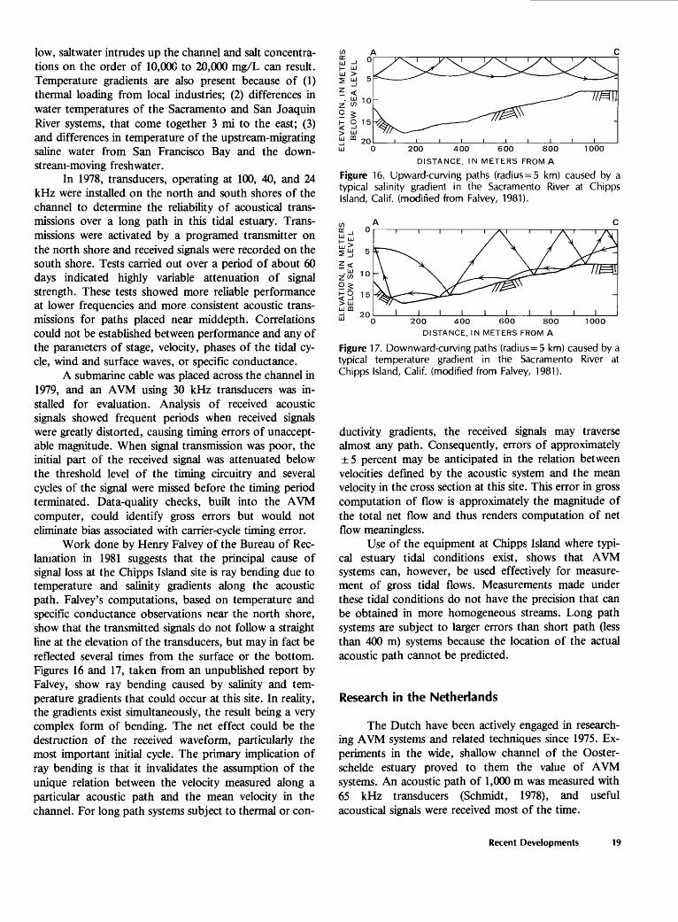
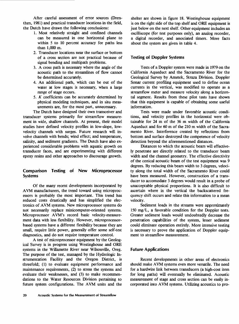
Work done by Henry Falvey of the Bureau of Rec lamation in 1981 suggests that the principal cause of signal loss at the Chipps Island site is ray bending due to temperature and salinity gradients along the acoustic path. Falvey's computations, based on temperature and specific conductance observations near the north shore, show that the transmitted signals do not follow a straight line at the elevation of the transducers, but may in fact be reflected several times from the surface or the bottom. Figures 16 and 17, taken from an unpublished report by Falvey, show ray bending caused by salinity and tem perature gradients that could occur at this site. In reality, the gradients exist simultaneously, the result being a very complex form of bending. The net effect could be the destruction of the received waveform, particularly the most important initial cycle. The primary implication of ray bending is that it invalidates the assumption of the unique relation between the velocity measured along a particular acoustic path and the mean velocity in the channel. For long path systems subject to thermal or con-

H O 15< -l> LiJLJ OQ 20LJ 200 400 600 800 1000

DISTANCE, IN METERS FROM A

Figure 16. Upward-curving paths (radius=5 km) caused by a typical salinity gradient in the Sacramento River at Chipps Island, Calif, (modified from Falvey, 1981).

200 400 600 800

DISTANCE, IN METERS FROM A

1000

Figure 17. Downward-curving paths (radius=5 km) caused by a typical temperature gradient in the Sacramento River at Chipps Island, Calif, (modified from Falvey, 1981).

ductivity gradients, the received signals may traverse almost any path. Consequently, errors of approximately ±5 percent may be anticipated in the relation between velocities defined by the acoustic system and the mean velocity in the cross section at this site. This error in gross computation of flow is approximately the magnitude of the total net flow and thus renders computation of net flow meaningless.

Use of the equipment at Chipps Island where typi cal estuary tidal conditions exist, shows that AVM systems can, however, be used effectively for measure ment of gross tidal flows. Measurements made under these tidal conditions do not have the precision that can be obtained in more homogeneous streams. Long path systems are subject to larger errors than short path (less than 400 m) systems because the location of the actual acoustic path cannot be predicted.

Research in the Netherlands

The Dutch have been actively engaged in research ing AVM systems and related techniques since 1975. Ex periments in the wide, shallow channel of the Ooster- schelde estuary proved to them the value of AVM systems. An acoustic path of 1,000 m was measured with 65 kHz transducers (Schmidt, 1978), and useful acoustical signals were received most of the time.

Recent Developments 19

After careful assessment of error sources (Dren- then, 1981) and practical transducer locations in the field, the Dutch have drawn the following conclusions:

1. Most relatively straight and confined channels can be measured in one horizontal plane to within 5 to 10 percent accuracy for paths less than 1,000 m.

2. Transducer locations near the surface or bottom of a cross section are not practical because of signal bending and multipath problems.

3. A cross path is necessary where the angle of the acoustic path to the streamlines of flow cannot be determined accurately.

4. An additional path, which can be out of the water at low stages is necessary, when a large range of stage occurs.

5. K coefficients can be accurately determined by physical modeling techniques, and in situ meas urements are, for the most part, unnecessary.

The Dutch have designed their own transceiver and transducer systems primarily for streamflow measure ment in wide, shallow channels. At present, their model studies have defined velocity profiles in low-slope, low- velocity channels with surges. Future research will in volve channels with bends; wind effect; and temperature, salinity, and sediment gradients. The Dutch have also ex perienced considerable problems with aquatic growth on transducer faces, and are experimenting with different epoxy resins and other approaches to discourage growth.

Comparison Testing of New Microprocessor Systems

Of the many recent developments incorporated by AVM manufacturers, the trend toward using microproc essors is probably the most important. This trend has reduced costs drastically and has simplified the elec tronics of AVM systems. New microprocessor systems do not necessarily replace minicomputer-oriented systems. Microprocessor AVM's record basic velocity-measure ment data with less flexibility. However, microprocessor- based systems have a different flexibility because they are small, require little power, generally offer some self-test diagnostics, and do not require temperature control.

A test of microprocessor equipment by the Geolog ical Survey is in progress using Westinghouse and ORE systems in the Willamette River near Wilsonville, Oreg. The purpose of the test, managed by the Hydrologic In strumentation Facility and the Oregon District, is threefold; (1) to evaluate equipment performance and maintenance requirements, (2) to stress the systems and evaluate their weaknesses, and (3) to make recommen dations to the Water Resources Division pertaining to future system configurations. The AVM units and the

shelter are shown in figure 18. Westinghouse equipment is on the right side of the top shelf and ORE equipment is just below on the next shelf. Other equipment includes an oscilliscope (for test purposes only), an analog recorder, a digital recorder, and associated timers. More facts about the system are given in table 4.

Testing of Doppier Systems

Tests of a Doppier system were made in 1979 on the California Aqueduct and the Sacramento River for the Geological Survey by Ametek, Straza Division. Doppier Sonar current profiling equipment used to define ocean currents in the vertical, was modified to operate as a streamflow meter and measure velocity along a horizon tal segment. Results from these pilot tests have shown that this equipment is capable of obtaining some useful information.

Tests were made under favorable acoustic condi tions, and velocity profiles in the horizontal were ob tainable for 24 m of the 36 m width of the California Aqueduct and for 60 m of the 210 m width of the Sacra mento River. Interference created by reflections from bottom and surface destroyed the competence of velocity detection beyond the aforementioned distances.

Distances to which the acoustic beam will effective ly penetrate are directly related to the transducer beam width and the channel geometry. The effective directivity of the conical acoustic beam of the test equipment was 9 degrees. By reducing this beam width to 3 degrees, veloci ty along the total width of the Sacramento River could have been measured. However, construction of a trans ducer to accomodate 3 degrees would result in a probe of unacceptable physical proportions. It is also difficult to ascertain where in the vertical the backscattered fre quency shift occurs and relate this information to a mean velocity.

Sediment loads in the streams were approximately 150 mg/L, a favorable condition for the Doppier tests. Greater sediment loads would undoubtedly decrease the penetration capabilities of the system, lesser sediment could eliminate operation entirely. More intensive testing is necessary to prove the application of Doppier equip ment to streamflow measurement.

Future Applications

Recent developments in other areas of electronics should make AVM systems even more versatile. The need for a hardwire link between transducers (a high-cost item for long paths) will eventually be eliminated. Acoustic measurement of stage and cross section can be easily in corporated into AVM systems. Utilizing acoustics to pro-


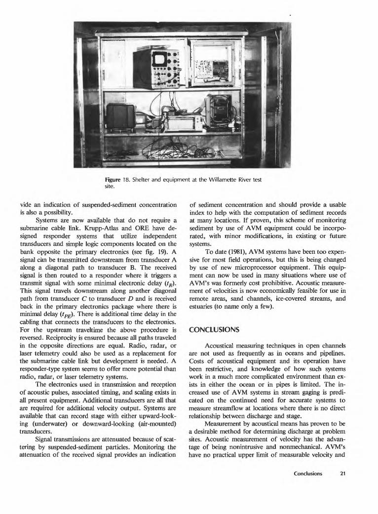
Figure 18. Shelter and equipment at the Willamette River test site.

vide an indication of suspended-sediment concentration is also a possibility.

Systems are now available that do not require a submarine cable link. Krupp-Atlas and ORE have de signed responder systems that utilize independent transducers and simple logic components located on the bank opposite the primary electronics (see fig. 19). A signal can be transmitted downstream from transducer A along a diagonal path to transducer B. The received signal is then routed to a responder where it triggers a transmit signal with some minimal electronic delay (tR). This signal travels downstream along another diagonal path from transducer C to transducer D and is received back in the primary electronics package where there is minimal delay (tPE). There is additional time delay in the cabling that connects the transducers to the electronics. For the upstream traveltime the above procedure is reversed. Reciprocity is ensured because all paths traveled in the opposite directions are equal. Radio, radar, or laser telemetry could also be used as a replacement for the submarine cable link but development is needed. A responder-type system seems to offer more potential than radio, radar, or laser telemetry systems.

The electronics used in transmission and reception of acoustic pulses, associated timing, and scaling exists in all present equipment. Additional transducers are all that are required for additional velocity output. Systems are available that can record stage with either upward-look ing (underwater) or downward-looking (air-mounted) transducers.

Signal transmissions are attenuated because of scat tering by suspended-sediment particles. Monitoring the attenuation of the received signal provides an indication

of sediment concentration and should provide a usable index to help with the computation of sediment records at many locations. If proven, this scheme of monitoring sediment by use of AVM equipment could be incorpo rated, with minor modifications, in existing or future systems.

To date (1981), AVM systems have been too expen sive for most field operations, but this is being changed by use of new microprocessor equipment. This equip ment can now be used in many situations where use of AVM's was formerly cost prohibitive. Acoustic measure ment of velocities is now economically feasible for use in remote areas, sand channels, ice-covered streams, and estuaries (to name only a few).

CONCLUSIONS

Acoustical measuring techniques in open channels are not used as frequently as in oceans and pipelines. Costs of acoustical equipment and its operation have been restrictive, and knowledge of how such systems work in a much more complicated environment than ex ists in either the ocean or in pipes is limited. The in creased use of AVM systems in stream gaging is predi cated on the continued need for accurate systems to measure streamflow at locations where there is no direct relationship between discharge and stage.

Measurement by acoustical means has proven to be a desirable method for determining discharge at problem sites. Acoustic measurement of velocity has the advan tage of being nonintrusive and nonmechanical. AVM's have no practical upper limit of measurable velocity and

Conclusions 21

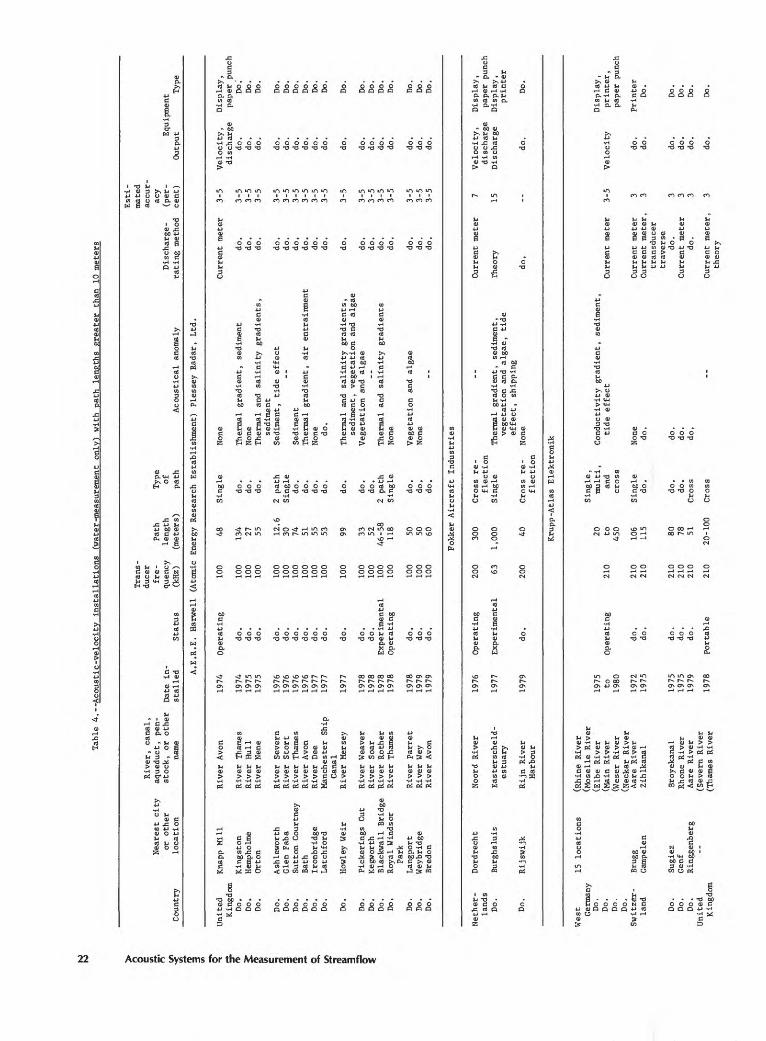
Tabl

e 4.--Ac

oustic-velocity

inst

alla

tion

s (w

ater

-mea

sure

ment

on

ly)

with pa

th le

ngth

s gr

eate

r th

an 10 meters

ftNe

ares

t city

or ot

her

Country

location

United

Knapp

Mill

Kingdom

Do.

Kingston

Do.

Hemp

holm

eDo.

Or ton

Do.

Ashleworth

Do.

Glen F

ab a

Do.

Butt

on C

ourtney

Do .

Bath

Do.

Iron

brid

geDo.

Latc

h ford

Do.

Howley Wei

r

Do.

Pickerings Cut

Do.

Kegw

orth

Do.

Blac

kbal

l Brid

geDo.

Roya

l Wi

ndso

rPa

rkDo

. Langport

Do.

Weyb

ridg

eDo.

Bred

on

Rive

r, ca

nal,

aqueduct,

pen

stoc

k, or

other

name

Rive

r Av

on

Rive

r Thames

Rive

r Hull

River

Nene

River

Severn

River

Stort

River

Thames

Rive

r Av

onRiver

Dee

Manc

hest

er Ship

Cana

lRi

ver

Mers

ey

Rive

r We

aver

River

Soar

Rive

r Ro

ther

Rive

r Th

ames

Rive

r Parr

etRiver We

yRiver

Avon

Date in

stal

led A.

E

1974

1974

1975

1975

1976

1976

1976

1976

1977

1977

1977

1978

1978

1978

1978

1978

1979

1979

Status

.R.E.

Harwell

Oper

atin

g

do.

do.

do.

do.

do.

do.

do.

do.

do.

do.

do.

do.

Experimental

Oper

atin

g

do.

do.

do.

Tran

s

ducer

fre

quen

cy(k

Hz)

(Atomic

100

100

100

100

100

100

100

100

100

100

100

100

100

100

100

100

100

100

Path

length

(meters)

Type of path

Acou

stic

al anomaly

Disc

harg

e-ra

ting

method

Esti

ma

ted

accur

acy

(per

ce

nt)

Equipment

Outp

utType

Ener

gy R

esea

rch

Esta

blis

hmen

t) Pl

esse

y Rada

r, Ltd.

48 134 27 55 12.6

30 74 51 55 53 99 33 5246-58

118 50 50 60

Single

do.

do.

do.

2 path

Sing

ledo.

do.

do.

do.

do.

do.

do.

2 pa

thSi

ngle

do.

do.

do.

None

Ther

mal

grad

ient

, se

dime

ntNo

neTh

erma

l an

d sa

linity gr

adie

nts,

sediment

Sedi

ment

, tide ef

fect

--Sediment

Ther

mal

grad

ient

, ai

r entrainment

None do

.

Ther

mal

and

salini

ty gr

adie

nts,

sedi

ment

, vegeta

tion

and al

gae

Vege

tati

on an

d al

gae

--Thermal

and

salini

ty gradients

None

Vege

tati

on an

d al

gae

None

Current

mete

r

do.

do.

do.

do.

do.

do.

do.

do.

do.

do.

do.

do.

do.

do.

do.

do.

do.

3-5

3-5

3-5

3-5

3-5

3-5

3-5

3-5

3-5

3-5

3-5

3-5

3-5

3-5

3-5

3-5

3-5

3-5

Velo

city

,di

scha

rge

do.

do.

do.

do.

do.

do.

do.

do.

do.

do.

do.

do.

do.

do.

do.

do.

do.

Disp

lay,

paper

punch

DO.'

Do.

Do.

Do.

Do.

Do.

Do.

Do.

Do.

Do.

Do.

Do.

Do.

Do.

Do.

Do.

Do.

Fokk

er A

ircr

aft

Industries

Nether-

Dord

rech

tla

nds

Do.

Burg

hs lui

s

Do.

Rijswijk

Noor

d River

East

ersc

held

-estuary

Rijn

River

Harbour

1976

1977

1979

Oper

atin

g

Experimental

do.

200 63 200

300

1,000 40

Cros

s re

flection

Sing

le

Cros

s re

fl

ecti

on

__

Thermal

gradient,

sediment,

vege

tati

on an

d algae, ti

deef

fect

, sh

ippi

ngNone

Curr

ent meter

Theo

ry

do.

7 15 --

Velocity,

discharge

Disc

harg

e

do.

Disp

lay,

paper

punc

hDi

spla

y,pr

inte

r

Do.

Krup

p-At

las

Elek

tron

ik

West

15 locations

Germany

Do.

Do.

Do.

Do.

Swit

zer-

Brug

gland

Gamp

elen

Do.

Sugiez

Do.

Genf

Do .

Ring

genb

erg

United

Kingdom

(Rhine R

iver

(Mos

elle

River

(Elbe

River

(Mai

n River

(Weser R

iver

(Neckar

River

Aare

Riv

erZi

hlka

nal

Broyekanal

Rhon

e River

Aare

River

(Severn

River

(Tha

mes

Rive

r

1975 to 1980

1972

1975

1975

1975

1979

1978

Oper

atin

g

do.

do.

do.

do.

do.

Portable

210

210

210

210

210

210

210

20 to45

0

106

115 80 78 51

20-100

Sing

le,

mult

i,an

dcross

Sing

ledo.

do.

do.

Cros

s

Cross

Cond

ucti

vity

gra

dient, se

dime

nt,

tide

effect

None do.

do.

do.

do.

"

Curr

ent

mete

r

Current

mete

rCurrent

meter,

tran

sduc

ertr

aver

sedo

.Current meter

do.

Current

meter,

theory

3-5 3 3 3 3 3 3

Velo

city

do.

do.

do.

do.

do.

do.

Display,

prin

ter,

pape

r punch

Prin

ter

Do.

Do.

Do.

Do.

Do.

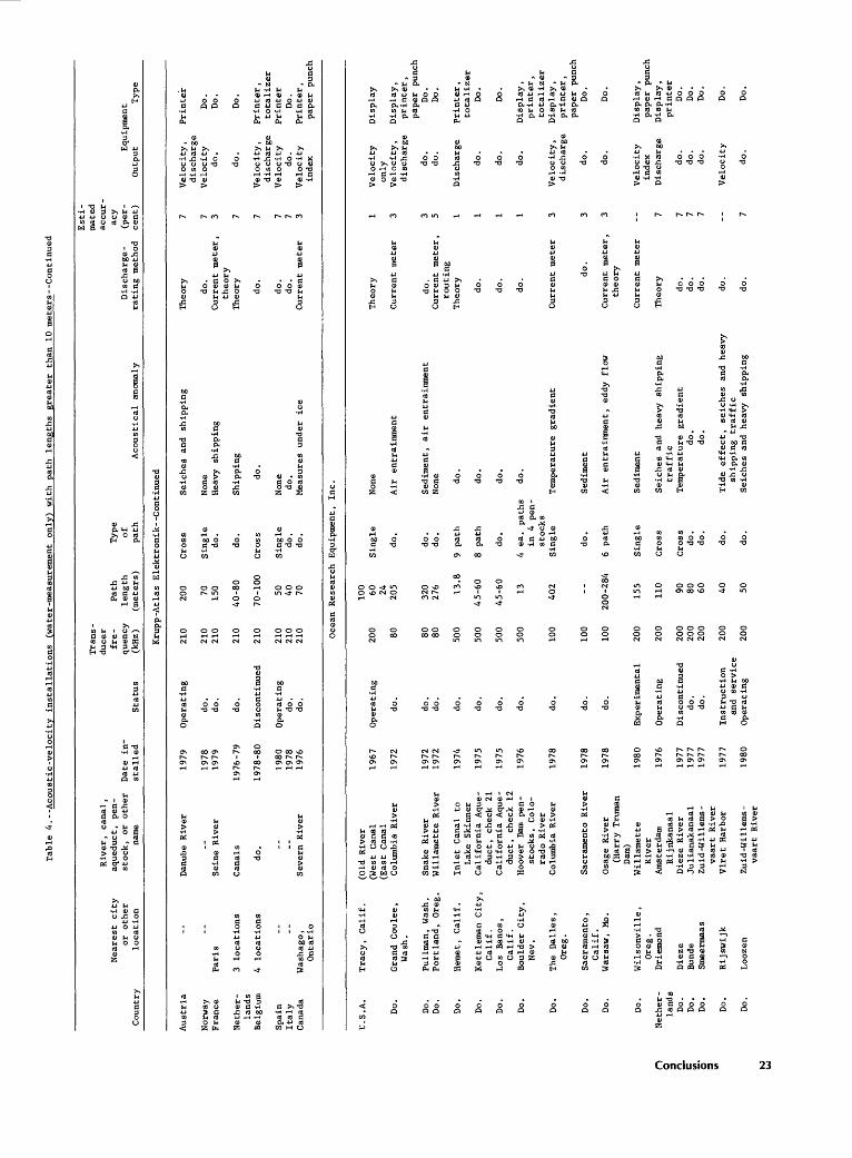
Tabl

e 4.

--Ac

oust

ic-v

eloc

ity

installations

(wat

er-m

easu

reme

nt on

ly)

with path lengths

greater

than 10 meters--Continued

Country

Nearest

city

or ot

her

loca

tion

River, ca

nal,

aqueduct,

pen

stock, or

other

name

Date

in

stal

led

Status

Trans

- du

cer

fre

quen

cy(kHz)

Path

length

(met

ers)

Type of

path

Ac

oust

ical

an

omal

yDi

scha

rge

-ra

ting

method

Esti

mate

d accur

acy

(per

cent)

Equi

pmen

tOutput

Type

Krupp -A

tlas

El

ektr

onik

- -Continued

Aust

ria

Norway

Fran

ce

Neth

er

lands

Belg

ium

Spain

Ital

yCanada

U.S.A. Do.

Do.

Do.

Do.

Do.

Do.

Do.

Do.

Do.

Do.

Do.

O

Nether -

3

lands

Q.

Do.

5

Do.

O*

Do.

3

v>Do.

Do.

.. --Pa

ris

3 locations

4 locations

-- --Wa

shag

o,On

tari

o

Trac

y, Ca

lif.

Grand

Coul

ee,

Wash

.

Pullman, Wash.

Port

land

, Oreg.

Heme

t, Calif.

Kettleman

City,

Calif.

Los

Bano

s,Calif.

Boulder

City,

Nev.

The

Dalles,

Oreg.

Sacramento ,

Cali

f.Wa

rsaw

, Mo

.

Wilsonville,

Oreg

.Dr

iemo

nd

Dieze

Bunde

Smee

rmaa

s

Rijs

wijk

Loozen

Danu

be Ri

ver

--Seine River

Canals do. -- --

Severn R

iver

(Old R

iver

(Wes

t Canal

(Eas

t Ca

nal

Colu

mbia

Riv

er

Snak

e Ri

ver

Willamette Ri

ver

Inle

t Canal

toLake Skinner

Cali

forn

ia Aq

ue

duct

, ch

eck

21Ca

lifo

rnia

Aque

duct,

chec

k 12

Hoov

er Dam

pen

stoc

ks,

Colo

rado

River

Colu

mbia

River

Sacramento River

Osag

e River

(Har

ry Truman

Dam)

Will

amet

teRiver

Amsterdam

Rijnkanaal

Diez

e River

Ju 1 ianakanaa 1

Zuid

-Wil

lems

-vaart

Rive

rVlret

Harbor

Zuid-Willems-

vaar

t Ri

ver

1979

1978

1979

1976-79

1978-80

1980

1978

1976

1967

1972

1972

1972

1974

1975

1975

1976

1978

1978

1978

1980

1976

1977

1977

1977

1977

1980

Oper

atin

g

do.

do.

do.

Discontinued

Oper

atin

gdo.

do.

Oper

atin

g

do.

do.

do.

do.

do.

do.

do.

do.

do.

do.

Experimental

Operating

Disc

onti

nued

do.

do.

Inst

ruct

ion

and

serv

ice

Oper

atin

g

210

210

210

210

210

210

210

210 Ocea

n

200 80 80 80 500

500

500

500

100

100

100

200

200

200

200

200

200

200

200 70 150

40-80

70-1

00

50 40 70

Rese

arch

100 60 24 205

320

276 13.8

45-60

45-60

13

402 --

200-284

155

110 90 80 60 40 50

Cross

Seiches

and

ship

ping

Single

None

do.

Heav

y sh

ippi

ng

do.

Ship

ping

Cros

s do

.

Single

None

do.

do.

do.

Meas

ures

under

ice

Equi

pmen

t , Inc

.

Sing

le

None

do.

Air

entr

ainm

ent

do.

Sediment,

air

entrainment

do .

None

9 pa

th

do.

8 path

do.

do.

do.

4 ea

. paths

do.

in 4

pen

stocks

Single

Temperature

grad

ient

do.

Sediment

6 path

Air

entrainment, ed

dy fl

ow

Single

Sediment

Cross

Seic

hes

and

heav

y sh

ippi

ngtraffic

Cros

s Temperature

gradie

ntdo.

do.

do.

do.

do.

Tide effect,

seiches

and

heav

ysh

ippi

ng tr

affi

cdo.

Seic

hes

and

heavy

ship

ping

Theo

ry do.

Curr

ent

mete

r,th

eory

Theo

ry do.

do.

do.

Current

mete

r

Theo

ry

Current meter

do.

Curr

ent

mete

r,ro

utin

gTheory do.

do.

do.

Curr

ent meter

do.

Current

meter,

theory

Curr

ent

meter

Theo

ry do.

do.

do.

do.

do.

7 7 3 7 7 7 7 3 1 3 3 5 1 1 1 1 3 3 3 -- 7 7 7 7 -- 7

Velocity,

disc

harg

eVe

loci

tydo.

do.

Velocity,

discharge

Velo

city

do.

Velo

city

index

Velo

city

only

Velocity,

disc

harg

e

do.

do.

Disc

harg

e

do.

do.

do.

Velocity,

disc

harg

e

do.

do.

Velo

city

inde

xDi

scha

rge

do.

do.

do.

Velo

city

do.

Prin

ter

Do.

Do.

Do.

Printer,

tota

lize

rPrinter

Do.

Printer,

paper

punch

Disp

lay

Disp

lay,

prin

ter,

pape

r pu

nch

Do.

Do.

Prin

ter,

tota

lize

rDo

.

Do.

Display

,pr

inte

r,to

tali

zer

Disp

lay,

prin

ter,

paper

punc

hDo.

Do.

Disp

lay,

pape

r pu

nch

Display,

prin

ter

Do.

Do.

Do.

Do.

Do.

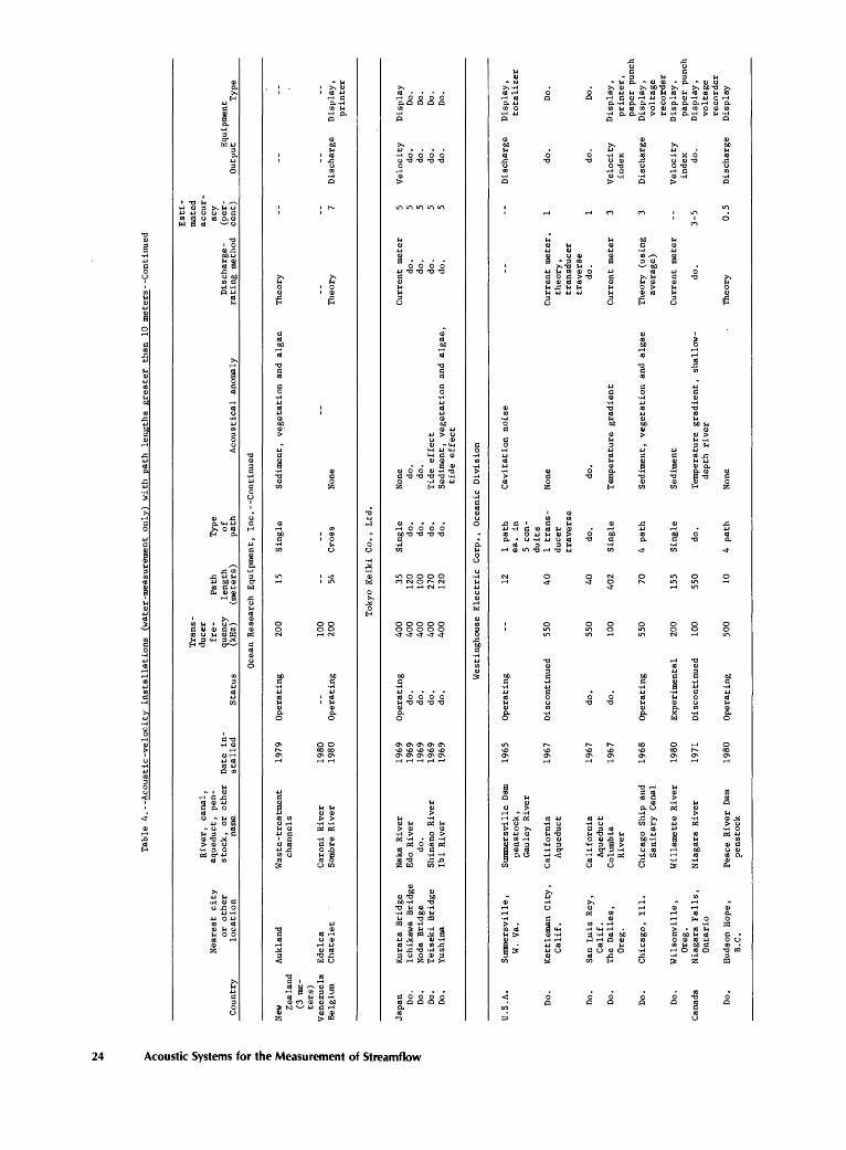
to

u > § a o' (S>

~< V) "*

Country

& $

n ^

New

n

Zealand

|

(3 me-

|

ters

)3

Vene

zuel

an

Belgium

5 0 (S> 3 B» f'

Japan

DO.

*

Do.

Do.

Do.

Tabl

e 4.

--A

cous

tic-

velo

city

in

stal

lati

ons

(wat

er -measurement

only)

with

path le

ngth

s gr

eate

r than 10 met

ers --

Cont

inue

d

Nearest

city

or

other

location

River

, canal

, aq

uedu

ct ,

pen

stoc

k, or

other

name

Date in

stalled

Stat

us

Trans

duce

r fre-

Path

Type

quency

leng

th

of

(kHz

) (m

eter

s)

path

Ocean Re

sear

ch

Aukland

Edel

caCh

atel

et

Kura

ta Br

idge

Ichi

kawa

Br

idge

Noda Br

idge

Teiseki

Brid

geYushima

Waste -treatment

channels

Caro

ni Ri

ver

Sombre Ri

ver

Naka Ri

ver

Edo

Rive

rdo

.Sh

inan

o River

Ibi

Rive

r

1979

1980

1980

1969

1969

1969

1969

1969

Oper

atin

g

--Op

erat

ing

Oper

atin

gdo.

do.

do.

do.

200

100

200

Tokyo

400

400

400

400

400

Acoustical an

omal

y

Esti

mated

accu

r

acy

Disc

harg

e-

(per

- ra

ting

met

hod

cent)

Equipment

Output

Type

Equi

pmen

t, Inc. --Continued

15 -- 54

Sing

le

--Cr

oss

Sedi

ment

, ve

geta

tion

and

alga

e

--None

Theo

ry

..Th

eory

7

-- --Di

scha

rge

-- --Di

spla

y,pr

inte

r

Keiki Co.

, Ltd.

35 120

100

270

120

West

ingh

ouse

El

ectr

ic

U.S.A. Do.

Do.

Do.

Do.

Do.

Canada Do.

Summ

er svi

lie,

W. Va

.

Kettleman

City,

Cali

f.

San

Luis Rey,

Calif.

The

Dalles,

Oreg.

Chic

ago,

11

1.

Wilsonville,

Oreg

.Ni

agar

a Fa

lls,

Ontario

Hudson Hope

,B.

C.

Summersville Dam

penstock,

Gaul

ey R

iver

Cali

forn

iaAqueduct

Cali

forn

iaAqueduct

Colu

mbia

River

Chicago

Ship

and

Sanitary Ca

nal

Will

amet

te Ri

ver

Niag

ara

Rive

r

Peace

Rive

r Da

mpe

nsto

ck

1965

1967

1967

1967

1968

1980

1971

1980

Oper

atin

g

Discontinued

do.

do.

Oper

atin

g

Experimental

Discontinued

Oper

atin

g

..

550

550

100

550

200

100

500

12 40 40 402 70 155

550 10

Single do.

do.

do.

do.

Corp.

, Oc

eani

c

1 pa

thea

. in

5 con

duit

s1 trans

duce

rtr

aver

se

do.

Sing

le

4 pa

th

Sing

le

do.

4 path

None do

.do.

Tide

ef

fect

Sedi

ment

, ve

geta

tion

and algae,

tide effect

Divi

sion

Cavi

tati

on no

ise

None do

.

Temperature

gradient

Sediment,

vege

tati

on and

alga

e

Sediment

Temperature

grad

ient

, shallow-

dept

h river

None

Current

meter

5do.

5do

. 5

do.

5do

. 5

__

Curr

ent meter

, 1

theo

ry,

transducer

traverse

do.

1

Current

meter

3

Theory (using

3av

erag

e)

Current

meter

do.

3-5

Theory

0.5

Velo

city

do.

do.

do.

do.

Disc

harg

e

do.

do.

Velo

city

index

Disc

harg

e

Velocity

inde

x do.

Disc

harg

e

Display

Do.

Do.

Do.

Do.

Display,

tota

lize

r

Do.

Do.

Display,

printer,

pape

r pu

nch

Display,

voltage

reco

rder

Disp

lay,

paper

punch

Display

,vo

ltag

erecorder

Display

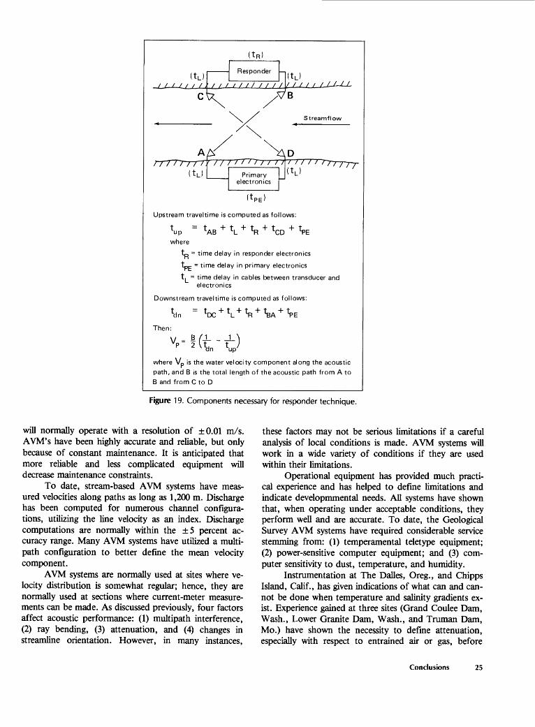
U-

AA'7~7~7~T~

(tj/ /

Primary electronics

J(t L ) ^7~TT

Upstream traveltime is computed as follows:

up

where

= IAB CD

tp = time delay in responder electronics

tpc = time delay in primary electronics

t. = time delay in cables between transducer and electronics

Downstream traveltime is computed as follows:

ldn

- B /!_ _ A.\ 2 ^

Then:

where Vp is the water velocity component along the acoustic

path, and B is the total length of the acoustic path from A to

B and from C to D

Figure 19. Components necessary for responder technique.

will normally operate with a resolution of ±0.01 m/s. AVM's have been highly accurate and reliable, but only because of constant maintenance. It is anticipated that more reliable and less complicated equipment will decrease maintenance constraints.

To date, stream-based AVM systems have meas ured velocities along paths as long as 1,200 m. Discharge has been computed for numerous channel configura tions, utilizing the line velocity as an index. Discharge computations are normally within the ±5 percent ac curacy range. Many AVM systems have utilized a multipath configuration to better define the mean velocity component.

AVM systems are normally used at sites where ve locity distribution is somewhat regular; hence, they are normally used at sections where current-meter measure ments can be made. As discussed previously, four factors affect acoustic performance: (1) multipath interference, (2) ray bending, (3) attenuation, and (4) changes in streamline orientation. However, in many instances,

these factors may not be serious limitations if a careful analysis of local conditions is made. AVM systems will work in a wide variety of conditions if they are used within their limitations.

Operational equipment has provided much practi cal experience and has helped to define limitations and indicate developmmental needs. All systems have shown that, when operating under acceptable conditions, they perform well and are accurate. To date, the Geological Survey AVM systems have required considerable service stemming from: (1) temperamental teletype equipment; (2) power-sensitive computer equipment; and (3) com puter sensitivity to dust, temperature, and humidity.

Instrumentation at The Dalles, Oreg., and Chipps Island, Calif., has given indications of what can and can not be done when temperature and salinity gradients ex ist. Experience gained at three sites (Grand Coulee Dam, Wash., Lower Granite Dam, Wash., and Truman Dam, Mo.) have shown the necessity to define attenuation, especially with respect to entrained air or gas, before

Conclusions 25

locating an AVM system. Problems at the Truman Dam site indicate the necessity of being aware of streamline aberrations before placing transducers. Problems on the Sacramento River site at Freeport have shown the neces sity to investigate electrical noise before specifying system requirements. Increased use of sophisticated electronic AVM systems (as well as other new hydrologic systems) demands more in-house technical expertise.

Past performance has shown that the serviceability pertaining to acoustic circuitry, has been excellent. Hopefully, microprocessor equipment will provide the cost-effective systems long desired and reduce the many logistic and maintenance constraints of the minicomputer systems. New signal-detection techniques and communi cation links may provide additional flexibility so that systems can operate under diverse conditions in rivers and estuaries. Demonstrations are necessary to show the feasibility of using this equipment in situations such as those involving ice-covered streams, sand channels, and estuaries.

SELECTED REFERENCES

American Standards for Tests and Measurements, 1980, Stand ard practice for measurement of water velocity in open channels by acoustic means: American Society of Civil Engineers, Designation D 3857-79, p. 112-118.

AMETEK, 1979, Final report Feasibility demonstration of river current measurement system using Doppler sonar, prepared for the U.S. Geological Survey Contract 14-08-0001-17542: 58 p.

Childs, S. C., 1980, Technical report on ultrasonic gaging in the United Kingdom, Department of the Environment, Water Data Unit Report, 20 p.

Clay, C. S., and Medwin, H., 1977, Acoustical oceanography, Principles and applications: New York, John Wiley, 544 p.

Drenthen, J. G., 1981, The accuracy of the total discharge determined by acoustical velocity measurement: 2nd Sym posium on Flow, Its Measurement and Control in Science and Industry, 20 p.

Lowell, F. C., Jr., 1977, Designing open channel acoustic flowmeters for accuracy, Parts 1 and 2: Water and Sewage Works, July and August issues.

McShane, J. L., 1971, Ultrasonic flowmeters, in Proceedings of the symposium on flow Its measurement and control in science and industry: Pittsburg, Perm., Westinghouse, 20 p.

Schmidt, D., 1978, Acoustic flow measurement in wide rivers: Flow measurement of fluids, Central Organization, TNO, The Hague North-Holland Publishing Co.,391-395 p.

Smith, Winchell, 1969, Feasability study of the use of the acoustic velocity meter for measurement of net outflow from the Sacramento-San Joaquin Delta in California: U.S. Geological Survey Water-Supply Paper 1877, 54 p.

Smith, Winchell, Hubbard, L. L., and Laenen, Antonius, 1971, The acoustic streamflow measuring system on the Colum bia River at The Dalles, Oregon: U.S. Geological Survey open-file report, 60 p.

Smith, Winchell, and Wires, H. O., 1967, The acoustic velocity meter A report on system development and testing: U.S. Geological Survey open-file report, 43 p.

Urick, R. J., 1975, Principles of underwater sound (2nd ed.): New York, McGraw-HUl, 384 p.


U.S. GOVERNMENT PRINTING OFFICE: 1983 676-041/35 REGION NO. 8

Documents

Acoustic Systems for the Measurement of Streamflow - · PDF fileAcoustic Systems for the Measurement of Streamflow By ANTONIUS LAENEN and WINCHELL SMITH U.S. GEOLOGICAL SURVEY WATER-SUPPLY