Embed Size (px)
Citation preview

Acoustic Spectroscopy SimulationAn Exact Solution for Poroelastic Samples
Youli Quan
November 13, 2006
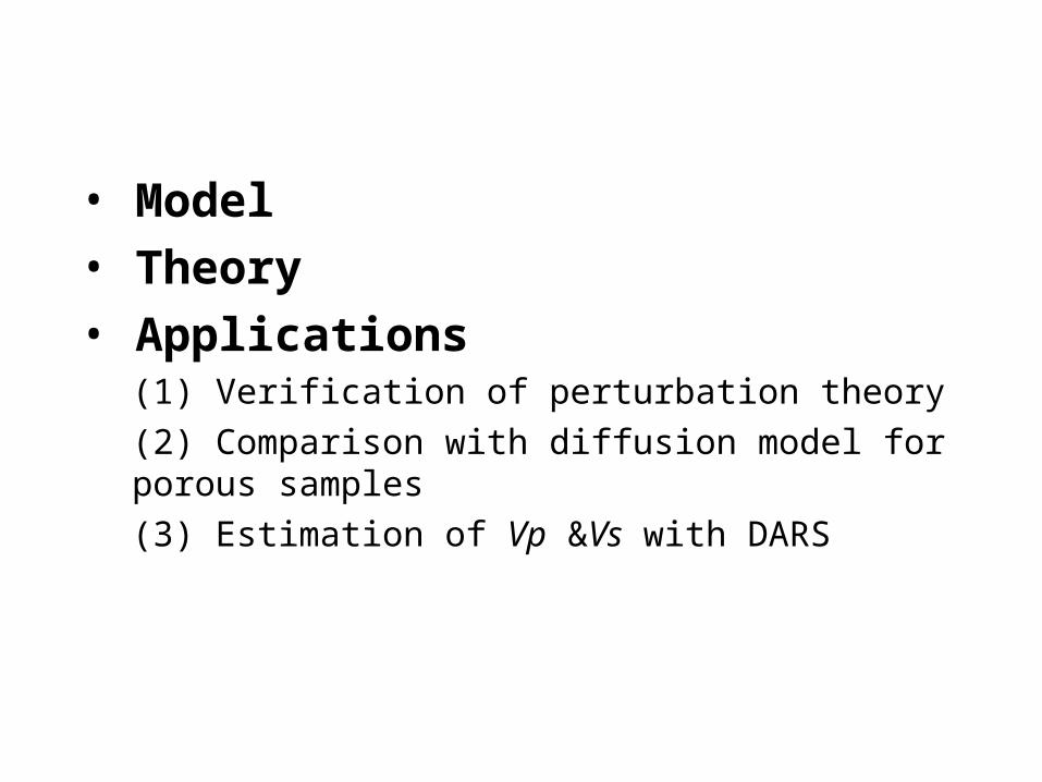
• Model
• Theory
• Applications(1) Verification of perturbation theory
(2) Comparison with diffusion model for porous samples
(3) Estimation of Vp &Vs with DARS
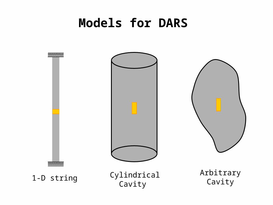
1-D string CylindricalCavity
Arbitrary Cavity
Models for DARS
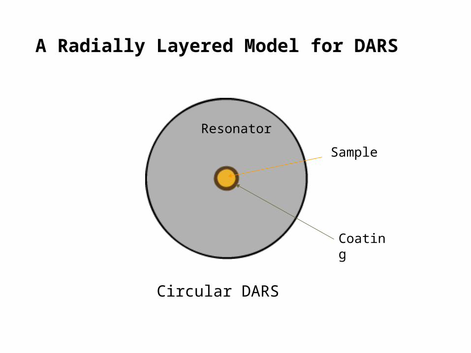
Sample
Coating
Resonator
Circular DARS
A Radially Layered Model for DARS

Generalized Reflection and Transmission Method for Circular DARS
0)~()()(
0)()()()(2
22
wuwu
wuwuu
f
f
MC
CGGH
Governing Equations
H, G, C, M, … are poroelastic parameters

)()()()()( jjjjj cEcEu
Formal Solution in jth layer
Fluid Layer: 2x1 matrices
)( jE
Non-permeable Layer (solid) : 4x2 matrices
Permeable Layer (porous): 6x3 matrices
)( jc are unknown coefficients to be determined by boundary conditions
)( jc
)( jc
jth layerare general solutions of wave equations
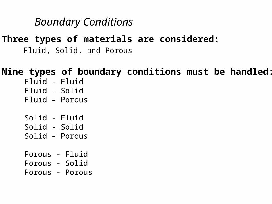
Boundary Conditions
Three types of materials are considered: Fluid, Solid, and Porous
Nine types of boundary conditions must be handled: Fluid - Fluid Fluid - Solid Fluid – Porous
Solid - Fluid Solid - Solid Solid – Porous
Porous - Fluid Porous - Solid Porous - Porous

An Example: Fluid – Porous
)(
)(
)()(
)()(
0
)(
)(
)(
)()1(
)()1(
)()1()()1(
)()1()()1(
)()(
)()(
)()(
jj
jj
jjjj
jjjj
jj
jj
jj
r
rp
rpr
rwru
r
r
ru

Ordinary Reflection and Transmission Coefficients
c+(j +1) = T+
(j )c+(j ) + R
( j )c-( j+1)c-
( j ) = R( j )c+
( j) + T-( j)c-
( j+1
j+1j
c-( j +1)
c+(j )
R( j )c+
(j )
T-( j)c-
( j+1)
T+( j)c+
( j)
R ( j )c-
( j +1)
c( j) R
( j )c( j) T
( j)c( j1)
c( j1) T
( j)c( j ) R
( j)c( j1)

)1()(1)1()(
)()(
)()(
jjjj
jj
jj
EEEERT
TR
They can be directly calculated from
)()()()()( jjjjj cEcEu

Generalized Reflection and Transmission Coefficients
)()()( ˆ jjj cRc
)()()1( ˆ jjj
cTc
c + ( j )
c - ( j ) = ̂ R 1
( j ) c + ( j )
c + ( j + 1 ) = ̂ T
+ ( j ) c
+ ( j )
j j+1 j+2
)()1()()()(
)(1)1()()(
ˆˆˆ
]ˆ[ˆ
jjjjj
jjjj
TRTRR
TRRIT
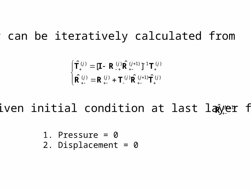
They can be iteratively calculated from
with given initial condition at last layer for )1(ˆ NR
1. Pressure = 02. Displacement = 0

Normal Modes and Resonance Frequencies
The normal modes are the non-trivial solutions of the source-free wave equation under given boundary conditions. The requirement of a non-trivial solution leads to the dispersion relation:
Its solution, for a model m, gives the resonance frequency.
0mRI |),(ˆ| )1(

Pressure in Empty Cavity of the First Mode
Radius (m)
Vp (m/s)
Density (kg/m3) f(1) (Hz) f(2)
(Hz) f(3) (Hz)
0.6 984 1000 1000.13 1831.17 2655.43
Cavity Parameters (Zero displacement on cavity wall)
Test Examples

First 3 Resonance Frequencies of an Empty Cavity
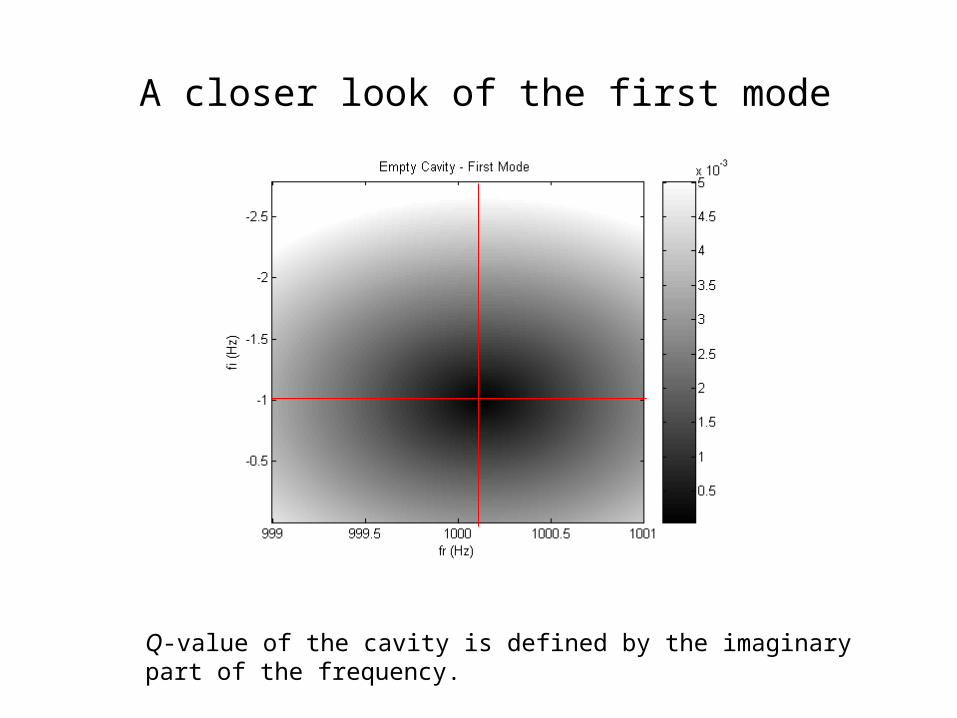
Q-value of the cavity is defined by the imaginary part of the frequency.
A closer look of the first mode

Sample Type
Thickness of elastic coating layer (mm)
Vs (m/s)
Permeability(mDarcy)
Porosity(%)
f(1)
(Hz)f(2)
(Hz)f(3)
(Hz)
Acoustic - - - - 1012.38 1868.39 2726.53
Elastic - 1650 - - 1011.85 1866.87 2723.74
Poroelastic - 1650 370 21 1010.62 1864.31 2719.84
Poroelastic - 1650 600 21 1010.27 1863.59 2719.037
Poroelastic - 1650 1370 21 1009.83 1861.67 2716.17
Poroelastic - 1650 6000 21 1009.68 1859.95 2709.14
Poroelastic 5 1650 1370 21 1011.73 1866.50 2723.05
Poroelastic 1 1650 1370 21 1011.69 1866.40 2722.89
Poroelastic 0.1 1650 1370 21 1011.69 1866.38 2722.84
Simulation results for 4 types of 7 samples (Berea)

1009.6
1009.8
1010
1010.2
1010.4
1010.6
1010.8
2.5 3 3.5 4
log(perm) (mD)
Fre
quen
cy (
Hz)
Resonance frequency changes vs. permeability (4 open porous samples)
Applications
• Verification of perturbation theory
• Comparison with diffusion model for porous samples
• Estimation of Vp & Vs with DARS

AV
V
f
ff
s
c
21
21
22
112 /)(
Estimation of Compressibility Using Perturbation Theory
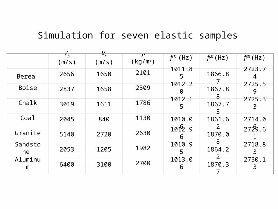
Vp (m/s) Vs (m/s) (kg/m3) f(1) (Hz) f(2)
(Hz) f(3) (Hz)
Berea 2656 1650 2101 1011.85 1866.87 2723.74
Boise 2837 1658 2309 1012.20 1867.88 2725.59
Chalk 3019 1611 1786 1012.15 1867.73 2725.33
Coal 2045 840 1130 1010.06 1861.62 2714.06
Granite 5140 2720 2630 1012.96 1870.08 2729.61
Sandstone 2053 1205 1982 1010.95 1864.22 2718.83
Aluminum 6400 3100 2700 1013.06 1870.37 2730.13
Simulation for seven elastic samples

Given(GPa)-1
Estimated(GPa)-1
Error (%)
Berea 0.1390 0.1322 -4.9
Boise 0.09880 0.09790 -0.9
Chalk 0.09903 0.1030 4.0
Coal 0.2730 0.3982 13
Granite 0.02297 0.02302 0.2
Sandstone 0.2214 0.2214 0
Aluminum 0.01316 0.01316 0
Compressibility estimated with the perturbation formula

Comparison with Diffusion Model for Porous Samples
01
2
2
Pr
P
rr
P
ki f /
}][
][2Re{)1(
0
0 00
02
0r
fme rdrrJ
rJ
r

BereaPerm
(mDarcy)
(%)m -Given
(GPa)-1
e1 -Diffusion
(GPa)-1
e2 –DARS
(GPa)-1
Elastic - - 0.1390 0.1322 - -
Porous 370 21 0.1390 0.250545 0.254153 -1.4%
Porous 600 21 0.1390 0.285355 0.288843 -1.2%
Porous 1370 21 0.1390 0.318042 0.332504 -4.3%
Porous 6000 21 0.1390 0.328275 0.347402 -5.5%
2
21
e
ee
Parameter estimation of Berea samples using different methods (Same porosity but different permeability)
Biot model, Diffusion Model, Slow Wave
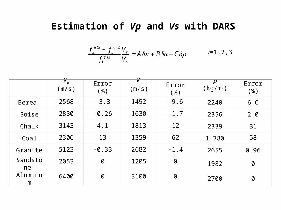
Estimation of Vp and Vs with DARS
CBAV
V
f
ff
s
ci
ii
2)(1
2)(1
2)(2
Vp (m/s) Error (%) Vs (m/s) Error (%) (kg/m3) Error (%)
Berea 2568 -3.3 1492 -9.6 2240 6.6
Boise 2830 -0.26 1630 -1.7 2356 2.0
Chalk 3143 4.1 1813 12 2339 31
Coal 2306 13 1359 62 1.780 58
Granite 5123 -0.33 2682 -1.4 2655 0.96
Sandstone 2053 0 1205 0 1982 0
Aluminum 6400 0 3100 0 2700 0
i=1,2,3
Remarks
• This simulation tool can also be used for other studies, e.g., the empirical equations for Q-value estimation.
• Boit model and the diffusion model are consistent in our case.