Embed Size (px)
Citation preview
A C O U S T I C P E R F O R M A N C E O F B I A S F L O WL I N E R S I N G A S T U R B I N E C O M B U S T O R S
claus lahiri

D I S S E RTAT I O N
A C O U S T I C P E R F O R M A N C E O F B I A S F L O WL I N E R S I N G A S T U R B I N E C O M B U S T O R S
vorgelegt vonDipl.-Ing. Claus Lahiri
geb. in Bergisch Gladbach
von der Fakultät V - Verkehrs- und Maschinensystemeder Technischen Universität Berlin
zur Erlangung des akademischen Grades
Doktor der Ingenieurwissenschaften– Dr.-Ing. –
genehmigte Dissertation
Berlin 2014
Promotionsausschuss:
Vorsitzender: Prof. Dr.-Ing. Dieter PeitschGutachter: Prof. Dr. rer. nat. Lars EnghardtGutachter: Prof. Dr. Tech. Hans Bodén
Tag der wissenschaftlichen Aussprache: 25. November 2014

© claus lahiri, 2014
A B S T R A C T
Thermoacoustic instabilities prevent the implementation of mod-ern combustion concepts in gas turbines, which are essential forhigher efficiency and lower emissions. Bias flow liners are able tosuppress these instabilities by increasing the acoustic losses of thesystem. However, it is an open question under which conditionstheir full potential can be retrieved.
This thesis collects the available information concerning theacoustic properties of bias flow liners and puts it into perspec-tive for the application in a gas turbine combustor. The reviewincludes a rigorous assessment of the existing models. The mod-els and previous findings are evaluated by comparing them to theresults of a comprehensive experimental study regarding the rel-evant acoustic, geometric, thermodynamic, and flow parameters.This includes for the first time the influence of pressure and tem-perature.
The results reveal that there is a resonance dominated regimeat low bias flow Mach numbers with rather complex parameterdependencies and a bias flow dominated regime which is mainlydependent on three parameters only: the bias flow, the porosity,and a resonance parameter.

Z U S A M M E N FA S S U N G
Der Einsatz moderner Verbrennungskonzepte zur Effizienzsteige-rung und Schadstoffreduktion bei Gasturbinen wird oft durchthermo-akustische Instabilitäten verhindert. Durchströmte Brenn-kammerliner können die akustische Dämpfung des Systems er-höhen und die Instabilitäten unterdrücken. Eine wesentliche Fra-ge ist, bei welchen Parametereinstellungen eine optimale Dämp-fungswirkung erzielt werden kann.
Diese Arbeit liefert eine umfassende Übersicht der bisherigenForschung. In einer experimentellen Studie werden akustische,geometrische, thermodynamische und strömungsmechanische Pa-rameter untersucht. Zum ersten Mal wird hier auch der Einflussvon Druck und Temperatur durch eine Messung abgebildet. Dieseweitreichende Datenbasis ermöglicht eine detaillierte Bewertungder einzelnen Parameter und der Qualität der Modelle.
Die Ergebnisse zeigen einen Betriebsbereich bei langsamen Ge-schwindigkeiten der von Resonanzen dominiert ist und kompli-zierte Parameterabhängigkeiten aufweist. Bei höheren Geschwin-digkeiten dominiert die Durchströmung und die Schallabsorptionist im Wesentlichen von nur drei Parametern abhängig: Porosität,Durchströmungsgeschwindigkeit und einem Resonanzparameter.

C O N T E N T S
1 introduction 11.1 Motivation . . . . . . . . . . . . . . . . . . . . . . . . . 71.2 Outline . . . . . . . . . . . . . . . . . . . . . . . . . . . 8
2 bias flow liners 112.1 Combustor Liner . . . . . . . . . . . . . . . . . . . . . 11
2.1.1 Parameter Overview 152.2 Geometry Parameters . . . . . . . . . . . . . . . . . . 16
2.2.1 Orifice Geometry 17 – 2.2.2 Perforation Geometry 20 –2.2.3 Cavity Geometry 24
2.3 Thermodynamic Parameters . . . . . . . . . . . . . . . 262.3.1 Temperature 26 – 2.3.2 Pressure 27
2.4 Acoustic Parameters . . . . . . . . . . . . . . . . . . . 272.4.1 Frequency 27 – 2.4.2 Amplitude / Sound Pressure Level 28
2.5 Flow Parameters . . . . . . . . . . . . . . . . . . . . . 322.5.1 Grazing Flow 32 – 2.5.2 Bias Flow 33
3 literature on bias flow liners 433.1 Bias Flow as a Concept of Impedance Control . . . . 433.2 Sound Absorption due to Vorticity Shedding . . . . . 453.3 Recent Developments . . . . . . . . . . . . . . . . . . . 493.4 Chronological Overview . . . . . . . . . . . . . . . . . 52
4 modeling of bias flow liners 574.1 Rayleigh Conductivity . . . . . . . . . . . . . . . . . . 574.2 Acoustic Impedance . . . . . . . . . . . . . . . . . . . 59
4.2.1 Impedance Modeling of Perforations 61 – 4.2.2 GrazingFlow Impedance 67 – 4.2.3 Bias Flow Impedance 67
4.3 Howe Rayleigh Conductivity Model . . . . . . . . . . 684.4 Jing Model (Modified Howe Model) . . . . . . . . . . 714.5 Luong Model (Simplified Howe Model) . . . . . . . . 73
x contents
4.6 Bauer Impedance Model . . . . . . . . . . . . . . . . . 734.7 Betts Impedance Model . . . . . . . . . . . . . . . . . 754.8 Bellucci Impedance Model . . . . . . . . . . . . . . . . 764.9 Application to a Cylindrical Geometry . . . . . . . . . 79
4.9.1 Transfer Matrix Method 80 – 4.9.2 Eldredge & DowlingMethod 85
4.10 Some Comparisons . . . . . . . . . . . . . . . . . . . . 894.10.1 Impedance Models 89 – 4.10.2 Transfer Matrix Methodvs. Eldredge & Dowling Method 93 – 4.10.3 Howe vs. Luong 95
5 duct acoustics 975.1 Acoustic Wave Equation . . . . . . . . . . . . . . . . . 975.2 Three-Dimensional Waves . . . . . . . . . . . . . . . . 101
5.2.1 Cut-On Frequency 104 – 5.2.2 Evanescent Modes 105 –5.2.3 Resonances in an Annular Cavity 108
5.3 Plane Waves . . . . . . . . . . . . . . . . . . . . . . . . 1095.4 Attenuation of Sound . . . . . . . . . . . . . . . . . . . 111
5.4.1 Losses at the Wall 114 – 5.4.2 Losses due to Turbulent Flow126 – 5.4.3 Losses Within the Fluid 130
6 experimental method & analysis 1396.1 Spectral Analysis . . . . . . . . . . . . . . . . . . . . . 140
6.1.1 Welch Method 140 – 6.1.2 Rejection of Flow Noise 1436.2 Plane Wave Decomposition . . . . . . . . . . . . . . . 1446.3 Reflection and Transmission Coefficients . . . . . . . 1516.4 Dissipation Coefficient . . . . . . . . . . . . . . . . . . 154
6.4.1 Average Dissipation Coefficient 155 – 6.4.2 DissipationError 156 – 6.4.3 Compared to the Absorption Coefficient 156
6.5 Duct Acoustic Test Rig . . . . . . . . . . . . . . . . . . 1596.5.1 Setup & Instrumentation 159 – 6.5.2 Microphone Calibra-tion 162 – 6.5.3 End-Reflections 165 – 6.5.4 Influence of Evanes-cent Modes 165 – 6.5.5 Accuracy 170
6.6 Hot Acoustic Test Rig . . . . . . . . . . . . . . . . . . . 1716.6.1 Setup & Instrumentation 172 – 6.6.2 Air Supply 177 –6.6.3 Microphone Probes 183 – 6.6.4 Estimation of the Humidity189 – 6.6.5 Attenuation at Elevated Pressure and Temperature190 – 6.6.6 Accuracy 193
contents xi
7 parameter study 1957.1 Sound Pressure Level . . . . . . . . . . . . . . . . . . . 1957.2 Bias Flow . . . . . . . . . . . . . . . . . . . . . . . . . . 2047.3 Grazing Flow . . . . . . . . . . . . . . . . . . . . . . . 2137.4 Simultaneous Grazing & Bias Flow . . . . . . . . . . . 2197.5 Porosity . . . . . . . . . . . . . . . . . . . . . . . . . . . 2227.6 Wall Thickness . . . . . . . . . . . . . . . . . . . . . . . 2287.7 Orifice Cross-Section Shape . . . . . . . . . . . . . . . 2317.8 Orifice Edge Geometry . . . . . . . . . . . . . . . . . . 2367.9 Orifice Angle . . . . . . . . . . . . . . . . . . . . . . . 2417.10 Double-Skin Configuration . . . . . . . . . . . . . . . 2477.11 Cavity Volume . . . . . . . . . . . . . . . . . . . . . . . 2497.12 Partitioned Cavity . . . . . . . . . . . . . . . . . . . . . 2537.13 Perforation Placement . . . . . . . . . . . . . . . . . . 2557.14 Perforation Pattern . . . . . . . . . . . . . . . . . . . . 2607.15 Temperature . . . . . . . . . . . . . . . . . . . . . . . . 2647.16 Pressure . . . . . . . . . . . . . . . . . . . . . . . . . . 2697.17 Strouhal Number . . . . . . . . . . . . . . . . . . . . . 271
8 concluding remarks 275
A properties of air 283A.1 Equations of Ideal Gas Properties . . . . . . . . . . . . 283A.2 Ideal Gas vs. Real Gas . . . . . . . . . . . . . . . . . . 284A.3 Tables of Real Gas Properties . . . . . . . . . . . . . . 285
B some mathematics 293B.1 Rayleigh Conductivity and Impedance . . . . . . . . 293B.2 Conversion of Transfer Matrix into Scattering Matrix 294
bibliography 297

L I S T O F S Y M B O L S
latin symbols
A AmplitudeA Cross-section areaAopen Liner total open areaArel Relative errora Attenuation rateB Complex stagnation enthalpy amplitudeB′ Fluctuating stagnation enthalpyC Acoustic complianceC CircumferenceCc Contraction coefficientCd Discharge coefficientCr Resistance coefficientCv Velocity coefficientc Speed of soundcp Specific heat capacity at constant pressurecph Phase velocitycv Specific heat capacity at constant volumeD Duct diameterD Energy dissipation coefficientDc Cavity diameterDh Hydraulic diameterd Orifice diameterdc Cavity depthe Exponential functionerr Fit errorerr Average fit error over all microphonesf Darcy friction factorf Frequencyfc,mn Cut-on frequency of mode m:n
xiv list of symbols
fr Resonance frequencyfr,i Vibrational relaxation frequency of constituent iGxx One-sided auto-spectral densityGxy One-sided cross-spectral densityHe Helmholtz numberHm Hankel function of order mh Humidity as molar concentration of water vaporIm{z} Imaginary part of complex number zIm Modified Bessel function of the first kind of order mi Imaginary unitJm Bessel function of the first kind of order mjmn Eigenvalue of JmKm Modified Bessel function of the second kind of order mKR Rayleigh conductivityk Wave numberk± Convective wave numberk0 Free field wave numberkr,mn Radial wave number of mode m:nks Stokes wave numberk′s Effective Stokes wave numberkx,mn Axial wave number of mode m:nL LengthL Perforation lengthLc Cavity lengthLeff Effective perforation lengthl Orifice lengthl′ Length end correctionleff Effective orifice lengthM Acoustic inertanceM Mach numberMb Bias flow Mach numberMb Mean orifice bias flow Mach numberMg Grazing flow Mach numberm Circumferential mode orderm Mass flow rate
list of symbols xv
mb Bias flow mass flow ratemg Grazing flow mass flow raten Radial mode orderP Acoustic powerP Acoustic energy fluxP Perimeterp Pressurep0 Mean pressurep∗ Critical pressurep′ Acoustic pressurep Complex pressure amplitudepc Pressure at the critical point of waterpmn Complex amplitude of mode m:npref Reference pressurepws Saturation water vapor pressurePr Prandtl numberPrt Turbulence Prandtl numberQ Resonance parameterQ′ Heat release fluctuationQmn Hard-wall Eigenvalue of Ym
q Acoustic volume velocityq Complex volume velocity amplitudeR Acoustic resistanceR Duct radiusR Energy reflection coefficientR Specific gas constantR RadiusRc Cavity radiusRe{z} Real part of complex number zRe Reynolds numberRec Critical Reynolds number for pipe flowRH Relative humidityr Orifice radiusr Radial coordinater Specific acoustic resistance
xvi list of symbols
r Amplitude reflection coefficientre Amplitude end-reflection coefficientrh Hydraulic radiusS Scattering matrixSxy Scattering matrix elementSh Shear numberSt Strouhal numbers Entropys Spacing between microphoness Spacing between orificess′ Entropy fluctuationssθ Spacing between orifices in circumferential directionsx Spacing between orifices in axial directionT Energy transmission coefficientT ′ Fluctuating temperatureT TemperatureT Transfer matrixTa Constant, see Tab. A.1Tb Constant, see Tab. A.1Tc Temperature at the critical point of waterTd Temperature at dew pointTref Reference temperatureTs Sutherland constantTxy Transfer matrix elementt Timet Wall thicknesst Amplitude transmission coefficientTL Transmission lossU Mean flow velocityUb Bias flow velocityUb Mean orifice bias flow velocityUg Grazing flow velocityV Cavity volumev Velocityv∗ Friction velocity
list of symbols xvii
v0 Mean velocityv′ Acoustic particle velocityv Complex velocity amplitudev Acoustic mass velocityv Complex mass velocity amplitudew Window functionX Acoustic reactanceXi Mole fraction of constituent ix Specific acoustic reactancex Axial coordinateY Wall shear layer admittanceYm Bessel function of the second kind of order my Transverse coordinateZ Acoustic impedance based on the mass velocityZ Acoustic impedanceZ0 Characteristic acoustic impedance of a lumped elementZrot Rotational collision numberz Specific acoustic impedancez0 Characteristic acoustic impedance
greek symbols
α Orifice pitch angleα Absorption coefficientα Attenuation coefficientα± Convective attenuation coefficientα Average convective attenuation coefficientβ Coefficient of thermal expansionχ Normalized specific acoustic reactanceχ Thermal diffusivityδ Imaginary part of the Rayleigh conductivityδ Boundary layer thicknessδτ Thickness of the viscous sublayer of turbulent flowδν Thickness of the viscous acoustic boundary layerδχ Thickness of the thermal acoustic boundary layerδij Kronecker delta
xviii list of symbols
∆cph Change of phase velocity∆P Bias flow pressure drop∆Pt Bias flow total pressure drop in a double-skin configurationη Complianceη Hub-to-tip ratio in an annular ductΓ Propagation constantγxy Coherenceγ Heat capacity ratioγ Real part of the Rayleigh conductivityκ Kármán constantκ Thermal conductivityλ Ratio of bias flow to grazing flowλ Second viscosity coefficientλ Wavelengthµ Dynamic viscosityµB Bulk viscosity (also called volume viscosity)ν Kinematic viscosityν′ Effective kinematic viscosity including thermal conductivity
lossesπ Mathematical constantΦ Acoustic lossesϕ Phase angleφ Viscous dissipation rateθ Circumferential coordinateθ Normalized specific acoustic resistanceθi Characteristic vibrational temperature of constituent iρ Densityρ′ Fluctuating densityρ0 Mean densityσ Perforation porosityτij Viscous stress tensorω Angular frequencyψ Fok functionζ Normalized specific acoustic impedance
list of symbols xix
superscripts
+ in positive x-direction, in flow direction− in negative x-direction, against flow direction
subscripts
1 Section 12 Section 2a Excitation Aac regarding the acoustic modeb Excitation Bcl regarding classical, i. e. viscothermal, losses within the fluidcr regarding classical and rotational relaxation losses within
the fluident regarding the entropy modefluid regarding losses within the fluidrot regarding rotational relaxation losses within the fluidtotal regarding total lossesturb regarding viscothermal and turbulence losses at the wallvib regarding vibrational relaxation losses within the fluidvor regarding the vorticity modewall regarding viscothermal losses at the wall
acronyms
DDOF Double-Degree-of-Freedom (also: 2DOF)DLR Deutsches Zentrum für Luft- und RaumfahrtDUCT-C Duct Acoustic Test Rig - Circular Cross-SectionEDM Eldredge and Dowling MethodHAT Hot Acoustic Test RigISA International Standard AtmosphereICAO International Civil Aviation OrganizationISO International Organization for StandardizationSDOF Single-Degree-of-FreedomSNR Signal-to-noise ratioSPL Sound Pressure LevelTMM Transfer Matrix Method


1I N T R O D U C T I O N
Gas turbines convert the chemical energy inherent in a gaseousor liquid fuel into mechanical energy. Depending on their applica-tion they are designed to deliver shaft power or thrust, for exam-ple to generate electricity in a power plant or as aircraft propul-sion, respectively.
6 115 TWh 22 126 TWh
Other0.6%Hydro
21.0%
Nuclear3.3%
Natural gas12.2%
Oil 24.6%
Coal/ peat38.3%
Other4.5%
Nuclear11.7%
Oil 4.8%
Coal/ peat41.3%
Natural gas21.9%
Hydro15.8%
1973 2011
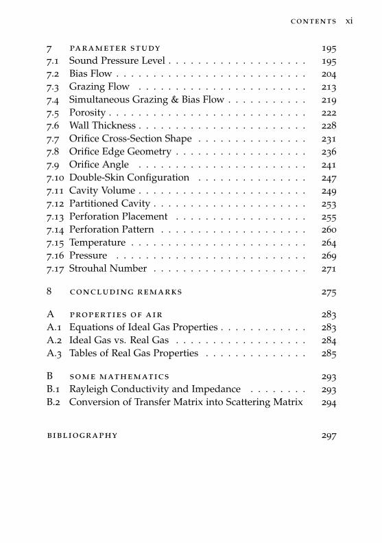
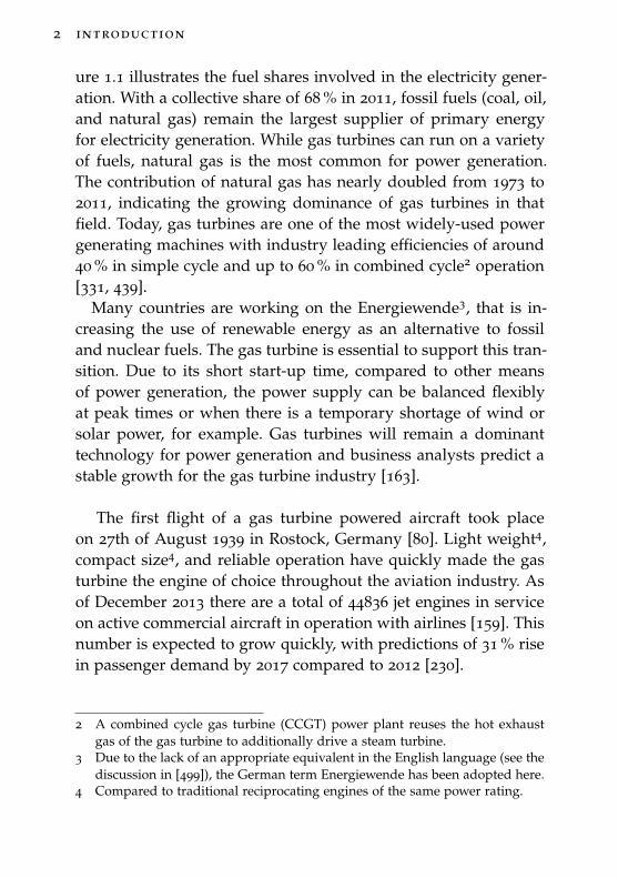
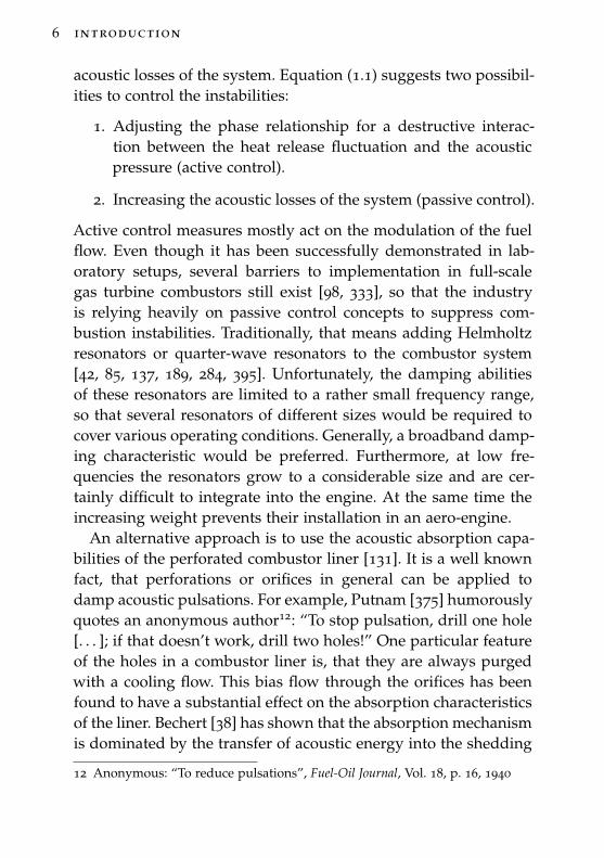
Figure 1.1: 1973 and 2011 fuel shares of electricity generation. (KeyWorld Energy Statistics © OECD/IEA, 2013 [231])
The energy industry relies heavily on gas turbines for electric-ity production. The global electricity consumption has more thantripled from 439 Mtoe1 in 1973 to 1582 Mtoe in 2011 [231]. Fig-
1 Million tonnes of oil equivalent, 1 Mtoe = 11630 GWh [231].
2 introduction
ure 1.1 illustrates the fuel shares involved in the electricity gener-ation. With a collective share of 68 % in 2011, fossil fuels (coal, oil,and natural gas) remain the largest supplier of primary energyfor electricity generation. While gas turbines can run on a varietyof fuels, natural gas is the most common for power generation.The contribution of natural gas has nearly doubled from 1973 to2011, indicating the growing dominance of gas turbines in thatfield. Today, gas turbines are one of the most widely-used powergenerating machines with industry leading efficiencies of around40 % in simple cycle and up to 60 % in combined cycle2 operation[331, 439].
Many countries are working on the Energiewende3, that is in-creasing the use of renewable energy as an alternative to fossiland nuclear fuels. The gas turbine is essential to support this tran-sition. Due to its short start-up time, compared to other meansof power generation, the power supply can be balanced flexiblyat peak times or when there is a temporary shortage of wind orsolar power, for example. Gas turbines will remain a dominanttechnology for power generation and business analysts predict astable growth for the gas turbine industry [163].
The first flight of a gas turbine powered aircraft took placeon 27th of August 1939 in Rostock, Germany [80]. Light weight4,compact size4, and reliable operation have quickly made the gasturbine the engine of choice throughout the aviation industry. Asof December 2013 there are a total of 44836 jet engines in serviceon active commercial aircraft in operation with airlines [159]. Thisnumber is expected to grow quickly, with predictions of 31 % risein passenger demand by 2017 compared to 2012 [230].
2 A combined cycle gas turbine (CCGT) power plant reuses the hot exhaustgas of the gas turbine to additionally drive a steam turbine.
3 Due to the lack of an appropriate equivalent in the English language (see thediscussion in [499]), the German term Energiewende has been adopted here.
4 Compared to traditional reciprocating engines of the same power rating.
introduction 3
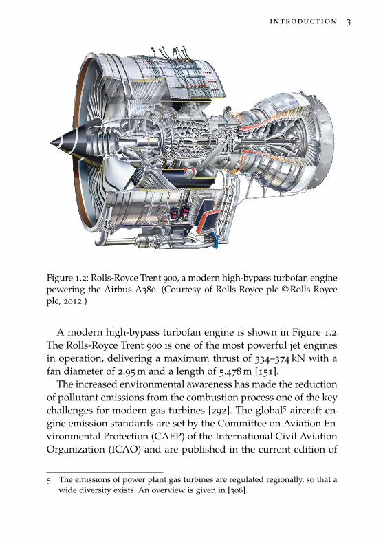
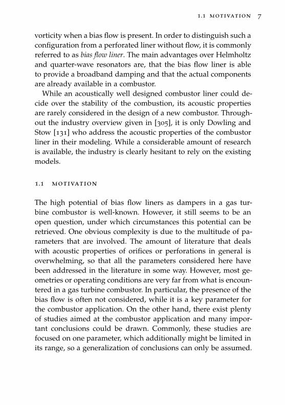
Figure 1.2: Rolls-Royce Trent 900, a modern high-bypass turbofan enginepowering the Airbus A380. (Courtesy of Rolls-Royce plc © Rolls-Royceplc, 2012.)
A modern high-bypass turbofan engine is shown in Figure 1.2.The Rolls-Royce Trent 900 is one of the most powerful jet enginesin operation, delivering a maximum thrust of 334–374 kN with afan diameter of 2.95 m and a length of 5.478 m [151].
The increased environmental awareness has made the reductionof pollutant emissions from the combustion process one of the keychallenges for modern gas turbines [292]. The global5 aircraft en-gine emission standards are set by the Committee on Aviation En-vironmental Protection (CAEP) of the International Civil AviationOrganization (ICAO) and are published in the current edition of
5 The emissions of power plant gas turbines are regulated regionally, so that awide diversity exists. An overview is given in [306].
4 introduction
Annex 16, Volume 2. The Advisory Council for Aviation Researchand Innovation in Europe (ACARE) has formulated future goalsfor the emissions of carbon dioxide CO2 and nitrogen oxide6 NOx
in their Vision 2020 [4] and Flightpath 2050 [5] reports. It shouldbe aimed for a reduction in CO2 of 50 % and 75 % and NOx of80 % and 90 % until 2020 and 20507, respectively. The amount ofCO2 in the exhaust gases is directly related to the combustion effi-ciency [292], so that the levels have been reduced continuously, inline with the optimization for low fuel consumption. The primefactor in reducing NOx is to lower the flame temperature8, whichadversely affects the efficiency and the CO2 production. Thus, thereduction of NOx is a major concern throughout the gas turbineindustry, including both aviation and power.
This problem is addressed by modern combustion concepts,which operate in the lean regime. The lean combustion increasesthe air-fuel-ratio beyond the stoichiometric mixture9, i. e. more air,relative to the fuel, is taking part in the combustion. As a result,the flame temperature is lowered and NOx production is reduced.Particularly rewarding is the lean pre-mixed/pre-vaporized com-bustion (LPP) [292].
However, the implementation of this concept is often preventedby its tendency to promote combustion instabilities. Combustioninstabilities are pressure pulsations resulting from a thermoacous-tic feedback between the heat release of the flame and acousticpressure oscillations. The instabilities lead to excessive wearingor even cracking of exposed components within or adjacent tothe combustor. High amplitude instabilities can result in a flameblow-off or in the immediate and fatal damage of components, po-
6 This collectively includes nitrogen monoxide NO and nitrogen dioxide NO2.7 These values are relative to the capabilities of a typical new aircraft in the
year 2000.8 Two additional factors are a uniform temperature distribution and a short
residence time.9 A stoichiometric mixture contains sufficient oxygen for a complete combus-
tion of the available fuel.
introduction 5
tentially releasing detached pieces into the turbine downstream.Low amplitude instabilities require an increased downtime of gasturbines for inspections and repairs if necessary. The maintenancecosts that can be directly associated with damages due to com-bustion instabilities exceed $1 billion annually [305]. Furthermore,combustion instabilities are not limited to gas turbines, but are awidespread problem in combustion systems, e. g. liquid and solidpropellant rocket engines [102, 190, 497], ramjet engines [102, 440],afterburners of turbojet engines [67, 102], and domestic or indus-trial furnaces [375].
The process leading up to an instability is not yet fully under-stood. Thus, it is not possible to predict the occurrence of insta-bility or avoid it in the first place. Lieuwen and Yang [305] givean overview of the recent situation and mitigation strategies inthe gas turbine industry. Commonly, thermoacoustic instabilitiesoccur at one dominant frequency, which is mainly dependent onthe combustor geometry and the operating condition. The gen-eral mechanism can be described as follows: The oscillating heatrelease of the flame produces sound, which is reflected at the com-bustor boundary, feeding back to the heat release oscillation. Thisfeedback loop in itself does not necessarily lead to instability, thecombustion becomes unstable only when the heat release fluctua-tion and the acoustic pressure oscillations are in phase ([388, 390]).This necessary condition is referred to as Rayleigh criterion10. Inmathematical terms, instability does occur when [376]11∫
T
p′(t)Q′(t)dt > Φ, (1.1)
where T is the period of one oscillation, p′ is the acoustic pressurefluctuation, Q′ is the heat release fluctuation, and Φ describes the
10 Named after John William Strutt, Lord Rayleigh (1842-1919, English physi-cist).
11 The original derivation by Putnam and Dennis [376] neglects the acousticlosses, so that Φ = 0. The expression including the acoustic losses can befound in [238, 506], for example.
6 introduction
acoustic losses of the system. Equation (1.1) suggests two possibil-ities to control the instabilities:
1. Adjusting the phase relationship for a destructive interac-tion between the heat release fluctuation and the acousticpressure (active control).
2. Increasing the acoustic losses of the system (passive control).
Active control measures mostly act on the modulation of the fuelflow. Even though it has been successfully demonstrated in lab-oratory setups, several barriers to implementation in full-scalegas turbine combustors still exist [98, 333], so that the industryis relying heavily on passive control concepts to suppress com-bustion instabilities. Traditionally, that means adding Helmholtzresonators or quarter-wave resonators to the combustor system[42, 85, 137, 189, 284, 395]. Unfortunately, the damping abilitiesof these resonators are limited to a rather small frequency range,so that several resonators of different sizes would be required tocover various operating conditions. Generally, a broadband damp-ing characteristic would be preferred. Furthermore, at low fre-quencies the resonators grow to a considerable size and are cer-tainly difficult to integrate into the engine. At the same time theincreasing weight prevents their installation in an aero-engine.
An alternative approach is to use the acoustic absorption capa-bilities of the perforated combustor liner [131]. It is a well knownfact, that perforations or orifices in general can be applied todamp acoustic pulsations. For example, Putnam [375] humorouslyquotes an anonymous author12: “To stop pulsation, drill one hole[. . . ]; if that doesn’t work, drill two holes!” One particular featureof the holes in a combustor liner is, that they are always purgedwith a cooling flow. This bias flow through the orifices has beenfound to have a substantial effect on the absorption characteristicsof the liner. Bechert [38] has shown that the absorption mechanismis dominated by the transfer of acoustic energy into the shedding
12 Anonymous: “To reduce pulsations”, Fuel-Oil Journal, Vol. 18, p. 16, 1940
1.1 motivation 7
vorticity when a bias flow is present. In order to distinguish such aconfiguration from a perforated liner without flow, it is commonlyreferred to as bias flow liner. The main advantages over Helmholtzand quarter-wave resonators are, that the bias flow liner is ableto provide a broadband damping and that the actual componentsare already available in a combustor.
While an acoustically well designed combustor liner could de-cide over the stability of the combustion, its acoustic propertiesare rarely considered in the design of a new combustor. Through-out the industry overview given in [305], it is only Dowling andStow [131] who address the acoustic properties of the combustorliner in their modeling. While a considerable amount of researchis available, the industry is clearly hesitant to rely on the existingmodels.
1.1 motivation
The high potential of bias flow liners as dampers in a gas tur-bine combustor is well-known. However, it still seems to be anopen question, under which circumstances this potential can beretrieved. One obvious complexity is due to the multitude of pa-rameters that are involved. The amount of literature that dealswith acoustic properties of orifices or perforations in general isoverwhelming, so that all the parameters considered here havebeen addressed in the literature in some way. However, most ge-ometries or operating conditions are very far from what is encoun-tered in a gas turbine combustor. In particular, the presence of thebias flow is often not considered, while it is a key parameter forthe combustor application. On the other hand, there exist plentyof studies aimed at the combustor application and many impor-tant conclusions could be drawn. Commonly, these studies arefocused on one parameter, which additionally might be limited inits range, so a generalization of conclusions can only be assumed.
8 introduction
It seems to be necessary to take a step back and look at thebroader picture. The scattered fragments of information need tobe collected and put into perspective. However, the available ex-perimental data varies immensely in setup, experimental method,and describing quantities, so that an independent set of data,based on one foundation, is required for the evaluation of theinformation.
The goal of this holistic approach is to identify and determinethe influence of the significant parameters. Furthermore, a com-prehensive assessment of the existing models can be provided, sothat possible improvements can be suggested if necessary.
1.2 outline
Chapter 2 begins with a detailed overview of the liner setup andthe operating conditions within a gas turbine combustor. The rel-evant geometric, thermodynamic, acoustic, and flow parametersare defined with respect to the experiments performed here andput into perspective with the definitions found in the literature.The parameter in focus is the bias flow, so that its definition iscomplemented by a review of the available research involvingbias flow liners in Chapter 3. The various modeling approachesthat are available to predict the acoustic performance of bias flowliners are illustrated in Chapter 4, concluding the review part ofthe thesis.
The second part focuses on the experimental parameter study.Chapter 5 collects the essential theoretical background, which isneeded to understand the acoustic phenomena occurring withina duct. Special attention is put on the various loss mechanisms,that a sound wave experiences when propagating through a hard-walled duct. As will be shown later, these effects become moresignificant at elevated pressure and temperature.Chapter 6 discloses all the details about the realization and theanalysis of the measurements. This includes a detailed description
1.2 outline 9
of the features and properties of the Duct Acoustic Test Rig andthe Hot Acoustic Test Rig, which have both provided their servicesin the parameter study. The results of the study are presented inChapter 7. The influence of each parameter is discussed separately,regarding the current findings as well as previous results fromother studies. When applicable, the models are compared to theexperimental results.

2B I A S F L O W L I N E R S
This chapter takes a detailed look at the setup of typical gas tur-bine combustors and their operating conditions. The parametersthat are relevant for the acoustic performance of a perforated linerare collected and discussed individually. The discussion includesa brief review of the presence and definition of each parameter inthe literature, not limited to combustor liners but for orifices ingeneral. Due to the essential nature of the bias flow in this work,the literature review regarding the bias flow effect receives its owndedicated chapter (see Chapter 3).
2.1 combustor liner
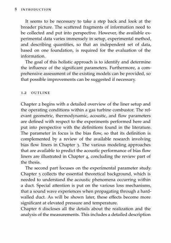
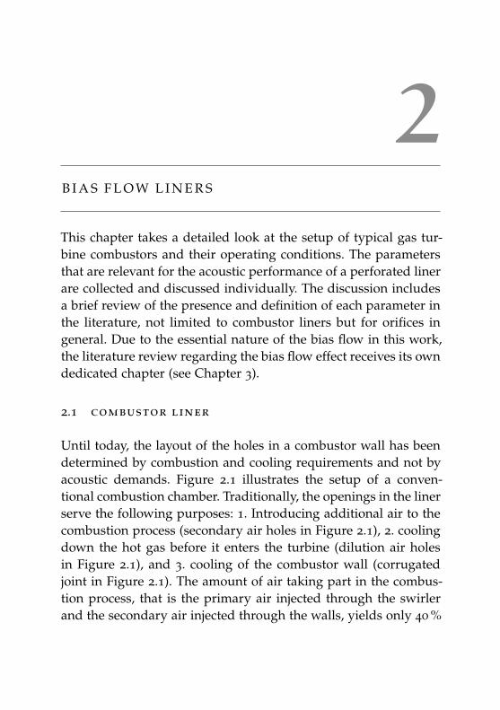
Until today, the layout of the holes in a combustor wall has beendetermined by combustion and cooling requirements and not byacoustic demands. Figure 2.1 illustrates the setup of a conven-tional combustion chamber. Traditionally, the openings in the linerserve the following purposes: 1. Introducing additional air to thecombustion process (secondary air holes in Figure 2.1), 2. coolingdown the hot gas before it enters the turbine (dilution air holesin Figure 2.1), and 3. cooling of the combustor wall (corrugatedjoint in Figure 2.1). The amount of air taking part in the combus-tion process, that is the primary air injected through the swirlerand the secondary air injected through the walls, yields only 40 %
12 bias flow liners
Figure 2.1: Setup of a conventional combustion chamber. (From [408],courtesy of Rolls-Royce plc.)
of the total airflow. The remaining 60 % are required for dilution(20 %) and wall cooling (40 %) [408].
The flow distribution has drastically changed in modern com-bustors. Lean combustion demands more air to take part in thecombustion process. As a consequence, a reduction of cooling airbecame necessary. With novel materials being available and opti-mized cooling techniques, the wall cooling air could be reducedby half to 20 % for combustors that are now in service [292].
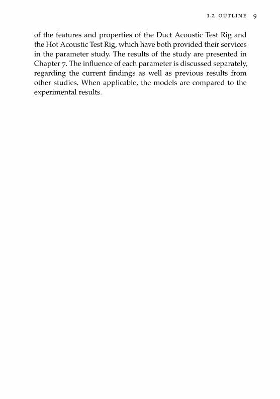
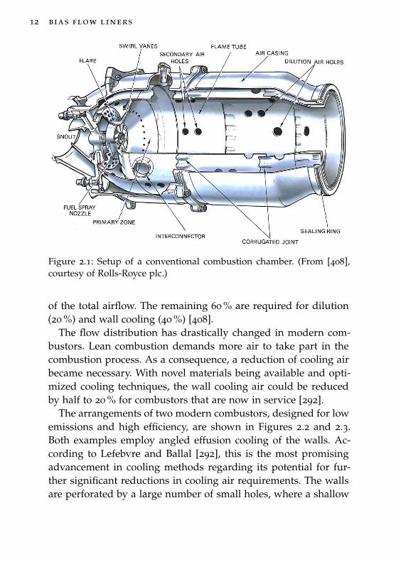
The arrangements of two modern combustors, designed for lowemissions and high efficiency, are shown in Figures 2.2 and 2.3.Both examples employ angled effusion cooling of the walls. Ac-cording to Lefebvre and Ballal [292], this is the most promisingadvancement in cooling methods regarding its potential for fur-ther significant reductions in cooling air requirements. The wallsare perforated by a large number of small holes, where a shallow
2.1 combustor liner 13
Figure 2.2: The GE twin annular premixing swirler (TAPS) combustorwith effusion cooling, designed for low emissions and high efficiency.(From [157], courtesy of General Electric Company.)
angle in combustor mean flow direction provides two advantagesfor the cooling [292]: A larger surface area within the hole forincreased heat removal and the establishment of a cooling filmalong the surface of the wall.
Typical orifice inclination angles are between 20° – 60°. The ori-entation of the cooling orifices might be additionally skewed inthe circumferential direction [92, 253]. The hole diameters rangebetween 0.64-8.82 mm [88]. The cooling efficiency can be furtherincreased by using shaped holes, i. e. holes with an enlarged exitarea where the velocity is reduced and the lateral spreading of thecooling air is improved [178, 183]. A typical wall thickness is inthe range of 0.5-1.5 mm [351].
Generally, the combustor operates at high pressure, high tem-perature, and with a relatively low flow velocity within the cham-ber. Aero-engines are designed to deliver much higher pressure
14 bias flow liners
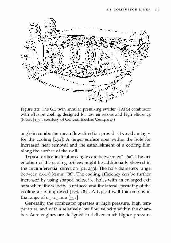
Figure 2.3: View into the annular combustor of the Rolls-Royce E3E Core3/2 technology demonstrator, optimized for lean burn combustion andNOx reduction. (Courtesy of Rolls-Royce plc.)
ratios than stationary gas turbines. Current engine configurationsachieve an overall pressure ratio1 between 30 and 52. For example,the pressure ratio of the Rolls-Royce Trent 900 shown in Figure 1.2is 39. Stationary gas turbines typically operate at pressure ratiosbetween 10 and 25.
A characteristic temperature of a gas turbine is the turbine inlettemperature, that is the temperature of the flow leaving the com-bustor and entering the turbine. While a high turbine inlet temper-ature is desirable from an efficiency point of view, the maximumtemperature is limited by the material properties of the turbineblades and the applied cooling. Currently, temperatures of nearly1900 K can be achieved [331], while typical values are between1300-1700 K [80]. However, the flame temperature within the com-
1 The overall pressure ratio is defined as p3/p1, where p1 is the pressure at theinlet and p3 the pressure delivered to the combustor [408].
2.1 combustor liner 15
buster can be as high as 2200-2600 K [80], with lean burn tempera-tures usually below 2000 K [292]. The cooling air provided by thecompressor is typically between 500-800 K [408].
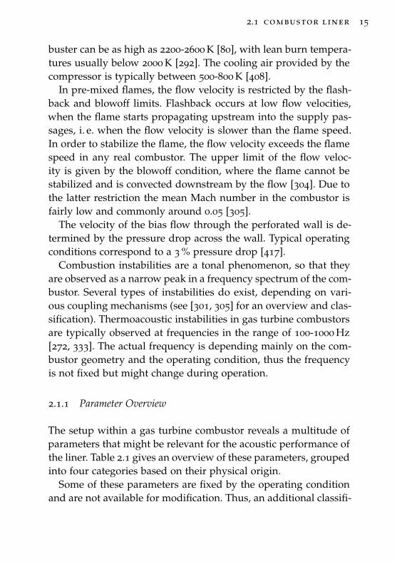
In pre-mixed flames, the flow velocity is restricted by the flash-back and blowoff limits. Flashback occurs at low flow velocities,when the flame starts propagating upstream into the supply pas-sages, i. e. when the flow velocity is slower than the flame speed.In order to stabilize the flame, the flow velocity exceeds the flamespeed in any real combustor. The upper limit of the flow veloc-ity is given by the blowoff condition, where the flame cannot bestabilized and is convected downstream by the flow [304]. Due tothe latter restriction the mean Mach number in the combustor isfairly low and commonly around 0.05 [305].
The velocity of the bias flow through the perforated wall is de-termined by the pressure drop across the wall. Typical operatingconditions correspond to a 3 % pressure drop [417].
Combustion instabilities are a tonal phenomenon, so that theyare observed as a narrow peak in a frequency spectrum of the com-bustor. Several types of instabilities do exist, depending on vari-ous coupling mechanisms (see [301, 305] for an overview and clas-sification). Thermoacoustic instabilities in gas turbine combustorsare typically observed at frequencies in the range of 100-1000 Hz[272, 333]. The actual frequency is depending mainly on the com-bustor geometry and the operating condition, thus the frequencyis not fixed but might change during operation.
2.1.1 Parameter Overview
The setup within a gas turbine combustor reveals a multitude ofparameters that might be relevant for the acoustic performance ofthe liner. Table 2.1 gives an overview of these parameters, groupedinto four categories based on their physical origin.
Some of these parameters are fixed by the operating conditionand are not available for modification. Thus, an additional classifi-
16 bias flow liners
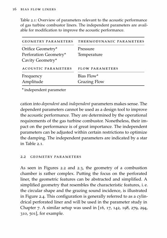
Table 2.1: Overview of parameters relevant to the acoustic performanceof gas turbine combustor liners. The independent parameters are avail-able for modification to improve the acoustic performance.
geometry parameters thermodynamic parameters
Orifice Geometry* PressurePerforation Geometry* TemperatureCavity Geometry*
acoustic parameters flow parameters
Frequency Bias Flow*Amplitude Grazing Flow
* independent parameter
cation into dependent and independent parameters makes sense. Thedependent parameters cannot be used as a design tool to improvethe acoustic performance. They are determined by the operationalrequirements of the gas turbine combustor. Nonetheless, their im-pact on the performance is of great importance. The independentparameters can be adjusted within certain restrictions to optimizethe damping. The independent parameters are indicated by a starin Table 2.1.
2.2 geometry parameters
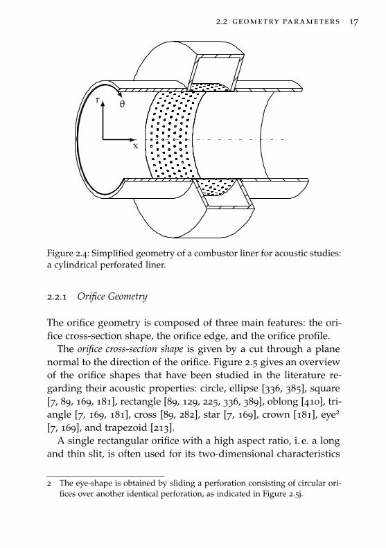
As seen in Figures 2.2 and 2.3, the geometry of a combustionchamber is rather complex. Putting the focus on the perforatedliner, the geometric features can be abstracted and simplified. Asimplified geometry that resembles the characteristic features, i. e.the circular shape and the grazing sound incidence, is illustratedin Figure 2.4. This configuration is generally referred to as a cylin-drical perforated liner and will be used in the parameter study inChapter 7. A similar setup was used in [16, 17, 142, 198, 279, 294,310, 501], for example.
2.2 geometry parameters 17
draft – 2014.06.25 17:29 – claus lahiri
x
r θ
Figure 2.4: Simplified geometry of a combustor liner for acoustic studies:a cylindrical perforated liner.
2.2.1 Orifice Geometry
The orifice geometry is composed of three main features: the ori-fice cross-section shape, the orifice edge, and the orifice profile.
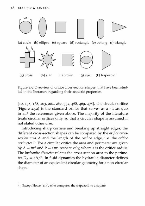
The orifice cross-section shape is given by a cut through a planenormal to the direction of the orifice. Figure 2.5 gives an overviewof the orifice shapes that have been studied in the literature re-garding their acoustic properties: circle, ellipse [336, 385], square[7, 89, 169, 181], rectangle [89, 129, 225, 336, 389], oblong [410], tri-angle [7, 169, 181], cross [89, 282], star [7, 169], crown [181], eye2
[7, 169], and trapezoid [213].A single rectangular orifice with a high aspect ratio, i. e. a long
and thin slit, is often used for its two-dimensional characteristics
2 The eye-shape is obtained by sliding a perforation consisting of circular ori-fices over another identical perforation, as indicated in Figure 2.5j.
18 bias flow liners
draft – 2014.06.25 18:07 – claus lahiri
2r
(a) circle
draft – 2014.06.17 16:00 – claus lahiri
(b) ellipse
draft – 2014.06.17 16:01 – claus lahiri
(c) square
draft – 2014.06.17 16:01 – claus lahiri
(d) rectangle
draft – 2014.06.17 16:01 – claus lahiri
(e) oblong
draft – 2014.06.17 16:01 – claus lahiri
(f) triangle
draft – 2014.06.17 16:01 – claus lahiri
l2l1
(g) cross
draft – 2014.06.17 16:01 – claus lahiri
(h) star
draft – 2014.06.17 16:01 – claus lahiri
(i) crown
draft – 2014.06.17 16:02 – claus lahiri
(j) eye
draft – 2014.06.17 16:02 – claus lahiri
(k) trapezoid
Figure 2.5: Overview of orifice cross-section shapes, that have been stud-ied in the literature regarding their acoustic properties.
[10, 138, 168, 203, 204, 267, 332, 468, 469, 478]. The circular orifice(Figure 2.5a) is the standard orifice that serves as a status quoin all3 the references given above. The majority of the literaturetreats circular orifices only, so that a circular shape is assumed ifnot stated otherwise.
Introducing sharp corners and breaking up straight edges, thedifferent cross-section shapes can be compared by the orifice cross-section area A and the length of the orifice edge, i. e. the orificeperimeter P. For a circular orifice the area and perimeter are givenby A = πr2 and P = 2πr, respectively, where r is the orifice radius.The hydraulic diameter relates the cross-section area to the perime-ter Dh = 4A/P. In fluid dynamics the hydraulic diameter definesthe diameter of an equivalent circular geometry for a non-circularshape.
3 Except Howe [213], who compares the trapezoid to a square.
2.2 geometry parameters 19
draft – 2014.06.17 16:02 – claus lahiri
(a) square
draft – 2014.06.17 16:02 – claus lahiri
(b) round
draft – 2014.06.17 16:02 – claus lahiri
(c) bevel
draft – 2014.06.17 16:02 – claus lahiri
(d) wedge
Figure 2.6: Overview of orifice edge shapes, that have been studied inthe literature regarding their acoustic properties.
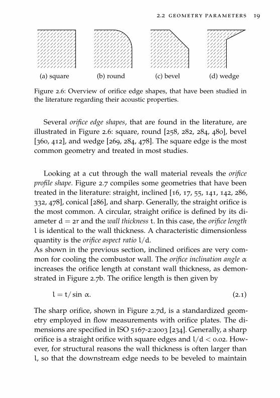
Several orifice edge shapes, that are found in the literature, areillustrated in Figure 2.6: square, round [258, 282, 284, 480], bevel[360, 412], and wedge [269, 284, 478]. The square edge is the mostcommon geometry and treated in most studies.
Looking at a cut through the wall material reveals the orificeprofile shape. Figure 2.7 compiles some geometries that have beentreated in the literature: straight, inclined [16, 17, 55, 141, 142, 286,332, 478], conical [286], and sharp. Generally, the straight orifice isthe most common. A circular, straight orifice is defined by its di-ameter d = 2r and the wall thickness t. In this case, the orifice lengthl is identical to the wall thickness. A characteristic dimensionlessquantity is the orifice aspect ratio l/d.As shown in the previous section, inclined orifices are very com-mon for cooling the combustor wall. The orifice inclination angle αincreases the orifice length at constant wall thickness, as demon-strated in Figure 2.7b. The orifice length is then given by
l = t/ sin α. (2.1)
The sharp orifice, shown in Figure 2.7d, is a standardized geom-etry employed in flow measurements with orifice plates. The di-mensions are specified in ISO 5167-2:2003 [234]. Generally, a sharporifice is a straight orifice with square edges and l/d < 0.02. How-ever, for structural reasons the wall thickness is often larger thanl, so that the downstream edge needs to be beveled to maintain

20 bias flow liners
draft – 2014.06.25 18:18 – claus lahiri
2r
t
(a) straight
draft – 2014.06.25 18:19 – claus lahiri
2r
t
l
αUg⇒(b) inclined
draft – 2014.06.17 16:03 – claus lahiri
t
(c) conical
draft – 2014.06.17 16:03 – claus lahiri
α
t l
⇓Ub
(d) sharp
Figure 2.7: Overview of orifice profile shapes, that have been studied inthe literature regarding their acoustic properties.
the sharp edge characteristics. According to the ISO standard, thebevel angle needs to be within 30° – 60°.
2.2.2 Perforation Geometry
Owing to their simplicity, single orifices are often employed in sci-entific studies. While many parameters can be investigated with asingle orifice, the arrangement of a multitude of orifices in a lineradds some more degrees of freedom and complexity. Figure 2.8illustrates different perforation patterns.
The most simple pattern is the square perforation pattern pre-sented in Figure 2.8a. Shown is the plan view of a segment ofa cylindrical liner with the coordinates x in axial direction and θin circumferential direction. Any curvature effects are neglectedfor now, so that the liner is considered to be flat. The orifices arearranged in straight rows in axial and circumferential direction.The perforation spacing s is identical in both directions, forming asquare grid. Based on the perforation spacing, an orifice unit areasx × sθ can be assigned to each orifice (in the case of the square
2.2 geometry parameters 21
x
θ
s
s
LLeff
Lc
(a) square
x
θ
sx
sθ
(b) rectangular
x
θ
sx
sθ
α
s ′x
(c) staggered
x
θ
Leff
(d) nonuniform
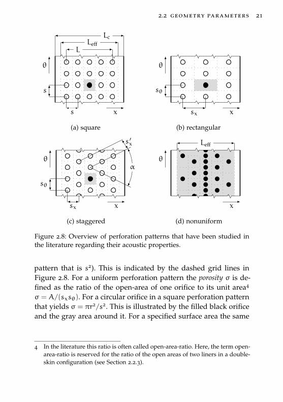
Figure 2.8: Overview of perforation patterns that have been studied inthe literature regarding their acoustic properties.
pattern that is s2). This is indicated by the dashed grid lines inFigure 2.8. For a uniform perforation pattern the porosity σ is de-fined as the ratio of the open-area of one orifice to its unit area4
σ = A/(sxsθ). For a circular orifice in a square perforation patternthat yields σ = πr2/s2. This is illustrated by the filled black orificeand the gray area around it. For a specified surface area the same
4 In the literature this ratio is often called open-area-ratio. Here, the term open-area-ratio is reserved for the ratio of the open areas of two liners in a double-skin configuration (see Section 2.2.3).
22 bias flow liners
porosity can be realized by applying many small orifices or fewerlarge ones.
The maximum axial distance between two orifices defines theperforation length L. An effective perforation length Leff of the perfo-ration can be specified according to the unit areas of all orifices.Finally, the cavity length Lc is defined by the dimensions of the cav-ity behind the liner. In a theoretically constructed setup the effec-tive perforation length and the cavity length would most probablybe identical (as they are in Figure 2.8b). In Figure 2.8a, the effec-tive perforation length is shorter than the cavity length, resultingin some margins on both sides. It is as well possible, that the ef-fective perforation length becomes longer than the cavity length,producing a ‘negative’ margin. In other cases the perforation onlycovers a fraction of the available length, resulting in large mar-gins of hard wall. Then, the perforation placement could be shiftedalong the axial coordinate. The default position is at the centerwith equal margins on both sides.
An important parameter regarding the efficiency of a bias flowliner is the total open area, which is the open area of all orificescombined. The larger the open area, the more mass flow is neededto achieve a certain bias flow velocity.
The rectangular perforation pattern in Figure 2.8b is similar to thesquare pattern described above. The only difference is that the ori-fice spacing is not identical in axial and circumferential direction.This can happen easily when designing a cylindrical liner of a cer-tain porosity. The selection of circumferential spacing is not con-tinuous, but dependent on the circular pitch resulting from thenumber of orifices around the circumference. The axial spacinghas to be adapted accordingly to obtain the desired porosity. Therectangular pattern is defined by the perforation aspect ratio sx/sθ.The influence of the aspect ratio on the acoustic performance wasstudied in [17, 288, 289].
The staggered perforation pattern in Figure 2.8c is the most wide-spread in technical applications. The structural strength of the ma-

2.2 geometry parameters 23
terial is enhanced compared to a rectangular or square pattern.Common perforation stagger angles α are 60° (sometimes calledtriangular pattern) and 45° (sometimes called diagonal pattern).At 60° the distances between any neighboring orifices are equalsθ = s ′x. Thus, the sheet material retains the most strength whileoffering the largest possible open area. The pattern presented herehas a stagger angle of 53.1°. This value might seem odd at first, butit can be easily obtained by just turning every second row of thesquare pattern about half the orifice circumferential spacing. Bydoing so, the porosity remains constant compared to the squarepattern, as in both cases sθ = sx. In order to obtain a 60° staggerangle the axial distance between the rows has to be reduced, sothat the porosity would be increased in relation to the square pat-tern.Another effect of the circumferential stagger is, that a potentialinteraction of two adjacent orifices in grazing flow direction is re-duced as their distance is doubled (the orifice in-between is movedsideways).
Figure 2.8d demonstrates an example of a nonuniform perfora-tion pattern. The term nonuniform is used for patterns where theporosity is not constant, either in axial direction (as shown), cir-cumferential direction, or both. Still, the pattern is not completelyrandom and shows some sort of regularity. In the example, the ‘lo-cal’ porosity increases towards the center of the liner. For nonuni-form patterns the porosity is given by the ratio of the total open-area to the area defined by the active length, as indicated in Fig-ure 2.8d. This gives an overall or average porosity. The significanceof this value might be questionable, but it provides a comparativevalue between uniform and nonuniform patterns. The influenceof nonuniform patterns is studied in [116, 259, 282] with very dif-ferent configurations.
24 bias flow liners
draft – 2014.06.17 16:04 – claus lahiri
sθ
s ′θ
αR
Figure 2.9: Effect of the curvature on the definition of the circumferentialperforation spacing.
Curvature
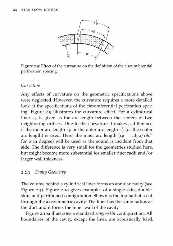
Any effects of curvature on the geometric specifications abovewere neglected. However, the curvature requires a more detailedlook at the specifications of the circumferential perforation spac-ing. Figure 2.9 illustrates the curvature effect. For a cylindricalliner sθ is given as the arc length between the centers of twoneighboring orifices. Due to the curvature it makes a differenceif the inner arc length sθ or the outer arc length s ′θ (or the centerarc length) is used. Here, the inner arc length (sθ = πRα/180◦
for α in degree) will be used as the sound is incident from thatside. The difference is very small for the geometries studied here,but might become more substantial for smaller duct radii and/orlarger wall thickness.
2.2.3 Cavity Geometry
The volume behind a cylindrical liner forms an annular cavity (seeFigure 2.4). Figure 2.10 gives examples of a single-skin, double-skin, and partitioned configuration. Shown is the top half of a cutthrough the axisymmetric cavity. The liner has the same radius asthe duct and it forms the inner wall of the cavity.
Figure 2.10a illustrates a standard single-skin configuration. Allboundaries of the cavity, except the liner, are acoustically hard.
2.2 geometry parameters 25
draft – 2014.06.26 14:20 – claus lahiri
R
Rc
Lc
(a) single-skin
draft – 2014.06.26 14:26 – claus lahiri
R1
R2
(b) double-skin
draft – 2014.06.26 14:29 – claus lahiri
Lc1 Lc2 Lc3
(c) partitioned
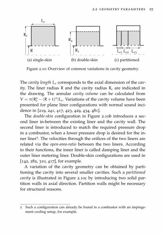
Figure 2.10: Overview of common variations in cavity geometry.
The cavity length Lc corresponds to the axial dimension of the cav-ity. The liner radius R and the cavity radius Rc are indicated inthe drawing. The annular cavity volume can be calculated fromV = π(R2
c − (R+ t)2)Lc. Variations of the cavity volume have beenpresented for plane liner configurations with normal sound inci-dence in [219, 241, 417, 423, 429, 434, 481].
The double-skin configuration in Figure 2.10b introduces a sec-ond liner in-between the existing liner and the cavity wall. Thesecond liner is introduced to match the required pressure dropin a combustor, when a lower pressure drop is desired for the in-ner liner5. The velocities through the orifices of the two liners arerelated via the open-area-ratio between the two liners. Accordingto their functions, the inner liner is called damping liner and theouter liner metering liner. Double-skin configurations are used in[142, 282, 310, 417], for example.
A variation of the cavity geometry can be obtained by parti-tioning the cavity into several smaller cavities. Such a partitionedcavity is illustrated in Figure 2.10c by introducing two solid par-tition walls in axial direction. Partition walls might be necessaryfor structural reasons.
5 Such a configuration can already be found in a combustor with an impinge-ment cooling setup, for example.
26 bias flow liners
2.3 thermodynamic parameters
A combustor operates at extreme pressure and temperature condi-tions. Many fluid properties change considerably when these twoparameters are changing. Appendix a.3 gives an overview of thebehavior of some properties of air with variation of pressure andtemperature.
2.3.1 Temperature
The temperature within the combustor is around 2000 K and thecooling flow is provided at temperatures between 500-800 K. Mostlaboratory test rigs for liner measurements operate at ambienttemperature, i. e. the temperature of the grazing flow and the biasflow is around 288 K. Some results are reported for tests includingcombustion [55, 294, 310, 357, 481, 484]. In that case, the tempera-ture is much higher, but it is fixed at that level so that the influenceof varying temperature on the absorption cannot be determined.Only a few studies exist where the temperature was controlled,e. g. involving perforated liners [381], a single orifice with cavity[144], or porous materials [93, 174, 355, 379, 381, 403, 462]. Mea-surements of porous materials at reduced temperature (172 K) arepresented in [9]. None of the references above include a bias flow.The only configuration where temperature effects have been stud-ied including a bias flow is a duct termination issuing a hot jet[104, 166, 251, 346, 370, 382].
Here, measurements are presented from the Hot Acoustic TestRig (see Section 6.6). It provides an acoustically defined environ-ment where the temperature of the grazing flow can be adjustedbetween ambient and 823 K. The bias flow is provided at a con-stant temperature of 288 K. The mean temperature of the grazingflow entering the lined section will serve as a reference tempera-ture.
2.4 acoustic parameters 27
2.3.2 Pressure
The combustor operates at very high static pressure levels. Com-monly, this is not accounted for when testing perforated liners.Even the measurements that involve combustion are typically atatmospheric conditions [55, 310, 481]. The Hot Acoustic Test Rigallows to increase the static pressure in the duct from ambientup to 1100 kPa (see Section 6.6), so that the influence of the staticpressure on the absorption can be determined.
2.4 acoustic parameters
2.4.1 Frequency
A combustion instability is a discrete frequency phenomena. How-ever, the exact frequency where the instability occurs cannot bepredicted and it changes with the operating condition of the com-bustor. Therefore, the frequency characteristic of the liner is oneof its most important features.
Commonly, the performance of a liner is measured over a rangeof frequencies. In order to obtain such a performance spectrum,various test signals can be applied, e. g. single-sine [52, 162, 247],multi-sine[82, 282], swept-sine [87], or broadband [90].
Closely related to the frequency, or more precisely the wavelength, is the spatial structure of the sound field. Due to the lowfrequency (< 1 kHz) nature of the combustion instabilities, it isoften the plane wave mode6 that is dominant [305]. Thus, moststudies are limited to plane waves. Some theoretical studies areavailable that describe the interaction of higher order modes withan acoustic liner, e. g. [140, 393].
6 That means, the acoustic field quantities are a function of the axial coordinateonly (see Section 5.3).
28 bias flow liners
2.4.2 Amplitude / Sound Pressure Level
The influence of the amplitude on the acoustic properties of anorifice has been the subject of many studies, e. g. [26, 58, 61, 72,105, 123, 225, 227, 228, 243, 327, 361, 441, 473, 474, 505]. Dependingon the amplitude, a linear or a nonlinear behavior is observed. Thedefinition of a linear system is given by Bendat and Piersol [47]:The response characteristics are additive7 and homogeneous8. Athigh amplitudes the behavior of the orifice is not homogeneousanymore, i. e. the response depends on the excitation amplitude.As a conclusion, the knowledge of the exact amplitude is ratherunimportant in the linear regime, while it becomes relevant in thenonlinear regime.
Unfortunately, the definition of the amplitude is not quite con-sistent in the literature. Actually, often no clear definition is given.Authors refer to: the particle velocity amplitude in the orifice [227,441], the pressure amplitude at the liner surface [41, 158, 161, 243],the amplitude of the incident wave [8, 415, 425], the amplitude ata fixed reference location in the hard-walled duct section in frontof the liner [82, 142, 199, 247], the peak amplitude of the standingwave field in the hard-wall duct section [327], the amplitude in theloudspeaker mounting [7], or the amplitude in the cavity behindthe perforation [227, 481].
It is generally assumed that the physical quantity relevant to thenonlinear behavior is the particle velocity in the orifice. However,in most cases it would take a great effort to measure the particlevelocity in the orifice, so that the amplitude is often given in termsof sound pressure level (SPL). Now, the three most common ap-proaches are discussed and evaluated for their comparability andpracticality.
7 Additive means, that the output to a sum of inputs is equal to the sum of theoutputs produced by each input individually: f(x1 + x2) = f(x1) + f(x2) [47].
8 Homogeneous means, that the output produced by a constant times the inputis equal to the constant times the output produced by the input alone: f(cx) =cf(x) [47].
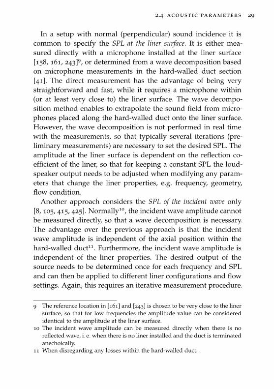
2.4 acoustic parameters 29
In a setup with normal (perpendicular) sound incidence it iscommon to specify the SPL at the liner surface. It is either mea-sured directly with a microphone installed at the liner surface[158, 161, 243]9, or determined from a wave decomposition basedon microphone measurements in the hard-walled duct section[41]. The direct measurement has the advantage of being verystraightforward and fast, while it requires a microphone within(or at least very close to) the liner surface. The wave decompo-sition method enables to extrapolate the sound field from micro-phones placed along the hard-walled duct onto the liner surface.However, the wave decomposition is not performed in real timewith the measurements, so that typically several iterations (pre-liminary measurements) are necessary to set the desired SPL. Theamplitude at the liner surface is dependent on the reflection co-efficient of the liner, so that for keeping a constant SPL the loud-speaker output needs to be adjusted when modifying any param-eters that change the liner properties, e.g. frequency, geometry,flow condition.
Another approach considers the SPL of the incident wave only[8, 105, 415, 425]. Normally10, the incident wave amplitude cannotbe measured directly, so that a wave decomposition is necessary.The advantage over the previous approach is that the incidentwave amplitude is independent of the axial position within thehard-walled duct11. Furthermore, the incident wave amplitude isindependent of the liner properties. The desired output of thesource needs to be determined once for each frequency and SPLand can then be applied to different liner configurations and flowsettings. Again, this requires an iterative measurement procedure.
9 The reference location in [161] and [243] is chosen to be very close to the linersurface, so that for low frequencies the amplitude value can be consideredidentical to the amplitude at the liner surface.
10 The incident wave amplitude can be measured directly when there is noreflected wave, i. e. when there is no liner installed and the duct is terminatedanechoically.
11 When disregarding any losses within the hard-walled duct.
30 bias flow liners
small R
large R
Liner654Microphone 3
xref 0
105
115
125
Axial Coordinate
SPL
indB
|p′||p+|
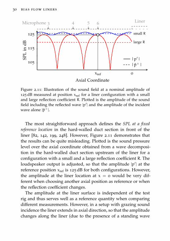
Figure 2.11: Illustration of the sound field at a nominal amplitude of125 dB measured at position xref for a liner configuration with a smalland large reflection coefficient R. Plotted is the amplitude of the soundfield including the reflected wave |p′| and the amplitude of the incidentwave alone |p+|.
The most straightforward approach defines the SPL at a fixedreference location in the hard-walled duct section in front of theliner [82, 142, 199, 248]. However, Figure 2.11 demonstrates thatthe results can be quite misleading. Plotted is the sound pressurelevel over the axial coordinate obtained from a wave decomposi-tion in the hard-walled duct section upstream of the liner for aconfiguration with a small and a large reflection coefficient R. Theloudspeaker output is adjusted, so that the amplitude |p′| at thereference position xref is 125 dB for both configurations. However,the amplitude at the liner location at x = 0 would be very dif-ferent when choosing another axial position as reference or whenthe reflection coefficient changes.
The amplitude at the liner surface is independent of the testrig and thus serves well as a reference quantity when comparingdifferent measurements. However, in a setup with grazing soundincidence the liner extends in axial direction, so that the amplitudechanges along the liner (due to the presence of a standing wave
2.4 acoustic parameters 31
content in the sound field and due to the absorption of the liner).In this case, it is difficult to choose the ’correct’ reference plane,so this approach is not applicable in a grazing incidence setup.The incident wave amplitude should be the preferred quantity ina grazing incidence setup.
Multi-Sine Signals
2 6 10-2
-1
0
1
2
Time in ms
p′
inPa
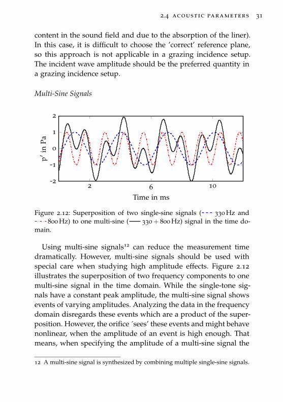
Figure 2.12: Superposition of two single-sine signals ( 330 Hz and800 Hz) to one multi-sine ( 330 + 800 Hz) signal in the time do-
main.
Using multi-sine signals12 can reduce the measurement timedramatically. However, multi-sine signals should be used withspecial care when studying high amplitude effects. Figure 2.12illustrates the superposition of two frequency components to onemulti-sine signal in the time domain. While the single-tone sig-nals have a constant peak amplitude, the multi-sine signal showsevents of varying amplitudes. Analyzing the data in the frequencydomain disregards these events which are a product of the super-position. However, the orifice ´sees’ these events and might behavenonlinear, when the amplitude of an event is high enough. Thatmeans, when specifying the amplitude of a multi-sine signal the
12 A multi-sine signal is synthesized by combining multiple single-sine signals.
32 bias flow liners
overall SPL is the more appropriate quantity, and not the SPL ofeach tonal component separately. In other words, in order to en-sure that one acts in the linear domain the overall SPL should beconsulted. For a single-sine signal the amplitude of the tone andthe overall SPL are identical.
Another characteristic of multi-sine signals in the nonlinear do-main is that the different frequency components might influenceeach other [68, 281].
2.5 flow parameters
The flow paths in a combustor liner were discussed in Section 2.1.The general motion of fluid at the liner is a combination of a flowgrazing the liner surface tangentially on the inside of the combus-tor, referred to as grazing flow, and the cooling flow through theorifices of the liner, referred to as bias flow.
2.5.1 Grazing Flow
The effect of a grazing flow on the acoustic properties of orificesand liners has been studied in many publications, e. g. [21, 24,56, 81, 83, 106, 122, 145, 153–155, 175, 177, 209, 215, 244, 264–266,268, 274, 290, 312, 322, 329, 341, 364, 384, 396, 406, 426, 467, 478,480]. This interest in the grazing flow effect is mostly motivatedby the application of liners in aero engine inlets and bypass ducts,where grazing flow Mach numbers of 0.5-0.7 are typical. This is incontrast to gas turbine combustors where Mg = 0.05 is a commonvalue. So the typical grazing flow Mach number is an order ofmagnitude lower. Most of the references given above study theinfluence of the flow boundary layer on the acoustic behavior, i. e.the significance of the friction velocity over the mean flow velocity.However, Peat et al. [364] conclude that the mean flow velocityis the adequate parameter when the flow is turbulent and fullydeveloped. The flow in a combustion chamber as well as in the
2.5 flow parameters 33
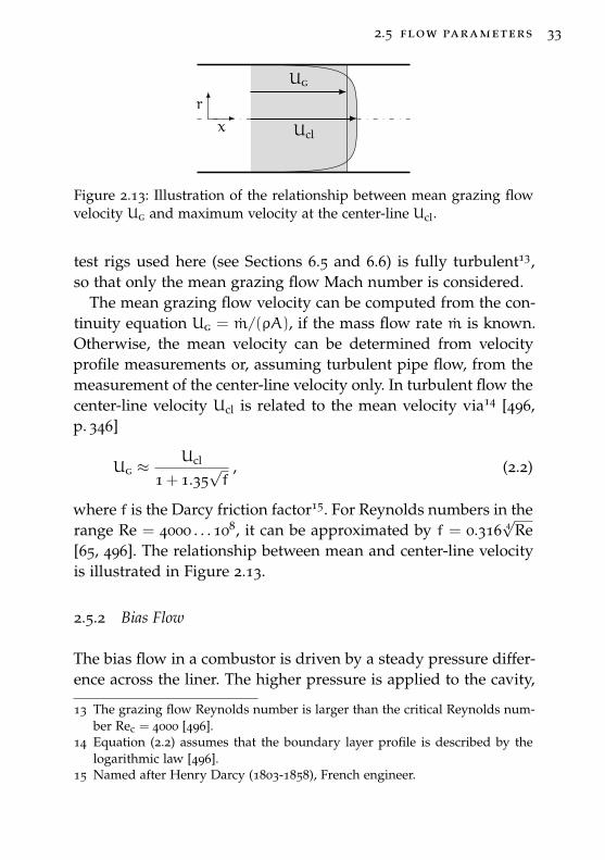
draft – 2014.06.30 15:36 – claus lahiri
Ug
Uclx
r
Figure 2.13: Illustration of the relationship between mean grazing flowvelocity Ug and maximum velocity at the center-line Ucl.
test rigs used here (see Sections 6.5 and 6.6) is fully turbulent13,so that only the mean grazing flow Mach number is considered.
The mean grazing flow velocity can be computed from the con-tinuity equation Ug = m/(ρA), if the mass flow rate m is known.Otherwise, the mean velocity can be determined from velocityprofile measurements or, assuming turbulent pipe flow, from themeasurement of the center-line velocity only. In turbulent flow thecenter-line velocity Ucl is related to the mean velocity via14 [496,p. 346]
Ug ≈Ucl
1 + 1.35√f
, (2.2)
where f is the Darcy friction factor15. For Reynolds numbers in therange Re = 4000 . . . 108, it can be approximated by f = 0.316 4
√Re
[65, 496]. The relationship between mean and center-line velocityis illustrated in Figure 2.13.
2.5.2 Bias Flow
The bias flow in a combustor is driven by a steady pressure differ-ence across the liner. The higher pressure is applied to the cavity,
13 The grazing flow Reynolds number is larger than the critical Reynolds num-ber Rec = 4000 [496].
14 Equation (2.2) assumes that the boundary layer profile is described by thelogarithmic law [496].
15 Named after Henry Darcy (1803-1858), French engineer.
34 bias flow liners
so that the fluid discharges from the cavity, through the orifices,into the combustor. Some authors have studied the effect of neg-ative bias flow [6, 26, 87, 241, 276, 332]16, that is in the oppositedirection as described above. However, such a concept cannot beapplied to a combustion chamber. The discharging hot gas wouldcompromise the integrity of the liner and other components down-stream. Therefore, this study exclusively treats bias flow directedinto the combustor or test duct. The effect of a periodic oscillating,unsteady bias flow is studied by Heuwinkel et al. [200] and Lahiriet al. [280, 281] and also, will not be included here.
A steady bias flow can be defined by its mass flow rate, thepressure drop across the wall, or the velocity through the orifices.As these three quantities provide different information and enabledifferent conclusions it is an advantage to have all three availableat the same time.
The bias flow pressure drop, that is the pressure difference acrossthe liner, is an operational quantity of a gas turbine combustor. Acertain operating condition yields a fixed pressure drop. The airflow in the combustor is regulated by the relation of the pressuredrops of the different components. Thus, it is very important tomatch the pressure drop when replacing a liner with a new de-sign. Otherwise the intended air distribution might change. Thepressure drop across the liner can be measured with a differentialpressure meter via static pressure taps on both sides of the liner,i. e. in the cavity and in the duct. The pressure drop is then givenin relation to the absolute pressure in the duct as
∆P =pcavity − pduct
pduct× 100 % . (2.3)
In a double-skin configuration (see Section 2.2.3) the pressuredrop refers to the total pressure drop across both liners, as this
16 Jing and Sun [241] and von Barthel [26] found that blowing and suctionhave the same effect. However, when a grazing flow is present the resultsare substantially different [332], e. g. Tonon et al. [478] report that the acous-tic resistance appears to be a factor four lower for a grazing-bias outflowcompared to a grazing-bias inflow case.
2.5 flow parameters 35
is the relevant quantity for the operation of the combustor. A typ-ical pressure drop across a combustor wall is about 3 % [417].
The bias flow mass flow rate can be a measure of the efficiency ofthe liner, i. e. a liner achieving the same damping performance at alower mass flow rate is more efficient. The efficiency is evaluatedfor the liner as a whole, so that the total mass flow rate, insteadof the mass flow rate per orifice, should be compared. Most lab-oratory experiments use a mass flow controller to adjust the biasflow. Thus, its value is available in most cases.
The bias flow velocity is the quantity that is related to the absorp-tion of sound. Typically, the velocity is not measured directly, butestimated from the pressure difference across the liner or the massflow rate through the liner.
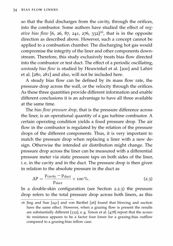
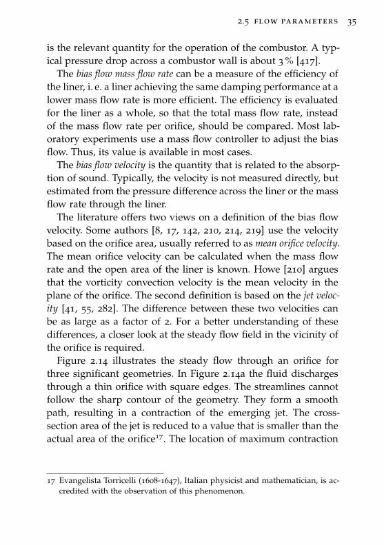
The literature offers two views on a definition of the bias flowvelocity. Some authors [8, 17, 142, 210, 214, 219] use the velocitybased on the orifice area, usually referred to as mean orifice velocity.The mean orifice velocity can be calculated when the mass flowrate and the open area of the liner is known. Howe [210] arguesthat the vorticity convection velocity is the mean velocity in theplane of the orifice. The second definition is based on the jet veloc-ity [41, 55, 282]. The difference between these two velocities canbe as large as a factor of 2. For a better understanding of thesedifferences, a closer look at the steady flow field in the vicinity ofthe orifice is required.
Figure 2.14 illustrates the steady flow through an orifice forthree significant geometries. In Figure 2.14a the fluid dischargesthrough a thin orifice with square edges. The streamlines cannotfollow the sharp contour of the geometry. They form a smoothpath, resulting in a contraction of the emerging jet. The cross-section area of the jet is reduced to a value that is smaller than theactual area of the orifice17. The location of maximum contraction
17 Evangelista Torricelli (1608-1647), Italian physicist and mathematician, is ac-credited with the observation of this phenomenon.
36 bias flow liners
draft – 2014.06.27 12:59 – claus lahiri
1
2
venacontracta
(a) thin orifice
draft – 2014.06.27 12:59 – claus lahiri
12
(b) thick orifice
draft – 2014.06.27 12:59 – claus lahiri
1
2
(c) round edge
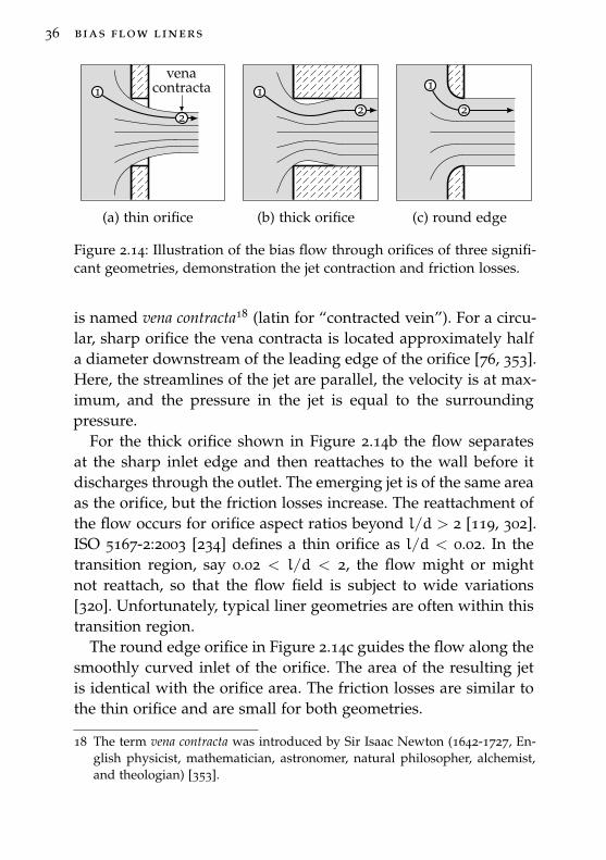
Figure 2.14: Illustration of the bias flow through orifices of three signifi-cant geometries, demonstration the jet contraction and friction losses.
is named vena contracta18 (latin for “contracted vein”). For a circu-lar, sharp orifice the vena contracta is located approximately halfa diameter downstream of the leading edge of the orifice [76, 353].Here, the streamlines of the jet are parallel, the velocity is at max-imum, and the pressure in the jet is equal to the surroundingpressure.
For the thick orifice shown in Figure 2.14b the flow separatesat the sharp inlet edge and then reattaches to the wall before itdischarges through the outlet. The emerging jet is of the same areaas the orifice, but the friction losses increase. The reattachment ofthe flow occurs for orifice aspect ratios beyond l/d > 2 [119, 302].ISO 5167-2:2003 [234] defines a thin orifice as l/d < 0.02. In thetransition region, say 0.02 < l/d < 2, the flow might or mightnot reattach, so that the flow field is subject to wide variations[320]. Unfortunately, typical liner geometries are often within thistransition region.
The round edge orifice in Figure 2.14c guides the flow along thesmoothly curved inlet of the orifice. The area of the resulting jetis identical with the orifice area. The friction losses are similar tothe thin orifice and are small for both geometries.
18 The term vena contracta was introduced by Sir Isaac Newton (1642-1727, En-glish physicist, mathematician, astronomer, natural philosopher, alchemist,and theologian) [353].
2.5 flow parameters 37
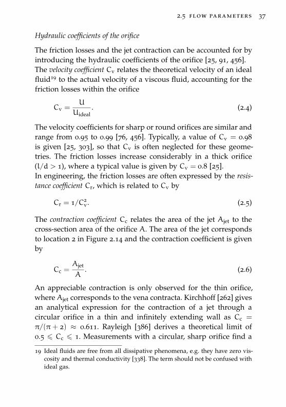
Hydraulic coefficients of the orifice
The friction losses and the jet contraction can be accounted for byintroducing the hydraulic coefficients of the orifice [25, 91, 456].The velocity coefficient Cv relates the theoretical velocity of an idealfluid19 to the actual velocity of a viscous fluid, accounting for thefriction losses within the orifice
Cv =U
Uideal. (2.4)
The velocity coefficients for sharp or round orifices are similar andrange from 0.95 to 0.99 [76, 456]. Typically, a value of Cv = 0.98is given [25, 303], so that Cv is often neglected for these geome-tries. The friction losses increase considerably in a thick orifice(l/d > 1), where a typical value is given by Cv = 0.8 [25].In engineering, the friction losses are often expressed by the resis-tance coefficient Cr, which is related to Cv by
Cr = 1/C2v. (2.5)
The contraction coefficient Cc relates the area of the jet Ajet to thecross-section area of the orifice A. The area of the jet correspondsto location 2 in Figure 2.14 and the contraction coefficient is givenby
Cc =Ajet
A. (2.6)
An appreciable contraction is only observed for the thin orifice,where Ajet corresponds to the vena contracta. Kirchhoff [262] givesan analytical expression for the contraction of a jet through acircular orifice in a thin and infinitely extending wall as Cc =
π/(π + 2) ≈ 0.611. Rayleigh [386] derives a theoretical limit of0.5 6 Cc 6 1. Measurements with a circular, sharp orifice find a
19 Ideal fluids are free from all dissipative phenomena, e.g. they have zero vis-cosity and thermal conductivity [338]. The term should not be confused withideal gas.
38 bias flow liners
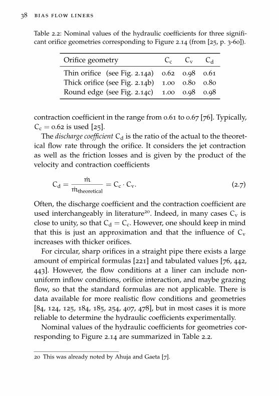
Table 2.2: Nominal values of the hydraulic coefficients for three signifi-cant orifice geometries corresponding to Figure 2.14 (from [25, p. 3-60]).
Orifice geometry Cc Cv Cd
Thin orifice (see Fig. 2.14a) 0.62 0.98 0.61Thick orifice (see Fig. 2.14b) 1.00 0.80 0.80Round edge (see Fig. 2.14c) 1.00 0.98 0.98
contraction coefficient in the range from 0.61 to 0.67 [76]. Typically,Cc = 0.62 is used [25].
The discharge coefficient Cd is the ratio of the actual to the theoret-ical flow rate through the orifice. It considers the jet contractionas well as the friction losses and is given by the product of thevelocity and contraction coefficients
Cd =m
mtheoretical= Cc ·Cv. (2.7)
Often, the discharge coefficient and the contraction coefficient areused interchangeably in literature20. Indeed, in many cases Cv isclose to unity, so that Cd = Cc. However, one should keep in mindthat this is just an approximation and that the influence of Cv
increases with thicker orifices.For circular, sharp orifices in a straight pipe there exists a large
amount of empirical formulas [221] and tabulated values [76, 442,443]. However, the flow conditions at a liner can include non-uniform inflow conditions, orifice interaction, and maybe grazingflow, so that the standard formulas are not applicable. There isdata available for more realistic flow conditions and geometries[84, 124, 125, 184, 185, 254, 407, 478], but in most cases it is morereliable to determine the hydraulic coefficients experimentally.
Nominal values of the hydraulic coefficients for geometries cor-responding to Figure 2.14 are summarized in Table 2.2.
20 This was already noted by Ahuja and Gaeta [7].
2.5 flow parameters 39
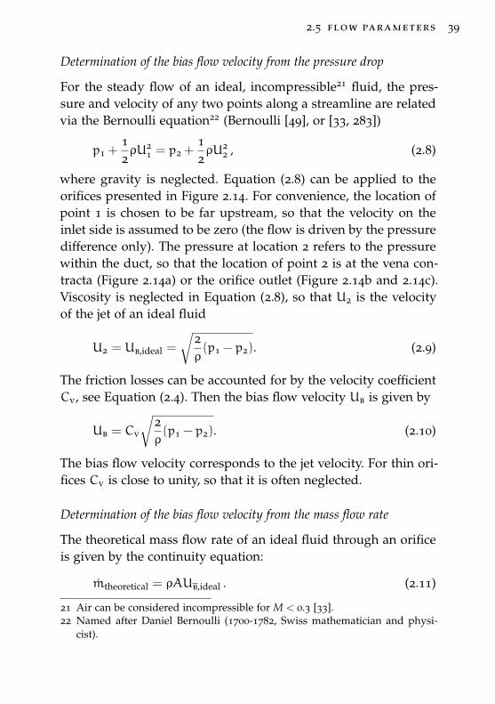
Determination of the bias flow velocity from the pressure drop
For the steady flow of an ideal, incompressible21 fluid, the pres-sure and velocity of any two points along a streamline are relatedvia the Bernoulli equation22 (Bernoulli [49], or [33, 283])
p1 +12ρU2
1 = p2 +12ρU2
2 , (2.8)
where gravity is neglected. Equation (2.8) can be applied to theorifices presented in Figure 2.14. For convenience, the location ofpoint 1 is chosen to be far upstream, so that the velocity on theinlet side is assumed to be zero (the flow is driven by the pressuredifference only). The pressure at location 2 refers to the pressurewithin the duct, so that the location of point 2 is at the vena con-tracta (Figure 2.14a) or the orifice outlet (Figure 2.14b and 2.14c).Viscosity is neglected in Equation (2.8), so that U2 is the velocityof the jet of an ideal fluid
U2 = Ub,ideal =
√2ρ(p1 − p2). (2.9)
The friction losses can be accounted for by the velocity coefficientCv, see Equation (2.4). Then the bias flow velocity Ub is given by
Ub = Cv
√2ρ(p1 − p2). (2.10)
The bias flow velocity corresponds to the jet velocity. For thin ori-fices Cv is close to unity, so that it is often neglected.
Determination of the bias flow velocity from the mass flow rate
The theoretical mass flow rate of an ideal fluid through an orificeis given by the continuity equation:
mtheoretical = ρAUb,ideal . (2.11)
21 Air can be considered incompressible for M < 0.3 [33].22 Named after Daniel Bernoulli (1700-1782, Swiss mathematician and physi-
cist).
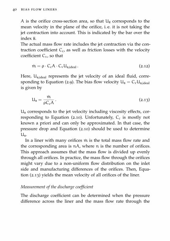
40 bias flow liners
A is the orifice cross-section area, so that Ub corresponds to themean velocity in the plane of the orifice, i. e. it is not taking thejet contraction into account. This is indicated by the bar over theindex b.The actual mass flow rate includes the jet contraction via the con-traction coefficient Cc, as well as friction losses with the velocitycoefficient Cv, so that
m = ρ ·CcA ·CvUb,ideal . (2.12)
Here, Ub,ideal represents the jet velocity of an ideal fluid, corre-sponding to Equation (2.9). The bias flow velocity Ub = CvUb,ideal
is given by
Ub =m
ρCcA. (2.13)
Ub corresponds to the jet velocity including viscosity effects, cor-responding to Equation (2.10). Unfortunately, Cc is mostly notknown a priori and can only be approximated. In that case, thepressure drop and Equation (2.10) should be used to determineUb.
In a liner with many orifices m is the total mass flow rate andthe corresponding area is nA, where n is the number of orifices.This approach assumes that the mass flow is divided up evenlythrough all orifices. In practice, the mass flow through the orificesmight vary due to a non-uniform flow distribution on the inletside and manufacturing differences of the orifices. Then, Equa-tion (2.13) yields the mean velocity of all orifices of the liner.
Measurement of the discharge coefficient
The discharge coefficient can be determined when the pressuredifference across the liner and the mass flow rate through the
2.5 flow parameters 41
liner are both available. Combining Equations (2.10) and (2.13),together with (2.7) yields
Cd =m
ρA√
2ρ(p1 − p2)
. (2.14)
For sufficiently thin orifices it can be assumed that Cv is close tounity, so that Cd ≈ Cc.
Here, the bias flow velocity refers to the velocity of the jet asdefined in Equations (2.10) and (2.13). A certain mass flow rate orpressure difference is set for the measurement, while both quanti-ties are recorded. Then, the velocity is calculated from the pres-sure difference with Equation (2.10), where it is assumed thatCv = 1. The bias flow velocity is given in dimensionless formas the bias flow Mach number
Mb =Ub
c(2.15)
Furthermore, Cd is calculated from the mass flow rate and thepressure difference with Equation (2.13).

3L I T E R AT U R E O N B I A S F L O W L I N E R S
Historically, the damping effect of a bias flow orifice was observedin 1916, when Borth [73] reports on the successful suppression ofresonances in the ducts of a piston blower with the help of a biasflow orifice. In fact, he created a constriction by partially closing athrottle valve. His observation was confirmed by Maier and Lutz[311] and Lutz [309], who eliminated resonances by deliberatelyplacing orifice plates into the exhaust ducts of combustion enginesand reciprocating engines, respectively.
3.1 bias flow as a concept of impedance control
The first study of a more fundamental nature was published in1950 by McAuliffe [319], presenting the results of impedance tubemeasurements. He demonstrated the dependency of the orificeimpedance on a steady bias flow. Increasing the velocity revealeda substantial drop of the orifice reactance and a linear increaseof the orifice resistance1. When applied to a Helmholtz resonator,the bias flow provokes a shift of the resonance frequency to highervalues and a decrease of the Q factor2 of the resonance. Other au-
1 The resistance and the reactance are, respectively, the real and imaginarypart of the acoustic impedance, which will be introduced in Section 4.2.
2 The Q factor, short for quality factor, describes the bandwidth of a resonance.A high Q factor represents a sharp peak, while a resonance with a low Q hasa higher bandwidth.
44 literature on bias flow liners
thors reproduced these findings with a wide variety of differentsetups: The same setup was used by Westervelt [491], the experi-ments of Barthel [26] were performed with a Helmholtz resonatorwith normal sound incidence, the theoretical setup of Ingard [226]consisted of a perforated screen, Mechel et al. [326] studied a ducttermination, and Mechel et al. [325] employed screens of porousmaterials. In conclusion of these studies, Utvik et al. [483, p. 3]summarize the general effects of the flow: “Alteration in absorp-tion, which can either increase or decrease the damping effective-ness of the liner configuration; and a shift in resonant frequency,with broadening of the bandwidth characteristics.”
In the meantime, technological advancements have producedfurther applications of the bias flow concept, namely the suppres-sion of combustion instabilities in rocket engines [20, 62, 78, 170,180, 300, 367, 368, 484]. An early patent describes, “[. . . ] a combus-tion chamber with a perforated absorption liner having a regula-tor [. . . ] to control the air flow in the space behind the liner andthrough the perforations thereof in such a manner so as to com-pensate for variations in the absorption of the liner with variationsin pressure level” (US2941356 [62, p. 1]).
Feder and Dean [158] and Dean and Tester [118] propose thebias flow concept as a method of impedance control to turbofaninlet liners. Dean and Tester [118] see the greatest benefit in theability to easily tune the impedance of the liner when it is installedin an engine. This helps to overcome the inaccuracies of the avail-able models, thus reducing the need for expensive trial-and-errortesting.
The effect of the bias flow is commonly modeled by a resistancethat depends linearly on the bias flow velocity. Several authors[118, 171, 227, 326, 459, 491] use this approach with varying em-pirical constants. While an effect on the reactance has also beenreported, this is often not reflected in the models.The impact of the bias flow on the impedance characteristics isvery similar to the behavior observed at high amplitude excita-
3.2 sound absorption due to vorticity shedding 45
tion [26, 58, 61, 72, 105, 123, 225, 227, 228, 243, 327, 361, 441, 473,474, 505]. Indeed, the high amplitude produces an oscillating flowthrough the orifice [228, 423, 473], so that the relevant quantityin both cases is the velocity in the orifice. Dean and Tester [118]include the bias flow in their impedance model by simply replac-ing the acoustic particle velocity v′ with the bias flow velocity Ub.However, this can only be correct if Ub � |v′|.
The impedance model of Bauer [34] is often referred to whenperforations with bias flow are involved, e. g. [14, 18, 143]. Actu-ally, Bauer’s model includes only a v′ term describing the nonlin-earity at high amplitudes, but not an explicit bias flow term. How-ever, it seems common practice to replace the acoustic velocity inthe nonlinear term with the bias flow velocity, as Dean and Tester[118] demonstrated. The Bauer model is presented in Section 4.6.
After a long break, the bias flow concept was revived in a com-prehensive study initiated by the Boeing Company [56, 57]. Thework regarding the bias flow involves measurements of variousliner geometries as well as impedance modeling [52–54, 161, 162,276, 373]. The resulting impedance model proposed by Betts [52,54] is based on the state of the art models used in the industrywith the addition of a bias flow resistance term. The bias flowterm is integrated in the nonlinear impedance term by using thesum of the acoustic particle velocity and bias flow velocity as pro-posed by Premo [373]. The impedance model will be referred toas Betts model and is discussed in more detail in Section 4.7.
3.2 sound absorption due to vorticity shedding
In the late 1970s Bechert et al. [39, 40] could provide some insightinto the interaction of sound with a turbulent jet. In their experi-ments they observed a substantial attenuation at low frequenciesfor pure tone sound propagating through a nozzle along a tur-bulent jet. The conical nozzle issuing the jet was located in ananechoic room, while the acoustic signal was introduced into the
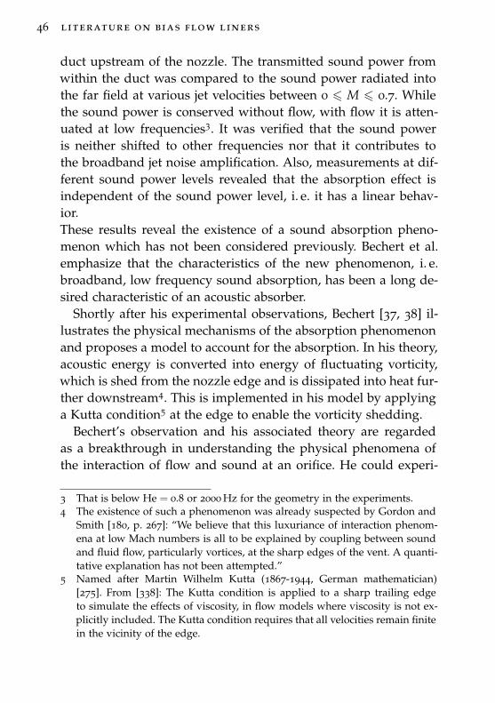
46 literature on bias flow liners
duct upstream of the nozzle. The transmitted sound power fromwithin the duct was compared to the sound power radiated intothe far field at various jet velocities between 0 6 M 6 0.7. Whilethe sound power is conserved without flow, with flow it is atten-uated at low frequencies3. It was verified that the sound poweris neither shifted to other frequencies nor that it contributes tothe broadband jet noise amplification. Also, measurements at dif-ferent sound power levels revealed that the absorption effect isindependent of the sound power level, i. e. it has a linear behav-ior.These results reveal the existence of a sound absorption pheno-menon which has not been considered previously. Bechert et al.emphasize that the characteristics of the new phenomenon, i. e.broadband, low frequency sound absorption, has been a long de-sired characteristic of an acoustic absorber.
Shortly after his experimental observations, Bechert [37, 38] il-lustrates the physical mechanisms of the absorption phenomenonand proposes a model to account for the absorption. In his theory,acoustic energy is converted into energy of fluctuating vorticity,which is shed from the nozzle edge and is dissipated into heat fur-ther downstream4. This is implemented in his model by applyinga Kutta condition5 at the edge to enable the vorticity shedding.
Bechert’s observation and his associated theory are regardedas a breakthrough in understanding the physical phenomena ofthe interaction of flow and sound at an orifice. He could experi-
3 That is below He = 0.8 or 2000 Hz for the geometry in the experiments.4 The existence of such a phenomenon was already suspected by Gordon and
Smith [180, p. 267]: “We believe that this luxuriance of interaction phenom-ena at low Mach numbers is all to be explained by coupling between soundand fluid flow, particularly vortices, at the sharp edges of the vent. A quanti-tative explanation has not been attempted.”
5 Named after Martin Wilhelm Kutta (1867-1944, German mathematician)[275]. From [338]: The Kutta condition is applied to a sharp trailing edgeto simulate the effects of viscosity, in flow models where viscosity is not ex-plicitly included. The Kutta condition requires that all velocities remain finitein the vicinity of the edge.
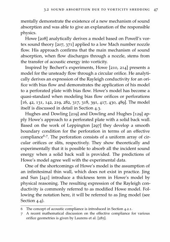
3.2 sound absorption due to vorticity shedding 47
mentally demonstrate the existence of a new mechanism of soundabsorption and was able to give an explanation of the responsiblephysics.
Howe [208] analytically derives a model based on Powell’s vor-tex sound theory [207, 371] applied to a low Mach number nozzleflow. His approach confirms that the main mechanism of soundabsorption, when flow discharges through a nozzle, stems fromthe transfer of acoustic energy into vorticity.
Inspired by Bechert’s experiments, Howe [210, 214] presents amodel for the unsteady flow through a circular orifice. He analyti-cally derives an expression of the Rayleigh conductivity for an ori-fice with bias flow and demonstrates the application of his modelto a perforated plate with bias flow. Howe’s model has become aquasi-standard when modeling bias flow orifices or perforations[16, 42, 131, 142, 219, 282, 317, 318, 391, 417, 430, 489]. The modelitself is discussed in detail in Section 4.3.
Hughes and Dowling [219] and Dowling and Hughes [129] ap-ply Howe’s approach to a perforated plate with a solid back wall.Based on the work of Leppington [297] they develop a smoothboundary condition for the perforation in terms of an effectivecompliance6,7. The perforation consists of a uniform array of cir-cular orifices or slits, respectively. They show theoretically andexperimentally that it is possible to absorb all the incident soundenergy when a solid back wall is provided. The predictions ofHowe’s model agree well with the experimental data.
One of the shortcomings of Howe’s model is the assumption ofan infinitesimal thin wall, which does not exist in practice. Jingand Sun [241] introduce a thickness term in Howe’s model byphysical reasoning. The resulting expression of the Rayleigh con-ductivity is commonly referred to as modified Howe model. Fol-lowing the notation here, it will be referred to as Jing model (seeSection 4.4).
6 The concept of acoustic compliance is introduced in Section 4.2.1.7 A recent mathematical discussion on the effective compliance for various
orifice geometries is given by Laurens et al. [285].
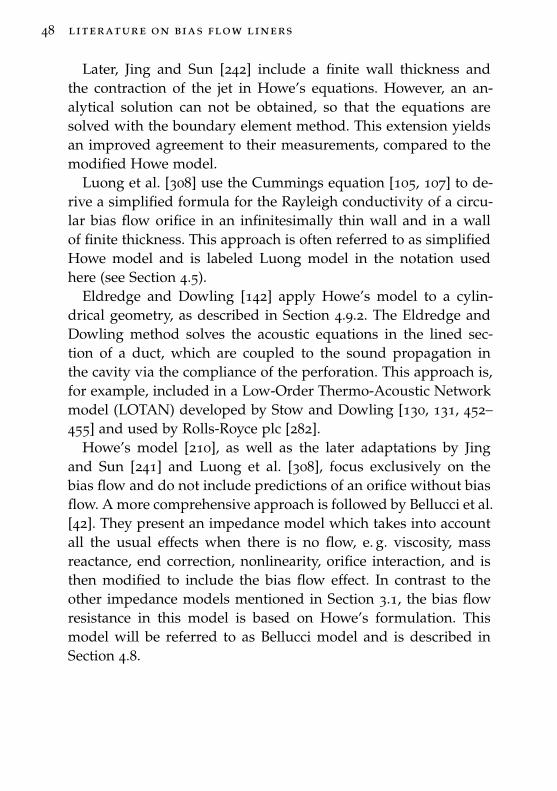
48 literature on bias flow liners
Later, Jing and Sun [242] include a finite wall thickness andthe contraction of the jet in Howe’s equations. However, an an-alytical solution can not be obtained, so that the equations aresolved with the boundary element method. This extension yieldsan improved agreement to their measurements, compared to themodified Howe model.
Luong et al. [308] use the Cummings equation [105, 107] to de-rive a simplified formula for the Rayleigh conductivity of a circu-lar bias flow orifice in an infinitesimally thin wall and in a wallof finite thickness. This approach is often referred to as simplifiedHowe model and is labeled Luong model in the notation usedhere (see Section 4.5).
Eldredge and Dowling [142] apply Howe’s model to a cylin-drical geometry, as described in Section 4.9.2. The Eldredge andDowling method solves the acoustic equations in the lined sec-tion of a duct, which are coupled to the sound propagation inthe cavity via the compliance of the perforation. This approach is,for example, included in a Low-Order Thermo-Acoustic Networkmodel (LOTAN) developed by Stow and Dowling [130, 131, 452–455] and used by Rolls-Royce plc [282].
Howe’s model [210], as well as the later adaptations by Jingand Sun [241] and Luong et al. [308], focus exclusively on thebias flow and do not include predictions of an orifice without biasflow. A more comprehensive approach is followed by Bellucci et al.[42]. They present an impedance model which takes into accountall the usual effects when there is no flow, e. g. viscosity, massreactance, end correction, nonlinearity, orifice interaction, and isthen modified to include the bias flow effect. In contrast to theother impedance models mentioned in Section 3.1, the bias flowresistance in this model is based on Howe’s formulation. Thismodel will be referred to as Bellucci model and is described inSection 4.8.
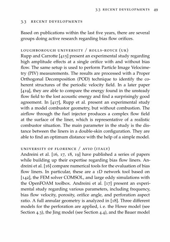
3.3 recent developments 49
3.3 recent developments
Based on publications within the last five years, there are severalgroups doing active research regarding bias flow orifices.
loughborough university / rolls-royce (uk)Rupp and Carrotte [415] present an experimental study regardinghigh amplitude effects at a single orifice with and without biasflow. The same setup is used to perform Particle Image Velocime-try (PIV) measurements. The results are processed with a ProperOrthogonal Decomposition (POD) technique to identify the co-herent structures of the periodic velocity field. In a later paper[419], they are able to compare the energy found in the unsteadyflow field to the lost acoustic energy and find a surprisingly goodagreement. In [417], Rupp et al. present an experimental studywith a model combustor geometry, but without combustion. Theairflow through the fuel injector produces a complex flow fieldat the surface of the liner, which is representative of a realisticcombustor situation. The main parameter in the study is the dis-tance between the liners in a double-skin configuration. They areable to find an optimum distance with the help of a simple model.
university of florence / avio (italy)Andreini et al. [16, 17, 18, 19] have published a series of paperswhile building up their expertise regarding bias flow liners. An-dreini et al. [16] compare numerical tools for the evaluation of biasflow liners. In particular, these are a 1D network tool based on[142], the FEM solver COMSOL, and large eddy simulations withthe OpenFOAM toolbox. Andreini et al. [17] present an experi-mental study regarding various parameters, including frequency,bias flow velocity, porosity, orifice angle, and perforation aspectratio. A full annular geometry is analyzed in [18]. Three differentmodels for the perforation are applied, i. e. the Howe model (seeSection 4.3), the Jing model (see Section 4.4), and the Bauer model
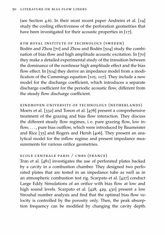
50 literature on bias flow liners
(see Section 4.6). In their most recent paper Andreini et al. [19]study the cooling effectiveness of the perforation geometries thathave been investigated for their acoustic properties in [17].
kth royal institute of technology (sweden)Bodén and Zhou [70] and Zhou and Bodén [504] study the combi-nation of bias flow and high amplitude acoustic excitation. In [70]they make a detailed experimental study of the transition betweenthe dominance of the nonlinear high amplitude effect and the biasflow effect. In [504] they derive an impedance model from a modi-fication of the Cummings equation [105, 107]. They include a newmodel for the discharge coefficient, which introduces a separatedischarge coefficient for the periodic acoustic flow, different fromthe steady flow discharge coefficient.
eindhoven university of technology (netherlands)Moers et al. [332] and Tonon et al. [478] present a comprehensivetreatment of the grazing and bias flow interaction. They discussthe different steady flow regimes, i. e. pure grazing flow, low in-flow, . . . , pure bias outflow, which were introduced by Baumeisterand Rice [35] and Rogers and Hersh [406]. They present an ana-lytical model for the inflow regime and present impedance mea-surements for various orifice geometries.
ecole centrale paris / cnrs (france)Tran et al. [481] investigates the use of perforated plates backedby a cavity in a combustion chamber. They designed two perfo-rated plates that are tested in an impedance tube as well as inan atmospheric combustion test rig. Scarpato et al. [427] conductLarge Eddy Simulations of an orifice with bias flow at low andhigh sound levels. Scarpato et al. [428, 429, 430] present a lowStrouhal number analysis and find that the optimal bias flow ve-locity is controlled by the porosity only. Then, the peak absorp-tion frequency can be modified by changing the cavity depth.
3.3 recent developments 51
They achieve a larger absorption bandwidth in the low Strouhalnumber regime and claim, that a low Strouhal number design isgenerally superior compared to previous efforts looking at theHelmholtz regime (e. g. [219]).
cambridge university (uk)Bhayaraju et al. [55] and Schmidt et al. [434] conduct acoustic mea-surements in a rectangular model combustor. The acoustic absorp-tion is measured for various perforation geometries and bias flowvelocities at ambient conditions with loudspeaker excitation. Incombustion tests, they evaluate the influence of the different per-foration geometries on the flame.
university of dayton (usa)Mazdeh and Kashani [317, 318] present results from an ongoingnumerical study. They are using Large Eddy Simulation (LES) andare working on including geometry parameters like the hole size,shape, orientation, and radius to thickness ratio. So far they havepresented impedance results while varying the thickness to radiusratio of the orifices. More results are announced to be presentedin future publications.
dlr german aerospace center (germany)Two optical measurement techniques, Particle Image Velocimetry(PIV) and Laser Doppler Anemometry (LDA), are applied to abias flow liner in [201]. This work is a joint effort with ONERAwho performed the LDA measurements. Both techniques deliversimilar results and are able to resolve the acoustic flow structuresin the vicinity of the orifice. A third optical technique is usedin a cooperation with TU Berlin and TU Dresden. Haufe et al.[191, 192] perform measurements applying Doppler Global Ve-locimetry with Frequency Modulation (FM-DGV). Schulz et al.[436] investigate the energy transfer with a spectral analysis ap-proach based on FM-DGV data. The results reveal a correlation
52 literature on bias flow liners
between the absorbed energy and the production of additionalspectral turbulence fluctuation components.
Heuwinkel et al. [200] and Lahiri et al. [280, 281] study the effectof an oscillating unsteady bias flow. The unsteady bias flow is gen-erated by a high amplitude acoustic excitation within the cavity ofthe liner. This new concept, the Zero Mass Flow Liner, promises adramatic reduction of the required mass flow rate while achievinga similar damping performance.
The comprehensive experimental parameter study with cylin-drical bias flow liners presented in [277, 279, 282] is the basis ofthis thesis. All details can be found in the following chapters.
3.4 chronological overview
Due to the large amount of publications addressing the bias floweffect, the previous sections only present a limited selection. Amore comprehensive overview is given in Table 3.1. The tableincludes not only the perforated liner setup, but various setupswhere the bias flow effect can be observed: single orifice, Helm-holtz resonator, perforated plate, sudden area expansion in a duct,duct termination, single-degree-of-freedom (SDOF) liner, double-degree-of-freedom (DDOF) liner. The nature of the work in thereferences can be mainly theoretical, experimental studies, andnumerical simulations, indicated by the cross in the T (theoret-ical), E (experimental), and S (simulation) columns, respectively.A ‘c’ in the experimental column indicates that combustion testshave been performed. For a quick reference, the last columns listsome common parameters that are addressed in each publication:frequency f, sound pressure level p′, bias flow Mach number Mb,grazing flow Mach number Mg, porosity σ, orifice diameter d,wall thickness t, orifice angle α, cavity volume V , and tempera-ture T .
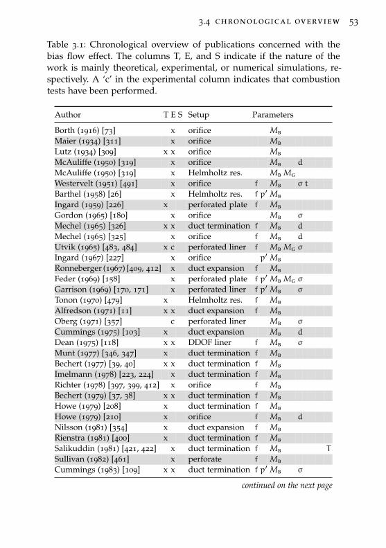
3.4 chronological overview 53
Table 3.1: Chronological overview of publications concerned with thebias flow effect. The columns T, E, and S indicate if the nature of thework is mainly theoretical, experimental, or numerical simulations, re-spectively. A ‘c’ in the experimental column indicates that combustiontests have been performed.
Author T E S Setup Parameters
Borth (1916) [73] x orifice MbMaier (1934) [311] x orifice MbLutz (1934) [309] x x orifice MbMcAuliffe (1950) [319] x orifice Mb d
McAuliffe (1950) [319] x Helmholtz res. Mb MgWestervelt (1951) [491] x orifice f Mb σ t
Barthel (1958) [26] x Helmholtz res. f p′ MbIngard (1959) [226] x perforated plate f MbGordon (1965) [180] x orifice Mb σ
Mechel (1965) [326] x x duct termination f Mb d
Mechel (1965) [325] x orifice f Mb d
Utvik (1965) [483, 484] x c perforated liner f Mb Mg σ
Ingard (1967) [227] x orifice p′ MbRonneberger (1967) [409, 412] x duct expansion f MbFeder (1969) [158] x perforated plate f p′ Mb Mg σ
Garrison (1969) [170, 171] x perforated liner f p′ Mb σ
Tonon (1970) [479] x Helmholtz res. f MbAlfredson (1971) [11] x x duct expansion f MbOberg (1971) [357] c perforated liner Mb σ
Cummings (1975) [103] x duct expansion Mb d
Dean (1975) [118] x x DDOF liner f Mb σ
Munt (1977) [346, 347] x duct termination f MbBechert (1977) [39, 40] x x duct termination f MbImelmann (1978) [223, 224] x duct termination f MbRichter (1978) [397, 399, 412] x orifice f MbBechert (1979) [37, 38] x x duct termination f MbHowe (1979) [208] x duct termination f MbHowe (1979) [210] x orifice f Mb d
Nilsson (1981) [354] x duct expansion f MbRienstra (1981) [400] x duct termination f MbSalikuddin (1981) [421, 422] x duct termination f Mb T
Sullivan (1982) [461] x perforate f MbCummings (1983) [109] x x duct termination f p′ Mb σ
continued on the next page
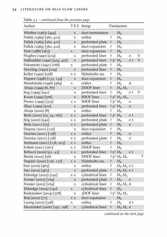
54 literature on bias flow liners
Table 3.1 – continued from the previous page
Author T E S Setup Parameters
Whiffen (1983) [494] x duct termination MbPallek (1984) [360, 412] x orifice f MbPallek (1984) [360, 412] x perforated plate f MbPallek (1984) [360, 412] x duct expansion f MbPeat (1988) [363] x duct expansion f MbHughes (1990) [219] x perforated liner f Mb σ V
Salikuddin (1990) [424, 425] x perforated liner f p′ Mb σ t V
Fukumoto (1991) [168] x perforated plate f MbDowling (1992) [129] x perforated liner f MbKeller (1995) [258] x x Helmholtz res. f MbDupere (1998) [133, 134] x duct expansion f MbWendoloski (1998) [489] x orifice f Mb d
Ahuja (1999) [6, 87] x DDOF liner f Mb MgJing (1999) [241] x perforated liner f Mb σ t V
Kwan (1999) [276] x SDOF liner f p′ Mb MgPremo (1999) [373] x x SDOF liner f p′ Mb σ
Zhao (1999) [502] x perforated liner f p′ Mb σ
Ahuja (2000) [8] x orifice f MbBetts (2000) [52, 54, 162] x x perforated liner f p′ Mb σ t
Jing (2000) [242] x x perforated plate f Mb σ t
Betts (2001) [53] x x perforated plate f Mb σ
Dupere (2001) [135] x duct expansion f MbDurrieu (2001) [138] x x orifice f Mb σ
Durrieu (2001) [138] x x perforated plate f Mb σ
Hofmans (2001) [138, 203] x x orifice f MbFollett (2001) [161] x x DDOF liner f MbBellucci (2002) [41, 43] x x perforated liner f p′ Mb σ t
Bielak (2002) [56] x DDOF liner f p′ Mb Mg T
Dupère (2002) [136, 137] x x Helmholtz res. f MbSun (2002) [463] x orifice f Mb Mg σ t
Sun (2002) [463] x perforated plate f Mb Mg σ t
Eldredge (2003) [142] x x cylindrical liner f Mb MgForster (2003) [164] x perforated plate f Mb σ
Forster (2003) [164] x cylindrical liner f Mb Mg d
Eldredge (2004) [140] x cylindrical liner f MbRademaker (2004) [378] x 3DOF liner f p′ Mb MgBoij (2005) [71] x x duct expansion MbLuong (2005) [308] x orifice f Mb d t
Heuwinkel (2006) [197, 198] x cylindrical liner f Mb Mg σ
continued on the next page
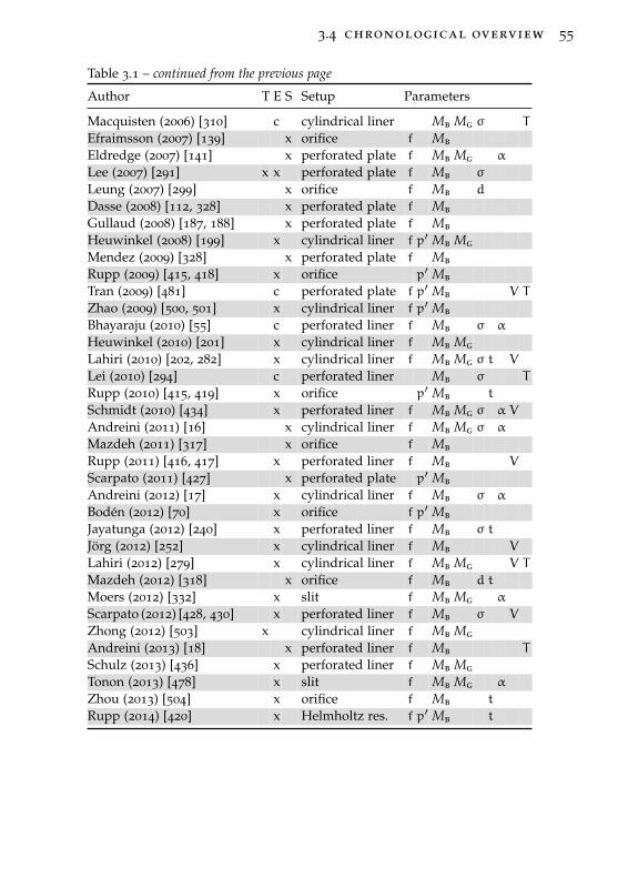
3.4 chronological overview 55
Table 3.1 – continued from the previous page
Author T E S Setup Parameters
Macquisten (2006) [310] c cylindrical liner Mb Mg σ T
Efraimsson (2007) [139] x orifice f MbEldredge (2007) [141] x perforated plate f Mb Mg α
Lee (2007) [291] x x perforated plate f Mb σ
Leung (2007) [299] x orifice f Mb d
Dasse (2008) [112, 328] x perforated plate f MbGullaud (2008) [187, 188] x perforated plate f MbHeuwinkel (2008) [199] x cylindrical liner f p′ Mb MgMendez (2009) [328] x perforated plate f MbRupp (2009) [415, 418] x orifice p′ MbTran (2009) [481] c perforated plate f p′ Mb V T
Zhao (2009) [500, 501] x cylindrical liner f p′ MbBhayaraju (2010) [55] c perforated liner f Mb σ α
Heuwinkel (2010) [201] x cylindrical liner f Mb MgLahiri (2010) [202, 282] x cylindrical liner f Mb Mg σ t V
Lei (2010) [294] c perforated liner Mb σ T
Rupp (2010) [415, 419] x orifice p′ Mb t
Schmidt (2010) [434] x perforated liner f Mb Mg σ α V
Andreini (2011) [16] x cylindrical liner f Mb Mg σ α
Mazdeh (2011) [317] x orifice f MbRupp (2011) [416, 417] x perforated liner f Mb V
Scarpato (2011) [427] x perforated plate p′ MbAndreini (2012) [17] x cylindrical liner f Mb σ α
Bodén (2012) [70] x orifice f p′ MbJayatunga (2012) [240] x perforated liner f Mb σ t
Jörg (2012) [252] x cylindrical liner f Mb V
Lahiri (2012) [279] x cylindrical liner f Mb Mg V T
Mazdeh (2012) [318] x orifice f Mb d t
Moers (2012) [332] x slit f Mb Mg α
Scarpato (2012) [428, 430] x perforated liner f Mb σ V
Zhong (2012) [503] x cylindrical liner f Mb MgAndreini (2013) [18] x perforated liner f Mb T
Schulz (2013) [436] x perforated liner f Mb MgTonon (2013) [478] x slit f Mb Mg α
Zhou (2013) [504] x orifice f Mb t
Rupp (2014) [420] x Helmholtz res. f p′ Mb t

4M O D E L I N G O F B I A S F L O W L I N E R S
4.1 rayleigh conductivity
The first attempt at a theoretical description of the acoustic prop-erties of an orifice was presented by Rayleigh [385, 390] when hewas studying Helmholtz resonators. He introduced the conceptof acoustic conductivity as an analogy to Ohm’s law1 in electricity.While the electric conductivity of a circuit element is describedby the ratio of the electric current to the potential difference, theacoustic conductivity of an orifice is given by the ratio of the vol-ume flow through the orifice to the driving pressure difference. Itis commonly referred to as Rayleigh conductivity2.
Let the fluctuating pressure on both sides of an orifice be aharmonic function of time, so that p′1 = Re{p1 e
iωt} for the fluc-tuating pressure above and p′2 = Re{p2 e
iωt} for the fluctuatingpressure below the orifice. Then, the pressure difference across theorifice Re{(p1 − p2) e
iωt} produces the fluctuating volume velocityq′ = Re{q eiωt} through the orifice. When the flow is regarded
1 Named after Georg Simon Ohm (1789-1854, German physicist and mathe-matician) [358].
2 Named after John William Strutt, Lord Rayleigh (1842-1919, English physi-cist).
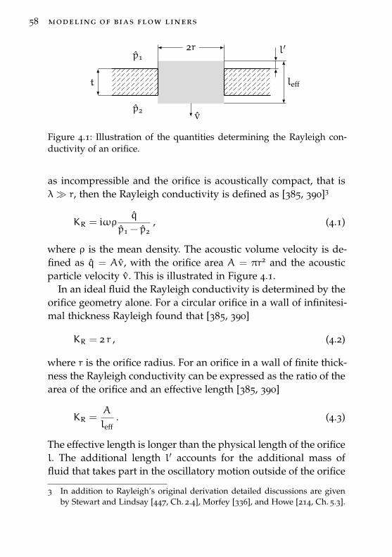
58 modeling of bias flow liners
draft – 2014.06.25 22:08 – claus lahiri
2r
t
l′
leff
v
p1
p2
Figure 4.1: Illustration of the quantities determining the Rayleigh con-ductivity of an orifice.
as incompressible and the orifice is acoustically compact, that isλ� r, then the Rayleigh conductivity is defined as [385, 390]3
KR = iωρq
p1 − p2, (4.1)
where ρ is the mean density. The acoustic volume velocity is de-fined as q = Av, with the orifice area A = πr2 and the acousticparticle velocity v. This is illustrated in Figure 4.1.
In an ideal fluid the Rayleigh conductivity is determined by theorifice geometry alone. For a circular orifice in a wall of infinitesi-mal thickness Rayleigh found that [385, 390]
KR = 2 r , (4.2)
where r is the orifice radius. For an orifice in a wall of finite thick-ness the Rayleigh conductivity can be expressed as the ratio of thearea of the orifice and an effective length [385, 390]
KR =A
leff. (4.3)
The effective length is longer than the physical length of the orificel. The additional length l′ accounts for the additional mass offluid that takes part in the oscillatory motion outside of the orifice
3 In addition to Rayleigh’s original derivation detailed discussions are givenby Stewart and Lindsay [447, Ch. 2.4], Morfey [336], and Howe [214, Ch. 5.3].
4.2 acoustic impedance 59
and is commonly referred to as end correction. This is illustratedin Figure 4.1. The effective length is defined as the sum of thephysical length of the orifice and the end correction for both ends:leff = l+ 2 l′.
In continuation, Rayleigh derives an upper and lower limit ofthe conductivity4 [385, 390]
π r2
l+ 163πr
< KR <πr2
l+ π2 r
(4.4)
For l = 0 the upper limit coincides with Equation (4.2) and theend correction can be determined from Equation (4.4) to be in therange 0.785 r < l′ < 0.849 r. In a further analysis Rayleigh [385,390] suggests l′ ≈ 0.82 r as the appropriate value for an orifice inan infinite wall. The exact value of the end correction has been anongoing topic of discussion. A generally accepted value for oneend of an orifice in a wall5 is [72, 100, 225, 260, 339]
l′ =8
3πr ≈ 0.85 r . (4.5)
While the end correction can be neglected for l� r it contributessubstantially when l→ 0.
4.2 acoustic impedance
The concept of acoustic impedance is similar6 to the Rayleigh con-ductivity, but allows a more comprehensive description of a dy-namic system. Originally, the impedance concept was introducedby Heaviside [193] for treating alternating currents of electricity.
4 A recent mathematical discussion of the limits is given by Laurens et al. [286].5 This configuration is often referred to as flanged pipe, in contrast to an un-
flanged pipe.6 It is shown in Appendix b.1, how the Rayleigh conductivity is converted into
an impedance.
60 modeling of bias flow liners
The electric impedance is defined by the ratio of voltage to currentand is measured in Ohm. It describes the opposition of an elementto transmit a current when a voltage is applied. Accordingly, theacoustic impedance is defined as the complex ratio of the acousticpressure to the acoustic volume velocity (Webster [487] or [369])
Z =p
q, (4.6)
Another form of impedance is given by the specific impedance
z =p
v. (4.7)
The specific impedance is related to the acoustic impedance byZ = z/A and is used to describe the acoustic properties of amedium or material, for example a perforated wall. Then, v is thenormal component of the acoustic particle velocity directed intothe surface. The specific impedance of a fluid is a characteristicquantity of the medium only and is therefore referred to as char-acteristic impedance z0. For plane waves z0 = ρc. A convenientdimensionless quantity is obtained by the ratio of specific andcharacteristic impedance, i. e. the normalized specific impedance
ζ = z/z0 . (4.8)
Mathematically, the impedance is represented by a complex num-ber7
Z = R+ iX , z = r+ ix , and ζ = θ+ iχ , (4.9)
where the real part is referred to as resistance and the imaginarypart as reactance.
7 The notation is for an eiωt time dependency. For a negative exponent theimaginary part in Equation (4.9) changes sign.
4.2 acoustic impedance 61
4.2.1 Impedance Modeling of Perforations
When the dimensions of an acoustic element, e. g. orifice, Helm-holtz resonator, etc., are much smaller than the relevant acousticwavelength, its characteristic behavior can be described by threeparameters: the resistance R, the inertance M, and the complianceC. The acoustic impedance can be written as the sum of thesethree quantities [260]
Z = R+ i [ωM− 1/(ωC)] . (4.10)
The three parameters R, M, and C are commonly referred to aslumped parameters and an element that complies with the acous-tic compact assumption is a lumped element.
In a mechanical system the resistance represents a linear, mass-less, viscous damper, the inertance corresponds to a lumped mass,and the compliance describes the reciprocal of the stiffness of alumped, linear, massless spring [156]. Generally, the resistance de-scribes the energy dissipation, while the reactive elements storeenergy, either in the form of potential energy in a spring-like ele-ment or kinetic energy in a mass-like element [338].
Now, the process of building up an impedance model of a per-forate is demonstrated. Similar, but more detailed derivation canbe found in [271, 327].
Internal Impedance
First, the impedance within an orifice is considered, without anyend effects. The normalized specific impedance for a unit length lof an infinite tube filled with a viscous fluid is given by (Crandall[100] or [327])
ζ =1σ
iklF(k′sr)
. (4.11)
62 modeling of bias flow liners
The division by the porosity σ converts the impedance of a singleorifice into the impedance of an array of orifices in a perforation8.ikl is the inviscid impedance of an infinite tube. It describes theinertia of the oscillating mass of air. The function F introducesthe viscous effects. Based on the theories given by Stokes [451],Helmholtz [195], and Kirchhoff [261], which are presented in Sec-tion 5.4.1, Crandall [100, Appx. A] derives
F(x) = 1 −2 J1(x)x J0(x)
, (4.12)
where J0 and J1 are Bessel functions9 of the first kind. The effectiveStokes wave number10 k′s considers the viscosity as well as ther-mal conductivity losses near a highly conducting wall. In order toinclude both effects an effective kinematic viscosity ν′ = 2.179νis used, so that k′s =
√−iω/ν′. Sometimes the heat conduction is
neglected entirely, then ν′ is replaced by ν.The Bessel functions with a complex argument produces a com-plex result, so that the impedance consists of a reactive and re-sistive part. Unfortunately, more physical insight is not providedby Equation (4.11). However, two approximations do exist, whichare more physically revealing. Depending on the shear numberSh = r
√ω/ν they yield [100, 327]:
ζ ≈ 8νlcσr2 + i
k
σ
(l+
13l
)for Sh < 2 (4.13)
ζ ≈√
2ωνlcσr
+ i(kl
σ+
√2ωνlcσr
)for Sh > 10 (4.14)
8 Often, the impedance is divided also by the discharge coefficient, e. g. [271].However, this was not done traditionally, e. g. [100, 327].
9 Named after Friedrich Wilhelm Bessel (1784-1846, German mathematicianand astronomer). Bessel functions are the solutions to the Bessel differentialequation [51]. They are a standard mathematical tool when dealing withcylindrical geometries, e.g. [3, 77].
10 Named after Sir George Gabriel Stokes (1819-1903, Irish mathematician andphysicist.
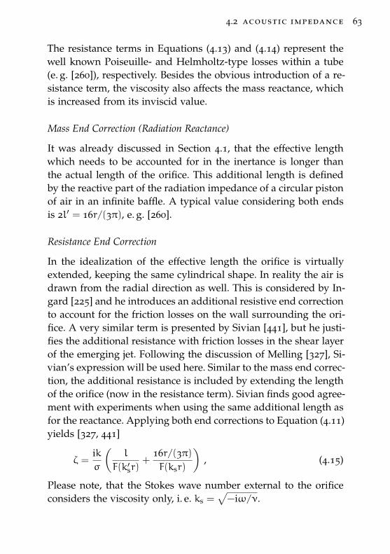
4.2 acoustic impedance 63
The resistance terms in Equations (4.13) and (4.14) represent thewell known Poiseuille- and Helmholtz-type losses within a tube(e. g. [260]), respectively. Besides the obvious introduction of a re-sistance term, the viscosity also affects the mass reactance, whichis increased from its inviscid value.
Mass End Correction (Radiation Reactance)
It was already discussed in Section 4.1, that the effective lengthwhich needs to be accounted for in the inertance is longer thanthe actual length of the orifice. This additional length is definedby the reactive part of the radiation impedance of a circular pistonof air in an infinite baffle. A typical value considering both endsis 2l′ = 16r/(3π), e. g. [260].
Resistance End Correction
In the idealization of the effective length the orifice is virtuallyextended, keeping the same cylindrical shape. In reality the air isdrawn from the radial direction as well. This is considered by In-gard [225] and he introduces an additional resistive end correctionto account for the friction losses on the wall surrounding the ori-fice. A very similar term is presented by Sivian [441], but he justi-fies the additional resistance with friction losses in the shear layerof the emerging jet. Following the discussion of Melling [327], Si-vian’s expression will be used here. Similar to the mass end correc-tion, the additional resistance is included by extending the lengthof the orifice (now in the resistance term). Sivian finds good agree-ment with experiments when using the same additional length asfor the reactance. Applying both end corrections to Equation (4.11)yields [327, 441]
ζ =ikσ
(l
F(k′sr)+
16r/(3π)F(ksr)
), (4.15)
Please note, that the Stokes wave number external to the orificeconsiders the viscosity only, i. e. ks =
√−iω/ν.
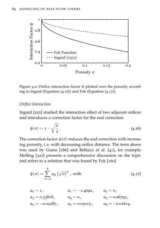
64 modeling of bias flow liners
0 0.05 0.1 0.15 0.20.2
0.4
0.6
0.8
1
Porosity σ
Inte
ract
ion
Fact
orψ
Fok FunctionIngard (1953)
Figure 4.2: Orifice interaction factor ψ plotted over the porosity accord-ing to Ingard (Equation (4.16)) and Fok (Equation (4.17)).
Orifice Interaction
Ingard [225] studied the interaction effect of two adjacent orificesand introduces a correction factor for the end correction
ψ(σ) = 1 −
√σ
2. (4.16)
The correction factor ψ(σ) reduces the end correction with increas-ing porosity, i. e. with decreasing orifice distance. The term abovewas used by Guess [186] and Bellucci et al. [41], for example.Melling [327] presents a comprehensive discussion on the topicand refers to a solution that was found by Fok [160]
ψ(σ) =
8∑n=0
an(√σ)n , with (4.17)
a0 = 1 , a1 = −1.4092 , a2 = 0 ,
a3 = 0.33818 , a4 = 0 , a5 = 0.06793 ,
a6 = −0.02287 , a7 = 0.03015 , a8 = −0.01614 .
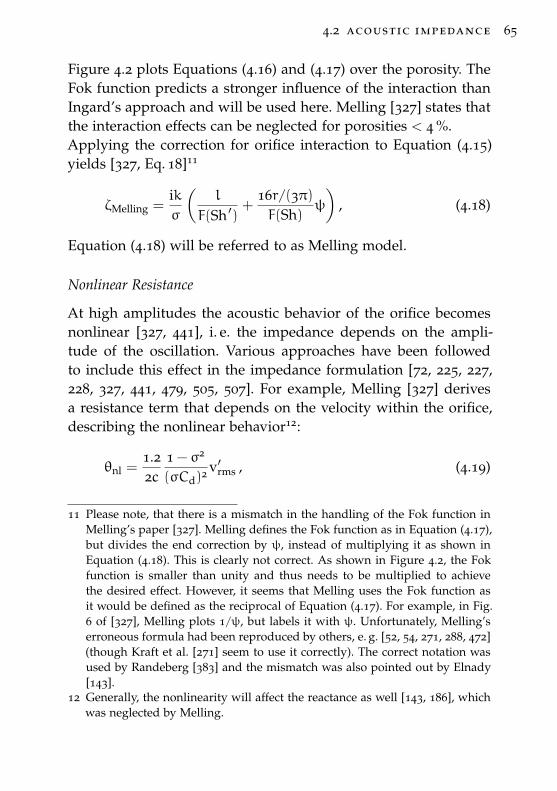
4.2 acoustic impedance 65
Figure 4.2 plots Equations (4.16) and (4.17) over the porosity. TheFok function predicts a stronger influence of the interaction thanIngard’s approach and will be used here. Melling [327] states thatthe interaction effects can be neglected for porosities < 4 %.Applying the correction for orifice interaction to Equation (4.15)yields [327, Eq. 18]11
ζMelling =ikσ
(l
F(Sh ′)+
16r/(3π)F(Sh)
ψ
), (4.18)
Equation (4.18) will be referred to as Melling model.
Nonlinear Resistance
At high amplitudes the acoustic behavior of the orifice becomesnonlinear [327, 441], i. e. the impedance depends on the ampli-tude of the oscillation. Various approaches have been followedto include this effect in the impedance formulation [72, 225, 227,228, 327, 441, 479, 505, 507]. For example, Melling [327] derivesa resistance term that depends on the velocity within the orifice,describing the nonlinear behavior12:
θnl =1.22c
1 − σ2
(σCd)2 v′rms , (4.19)
11 Please note, that there is a mismatch in the handling of the Fok function inMelling’s paper [327]. Melling defines the Fok function as in Equation (4.17),but divides the end correction by ψ, instead of multiplying it as shown inEquation (4.18). This is clearly not correct. As shown in Figure 4.2, the Fokfunction is smaller than unity and thus needs to be multiplied to achievethe desired effect. However, it seems that Melling uses the Fok function asit would be defined as the reciprocal of Equation (4.17). For example, in Fig.6 of [327], Melling plots 1/ψ, but labels it with ψ. Unfortunately, Melling’serroneous formula had been reproduced by others, e. g. [52, 54, 271, 288, 472](though Kraft et al. [271] seem to use it correctly). The correct notation wasused by Randeberg [383] and the mismatch was also pointed out by Elnady[143].
12 Generally, the nonlinearity will affect the reactance as well [143, 186], whichwas neglected by Melling.
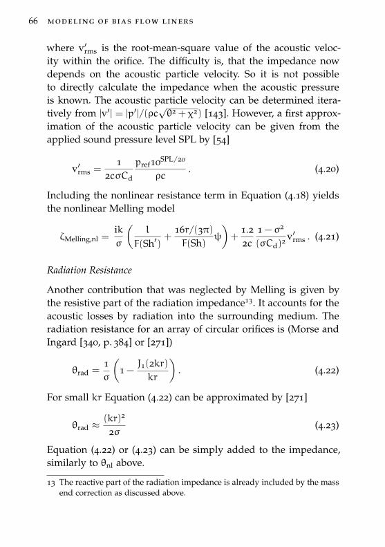
66 modeling of bias flow liners
where v′rms is the root-mean-square value of the acoustic veloc-ity within the orifice. The difficulty is, that the impedance nowdepends on the acoustic particle velocity. So it is not possibleto directly calculate the impedance when the acoustic pressureis known. The acoustic particle velocity can be determined itera-tively from |v′| = |p′|/(ρc
√θ2 + χ2) [143]. However, a first approx-
imation of the acoustic particle velocity can be given from theapplied sound pressure level SPL by [54]
v′rms =1
2cσCd
pref10SPL/20
ρc. (4.20)
Including the nonlinear resistance term in Equation (4.18) yieldsthe nonlinear Melling model
ζMelling,nl =ikσ
(l
F(Sh′)+
16r/(3π)F(Sh)
ψ
)+
1.22c
1 − σ2
(σCd)2 v′rms . (4.21)
Radiation Resistance
Another contribution that was neglected by Melling is given bythe resistive part of the radiation impedance13. It accounts for theacoustic losses by radiation into the surrounding medium. Theradiation resistance for an array of circular orifices is (Morse andIngard [340, p. 384] or [271])
θrad =1σ
(1 −
J1(2kr)kr
). (4.22)
For small kr Equation (4.22) can be approximated by [271]
θrad ≈(kr)2
2σ(4.23)
Equation (4.22) or (4.23) can be simply added to the impedance,similarly to θnl above.
13 The reactive part of the radiation impedance is already included by the massend correction as discussed above.
4.2 acoustic impedance 67
4.2.2 Grazing Flow Impedance
The effect of grazing flow on the impedance is often accounted forby a simple contribution to the resistance [34, 186, 194, 392]14
θg =0.3 Mg
σ(4.24)
More sophisticated models are available, e. g. [106, 181, 209, 244,266, 290]. Especially the importance of the friction velocity, ratherthan the mean flow velocity, has been studied [175, 194]. However,Peat et al. [364] conclude that the influence of the friction velocityis of no significance when the boundary layer is turbulent andfully developed. That is the case for the measurements presentedhere, so that the use of the mean velocity is adequate and thesimple model of Equation (4.24) is sufficient. It should be noted,that Equation (4.24) neglects the reduction of the attached massby the grazing flow.
4.2.3 Bias Flow Impedance
Traditionally, there are two alternatives to include the influence ofa steady bias flow on the impedance of an orifice or perforation.In the first approach the acoustic particle velocity in a nonlinearmodel is replaced by the bias flow velocity [34, 118, 171, 227, 326,459, 505]. This replacement is only reasonable if the bias flow ve-locity is assumed to be much greater than the acoustic particlevelocity. For a simple linear relationship of resistance and biasflow Mach number given by Sivian [441] this yields
θb =C ·Mb
σ(4.25)
and is very similar to the grazing flow resistance introduced inEquation (4.24). C is a constant that is based on empiricism and
14 The factor of 0.3 is most common. However, some variations can be found inthe literature, for example Rice [392] suggests 0.5.
68 modeling of bias flow liners
is in the range 1 − 1.5, typically 1.15 [34]15. For a steady bias flowCummings and Eversman [109] derive C = (1 − σ2C2
c)/C2c from
the linearized Bernoulli equation, where Cc is the contraction co-efficient of the jet.
The second approach combines the effects of the acoustic par-ticle velocity and the steady bias flow velocity in one resistanceterm. For example, Premo [373] suggests a combined velocity termof√
(1.15 v′rms)2 + (2Ub)2. Betts [52, 54] finds the similar expres-
sion |1.2 v′rms + 2Ub|. Adding this to Equation (4.19) yields
θb =12c
1 − σ2
(σCd)2 |1.2 v′rms + 2Ub| (4.26)
Both approaches are mostly based on empiricism and lack theinfluence of the bias flow on the reactance.
More advanced approaches are presented by Jing and Sun [242]and Lee et al. [291]. However, both need to be solved numerically,so that they do not provide a simple parametric description of theimpedance. Jing and Sun [242] solve Howe’s [210] governing equa-tions with a boundary element method. Howe himself obtains ananalytical solution when assuming infinitesimal thickness and acylindrical vortex sheet (see Section 4.3 below). Jing and Sun [242]include a finite thickness and allow a contraction of the vortexsheet, which requires a numerical solution of the equations. Leeet al. [291] determine the impedance of a perforated plate by solv-ing the incompressible Euler equation. In particular, they considerthe interaction effect.
4.3 howe rayleigh conductivity model
Howe [210, 214] analytically derives a formulation of the Rayleighconductivity for an orifice with a bias flow and includes the ab-
15 This value is often accredited to Bauer [34]. However, Bauer himself refer-ences Zinn [505]. Both, Zinn [505] and Bauer [34], use this term to describehigh amplitude effects, not a steady bias flow. See as well the discussion inSection 4.6.
4.3 howe rayleigh conductivity model 69
sorption caused by vorticity shedding. He treats a single, circularorifice in a wall of infinitesimal thickness. On the inlet side theflow field resembles that of a potential sink at the center of theorifice and on the outlet side that of an axisymmetric jet flow witha potential core and shear layer. Viscosity is neglected except atthe rims of the orifice, where the acoustic perturbations triggerthe periodical shedding of vortex rings. The convection velocityof the vortex rings is taken to be the mean velocity within theorifice. The radius of the vortex rings coincides with the orifice ra-dius and remains constant when traveling downstream, forminga cylindrical vortex sheet. The assumptions can be summarized:
1. The frequency of the sound is low, so that the wavelength ismuch larger than the orifice radius (the orifice is acousticallycompact)16: λ� r
2. The Mach number of the bias flow is low, so that the fluidcan be considered incompressible17: Mb � 1
3. The Reynolds number of the bias flow is high, so that viscos-ity is only considered at the rims of the orifice18: Ub r/ν� 1
4. The wall is infinitely thin: t = 0
After a lengthy derivation Howe arrives at [210, 214]19
KR = 2r(γ+ iδ) (4.27)
16 For the largest orifice dimension treated in the parameter study here (r =
1.25 mm), this yields a frequency limit of f � 272360 Hz at standard tem-perature and pressure conditions. Higher temperatures and smaller radii in-creases the limit further.
17 Typically, Mb < 0.3.18 The highest limit is given at high temperature, low pressure, and small
radius. The extreme values of the parameter study here (T = 823.15 K,p = 101.325 kPa, r = 0.5 mm) restrict the applicability of Howe’s model toMb � 0.0003.
19 Here, the sign is adjusted to the eiωt convention.
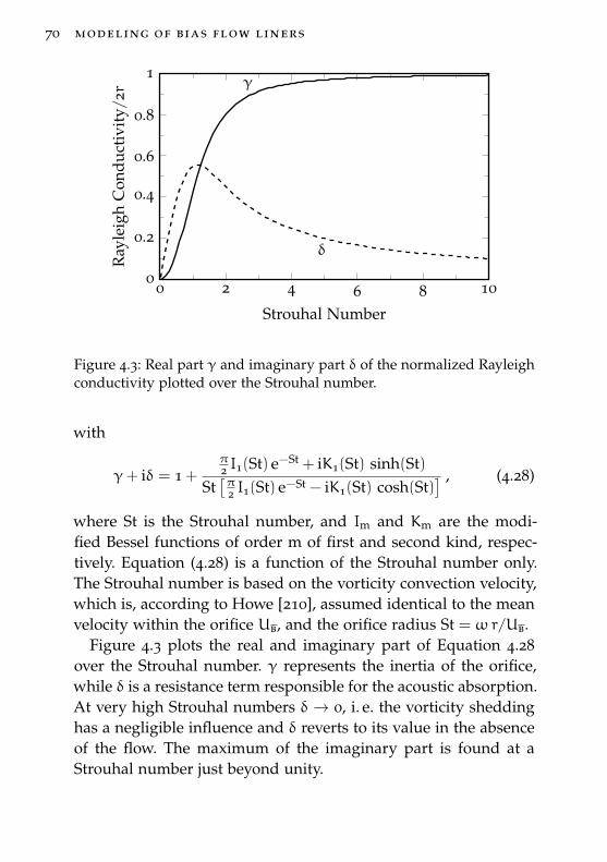
70 modeling of bias flow liners
0 2 4 6 8 100
0.2
0.4
0.6
0.8
1γ
δ
Strouhal Number
Ray
leig
hC
ondu
ctiv
ity/
2r
Figure 4.3: Real part γ and imaginary part δ of the normalized Rayleighconductivity plotted over the Strouhal number.
with
γ+ iδ = 1 +π2 I1(St) e−St + iK1(St) sinh(St)
St[π2 I1(St) e−St − iK1(St) cosh(St)
] , (4.28)
where St is the Strouhal number, and Im and Km are the modi-fied Bessel functions of order m of first and second kind, respec-tively. Equation (4.28) is a function of the Strouhal number only.The Strouhal number is based on the vorticity convection velocity,which is, according to Howe [210], assumed identical to the meanvelocity within the orifice Ub, and the orifice radius St = ωr/Ub.
Figure 4.3 plots the real and imaginary part of Equation 4.28over the Strouhal number. γ represents the inertia of the orifice,while δ is a resistance term responsible for the acoustic absorption.At very high Strouhal numbers δ → 0, i. e. the vorticity sheddinghas a negligible influence and δ reverts to its value in the absenceof the flow. The maximum of the imaginary part is found at aStrouhal number just beyond unity.
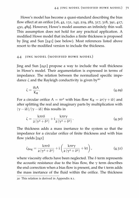
4.4 jing model (modified howe model) 71
Howe’s model has become a quasi-standard describing the biasflow effect at an orifice [16, 42, 131, 142, 219, 282, 317, 318, 391, 417,430, 489]. However, Howe’s model assumes an infinitely thin wall.This assumption does not hold for any practical application. Amodified Howe model that includes a finite thickness is proposedby Jing and Sun [241] (see below). Most references listed aboveresort to the modified version to include the thickness.
4.4 jing model (modified howe model)
Jing and Sun [241] propose a way to include the wall thicknessin Howe’s model. Their argumentation is expressed in terms ofimpedance. The relation between the normalized specific impe-dance ζ and the Rayleigh conductivity is given by20
ζ =ikAKR
. (4.29)
For a circular orifice A = πr2 with bias flow KR = 2r(γ+ iδ) andafter splitting the real and imaginary parts by multiplication with(γ− iδ)/(γ− iδ) this results in
ζ =kπrδ
2 (γ2 + δ2)+ i
kπrγ
2 (γ2 + δ2). (4.30)
The thickness adds a mass inertance to the system so that theimpedance for a circular orifice of finite thickness and with biasflow yields [241]
ζJing =kπrδ
2 (γ2 + δ2)+ i(
kπrγ
2 (γ2 + δ2)+ kt
), (4.31)
where viscosity effects have been neglected. The δ term representsthe acoustic resistance due to the bias flow, the γ term describesthe end correction when a bias flow is present, and the t term addsthe mass inertance of the fluid within the orifice. The thickness
20 This relation is derived in Appendix b.1.
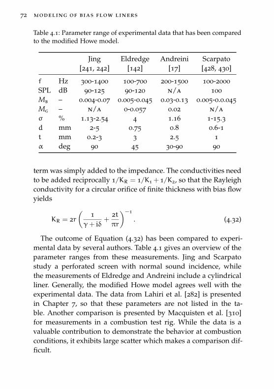
72 modeling of bias flow liners
Table 4.1: Parameter range of experimental data that has been comparedto the modified Howe model.
Jing Eldredge Andreini Scarpato[241, 242] [142] [17] [428, 430]
f Hz 300-1400 100-700 200-1500 100-2000SPL dB 90-125 90-120 n/a 100Mb – 0.004-0.07 0.005-0.045 0.03-0.13 0.005-0.0.045Mg – n/a 0-0.057 0.02 n/aσ % 1.13-2.54 4 1.16 1-15.3d mm 2-5 0.75 0.8 0.6-1t mm 0.2-3 3 2.5 1α deg 90 45 30-90 90
term was simply added to the impedance. The conductivities needto be added reciprocally 1/KR = 1/K1 + 1/K2, so that the Rayleighconductivity for a circular orifice of finite thickness with bias flowyields
KR = 2r(
1γ+ iδ
+2tπr
)−1
. (4.32)
The outcome of Equation (4.32) has been compared to experi-mental data by several authors. Table 4.1 gives an overview of theparameter ranges from these measurements. Jing and Scarpatostudy a perforated screen with normal sound incidence, whilethe measurements of Eldredge and Andreini include a cylindricalliner. Generally, the modified Howe model agrees well with theexperimental data. The data from Lahiri et al. [282] is presentedin Chapter 7, so that these parameters are not listed in the ta-ble. Another comparison is presented by Macquisten et al. [310]for measurements in a combustion test rig. While the data is avaluable contribution to demonstrate the behavior at combustionconditions, it exhibits large scatter which makes a comparison dif-ficult.
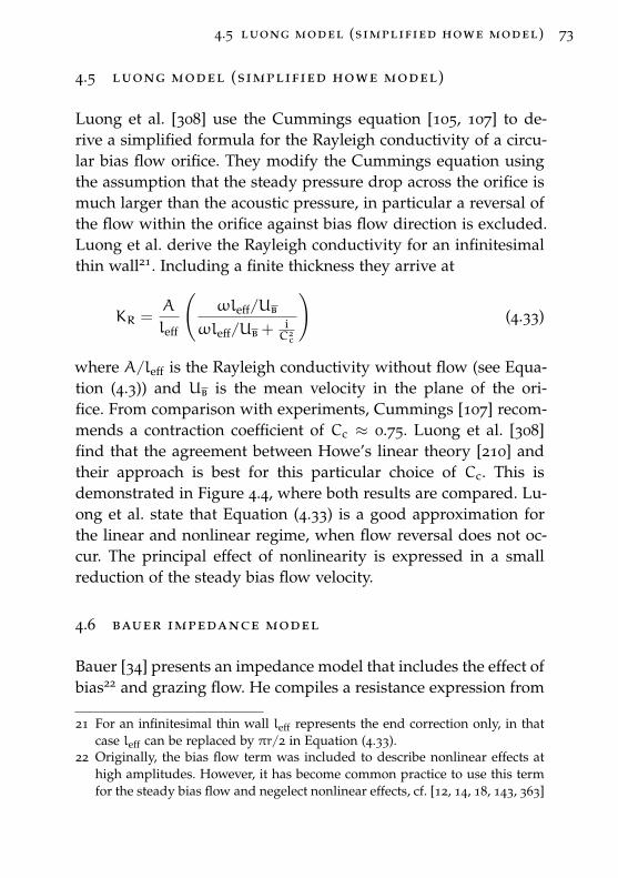
4.5 luong model (simplified howe model) 73
4.5 luong model (simplified howe model)
Luong et al. [308] use the Cummings equation [105, 107] to de-rive a simplified formula for the Rayleigh conductivity of a circu-lar bias flow orifice. They modify the Cummings equation usingthe assumption that the steady pressure drop across the orifice ismuch larger than the acoustic pressure, in particular a reversal ofthe flow within the orifice against bias flow direction is excluded.Luong et al. derive the Rayleigh conductivity for an infinitesimalthin wall21. Including a finite thickness they arrive at
KR =A
leff
(ωleff/Ub
ωleff/Ub +iC2c
)(4.33)
where A/leff is the Rayleigh conductivity without flow (see Equa-tion (4.3)) and Ub is the mean velocity in the plane of the ori-fice. From comparison with experiments, Cummings [107] recom-mends a contraction coefficient of Cc ≈ 0.75. Luong et al. [308]find that the agreement between Howe’s linear theory [210] andtheir approach is best for this particular choice of Cc. This isdemonstrated in Figure 4.4, where both results are compared. Lu-ong et al. state that Equation (4.33) is a good approximation forthe linear and nonlinear regime, when flow reversal does not oc-cur. The principal effect of nonlinearity is expressed in a smallreduction of the steady bias flow velocity.
4.6 bauer impedance model
Bauer [34] presents an impedance model that includes the effect ofbias22 and grazing flow. He compiles a resistance expression from
21 For an infinitesimal thin wall leff represents the end correction only, in thatcase leff can be replaced by πr/2 in Equation (4.33).
22 Originally, the bias flow term was included to describe nonlinear effects athigh amplitudes. However, it has become common practice to use this termfor the steady bias flow and negelect nonlinear effects, cf. [12, 14, 18, 143, 363]
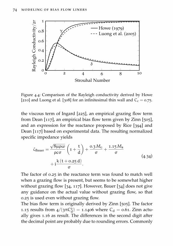
74 modeling of bias flow liners
0 2 4 6 8 100
0.2
0.4
0.6
0.8
1
γ
δ
Strouhal Number
Ray
leig
hC
ondu
ctiv
ity/
2rHowe (1979)Luong et al. (2005)
Figure 4.4: Comparison of the Rayleigh conductivity derived by Howe[210] and Luong et al. [308] for an infinitesimal thin wall and Cc = 0.75.
the viscous term of Ingard [225], an empirical grazing flow termfrom Dean [117], an empirical bias flow term given by Zinn [505],and an expression for the reactance proposed by Rice [394] andDean [117] based on experimental data. The resulting normalizedspecific impedance yields
ζBauer =
√8µρωρcσ
(1 +
t
d
)+
0.3 Mg
σ+
1.15 Mb
σ
+ ik (t+ 0.25d)
σ.
(4.34)
The factor of 0.25 in the reactance term was found to match wellwhen a grazing flow is present, but seems to be somewhat higherwithout grazing flow [34, 117]. However, Bauer [34] does not giveany guidance on the actual value without grazing flow, so that0.25 is used even without grazing flow.The bias flow term is originally derived by Zinn [505]. The factor1.15 results from 4/(3πC2
d) = 1.1406 where Cd = 0.61. Zinn actu-ally gives 1.16 as result. The differences in the second digit afterthe decimal point are probably due to rounding errors. Commonly
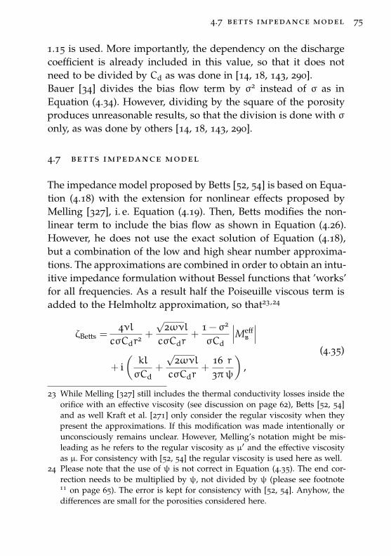
4.7 betts impedance model 75
1.15 is used. More importantly, the dependency on the dischargecoefficient is already included in this value, so that it does notneed to be divided by Cd as was done in [14, 18, 143, 290].Bauer [34] divides the bias flow term by σ2 instead of σ as inEquation (4.34). However, dividing by the square of the porosityproduces unreasonable results, so that the division is done with σonly, as was done by others [14, 18, 143, 290].
4.7 betts impedance model
The impedance model proposed by Betts [52, 54] is based on Equa-tion (4.18) with the extension for nonlinear effects proposed byMelling [327], i. e. Equation (4.19). Then, Betts modifies the non-linear term to include the bias flow as shown in Equation (4.26).However, he does not use the exact solution of Equation (4.18),but a combination of the low and high shear number approxima-tions. The approximations are combined in order to obtain an intu-itive impedance formulation without Bessel functions that ’works’for all frequencies. As a result half the Poiseuille viscous term isadded to the Helmholtz approximation, so that23,24
ζBetts =4νl
cσCdr2 +
√2ωνlcσCdr
+1 − σ2
σCd
∣∣∣Meffb
∣∣∣+ i(kl
σCd+
√2ωνlcσCdr
+163πr
ψ
),
(4.35)
23 While Melling [327] still includes the thermal conductivity losses inside theorifice with an effective viscosity (see discussion on page 62), Betts [52, 54]and as well Kraft et al. [271] only consider the regular viscosity when theypresent the approximations. If this modification was made intentionally orunconsciously remains unclear. However, Melling’s notation might be mis-leading as he refers to the regular viscosity as µ′ and the effective viscosityas µ. For consistency with [52, 54] the regular viscosity is used here as well.
24 Please note that the use of ψ is not correct in Equation (4.35). The end cor-rection needs to be multiplied by ψ, not divided by ψ (please see footnote11 on page 65). The error is kept for consistency with [52, 54]. Anyhow, thedifferences are small for the porosities considered here.
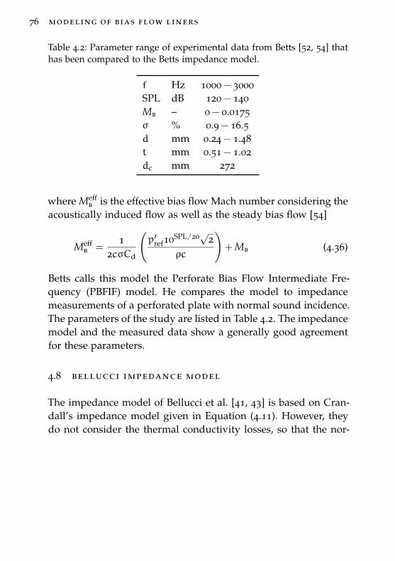
76 modeling of bias flow liners
Table 4.2: Parameter range of experimental data from Betts [52, 54] thathas been compared to the Betts impedance model.
f Hz 1000 − 3000SPL dB 120 − 140Mb – 0 − 0.0175σ % 0.9 − 16.5d mm 0.24 − 1.48t mm 0.51 − 1.02dc mm 272
where Meffb is the effective bias flow Mach number considering the
acoustically induced flow as well as the steady bias flow [54]
Meffb =
12cσCd
(p′ref10SPL/20√2
ρc
)+ Mb (4.36)
Betts calls this model the Perforate Bias Flow Intermediate Fre-quency (PBFIF) model. He compares the model to impedancemeasurements of a perforated plate with normal sound incidence.The parameters of the study are listed in Table 4.2. The impedancemodel and the measured data show a generally good agreementfor these parameters.
4.8 bellucci impedance model
The impedance model of Bellucci et al. [41, 43] is based on Cran-dall’s impedance model given in Equation (4.11). However, theydo not consider the thermal conductivity losses, so that the nor-
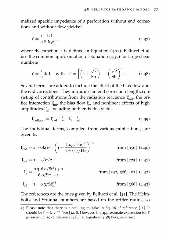
4.8 bellucci impedance model 77
malized specific impedance of a perforation without end correc-tions and without flow yields25
ζ =1σ
iklF(ksr)
, (4.37)
where the function F is defined in Equation (4.12). Bellucci et al.use the common approximation of Equation (4.37) for large shearnumbers
ζ =1σ
iklΓ with Γ =
[(1 +
√2
Sh
)− i(√
2Sh
)]. (4.38)
Several terms are added to include the effect of the bias flow andthe end corrections. They introduce an end correction length, con-sisting of contributions from the radiation reactance l′rad, the ori-fice interaction l′int, the bias flow l′b, and nonlinear effects of highamplitudes l′nl. Including both ends this yields
l′Bellucci = l′rad · l′int · l′b · l′nl . (4.39)
The individual terms, compiled from various publications, aregiven by:
l′rad = 2 · 0.8216 r(
1 +(0.77 He)2
1 + 0.77 He
)−1
from [356] (4.40)
l′int = 1 −√σ/2 from [225] (4.41)
l′b =0.3(6.0/St2) + 1
6.0/St2 + 1from [242, 366, 401] (4.42)
l′nl = 1 − 0.3/St0.6ac from [366] (4.43)
The references are the ones given by Bellucci et al. [41]. The Helm-holtz and Strouhal numbers are based on the orifice radius, so
25 Please note that there is a spelling mistake in Eq. 18 of reference [41]. Itshould be Γ = [. . . ]−1 (see [327]). However, the approximate expression for Γgiven in Eq. 19 of reference [41], i. e. Equation (4.38) here, is correct.
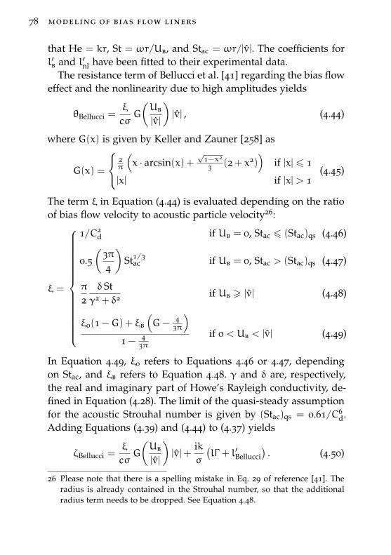
78 modeling of bias flow liners
that He = kr, St = ωr/Ub, and Stac = ωr/|v|. The coefficients forl′b and l′nl have been fitted to their experimental data.
The resistance term of Bellucci et al. [41] regarding the bias floweffect and the nonlinearity due to high amplitudes yields
θBellucci =ξ
cσG
(Ub
|v|
)|v| , (4.44)
where G(x) is given by Keller and Zauner [258] as
G(x) =
2π
(x · arcsin(x) +
√1−x2
3 (2 + x2))
if |x| 6 1
|x| if |x| > 1(4.45)
The term ξ in Equation (4.44) is evaluated depending on the ratioof bias flow velocity to acoustic particle velocity26:
ξ =
1/C2d if Ub = 0, Stac 6 (Stac)qs (4.46)
0.5(
3π4
)St1/3
ac if Ub = 0, Stac > (Stac)qs (4.47)
π
2δ St
γ2 + δ2 if Ub > |v| (4.48)
ξ0(1 −G) + ξb
(G− 4
3π
)1 − 4
3πif 0 < Ub < |v| (4.49)
In Equation 4.49, ξ0 refers to Equations 4.46 or 4.47, dependingon Stac, and ξb refers to Equation 4.48. γ and δ are, respectively,the real and imaginary part of Howe’s Rayleigh conductivity, de-fined in Equation (4.28). The limit of the quasi-steady assumptionfor the acoustic Strouhal number is given by (Stac)qs = 0.61/C6
d.Adding Equations (4.39) and (4.44) to (4.37) yields
ζBellucci =ξ
cσG
(Ub
|v|
)|v|+
ikσ
(lΓ + l′Bellucci
). (4.50)
26 Please note that there is a spelling mistake in Eq. 29 of reference [41]. Theradius is already contained in the Strouhal number, so that the additionalradius term needs to be dropped. See Equation 4.48.
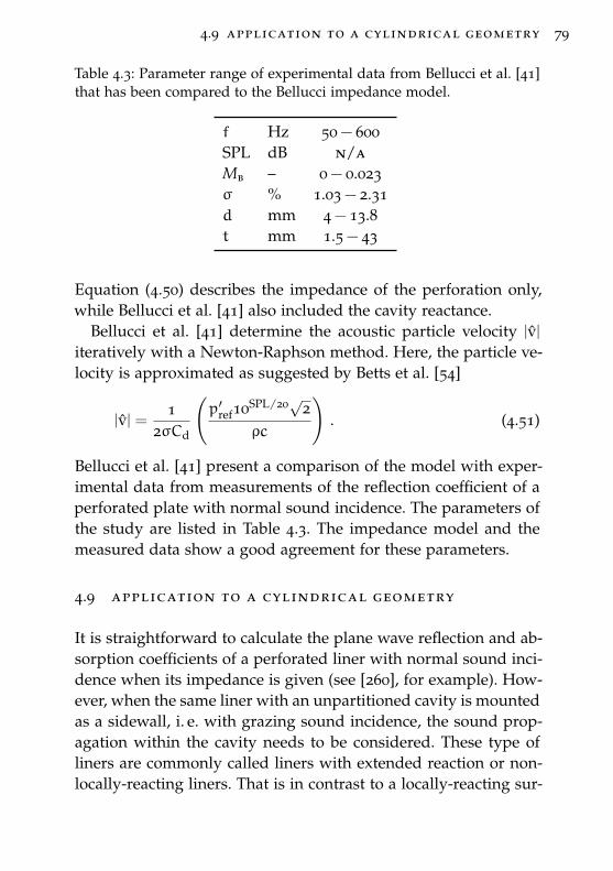
4.9 application to a cylindrical geometry 79
Table 4.3: Parameter range of experimental data from Bellucci et al. [41]that has been compared to the Bellucci impedance model.
f Hz 50 − 600SPL dB n/aMb – 0 − 0.023σ % 1.03 − 2.31d mm 4 − 13.8t mm 1.5 − 43
Equation (4.50) describes the impedance of the perforation only,while Bellucci et al. [41] also included the cavity reactance.
Bellucci et al. [41] determine the acoustic particle velocity |v|iteratively with a Newton-Raphson method. Here, the particle ve-locity is approximated as suggested by Betts et al. [54]
|v| =1
2σCd
(p′ref10SPL/20√2
ρc
). (4.51)
Bellucci et al. [41] present a comparison of the model with exper-imental data from measurements of the reflection coefficient of aperforated plate with normal sound incidence. The parameters ofthe study are listed in Table 4.3. The impedance model and themeasured data show a good agreement for these parameters.
4.9 application to a cylindrical geometry
It is straightforward to calculate the plane wave reflection and ab-sorption coefficients of a perforated liner with normal sound inci-dence when its impedance is given (see [260], for example). How-ever, when the same liner with an unpartitioned cavity is mountedas a sidewall, i. e. with grazing sound incidence, the sound prop-agation within the cavity needs to be considered. These type ofliners are commonly called liners with extended reaction or non-locally-reacting liners. That is in contrast to a locally-reacting sur-
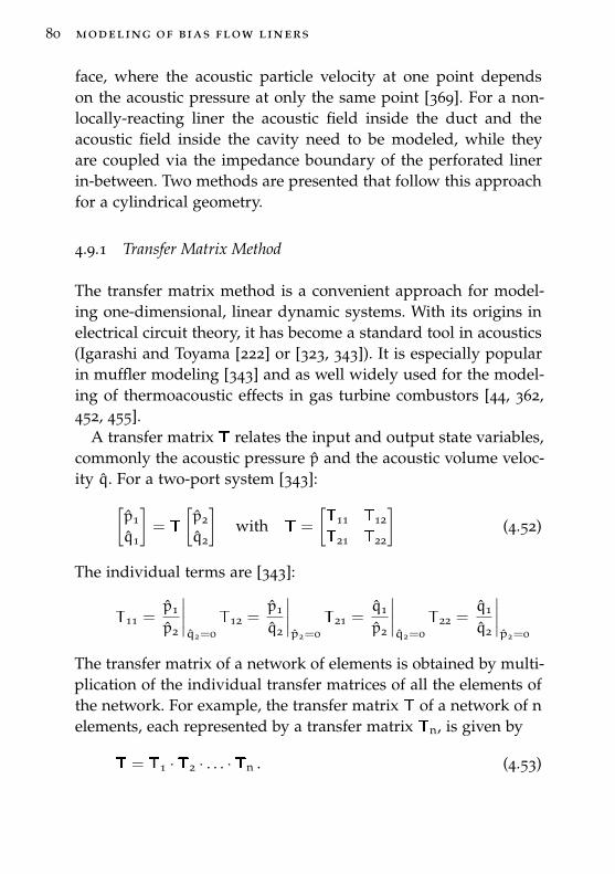
80 modeling of bias flow liners
face, where the acoustic particle velocity at one point dependson the acoustic pressure at only the same point [369]. For a non-locally-reacting liner the acoustic field inside the duct and theacoustic field inside the cavity need to be modeled, while theyare coupled via the impedance boundary of the perforated linerin-between. Two methods are presented that follow this approachfor a cylindrical geometry.
4.9.1 Transfer Matrix Method
The transfer matrix method is a convenient approach for model-ing one-dimensional, linear dynamic systems. With its origins inelectrical circuit theory, it has become a standard tool in acoustics(Igarashi and Toyama [222] or [323, 343]). It is especially popularin muffler modeling [343] and as well widely used for the model-ing of thermoacoustic effects in gas turbine combustors [44, 362,452, 455].
A transfer matrix T relates the input and output state variables,commonly the acoustic pressure p and the acoustic volume veloc-ity q. For a two-port system [343]:[
p1
q1
]= T
[p2
q2
]with T =
[T11 T12
T21 T22
](4.52)
The individual terms are [343]:
T11 =p1
p2
∣∣∣∣q2=0
T12 =p1
q2
∣∣∣∣p2=0
T21 =q1
p2
∣∣∣∣q2=0
T22 =q1
q2
∣∣∣∣p2=0
The transfer matrix of a network of elements is obtained by multi-plication of the individual transfer matrices of all the elements ofthe network. For example, the transfer matrix T of a network of nelements, each represented by a transfer matrix Tn, is given by
T = T1 ·T2 · . . . ·Tn . (4.53)
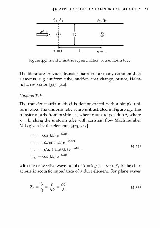
4.9 application to a cylindrical geometry 81
draft – 2014.06.17 16:06 – claus lahiri
L
D
x = 0 x = L
1 2M
p1, q1 p2, q2
Figure 4.5: Transfer matrix representation of a uniform tube.
The literature provides transfer matrices for many common ductelements, e. g. uniform tube, sudden area change, orifice, Helm-holtz resonator [323, 342].
Uniform Tube
The transfer matrix method is demonstrated with a simple uni-form tube. The uniform tube setup is illustrated in Figure 4.5. Thetransfer matrix from position 1, where x = 0, to position 2, wherex = L, along the uniform tube with constant flow Mach numberM is given by the elements [323, 343]
T11 = cos(kL) e−iMkL
T12 = iZ0 sin(kL) e−iMkL
T21 = (i/Z0) sin(kL) e−iMkL
T22 = cos(kL) e−iMkL
(4.54)
with the convective wave number k = k0/(1 − M2). Z0 is the char-acteristic acoustic impedance of a duct element. For plane waves
Z0 =p
q=
p
Av=ρc
A. (4.55)
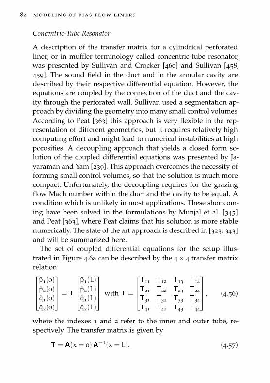
82 modeling of bias flow liners
Concentric-Tube Resonator
A description of the transfer matrix for a cylindrical perforatedliner, or in muffler terminology called concentric-tube resonator,was presented by Sullivan and Crocker [460] and Sullivan [458,459]. The sound field in the duct and in the annular cavity aredescribed by their respective differential equation. However, theequations are coupled by the connection of the duct and the cav-ity through the perforated wall. Sullivan used a segmentation ap-proach by dividing the geometry into many small control volumes.According to Peat [363] this approach is very flexible in the rep-resentation of different geometries, but it requires relatively highcomputing effort and might lead to numerical instabilities at highporosities. A decoupling approach that yields a closed form so-lution of the coupled differential equations was presented by Ja-yaraman and Yam [239]. This approach overcomes the necessity offorming small control volumes, so that the solution is much morecompact. Unfortunately, the decoupling requires for the grazingflow Mach number within the duct and the cavity to be equal. Acondition which is unlikely in most applications. These shortcom-ing have been solved in the formulations by Munjal et al. [345]and Peat [363], where Peat claims that his solution is more stablenumerically. The state of the art approach is described in [323, 343]and will be summarized here.
The set of coupled differential equations for the setup illus-trated in Figure 4.6a can be described by the 4× 4 transfer matrixrelationp1(0)p2(0)q1(0)q2(0)
= T
p1(L)
p2(L)
q1(L)
q2(L)
with T =
T11 T12 T13 T14
T21 T22 T23 T24
T31 T32 T33 T34
T41 T42 T43 T44
, (4.56)
where the indexes 1 and 2 refer to the inner and outer tube, re-spectively. The transfer matrix is given by
T = A(x = 0)A−1(x = L). (4.57)
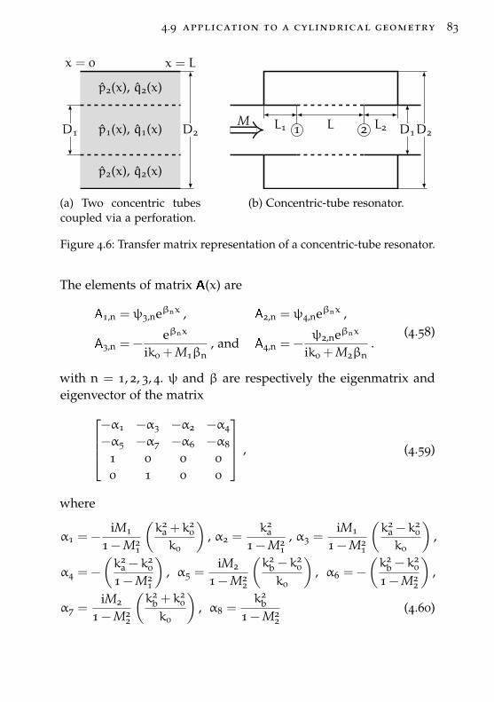
4.9 application to a cylindrical geometry 83
draft – 2014.06.17 16:06 – claus lahiri
x = 0 x = L
p2(x), q2(x)
p2(x), q2(x)
p1(x), q1(x)D1 D2
(a) Two concentric tubescoupled via a perforation.
draft – 2014.06.17 16:06 – claus lahiri
LL1 L2 D1D21 2M
(b) Concentric-tube resonator.
Figure 4.6: Transfer matrix representation of a concentric-tube resonator.
The elements of matrix A(x) are
A1,n = ψ3,neβnx , A2,n = ψ4,neβnx ,
A3,n = −eβnx
ik0 + M1βn, and A4,n = −
ψ2,neβnx
ik0 + M2βn.
(4.58)
with n = 1, 2, 3, 4. ψ and β are respectively the eigenmatrix andeigenvector of the matrix
−α1 −α3 −α2 −α4
−α5 −α7 −α6 −α8
1 0 0 00 1 0 0
, (4.59)
where
α1 = −iM1
1 − M21
(k2
a + k20
k0
), α2 =
k2a
1 − M21
, α3 =iM1
1 − M21
(k2
a − k20
k0
),
α4 = −
(k2
a − k20
1 − M21
), α5 =
iM2
1 − M22
(k2
b − k20
k0
), α6 = −
(k2
b − k20
1 − M22
),
α7 =iM2
1 − M22
(k2
b + k20
k0
), α8 =
k2b
1 − M22
(4.60)
84 modeling of bias flow liners
with
k0 =ω
c, k2
a = k20 −
4ik0
D1ζ, k2
b = k20 −
4ik0D1
(D22 −D
21) ζ
. (4.61)
and ζ is the normalized specific impedance of the perforation.All elements of the transfer matrix in Equation (4.56) can be cal-culated from Equations (4.58) to (4.61). The setup of a concentric-tube resonator, as illustrated in Figure 4.6b, introduces hard-wallboundary conditions at both ends of the cavity, so that it can berepresented by the 2× 2 transfer matrix27[
p1(0)v1(0)
]= T
[p2(L)
v2(L)
]with T =
[Ta Tb
Tc Td
](4.62)
with
Ta = T12 +A1A2 , Tb =(T14 +B1A2
)Z0
Tc =(T32 +A1B2
)/Z0 , and Td = T34 +B1B2 ,
(4.63)
where T12, T14, T32, and T34 are elements of the matrix in Equa-tion (4.56). The remaining quantities are given by
A1 =(X1T22 −T42
)/F , B1 =
(X1T24 −T44
)/F ,
A2 = T11 +X2T13 , B2 = T31 +X2T33 ,
X1 = −i tan (k0L1) , X2 = i tan (k0L2) , and
F = T41 +X2T43 −X1(T21 +X2T23
).
The transfer matrix in Equation (4.62) describes the relation ofacoustic pressure and velocity when a sound wave is travelingfrom position 1 to 2 in Figure 4.6b. The equations above includethe convective effect of a grazing flow. Commonly, there is nograzing flow within the cavity, so that M2 = 0. The acoustic be-havior of the perforation is represented by the impedance term ζ
in Equation (4.61).
27 To avoid confusion between the elements of the matrices in Equations (4.56)and (4.62), an a,b,c,d indexing scheme has been used.
4.9 application to a cylindrical geometry 85
Acoustic Performance Criteria
Traditionally, the performance of a muffler is evaluated by itstransmission loss, level difference, or insertion loss. For example,the transmission loss28 can be calculated directly from the transfermatrix elements as [323]
TL = 20 lg
(√Zn
Z1
1 + M1
1 + Mn
∣∣∣∣∣T11 +T12Zn
+T21Z1 +T22Z1Zn
2
∣∣∣∣∣)
, (4.64)
where the index 1 refers to the first and the index n to the last ele-ment of the network and the terminations are assumed anechoic.
Here, the acoustic performance is evaluated with the dissipa-tion coefficient. Therefore, the transfer matrix is converted into ascattering matrix. This is demonstrated in Appendix b.2. Then, thedissipation coefficient can be calculated from the reflection andtransmission coefficients given by the scattering matrix accordingto Section 6.4.
This method will be referred to as Transfer Matrix Method,short TMM. The acoustic properties of the liner are included inEquation (4.61) and can be represented by an impedance model ofchoice. This will be indicated, for example, by TMM:Bauer, wherethe Transfer Matrix Method is used in combination with the Bauerimpedance model.
4.9.2 Eldredge & Dowling Method
Eldredge and Dowling [142] develop equations for the stagnationenthalpy29 and the acoustic particle velocity in the lined section
28 The transmission loss describes the difference between the incident powerand transmitted power in dB, that is TL = 10 lg (Pi/Pt).
29 The fluctuating stagnation enthalpy is defined by [142, 214] B′ = p′/ρ+ vv′.For a plane wave, where the acoustic pressure and velocity are related viathe impedance ρc = p/v, the fluctuating stagnation enthalpy yields B± =pρ (1±M).
86 modeling of bias flow liners
of a duct by applying a mass and momentum balance to a de-fined control volume. An analytic solution does exist for the hard-walled duct sections upstream and downstream, so that the stag-nation enthalpy and acoustic particle velocity need to match at therespective boundaries. For convenience, they introduce the char-acteristic quantities
ψ+ =12(1 +Ug)
[B+ (1 −Ug) vx
], and (4.65)
ψ− =12(1 −Ug)
[B− (1 +Ug) vx
], (4.66)
where Ug is the grazing flow velocity and vx is the complex am-plitude of the particle velocity in axial direction within the duct.Then, the equations for the lined duct are given by
dψ+
dx= −
ikLeff
1 +Ug(x)ψ+ +
12C1Leff
Av1 and (4.67)
dψ−
dx=
ikLeff
1 −Ug(x)ψ− −
12C1Leff
Av1 , (4.68)
with the two boundary conditions
ψ+(0) = 1 and ψ−(1)e−ik−Leff −ψ+(1)reeik+Leff = 0 , (4.69)
the liner circumference C1, the effective perforation length30 Leff,the duct cross-section area A, and the acoustic particle velocitythrough the perforation v1 specified below. Please note, that thegrazing flow velocity increases with x over the length of the liner
Ug = Mg +C1Leff
AMbx . (4.70)
Eldredge and Dowling consider three configurations: 1. Open ex-terior, 2. Annular cavity enclosed by a rigid wall, and 3. Annularcavity enclosed by a second liner. Only the last two are of impor-tance here.
30 The effective perforation length yields best agreement with the experimentaldata (see the discussion in Section 4.10.2).
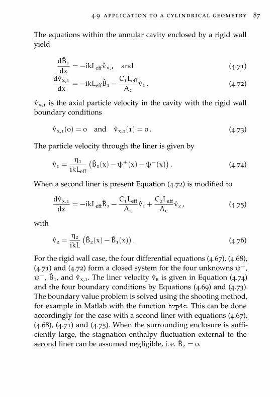
4.9 application to a cylindrical geometry 87
The equations within the annular cavity enclosed by a rigid wallyield
dB1
dx= −ikLeffvx,1 and (4.71)
dvx,1
dx= −ikLeffB1 −
C1Leff
Acv1 . (4.72)
vx,1 is the axial particle velocity in the cavity with the rigid wallboundary conditions
vx,1(0) = 0 and vx,1(1) = 0 . (4.73)
The particle velocity through the liner is given by
v1 =η1
ikLeff
(B1(x) −ψ
+(x) −ψ−(x))
. (4.74)
When a second liner is present Equation (4.72) is modified to
dvx,1
dx= −ikLeffB1 −
C1Leff
Acv1 +
C2Leff
Acv2 , (4.75)
with
v2 =η2
ikL(B2(x) − B1(x)
). (4.76)
For the rigid wall case, the four differential equations (4.67), (4.68),(4.71) and (4.72) form a closed system for the four unknowns ψ+,ψ−, B1, and vx,1. The liner velocity vb is given in Equation (4.74)and the four boundary conditions by Equations (4.69) and (4.73).The boundary value problem is solved using the shooting method,for example in Matlab with the function bvp4c. This can be doneaccordingly for the case with a second liner with equations (4.67),(4.68), (4.71) and (4.75). When the surrounding enclosure is suffi-ciently large, the stagnation enthalpy fluctuation external to thesecond liner can be assumed negligible, i. e. B2 = 0.
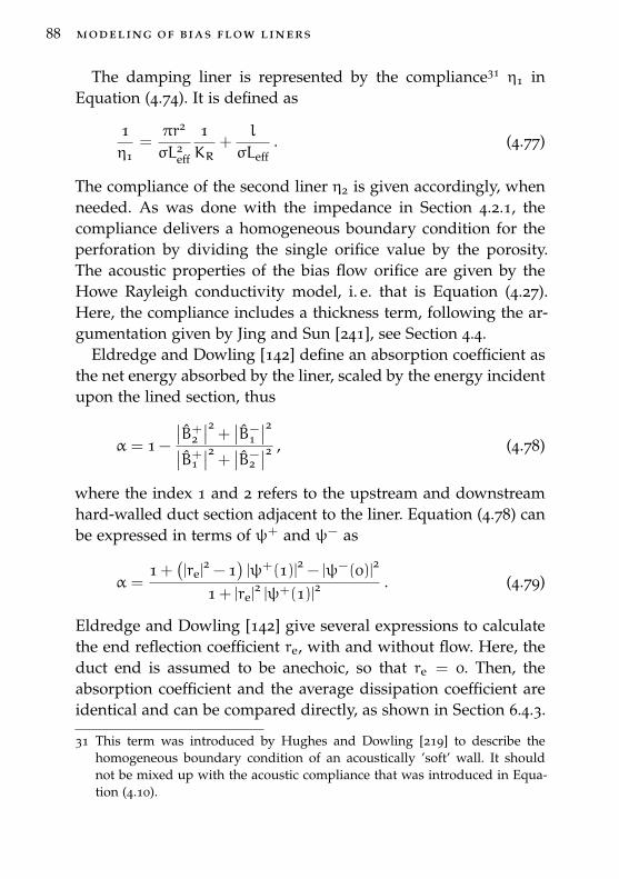
88 modeling of bias flow liners
The damping liner is represented by the compliance31 η1 inEquation (4.74). It is defined as
1η1
=πr2
σL2eff
1KR
+l
σLeff. (4.77)
The compliance of the second liner η2 is given accordingly, whenneeded. As was done with the impedance in Section 4.2.1, thecompliance delivers a homogeneous boundary condition for theperforation by dividing the single orifice value by the porosity.The acoustic properties of the bias flow orifice are given by theHowe Rayleigh conductivity model, i. e. that is Equation (4.27).Here, the compliance includes a thickness term, following the ar-gumentation given by Jing and Sun [241], see Section 4.4.
Eldredge and Dowling [142] define an absorption coefficient asthe net energy absorbed by the liner, scaled by the energy incidentupon the lined section, thus
α = 1 −
∣∣B+2∣∣2 + ∣∣B−
1∣∣2∣∣B+
1∣∣2 + ∣∣B−
2∣∣2 , (4.78)
where the index 1 and 2 refers to the upstream and downstreamhard-walled duct section adjacent to the liner. Equation (4.78) canbe expressed in terms of ψ+ and ψ− as
α =1 +
(|re|
2 − 1)|ψ+(1)|2 − |ψ−(0)|2
1 + |re|2|ψ+(1)|2
. (4.79)
Eldredge and Dowling [142] give several expressions to calculatethe end reflection coefficient re, with and without flow. Here, theduct end is assumed to be anechoic, so that re = 0. Then, theabsorption coefficient and the average dissipation coefficient areidentical and can be compared directly, as shown in Section 6.4.3.
31 This term was introduced by Hughes and Dowling [219] to describe thehomogeneous boundary condition of an acoustically ’soft’ wall. It shouldnot be mixed up with the acoustic compliance that was introduced in Equa-tion (4.10).
4.10 some comparisons 89
This approach will be referred to as Eldredge and DowlingMethod, short EDM, and EDM:Jing when including the descrip-tion of the liner according to Equation (4.77).
4.10 some comparisons
4.10.1 Impedance Models
The first comparison is done for a configuration without any flow.The linear acoustic behavior of a perforation without flow is fairlywell understood, so that the models should predict a similar be-havior. The Howe model and its derivatives are only valid whena bias flow is present, so that they are excluded from this compar-ison.
Figure 4.7 plots a) the resistance, b) the reactance, and c) thedissipation over the frequency. The liner geometry corresponds toconfiguration dc006 of the parameter study. The specifications aregiven in Table 7.1. Even without flow the impedance prediction ofthe models varies slightly. The effect of these variations on the ab-sorption are revealed in Figure 4.7c. The theoretical dissipation iscalculated with the transfer matrix method and compared to theexperimental results. Surprisingly, the oldest model, i. e. the linearMelling model, shows the best agreement with the experiments.The other models do not include some effects that are consideredin the Melling model, i. e. thermal conductivity losses within theorifice are neglected or approximations of the Bessel functions areused, for example. The prediction quality for the no flow casewould have benefited from including these effects. The peak fre-quency predicted by the Bauer model is significantly higher thanthe other models. This results from the empirical correction factorin the reactance, which is strictly valid only when a grazing flowis present (see discussion in Section 4.6).
The impedance of the same setup as above, but including a biasflow of Mb = 0.03 is plotted in Figure 4.8. The Melling model does
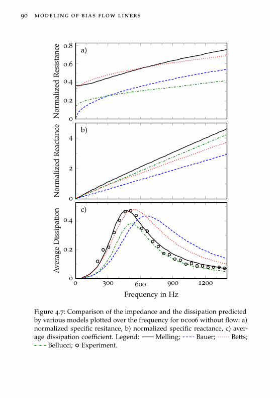
90 modeling of bias flow liners
a)
0
0.2
0.4
0.6
0.8N
orm
aliz
edR
esis
tanc
e
b)
0
2
4
Nor
mal
ized
Rea
ctan
ce
c)
0 300 600 900 12000
0.2
0.4
Frequency in Hz
Ave
rage
Dis
sipa
tion
Figure 4.7: Comparison of the impedance and the dissipation predictedby various models plotted over the frequency for dc006 without flow: a)normalized specific resitance, b) normalized specific reactance, c) aver-age dissipation coefficient. Legend: Melling; Bauer; Betts;
Bellucci; Experiment.
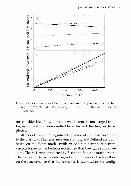
4.10 some comparisons 91
a)
3
4
5
6
Nor
mal
ized
Res
ista
nce
b)
0 300 600 900 12000
1
2
3
Frequency in Hz
Nor
mal
ized
Rea
ctan
ce
Figure 4.8: Comparison of the impedance models plotted over the fre-quency for dc006 with Mb = 0.03. Jing; Bauer; Betts;
Bellucci.
not consider bias flow, so that it would remain unchanged fromFigure 4.7 and has been omitted here. Instead, the Jing model isplotted.
All models predict a significant increase of the resistance dueto the bias flow. The resistance terms of Jing and Bellucci are bothbased on the Howe model (with an addition contribution fromviscous losses in the Bellucci model), so that they give similar re-sults. The resistance predicted by Betts and Bauer is much lower.The Betts and Bauer models neglect any influence of the bias flowon the reactance, so that the reactance is identical to the config-
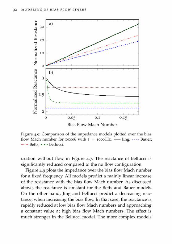
92 modeling of bias flow liners
a)
0
10
20
30
Nor
mal
ized
Res
ista
nce
b)
0 0.05 0.1 0.152
2.5
3
Bias Flow Mach Number
Nor
mal
ized
Rea
ctan
ce
Figure 4.9: Comparison of the impedance models plotted over the biasflow Mach number for dc006 with f = 1000 Hz. Jing; Bauer;
Betts; Bellucci.
uration without flow in Figure 4.7. The reactance of Bellucci issignificantly reduced compared to the no flow configuration.
Figure 4.9 plots the impedance over the bias flow Mach numberfor a fixed frequency. All models predict a mainly linear increaseof the resistance with the bias flow Mach number. As discussedabove, the reactance is constant for the Betts and Bauer models.On the other hand, Jing and Bellucci predict a decreasing reac-tance, when increasing the bias flow. In that case, the reactance israpidly reduced at low bias flow Mach numbers and approachinga constant value at high bias flow Mach numbers. The effect ismuch stronger in the Bellucci model. The more complex models
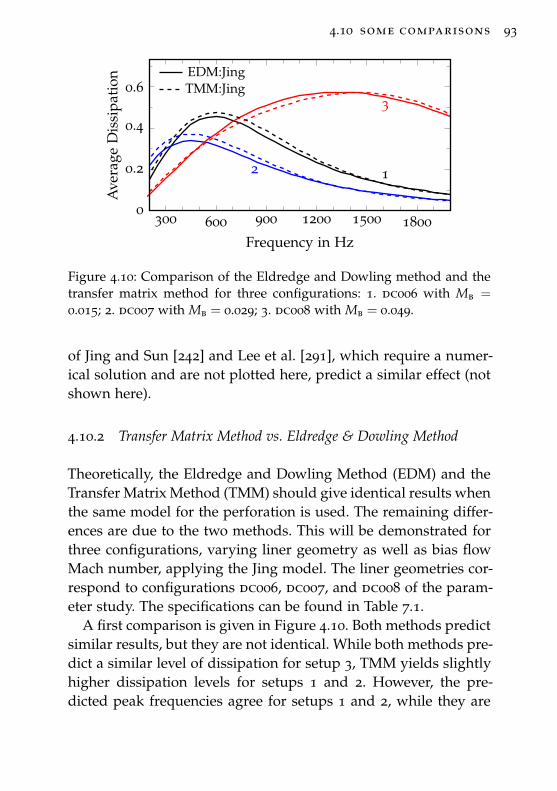
4.10 some comparisons 93
12
3
300 600 900 1200 1500 18000
0.2
0.4
0.6
Frequency in Hz
Ave
rage
Dis
sipa
tion
EDM:JingTMM:Jing
Figure 4.10: Comparison of the Eldredge and Dowling method and thetransfer matrix method for three configurations: 1. dc006 with Mb =
0.015; 2. dc007 with Mb = 0.029; 3. dc008 with Mb = 0.049.
of Jing and Sun [242] and Lee et al. [291], which require a numer-ical solution and are not plotted here, predict a similar effect (notshown here).
4.10.2 Transfer Matrix Method vs. Eldredge & Dowling Method
Theoretically, the Eldredge and Dowling Method (EDM) and theTransfer Matrix Method (TMM) should give identical results whenthe same model for the perforation is used. The remaining differ-ences are due to the two methods. This will be demonstrated forthree configurations, varying liner geometry as well as bias flowMach number, applying the Jing model. The liner geometries cor-respond to configurations dc006, dc007, and dc008 of the param-eter study. The specifications can be found in Table 7.1.
A first comparison is given in Figure 4.10. Both methods predictsimilar results, but they are not identical. While both methods pre-dict a similar level of dissipation for setup 3, TMM yields slightlyhigher dissipation levels for setups 1 and 2. However, the pre-dicted peak frequencies agree for setups 1 and 2, while they are
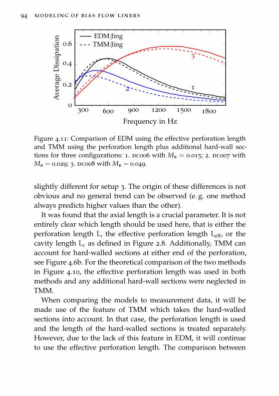
94 modeling of bias flow liners
12
3
300 600 900 1200 1500 18000
0.2
0.4
0.6
Frequency in Hz
Ave
rage
Dis
sipa
tion
EDM:JingTMM:Jing
Figure 4.11: Comparison of EDM using the effective perforation lengthand TMM using the perforation length plus additional hard-wall sec-tions for three configurations: 1. dc006 with Mb = 0.015; 2. dc007 withMb = 0.029; 3. dc008 with Mb = 0.049.
slightly different for setup 3. The origin of these differences is notobvious and no general trend can be observed (e. g. one methodalways predicts higher values than the other).
It was found that the axial length is a crucial parameter. It is notentirely clear which length should be used here, that is either theperforation length L, the effective perforation length Leff, or thecavity length Lc as defined in Figure 2.8. Additionally, TMM canaccount for hard-walled sections at either end of the perforation,see Figure 4.6b. For the theoretical comparison of the two methodsin Figure 4.10, the effective perforation length was used in bothmethods and any additional hard-wall sections were neglected inTMM.
When comparing the models to measurement data, it will bemade use of the feature of TMM which takes the hard-walledsections into account. In that case, the perforation length is usedand the length of the hard-walled sections is treated separately.However, due to the lack of this feature in EDM, it will continueto use the effective perforation length. The comparison between
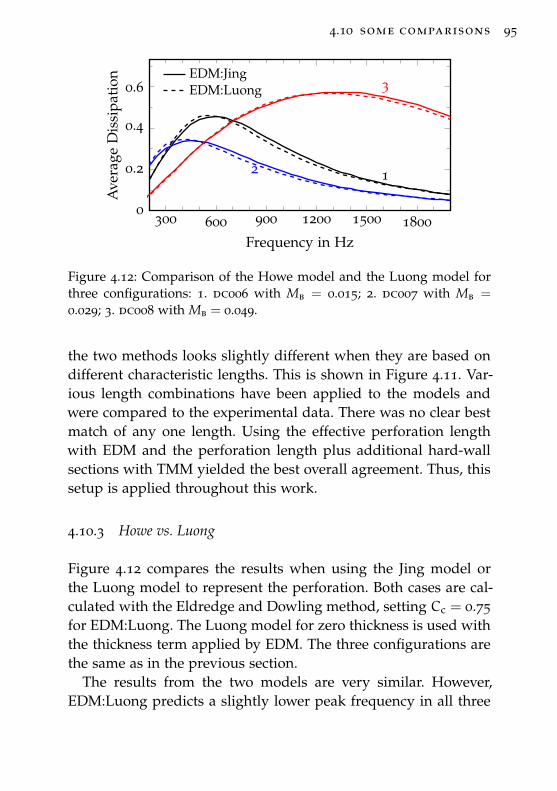
4.10 some comparisons 95
300 600 900 1200 1500 18000
0.2
0.4
0.6
12
3
Frequency in Hz
Ave
rage
Dis
sipa
tion
EDM:JingEDM:Luong
Figure 4.12: Comparison of the Howe model and the Luong model forthree configurations: 1. dc006 with Mb = 0.015; 2. dc007 with Mb =
0.029; 3. dc008 with Mb = 0.049.
the two methods looks slightly different when they are based ondifferent characteristic lengths. This is shown in Figure 4.11. Var-ious length combinations have been applied to the models andwere compared to the experimental data. There was no clear bestmatch of any one length. Using the effective perforation lengthwith EDM and the perforation length plus additional hard-wallsections with TMM yielded the best overall agreement. Thus, thissetup is applied throughout this work.
4.10.3 Howe vs. Luong
Figure 4.12 compares the results when using the Jing model orthe Luong model to represent the perforation. Both cases are cal-culated with the Eldredge and Dowling method, setting Cc = 0.75for EDM:Luong. The Luong model for zero thickness is used withthe thickness term applied by EDM. The three configurations arethe same as in the previous section.
The results from the two models are very similar. However,EDM:Luong predicts a slightly lower peak frequency in all three
96 modeling of bias flow liners
cases. Due to their similar results, only EDM:Jing will be com-pared with the experimental data in Chapter 7.
5D U C T A C O U S T I C S
5.1 acoustic wave equation
Fundamental Equations of Fluid Dynamics
The motion of fluid is governed by the conservation laws formass, momentum, and energy. The conservation of mass in theabsence of any sources is described by the partial differential equa-tion1 (Euler [148], or [33, 369])
∂ρ
∂t+∇ · (ρv) = 0 . (5.1)
It is commonly known as the continuity equation. It relates thevelocity of the fluid to its density and is valid without any restric-tions, except that the fluid and its properties must be continuous2.An alternative formulation is given by replacing the local timederivative ∂/∂t with the substantial derivative (Stokes [449], or[33, 59])
D
Dt=∂
∂t+ v∇ . (5.2)
1 This and the following equations are given in Gibbs notation (Gibbs and Wil-son [173], or [59]). The Nabla operator ∇ is used as a convenient mathemati-cal notation for either the gradient grad f = ∇f, the divergence div f = ∇ · f,or rotation (or curl) rot f = ∇× f [77].
2 The continuum hypothesis disregards the discrete molecular nature of a fluidand assumes, that its macroscopic behavior is the same as if it were perfectlycontinuous in structure [33].
98 duct acoustics
The substantial time derivative follows the motion of the fluid,thus it reveals the convective effect of the mean flow. It followsfrom Equation (5.1) that [33]
Dρ
Dt+ ρ (∇ · v) = 0 . (5.3a)
The conservation of momentum for an ideal fluid is given by (Eu-ler [148] or [33, 369])
ρDvDt
= −∇p , (5.3b)
where gravity is neglected. This equation is also called equationof motion, while this special case for an ideal fluid is commonlyknown as the Euler equation3. It relates the pressure to the veloc-ity of the fluid.
The conservation of energy is expressed by the equation of state,which for an ideal gas4 is given by (Clapeyron [97], or [33])
p = ρRT .
This equation is also called ideal gas law. The acoustic motion isconsidered to be isentropic5, so that the thermodynamic relationbetween the density and the pressure can be given by [33, 369](
∂p
∂ρ
)s
= c2 withDs
Dt= 0 . (5.3c)
This system of three Equations (5.3) is commonly referred to as Eu-ler equations6. They describe the motion of a compressible, idealfluid.
3 Named after Leonhard Euler (1707-1783), Swiss mathematician and physi-cist.
4 An ideal gas is an idealization where the molecular interaction is neglected.Air of normal atmospheric temperature and pressure can be considered tobehave ideal.
5 Morfey [338]: “In an isentropic change of thermodynamic state the entropyremains constant. An adiabatic process is isentropic provided it is reversible.”
6 Even though only the first two originate from Euler.
5.1 acoustic wave equation 99
Equations of Linear Acoustics
The field quantities (pressure, velocity, and density) that are usedin the previous section can be written as the sum of their meanand fluctuating (acoustic) values:
p = p0 + p′
v = v0 + v′
ρ = ρ0 + ρ′
(5.4)
A linearization of Equations (5.3) is possible by assuming that theacoustic quantities are much smaller than the mean quantities
p′
p0� 1
v′
v0� 1
ρ′
ρ0� 1 , (5.5)
which is fulfilled in most applications. This assumption allowsto disregard higher order terms in Equations (5.3), so that theapproximate acoustic equations are given by [176, 369]
Dρ′
Dt+ ρ0
(∇ · v′
)= 0 , (5.6a)
ρ0Dv′
Dt+∇p′ = 0 , and (5.6b)
p′ = c2ρ′ . (5.6c)
Acoustic Wave Equation
The acoustic wave equation can be obtained from Equation (5.6)in a few simple steps: Substitute the fluctuating density ρ′ inEquation (5.6a) with (5.6c). Then, taking the time derivative ofEquation (5.6a) and replacing its second term with Equation (5.6b)yields the acoustic wave equation
∇2p′ −1c2D2p′
Dt2= 0 . (5.7)
100 duct acoustics
where ∇2 is the Laplace operator7. This general notation includ-ing the material derivative, see Equation (5.2), can be applied tostationary or moving medium. The assumptions that have beenintroduced are:
• homogeneous medium8
• ideal fluid
• linear acoustics9
• isentropic relation between pressure and density
• uniform flow10 or stationary medium
Expanding the material derivative in Equation (5.7) results in thecommonly used form of the convected wave equation (Howe [207,214], or [340, 343])
∇2p′ −1c2
(∂
∂t+ v0∇
)2
p′ = 0 . (5.8)
In stationary medium, v0 = 0, the material derivative can be re-placed by the local time derivative and Equation (5.7) and ((5.8))reduce to the well known form of the classical acoustic wave equa-tion (d’Alembert [111] and Euler [149, 150], or [369])
∇2p′ −1c2∂2p′
∂t2= 0 . (5.9)
7 The Laplace operator ∇2, or sometimes denoted as ∆, is named after Pierre-Simon de Laplace (1749–1827, French mathematician). It prescribes the sum-mation of the second partial derivatives of a function f with respect to agiven coordinate system. In general: ∇2f = ∇ · (∇f) = div(grad f) [77]
8 Morfey [338]: “A homogeneous medium is a medium whose properties arespatially uniform, i.e. independent of position.”
9 Morfey [338]: “Linear acoustics is limited to small amplitude signals or os-cillations, so that the relation between any two oscillatory quantities is inde-pendent of amplitude. Linear sound waves propagate independently of oneanother, without interaction.”
10 In uniform flow the magnitude and direction of the velocity is spatially uni-form.
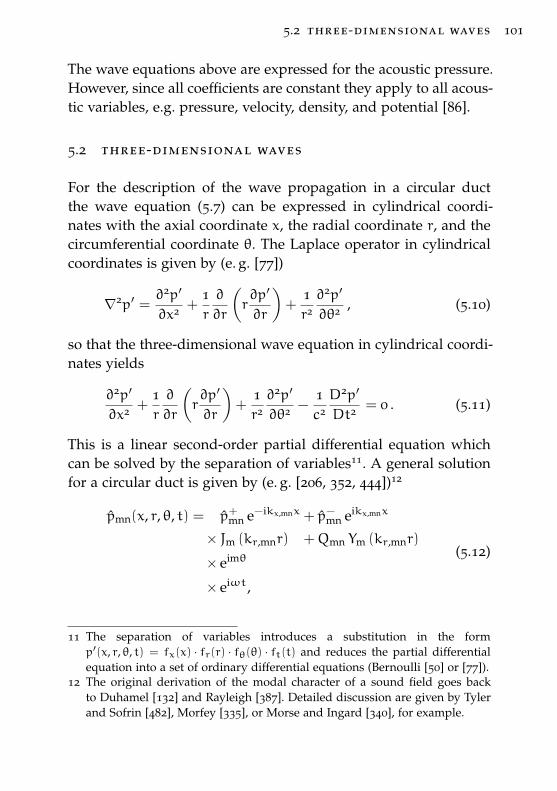
5.2 three-dimensional waves 101
The wave equations above are expressed for the acoustic pressure.However, since all coefficients are constant they apply to all acous-tic variables, e.g. pressure, velocity, density, and potential [86].
5.2 three-dimensional waves
For the description of the wave propagation in a circular ductthe wave equation (5.7) can be expressed in cylindrical coordi-nates with the axial coordinate x, the radial coordinate r, and thecircumferential coordinate θ. The Laplace operator in cylindricalcoordinates is given by (e. g. [77])
∇2p′ =∂2p′
∂x2 +1r
∂
∂r
(r∂p′
∂r
)+
1r2∂2p′
∂θ2 , (5.10)
so that the three-dimensional wave equation in cylindrical coordi-nates yields
∂2p′
∂x2 +1r
∂
∂r
(r∂p′
∂r
)+
1r2∂2p′
∂θ2 −1c2D2p′
Dt2= 0 . (5.11)
This is a linear second-order partial differential equation whichcan be solved by the separation of variables11. A general solutionfor a circular duct is given by (e. g. [206, 352, 444])12
pmn(x, r, θ, t) = p+mn e−ikx,mnx + p−mn eikx,mnx
× Jm (kr,mnr) +Qmn Ym (kr,mnr)
× eimθ
× eiωt,
(5.12)
11 The separation of variables introduces a substitution in the formp′(x, r, θ, t) = fx(x) · fr(r) · fθ(θ) · ft(t) and reduces the partial differentialequation into a set of ordinary differential equations (Bernoulli [50] or [77]).
12 The original derivation of the modal character of a sound field goes backto Duhamel [132] and Rayleigh [387]. Detailed discussion are given by Tylerand Sofrin [482], Morfey [335], or Morse and Ingard [340], for example.

102 duct acoustics
where the axial and radial wave numbers are related by(ωc
)2= k2
x,mn + k2r,mn. (5.13)
The four rows in Equation (5.12) describe the spatial (axial, radial,and circumferential) and temporal shape of the mode, respectively.While the spatial patterns in axial and circumferential directionare sinusoidal (as well as the temporal development), the radialpattern is defined by Bessel functions. Jm is the Bessel functionof the first kind, commonly only called Bessel function, Ym is theBessel function of the second kind, often called Weber13 or Neu-mann14 function, and Qmn is the n-th Eigenvalue of Ym.
Equation (5.12) represents the so called modal solution. The ac-tual sound pressure of a time harmonic wave is given by the realpart of the superposition of an infinite number of modes15
p′(x, r, θ, t) =∑m
∑n
pmn(x, r, θ, t) , (5.14)
where m ∈ {. . . ,−2,−1, 0, 1, 2, . . . } and n ∈ {0, 1, 2, . . . }. Each modeis characterized by its circumferential mode order m and its radialmode order n. The integers m and n describe the number of nodallines in circumferential and radial direction, respectively. For m =
0 and n = 0 there are no nodal lines in transverse direction, so thatthe sound field is one-dimensional with variations in x-directiononly. This special case is called fundamental mode or plane waveand will be discussed separately in Section 5.3. All other modesare referred to as higher order modes.
In a cylindrical duct, without any central hub, Qmn in Equa-tion (5.12) becomes zero, so that the solution for a time harmonic
13 Named after Heinrich Martin Weber (1842-1913, German mathematician).14 Named after Carl Gottfried Neumann (1832-1925, German mathematician).15 Morfey [338]: “A mode is a spatial pattern of vibration, whose shape remains
invariant as the vibration propagates spatially.”
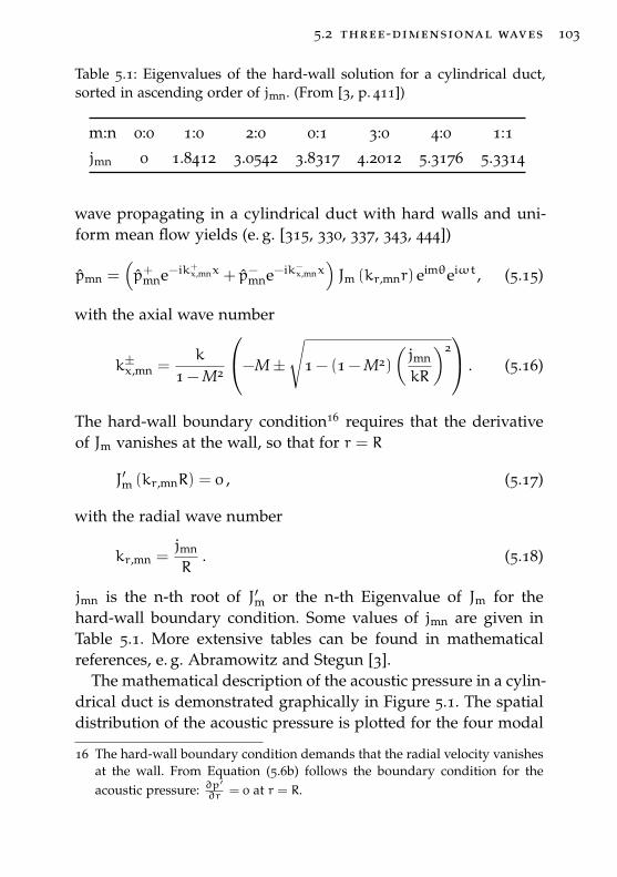
5.2 three-dimensional waves 103
Table 5.1: Eigenvalues of the hard-wall solution for a cylindrical duct,sorted in ascending order of jmn. (From [3, p. 411])
m:n 0:0 1:0 2:0 0:1 3:0 4:0 1:1
jmn 0 1.8412 3.0542 3.8317 4.2012 5.3176 5.3314
wave propagating in a cylindrical duct with hard walls and uni-form mean flow yields (e. g. [315, 330, 337, 343, 444])
pmn =(p+mne−ik+x,mnx + p−mne−ik−x,mnx
)Jm (kr,mnr) eimθeiωt, (5.15)
with the axial wave number
k±x,mn =k
1 − M2
−M±√
1 − (1 − M2)
(jmn
kR
)2 . (5.16)
The hard-wall boundary condition16 requires that the derivativeof Jm vanishes at the wall, so that for r = R
J′m (kr,mnR) = 0 , (5.17)
with the radial wave number
kr,mn =jmn
R. (5.18)
jmn is the n-th root of J′m or the n-th Eigenvalue of Jm for thehard-wall boundary condition. Some values of jmn are given inTable 5.1. More extensive tables can be found in mathematicalreferences, e. g. Abramowitz and Stegun [3].
The mathematical description of the acoustic pressure in a cylin-drical duct is demonstrated graphically in Figure 5.1. The spatialdistribution of the acoustic pressure is plotted for the four modal
16 The hard-wall boundary condition demands that the radial velocity vanishesat the wall. From Equation (5.6b) follows the boundary condition for theacoustic pressure: ∂p
′
∂r = 0 at r = R.
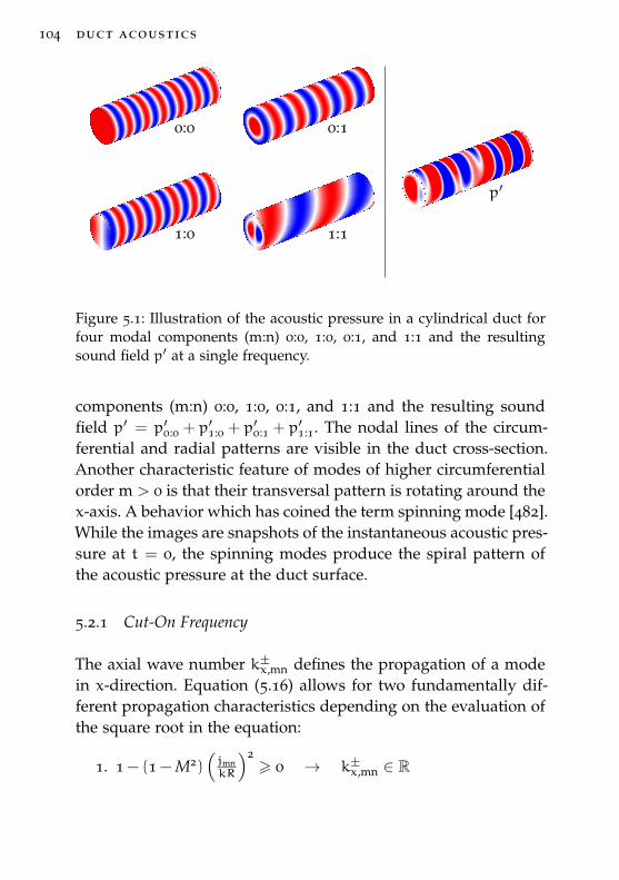
104 duct acoustics
draft – 2014.06.17 16:08 – claus lahiri
0:0
draft – 2014.06.17 16:08 – claus lahiri
0:1
draft – 2014.06.17 16:08 – claus lahiri
p′
draft – 2014.06.17 16:08 – claus lahiri
1:0
draft – 2014.06.17 16:08 – claus lahiri
1:1
Figure 5.1: Illustration of the acoustic pressure in a cylindrical duct forfour modal components (m:n) 0:0, 1:0, 0:1, and 1:1 and the resultingsound field p′ at a single frequency.
components (m:n) 0:0, 1:0, 0:1, and 1:1 and the resulting soundfield p′ = p′0:0 + p
′1:0 + p
′0:1 + p
′1:1. The nodal lines of the circum-
ferential and radial patterns are visible in the duct cross-section.Another characteristic feature of modes of higher circumferentialorder m > 0 is that their transversal pattern is rotating around thex-axis. A behavior which has coined the term spinning mode [482].While the images are snapshots of the instantaneous acoustic pres-sure at t = 0, the spinning modes produce the spiral pattern ofthe acoustic pressure at the duct surface.
5.2.1 Cut-On Frequency
The axial wave number k±x,mn defines the propagation of a modein x-direction. Equation (5.16) allows for two fundamentally dif-ferent propagation characteristics depending on the evaluation ofthe square root in the equation:
1. 1 − (1 − M2)(jmnkR
)2> 0 → k±x,mn ∈ R
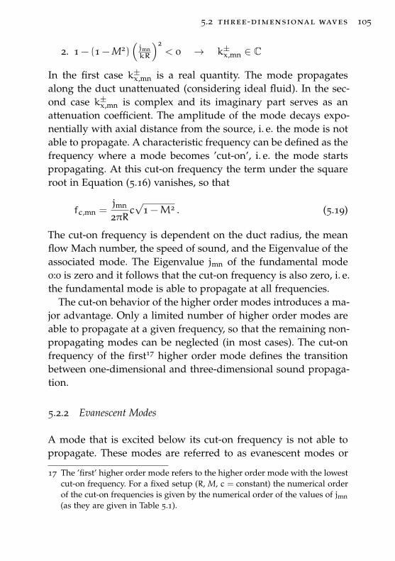
5.2 three-dimensional waves 105
2. 1 − (1 − M2)(jmnkR
)2< 0 → k±x,mn ∈ C
In the first case k±x,mn is a real quantity. The mode propagatesalong the duct unattenuated (considering ideal fluid). In the sec-ond case k±x,mn is complex and its imaginary part serves as anattenuation coefficient. The amplitude of the mode decays expo-nentially with axial distance from the source, i. e. the mode is notable to propagate. A characteristic frequency can be defined as thefrequency where a mode becomes ’cut-on’, i. e. the mode startspropagating. At this cut-on frequency the term under the squareroot in Equation (5.16) vanishes, so that
fc,mn =jmn
2πRc√
1 −M2 . (5.19)
The cut-on frequency is dependent on the duct radius, the meanflow Mach number, the speed of sound, and the Eigenvalue of theassociated mode. The Eigenvalue jmn of the fundamental mode0:0 is zero and it follows that the cut-on frequency is also zero, i. e.the fundamental mode is able to propagate at all frequencies.
The cut-on behavior of the higher order modes introduces a ma-jor advantage. Only a limited number of higher order modes areable to propagate at a given frequency, so that the remaining non-propagating modes can be neglected (in most cases). The cut-onfrequency of the first17 higher order mode defines the transitionbetween one-dimensional and three-dimensional sound propaga-tion.
5.2.2 Evanescent Modes
A mode that is excited below its cut-on frequency is not able topropagate. These modes are referred to as evanescent modes or
17 The ’first’ higher order mode refers to the higher order mode with the lowestcut-on frequency. For a fixed setup (R, M, c = constant) the numerical orderof the cut-on frequencies is given by the numerical order of the values of jmn(as they are given in Table 5.1).
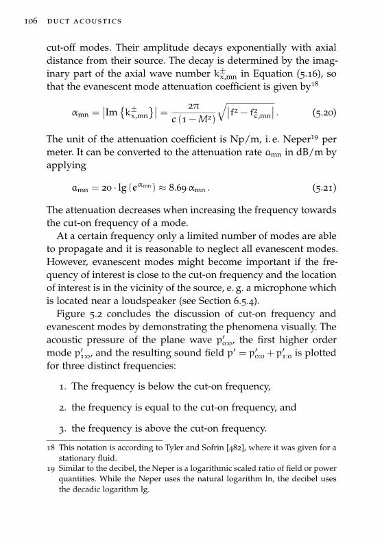
106 duct acoustics
cut-off modes. Their amplitude decays exponentially with axialdistance from their source. The decay is determined by the imag-inary part of the axial wave number k±x,mn in Equation (5.16), sothat the evanescent mode attenuation coefficient is given by18
αmn =∣∣Im{k±x,mn
}∣∣ = 2πc (1 − M2)
√∣∣f2 − f2c,mn
∣∣ . (5.20)
The unit of the attenuation coefficient is Np/m, i. e. Neper19 permeter. It can be converted to the attenuation rate amn in dB/m byapplying
amn = 20 · lg (eαmn) ≈ 8.69αmn . (5.21)
The attenuation decreases when increasing the frequency towardsthe cut-on frequency of a mode.
At a certain frequency only a limited number of modes are ableto propagate and it is reasonable to neglect all evanescent modes.However, evanescent modes might become important if the fre-quency of interest is close to the cut-on frequency and the locationof interest is in the vicinity of the source, e. g. a microphone whichis located near a loudspeaker (see Section 6.5.4).
Figure 5.2 concludes the discussion of cut-on frequency andevanescent modes by demonstrating the phenomena visually. Theacoustic pressure of the plane wave p′0:0, the first higher ordermode p′1:0, and the resulting sound field p′ = p′0:0 + p′1:0 is plottedfor three distinct frequencies:
1. The frequency is below the cut-on frequency,
2. the frequency is equal to the cut-on frequency, and
3. the frequency is above the cut-on frequency.
18 This notation is according to Tyler and Sofrin [482], where it was given for astationary fluid.
19 Similar to the decibel, the Neper is a logarithmic scaled ratio of field or powerquantities. While the Neper uses the natural logarithm ln, the decibel usesthe decadic logarithm lg.
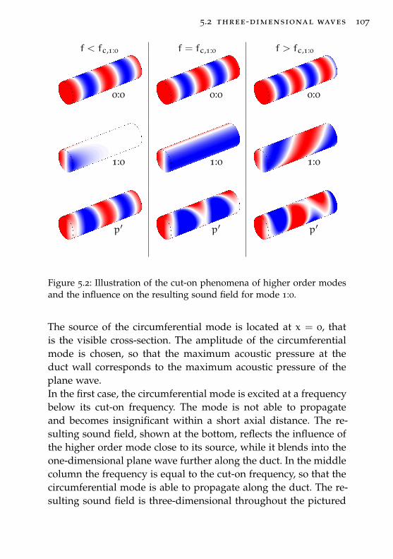
5.2 three-dimensional waves 107
f < fc,1:0 f = fc,1:0 f > fc,1:0
draft – 2014.06.17 16:08 – claus lahiri
0:0
draft – 2014.06.17 16:09 – claus lahiri
0:0
draft – 2014.06.17 16:09 – claus lahiri
0:0
draft – 2014.06.17 16:09 – claus lahiri
1:0
draft – 2014.06.17 16:09 – claus lahiri
1:0
draft – 2014.06.17 16:09 – claus lahiri
1:0
draft – 2014.06.17 16:09 – claus lahiri
p′
draft – 2014.06.17 16:10 – claus lahiri
p′
draft – 2014.06.17 16:10 – claus lahiri
p′
Figure 5.2: Illustration of the cut-on phenomena of higher order modesand the influence on the resulting sound field for mode 1:0.
The source of the circumferential mode is located at x = 0, thatis the visible cross-section. The amplitude of the circumferentialmode is chosen, so that the maximum acoustic pressure at theduct wall corresponds to the maximum acoustic pressure of theplane wave.In the first case, the circumferential mode is excited at a frequencybelow its cut-on frequency. The mode is not able to propagateand becomes insignificant within a short axial distance. The re-sulting sound field, shown at the bottom, reflects the influence ofthe higher order mode close to its source, while it blends into theone-dimensional plane wave further along the duct. In the middlecolumn the frequency is equal to the cut-on frequency, so that thecircumferential mode is able to propagate along the duct. The re-sulting sound field is three-dimensional throughout the pictured
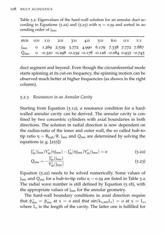
108 duct acoustics
Table 5.2: Eigenvalues of the hard-wall solution for an annular duct ac-cording to Equations (5.22) and (5.23) with η = 0.59 and sorted in as-cending order of jmn.
m:n 0:0 1:0 2:0 3:0 4:0 5:0 6:0 0:1 1:1
jmn 0 1.269 2.529 3.772 4.990 6.179 7.338 7.772 7.887Qmn 0 -0.320 -0.298 -0.239 -0.178 -0.126 -0.084 0.935 -0.745
duct segment and beyond. Even though the circumferential modestarts spinning at its cut-on frequency, the spinning motion can beobserved much better at higher frequencies (as shown in the rightcolumn).
5.2.3 Resonances in an Annular Cavity
Starting from Equation (5.12), a resonance condition for a hard-walled annular cavity can be derived. The annular cavity is con-fined by two concentric cylinders with axial boundaries in bothdirections. The solution in radial direction is now dependent onthe radius-ratio of the inner and outer wall, the so called hub-to-tip ratio η = Rhub/R. jmn and Qmn are determined by solving theequations (e. g. [255])
J ′m(jmn)Y′m(ηjmn) − J
′m(ηjmn)Y
′m(jmn) = 0 (5.22)
Qmn = −J ′m(jmn)
Y ′m(jmn)(5.23)
Equation (5.22) needs to be solved numerically. Some values ofjmn and Qmn for a hub-to-tip ratio η = 0.59 are listed in Table 5.2.The radial wave number is still defined by Equation (5.18), withthe appropriate values of jmn for the annular geometry.
The hard-wall boundary conditions in axial direction requirethat p+mn = p−mn at x = 0 and that sin(kx,mnLc) = 0 at x = Lc,where Lc is the length of the cavity. The latter one is fulfilled for
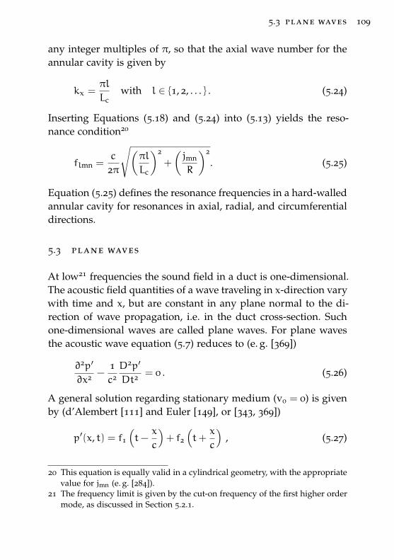
5.3 plane waves 109
any integer multiples of π, so that the axial wave number for theannular cavity is given by
kx =πl
Lcwith l ∈ {1, 2, . . . } . (5.24)
Inserting Equations (5.18) and (5.24) into (5.13) yields the reso-nance condition20
flmn =c
2π
√(πl
Lc
)2
+
(jmn
R
)2
. (5.25)
Equation (5.25) defines the resonance frequencies in a hard-walledannular cavity for resonances in axial, radial, and circumferentialdirections.
5.3 plane waves
At low21 frequencies the sound field in a duct is one-dimensional.The acoustic field quantities of a wave traveling in x-direction varywith time and x, but are constant in any plane normal to the di-rection of wave propagation, i.e. in the duct cross-section. Suchone-dimensional waves are called plane waves. For plane wavesthe acoustic wave equation (5.7) reduces to (e. g. [369])
∂2p′
∂x2 −1c2D2p′
Dt2= 0 . (5.26)
A general solution regarding stationary medium (v0 = 0) is givenby (d’Alembert [111] and Euler [149], or [343, 369])
p′(x, t) = f1
(t−
x
c
)+ f2
(t+
x
c
), (5.27)
20 This equation is equally valid in a cylindrical geometry, with the appropriatevalue for jmn (e. g. [284]).
21 The frequency limit is given by the cut-on frequency of the first higher ordermode, as discussed in Section 5.2.1.
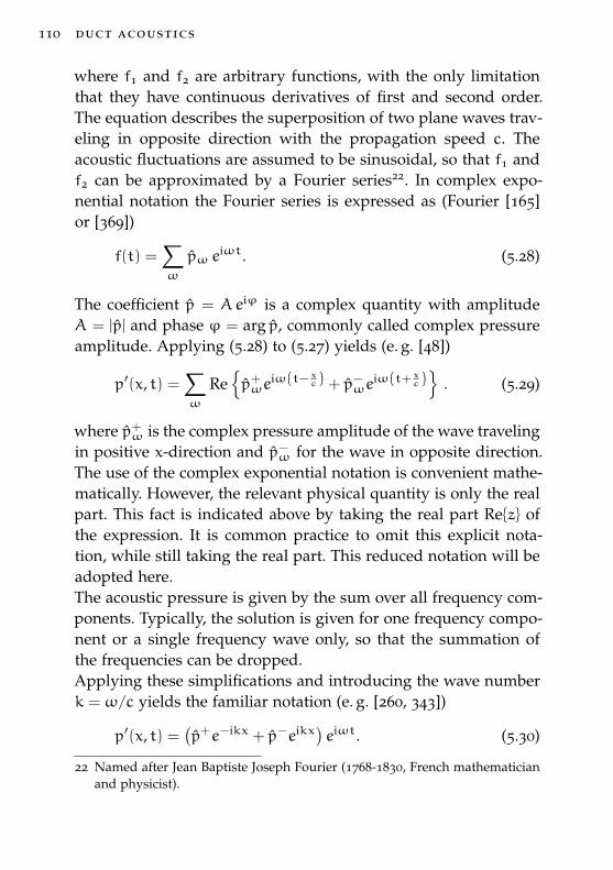
110 duct acoustics
where f1 and f2 are arbitrary functions, with the only limitationthat they have continuous derivatives of first and second order.The equation describes the superposition of two plane waves trav-eling in opposite direction with the propagation speed c. Theacoustic fluctuations are assumed to be sinusoidal, so that f1 andf2 can be approximated by a Fourier series22. In complex expo-nential notation the Fourier series is expressed as (Fourier [165]or [369])
f(t) =∑ω
pω eiωt. (5.28)
The coefficient p = Aeiϕ is a complex quantity with amplitudeA = |p| and phase ϕ = arg p, commonly called complex pressureamplitude. Applying (5.28) to (5.27) yields (e. g. [48])
p′(x, t) =∑ω
Re{p+ωe
iω(t− xc ) + p−ωe
iω(t+ xc )}
. (5.29)
where p+ω is the complex pressure amplitude of the wave travelingin positive x-direction and p−ω for the wave in opposite direction.The use of the complex exponential notation is convenient mathe-matically. However, the relevant physical quantity is only the realpart. This fact is indicated above by taking the real part Re{z} ofthe expression. It is common practice to omit this explicit nota-tion, while still taking the real part. This reduced notation will beadopted here.The acoustic pressure is given by the sum over all frequency com-ponents. Typically, the solution is given for one frequency compo-nent or a single frequency wave only, so that the summation ofthe frequencies can be dropped.Applying these simplifications and introducing the wave numberk = ω/c yields the familiar notation (e. g. [260, 343])
p′(x, t) =(p+e−ikx + p−eikx) eiωt. (5.30)
22 Named after Jean Baptiste Joseph Fourier (1768-1830, French mathematicianand physicist).
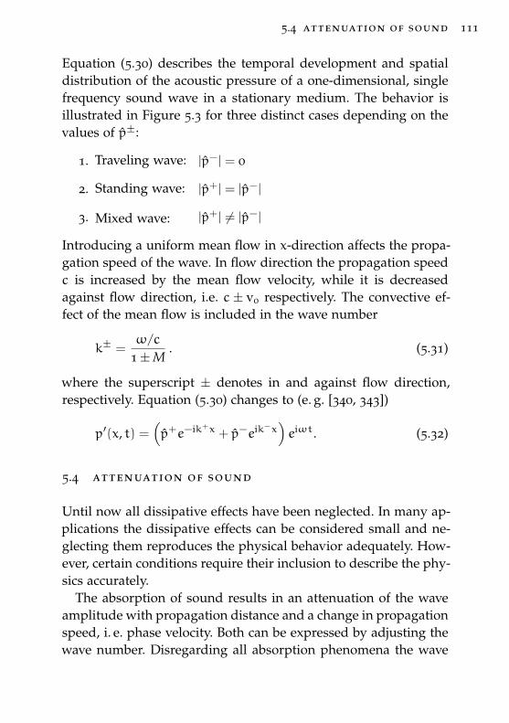
5.4 attenuation of sound 111
Equation (5.30) describes the temporal development and spatialdistribution of the acoustic pressure of a one-dimensional, singlefrequency sound wave in a stationary medium. The behavior isillustrated in Figure 5.3 for three distinct cases depending on thevalues of p±:
1. Traveling wave: |p−| = 0
2. Standing wave: |p+| = |p−|
3. Mixed wave: |p+| 6= |p−|
Introducing a uniform mean flow in x-direction affects the propa-gation speed of the wave. In flow direction the propagation speedc is increased by the mean flow velocity, while it is decreasedagainst flow direction, i.e. c± v0 respectively. The convective ef-fect of the mean flow is included in the wave number
k± =ω/c
1±M. (5.31)
where the superscript ± denotes in and against flow direction,respectively. Equation (5.30) changes to (e. g. [340, 343])
p′(x, t) =(p+e−ik+x + p−eik−x
)eiωt. (5.32)
5.4 attenuation of sound
Until now all dissipative effects have been neglected. In many ap-plications the dissipative effects can be considered small and ne-glecting them reproduces the physical behavior adequately. How-ever, certain conditions require their inclusion to describe the phy-sics accurately.
The absorption of sound results in an attenuation of the waveamplitude with propagation distance and a change in propagationspeed, i. e. phase velocity. Both can be expressed by adjusting thewave number. Disregarding all absorption phenomena the wave
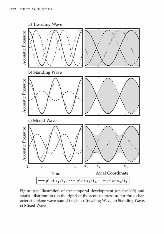
112 duct acoustics
Aco
usti
cPr
essu
reA
cous
tic
Pres
sure
t1 t2 t3
Time
Aco
usti
cPr
essu
re
x1 x2 x3
Axial Coordinate
a) Traveling Wave
b) Standing Wave
c) Mixed Wave
p′ at x1/t1, p′ at x2/t2, p′ at x3/t3
Figure 5.3: Illustration of the temporal development (on the left) andspatial distribution (on the right) of the acoustic pressure for three char-acteristic plane wave sound fields: a) Traveling Wave, b) Standing Wave,c) Mixed Wave.
5.4 attenuation of sound 113
number is real and given by k0 = ω/c (in a stationary medium).Including absorption the wave number becomes a complex quan-tity, while Equation (5.30) remains unchanged
p′(x, t) =(p+e−ikx + p−eikx) eiωt with k =
ω
cph− iα , (5.33)
where α = −Im{k} is the attenuation coefficient in Np/m andcph = ω/Re{k} is the phase velocity in m/s.The attenuation coefficient accounts for the amplitude attenuation.Without any absorption α = 0. The attenuation rate a in unitsdB/m can be computed according to Equation (5.21). The phasevelocity reflects a possible change in propagation speed. Whencph is a function of the frequency, the propagation is dispersive,i. e. waves of different frequencies propagate at different speeds.Disregarding any absorption cph = c and the propagation is non-dispersive.
Some authors prefer the formulation with the propagation con-stant Γ instead of the wave number. Confusingly, there are someslightly different notations in use. Defined in ISO 80000-8:2007[235] the propagation constant is related to the wave number byΓ = ik, so that (e. g. [257, 492, 508])
p ′ =(p+e−Γx + p−eΓx
)eiωt with Γ = α+ i
ω
cph, (5.34)
where α = Re{Γ }, cph = ω/Im{Γ }, and k = Γ/i. However, anothercommon notation seems to be (e. g. [359, 405, 475, 498])
p ′ =(p+e−k0Γx + p−ek0Γx
)eiωt with Γ =
α
k0+ i
c
cph, (5.35)
where α = k0Re{Γ }, cph = c/Im{Γ }, and k = k0Γ/i. Yet anothernotation can be found in [126–128]23
p ′ =(p+e−ik0Γx + p−eik0Γx
)eiωt with Γ =
c
cph− iα
k0, (5.36)
23 Unlike here, the references include the sign of the exponent ik0Γ in the prop-agation constant Γ .
114 duct acoustics
where α = −k0Im{Γ }, cph = c/Re{Γ }, and k = k0Γ . These differ-ences should be kept in mind when browsing the literature. Here,the wave number notation as in Equation (5.33) will be used.
5.4.1 Losses at the Wall
Historically, the effect of viscosity on sound propagation has beenstudied by Stokes [451] and von Helmholtz [195]. Inspired by theexperiments of Kundt [273], Kirchhoff [261] included the thermalconductivity losses and presented a theoretical description of thesound propagation including viscosity and thermal conductivity.His result is still the state of the art used today.
Navier-Stokes-Fourier Model
The equation of continuity 5.3a is generally valid, ideal fluid orotherwise, and is repeated here for convenience
∂ρ
∂t+∇ · (ρv) = 0 . (5.37a)
The equation of motion for a viscous fluid is given by the Navier-Stokes equation24. When neglecting all body forces25, applying theStokes hypothesis26, and assuming Newtonian fluid27 it is givenby (Navier [348] and Stokes [449], or [33, 283, 495])
ρDvDt
= −∇p+∇ · τij , (5.37b)
24 Named after Claude Louis Marie Henri Navier (1785-1836, French engineerand physicist) and Sir George Gabriel Stokes (1819-1903, Irish mathematician,physicist, politician, and theologian).
25 That is in particular gravity.26 The Stokes hypothesis (Stokes [449], or [495]) neglects the bulk viscosityµB = λ+ 2
3µ = 0, where λ is the second viscosity coefficient. The bulk viscos-ity will be introduced in Section 5.4.3
27 Named after Sir Isaac Newton (1642-1727, English physicist and mathemati-cian). In Newtonian fluids, e.g. air and water, the viscous stresses are linearlyrelated to the rate of strain [33, 495].
5.4 attenuation of sound 115
with the viscous, or deviatoric, stress tensor
τij = µ
(∂vi∂xj
+∂vj∂xi
−23∂vk∂xk
δij
),
where δij is the Kronecker delta28. The energy equation is givenby the Kirchhoff-Fourier equation29 (Kirchhoff [261] and Fourier[165], or [33, 283, 495])
ρTDs
Dt= ∇ · (κ∇T) +φ , (5.37c)
where the viscous dissipation rate is specified as
φ = τij∂vi∂xj
.
This system of partial differential equations 5.37a to 5.37c de-scribes the motion of fluid in a compressible, viscous, and heatconducting fluid. It is commonly referred to as Navier-Stokes-Fourier model.
Acoustic, Vorticity, and Entropy Modes
After applying the typical acoustic linearization (correspondingto Equation (5.5)) a solution to Equations 5.37 can be obtainedby assuming that the sound field is a superposition of vorticity,entropy, and acoustic modes. Wave equations for the three compo-nent modes are derived by Cremer [101] and Kovasznay [270], orin [369]. The fluctuating pressure of the acoustic mode yields
∇2p′ac =1c2∂2p′ac∂t2
. (5.38a)
28 Named after Leopold Kronecker (1823-1891, German mathematician). TheKronecker delta, or unit tensor, is such that for i = j → δij = 1 and fori 6== j → δij = 0 [77].
29 Named after Gustav Robert Kirchhoff (1824-1887, German physicist) andJean Baptiste Joseph Fourier (1768-1830, French mathematician and physi-cist).
116 duct acoustics
All dissipative effects within the fluid are neglected, so that Equa-tion (5.38a) is identical with (5.9). The fluctuating velocity of thevorticity mode is expressed as
∇2v′vor =ρ
µ
∂v′vor∂t
. (5.38b)
Finally, the entropy mode is described by
∇2s′ent =ρcp
κ
∂s′ent∂t
. (5.38c)
The subscript at the field variables indicates the associated mode,‘ac’ for the acoustic mode, ‘vor’ for the vorticity mode, and ‘ent’for the entropy mode.
In a viscous and heat conducting fluid the boundary conditionsat the stationary wall are vanishing velocity (no slip) and con-stant temperature (isothermal wall), respectively. The first bound-ary condition is generally valid for any combination of fluid andsolid wall material. The second one requires that the heat capacityof the wall material is much larger than the heat capacity of thefluid, a condition which is generally met when the fluid in theduct is air. However, these boundary conditions can not be satis-fied by the acoustic mode alone, but only by superposition withthe vorticity and entropy mode.
This will be illustrated for the acoustic temperature fluctua-tions30. The fluctuating temperature field, which is a solution toEquations 5.37, is given by
T ′ = T ′ac + T′vor + T
′ent . (5.39)
The temperature fluctuations are related to the field quantitiesused in Equations 5.38 by (e. g. [369])
T ′ac ≈(Tβ
ρcp
)0p′ac , T ′vor = 0 , T ′ent ≈
(T
cp
)0s′ent , (5.40)
30 The discussion applies to the acoustic particle velocity in a similar manner(as shown in [369]).
5.4 attenuation of sound 117
where the subscript ‘0’ indicates that the approximation is of ze-roth order. The vorticity mode does not contribute to the temper-ature fluctuations. Assuming the acoustic mode to be a losslessplane wave, where the excess temperature is a function of the ax-ial coordinate x and the time t only. The entropy mode introducesa secondary wave which is dependent on time, as well as the dis-tance from the wall y, for a cylindrical geometry y = R− r. Theboundary condition is satisfied if T ′ac + T
′ent = 0 for y = 0. Further-
more, T ′ent must vanish for y→∞. The characteristic lengths afterwhich the secondary waves become insignificant are
δν =
√2µωρ
=
√2νω
and δχ =
√2κωρcp
=
√2χω
(5.41)
for the vorticity wave and the entropy wave, respectively. They arerelated via the Prandtl number δν/δχ =
√Pr.
These characteristic lengths can be regarded as a boundary-layer thickness. The fluid dynamic boundary-layer concept31 wasadopted to an acoustic boundary-layer by Cremer [101]32. The ideais that dissipative effects only need to be considered in a thin layervery close to the wall, while the remaining fluid can be regardedas ideal where the acoustic wave is not affected.
The thickness of the viscous and the thermal acoustic boundary-layers are of the same order of magnitude, with the latter one be-ing slightly thicker. They are thin at high frequencies, but tendto infinity as f → 0. The numerical values at 1 kHz and standard
31 The boundary-layer concept was introduced by Prandtl [372] in 1904 andis considered one of the most important advances in fluid dynamics [15].Schlichting and Gersten [432] give detailed discussions on all aspects of thesubject.
32 Blackstock [64]: “Notice that the acoustic boundary-layer is qualitatively dif-ferent from the ordinary viscous boundary-layer that develops in a pipewhen the flow through the pipe is steady (unidirectional). The thickness ofthe steady flow boundary layer grows with the distance, eventually fillingthe entire cross-section of the pipe. The acoustic boundary layer, on the otherhand, cannot grow very much because the fluid never flows in one directionfor more than half a period.”
118 duct acoustics
conditions are δν = 0.068 mm and δχ = 0.081 mm, which is gen-erally small compared to the wavelength (at the same conditionsλ = 340.5 mm).
Equation (5.38c) together with (5.40) yields an entropy waveexpressed by the fluctuating temperature of the form [101, 340,369]
T ′ent = Re{−T ′ace−(1+i)y/δχeiωt
}. (5.42)
The temperature field close to the wall resulting from the super-position of the acoustic mode with the entropy mode is then givenby [214]33
T ′ = Re{T ′ac
(1 − e−(1+i)y/δχ
)eiωt}
. (5.43)
The temperature profiles of the entropy mode alone and of the su-perposition according to Equations (5.42) and (5.43), respectively,are plotted in Figure 5.4 over a complete oscillation cycle in stepsof π/4. As required, the superposition shows that the temperaturefluctuations vanish at the wall and fade into the acoustic modeaway from the wall. At the distance given by the boundary-layerthickness δχ the magnitude of the combined wave |T ′| is within86 % of |T ′ac|.
Kirchhoff’s Solution
Kirchhoff [261] was seeking a solution of Equations 5.37 in or-der to quantify the absorption of sound. With some mathematical
33 The notation in the reference is slightly different. The conversion can be donewith the help of the relation
√i = (1+ i)/
√2 [101]. Please also note the e−iωt
time-dependency in the reference.
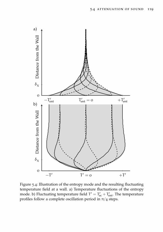
5.4 attenuation of sound 119
−T ′ent T ′ent = 0 +T ′ent
0
δχ
Dis
tanc
efr
omth
eW
all
−T ′ T ′ = 0 +T ′0
δχ
Dis
tanc
efr
omth
eW
all
a)
b)
Figure 5.4: Illustration of the entropy mode and the resulting fluctuatingtemperature field at a wall. a) Temperature fluctuations of the entropymode. b) Fluctuating temperature field T ′ = T ′ac + T
′ent. The temperature
profiles follow a complete oscillation period in π/4 steps.
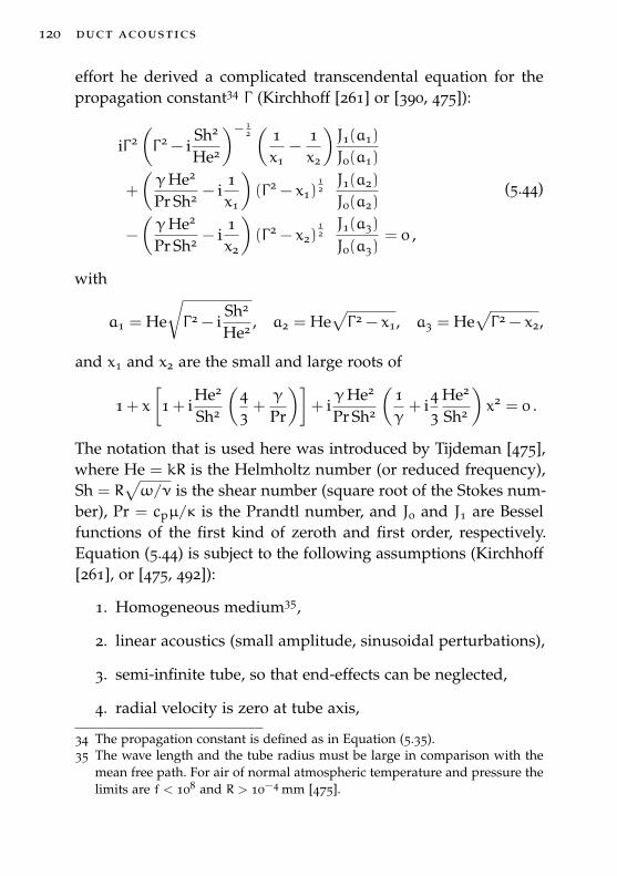
120 duct acoustics
effort he derived a complicated transcendental equation for thepropagation constant34 Γ (Kirchhoff [261] or [390, 475]):
iΓ 2(Γ 2 − i
Sh2
He2
)− 12(
1x1
−1x2
)J1(a1)
J0(a1)
+
(γHe2
Pr Sh2 − i1x1
)(Γ 2 − x1)
12J1(a2)
J0(a2)
−
(γHe2
Pr Sh2 − i1x2
)(Γ 2 − x2)
12J1(a3)
J0(a3)= 0 ,
(5.44)
with
a1 = He
√Γ 2 − i
Sh2
He2 , a2 = He√Γ 2 − x1, a3 = He
√Γ 2 − x2,
and x1 and x2 are the small and large roots of
1 + x
[1 + i
He2
Sh2
(43+γ
Pr
)]+ iγHe2
Pr Sh2
(1γ+ i
43
He2
Sh2
)x2 = 0 .
The notation that is used here was introduced by Tijdeman [475],where He = kR is the Helmholtz number (or reduced frequency),Sh = R
√ω/ν is the shear number (square root of the Stokes num-
ber), Pr = cpµ/κ is the Prandtl number, and J0 and J1 are Besselfunctions of the first kind of zeroth and first order, respectively.Equation (5.44) is subject to the following assumptions (Kirchhoff[261], or [475, 492]):
1. Homogeneous medium35,
2. linear acoustics (small amplitude, sinusoidal perturbations),
3. semi-infinite tube, so that end-effects can be neglected,
4. radial velocity is zero at tube axis,
34 The propagation constant is defined as in Equation (5.35).35 The wave length and the tube radius must be large in comparison with the
mean free path. For air of normal atmospheric temperature and pressure thelimits are f < 108 and R > 10−4 mm [475].
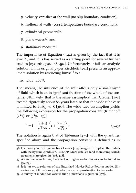
5.4 attenuation of sound 121
5. velocity vanishes at the wall (no-slip boundary condition),
6. isothermal walls (const. temperature boundary condition),
7. cylindrical geometry36,
8. plane waves37, and
9. stationary medium.
The importance of Equation (5.44) is given by the fact that it isexact38, and thus has served as a starting point for several furtherstudies [257, 261, 390, 448, 492]. Unfortunately, it fails an analyticsolution. In his original paper Kirchhoff [261] presents an approx-imate solution by restricting himself to a
10. wide tube39.
That means, the influence of the wall affects only a small layerof fluid which is an insignificant fraction of the whole of the con-tents. Ultimately, that is the same assumption that Cremer [101]treated rigorously about 80 years later, so that the wide tube caseis limited to δν,δχ � R [369]. The wide tube assumption yieldsthe following expression for the propagation constant (Kirchhoff[261], or [369, 475])
Γ = i +(1 + i)√
2 Sh
(1 +
γ− 1√Pr
). (5.45)
The notation is again that of Tijdeman [475] with the quantitiesspecified above and the propagation constant is defined as in
36 For non-cylindrical geometries Davies [113] suggest to replace the radiuswith the hydraulic radius rh = 2A/P. More detailed (and more complicated)treatments are given in [108, 448].
37 A discussion including the effect on higher order modes can be found in[36, 79].
38 It is an exact solution of the linearized Navier-Stokes-Fourier model (lin-earization of Equations 5.37), which are an approximation to first order.
39 A survey of models for various tube dimensions is given in [475].
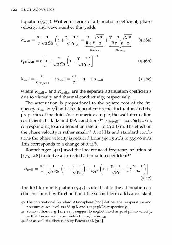
122 duct acoustics
Equation (5.35). Written in terms of attenuation coefficient, phasevelocity, and wave number this yields
αwall =ω
c
1√2 Sh
(1 +
γ− 1√Pr
)=
1R c
√νω
2︸ ︷︷ ︸αwall,ν
+γ− 1R c
√χω
2︸ ︷︷ ︸αwall,χ
(5.46a)
cph,wall = c
[1 +
1√2 Sh
(1 +
γ− 1√Pr
)]−1
(5.46b)
kwall =ω
cph,wall− iαwall =
ω
c+ (1 − i)αwall (5.46c)
where αwall,ν and αwall,χ are the separate attenuation coefficientsdue to viscosity and thermal conductivity, respectively.
The attenuation is proportional to the square root of the fre-quency αwall ∝
√f and also dependent on the duct radius and the
properties of the fluid. As a numeric example, the wall attenuationcoefficient at 1 kHz and ISA conditions40 is αwall = 0.0266 Np/m,corresponding to an attenuation rate a = 0.23 dB/m. The effect onthe phase velocity is rather small.41 At 1 kHz and standard condi-tions the phase velocity is reduced from 340.45 m/s to 339.96 m/s.This corresponds to a change of 0.14 %.
Ronneberger [411] used the low reduced frequency solution of[475, 508] to derive a corrected attenuation coefficient42
αwall =ω
c
[1√2 Sh
(1 +
γ− 1√Pr
)+
1Sh2
(1 +
γ− 1√Pr
−12γγ− 1
Pr
)].
(5.47)
The first term in Equation (5.47) is identical to the attenuation co-efficient found by Kirchhoff and the second term adds a constant
40 The International Standard Atmosphere [220] defines the temperature andpressure at sea level as 288.15 K and 101.325 kPa, respectively.
41 Some authors, e. g. [113, 115], suggest to neglect the change of phase velocity,so that the wave number yields k = ω/c− iαwall .
42 See as well the discussion by Peters et al. [366].
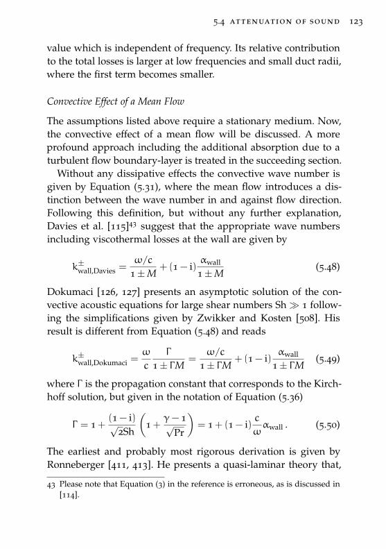
5.4 attenuation of sound 123
value which is independent of frequency. Its relative contributionto the total losses is larger at low frequencies and small duct radii,where the first term becomes smaller.
Convective Effect of a Mean Flow
The assumptions listed above require a stationary medium. Now,the convective effect of a mean flow will be discussed. A moreprofound approach including the additional absorption due to aturbulent flow boundary-layer is treated in the succeeding section.
Without any dissipative effects the convective wave number isgiven by Equation (5.31), where the mean flow introduces a dis-tinction between the wave number in and against flow direction.Following this definition, but without any further explanation,Davies et al. [115]43 suggest that the appropriate wave numbersincluding viscothermal losses at the wall are given by
k±wall,Davies =ω/c
1±M+ (1 − i)
αwall
1±M(5.48)
Dokumaci [126, 127] presents an asymptotic solution of the con-vective acoustic equations for large shear numbers Sh� 1 follow-ing the simplifications given by Zwikker and Kosten [508]. Hisresult is different from Equation (5.48) and reads
k±wall,Dokumaci =ω
c
Γ
1± ΓM=
ω/c
1± ΓM+ (1 − i)
αwall
1± ΓM(5.49)
where Γ is the propagation constant that corresponds to the Kirch-hoff solution, but given in the notation of Equation (5.36)
Γ = 1 +(1 − i)√
2Sh
(1 +
γ− 1√Pr
)= 1 + (1 − i)
c
ωαwall . (5.50)
The earliest and probably most rigorous derivation is given byRonneberger [411, 413]. He presents a quasi-laminar theory that,
43 Please note that Equation (3) in the reference is erroneous, as is discussed in[114].
124 duct acoustics
according to Peters et al. [366], describes the damping of acousticwaves quite accurately, when the acoustic boundary-layer thick-ness is small compared to the thickness of the viscous sublayer ofthe flow. To first order and with 1 − 0.18 M2 ≈ 1 (for small Machnumbers) Ronneberger results at [411]
k±wall,Ronneberger =ω/c
1±M+(1− i)
(αwall,ν
(1±M)3 +αwall,χ
(1±M)
), (5.51)
where αwall,ν and αwall,χ are the attenuation coefficients due to vis-cosity and thermal conductivity losses at the wall given in Equa-tion (5.46a), respectively.
The corresponding attenuation coefficients α±wall = −Im{k±}are plotted in Figure 5.5. While the attenuation is reduced in flowdirection, it increases against the flow, compared to the stationarycase αwall. The approach of Davies shows the smallest effect. Thevalues of Dokumaci’s and Ronneberger’s model are very close,but Ronneberger predicts a slightly stronger influence of the flow.The influence of convection on the phase velocity is visualizedin Figure 5.5b. Here, ∆c±ph,wall shows only the additional contri-bution that is introduced by the losses, so that for Davies andRonneberger the change is given by ∆c±ph,wall = c
±ph,wall − c (1±M)
and for Dokumaci ∆c±ph,wall = c±ph,wall − c (1±Re {Γ }M). While the
change of phase velocity in a stationary medium is small already,the convection introduces an even smaller variation around thatvalue. The results of Davies’ and Dokumaci’s models are identi-cal. They express a reduction of phase velocity in flow directionand an increase against the flow. Ronneberger’s model predictsthe opposite and a generally smaller effect.
Comparison to experimental data has shown [366] that Ron-neberger’s model includes the physical effects most accurately.However, browsing in recent literature it seems that Dokumaci’sapproach is the most accepted [13, 147, 205]. In the end, the smalldifferences in the result of these two models (Dokumaci vs. Ron-neberger) can be neglected in most practical applications.The limit that the acoustic boundary-layer thickness needs to be
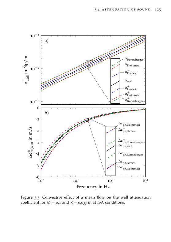
5.4 attenuation of sound 125
10−3
10−2
10−1
α−Ronneberger
α−Dokumaci
α−Davies
αwall
α+Davies
α+Dokumaci
α+Ronneberger
a)
α± w
all
inN
p/m
101 102 103 104-6
-5
-4
-3
-2
-1
0
∆c−ph,Dokumaci
∆c−ph,Davies
∆c+ph,Ronneberger∆cph,wall
∆c−ph,Ronneberger
∆c+ph,Davies
∆c+ph,Dokumaci
b)
Frequency in Hz
∆c± ph
, wal
lin
m/s
Figure 5.5: Convective effect of a mean flow on the wall attenuationcoefficient for M = 0.1 and R = 0.035 m at ISA conditions.
126 duct acoustics
smaller than the thickness of the viscous sublayer of the turbulentflow δν, δχ < δτ holds for all three models and is generally ful-filled for the parameters studied here, except for low frequenciesat high static pressures. When δν, δχ > δτ, then the additionallosses due to the interaction with the turbulent flow boundary-layer need to be considered. This is discussed in the next section.
5.4.2 Losses due to Turbulent Flow
The absorption of sound in a duct is increased by the presenceof a turbulent flow boundary-layer. This fact has been studiedexperimentally (e. g. [229, 366, 413]) and theoretically (e. g. [211,212, 229, 263, 366, 413, 490]). The additional absorption is due tothe transfer of acoustic energy to the turbulent stresses, a phe-nomenon which occurs when the acoustic boundary-layer thick-ness is larger than the viscous sublayer of the turbulent flow. Al-lam and Åbom [13] presented a comparison of the available mod-els and concluded that the model by Howe [212, 214] is the mostcomplete model developed so far44.Howe [212, 214] derives the following expression for the wavenumber, including the attenuation due to turbulent flow:
k±turb =ω/c
1±M+
2iρc(1±M)Dh
Y , (5.52)
where Y is the wall shear layer admittance
Y =e−
iπ4
ρω3/2
[(ω/c
1±M
)2√ν FA
(√iωνκ2v2∗
, δν
√iων
)
+βω2
cp
√χ FA
(Prt
√iωχκ2v2∗
, δν
√iωχ
)].
(5.53)
44 Since then, some extensions have been proposed in [263, 490], which are notincluded here.
5.4 attenuation of sound 127
Dh = 4A/P is the hydraulic diameter of the duct (with the ductcross-section area A and the duct perimeter P), κ is the Kármánconstant45 (please note that the same symbol was used to repre-sent thermal conductivity before), v∗ is the friction velocity, δν isthe thickness of the viscous acoustic boundary layer, β is the coef-ficient of expansion at constant pressure46, cp is the specific heatcapacity at constant pressure per unit of mass, Prt is the turbu-lence Prandtl number47, and
FA (a,b) =i[H
(1)1 (a) cos(b) −H(1)
0 (a) sin(b)]
H(1)0 (a) cos(b) +H(1)
1 (a) sin(b)(5.54)
with the Hankel functions48 H(1)m and H(2)
m . The friction velocity v∗can be computed from the empirical pipe flow formula [212, 432]
U(y)
v∗=
1κ
ln(v∗yν
)+C , (5.55)
where U(y) is the flow velocity at a specified distance from thewall y, κ is again the Kármán constant, and C is an empirical con-stant, usually specified as C = 5 [212, 432]. U(y) can be replacedby the mean flow velocity U, when setting y = R and C = 2 in theabove equation, where the adjustment of C accounts for the dif-ference between the mean flow velocity and the maximum flowvelocity at the centerline (y = R) of the duct [212, 432].The thickness of the viscous acoustic boundary layer δν is calcu-
lated from [212, 214]
δνv∗ν
= 6.5(
1 +σ(ω/ω∗)3
1 + (ω/ω∗)3
), (5.56)
45 Named after Theodore von Kármán (1881-1963, Hungarian-American math-ematician, aerospace engineer, and physicist) [256]. The Kármán constantis a universal constant for turbulent boundary layers. Its empirical value isκ = 0.41 [214, 432].
46 For an ideal gas β = 1/T , so that βc2/cp = γ− 1 [212]47 Schlichting and Gersten [432] state that Prt = 0.87, while Howe [212, 214]
gives a value of Prt = 0.7, which will be used here48 Named after Hermann Hankel (1839-1873, German mathematician). Also
known as Bessel functions of the third kind.
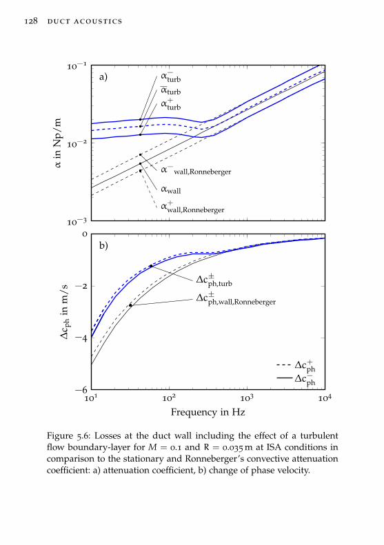
128 duct acoustics
α+wall,Ronneberger
αwall
α−wall,Ronneberger
α+turb
αturb
α−turba)
10−3
10−2
10−1α
inN
p/m
∆c±ph,wall,Ronneberger
∆c±ph,turb
b)
101 102 103 104−6
−4
−2
0
Frequency in Hz
∆c
phin
m/s
∆c+ph∆c−ph
Figure 5.6: Losses at the duct wall including the effect of a turbulentflow boundary-layer for M = 0.1 and R = 0.035 m at ISA conditions incomparison to the stationary and Ronneberger’s convective attenuationcoefficient: a) attenuation coefficient, b) change of phase velocity.
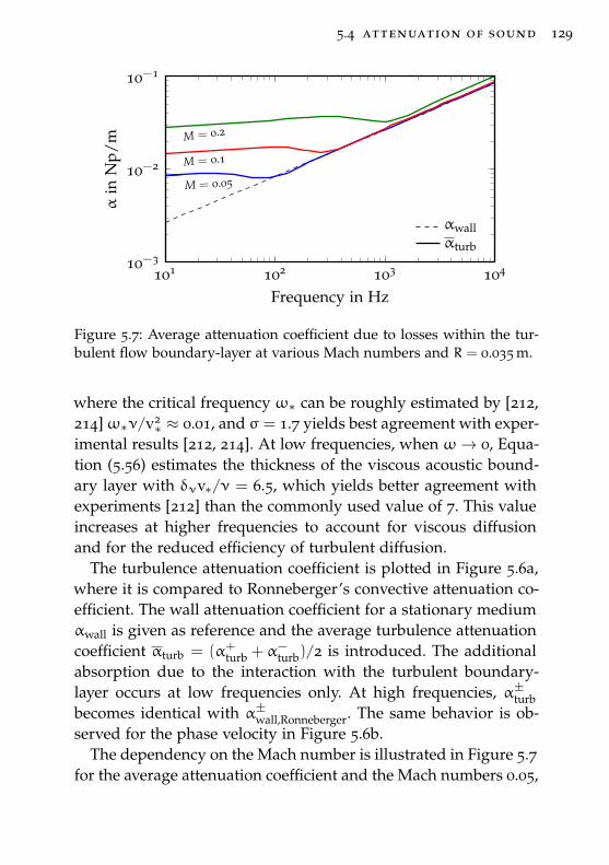
5.4 attenuation of sound 129
M = 0.05
M = 0.1
M = 0.2
101 102 103 10410−3
10−2
10−1
Frequency in Hz
αin
Np/
m
αwallαturb
Figure 5.7: Average attenuation coefficient due to losses within the tur-bulent flow boundary-layer at various Mach numbers and R = 0.035 m.
where the critical frequency ω∗ can be roughly estimated by [212,214]ω∗ν/v2
∗ ≈ 0.01, and σ = 1.7 yields best agreement with exper-imental results [212, 214]. At low frequencies, when ω→ 0, Equa-tion (5.56) estimates the thickness of the viscous acoustic bound-ary layer with δνv∗/ν = 6.5, which yields better agreement withexperiments [212] than the commonly used value of 7. This valueincreases at higher frequencies to account for viscous diffusionand for the reduced efficiency of turbulent diffusion.
The turbulence attenuation coefficient is plotted in Figure 5.6a,where it is compared to Ronneberger’s convective attenuation co-efficient. The wall attenuation coefficient for a stationary mediumαwall is given as reference and the average turbulence attenuationcoefficient αturb = (α+
turb + α−turb)/2 is introduced. The additional
absorption due to the interaction with the turbulent boundary-layer occurs at low frequencies only. At high frequencies, α±turbbecomes identical with α±wall,Ronneberger. The same behavior is ob-served for the phase velocity in Figure 5.6b.
The dependency on the Mach number is illustrated in Figure 5.7for the average attenuation coefficient and the Mach numbers 0.05,
130 duct acoustics
0.1, and 0.2. Generally, the losses due to the turbulent flow in-crease at higher Mach numbers, so that higher frequencies areaffected.
5.4.3 Losses Within the Fluid
At normal atmospheric temperature and pressure conditions, thelosses within the fluid become significant at high frequencies (be-yond the audible range) or when sound travels long distances.Such conditions are met when dealing with waves propagatingthrough the atmosphere, for example. In duct acoustics, these ef-fects are commonly neglected as they are two orders of magnitudesmaller than the losses at the duct walls. While this generallyholds for air at normal atmospheric temperature and pressure,it will be shown in Section 6.6.5 that the losses within the fluidmight become important at elevated pressure and temperature.
This section will be limited to a collection of the necessary for-mulas. A detailed historical review of the subject is presented byDelany [120] and an in-depth discussion of the physics is givenby Bass et al. [30]. Furthermore, the subject is treated extensivelyin the book of Pierce [369]. Today’s state of the art models thatdescribe the sound absorption within the fluid have been estab-lished in a series of publications by Evans et al. [152] and Basset al. [29, 31, 32], which ultimately led to the international stan-dard ISO 9613-1:1993 [236]. Bass [28] discussed the validity of theavailable models under high temperature conditions and came tothe conclusion that they are accurate within 10 % for low watervapor concentrations (less than 10 %).
The loss mechanisms within the fluid can be grouped into classi-cal absorption mechanisms, resulting from the fundamental trans-port properties of a fluid, and the losses based on the movementof the molecules, referred to as molecular relaxation losses.
5.4 attenuation of sound 131
Viscothermal Losses
The classical absorption is associated with the transfer of kineticenergy of molecules into heat. The responsible fluid properties areviscosity, thermal conductivity, diffusion, and radiation. However,the contribution of diffusion49 and radiation50 to the total lossesis very small, so that only the first two are considered here. There-fore, the classical absorption is also referred to as viscothermalabsorption.
The effect of viscosity on sound propagation has been treatedby Stokes [449, 451], and the dependency on thermal conductivityhas been introduced by Kirchhoff [261]. Both effects are additive,so that the classical attenuation coefficient due to viscothermalabsorption within the fluid is given as (Stokes [451] and Kirchhoff[261], or [30, 369])
αcl =ω2
2ρc343µ︸ ︷︷ ︸
viscosity
+ω2
2ρc3(γ− 1)κcp︸ ︷︷ ︸
thermal conductivity
=ω2µ
2ρc3
(43+γ− 1
Pr
). (5.57)
The classical attenuation coefficient is proportional to the squareof the frequency: αcl ∝ f2. It accurately describes the sound at-tenuation in a monoatomic gas. In polyatomic gases, for examplenitrogen and oxygen (the main constituents of air), the degrees offreedom within the molecules generate additional energy losses,so that the classical absorption underestimates the attenuation.
49 The effect of diffusion is known to be small, mainly because the two ma-jor constituents of air, nitrogen and oxygen, are of such similar molecularweights; as Rocard [404] and Herzfeld and Litovitz [196] have shown, thisprocess typically contributes only 0.3 % to the total classical absorption ataudio frequencies. (from [120])
50 The effect of radiation is very small (Stokes [450]). Radiation absorption playslittle role in gases, except possibly at very low pressures or very high tem-peratures (Markham et al. [314]). Radiation losses are significant only at verylow frequencies (Evans et al. [152]).
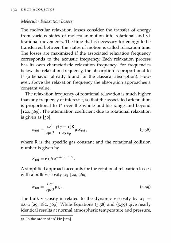
132 duct acoustics
Molecular Relaxation Losses
The molecular relaxation losses consider the transfer of energyfrom various states of molecular motion into rotational and vi-brational movements. The time that is necessary for energy to betransferred between the states of motion is called relaxation time.The losses are maximized if the associated relaxation frequencycorresponds to the acoustic frequency. Each relaxation processhas its own characteristic relaxation frequency. For frequenciesbelow the relaxation frequency, the absorption is proportional tof2 (a behavior already found for the classical absorption). How-ever, above the relaxation frequency the absorption approaches aconstant value.
The relaxation frequency of rotational relaxation is much higherthan any frequency of interest51, so that the associated attenuationis proportional to f2 over the whole audible range and beyond[120, 369]. The attenuation coefficient due to rotational relaxationis given as [30]
αrot =ω2
2ρc3γ(γ− 1)R
1.25 cpµZrot , (5.58)
where R is the specific gas constant and the rotational collisionnumber is given by
Zrot = 61.6 e−16.8T−1/3.
A simplified approach accounts for the rotational relaxation losseswith a bulk viscosity µB [29, 369]
αrot =ω2
2ρc3µB . (5.59)
The bulk viscosity is related to the dynamic viscosity by µB =
0.6µ [29, 182, 369]. While Equations (5.58) and (5.59) give nearlyidentical results at normal atmospheric temperature and pressure,
51 In the order of 108 Hz [120].
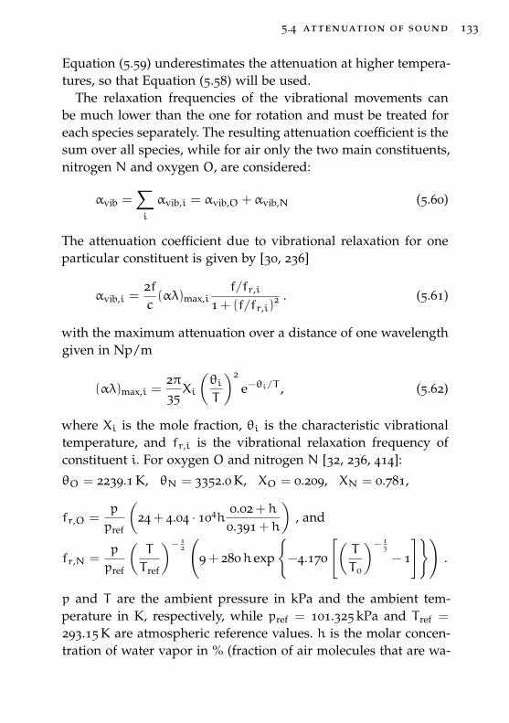
5.4 attenuation of sound 133
Equation (5.59) underestimates the attenuation at higher tempera-tures, so that Equation (5.58) will be used.
The relaxation frequencies of the vibrational movements canbe much lower than the one for rotation and must be treated foreach species separately. The resulting attenuation coefficient is thesum over all species, while for air only the two main constituents,nitrogen N and oxygen O, are considered:
αvib =∑i
αvib,i = αvib,O +αvib,N (5.60)
The attenuation coefficient due to vibrational relaxation for oneparticular constituent is given by [30, 236]
αvib,i =2fc(αλ)max,i
f/fr,i
1 + (f/fr,i)2 . (5.61)
with the maximum attenuation over a distance of one wavelengthgiven in Np/m
(αλ)max,i =2π35Xi
(θiT
)2
e−θi/T , (5.62)
where Xi is the mole fraction, θi is the characteristic vibrationaltemperature, and fr,i is the vibrational relaxation frequency ofconstituent i. For oxygen O and nitrogen N [32, 236, 414]:
θO = 2239.1 K, θN = 3352.0 K, XO = 0.209, XN = 0.781,
fr,O =p
pref
(24 + 4.04 · 104h
0.02 + h
0.391 + h
), and
fr,N =p
pref
(T
T ref
)− 12(
9 + 280h exp
{−4.170
[(T
T 0
)− 13
− 1
]}).
p and T are the ambient pressure in kPa and the ambient tem-perature in K, respectively, while pref = 101.325 kPa and T ref =
293.15 K are atmospheric reference values. h is the molar concen-tration of water vapor in % (fraction of air molecules that are wa-

134 duct acoustics
ter). It can be calculated from the relative humidity RH (also in %)via the saturation water vapor pressure pws [236, 369]
h = RHpws
p. (5.63)
While ISO 9613-1:1993 [236] presents a simplified calculation forpws, the state of the art formula is given by [485, 486]
ln(pws
pc
)=Tc
T
(a1ϑ+ a2ϑ
1.5 + a3ϑ3 + a4ϑ
3.5 + a5ϑ4 + a6ϑ
7.5)(5.64)
with
a1 = −7.85951783 a4 = −22.6807411 Tc = 647.096 K
a2 = −1.84408259 a5 = −15.9618719 pc = 22.064× 10⁶ Pa
a3 = −11.7866497 a6 = −1.80122502 ϑ = 1 − T/Tc
The saturation water vapor pressure is a function of temperatureand is defined for temperatures up to the critical point of water atTc, where the properties of the gas and liquid phase converge.
Combined Losses Within the Fluid
The losses within the fluid are additive52, so that they are givenby the sum
αfluid = αcl +αrot +αvib,O +αvib,N (5.65)
The classical and rotational relaxation losses are functions of pres-sure, temperature and frequency only. Often they are combinedin one expression αcr = αcl + αrot. The vibrational relaxation at-tenuation depends on the particular atmospheric constituent andthe mole fraction of water vapor, as well as pressure, temperature,and frequency.
52 Bass et al. [30] states that this is valid for frequencies up to 10 MHz.
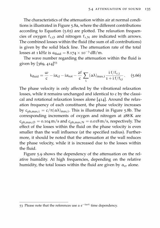
5.4 attenuation of sound 135
The characteristics of the attenuation within air at normal condi-tions is illustrated in Figure 5.8a, where the different contributionsaccording to Equation (5.65) are plotted. The relaxation frequen-cies of oxygen fr,O and nitrogen fr,N are indicated with arrows.The combined losses within the fluid (the sum of all contributions)is given by the solid black line. The attenuation rate of the totallosses at 1 kHz is afluid = 8.174× 10⁻³ dB/m.
The wave number regarding the attenuation within the fluid isgiven by [369, 414]53
kfluid =ω
c− iαcl − iαrot −
2fc
∑i
(αλ)max,ii f/fr,i
1 + i f/fr,i. (5.66)
The phase velocity is only affected by the vibrational relaxationlosses, while it remains unchanged and identical to c by the classi-cal and rotational relaxation losses alone [414]. Around the relax-ation frequency of each constituent, the phase velocity increasesby cph,max,i = c/π(αλ)max,i. This is illustrated in Figure 5.8b. Thecorresponding increments of oxygen and nitrogen at 288 K arecph,max,O = 0.104 m/s and cph,max,N = 0.018 m/s, respectively. Theeffect of the losses within the fluid on the phase velocity is evensmaller than the wall influence (at the specified radius). Further-more, it should be noted that the attenuation at the wall reducesthe phase velocity, while it is increased due to the losses withinthe fluid.
Figure 5.9 shows the dependency of the attenuation on the rel-ative humidity. At high frequencies, depending on the relativehumidity, the total losses within the fluid are given by αcr alone.
53 Please note that the references use a e−iωt time dependency.
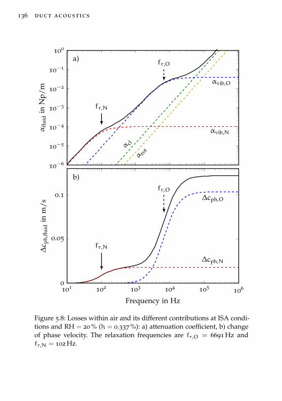
136 duct acoustics
α clα ro
t
αvib,O
αvib,N
fr,O
fr,N
a)
10−6
10−5
10−4
10−3
10−2
10−1
100α
fluid
inN
p/m
∆cph,O
∆cph,N
fr,O
fr,N
b)
101 102 103 104 105 1060
0.05
0.1
Frequency in Hz
∆c
ph,fl
uid
inm
/s
Figure 5.8: Losses within air and its different contributions at ISA condi-tions and RH = 20 % (h = 0.337 %): a) attenuation coefficient, b) changeof phase velocity. The relaxation frequencies are fr,O = 6691 Hz andfr,N = 102 Hz.
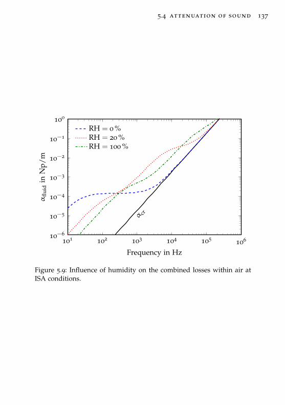
5.4 attenuation of sound 137
101 102 103 104 105 10610−6
10−5
10−4
10−3
10−2
10−1
100
α cr
Frequency in Hz
αflu
idin
Np/
m
RH = 0 %RH = 20 %RH = 100 %
Figure 5.9: Influence of humidity on the combined losses within air atISA conditions.

6E X P E R I M E N TA L M E T H O D & A N A LY S I S
The general methodology of the measurements is based on anapproach proposed by Ronneberger [411], which was developedfurther by Ronneberger and his students [74, 146, 360, 397–399,412]1. The same methodology, in principle, is commonly referredto as two-source scattering matrix method [1]. This method was usedfor liner or orifice characterization in [17, 83, 138, 198, 399], forexample.
For the evaluation of its acoustic performance, the lined ductsection is regarded as a black box and only the input and outputquantities are considered, i. e. the lined duct section is representedby an acoustical two-port2. The reflection and transmission coeffi-cients of a two-port can be determined from the incoming and out-going wave amplitudes based on two linearly independent mea-surements.
The liner is inserted in between two hard-walled duct sections,within which the acoustic pressure is measured at a minimum oftwo axial locations. Two acoustic measurements are performed,one with acoustic excitation from a loudspeaker located beyond
1 Unfortunately, most of these publications are hard-to-come-by reports, the-ses, or conference papers.
2 An acoustical two-port is a linear, physical system with one input and oneoutput port. The state at the input and output is fully defined by two statevariables, i. e. two independent physical quantities. Based on its origin fromelectrical network theory, sometimes the term four-pole is used instead oftwo-port. [1]
140 experimental method & analysis
the microphones in the first duct section and another one with asecond loudspeaker located beyond the microphones in the sec-ond duct section. Such a measurement pair is repeated for eachfrequency of interest.
6.1 spectral analysis
The time series data recorded by the microphones is transformedinto the frequency domain following the Welch method3 [488]. Inshort, that is the calculation of an averaged spectrum from over-lapped, windowed signal segments. Additionally, turbulent noiseis rejected by using a coherence function method as proposed byChung [95].
6.1.1 Welch Method
The Welch method is an extension and more generalized form ofthe Bartlett method [27] for spectral density estimation. The con-cept of the Bartlett method involves the averaging over several sig-nal segments in order to reduce the variance of the resulting spec-trum estimation. In order to reduce the leakage that is producedby calculating the Fourier transformation of non-periodic4 signals,Welch [488] proposes to apply a window function to each segment.However, using this procedure attenuates the signal at the begin-ning and end of each segment, so that more averages must betaken to obtain the same statistical accuracy of the estimated spec-trum, when compared to not using window functions. This wouldrequire a longer measurement time. Welch [488] overcomes thisby allowing the segments to overlap. The overlapping re-uses thedata attenuated by the window function and provides more seg-
3 Named after Peter D. Welch.4 For example, the non-periodicity of a harmonic sine signal is introduced by
taking time-series data of finite length, where the length does not correspondto multiples of the sine period.
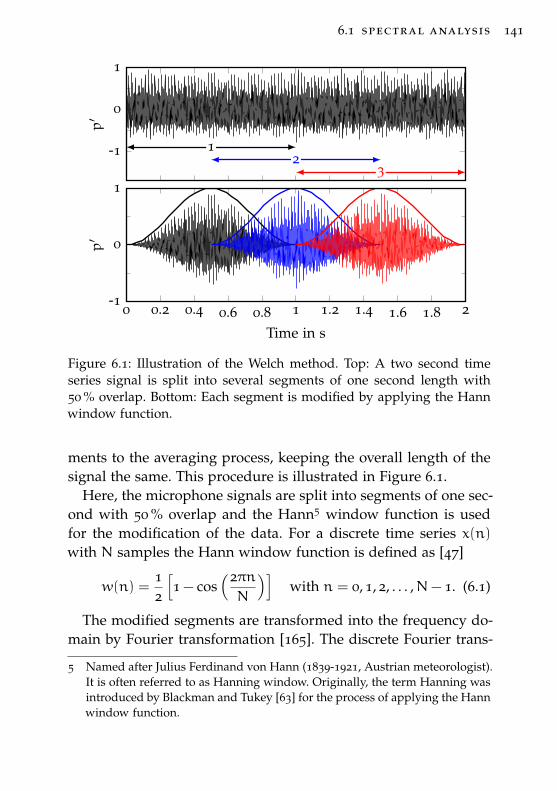
6.1 spectral analysis 141
12
3-1
0
1
p′
0 0.2 0.4 0.6 0.8 1 1.2 1.4 1.6 1.8 2-1
0
1
Time in s
p′
Figure 6.1: Illustration of the Welch method. Top: A two second timeseries signal is split into several segments of one second length with50 % overlap. Bottom: Each segment is modified by applying the Hannwindow function.
ments to the averaging process, keeping the overall length of thesignal the same. This procedure is illustrated in Figure 6.1.
Here, the microphone signals are split into segments of one sec-ond with 50 % overlap and the Hann5 window function is usedfor the modification of the data. For a discrete time series x(n)with N samples the Hann window function is defined as [47]
w(n) =12
[1 − cos
(2πnN
)]with n = 0, 1, 2, . . . ,N− 1. (6.1)
The modified segments are transformed into the frequency do-main by Fourier transformation [165]. The discrete Fourier trans-
5 Named after Julius Ferdinand von Hann (1839-1921, Austrian meteorologist).It is often referred to as Hanning window. Originally, the term Hanning wasintroduced by Blackman and Tukey [63] for the process of applying the Hannwindow function.
142 experimental method & analysis
formation X(k) of a discrete time signal x(n) with N samples isgiven by (e. g. [47])
X(k) =
N−1∑n=0
x(n) · e−i2πkn/N with k = 0, 1, 2, . . . ,N− 1. (6.2)
The use of a window function introduces some losses to the mag-nitude of the Fourier transformed signal. Using the Hann windowfunction X(k) can be corrected by multiplication with
√8/3.
The one-sided auto-spectral density, or short auto spectrum, isthen given by averaging over all segments s and normalizing withthe number of samples [47]
Gxx =
2SN
S∑s=1
|Xs(k)|2 for k = 1, 2, . . . , (N/2) − 1
1SN
S∑s=1
|Xs(k)|2 for k = 0, (N/2)
(6.3)
where S is the number of segments. Accordingly the one-sidedcross-spectral density, or short cross spectrum, of two signals x(n)and y(n) is given by [47]
Gxy =
2SN
S∑s=1
[X∗s(k) · Ys(k)] for k = 1, 2, . . . , (N/2) − 1
1SN
S∑s=1
[X∗s(k) · Ys(k)] for k = 0, (N/2)
(6.4)
where X∗ is the complex conjugate6 of X. In acoustics, the spec-trum is commonly scaled to the root-mean-square value by divi-sion with
√2.
6 The complex conjugate of the complex number z = a+ ib is given by invert-ing the sign of the imaginary part, i. e. z∗ = a− ib (e. g. [77]).
6.1 spectral analysis 143
6.1.2 Rejection of Flow Noise
The pressure fluctuations measured with the microphones are asuperposition of the sound pressure and flow induced turbulentpressure fluctuations. Chung [95] presents a method to reject theturbulent flow noise using three signals measured at different lo-cations. The basic premise is that the flow noise at these threepositions is uncorrelated, while the sound pressure is completelycoherent. The coherence between any two signals x and y is calcu-lated from the auto-spectral and cross-spectral densities [47]
γ2xy =
∣∣Gxy∣∣2 / (Gxx ·Gyy
). (6.5)
The ‘noise-free’ auto-spectral density G′xx yields [95]
G′11 = G11(γ12 · γ31
)/γ23 . (6.6)
The indexes 1, 2, and 3 refer to the three signals. Here, the signalof two microphones and the input signal of the loudspeaker areused. In that case index 1 refers to the target microphone, index 2to an arbitrary reference microphone, and index 3 to the speakerinput signal.
The result of Equation (6.6) is a real valued auto spectrum withunit Pa2. However, the plane wave decomposition (see Section 6.2below) relies on the phase information of each microphone. Thephase information is added by using the loudspeaker input signalas an arbitrary, but fixed for all microphones, phase reference. In-serting Equation (6.5) into (6.6) and adding the phase of the crosscorrelation between the target signal and the loudspeaker signalyields
G′11 =|G12| ·
∣∣G13∣∣∣∣G23
∣∣ ei arg(G13) . (6.7)
The complex pressure amplitude at the position of the target mi-crophone x1 is then given by p (x1, f) =
√G′11 (f).
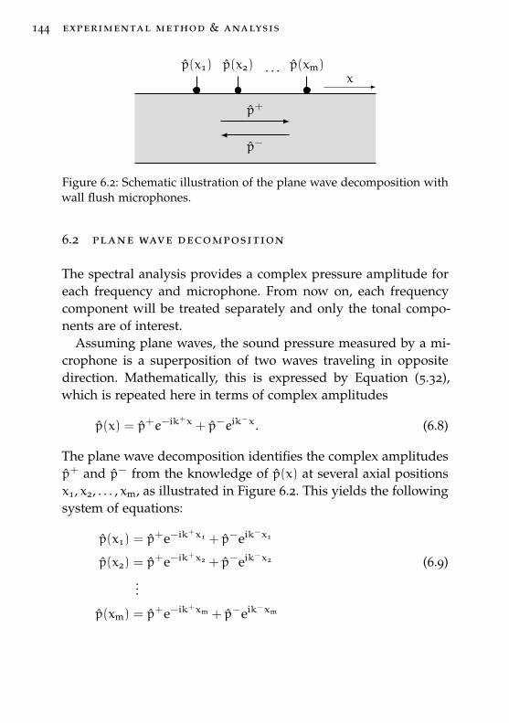
144 experimental method & analysis
draft – 2014.06.17 16:11 – claus lahiri
p+
p−
p(x1) p(x2) p(xm). . .x
Figure 6.2: Schematic illustration of the plane wave decomposition withwall flush microphones.
6.2 plane wave decomposition
The spectral analysis provides a complex pressure amplitude foreach frequency and microphone. From now on, each frequencycomponent will be treated separately and only the tonal compo-nents are of interest.
Assuming plane waves, the sound pressure measured by a mi-crophone is a superposition of two waves traveling in oppositedirection. Mathematically, this is expressed by Equation (5.32),which is repeated here in terms of complex amplitudes
p(x) = p+e−ik+x + p−eik−x. (6.8)
The plane wave decomposition identifies the complex amplitudesp+ and p− from the knowledge of p(x) at several axial positionsx1, x2, . . . , xm, as illustrated in Figure 6.2. This yields the followingsystem of equations:
p(x1) = p+e−ik+x1 + p−eik−x1
p(x2) = p+e−ik+x2 + p−eik−x2 (6.9)
...
p(xm) = p+e−ik+xm + p−eik−xm
6.2 plane wave decomposition 145
This system of linear equations can be written in matrix form ase−ikx1 eikx1
e−ikx2 eikx2
......
e−ikxm eikxm
︸ ︷︷ ︸
A
×[p+
p−
]︸ ︷︷ ︸
x
=
p(x1)
p(x2)...
p(xm)
︸ ︷︷ ︸
b
(6.10)
The size of the matrices is defined by the number of unknowns nand the number of available data m. Here, the unknowns are p+
and p−, so that n = 2, and m equals the number of microphonesat distinct axial positions. Then, the size of A is [m× 2], the size ofx is [2×1], and the size of b is [m×1]. A solution to Equation (6.10)can be obtained by solving [110]7
x = A+b (6.11)
where A+ is the Moore-Penrose pseudoinverse8 of matrix A. Whilean inverse matrix only exists for square matrices, the pseudoin-verse is a unique, generalized inverse that exists for matrices ofany size. It can be calculated from the singular value decompo-sition9 of matrix A. The singular value decomposition is the fac-torization of the matrix A into the product of a unitary10 matrix
7 The reference gives an overview of other solution methods as well.8 The Moore-Penrose pseudoinverse is named after Eliakim Hastings Moore
(1862-1932, American mathematician), [334], and Sir Roger Penrose (born1931, English mathematical physicist), [365]. Sometimes it is called general-ized inverse or just pseudoinverse. More details can be found in [110] or[179], for example.
9 The singular value decomposition originates from the works of E. Beltrami(1835-1899, Italian mathematician) [45], C. Jordan (1838-1921, French mathe-matician) [249, 250], J.J. Sylvester (1814-1897, English mathematician) [464–466], E. Schmidt (1876-1959, German mathematician) [433], and H. Weyl(1885-1955, German mathematician and theoretical physicist) [493]. Stewart[446] gives an historical overview from where the original references aretaken. More details can be found in [110] or [179], for example.
10 A unitary matrix U is a complex-valued, square matrix, for which UhU =
I, where I is the identity matrix. The real-valued equivalent to the unitarymatrix is the orthogonal matrix. [110]
146 experimental method & analysis
U, a diagonal matrix Σ, and another unitary matrix Vh, so thatA = UΣVh, where Vh is the Hermitian transpose11 of V [110].Then, the pseudoinverse is given by A+ = VΣ+Uh [110]. This so-lution method is very universal, as it can be used with matricesof any size and even badly conditioned matrices, e.g. singular ornear-singular matrices, can be handled.
A solution to Equation (6.10) exists, if at least two equationsare linearly independent. This means, microphones need to beinstalled at least at two distinct axial positions. Generally, it canbe distinguished between two cases, depending on the number ofmicrophones:
1. The number of equations/microphones and the number ofunknowns are equal. This is commonly referred to as thetwo-microphone method.
2. The number of equations/microphones is greater than thenumber of unknowns. This is commonly referred to as themulti-microphone method.
The two-microphone method is established as a standardized mea-surement method defined in ISO 10534-2:1998 [232] and ASTM E1050-12 [22]. It was initially proposed, in slightly varying forms,by Johnston & Schmidt [245], Seybert & Ros [437], and Chung& Blaser [96]. With only two linearly independent equations, thesystem in Equation (6.10) has one unique solution. The sensitivityto errors has been studied by several authors, in particular [2, 69,218, 435, 438]. One restriction of the two-microphone method is,that the solution becomes singular when ks = nπ, where s is thespacing between the microphones and n = {0, 1, 2, . . . }. For n = 1this corresponds to a spacing of half a wave length
s = λ/2 . (6.12)
11 The Hermitian transpose, or sometimes called conjugate transpose, is de-fined as V
h = (V∗)t, where Vt denotes the transpose and V
∗ denotes thematrix with complex conjugated entries. [110]
6.2 plane wave decomposition 147
The errors increase rapidly in the vicinity of these singularities,so that Åbom and Bodén [2] suggest to limit the two-microphonemethod to the frequency range
0.1π <ks
1 − M2 < 0.8π , (6.13)
which includes the influence of mean flow in the duct.
The multi-microphone method yields an overdetermined sys-tem of equations. The solution given by Equation (6.11) is a bestfit in the least-squares12 sense. Experimental methods that makeuse of a least-squares fitting procedure over 3+ microphone posi-tions are presented in [167, 246, 411, 412]. Generally, the accuracyof the results can be improved by using more than two micro-phones [94, 237, 246]. The effect of the number and spacing of themicrophones was studied by Jones [246] and Jang and Ih [237].Both conclude that an equidistant microphone spacing deliversthe best results. However, the problem with a singular solution ata certain microphone spacing remains. The influence of the singu-lar solution is reduced to a smaller frequency range when usingmore microphones.
Brandes [74] investigates the influence of different microphonedistributions on the error in the scattering coefficients. He requiresaccurate measurements over a large frequency range (20-4000 Hz).An exponential distribution, where the spacing increases with afactor of 1.72, fulfills this requirement best. He demonstrates, thatthe density of the microphones should be higher towards the testobject. This reduces errors when extrapolating the result of thewave decomposition from the microphone section to the test ob-ject. This approach has been followed at the DUCT-C and HATfacilities (see Section 6.5 and 6.6, respectively). The microphonesare distributed exponentially with a factor of 1.62 (DUCT-C) and1.72 (HAT).
12 The method of least-squares minimizes the sum of squared residuals [60].This principle was introduced by Legendre [293] and Gauss [172].
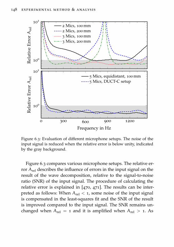
148 experimental method & analysis
100
101
Rel
ativ
eEr
rorA
rel 2 Mics, 100 mm
2 Mics, 200 mm3 Mics, 100 mm3 Mics, 200 mm
0 300 600 900 1200
100
101
Frequency in Hz
Rel
ativ
eEr
rorA
rel 5 Mics, equidistant, 100 mm
5 Mics, DUCT-C setup
Figure 6.3: Evaluation of different microphone setups. The noise of theinput signal is reduced when the relative error is below unity, indicatedby the gray background.
Figure 6.3 compares various microphone setups. The relative er-ror Arel describes the influence of errors in the input signal on theresult of the wave decomposition, relative to the signal-to-noiseratio (SNR) of the input signal. The procedure of calculating therelative error is explained in [470, 471]. The results can be inter-preted as follows: When Arel < 1, some noise of the input signalis compensated in the least-squares fit and the SNR of the resultis improved compared to the input signal. The SNR remains un-changed when Arel = 1 and it is amplified when Arel > 1. As
6.2 plane wave decomposition 149
a consequence, a good microphone distribution should achieveArel 6 1 for the relevant frequency range.
The top plot in Figure 6.3 compares microphone setups withtwo and three microphones, spaced equidistantly by 100 mm and200 mm. At the long distance, condition (6.12) is fulfilled at 850 Hz,resulting in large errors when using either two or three micro-phones. This singularity moves to 1700 Hz, just outside the fre-quency range, when using the tighter spacing. At the same timethe error at low frequencies is increasing. The phase differencebetween two microphones becomes smaller at low frequencies, orrather when the wave length is long. The amount of noise and thedistance between the microphones determines the frequency un-til which the wave decomposition is able to resolve a small phasedifference. Using two microphones, yields only a very limited fre-quency range where Arel is just below unity. Adding a third mi-crophone generally improves the result dramatically. Three micro-phones should really be the minimum configuration, especiallyfor measurements with flow. The low frequency error is mainlydependent on the maximum distance between two microphones.Thus, the results at f < 400 Hz is nearly identical for two micro-phones spaced at 200 mm or three microphones at 100 mm each.
The plot at the bottom of Figure 6.3 compares a five micro-phone equidistant distribution to the exponential distribution ofthe DUCT-C. Both results are very similar. At low frequenciesthe DUCT-C setup is slightly better than the equidistant setupdue to its longer maximum distance between the microphones,i. e. 531 mm compared to 400 mm, respectively. What is not visiblehere, is that the error of the equidistant setup will of course peakat 1700 Hz, while the DUCT-C setup will not. However, for thefrequency range here the dissipation coefficient measured witheither microphone distributions would probably be identical.
A typical result of a plane wave decomposition from DUCT-Cdata is presented in Figure 6.4. p is measured at five axial po-sitions xm in a hard-walled duct section. The solution to Equa-
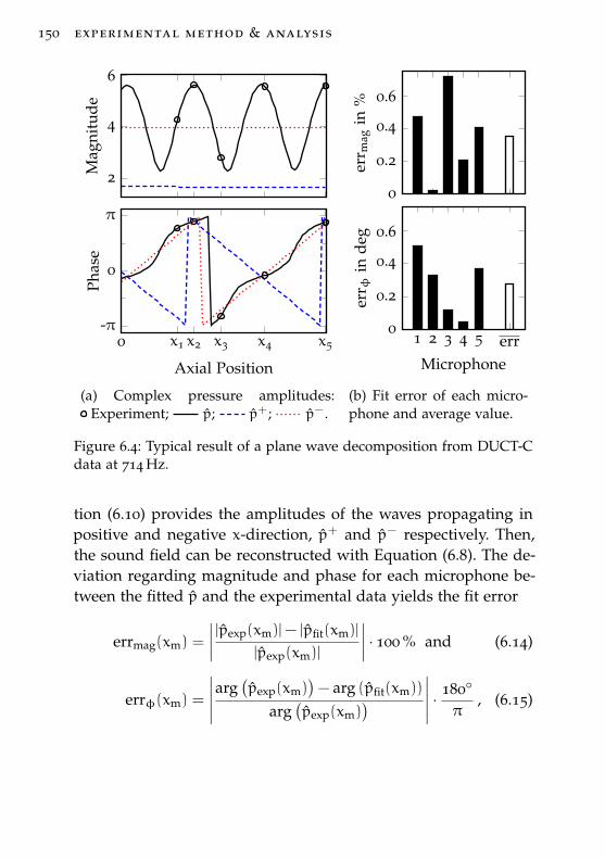
150 experimental method & analysis
2
4
6M
agni
tude
0 x1 x2 x3 x4 x5
-π
0
π
Axial Position
Phas
e
(a) Complex pressure amplitudes:Experiment; p; p+; p−.
0
0.2
0.4
0.6
err m
agin
%1 2 3 4 5 err
0
0.2
0.4
0.6
Microphoneer
r φin
deg
(b) Fit error of each micro-phone and average value.
Figure 6.4: Typical result of a plane wave decomposition from DUCT-Cdata at 714 Hz.
tion (6.10) provides the amplitudes of the waves propagating inpositive and negative x-direction, p+ and p− respectively. Then,the sound field can be reconstructed with Equation (6.8). The de-viation regarding magnitude and phase for each microphone be-tween the fitted p and the experimental data yields the fit error
errmag(xm) =
∣∣∣∣ |pexp(xm)|− |pfit(xm)|
|pexp(xm)|
∣∣∣∣ · 100 % and (6.14)
errφ(xm) =
∣∣∣∣∣arg(pexp(xm)
)− arg (pfit(xm))
arg(pexp(xm)
) ∣∣∣∣∣ · 180◦
π, (6.15)
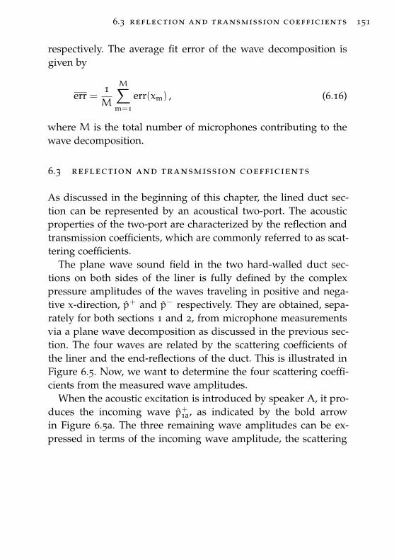
6.3 reflection and transmission coefficients 151
respectively. The average fit error of the wave decomposition isgiven by
err =1M
M∑m=1
err(xm) , (6.16)
where M is the total number of microphones contributing to thewave decomposition.
6.3 reflection and transmission coefficients
As discussed in the beginning of this chapter, the lined duct sec-tion can be represented by an acoustical two-port. The acousticproperties of the two-port are characterized by the reflection andtransmission coefficients, which are commonly referred to as scat-tering coefficients.
The plane wave sound field in the two hard-walled duct sec-tions on both sides of the liner is fully defined by the complexpressure amplitudes of the waves traveling in positive and nega-tive x-direction, p+ and p− respectively. They are obtained, sepa-rately for both sections 1 and 2, from microphone measurementsvia a plane wave decomposition as discussed in the previous sec-tion. The four waves are related by the scattering coefficients ofthe liner and the end-reflections of the duct. This is illustrated inFigure 6.5. Now, we want to determine the four scattering coeffi-cients from the measured wave amplitudes.
When the acoustic excitation is introduced by speaker A, it pro-duces the incoming wave p+1a, as indicated by the bold arrowin Figure 6.5a. The three remaining wave amplitudes can be ex-pressed in terms of the incoming wave amplitude, the scattering
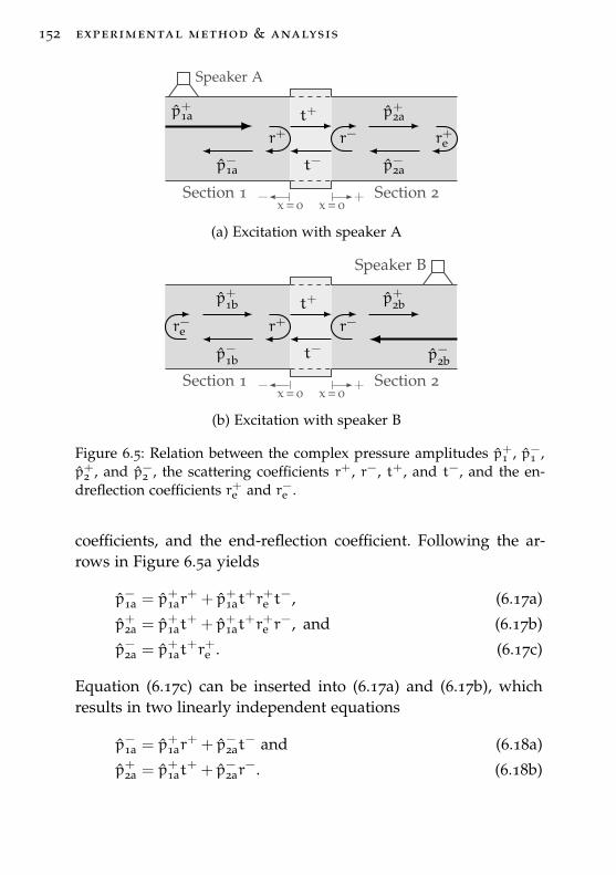
152 experimental method & analysis
Section 1 Section 2
Speaker A
p+1a
p−1a
p+2a
p−2a
r+ r−t+
t−
r+e
x= 0+
x= 0−
(a) Excitation with speaker A
Section 1 Section 2
Speaker B
p+1b
p−1b
p+2b
p−2b
r+ r−t+
t−
r−e
x= 0+
x= 0−
(b) Excitation with speaker B
Figure 6.5: Relation between the complex pressure amplitudes p+1 , p−1 ,p+2 , and p−2 , the scattering coefficients r+, r−, t+, and t−, and the en-dreflection coefficients r+e and r−e .
coefficients, and the end-reflection coefficient. Following the ar-rows in Figure 6.5a yields
p−1a = p+1ar+ + p+1at
+r+e t−, (6.17a)
p+2a = p+1at+ + p+1at
+r+e r−, and (6.17b)
p−2a = p+1at+r+e . (6.17c)
Equation (6.17c) can be inserted into (6.17a) and (6.17b), whichresults in two linearly independent equations
p−1a = p+1ar+ + p−2at
− and (6.18a)
p+2a = p+1at+ + p−2ar
−. (6.18b)
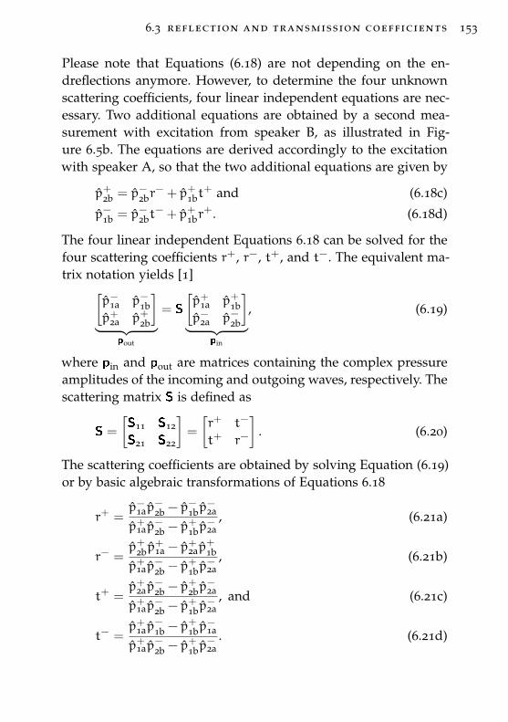
6.3 reflection and transmission coefficients 153
Please note that Equations (6.18) are not depending on the en-dreflections anymore. However, to determine the four unknownscattering coefficients, four linear independent equations are nec-essary. Two additional equations are obtained by a second mea-surement with excitation from speaker B, as illustrated in Fig-ure 6.5b. The equations are derived accordingly to the excitationwith speaker A, so that the two additional equations are given by
p+2b = p−2br− + p+1bt
+ and (6.18c)
p−1b = p−2bt− + p+1br
+. (6.18d)
The four linear independent Equations 6.18 can be solved for thefour scattering coefficients r+, r−, t+, and t−. The equivalent ma-trix notation yields [1][
p−1a p−1bp+2a p+2b
]︸ ︷︷ ︸
pout
= S
[p+1a p+1bp−2a p−2b
]︸ ︷︷ ︸
pin
, (6.19)
where pin and pout are matrices containing the complex pressureamplitudes of the incoming and outgoing waves, respectively. Thescattering matrix S is defined as
S =
[S11 S12
S21 S22
]=
[r+ t−
t+ r−
]. (6.20)
The scattering coefficients are obtained by solving Equation (6.19)or by basic algebraic transformations of Equations 6.18
r+ =p−1ap
−2b − p
−1bp
−2a
p+1ap−2b − p
+1bp
−2a
, (6.21a)
r− =p+2bp
+1a − p
+2ap
+1b
p+1ap−2b − p
+1bp
−2a
, (6.21b)
t+ =p+2ap
−2b − p
+2bp
−2a
p+1ap−2b − p
+1bp
−2a
, and (6.21c)
t− =p+1ap
−1b − p
+1bp
−1a
p+1ap−2b − p
+1bp
−2a
. (6.21d)
154 experimental method & analysis
With above equations, the reflection and transmission coefficientsof the liner can be calculated directly from the incoming and out-going wave amplitude of two independent measurements. Theindependence of the measurements is achieved by applying theso-called two-source location method [1, 344], where the sound issubsequently incident from either side of the liner.
An alternative approach is the two-load method [307, 344, 476,477], commonly with the source fixed at one end of the duct andvarying the load, e. g. the length, at the opposite end. While thismethod is generally inferior to the two-source location method[344], it could be the only option when the source cannot bemoved, e. g. in a combustion test rig with acoustic excitation bythe flame.
A variation of the two-source location method is proposed byEnghardt [146], where both speakers are operated simultaneously.Two independent sound fields are produced by keeping the phaseof the input signal constant for one speaker, while the phase ofthe second speaker is shifted by 180° between the measurements.The simultaneous excitation on both sides ensures good signal-to-noise ratios in both duct sections, even when the transmissioncoefficient of the test object is near zero.
6.4 dissipation coefficient
An acoustical two-port is characterized by its reflection and trans-mission coefficients, as defined above. A derived quantity is theenergy dissipation coefficient D, which is used here to evaluatethe acoustic performance of the liner. In energy terms, the sum ofreflection, transmission, and dissipation coefficient is unity
R± + T± +D± = 1 . (6.22)
R and T are the energy reflection and transmission coefficients,respectively, while r and t have been the pressure reflection andtransmission coefficients. The energy and pressure quantities are
6.4 dissipation coefficient 155
related by the acoustic energy flux P. For plane waves in a ductwith cross-section area A and mean flow Mach number M theenergy flux yields [66]13
P± =A
2ρc(1±M)2 ∣∣p±∣∣2 . (6.23)
This expression relates the acoustic pressure p to the acoustic en-ergy flux P. Accordingly, it can be applied to calculate R and T
from r and t, respectively. Combining Equations (6.22) and (6.23),the energy dissipation coefficient is defined as
D± = 1−((1∓M1)
2
(1±M1)2 ·∣∣r±∣∣2 + ρ1c1
ρ2c2
A2
A1
(1±M2)2
(1±M1)2 ·∣∣t±∣∣2) , (6.24)
where the indexes 1 and 2 refer to the quantities in section 1 andsection 2 as defined in Figure 6.5. When the duct cross-section areaand the thermodynamic conditions are the same in both sections,Equation (6.24) reduces to14
D± = 1 −
((1∓M1)
2
(1±M1)2 ·∣∣r±∣∣2 + (1±M2)
2
(1±M1)2 ·∣∣t±∣∣2) . (6.25)
6.4.1 Average Dissipation Coefficient
Averaging the dissipation coefficients in positive and negative x-direction yields the average dissipation
D =(D+ +D−
)/2 . (6.26)
The + and − dissipation coefficents are equal when the liner con-figuration is symmetric and Mg = 0. In that case D+ = D− = D
13 See as well the derivations in [374, 412] or the entry in Morfey’s dictonary[338] under ‘Blokhintsev invariant’.
14 A bias flow liner injects mass flow into the duct in-between the two sections,so that always M1 6= M2. However, if mb � mg or M ≈ 0 (when includingthe additional mass flow), then the difference can be neglected and Equa-tion (6.25) can be reduced further.
156 experimental method & analysis
and using D is merely a reduction of data. An asymmetric con-figuration or a grazing flow yields D+ 6= D−. The grazing flowreduces the dissipation in flow direction while increasing it forwaves propagating against the flow. Then, a comparison of D al-lows the evaluation of the overall performance of the liner, takingboth directions into account.For example in a combustor, where the main source of sound isthe flame, the sound wave travels in flow direction away from theflame and is then reflected at the combuster exit traveling againstflow direction towards the flame. In order to suppress the acousticfeedback to the flame D+ and D− are equally important, so thatthe overall performance can be evaluated by their mean value D.
6.4.2 Dissipation Error
The error that is made when measuring the dissipation coefficientcan be determined by a reference measurement without liner. Themeasurement and analysis procedure is the same as if a liner waspresent. However, without liner the theoretical result is knownand yields R± = 0, T± = 1, and D± = 0. The dissipation error isdefined as the absolute deviation from this expected value, aver-aged over both directions and expressed in percent
Derr =
∣∣D+ref
∣∣+ ∣∣D−ref
∣∣2
· 100 %. (6.27)
The dissipation error is a measure of the accuracy of the results. Itis in particular useful when evaluating different setups or changesin the data analysis (see Sections 6.5.2 and 6.5.4).
6.4.3 Compared to the Absorption Coefficient
Eldredge and Dowling [142] use the absorption coefficient to eval-uate the performance of the liner, see Equation (4.78). The absorp-tion and dissipation coefficients follow the same principle, rep-resenting the difference between incoming and outgoing energy.
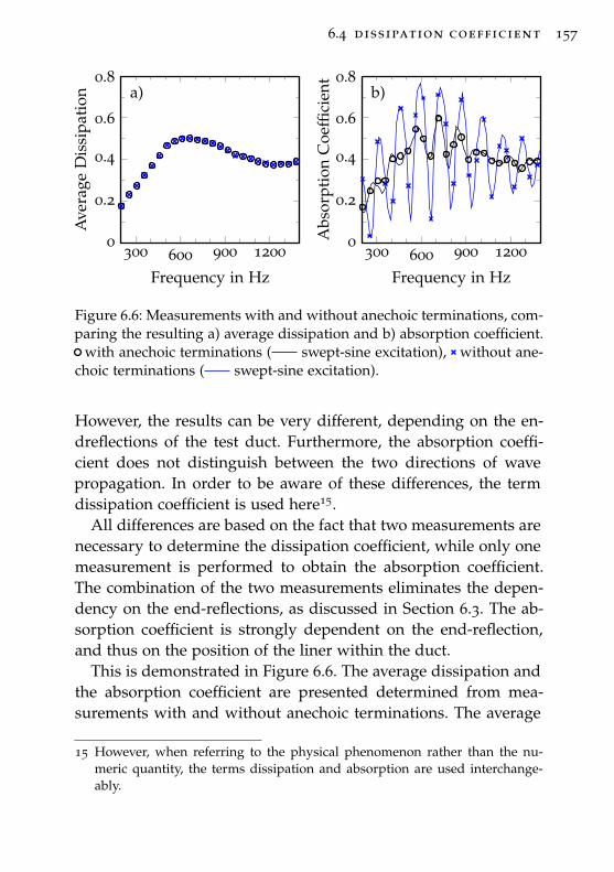
6.4 dissipation coefficient 157
300 600 900 12000
0.2
0.4
0.6
0.8a)
Frequency in Hz
Ave
rage
Dis
sipa
tion
300 600 900 12000
0.2
0.4
0.6
0.8b)
Frequency in Hz
Abs
orpt
ion
Coe
ffici
ent
Figure 6.6: Measurements with and without anechoic terminations, com-paring the resulting a) average dissipation and b) absorption coefficient.
with anechoic terminations ( swept-sine excitation), without ane-choic terminations ( swept-sine excitation).
However, the results can be very different, depending on the en-dreflections of the test duct. Furthermore, the absorption coeffi-cient does not distinguish between the two directions of wavepropagation. In order to be aware of these differences, the termdissipation coefficient is used here15.
All differences are based on the fact that two measurements arenecessary to determine the dissipation coefficient, while only onemeasurement is performed to obtain the absorption coefficient.The combination of the two measurements eliminates the depen-dency on the end-reflections, as discussed in Section 6.3. The ab-sorption coefficient is strongly dependent on the end-reflection,and thus on the position of the liner within the duct.
This is demonstrated in Figure 6.6. The average dissipation andthe absorption coefficient are presented determined from mea-surements with and without anechoic terminations. The average
15 However, when referring to the physical phenomenon rather than the nu-meric quantity, the terms dissipation and absorption are used interchange-ably.
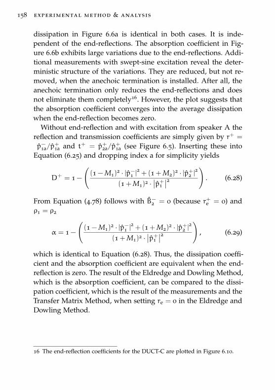
158 experimental method & analysis
dissipation in Figure 6.6a is identical in both cases. It is inde-pendent of the end-reflections. The absorption coefficient in Fig-ure 6.6b exhibits large variations due to the end-reflections. Addi-tional measurements with swept-sine excitation reveal the deter-ministic structure of the variations. They are reduced, but not re-moved, when the anechoic termination is installed. After all, theanechoic termination only reduces the end-reflections and doesnot eliminate them completely16. However, the plot suggests thatthe absorption coefficient converges into the average dissipationwhen the end-reflection becomes zero.
Without end-reflection and with excitation from speaker A thereflection and transmission coefficients are simply given by r+ =
p−1a/p+1a and t+ = p+2a/p
+1a (see Figure 6.5). Inserting these into
Equation (6.25) and dropping index a for simplicity yields
D+ = 1 −
((1 − M1)
2 · |p−1 |2+ (1 + M2)
2 · |p+2 |2
(1 + M1)2 ·∣∣p+1 ∣∣2
). (6.28)
From Equation (4.78) follows with B−2 = 0 (because r+e = 0) and
ρ1 = ρ2
α = 1 −
((1 − M1)
2 · |p−1 |2+ (1 + M2)
2 · |p+2 |2
(1 + M1)2 ·∣∣p+1 ∣∣2
), (6.29)
which is identical to Equation (6.28). Thus, the dissipation coeffi-cient and the absorption coefficient are equivalent when the end-reflection is zero. The result of the Eldredge and Dowling Method,which is the absorption coefficient, can be compared to the dissi-pation coefficient, which is the result of the measurements and theTransfer Matrix Method, when setting re = 0 in the Eldredge andDowling Method.
16 The end-reflection coefficients for the DUCT-C are plotted in Figure 6.10.
6.5 duct acoustic test rig 159
6.5 duct acoustic test rig
The Duct Acoustic Test Rig (DUCT) provides three setups with dif-ferent cross-section geometries of the measurement sections. Here,the circular cross-section (DUCT-C) is used.
6.5.1 Setup & Instrumentation
A schematic setup of the DUCT-C is shown in Figure 6.7. Thetest rig consists of two symmetric measurement sections with theliner module in-between and anechoic terminations17 at both ends.Each section is made of an 1200 mm long aluminum tube with aninner diameter of 140 mm. Two loudspeakers are installed at thecircumference of the duct at x = ±1041 mm. They are connectedto the duct via a conical horn. In order to reduce the interactionbetween the grazing flow and the opening it is covered by a per-forate within the duct. A total of 12 microphones are mountedflush with the duct wall. The microphones are distributed overten axial positions with a higher density towards the liner. Twomicrophones are installed at the two outermost positions closeto the loudspeakers. The two microphones are mounted oppositeeach other, canceling out evanescent modes generated by the loud-speaker18. The maximum axial distance between the microphonesin each section is 531 mm and the minimum distance between thetwo innermost microphones is 60 mm.
Two liner modules of different lengths are available, so that lin-ers with a length of 60 mm and 280 mm can be studied. The di-ameter of the liners is identical to the duct diameter. The innerdiameter of the cavity of both modules is 240 mm. A second linercan be inserted concentric to the first one at diameters 162, 192,212 mm in the shorter version and only at 162 mm in the longerversion. There are four inlets for the bias flow at the outer cir-
17 The effectiveness of the anechoic termination is demonstrated in Figure 6.10.18 The influence of evanescent modes is discussed in Section 6.5.4.
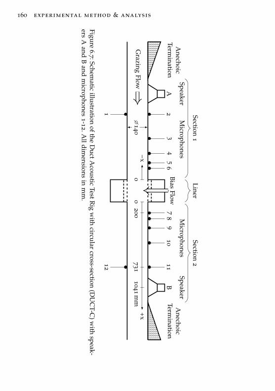
160 experimental method & analysis
dr
aft
–2014.06.17
16:13–
cla
us
lah
iri
Anechoic
Termination
Liner
A
Speaker
65
43
21
Microphonesp
Section1
Anechoic
Termination
B
Speaker
78
910
1112
Microphonesp
Section2
Grazing
Flow
BiasFlow
+−x
0+x
0200
mm
1041m
m731
�140
Figur e6.7:Schem
aticillustration
oftheD
uctAcoustic
TestRig
with
circularcross-section
(DU
CT-C
)with
speak-ers
Aand
Band
microphones
1-12.Alldim
ensionsin
mm
.
6.5 duct acoustic test rig 161
cumference, distributed with an even pitch of 90◦. In the shortmodule they are centered axially and discharge into the cavity inradial direction through an opening of diameter 17.8 mm. In thelonger version, the inlets are at the upstream end of the cavitywith tubes extending into the cavity and directing the bias flow inaxial direction.
The bias flow is controlled with a Bronkhorst ELFlow mass flowcontroller with a maximum flow rate of 100 kg/h. At the sametime, the pressure difference across the liner is measured with aMKS Baratron differential pressure meter. In the rare case whenhigher mass flow rates are needed, the controller is excluded andthe flow rate is set manually by adjusting the line pressure. How-ever, no mass flow information is available in this approach.
The maximum mean grazing flow Mach number is 0.13. Thegrazing flow Reynolds number of all velocities studied here islarger than the critical Reynolds number Rec = 4000 (e. g. [495]),so that the flow can be considered fully turbulent. This was con-firmed by velocity profile measurements [197].
The temperature of the flow is measured in section 2 of the testduct with a J-type thermocouple connected directly to an Agilent34970A data acquisition / data logger switch unit.
The acoustic test signal is a multi-tone sine signal. Three signalshave been synthesized containing eight tones each:
signal 1 : 204, 255, 306, 357, 459, 561, 663, 867 Hz
signal 2 : 408, 510, 612, 714, 765, 969, 1071, 1173 Hz
signal 3 : 816, 918, 1020, 1122, 1224, 1275, 1326, 1377 Hz
The frequencies are distributed between the signals, so that nomultiples of a frequency are contained in one signal. All threesignals together cover a frequency range from 204 to 1377 Hz insteps of 51 Hz. All tonal components are in the plane wave range,i. e. their frequencies are below19 1413 Hz. The signal has been
19 Defined by Equation (5.19) for speed of sound at ISA conditions and themaximum grazing flow Mach number.
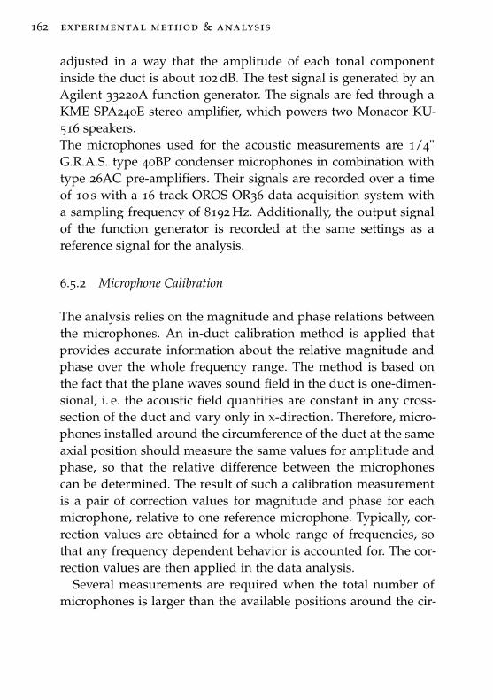
162 experimental method & analysis
adjusted in a way that the amplitude of each tonal componentinside the duct is about 102 dB. The test signal is generated by anAgilent 33220A function generator. The signals are fed through aKME SPA240E stereo amplifier, which powers two Monacor KU-516 speakers.The microphones used for the acoustic measurements are 1/4"G.R.A.S. type 40BP condenser microphones in combination withtype 26AC pre-amplifiers. Their signals are recorded over a timeof 10 s with a 16 track OROS OR36 data acquisition system witha sampling frequency of 8192 Hz. Additionally, the output signalof the function generator is recorded at the same settings as areference signal for the analysis.
6.5.2 Microphone Calibration
The analysis relies on the magnitude and phase relations betweenthe microphones. An in-duct calibration method is applied thatprovides accurate information about the relative magnitude andphase over the whole frequency range. The method is based onthe fact that the plane waves sound field in the duct is one-dimen-sional, i. e. the acoustic field quantities are constant in any cross-section of the duct and vary only in x-direction. Therefore, micro-phones installed around the circumference of the duct at the sameaxial position should measure the same values for amplitude andphase, so that the relative difference between the microphonescan be determined. The result of such a calibration measurementis a pair of correction values for magnitude and phase for eachmicrophone, relative to one reference microphone. Typically, cor-rection values are obtained for a whole range of frequencies, sothat any frequency dependent behavior is accounted for. The cor-rection values are then applied in the data analysis.
Several measurements are required when the total number ofmicrophones is larger than the available positions around the cir-
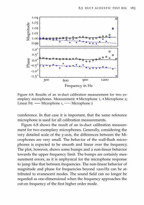
6.5 duct acoustic test rig 163
0.991.001.011.021.031.04
Mag
nitu
de
300 600 900 1200-1.5°-1.0°
-0.5°0.0°
0.5°1.0°
Frequency in Hz
Phas
e
Figure 6.8: Results of an in-duct calibration measurement for two ex-emplary microphones. Measurement: Microphone 1, Microphone 2;Linear Fit: Microphone 1, Microphone 2
cumference. In that case it is important, that the same referencemicrophone is used for all calibration measurements.
Figure 6.8 shows the result of an in-duct calibration measure-ment for two exemplary microphones. Generally, considering thevery detailed scale of the y-axis, the differences between the Mi-crophones are very small. The behavior of the wall-flush micro-phones is expected to be smooth and linear over the frequency.The plot, however, shows some bumps and a non-linear behaviortowards the upper frequency limit. The bumps are certainly mea-surement errors, as it is unphysical for the microphone responseto jump like that between frequencies. The non-linear behavior ofmagnitude and phase for frequencies beyond 1200 Hz can be at-tributed to evanescent modes. The sound field can no longer beregarded as one-dimensional when the frequency approaches thecut-on frequency of the first higher order mode.
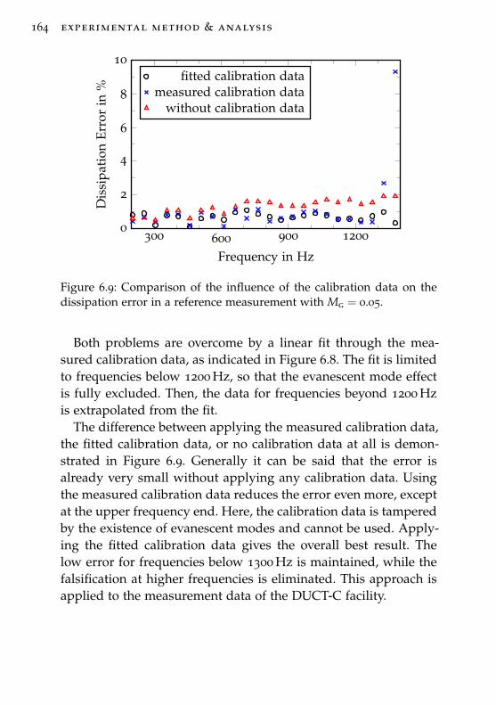
164 experimental method & analysis
300 600 900 12000
2
4
6
8
10
Frequency in Hz
Dis
sipa
tion
Erro
rin
%
fitted calibration datameasured calibration data
without calibration data
Figure 6.9: Comparison of the influence of the calibration data on thedissipation error in a reference measurement with Mg = 0.05.
Both problems are overcome by a linear fit through the mea-sured calibration data, as indicated in Figure 6.8. The fit is limitedto frequencies below 1200 Hz, so that the evanescent mode effectis fully excluded. Then, the data for frequencies beyond 1200 Hzis extrapolated from the fit.
The difference between applying the measured calibration data,the fitted calibration data, or no calibration data at all is demon-strated in Figure 6.9. Generally it can be said that the error isalready very small without applying any calibration data. Usingthe measured calibration data reduces the error even more, exceptat the upper frequency end. Here, the calibration data is tamperedby the existence of evanescent modes and cannot be used. Apply-ing the fitted calibration data gives the overall best result. Thelow error for frequencies below 1300 Hz is maintained, while thefalsification at higher frequencies is eliminated. This approach isapplied to the measurement data of the DUCT-C facility.
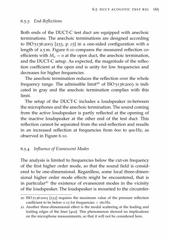
6.5 duct acoustic test rig 165
6.5.3 End-Reflections
Both ends of the DUCT-C test duct are equipped with anechoicterminations. The anechoic terminations are designed accordingto ISO 5136:2003 [233, p. 15] in a one-sided configuration with alength of 2.5 m. Figure 6.10 compares the measured reflection co-efficients with Mg = 0 at the open duct, the anechoic termination,and the DUCT-C setup. As expected, the magnitude of the reflec-tion coefficient at the open end is unity for low frequencies anddecreases for higher frequencies.
The anechoic termination reduces the reflection over the wholefrequency range. The admissible limit20 of ISO 5136:2003 is indi-cated in gray and the anechoic termination complies with thislimit.
The setup of the DUCT-C includes a loudspeaker in-betweenthe microphones and the anechoic termination. The sound comingfrom the active loudspeaker is partly reflected at the opening ofthe inactive loudspeaker at the other end of the test duct. Thisreflection cannot be separated from the end-reflection and resultsin an increased reflection at frequencies from 600 to 900 Hz, asobserved in Figure 6.10.
6.5.4 Influence of Evanescent Modes
The analysis is limited to frequencies below the cut-on frequencyof the first higher order mode, so that the sound field is consid-ered to be one-dimensional. Regardless, some local three-dimen-sional higher order mode effects might be encountered, that isin particular21 the existence of evanescent modes in the vicinityof the loudspeaker. The loudspeaker is mounted to the circumfer-
20 ISO 5136:2003 [233] requires the maximum value of the pressure reflectioncoefficient to be below 0.15 for frequencies > 160 Hz.
21 Another three-dimensional effect is the modal scattering at the leading andtrailing edges of the liner [402]. This phenomenon showed no implicationson the microphone measurements, so that it will not be considered here.
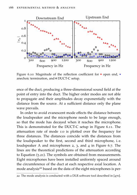
166 experimental method & analysis
300 600 900 12000
0.2
0.4
0.6
0.8
1
Frequency in Hz
|re|
Downstream End
300 600 900 1200
Frequency in Hz
Upstream End
Figure 6.10: Magnitude of the reflection coefficient for open end,anechoic termination, and DUCT-C setup.
ence of the duct, producing a three-dimensional sound field at thepoint of entry into the duct. The higher order modes are not ableto propagate and their amplitudes decay exponentially with thedistance from the source. At a sufficient distance only the planewave prevails.
In order to avoid evanescent mode effects the distance betweenthe loudspeaker and the microphone needs to be large enough,so that the mode has decayed when it reaches the microphone.This is demonstrated for the DUCT-C setup in Figure 6.11. Theattenuation rate of mode 1:0 is plotted over the frequency forthree distances. The distances coincide with the distances fromthe loudspeaker to the first, second and third microphone, i. e.loudspeaker A and microphones 2, 3, and 4 in Figure 6.7. Thelines are the theoretical predictions of the attenuation accordingto Equation (5.21). The symbols are obtained from measurements.Eight microphones have been installed uniformly spaced aroundthe circumference of the duct at each respective axial location. Amode analysis22 based on the data of the eight microphones is per-
22 The mode analysis is conducted with a DLR software tool described in [470].
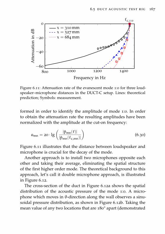
6.5 duct acoustic test rig 167
800 1000 1200 1400−60
−40
−20
0fc,1:0
Frequency in Hz
Att
enua
tion
indB
x = 310 mmx = 527 mmx = 684 mm
Figure 6.11: Attenuation rate of the evanescent mode 1:0 for three loud-speaker–microphone distances in the DUCT-C setup. Lines: theoreticalprediction; Symbols: measurement.
formed in order to identify the amplitude of mode 1:0. In orderto obtain the attenuation rate the resulting amplitudes have beennormalized with the amplitude at the cut-on frequency:
amn = 20 · lg(
|pmn(f)|
|pmn(fc,mn)|
)(6.30)
Figure 6.11 illustrates that the distance between loudspeaker andmicrophone is crucial for the decay of the mode.
Another approach is to install two microphones opposite eachother and taking their average, eliminating the spatial structureof the first higher order mode. The theoretical background to thisapproach, let’s call it double microphone approach, is illustratedin Figure 6.12.
The cross-section of the duct in Figure 6.12a shows the spatialdistribution of the acoustic pressure of the mode 1:0. A micro-phone which moves in θ-direction along the wall observes a sinu-soidal pressure distribution, as shown in Figure 6.12b. Taking themean value of any two locations that are 180° apart (demonstrated
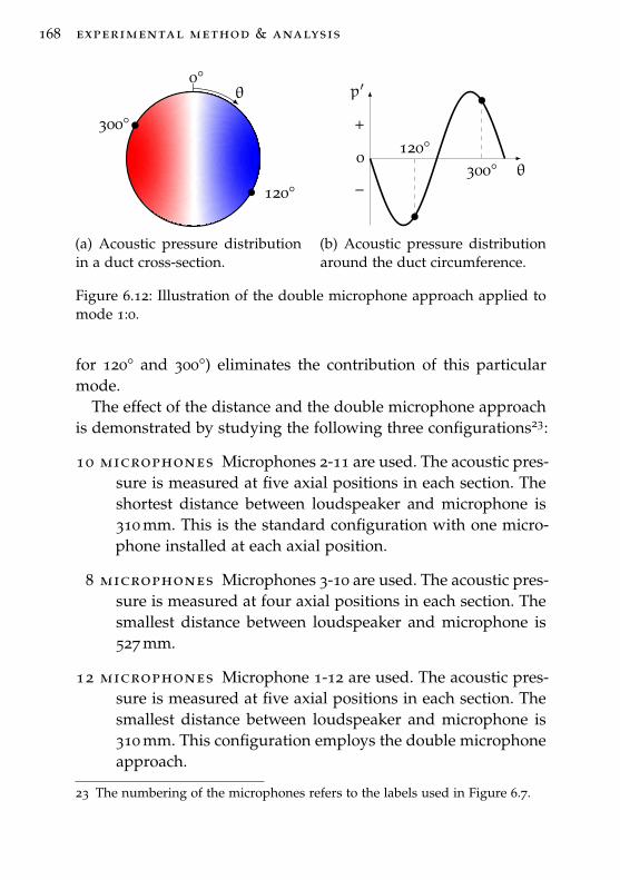
168 experimental method & analysis
θ°0°
120°
300°
(a) Acoustic pressure distributionin a duct cross-section.
θ
p′
−
+
0 120°300°
(b) Acoustic pressure distributionaround the duct circumference.
Figure 6.12: Illustration of the double microphone approach applied tomode 1:0.
for 120° and 300°) eliminates the contribution of this particularmode.
The effect of the distance and the double microphone approachis demonstrated by studying the following three configurations23:
10 microphones Microphones 2-11 are used. The acoustic pres-sure is measured at five axial positions in each section. Theshortest distance between loudspeaker and microphone is310 mm. This is the standard configuration with one micro-phone installed at each axial position.
18 microphones Microphones 3-10 are used. The acoustic pres-sure is measured at four axial positions in each section. Thesmallest distance between loudspeaker and microphone is527 mm.
12 microphones Microphone 1-12 are used. The acoustic pres-sure is measured at five axial positions in each section. Thesmallest distance between loudspeaker and microphone is310 mm. This configuration employs the double microphoneapproach.
23 The numbering of the microphones refers to the labels used in Figure 6.7.
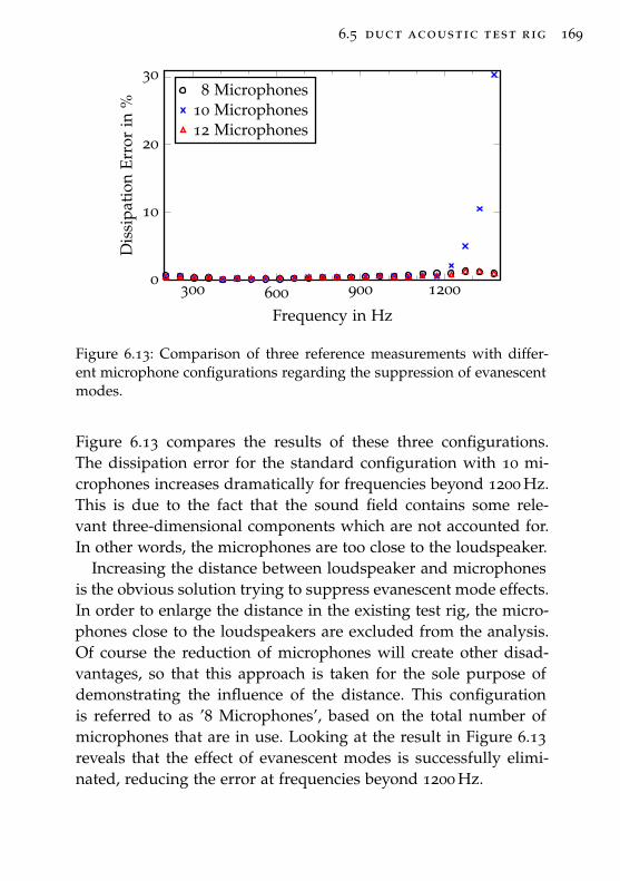
6.5 duct acoustic test rig 169
300 600 900 12000
10
20
30
Frequency in Hz
Dis
sipa
tion
Erro
rin
%
8 Microphones10 Microphones12 Microphones
Figure 6.13: Comparison of three reference measurements with differ-ent microphone configurations regarding the suppression of evanescentmodes.
Figure 6.13 compares the results of these three configurations.The dissipation error for the standard configuration with 10 mi-crophones increases dramatically for frequencies beyond 1200 Hz.This is due to the fact that the sound field contains some rele-vant three-dimensional components which are not accounted for.In other words, the microphones are too close to the loudspeaker.
Increasing the distance between loudspeaker and microphonesis the obvious solution trying to suppress evanescent mode effects.In order to enlarge the distance in the existing test rig, the micro-phones close to the loudspeakers are excluded from the analysis.Of course the reduction of microphones will create other disad-vantages, so that this approach is taken for the sole purpose ofdemonstrating the influence of the distance. This configurationis referred to as ’8 Microphones’, based on the total number ofmicrophones that are in use. Looking at the result in Figure 6.13reveals that the effect of evanescent modes is successfully elimi-nated, reducing the error at frequencies beyond 1200 Hz.
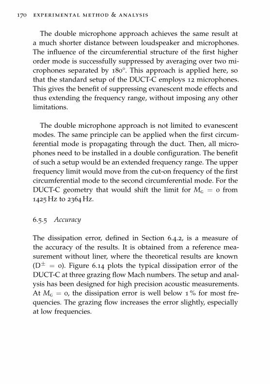
170 experimental method & analysis
The double microphone approach achieves the same result ata much shorter distance between loudspeaker and microphones.The influence of the circumferential structure of the first higherorder mode is successfully suppressed by averaging over two mi-crophones separated by 180°. This approach is applied here, sothat the standard setup of the DUCT-C employs 12 microphones.This gives the benefit of suppressing evanescent mode effects andthus extending the frequency range, without imposing any otherlimitations.
The double microphone approach is not limited to evanescentmodes. The same principle can be applied when the first circum-ferential mode is propagating through the duct. Then, all micro-phones need to be installed in a double configuration. The benefitof such a setup would be an extended frequency range. The upperfrequency limit would move from the cut-on frequency of the firstcircumferential mode to the second circumferential mode. For theDUCT-C geometry that would shift the limit for Mg = 0 from1425 Hz to 2364 Hz.
6.5.5 Accuracy
The dissipation error, defined in Section 6.4.2, is a measure ofthe accuracy of the results. It is obtained from a reference mea-surement without liner, where the theoretical results are known(D± = 0). Figure 6.14 plots the typical dissipation error of theDUCT-C at three grazing flow Mach numbers. The setup and anal-ysis has been designed for high precision acoustic measurements.At Mg = 0, the dissipation error is well below 1 % for most fre-quencies. The grazing flow increases the error slightly, especiallyat low frequencies.
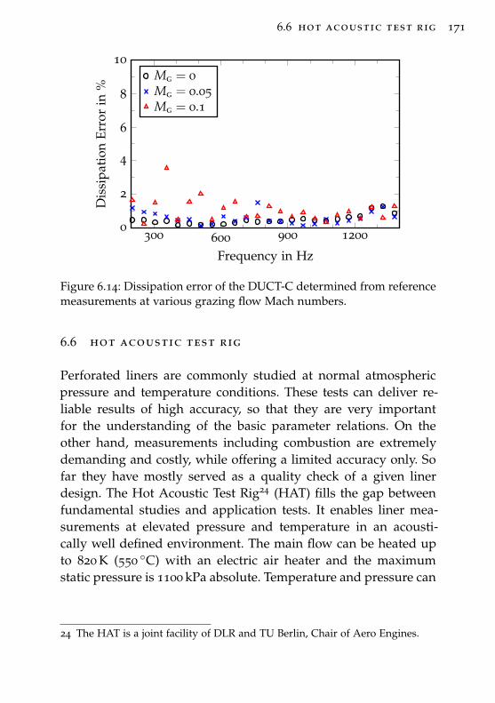
6.6 hot acoustic test rig 171
300 600 900 12000
2
4
6
8
10
Frequency in Hz
Dis
sipa
tion
Erro
rin
%
Mg = 0Mg = 0.05Mg = 0.1
Figure 6.14: Dissipation error of the DUCT-C determined from referencemeasurements at various grazing flow Mach numbers.
6.6 hot acoustic test rig
Perforated liners are commonly studied at normal atmosphericpressure and temperature conditions. These tests can deliver re-liable results of high accuracy, so that they are very importantfor the understanding of the basic parameter relations. On theother hand, measurements including combustion are extremelydemanding and costly, while offering a limited accuracy only. Sofar they have mostly served as a quality check of a given linerdesign. The Hot Acoustic Test Rig24 (HAT) fills the gap betweenfundamental studies and application tests. It enables liner mea-surements at elevated pressure and temperature in an acousti-cally well defined environment. The main flow can be heated upto 820 K (550 ◦C) with an electric air heater and the maximumstatic pressure is 1100 kPa absolute. Temperature and pressure can
24 The HAT is a joint facility of DLR and TU Berlin, Chair of Aero Engines.
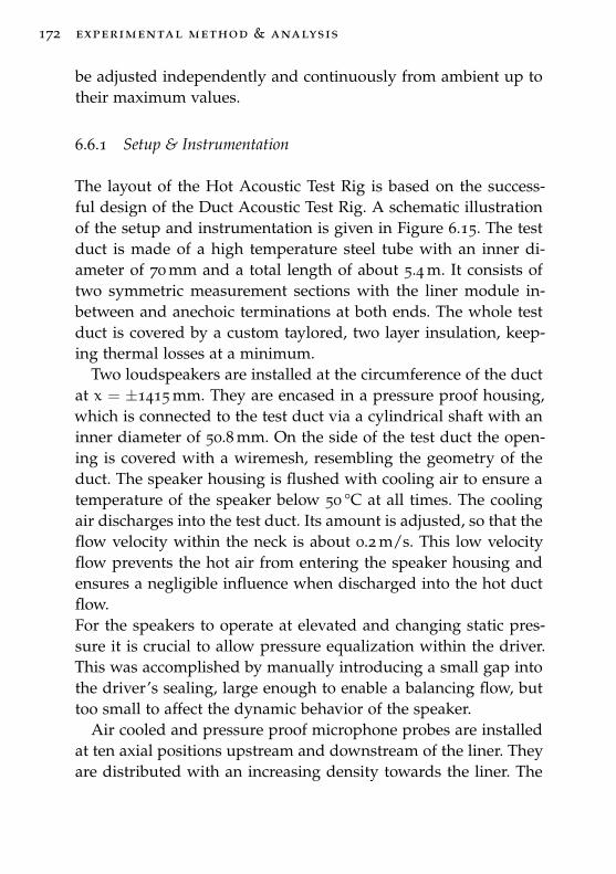
172 experimental method & analysis
be adjusted independently and continuously from ambient up totheir maximum values.
6.6.1 Setup & Instrumentation
The layout of the Hot Acoustic Test Rig is based on the success-ful design of the Duct Acoustic Test Rig. A schematic illustrationof the setup and instrumentation is given in Figure 6.15. The testduct is made of a high temperature steel tube with an inner di-ameter of 70 mm and a total length of about 5.4 m. It consists oftwo symmetric measurement sections with the liner module in-between and anechoic terminations at both ends. The whole testduct is covered by a custom taylored, two layer insulation, keep-ing thermal losses at a minimum.
Two loudspeakers are installed at the circumference of the ductat x = ±1415 mm. They are encased in a pressure proof housing,which is connected to the test duct via a cylindrical shaft with aninner diameter of 50.8 mm. On the side of the test duct the open-ing is covered with a wiremesh, resembling the geometry of theduct. The speaker housing is flushed with cooling air to ensure atemperature of the speaker below 50 °C at all times. The coolingair discharges into the test duct. Its amount is adjusted, so that theflow velocity within the neck is about 0.2 m/s. This low velocityflow prevents the hot air from entering the speaker housing andensures a negligible influence when discharged into the hot ductflow.For the speakers to operate at elevated and changing static pres-sure it is crucial to allow pressure equalization within the driver.This was accomplished by manually introducing a small gap intothe driver’s sealing, large enough to enable a balancing flow, buttoo small to affect the dynamic behavior of the speaker.
Air cooled and pressure proof microphone probes are installedat ten axial positions upstream and downstream of the liner. Theyare distributed with an increasing density towards the liner. The
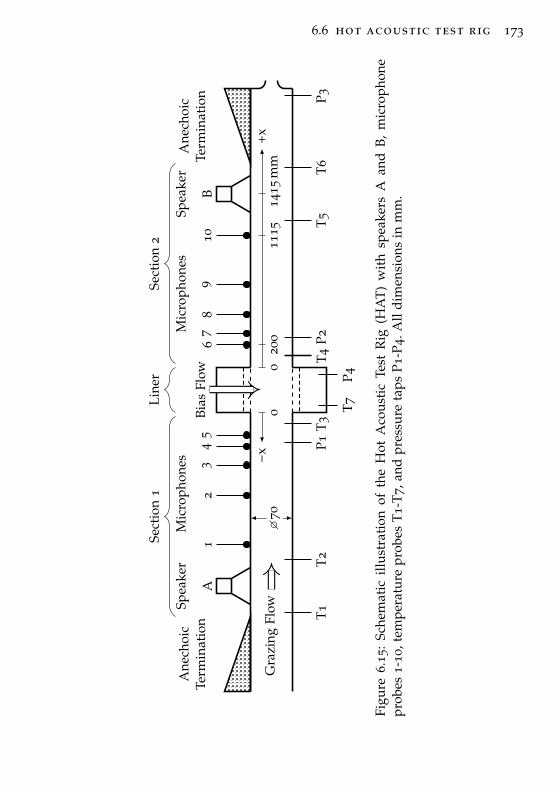
6.6 hot acoustic test rig 173
Ane
choi
cT e
rmin
atio
n
Line
r
A
Spea
ker
54
32
1
Mic
roph
ones
p
Sect
ion
1
Ane
choi
cT e
rmin
atio
nB
Spea
ker
67
89
10
Mic
roph
ones
p
Sect
ion
2
T1T2
T3T
4T5
T6
T7
P1P2
P3
P4
Gra
zing
Flow
Bias
Flow
+−x
0+x
020
0m
m14
15m
m11
15�7
0
Figu
re6.
15:
Sche
mat
icill
ustr
atio
nof
the
Hot
Aco
usti
cTe
stR
ig(H
AT
)w
ith
spea
kers
Aan
dB,
mic
roph
one
prob
es1-
10,t
empe
ratu
repr
obes
T1-T
7,an
dpr
essu
reta
psP1
-P4.
All
dim
ensi
ons
inm
m.
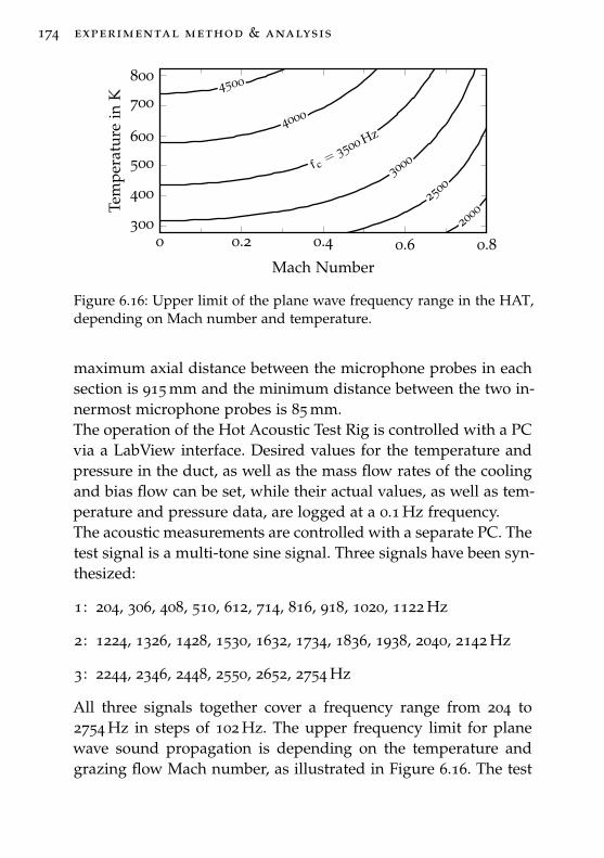
174 experimental method & analysis
0 0.2 0.4 0.6 0.8300
400
500
600
700
800
20002500
3000fc= 3500 Hz
4000
4500
Mach Number
Tem
pera
ture
inK
Figure 6.16: Upper limit of the plane wave frequency range in the HAT,depending on Mach number and temperature.
maximum axial distance between the microphone probes in eachsection is 915 mm and the minimum distance between the two in-nermost microphone probes is 85 mm.The operation of the Hot Acoustic Test Rig is controlled with a PCvia a LabView interface. Desired values for the temperature andpressure in the duct, as well as the mass flow rates of the coolingand bias flow can be set, while their actual values, as well as tem-perature and pressure data, are logged at a 0.1 Hz frequency.The acoustic measurements are controlled with a separate PC. Thetest signal is a multi-tone sine signal. Three signals have been syn-thesized:
1 : 204, 306, 408, 510, 612, 714, 816, 918, 1020, 1122 Hz
2 : 1224, 1326, 1428, 1530, 1632, 1734, 1836, 1938, 2040, 2142 Hz
3 : 2244, 2346, 2448, 2550, 2652, 2754 Hz
All three signals together cover a frequency range from 204 to2754 Hz in steps of 102 Hz. The upper frequency limit for planewave sound propagation is depending on the temperature andgrazing flow Mach number, as illustrated in Figure 6.16. The test
6.6 hot acoustic test rig 175
signal is generated by an Agilent 33220A function generator. Thesignals are fed through a KME SPA240E stereo amplifier, whichpowers two Monacor KU-516 speakers.
The acoustic pressure is recorded over a time of 30 s with a 16track OROS OR36 data acquisition system with a sampling fre-quency of 8192 Hz. Additionally, the output signal of the functiongenerator is recorded at the same settings as a reference signal forthe analysis.
Temperature measurements
The temperature of the main flow is measured at six positionsalong the duct, that is upstream and downstream of each loud-speaker and upstream and downstream of the liner (see T1-T6 inFigure 6.15). The temperature of the bias flow is measured in thecavity of the liner (see T7 in Figure 6.15). Additionally, there is atemperature sensor installed in each speaker housing for healthmonitoring (not shown in Figure 6.15). The sensors are resistivetemperature detectors (RTD) of type PT100 connected in four-wireconfiguration to a digital multimeter (Agilent AG34972). Their ac-curacy is specified as ±0.5°C for the complete temperature rangeof 280-820 K.The analysis of the acoustic data requires an accurate knowledgeof the temperature, as well as a constant temperature along themeasurement sections. The placement of the temperature sensorsallows the assessment of temperature changes along the duct. In-sufficient insulation would produce a continuous temperature gra-dient, while the injection of cooling air through the microphoneprobes, the speaker housing and the liner would cause a suddenchange of temperature. Several tests have been made and it can beconcluded that the temperature gradient due to insufficient insu-lation is negligible, as well as the discharge of cooling air throughthe microphone probes and loudspeaker housings. However, theamount of bias flow can be substantial, so that the temperaturein the downstream section can be much lower than the temper-
176 experimental method & analysis
ature in the upstream section. The actual temperature differencedepends on the initial temperature, and the ratio of grazing andbias flow. In extreme cases the temperature difference between sec-tion 1 and 2 can be as much as 160 K. The change in temperatureis unproblematic as long as the temperatures of both sections areknown and considered separately in the acoustic analysis. Thetemperature of the upstream section serves as the characteristictemperature of a test point.
Static pressure measurements
The static pressure is measured using pressure taps. They are lo-cated upstream and downstream of the liner (see P1 and P2 inFigure 6.15), at the nozzle (see P3 in Figure 6.15) and at variouspositions in the liner cavity (see P4 in Figure 6.15). For redun-dancy there are two pressure taps at each location. While the aver-age value is used for post-processing, the difference between bothvalues serves as an accuracy indicator. The pressure taps are con-nected to two modules of PSI (Pressure Systems, Inc.) 9116 pres-sure scanners. They have separate sensors for absolute and differ-ential pressure measurements and are divided into four blocks ofdifferent pressure ranges: 2.5, 5, 69, and 1380 kPa. The accuracy isdependent on the full scale (FS) value of the range and is specifiedas ±0.05 % FS for the 2.5 and 5 kPa ranges and ±0.15 % FS for thelarger ranges.The pressure in the duct is given as absolute value, while the pres-sure in the liner cavity is given as the differential pressure refer-ring to the absolute pressure in the duct. The pressure in the linercavity is measured at three different radial positions. This enablesthe measurement of the pressure drop over each layer of a doubleskin configuration. In fact, the measured quantities include thepressure drop of the innermost liner and the total pressure dropacross both layers. The third pressure tap enables the measure-ment of the pressure drop in a triple skin configuration. However,until now all measurements dealt with double skin configurations
6.6 hot acoustic test rig 177
only, so that the two outermost pressure taps measured the samepressure.
6.6.2 Air Supply
The air for the HAT facility is provided by two rotary screw com-pressors that can deliver a total mass flow rate of 0.78 kg/s. Theair is dried (at a dew point of 276 K), filtered, and then deliveredinto a 2 m3 pressure reservoir at a temperature of 288 K at 1600 kPaof pressure. The liner bias flow, the microphone cooling flow, andthe speaker cooling flow are delivered at these conditions. Thesupply for each consumer can be set individually via mass flowcontrollers.The main duct flow is fed through an electrical air heater before itenters the duct. The air heater can increase the temperature of theflow to any value between ambient and 820 K. It is custom madeby DLR and has a maximum power rating of 540 kW.The flow rate and pressure in the duct is controlled via a pres-sure valve, a volume flow meter, and a nozzle at the end of thetest duct. The pressure in the duct can be adjusted continuouslybetween ambient and 1100 kPa absolute pressure. The resultingflow velocity in the duct is defined by the geometry of the nozzleand can be determined by the laws of gas dynamics. Raising thepressure in the duct increases the flow velocity until a critical pres-sure is reached. At the critical pressure the velocity in the nozzleequals the speed of sound M = 1. For pressures beyond the criti-cal pressure the velocity remains constant.
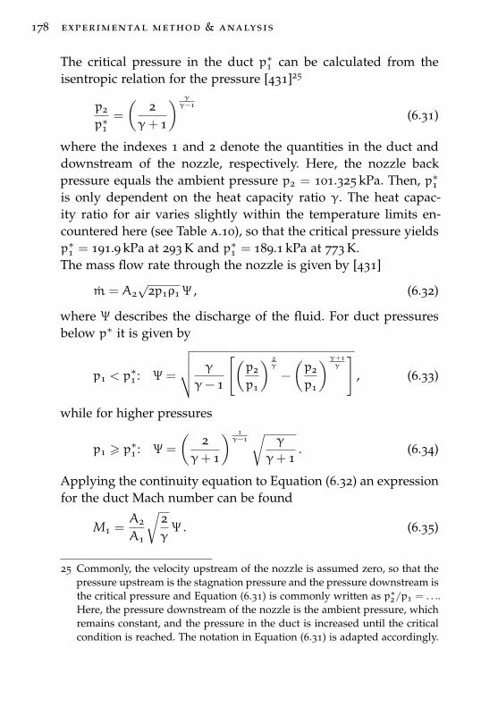
178 experimental method & analysis
The critical pressure in the duct p∗1 can be calculated from theisentropic relation for the pressure [431]25
p2
p∗1=
(2
γ+ 1
) γγ−1
(6.31)
where the indexes 1 and 2 denote the quantities in the duct anddownstream of the nozzle, respectively. Here, the nozzle backpressure equals the ambient pressure p2 = 101.325 kPa. Then, p∗1is only dependent on the heat capacity ratio γ. The heat capac-ity ratio for air varies slightly within the temperature limits en-countered here (see Table a.10), so that the critical pressure yieldsp∗1 = 191.9 kPa at 293 K and p∗1 = 189.1 kPa at 773 K.The mass flow rate through the nozzle is given by [431]
m = A2√
2p1ρ1 Ψ , (6.32)
where Ψ describes the discharge of the fluid. For duct pressuresbelow p∗ it is given by
p1 < p∗1 : Ψ =
√√√√ γ
γ− 1
[(p2
p1
) 2γ
−
(p2
p1
)γ+1γ
], (6.33)
while for higher pressures
p1 > p∗1 : Ψ =
(2
γ+ 1
) 1γ−1√
γ
γ+ 1. (6.34)
Applying the continuity equation to Equation (6.32) an expressionfor the duct Mach number can be found
M1 =A2
A1
√2γΨ . (6.35)
25 Commonly, the velocity upstream of the nozzle is assumed zero, so that thepressure upstream is the stagnation pressure and the pressure downstream isthe critical pressure and Equation (6.31) is commonly written as p∗2/p1 = . . ..Here, the pressure downstream of the nozzle is the ambient pressure, whichremains constant, and the pressure in the duct is increased until the criticalcondition is reached. The notation in Equation (6.31) is adapted accordingly.
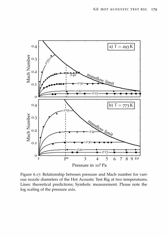
6.6 hot acoustic test rig 179
�15�20
�30
�40
�55
massflow limit
a) T = 293 K
0
0.1
0.2
0.3
0.4
Mac
hN
umbe
r
�15�20
�30
�40
�55
massflow limit
b) T = 773 K
1 P*... 3 4 5 6 7 8 9 100
0.1
0.2
0.3
0.4
Pressure in 105 Pa
Mac
hN
umbe
r
Figure 6.17: Relationship between pressure and Mach number for vari-ous nozzle diameters of the Hot Acoustic Test Rig at two temperatures.Lines: theoretical predictions; Symbols: measurement. Please note thelog scaling of the pressure axis.
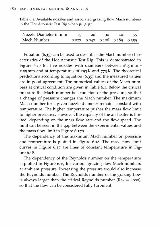
180 experimental method & analysis
Table 6.1: Available nozzles and associated grazing flow Mach numbersin the Hot Acoustic Test Rig when p1 > p∗1 .
Nozzle Diameter in mm 15 20 30 40 55Mach Number 0.027 0.047 0.106 0.189 0.359
Equation (6.35) can be used to describes the Mach number char-acteristics of the Hot Acoustic Test Rig. This is demonstrated inFigure 6.17 for five nozzles with diameters between �15 mm -�55 mm and at temperatures of 293 K and 773 K. The theoreticalpredictions according to Equation (6.35) and the measured valuesare in good agreement. The numerical values of the Mach num-bers at critical condition are given in Table 6.1. Below the criticalpressure the Mach number is a function of the pressure, so thata change of pressure changes the Mach number. The maximumMach number for a given nozzle diameter remains constant withtemperature. The higher temperature pushes the mass flow limitto higher pressures. However, the capacity of the air heater is lim-ited, depending on the mass flow rate and the flow speed. Thelimit can be seen in the gap between the experimental values andthe mass flow limit in Figure 6.17b.
The dependency of the maximum Mach number on pressureand temperature is plotted in Figure 6.18. The mass flow limitcurves in Figure 6.17 are lines of constant temperature in Fig-ure 6.18.
The dependency of the Reynolds number on the temperatureis plotted in Figure 6.19 for various grazing flow Mach numbersat ambient pressure. Increasing the pressure would also increasethe Reynolds number. The Reynolds number of the grazing flowis always larger than the critical Reynolds number (Rec = 4000),so that the flow can be considered fully turbulent.
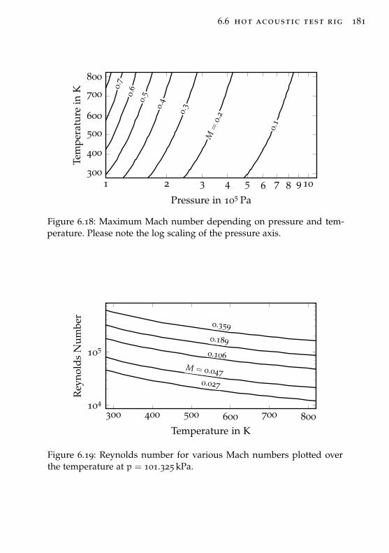
6.6 hot acoustic test rig 181
1 2 3 4 5 6 7 8 9 10300
400
500
600
700
800
0.1
M=
0.20.
30.40.
50.60.
7
Pressure in 105 Pa
Tem
pera
ture
inK
Figure 6.18: Maximum Mach number depending on pressure and tem-perature. Please note the log scaling of the pressure axis.
300 400 500 600 700 800104
105
0.027
M = 0.047
0.106
0.189
0.359
Temperature in K
Rey
nold
sN
umbe
r
Figure 6.19: Reynolds number for various Mach numbers plotted overthe temperature at p = 101.325 kPa.
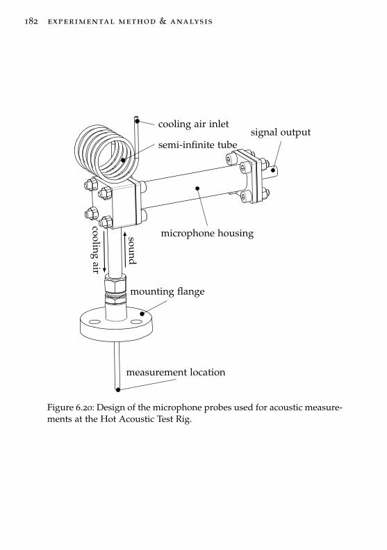
182 experimental method & analysis
draft – 2014.06.17 16:15 – claus lahiri
Isometric viewScale: 1:1
signal outputcooling air inlet
semi-infinite tube
microphone housing
mounting flange
measurement location
sound
coolingair
Figure 6.20: Design of the microphone probes used for acoustic measure-ments at the Hot Acoustic Test Rig.
6.6 hot acoustic test rig 183
6.6.3 Microphone Probes
Accurate acoustic measurements in high temperature flow arevery challenging. Commercial products are typically based on apiezoelectric sensor. Their maximum tolerable temperature is typ-ically around 620 K (in a very few cases the specifications go ashigh as 920 K). However, the sensitivity of piezoelectric pressuresensors is much lower compared to a standard condenser micro-phone. In order to overcome this limitation a microphone probehas been developed at DLR. The original design has been usedsuccessfully for several years, e. g. for acoustic measurements in alaboratory combustion chamber. Recently, the design has receiveda major upgrade to include the ability of measuring in high pres-sure environments of up to 2000 kPa. The microphone probes havebeen successfully tested in a combustion facility with respect totheir safety and data reproducibility at conditions up to 1350 kPaand 1500 K.
The design of the microphone probes is shown in Figure 6.20.The probes are mounted to the test duct via a flange. The tubebelow the flange is inserted into the wall of the test duct, so thatthe end of the tube is flush with the wall. This is the measure-ment location where the acoustic pressure is to be recorded. Thetube extends outwards with a constant diameter. After a certainlength a microphone is mounted perpendicular to the tube in-side a pressure-proof housing. The housing contains a standardquarter-inch condenser microphone (G.R.A.S. 40BP or 40BH) andits pre-amplifier (G.R.A.S. 26AC). The acoustic signal is transmit-ted from the tube to the microphone membrane via a small open-ing. The microphone signal is passed on through the wall with apressure-proof wall bushing that ends in a LEMO connector.In order to prevent reflections of sound, the tube is extended be-yond the location of the microphone, following the principle of asemi-infinite tube. The overall length of this tube is about one me-ter which is mostly wound-up in a spiral to save space. The large
184 experimental method & analysis
ratio between diameter and length of the tube provides sufficientviscous damping, so that the frequency range of interest is freefrom resonances.A small amount of cooling air is fed through the tube, prevent-ing hot gases from the duct to enter the tube and get into contactwith the microphone membrane. A study regarding the influenceof the cooling flow on the acoustic measurement was done withthe initial design of the microphone probes (unpublished). At at-mospheric pressure it was shown that a velocity of 4 m/s in thetube is enough to ensure the safe operation of the microphones.This corresponds to a mass flow rate of 0.054 kg/h at atmosphericconditions. The required value for the cooling flow velocity is heldconstant at elevated pressures, so that the mass flow rate has tobe adjusted according to the change in density. A disturbance ofthe signal by the cooling air could only be observed for velocitiesbeyond 30 m/s.
Each microphone probe has a characteristic transfer functionwhich is determined by the geometric dimensions of the probe,i. e. the diameter of the tube, the distance between the measure-ment location and the microphone membrane, etc. The transferfunction has to be considered in the analysis, correcting the sig-nals from the transfer characteristics of the probe. While the speci-fied geometry is identical for all probes, so should be their transferfunctions. However, small variation in manufacturing and assem-bly require the determination of an individual transfer functionfor each probe.A probe together with a microphone is forming one unit, whichis only separated if a component is damaged. Instead of deter-mining the transfer function of the probe separately, a calibrationcurve for the whole unit is determined. Then, the calibration curveincludes the transfer function of the probe as well as the behaviorof the microphone itself. Three different ways of calibration havebeen established:
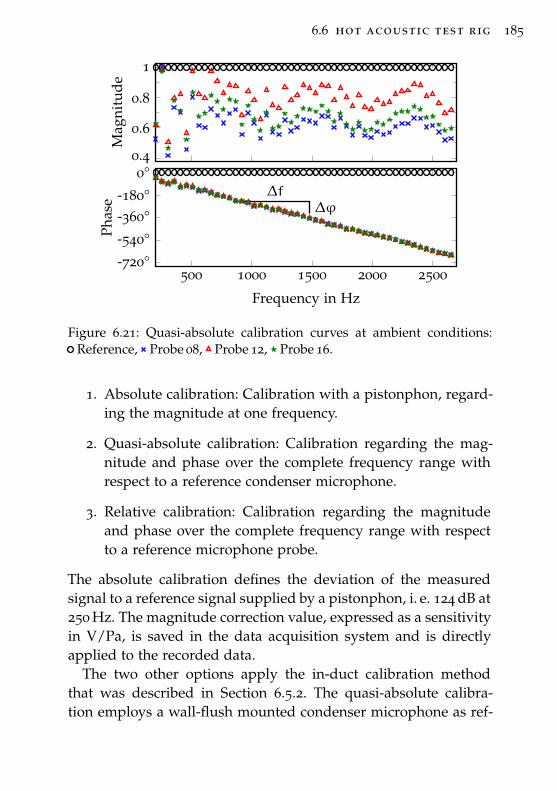
6.6 hot acoustic test rig 185
0.4
0.6
0.8
1
Mag
nitu
de
∆f∆ϕ
500 1000 1500 2000 2500-720°
-540°
-360°-180°
0°
Frequency in Hz
Phas
e
Figure 6.21: Quasi-absolute calibration curves at ambient conditions:Reference, Probe 08, Probe 12, Probe 16.
1. Absolute calibration: Calibration with a pistonphon, regard-ing the magnitude at one frequency.
2. Quasi-absolute calibration: Calibration regarding the mag-nitude and phase over the complete frequency range withrespect to a reference condenser microphone.
3. Relative calibration: Calibration regarding the magnitudeand phase over the complete frequency range with respectto a reference microphone probe.
The absolute calibration defines the deviation of the measuredsignal to a reference signal supplied by a pistonphon, i. e. 124 dB at250 Hz. The magnitude correction value, expressed as a sensitivityin V/Pa, is saved in the data acquisition system and is directlyapplied to the recorded data.
The two other options apply the in-duct calibration methodthat was described in Section 6.5.2. The quasi-absolute calibra-tion employs a wall-flush mounted condenser microphone as ref-
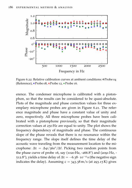
186 experimental method & analysis
0.6
0.8
1.0
1.2
Mag
nitu
de
500 1000 1500 2000 2500
-20°
-10°
0°
Frequency in Hz
Phas
e
Figure 6.22: Relative calibration curves at ambient conditions: Probe 04(Reference), Probe 08, Probe 12, Probe 16.
erence. The condenser microphone is calibrated with a piston-phon, so that the results can be considered to be quasi-absolute.Plots of the magnitude and phase correction values for three ex-emplary microphone probes are given in Figure 6.21. The refer-ence magnitude and phase have a constant value of unity andzero, respectively. All three microphone probes have been cali-brated with a pistonphone previously, so that their magnitudecorrection values at 250 Hz are equal to unity. The plot shows thefrequency dependency of magnitude and phase. The continuousslope of the phase reveals that there is no resonance within thefrequency range. The slope itself defines the time delay of theacoustic wave traveling from the measurement location to the mi-crophone: ∆t = ∆ϕ/360°/∆f. Picking two random points fromthe phase curve of probe 16, say (1020 Hz, -266.8°) and (2091 Hz, -512.8°), yields a time delay of ∆t = −6.38 ·10−4 s (the negative signindicates the delay). Assuming c = 343.38 m/s (at 293.15 K) gives
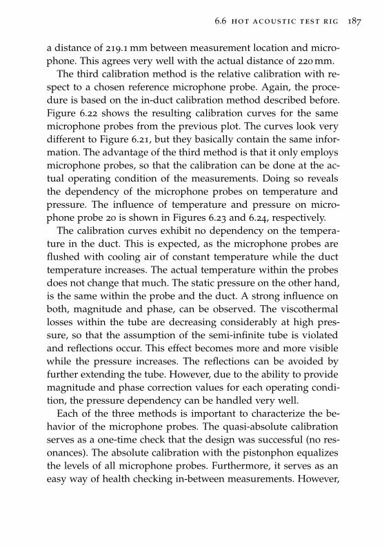
6.6 hot acoustic test rig 187
a distance of 219.1 mm between measurement location and micro-phone. This agrees very well with the actual distance of 220 mm.
The third calibration method is the relative calibration with re-spect to a chosen reference microphone probe. Again, the proce-dure is based on the in-duct calibration method described before.Figure 6.22 shows the resulting calibration curves for the samemicrophone probes from the previous plot. The curves look verydifferent to Figure 6.21, but they basically contain the same infor-mation. The advantage of the third method is that it only employsmicrophone probes, so that the calibration can be done at the ac-tual operating condition of the measurements. Doing so revealsthe dependency of the microphone probes on temperature andpressure. The influence of temperature and pressure on micro-phone probe 20 is shown in Figures 6.23 and 6.24, respectively.
The calibration curves exhibit no dependency on the tempera-ture in the duct. This is expected, as the microphone probes areflushed with cooling air of constant temperature while the ducttemperature increases. The actual temperature within the probesdoes not change that much. The static pressure on the other hand,is the same within the probe and the duct. A strong influence onboth, magnitude and phase, can be observed. The viscothermallosses within the tube are decreasing considerably at high pres-sure, so that the assumption of the semi-infinite tube is violatedand reflections occur. This effect becomes more and more visiblewhile the pressure increases. The reflections can be avoided byfurther extending the tube. However, due to the ability to providemagnitude and phase correction values for each operating condi-tion, the pressure dependency can be handled very well.
Each of the three methods is important to characterize the be-havior of the microphone probes. The quasi-absolute calibrationserves as a one-time check that the design was successful (no res-onances). The absolute calibration with the pistonphon equalizesthe levels of all microphone probes. Furthermore, it serves as aneasy way of health checking in-between measurements. However,
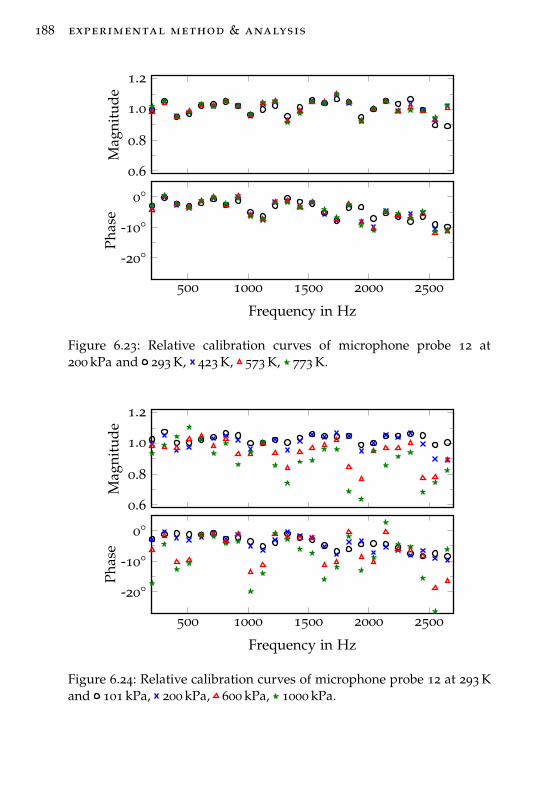
188 experimental method & analysis
0.6
0.8
1.0
1.2
Mag
nitu
de
500 1000 1500 2000 2500
-20°
-10°
0°
Frequency in Hz
Phas
e
Figure 6.23: Relative calibration curves of microphone probe 12 at200 kPa and 293 K, 423 K, 573 K, 773 K.
0.6
0.8
1.0
1.2
Mag
nitu
de
500 1000 1500 2000 2500
-20°
-10°
0°
Frequency in Hz
Phas
e
Figure 6.24: Relative calibration curves of microphone probe 12 at 293 Kand 101 kPa, 200 kPa, 600 kPa, 1000 kPa.
6.6 hot acoustic test rig 189
it should be noted that applying a new absolute calibration valuemakes any previous relative calibration invalid (the magnitudecurve will have an offset). The relative calibration at operatingcondition is crucial for the analysis of the data. Therefore, a rel-ative calibration is performed in regular intervals, at least at thebeginning of a measurement campaign.
6.6.4 Estimation of the Humidity
The treatment of the acoustic losses at elevated pressure and tem-perature in the next section requires some knowledge about thehumidity. The relevant quantity for the acoustic losses is the mo-lar concentration of water vapor h (fraction of air molecules thatare water). The air provided for the Hot Acoustic Test Rig isdried at a dew point temperature Td = 276.15 K (3 °C) at an op-erating pressure of 1500 kPa. The saturation pressure at the dewpoint temperature is calculated from Equation (5.64) and results inpws (Td) = 758.054 Pa. The relative humidity in the saturated stateis RH = 100 %, so that the molar concentration of water vapor isgiven by Equation (5.63) as h = 0.051 %. The molar concentrationis determined by the operating conditions of the air dryer. Thetemperature in the Hot Acoustic Test Rig is always well above thedew point temperature and the pressure is always well below thesaturation pressure at the respective temperature, so that the mo-lar concentration of water vapor in the air stays constant and isindependent of the operating temperature and pressure.
The relative humidity might be the more well-known quantity.It can be calculated from Equation (5.63) with h = 0.051 %, thesaturation pressure at operating temperature pws (T), and the op-erating pressure p. Its values range from 32.9 % (at 288.15 K and1100 kPa) to 0.0002 % (at the critical temperature Tc = 647.096 Kand 101.325 kPa), while it is 4 % at ISA conditions (288.15 K and101.325 kPa).
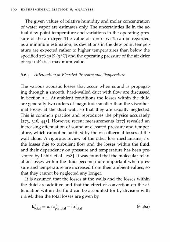
190 experimental method & analysis
The given values of relative humidity and molar concentrationof water vapor are estimates only. The uncertainties lie in the ac-tual dew point temperature and variations in the operating pres-sure of the air dryer. The value of h = 0.051 % can be regardedas a minimum estimation, as deviations in the dew point temper-ature are expected rather to higher temperatures than below thespecified 276.15 K (3 °C) and the operating pressure of the air drierof 1500 kPa is a maximum value.
6.6.5 Attenuation at Elevated Pressure and Temperature
The various acoustic losses that occur when sound is propagat-ing through a smooth, hard-walled duct with flow are discussedin Section 5.4. At ambient conditions the losses within the fluidare generally two orders of magnitude smaller than the viscother-mal losses at the duct wall, so that they are usually neglected.This is common practice and reproduces the physics accurately[273, 316, 445]. However, recent measurements [277] revealed anincreasing attenuation of sound at elevated pressure and temper-ature, which cannot be justified by the viscothermal losses at thewall alone. A rigorous review of the other loss mechanisms, i. e.the losses due to turbulent flow and the losses within the fluid,and their dependency on pressure and temperature has been pre-sented by Lahiri et al. [278]. It was found that the molecular relax-ation losses within the fluid become more important when pres-sure and temperature are increased from their ambient values, sothat they cannot be neglected any longer.
It is assumed that the losses at the walls and the losses withinthe fluid are additive and that the effect of convection on the at-tenuation within the fluid can be accounted for by division with1±M, then the total losses are given by
k±total = ω/c±ph,total − iα±total (6.36a)

6.6 hot acoustic test rig 191
with the attenuation coefficient and phase velocity given by
α±total = αfluid/(1±M) +α±turb and (6.36b)
c±ph,total = (c+∆cph,fluid +∆c±ph,turb)(1±M) . (6.36c)
The total losses include the viscothermal losses within the fluid,the losses due to rotational and vibrational molecular relaxation,the viscothermal losses at the duct wall, the convective effect ofthe flow on the wall losses, and the absorption due to the turbu-lent flow boundary-layer. The respective equations for αfluid, α±turb,∆cph,fluid, and ∆c±ph,turb are given in Section 5.4.
The attenuation coefficient at elevated pressure and tempera-ture has been determined experimentally with the Hot AcousticTest Rig. Details of the measurements can be found in [278]. Fig-ure 6.25 shows a comparison between the experimental data andthe theoretical predictions of Equation (6.36b). The convective in-fluence of the flow on α±total is small, so that only the average valueαtotal = (α+
total +α−total)/2 is plotted.
While there is some scatter in the experimental data, it matchesthe theoretical predictions rather well. Setting h = 0.08 % for themodel matches the experimental data slightly better than the es-timate h = 0.051 %. This corresponds, for example, to a changeof operating condition of the air dryer to 280.65 K and 1300 kPa,which is a valid assumption.
According to Equation (6.36b), the total losses are the superposi-tion of αfluid and α±turb, which are also plotted in Figure 6.25. α±turbis mostly determined by the viscothermal losses at the duct wall,except at low frequencies where the losses due to the turbulentflow boundary-layer become prominent. However, the attenuationin the measured frequency range (indicated in gray) is dominatedby the losses within the fluid at both operating conditions.
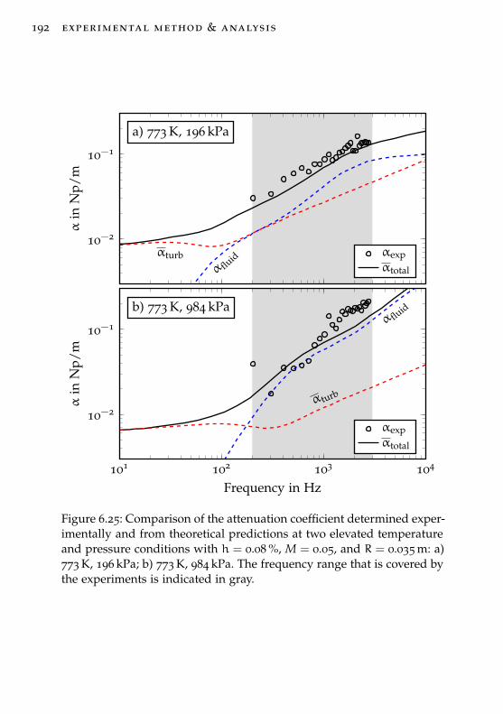
192 experimental method & analysis
α fluidαturb
a) 773 K, 196 kPa
10−2
10−1
αin
Np/
m
αexpαtotal
α fluid
α turb
b) 773 K, 984 kPa
101 102 103 104
10−2
10−1
Frequency in Hz
αin
Np/
m
αexpαtotal
Figure 6.25: Comparison of the attenuation coefficient determined exper-imentally and from theoretical predictions at two elevated temperatureand pressure conditions with h = 0.08 %, M = 0.05, and R = 0.035 m: a)773 K, 196 kPa; b) 773 K, 984 kPa. The frequency range that is covered bythe experiments is indicated in gray.
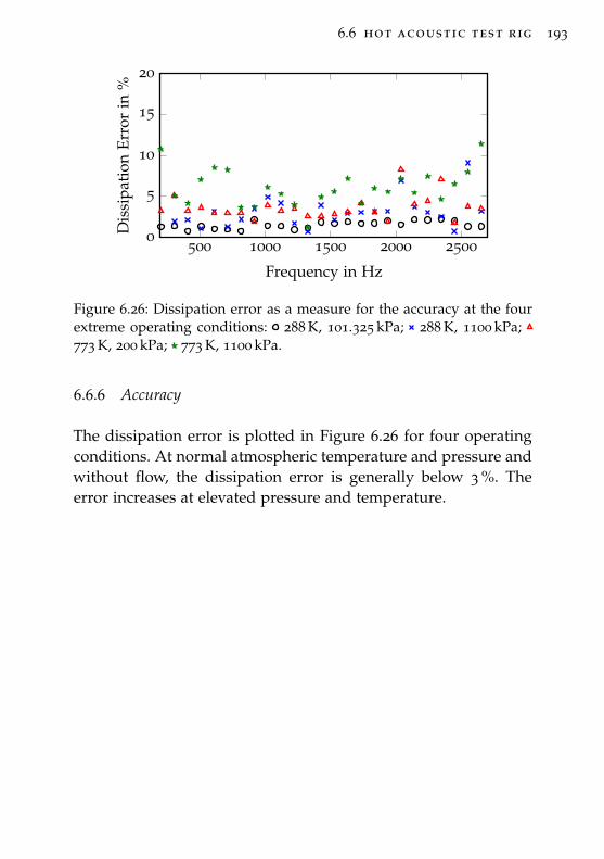
6.6 hot acoustic test rig 193
500 1000 1500 2000 25000
5
10
15
20
Frequency in Hz
Dis
sipa
tion
Erro
rin
%
Figure 6.26: Dissipation error as a measure for the accuracy at the fourextreme operating conditions: 288 K, 101.325 kPa; 288 K, 1100 kPa;773 K, 200 kPa; 773 K, 1100 kPa.
6.6.6 Accuracy
The dissipation error is plotted in Figure 6.26 for four operatingconditions. At normal atmospheric temperature and pressure andwithout flow, the dissipation error is generally below 3 %. Theerror increases at elevated pressure and temperature.

7PA R A M E T E R S T U D Y
This chapter presents the results of the experimental parameterstudy. Each parameter is addressed individually, always includinga bias flow. The text presents a selection of results of significant im-portance. The geometric specifications of the liner configurationsare listed in Table 7.1.
7.1 sound pressure level
The amplitude of the acoustic oscillations in a gas turbine com-bustor can be very high, especially when instabilities occur. Thissection studies the effect of high amplitudes on the dissipation ofsound at perforations with and without bias flow.
Various definitions of the measured amplitude are discussedin Section 2.4.2. Here, a combination of the incident wave ampli-tude and the fixed reference location method is applied. The loud-speaker output is adjusted to match a nominal SPL at a referencemicrophone in the hard-walled duct section. The measurement isperformed with this nominal SPL value. In the analysis, the inci-dent wave amplitude is determined from a wave decompositionand used for the presentation of the data. The combination ofthese two methods eliminates the time consuming adjustment tomatch a certain SPLvalue. As a result, the actual SPL values arescattering slightly around the nominal values.
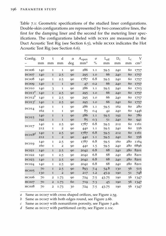
196 parameter study
Table 7.1: Geometric specifications of the studied liner configurations.Double-skin configurations are represented by two consecutive lines, thefirst for the damping liner and the second for the metering liner spec-ifications. The configurations labeled with dcxxx are measured in theDuct Acoustic Test Rig (see Section 6.5), while hcxxx indicates the HotAcoustic Test Rig (see Section 6.6).
Config. D t d α Aopen σ Leff Dc Lc V
– mm mm mm deg mm2 % mm mm mm cm3
dc006 140 1 1 90 286 1.1 59.5 240 60 1757dc007 140 1 2.5 90 295 1.0 66 240 60 1757dc008 140 1 2.5 90 1787 6.8 59.5 240 60 1757dc009 140 1 1 90 47 0.2 66 240 60 1757dc010 140 3 1 90 286 1.1 59.5 240 60 1703dc011a 140 1 2.5 90 295 1.0 66 240 60 1757dc012b 140 1 2.5 90 295 1.0 66 240 60 1757dc013c 140 1 2.5 90 295 1.0 66 240 60 1757
140 1 1 90 286 1.1 59.5 162 60 280dc014162 1 1 90 85 0.4 42 240 60 1446140 1 1 90 286 1.1 59.5 192 60 780dc015192 1 1 90 85 0.3 51 240 60 941140 1 2.5 90 1787 6.8 59.5 212 60 1161dc017212 1 2 90 440 1.1 59.5 240 60 556140 1 2.5 90 1787 6.8 59.5 212 60 1161dc018d212 1 2 90 440 1.1 59.5 240 60 556140 1 2.5 90 1787 6.8 59.5 160 280 1164dc019160 1 2 90 440 1.5 59.5 240 280 6896
dc021 140 1 2.5 90 2042 6.8 68 240 280 8201dc022 140 1 2.5 90 2042 6.8 68 240 280 8201dc023 140 1 2.5 90 2042 6.8 68 240 280 8201dc024 140 1 2.5 90 2042 6.8 68 240 280 8201
70 1 2.5 90 893 7.4 54.8 130 56 515hc005130 1 2 90 217 1.2 45.9 190 51 748
hc006 70 2 1.73 90 724 7.5 43.75 190 56 1347hc007 70 2 1.73 60 719 7.3 45 190 56 1347hc008 70 2 1.73 30 724 7.5 43.75 190 56 1347
a Same as dc007 with cross shaped orifices, see Figure 2.5g.b Same as dc007 with both edges round, see Figure 2.6b.c Same as dc007 with nonuniform porosity, see Figure 7.40b.d Same as dc017 with partitioned cavity, see Figure 2.10c.
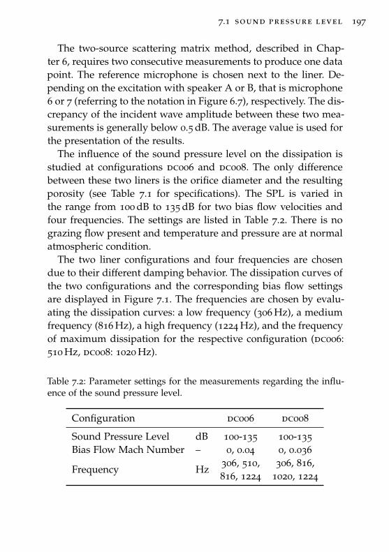
7.1 sound pressure level 197
The two-source scattering matrix method, described in Chap-ter 6, requires two consecutive measurements to produce one datapoint. The reference microphone is chosen next to the liner. De-pending on the excitation with speaker A or B, that is microphone6 or 7 (referring to the notation in Figure 6.7), respectively. The dis-crepancy of the incident wave amplitude between these two mea-surements is generally below 0.5 dB. The average value is used forthe presentation of the results.
The influence of the sound pressure level on the dissipation isstudied at configurations dc006 and dc008. The only differencebetween these two liners is the orifice diameter and the resultingporosity (see Table 7.1 for specifications). The SPL is varied inthe range from 100 dB to 135 dB for two bias flow velocities andfour frequencies. The settings are listed in Table 7.2. There is nograzing flow present and temperature and pressure are at normalatmospheric condition.
The two liner configurations and four frequencies are chosendue to their different damping behavior. The dissipation curves ofthe two configurations and the corresponding bias flow settingsare displayed in Figure 7.1. The frequencies are chosen by evalu-ating the dissipation curves: a low frequency (306 Hz), a mediumfrequency (816 Hz), a high frequency (1224 Hz), and the frequencyof maximum dissipation for the respective configuration (dc006:510 Hz, dc008: 1020 Hz).
Table 7.2: Parameter settings for the measurements regarding the influ-ence of the sound pressure level.
Configuration dc006 dc008
Sound Pressure Level dB 100-135 100-135Bias Flow Mach Number – 0, 0.04 0, 0.036
Frequency Hz306, 510, 306, 816,816, 1224 1020, 1224
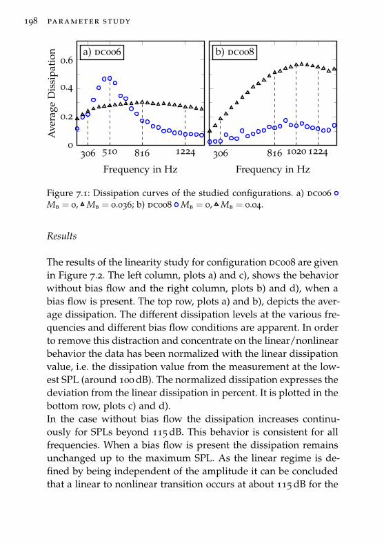
198 parameter study
306 510 816 12240
0.2
0.4
0.6a) dc006
Frequency in Hz
Ave
rage
Dis
sipa
tion
306 816 1020 1224
b) dc008
Frequency in Hz
Figure 7.1: Dissipation curves of the studied configurations. a) dc006Mb = 0, Mb = 0.036; b) dc008 Mb = 0, Mb = 0.04.
Results
The results of the linearity study for configuration dc008 are givenin Figure 7.2. The left column, plots a) and c), shows the behaviorwithout bias flow and the right column, plots b) and d), when abias flow is present. The top row, plots a) and b), depicts the aver-age dissipation. The different dissipation levels at the various fre-quencies and different bias flow conditions are apparent. In orderto remove this distraction and concentrate on the linear/nonlinearbehavior the data has been normalized with the linear dissipationvalue, i.e. the dissipation value from the measurement at the low-est SPL (around 100 dB). The normalized dissipation expresses thedeviation from the linear dissipation in percent. It is plotted in thebottom row, plots c) and d).In the case without bias flow the dissipation increases continu-ously for SPLs beyond 115 dB. This behavior is consistent for allfrequencies. When a bias flow is present the dissipation remainsunchanged up to the maximum SPL. As the linear regime is de-fined by being independent of the amplitude it can be concludedthat a linear to nonlinear transition occurs at about 115 dB for the
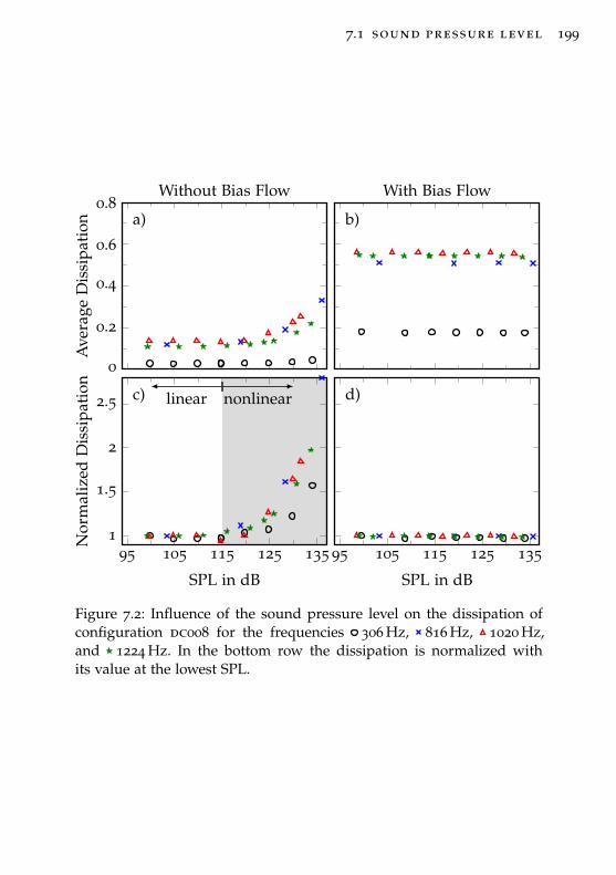
7.1 sound pressure level 199
a)
0
0.2
0.4
0.6
0.8
Ave
rage
Dis
sipa
tion
Without Bias Flow
b)
With Bias Flow
linear nonlinearc)
95 105 115 125 1351
1.5
2
2.5
SPL in dB
Nor
mal
ized
Dis
sipa
tion d)
95 105 115 125 135
SPL in dB
Figure 7.2: Influence of the sound pressure level on the dissipation ofconfiguration dc008 for the frequencies 306 Hz, 816 Hz, 1020 Hz,and 1224 Hz. In the bottom row the dissipation is normalized withits value at the lowest SPL.
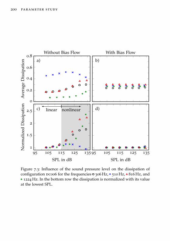
200 parameter study
a)
0
0.2
0.4
0.6
0.8
Ave
rage
Dis
sipa
tion
Without Bias Flow
b)
With Bias Flow
linear nonlinearc)
95 105 115 125 1351
1.5
2
2.5
SPL in dB
Nor
mal
ized
Dis
sipa
tion d)
95 105 115 125 135
SPL in dB
Figure 7.3: Influence of the sound pressure level on the dissipation ofconfiguration dc006 for the frequencies 306 Hz, 510 Hz, 816 Hz, and
1224 Hz. In the bottom row the dissipation is normalized with its valueat the lowest SPL.
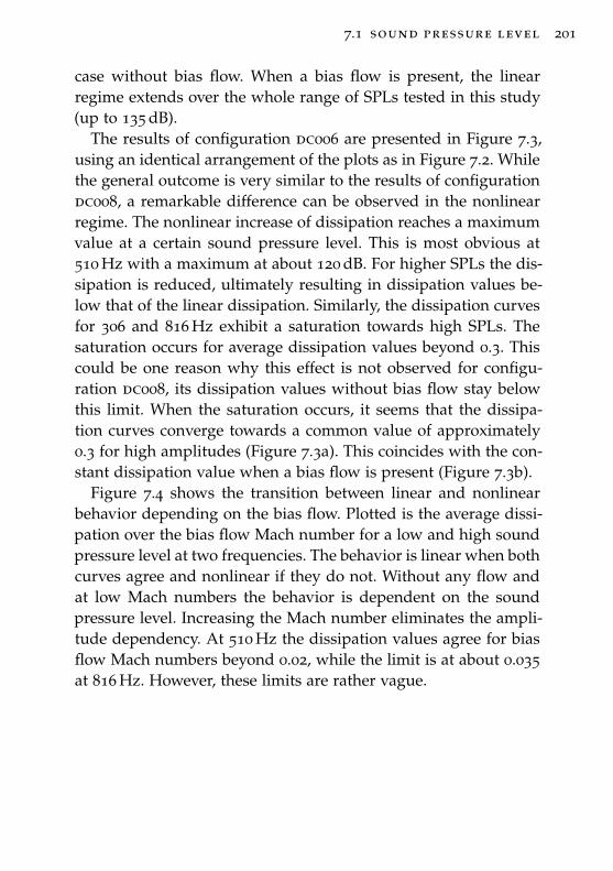
7.1 sound pressure level 201
case without bias flow. When a bias flow is present, the linearregime extends over the whole range of SPLs tested in this study(up to 135 dB).
The results of configuration dc006 are presented in Figure 7.3,using an identical arrangement of the plots as in Figure 7.2. Whilethe general outcome is very similar to the results of configurationdc008, a remarkable difference can be observed in the nonlinearregime. The nonlinear increase of dissipation reaches a maximumvalue at a certain sound pressure level. This is most obvious at510 Hz with a maximum at about 120 dB. For higher SPLs the dis-sipation is reduced, ultimately resulting in dissipation values be-low that of the linear dissipation. Similarly, the dissipation curvesfor 306 and 816 Hz exhibit a saturation towards high SPLs. Thesaturation occurs for average dissipation values beyond 0.3. Thiscould be one reason why this effect is not observed for configu-ration dc008, its dissipation values without bias flow stay belowthis limit. When the saturation occurs, it seems that the dissipa-tion curves converge towards a common value of approximately0.3 for high amplitudes (Figure 7.3a). This coincides with the con-stant dissipation value when a bias flow is present (Figure 7.3b).
Figure 7.4 shows the transition between linear and nonlinearbehavior depending on the bias flow. Plotted is the average dissi-pation over the bias flow Mach number for a low and high soundpressure level at two frequencies. The behavior is linear when bothcurves agree and nonlinear if they do not. Without any flow andat low Mach numbers the behavior is dependent on the soundpressure level. Increasing the Mach number eliminates the ampli-tude dependency. At 510 Hz the dissipation values agree for biasflow Mach numbers beyond 0.02, while the limit is at about 0.035at 816 Hz. However, these limits are rather vague.
202 parameter study
0 0.02 0.04 0.060.1
0.2
0.3
0.4
0.5a) 510 Hz
Bias Flow Mach Number
Ave
rage
Dis
sipa
tion
0 0.02 0.04 0.06
b) 816 Hz
Bias Flow Mach Number
Figure 7.4: Dissipation of configuration dc006 plotted over bias flow attwo frequencies a) 510 Hz and b) 816 Hz, comparing two sound pressurelevels 105 dB and 130 dB.
Discussion
The dependence of the orifice behavior on the sound pressurelevel seems to be fundamentally different with or without biasflow. The nonlinear behavior of orifices without bias flow has beendemonstrated and discussed in many publications [26, 58, 61, 72,105, 123, 225, 227, 228, 243, 327, 361, 441, 473, 474, 505]. The resultshere suggest a transition from linear to nonlinear behavior whenincreasing the sound pressure level beyond ≈ 115 dB. This limitseems to be independent of the frequency and the orifice diameter.These results are in agreement with previous findings. For exam-ple, the same limit was found by Tran et al. [481], studying theinfluence of the sound pressure level on the reflection coefficientof two different perforated plates. Heuwinkel et al. [199] found alimit of 110 db at 310 Hz for a cylindrical liner configuration. Leeand Kwon [287] determine a lower limit at 102 dB1.
1 A reason for this deviation could be that Lee and Kwon [287] use a randombroadband signal, where the overall SPL should be the significant quantity
7.1 sound pressure level 203
The experimental results show, that the dissipation is indepen-dent of the SPL when a bias flow is present. This behavior agreeswith the findings in [40, 199, 481]. However, this conclusion mightnot apply generally. According to Luong et al. [308], the transi-tion between linear and nonlinear regime takes place when flowreversal occurs. In that case, the oscillating acoustic velocity islarger than the steady bias flow velocity. Below this limit, Luonget al. [308] assume that the nonlinear effects are negligible2. Thislimit, based on theoretical assumption, is confirmed by the mea-surements of Rupp et al. [415, 419].
The results of the experimental study by Rupp et al. [415, 419]exhibits a similar saturation of the absorption at high amplitudesas configuration dc006 in Figure 7.3. They argue that the absoluteamount of energy that can be absorbed is fixed, so that the ab-sorption or dissipation coefficient decreases due to the increasingincident energy.
It can be concluded from the results and the discussion of theliterature, that nonlinear effects are of minor importance for biasflow liners. They only become significant when flow reversal oc-curs, that is at very high amplitudes (of course depending on thebias flow velocity). It could be argued that the pressure ampli-tudes of the instability are in fact very high. This is of course cor-rect, however, a successful liner design aims to disrupt the feed-back loop between the heat-release fluctuations and the acousticpressure fluctuations, so that an instability does not occur. Thus,the design operating point of a liner should be at much loweramplitudes.
Furthermore, flow reversal in a combustor liner leads to hotgas ingestion into the liner cavity [99, 417, 420]. This changes theabsorption characteristics of the liner and, in worst case, resultsin overheating and failure of the structure. Thus, the velocity of
(see discussion on page 31). It is not clear which definition the 102 dB arebased on.
2 Recently, Bodén and Zhou [70] showed that the nonlinear effects cannot beneglected entirely below this limit.
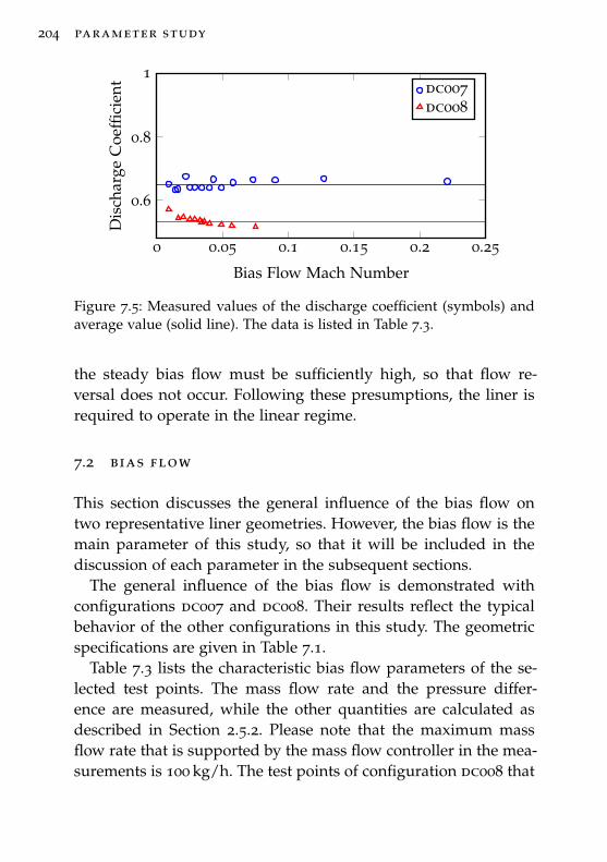
204 parameter study
0 0.05 0.1 0.15 0.2 0.25
0.6
0.8
1
Bias Flow Mach Number
Dis
char
geC
oeffi
cien
t dc007dc008
Figure 7.5: Measured values of the discharge coefficient (symbols) andaverage value (solid line). The data is listed in Table 7.3.
the steady bias flow must be sufficiently high, so that flow re-versal does not occur. Following these presumptions, the liner isrequired to operate in the linear regime.
7.2 bias flow
This section discusses the general influence of the bias flow ontwo representative liner geometries. However, the bias flow is themain parameter of this study, so that it will be included in thediscussion of each parameter in the subsequent sections.
The general influence of the bias flow is demonstrated withconfigurations dc007 and dc008. Their results reflect the typicalbehavior of the other configurations in this study. The geometricspecifications are given in Table 7.1.
Table 7.3 lists the characteristic bias flow parameters of the se-lected test points. The mass flow rate and the pressure differ-ence are measured, while the other quantities are calculated asdescribed in Section 2.5.2. Please note that the maximum massflow rate that is supported by the mass flow controller in the mea-surements is 100 kg/h. The test points of configuration dc008 that
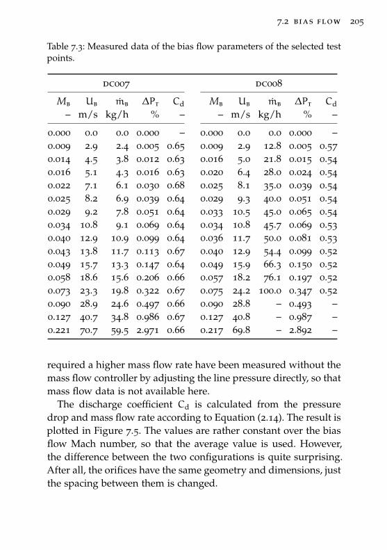
7.2 bias flow 205
Table 7.3: Measured data of the bias flow parameters of the selected testpoints.
dc007 dc008
Mb Ub mb ∆Pt Cd Mb Ub mb ∆Pt Cd
– m/s kg/h % – – m/s kg/h % –
0.000 0.0 0.0 0.000 – 0.000 0.0 0.0 0.000 –0.009 2.9 2.4 0.005 0.65 0.009 2.9 12.8 0.005 0.570.014 4.5 3.8 0.012 0.63 0.016 5.0 21.8 0.015 0.540.016 5.1 4.3 0.016 0.63 0.020 6.4 28.0 0.024 0.540.022 7.1 6.1 0.030 0.68 0.025 8.1 35.0 0.039 0.540.025 8.2 6.9 0.039 0.64 0.029 9.3 40.0 0.051 0.540.029 9.2 7.8 0.051 0.64 0.033 10.5 45.0 0.065 0.540.034 10.8 9.1 0.069 0.64 0.034 10.8 45.7 0.069 0.530.040 12.9 10.9 0.099 0.64 0.036 11.7 50.0 0.081 0.530.043 13.8 11.7 0.113 0.67 0.040 12.9 54.4 0.099 0.520.049 15.7 13.3 0.147 0.64 0.049 15.9 66.3 0.150 0.520.058 18.6 15.6 0.206 0.66 0.057 18.2 76.1 0.197 0.520.073 23.3 19.8 0.322 0.67 0.075 24.2 100.0 0.347 0.520.090 28.9 24.6 0.497 0.66 0.090 28.8 – 0.493 –0.127 40.7 34.8 0.986 0.67 0.127 40.8 – 0.987 –0.221 70.7 59.5 2.971 0.66 0.217 69.8 – 2.892 –
required a higher mass flow rate have been measured without themass flow controller by adjusting the line pressure directly, so thatmass flow data is not available here.
The discharge coefficient Cd is calculated from the pressuredrop and mass flow rate according to Equation (2.14). The result isplotted in Figure 7.5. The values are rather constant over the biasflow Mach number, so that the average value is used. However,the difference between the two configurations is quite surprising.After all, the orifices have the same geometry and dimensions, justthe spacing between them is changed.
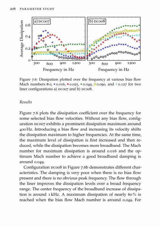
206 parameter study
a) dc007
300 600 900 12000
0.2
0.4
0.6
Frequency in Hz
Ave
rage
Dis
sipa
tion b) dc008
300 600 900 1200
Frequency in Hz
Figure 7.6: Dissipation plotted over the frequency at various bias flowMach numbers 0, 0.016, 0.025, 0.049, 0.090, and 0.127 for twoliner configurations a) dc007 and b) dc008.
Results
Figure 7.6 plots the dissipation coefficient over the frequency forsome selected bias flow velocities. Without any bias flow, config-uration dc007 exhibits a prominent dissipation maximum around400 Hz. Introducing a bias flow and increasing its velocity shiftsthe dissipation maximum to higher frequencies. At the same time,the maximum level of dissipation is first increased and then re-duced, while the dissipation becomes more broadband. The Machnumber for maximum dissipation is around 0.016 and the op-timum Mach number to achieve a good broadband damping isaround 0.049.
Configuration dc008 in Figure 7.6b demonstrates different char-acteristics. The damping is very poor when there is no bias flowpresent and there is no obvious peak frequency. The flow throughthe liner improves the dissipation levels over a broad frequencyrange. The center frequency of the broadband increase of dissipa-tion is around 1 kHz. A maximum dissipation of nearly 60 % isreached when the bias flow Mach number is around 0.049. For
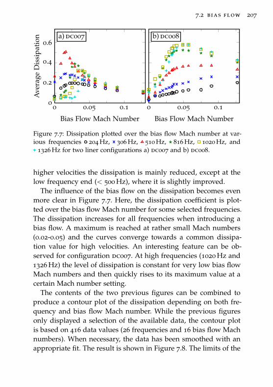
7.2 bias flow 207
a) dc007
0 0.05 0.10
0.2
0.4
0.6
Bias Flow Mach Number
Ave
rage
Dis
sipa
tion b) dc008
0 0.05 0.1
Bias Flow Mach Number
Figure 7.7: Dissipation plotted over the bias flow Mach number at var-ious frequencies 204 Hz, 306 Hz, 510 Hz, 816 Hz, 1020 Hz, and
1326 Hz for two liner configurations a) dc007 and b) dc008.
higher velocities the dissipation is mainly reduced, except at thelow frequency end (< 500 Hz), where it is slightly improved.
The influence of the bias flow on the dissipation becomes evenmore clear in Figure 7.7. Here, the dissipation coefficient is plot-ted over the bias flow Mach number for some selected frequencies.The dissipation increases for all frequencies when introducing abias flow. A maximum is reached at rather small Mach numbers(0.02-0.05) and the curves converge towards a common dissipa-tion value for high velocities. An interesting feature can be ob-served for configuration dc007. At high frequencies (1020 Hz and1326 Hz) the level of dissipation is constant for very low bias flowMach numbers and then quickly rises to its maximum value at acertain Mach number setting.
The contents of the two previous figures can be combined toproduce a contour plot of the dissipation depending on both fre-quency and bias flow Mach number. While the previous figuresonly displayed a selection of the available data, the contour plotis based on 416 data values (26 frequencies and 16 bias flow Machnumbers). When necessary, the data has been smoothed with anappropriate fit. The result is shown in Figure 7.8. The limits of the
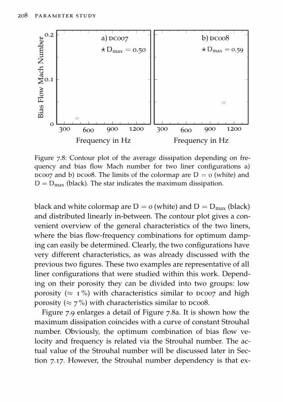
208 parameter study
a) dc007
300 600 900 12000
0.1
0.2
Frequency in Hz
Bias
Flow
Mac
hN
umbe
rDmax = 0.50
b) dc008
300 600 900 1200
Frequency in Hz
Dmax = 0.59
Figure 7.8: Contour plot of the average dissipation depending on fre-quency and bias flow Mach number for two liner configurations a)dc007 and b) dc008. The limits of the colormap are D = 0 (white) andD = Dmax (black). The star indicates the maximum dissipation.
black and white colormap areD = 0 (white) andD = Dmax (black)and distributed linearly in-between. The contour plot gives a con-venient overview of the general characteristics of the two liners,where the bias flow-frequency combinations for optimum damp-ing can easily be determined. Clearly, the two configurations havevery different characteristics, as was already discussed with theprevious two figures. These two examples are representative of allliner configurations that were studied within this work. Depend-ing on their porosity they can be divided into two groups: lowporosity (≈ 1 %) with characteristics similar to dc007 and highporosity (≈ 7 %) with characteristics similar to dc008.
Figure 7.9 enlarges a detail of Figure 7.8a. It is shown how themaximum dissipation coincides with a curve of constant Strouhalnumber. Obviously, the optimum combination of bias flow ve-locity and frequency is related via the Strouhal number. The ac-tual value of the Strouhal number will be discussed later in Sec-tion 7.17. However, the Strouhal number dependency is that ex-
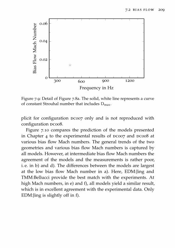
7.2 bias flow 209
300 600 900 12000
0.02
0.04
0.06
Frequency in Hz
Bias
Flow
Mac
hN
umbe
r
Figure 7.9: Detail of Figure 7.8a. The solid, white line represents a curveof constant Strouhal number that includes Dmax.
plicit for configuration dc007 only and is not reproduced withconfiguration dc008.
Figure 7.10 compares the prediction of the models presentedin Chapter 4 to the experimental results of dc007 and dc008 atvarious bias flow Mach numbers. The general trends of the twogeometries and various bias flow Mach numbers is captured byall models. However, at intermediate bias flow Mach numbers theagreement of the models and the measurements is rather poor,i. e. in b) and d). The differences between the models are largestat the low bias flow Mach number in a). Here, EDM:Jing andTMM:Bellucci provide the best match with the experiments. Athigh Mach numbers, in e) and f), all models yield a similar result,which is in excellent agreement with the experimental data. OnlyEDM:Jing is slightly off in f).
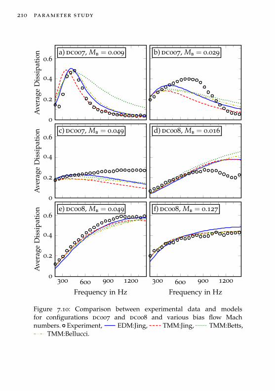
210 parameter study
a) dc007, Mb = 0.009
0
0.2
0.4
0.6
Ave
rage
Dis
sipa
tion b) dc007, Mb = 0.029
c) dc007, Mb = 0.049
0
0.2
0.4
0.6
Ave
rage
Dis
sipa
tion d) dc008, Mb = 0.016
e) dc008, Mb = 0.049
300 600 900 12000
0.2
0.4
0.6
Frequency in Hz
Ave
rage
Dis
sipa
tion f) dc008, Mb = 0.127
300 600 900 1200
Frequency in Hz
Figure 7.10: Comparison between experimental data and modelsfor configurations dc007 and dc008 and various bias flow Machnumbers. Experiment, EDM:Jing, TMM:Jing, TMM:Betts,
TMM:Bellucci.
7.2 bias flow 211
Discussion
The results show, that a bias flow does improve the absorptionof a perforated liner compared to the same configuration withoutbias flow. These findings comply with the results reported in [41,142, 161, 198, 219, 241], for example.
There exists an optimum bias flow, where the absorption is max-imum. Eldredge and Dowling [142] find the optimum Mach num-ber to be 0.015 for the liner geometry specified in Table 4.1. Theyderive an optimum ratio of bias flow Mach number to porosity. Inorder to achieve maximum absorption the liner should obey(
Mb
σ
)opt
=PL/A
2√
2. (7.1)
Applying the equation above to configurations dc007 and dc008,where for both PL/A = 1.46, the optimum bias flow Mach num-bers should be 0.0052 and 0.035, respectively. This is in contrastto the optimum bias flow Mach numbers revealed by the exper-iments: 0.016-0.049 for dc007 and 0.049 for dc008. While the re-sults for dc008 are in the same range, the estimation for dc007 isvery far off. A similar outcome was reported by Macquisten et al.[310]. They found Equation (7.1) to underestimate the optimumbias flow Mach number, especially when the number of orificerows is low.
The two liner configurations presented here demonstrate verydifferent characteristics. Without bias flow, configuration dc007exhibits a typical resonance damping behavior3. The bias flowmodifies this resonance effect until a sufficiently high bias flowvelocity is reached, beyond which the bias flow effect dominates.On the other hand, no obvious resonance effect can be observed
3 At the location of the perforation, the incident wave from the duct and thereflected wave from the cavity are 180° out of phase, so that they cancel eachother out.
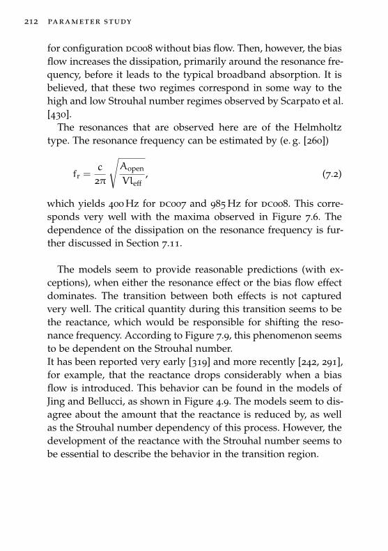
212 parameter study
for configuration dc008 without bias flow. Then, however, the biasflow increases the dissipation, primarily around the resonance fre-quency, before it leads to the typical broadband absorption. It isbelieved, that these two regimes correspond in some way to thehigh and low Strouhal number regimes observed by Scarpato et al.[430].
The resonances that are observed here are of the Helmholtztype. The resonance frequency can be estimated by (e. g. [260])
fr =c
2π
√Aopen
Vleff, (7.2)
which yields 400 Hz for dc007 and 985 Hz for dc008. This corre-sponds very well with the maxima observed in Figure 7.6. Thedependence of the dissipation on the resonance frequency is fur-ther discussed in Section 7.11.
The models seem to provide reasonable predictions (with ex-ceptions), when either the resonance effect or the bias flow effectdominates. The transition between both effects is not capturedvery well. The critical quantity during this transition seems to bethe reactance, which would be responsible for shifting the reso-nance frequency. According to Figure 7.9, this phenomenon seemsto be dependent on the Strouhal number.It has been reported very early [319] and more recently [242, 291],for example, that the reactance drops considerably when a biasflow is introduced. This behavior can be found in the models ofJing and Bellucci, as shown in Figure 4.9. The models seem to dis-agree about the amount that the reactance is reduced by, as wellas the Strouhal number dependency of this process. However, thedevelopment of the reactance with the Strouhal number seems tobe essential to describe the behavior in the transition region.
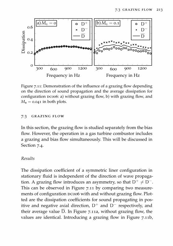
7.3 grazing flow 213
a) Mg = 0
300 600 900 12000
0.2
0.4
0.6
Frequency in Hz
Dis
sipa
tion
D+
D−
D
b) Mg = 0.1
300 600 900 1200
Frequency in Hz
D+
D−
D
Figure 7.11: Demonstration of the influence of a grazing flow dependingon the direction of sound propagation and the average dissipation forconfiguration dc006: a) without grazing flow, b) with grazing flow, andMb = 0.041 in both plots.
7.3 grazing flow
In this section, the grazing flow is studied separately from the biasflow. However, the operation in a gas turbine combustor includesa grazing and bias flow simultaneously. This will be discussed inSection 7.4.
Results
The dissipation coefficient of a symmetric liner configuration instationary fluid is independent of the direction of wave propaga-tion. A grazing flow introduces an asymmetry, so that D+ 6= D−.This can be observed in Figure 7.11 by comparing two measure-ments of configuration dc006 with and without grazing flow. Plot-ted are the dissipation coefficients for sound propagating in pos-itive and negative axial direction, D+ and D− respectively, andtheir average value D. In Figure 7.11a, without grazing flow, thevalues are identical. Introducing a grazing flow in Figure 7.11b,
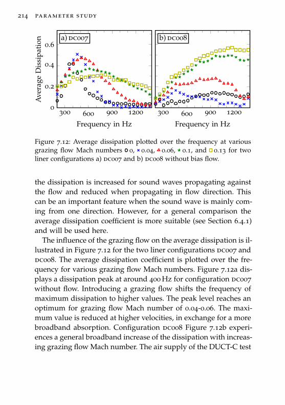
214 parameter study
a) dc007
300 600 900 12000
0.2
0.4
0.6
Frequency in Hz
Ave
rage
Dis
sipa
tion b) dc008
300 600 900 1200
Frequency in Hz
Figure 7.12: Average dissipation plotted over the frequency at variousgrazing flow Mach numbers 0, 0.04, 0.06, 0.1, and 0.13 for twoliner configurations a) dc007 and b) dc008 without bias flow.
the dissipation is increased for sound waves propagating againstthe flow and reduced when propagating in flow direction. Thiscan be an important feature when the sound wave is mainly com-ing from one direction. However, for a general comparison theaverage dissipation coefficient is more suitable (see Section 6.4.1)and will be used here.
The influence of the grazing flow on the average dissipation is il-lustrated in Figure 7.12 for the two liner configurations dc007 anddc008. The average dissipation coefficient is plotted over the fre-quency for various grazing flow Mach numbers. Figure 7.12a dis-plays a dissipation peak at around 400 Hz for configuration dc007without flow. Introducing a grazing flow shifts the frequency ofmaximum dissipation to higher values. The peak level reaches anoptimum for grazing flow Mach number of 0.04-0.06. The maxi-mum value is reduced at higher velocities, in exchange for a morebroadband absorption. Configuration dc008 Figure 7.12b experi-ences a general broadband increase of the dissipation with increas-ing grazing flow Mach number. The air supply of the DUCT-C test
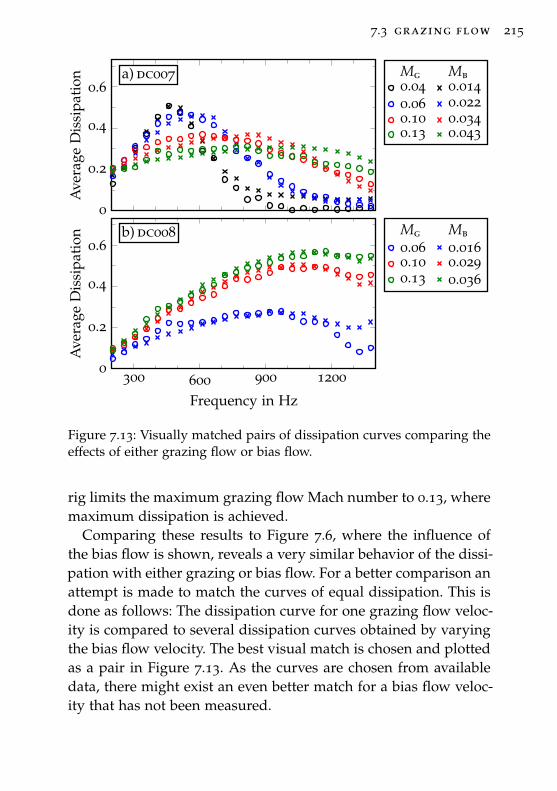
7.3 grazing flow 215
a) dc007
0
0.2
0.4
0.6A
vera
geD
issi
pati
onMg Mb0.04 0.0140.06 0.0220.10 0.0340.13 0.043
b) dc008
300 600 900 12000
0.2
0.4
0.6
Frequency in Hz
Ave
rage
Dis
sipa
tion
Mg Mb0.06 0.0160.10 0.0290.13 0.036
Figure 7.13: Visually matched pairs of dissipation curves comparing theeffects of either grazing flow or bias flow.
rig limits the maximum grazing flow Mach number to 0.13, wheremaximum dissipation is achieved.
Comparing these results to Figure 7.6, where the influence ofthe bias flow is shown, reveals a very similar behavior of the dissi-pation with either grazing or bias flow. For a better comparison anattempt is made to match the curves of equal dissipation. This isdone as follows: The dissipation curve for one grazing flow veloc-ity is compared to several dissipation curves obtained by varyingthe bias flow velocity. The best visual match is chosen and plottedas a pair in Figure 7.13. As the curves are chosen from availabledata, there might exist an even better match for a bias flow veloc-ity that has not been measured.
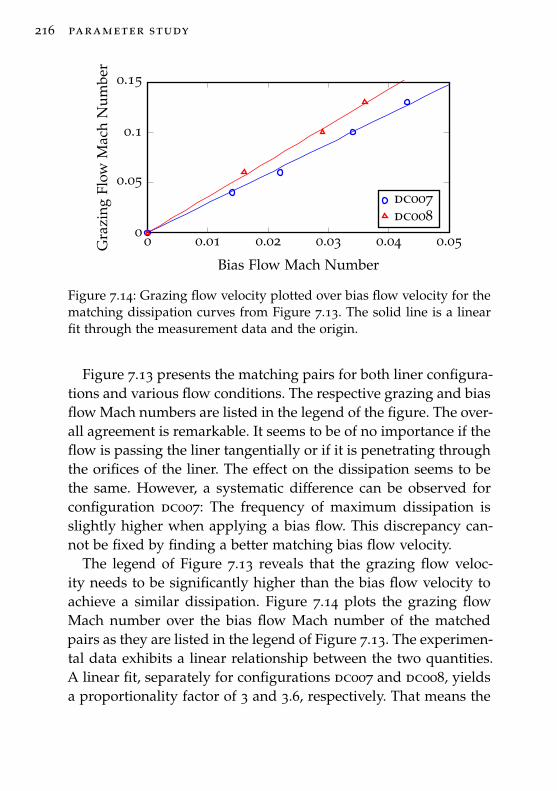
216 parameter study
0 0.01 0.02 0.03 0.04 0.050
0.05
0.1
0.15
Bias Flow Mach Number
Gra
zing
Flow
Mac
hN
umbe
r
dc007dc008
Figure 7.14: Grazing flow velocity plotted over bias flow velocity for thematching dissipation curves from Figure 7.13. The solid line is a linearfit through the measurement data and the origin.
Figure 7.13 presents the matching pairs for both liner configura-tions and various flow conditions. The respective grazing and biasflow Mach numbers are listed in the legend of the figure. The over-all agreement is remarkable. It seems to be of no importance if theflow is passing the liner tangentially or if it is penetrating throughthe orifices of the liner. The effect on the dissipation seems to bethe same. However, a systematic difference can be observed forconfiguration dc007: The frequency of maximum dissipation isslightly higher when applying a bias flow. This discrepancy can-not be fixed by finding a better matching bias flow velocity.
The legend of Figure 7.13 reveals that the grazing flow veloc-ity needs to be significantly higher than the bias flow velocity toachieve a similar dissipation. Figure 7.14 plots the grazing flowMach number over the bias flow Mach number of the matchedpairs as they are listed in the legend of Figure 7.13. The experimen-tal data exhibits a linear relationship between the two quantities.A linear fit, separately for configurations dc007 and dc008, yieldsa proportionality factor of 3 and 3.6, respectively. That means the
7.3 grazing flow 217
velocity of the grazing flow needs to be about 3.3 times higher asthe bias flow velocity to achieve a similar absorption. It remainsunclear if the deviation between the two configurations is a physi-cal reality or if it is a result of the quite vague method of matchingthe dissipation curves, so that the proportionality factor shouldonly be regarded as rough estimate.
Discussion
Evaluating D+ and D− separately reveals, that the absorption isreduced for sound traveling in grazing flow direction while it isincreased by a similar amount when propagating in the oppositedirection. This effect is discussed in [226, 264, 274, 321, 322, 324,329, 349, 374, 467] and the difference between D+ and D− is ac-credited with two phenomena:
1 . The velocity gradient within the flow boundary layer refractsthe direction of propagation of the sound wave. While the wavenormal without flow is assumed to be parallel to the wall (ne-glecting any acoustic boundary layer), it is refracted into the linerwhen propagating downstream and away from the liner whenpropagating upstream. This would result in an increased absorp-tion for sound waves propagating in flow direction and a reduc-tion against flow. This phenomenon is pronounced at higher fre-quencies and Tack and Lambert [467] suggest to neglect it whenkδ 6 0.1, where δ is the thickness of the flow boundary layer.
2 . The convective effect of the flow modifies the phase velocityof the wave by a factor 1+Mg in flow direction and 1−Mg against,increasing and reducing the wave length respectively. Thus the ab-sorption per wave length remains constant when a grazing flowis present, while the absorption due to a liner of fixed length is re-duced for waves traveling downstream and increased against flowdirection [321].
218 parameter study
Both phenomena have a converse effect on increasing and reduc-ing the dissipation. It can be observed in Figure 7.11 that the sec-ond phenomena dominates here.
The effect of the grazing flow on the average dissipation iscorresponding to the bias flow effect. In fact, similar results areachieved when Mg ≈ 3.3 Mb. This similarity between the influenceof grazing and bias flow on the dissipation was also observed byFeder and Dean [158]. They compared the grazing flow velocityto the bias flow velocity producing the same change of resistance.Their measurements include six perforations with varying poros-ity (10-35 %) and two grazing flow velocities (90 and 150 m/s). Theratio of grazing to bias flow velocity is virtually independent ofthe porosity, but different values are obtained for the two graz-ing flow velocities. They arrive at ratios of approximately 8 and5 for the low and high grazing flow velocity, respectively. Theircalculation of the bias flow velocity neglects the orifice dischargecoefficient. Applying a general discharge coefficient of 0.61 yieldsratios of grazing to bias flow velocities of about 5 and 3, which isin good agreement with the values obtained here.The impedance model of Bauer contains a term for the resistancedue to the grazing flow and a second term for the resistance dueto the bias flow (see Section 4.6). Both terms are identical, exceptfor a factor of 3.8 between them. This corresponds very well to theexperimental finding discussed above.
Judging by the similarity of the grazing flow and bias flow ef-fects, the absorption mechanism seems to be the same, i. e. theconversion of acoustic energy into shedding vorticity. Feder andDean suggest the following explanation of the grazing flow phe-nomenon [158, p. 22]: “The reason for this similarity is believedto be due to boundary layer fluctuations, induced by the grazingflow velocities, causing airflows through the specimens. The fre-quency of these fluctuations is believed to be low enough so that
7.4 simultaneous grazing & bias flow 219
the resulting through flows affect the acoustic characteristics ofthe specimens in a manner similar to steady through flows.”
The results above demonstrate a throughout positive effect ofthe grazing flow on the acoustic performance of a perforated liner.However, it has been reported, that at certain combinations ofgrazing flow velocity and liner geometry, depending on the ori-fice Strouhal number, sound might be generated rather than ab-sorbed (see [23, 75, 216, 321, 377], for example). This effect oc-curred during the measurements here for configuration dc008 atMg = 0.05 and produced a dominant tone at about 1300 Hz. How-ever, slightly changing the grazing flow velocity or introducing abias flow suppressed the phenomena.
7.4 simultaneous grazing & bias flow
The effects of grazing flow and bias flow are mostly studied sepa-rately, as was done in the two previous sections. However, whenboth are present simultaneously, the result might be influenced bythe interaction of the two.
Results
Figure 7.15 shows dissipation curves at two bias flow velocitiesfor varying grazing flow Mach number. In Figure 7.15a, at the lowbias flow Mach number, the dissipation increases with the super-position of the grazing flow. At the faster bias flow, in Figure 7.15b,the result is unimpressed by the grazing flow.
The superposition of grazing and bias flow does not improvethe dissipation beyond what can be achieved by applying eitherone alone. There seems to be an upper limit of dissipation whichcannot be surpassed by the combination of grazing and bias flow.So, if any of the two velocities is already at an optimum (for max-imum dissipation), then the other imposes only a minor or noinfluence on the result.
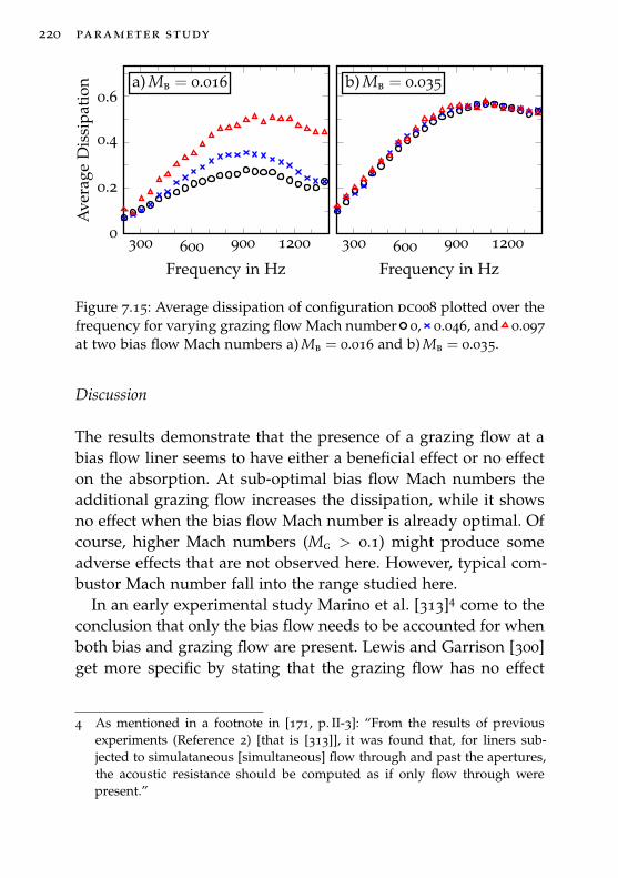
220 parameter study
a) Mb = 0.016
300 600 900 12000
0.2
0.4
0.6
Frequency in Hz
Ave
rage
Dis
sipa
tion b) Mb = 0.035
300 600 900 1200
Frequency in Hz
Figure 7.15: Average dissipation of configuration dc008 plotted over thefrequency for varying grazing flow Mach number 0, 0.046, and 0.097at two bias flow Mach numbers a) Mb = 0.016 and b) Mb = 0.035.
Discussion
The results demonstrate that the presence of a grazing flow at abias flow liner seems to have either a beneficial effect or no effecton the absorption. At sub-optimal bias flow Mach numbers theadditional grazing flow increases the dissipation, while it showsno effect when the bias flow Mach number is already optimal. Ofcourse, higher Mach numbers (Mg > 0.1) might produce someadverse effects that are not observed here. However, typical com-bustor Mach number fall into the range studied here.
In an early experimental study Marino et al. [313]4 come to theconclusion that only the bias flow needs to be accounted for whenboth bias and grazing flow are present. Lewis and Garrison [300]get more specific by stating that the grazing flow has no effect
4 As mentioned in a footnote in [171, p. II-3]: “From the results of previousexperiments (Reference 2) [that is [313]], it was found that, for liners sub-jected to simulataneous [simultaneous] flow through and past the apertures,the acoustic resistance should be computed as if only flow through werepresent.”
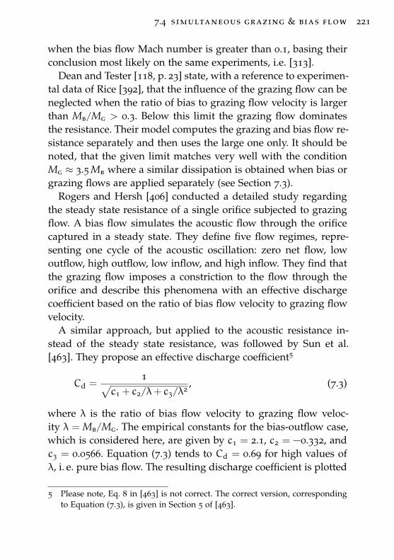
7.4 simultaneous grazing & bias flow 221
when the bias flow Mach number is greater than 0.1, basing theirconclusion most likely on the same experiments, i.e. [313].
Dean and Tester [118, p. 23] state, with a reference to experimen-tal data of Rice [392], that the influence of the grazing flow can beneglected when the ratio of bias to grazing flow velocity is largerthan Mb/Mg > 0.3. Below this limit the grazing flow dominatesthe resistance. Their model computes the grazing and bias flow re-sistance separately and then uses the large one only. It should benoted, that the given limit matches very well with the conditionMg ≈ 3.5 Mb where a similar dissipation is obtained when bias orgrazing flows are applied separately (see Section 7.3).
Rogers and Hersh [406] conducted a detailed study regardingthe steady state resistance of a single orifice subjected to grazingflow. A bias flow simulates the acoustic flow through the orificecaptured in a steady state. They define five flow regimes, repre-senting one cycle of the acoustic oscillation: zero net flow, lowoutflow, high outflow, low inflow, and high inflow. They find thatthe grazing flow imposes a constriction to the flow through theorifice and describe this phenomena with an effective dischargecoefficient based on the ratio of bias flow velocity to grazing flowvelocity.
A similar approach, but applied to the acoustic resistance in-stead of the steady state resistance, was followed by Sun et al.[463]. They propose an effective discharge coefficient5
Cd =1√
c1 + c2/λ+ c3/λ2, (7.3)
where λ is the ratio of bias flow velocity to grazing flow veloc-ity λ = Mb/Mg. The empirical constants for the bias-outflow case,which is considered here, are given by c1 = 2.1, c2 = −0.332, andc3 = 0.0566. Equation (7.3) tends to Cd = 0.69 for high values ofλ, i. e. pure bias flow. The resulting discharge coefficient is plotted
5 Please note, Eq. 8 in [463] is not correct. The correct version, correspondingto Equation (7.3), is given in Section 5 of [463].
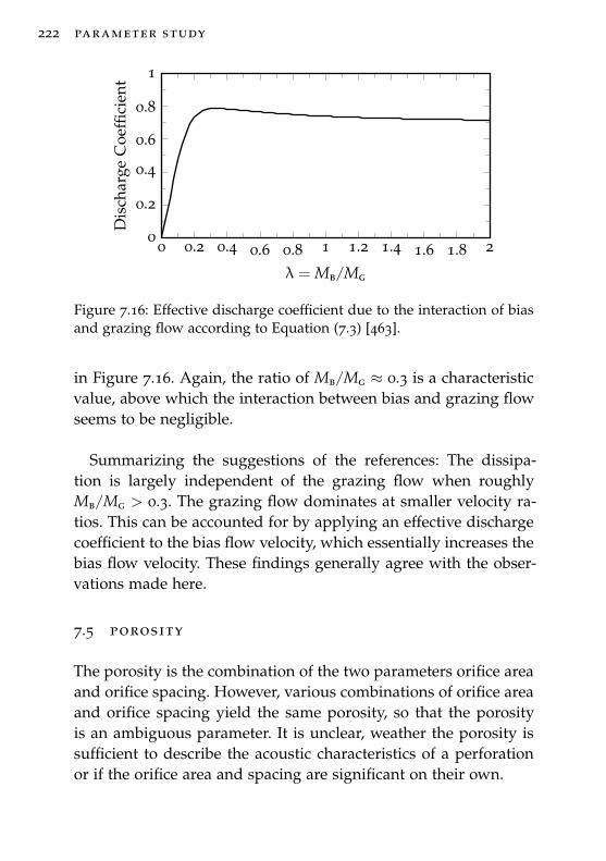
222 parameter study
0 0.2 0.4 0.6 0.8 1 1.2 1.4 1.6 1.8 20
0.2
0.4
0.6
0.8
1
λ = Mb/Mg
Dis
char
geC
oeffi
cien
t
Figure 7.16: Effective discharge coefficient due to the interaction of biasand grazing flow according to Equation (7.3) [463].
in Figure 7.16. Again, the ratio of Mb/Mg ≈ 0.3 is a characteristicvalue, above which the interaction between bias and grazing flowseems to be negligible.
Summarizing the suggestions of the references: The dissipa-tion is largely independent of the grazing flow when roughlyMb/Mg > 0.3. The grazing flow dominates at smaller velocity ra-tios. This can be accounted for by applying an effective dischargecoefficient to the bias flow velocity, which essentially increases thebias flow velocity. These findings generally agree with the obser-vations made here.
7.5 porosity
The porosity is the combination of the two parameters orifice areaand orifice spacing. However, various combinations of orifice areaand orifice spacing yield the same porosity, so that the porosityis an ambiguous parameter. It is unclear, weather the porosity issufficient to describe the acoustic characteristics of a perforationor if the orifice area and spacing are significant on their own.
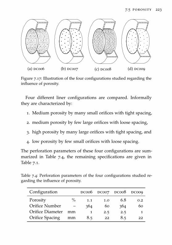
7.5 porosity 223
(a) dc006 (b) dc007 (c) dc008 (d) dc009
Figure 7.17: Illustration of the four configurations studied regarding theinfluence of porosity.
Four different liner configurations are compared. Informallythey are characterized by:
1. Medium porosity by many small orifices with tight spacing,
2. medium porosity by few large orifices with loose spacing,
3. high porosity by many large orifices with tight spacing, and
4. low porosity by few small orifices with loose spacing.
The perforation parameters of these four configurations are sum-marized in Table 7.4, the remaining specifications are given inTable 7.1.
Table 7.4: Perforation parameters of the four configurations studied re-garding the influence of porosity.
Configuration dc006 dc007 dc008 dc009
Porosity % 1.1 1.0 6.8 0.2Orifice Number – 364 60 364 60Orifice Diameter mm 1 2.5 2.5 1Orifice Spacing mm 8.5 22 8.5 22
224 parameter study
Results
Figure 7.18 compares the four configurations at various bias flowMach numbers. Without flow and at low Mach numbers the re-sults of the four configurations are very different. With increasingbias flow Mach number, the curves of equal porosity align moreand more, so that they become identical for Mb > 0.049. This is re-markable, as apart from the porosity the geometric specificationsare quite different. The porosity is clearly the significant parame-ter at higher bias flow Mach numbers, overruling the orifice area,the orifice spacing, and the number of orifices.
At the same time it becomes obvious, that higher porositiesyield an increased absorption. Again, this trend is only revealedat higher bias flow Mach numbers.
Figure 7.19 reproduces Figure 7.18d and includes the modelpredictions for all four porosities. While the details of each modelvanish in the multitude of lines, it can be observed at a glance thatall models capture the general influence of the porosity success-fully.
Matching the porosity of two liners yields nearly identical re-sults in the experiments. The models, however, show a greatervariation when comparing dc006 and dc007. In order to allowa more detailed comparison, these two configurations are plot-ted separately in Figure 7.20. For convenience, the differences be-tween the two configurations are indicated by filling the area be-tween the respective curves with the associated color. It is obviousthat the models do not depend on the porosity alone, but that theorifice diameter, the orifice spacing, or the number of orifices hasan impact on the prediction. This is in contrast to the experimentalresults. However, the general agreement between the experimentand the models of these particular configurations is satisfactoryat best. Especially, the broadband nature of the damping is notcaptured correctly.
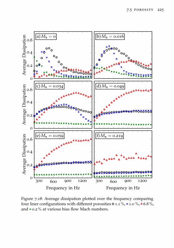
7.5 porosity 225
a) Mb = 0
0
0.2
0.4
0.6
Ave
rage
Dis
sipa
tion b) Mb = 0.016
c) Mb = 0.034
0
0.2
0.4
0.6
Ave
rage
Dis
sipa
tion d) Mb = 0.049
e) Mb = 0.059
300 600 900 12000
0.2
0.4
0.6
Frequency in Hz
Ave
rage
Dis
sipa
tion f) Mb = 0.219
300 600 900 1200
Frequency in Hz
Figure 7.18: Average dissipation plotted over the frequency comparingfour liner configurations with different porosities 1.1 %, 1.0 %, 6.8 %,and 0.2 % at various bias flow Mach numbers.
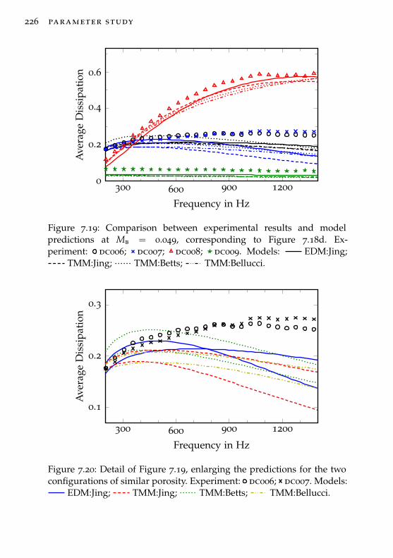
226 parameter study
300 600 900 12000
0.2
0.4
0.6
Frequency in Hz
Ave
rage
Dis
sipa
tion
Figure 7.19: Comparison between experimental results and modelpredictions at Mb = 0.049, corresponding to Figure 7.18d. Ex-periment: dc006; dc007; dc008; dc009. Models: EDM:Jing;
TMM:Jing; TMM:Betts; TMM:Bellucci.
300 600 900 1200
0.1
0.2
0.3
Frequency in Hz
Ave
rage
Dis
sipa
tion
Figure 7.20: Detail of Figure 7.19, enlarging the predictions for the twoconfigurations of similar porosity. Experiment: dc006; dc007. Models:
EDM:Jing; TMM:Jing; TMM:Betts; TMM:Bellucci.
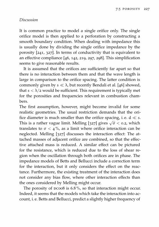
7.5 porosity 227
Discussion
It is common practice to model a single orifice only. The singleorifice model is then applied to a perforation by constructing asmooth boundary condition. When dealing with impedance thisis usually done by dividing the single orifice impedance by theporosity [241, 327]. In terms of conductivity that is equivalent toan effective compliance [46, 142, 219, 297, 298]. This simplificationseems to give reasonable results.
It is assumed that the orifices are sufficiently far apart so thatthere is no interaction between them and that the wave length islarge in comparison to the orifice spacing. The latter condition iscommonly given by s� λ, but recently Bendali et al. [46] showed,that s < λ/2 would be sufficient. This requirement is typically metfor the porosities and frequencies relevant in combustion cham-bers.The first assumption, however, might become invalid for somerealistic geometries. The usual restriction demands that the ori-fice diameter is much smaller than the orifice spacing, i. e. d � s.This is a rather vague limit. Melling [327] gives
√σ < 0.2, which
translates to σ < 4 %, as a limit where orifice interaction can beneglected. Melling [327] discusses the interaction effect: The at-tached masses of adjacent orifice are combined, so that the effec-tive attached mass is reduced. A similar effect can be picturedfor the resistance, which is reduced due to the loss of shear re-gion when the oscillation through both orifices are in phase. Theimpedance models of Betts and Bellucci include a correction termfor the interaction, but it only considers the effect on the reac-tance. Furthermore, the existing treatment of the interaction doesnot consider any bias flow, where other interaction effects thanthe ones considered by Melling might occur.
The porosity of dc008 is 6.8 %, so that interaction might occur.Indeed, it seems that the models which take the interaction into ac-count, i. e. Betts and Bellucci, predict a slightly higher frequency of
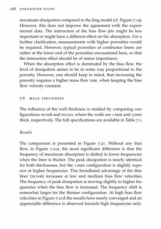
228 parameter study
maximum dissipation compared to the Jing model (cf. Figure 7.19).However, this does not improve the agreement with the experi-mental data. The interaction of the bias flow jets might be lessimportant or might have a different effect on the absorption. For afurther clarification, measurements with higher porosities wouldbe required. However, typical porosities of combustor liners arerather at the lower end of the porosities encountered here, so thatthe interaction effect should be of minor importance.
When the absorption effect is dominated by the bias flow, thelevel of dissipation seems to be in some way proportional to theporosity. However, one should keep in mind, that increasing theporosity requires a higher mass flow rate, when keeping the biasflow velocity constant.
7.6 wall thickness
The influence of the wall thickness is studied by comparing con-figurations dc006 and dc010, where the walls are 1 mm and 3 mmthick, respectively. The full specifications are available in Table 7.1.
Results
The comparison is presented in Figure 7.21. Without any biasflow, in Figure 7.21a, the most significant difference is that thefrequency of maximum absorption is shifted to lower frequencieswhen the liner is thicker. The peak dissipation is nearly identicalfor both thicknesses, but the 1 mm configuration is slightly supe-rior at higher frequencies. This broadband advantage of the thinliner (dc006) increases at low and medium bias flow velocities.The frequency of peak dissipation is moving slightly to higher fre-quencies when the bias flow is increased. The frequency shift issomewhat larger for the thinner configuration. At high bias flowvelocities in Figure 7.21d the results have nearly converged and anappreciable difference is observed towards high frequencies only.
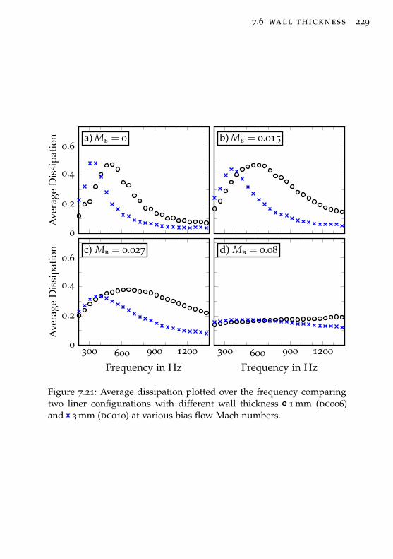
7.6 wall thickness 229
a) Mb = 0
0
0.2
0.4
0.6
Ave
rage
Dis
sipa
tion b) Mb = 0.015
c) Mb = 0.027
300 600 900 12000
0.2
0.4
0.6
Frequency in Hz
Ave
rage
Dis
sipa
tion d) Mb = 0.08
300 600 900 1200
Frequency in Hz
Figure 7.21: Average dissipation plotted over the frequency comparingtwo liner configurations with different wall thickness 1 mm (dc006)and 3 mm (dc010) at various bias flow Mach numbers.
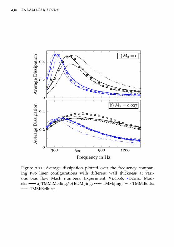
230 parameter study
a) Mb = 0
0
0.2
0.4
Ave
rage
Dis
sipa
tion
b) Mb = 0.027
300 600 900 12000
0.2
0.4
Frequency in Hz
Ave
rage
Dis
sipa
tion
Figure 7.22: Average dissipation plotted over the frequency compar-ing two liner configurations with different wall thickness at vari-ous bias flow Mach numbers. Experiment: dc006; dc010. Mod-els: a) TMM:Melling/b) EDM:Jing; TMM:Jing; TMM:Betts;
TMM:Bellucci.
7.7 orifice cross-section shape 231
Without bias flow in Figure 7.22a the best agreement with ex-perimental data is achieved by TMM:Melling. The other models,TMM:Betts and TMM:Bellucci, reproduce the general trend whenchanging the thickness, but exhibit less optimal agreement withthe measurements. However, the agreement is better for dc010.The predictions follow the trend also at Mb = 0.027. Again, theagreement is better for the thicker configuration, while all modelsunderpredict the dissipation for dc006.
Discussion
The wall thickness is a prominent parameter in any of the ori-fice models presented in Chapter 4. Without flow, the thicknesseffect is well understood. A longer orifice increases the mass iner-tance and the viscous losses. The main effects on the dissipationare the decrease of the peak frequency and the increase of theQ factor, cf. [41, 241]. Both effects are reproduced in the exper-imental data presented here and predicted rather accurately byTMM:Melling. Both, TMM:Betts and TMM:Bellucci, yield a betteragreement with the experiments for the 3 mm wall thickness. Bothmodels use an approximation of Equation (4.12), which seems tobe suited better at this larger thickness.
When a bias flow is present the absorption characteristics of thethin wall are clearly superior with a higher peak absorption andcovering a wider frequency range. This is in agreement with theexperimental results of Jing and Sun [241] and Bellucci et al. [41].
7.7 orifice cross-section shape
The standard orifices in this study have a circular cross-section.Now, the dissipation characteristics of a circular orifice is com-pared to a cross-shaped orifice with equal open area. The geom-etry of the cross-shaped orifice is illustrated in Figure 2.5g withthe dimensions l1 = 1 mm and l2 = 1 mm. The characteristic spec-
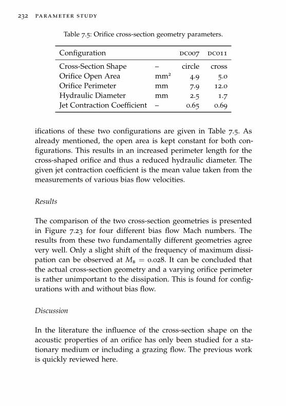
232 parameter study
Table 7.5: Orifice cross-section geometry parameters.
Configuration dc007 dc011
Cross-Section Shape – circle crossOrifice Open Area mm2 4.9 5.0Orifice Perimeter mm 7.9 12.0Hydraulic Diameter mm 2.5 1.7Jet Contraction Coefficient – 0.65 0.69
ifications of these two configurations are given in Table 7.5. Asalready mentioned, the open area is kept constant for both con-figurations. This results in an increased perimeter length for thecross-shaped orifice and thus a reduced hydraulic diameter. Thegiven jet contraction coefficient is the mean value taken from themeasurements of various bias flow velocities.
Results
The comparison of the two cross-section geometries is presentedin Figure 7.23 for four different bias flow Mach numbers. Theresults from these two fundamentally different geometries agreevery well. Only a slight shift of the frequency of maximum dissi-pation can be observed at Mb = 0.028. It can be concluded thatthe actual cross-section geometry and a varying orifice perimeteris rather unimportant to the dissipation. This is found for config-urations with and without bias flow.
Discussion
In the literature the influence of the cross-section shape on theacoustic properties of an orifice has only been studied for a sta-tionary medium or including a grazing flow. The previous workis quickly reviewed here.
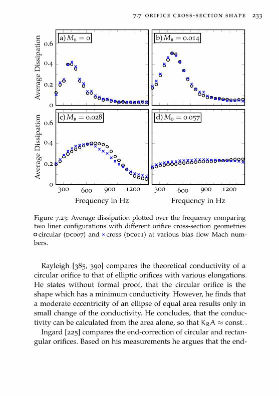
7.7 orifice cross-section shape 233
a) Mb = 0
0
0.2
0.4
0.6A
vera
geD
issi
pati
on b) Mb = 0.014
c) Mb = 0.028
300 600 900 12000
0.2
0.4
0.6
Frequency in Hz
Ave
rage
Dis
sipa
tion d) Mb = 0.057
300 600 900 1200
Frequency in Hz
Figure 7.23: Average dissipation plotted over the frequency comparingtwo liner configurations with different orifice cross-section geometries
circular (dc007) and cross (dc011) at various bias flow Mach num-bers.
Rayleigh [385, 390] compares the theoretical conductivity of acircular orifice to that of elliptic orifices with various elongations.He states without formal proof, that the circular orifice is theshape which has a minimum conductivity. However, he finds thata moderate eccentricity of an ellipse of equal area results only insmall change of the conductivity. He concludes, that the conduc-tivity can be calculated from the area alone, so that KRA ≈ const. .
Ingard [225] compares the end-correction of circular and rectan-gular orifices. Based on his measurements he argues that the end-
234 parameter study
correction scales with the orifice area only, confirming Rayleigh’stheoretical assumption.
Morfey [336] reviews the work concerned with the influence oforifice shape on the sound transmission, which includes circular,elliptic, and rectangular cross-sections. In conclusion, he estimatesthe conductivity of an orifice of arbitrary shape in terms of perime-ter P and area A with
KR =π
2P
ln (P2/A). (7.4)
For a circular orifice Equation (7.4) yields KR ≈ 3.9r, which agreeswith Rayleigh’s result6 KR = 4
√A/π = 4r. However, accord-
ing to Morfey Equation (7.4) gives more appropriate results forvery long, narrow openings, where the longest dimension remainssmall in comparison with the wavelength. Inserting the dimen-sions of the circular and cross-shaped orifices from Table 7.5 yieldsa slightly different conductivity of 4.85 mm and 5.61 mm, respec-tively. Instead, using the hydraulic diameter to calculate the con-ductivity of the cross-shaped orifice yields KR = 4.54 mm, whichmatches slightly better to the circular geometry.
Chanaud [89] presents a theoretical study on geometry effectson the resonance frequency of Helmholtz resonators. Amongstother things, he studies the influence of the orifice cross-sectiongeometry. He treats a circular, square, rectangular, and three differ-ent cross-shaped orifices, all of which have equal area. His resultssuggest that the orifice cross-section shape is not highly signifi-cant.
Grace et al. [181] numerically calculates the Rayleigh conduc-tivity for a variety of orifice shapes for both one-sided and two-sided grazing flows. The cross-section geometries includes a cir-cle, square, various triangles, and a crown7 with equal maximum
6 Morfey treats only one side of the orifice, so this equals twice the valueobtained by Rayleigh for both sides.
7 The crown is an orifice with square cross-section and triangular serratedleading or trailing edge, see Figure 2.5i.
7.7 orifice cross-section shape 235
dimension in streamwise direction. Accounting for the differentopen areas of the orifices, the conductivities are normalized withrespect to
√A. The results are found not to vary significantly
with the orifice shape, where the triangular shapes produced thelargest differences compared to a circular orifice.
Ahuja and Gaeta [7, 169] performed an experimental study onthe effect of the orifice shape on its acoustic impedance. The cross-section geometries of the orifices are circular, square, triangular,star-shaped, and eye-shaped8 with equivalent area. The length ofthe perimeter is more than doubled between the circular and star-shaped orifice. Measurements were done at low and high soundpressure levels. They find that at low incident sound amplitudesthe resistance increases with the perimeter, so that orifices withshapes that are significantly different from circular yield a higherabsorption. However, at higher amplitudes the resistance appearsto be independent of the orifice shape. They specify an orifice ve-locity of 0.5 m/s as limiting value where the transition occurs.
Based on the literature, the orifice cross-section shape seemsto have a minor effect on the acoustic properties in stationarymedium or with grazing flow. The findings of Ahuja and Gaeta [7,169] at high amplitudes suggest that any effect vanishes whenthere is a bias flow present. This is confirmed by the experimentalresults here. As a consequence it seems to be sufficient to matchthe orifice area when dealing with different cross-section geome-tries.
Rayleigh [385, 390] and Morfey [336] expect a more substantialchange of the conductivity for a long narrow slit when comparedto a circular orifice. However, no data is available that providessuch a comparison.
8 This is achieved by sliding a perforation consisting of circular orifices overanother identical perforation, see Figure 2.5j. Ahuja and Gaeta [7, 169] referto this shape as stepped-oval geometry.
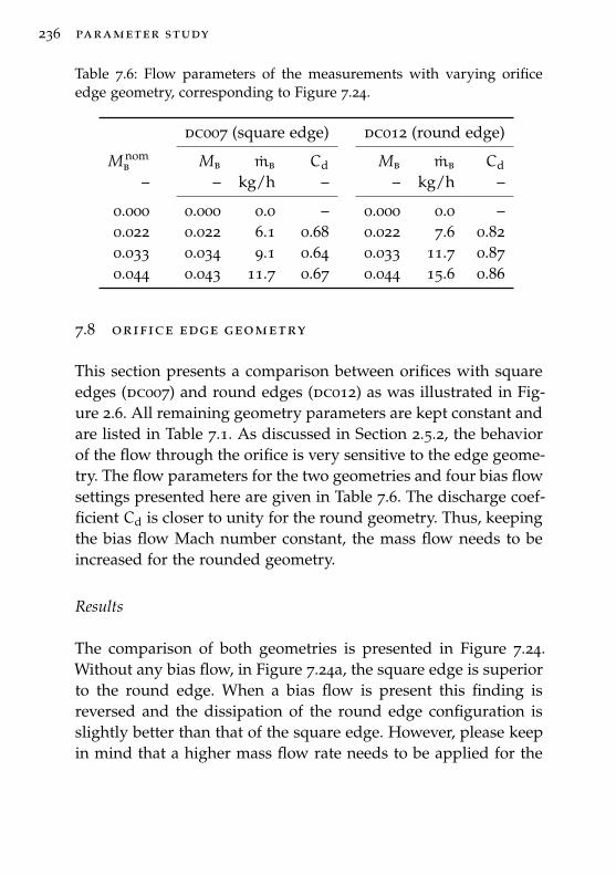
236 parameter study
Table 7.6: Flow parameters of the measurements with varying orificeedge geometry, corresponding to Figure 7.24.
dc007 (square edge) dc012 (round edge)
M nomb Mb mb Cd Mb mb Cd
– – kg/h – – kg/h –
0.000 0.000 0.0 – 0.000 0.0 –0.022 0.022 6.1 0.68 0.022 7.6 0.820.033 0.034 9.1 0.64 0.033 11.7 0.870.044 0.043 11.7 0.67 0.044 15.6 0.86
7.8 orifice edge geometry
This section presents a comparison between orifices with squareedges (dc007) and round edges (dc012) as was illustrated in Fig-ure 2.6. All remaining geometry parameters are kept constant andare listed in Table 7.1. As discussed in Section 2.5.2, the behaviorof the flow through the orifice is very sensitive to the edge geome-try. The flow parameters for the two geometries and four bias flowsettings presented here are given in Table 7.6. The discharge coef-ficient Cd is closer to unity for the round geometry. Thus, keepingthe bias flow Mach number constant, the mass flow needs to beincreased for the rounded geometry.
Results
The comparison of both geometries is presented in Figure 7.24.Without any bias flow, in Figure 7.24a, the square edge is superiorto the round edge. When a bias flow is present this finding isreversed and the dissipation of the round edge configuration isslightly better than that of the square edge. However, please keepin mind that a higher mass flow rate needs to be applied for the
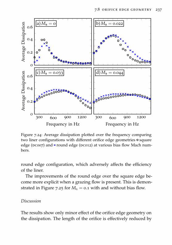
7.8 orifice edge geometry 237
a) Mb = 0
0
0.2
0.4
0.6A
vera
geD
issi
pati
on b) Mb = 0.022
c) Mb = 0.033
300 600 900 12000
0.2
0.4
0.6
Frequency in Hz
Ave
rage
Dis
sipa
tion d) Mb = 0.044
300 600 900 1200
Frequency in Hz
Figure 7.24: Average dissipation plotted over the frequency comparingtwo liner configurations with different orifice edge geometries squareedge (dc007) and round edge (dc012) at various bias flow Mach num-bers.
round edge configuration, which adversely affects the efficiencyof the liner.
The improvements of the round edge over the square edge be-come more explicit when a grazing flow is present. This is demon-strated in Figure 7.25 for Mg = 0.1 with and without bias flow.
Discussion
The results show only minor effect of the orifice edge geometry onthe dissipation. The length of the orifice is effectively reduced by
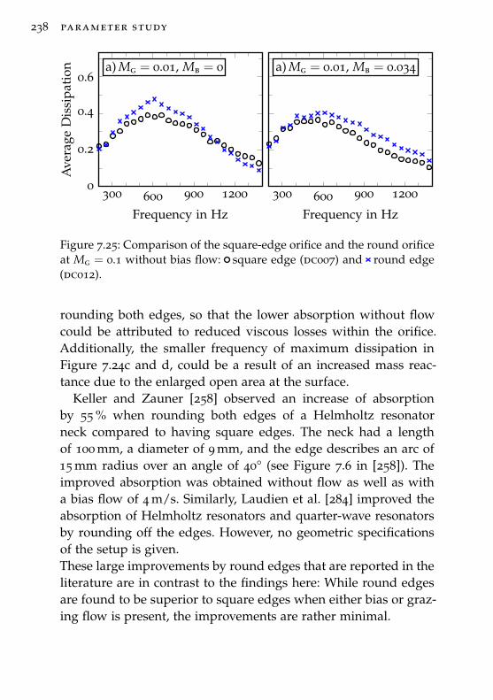
238 parameter study
a) Mg = 0.01, Mb = 0
300 600 900 12000
0.2
0.4
0.6
Frequency in Hz
Ave
rage
Dis
sipa
tion a) Mg = 0.01, Mb = 0.034
300 600 900 1200
Frequency in Hz
Figure 7.25: Comparison of the square-edge orifice and the round orificeat Mg = 0.1 without bias flow: square edge (dc007) and round edge(dc012).
rounding both edges, so that the lower absorption without flowcould be attributed to reduced viscous losses within the orifice.Additionally, the smaller frequency of maximum dissipation inFigure 7.24c and d, could be a result of an increased mass reac-tance due to the enlarged open area at the surface.
Keller and Zauner [258] observed an increase of absorptionby 55 % when rounding both edges of a Helmholtz resonatorneck compared to having square edges. The neck had a lengthof 100 mm, a diameter of 9 mm, and the edge describes an arc of15 mm radius over an angle of 40° (see Figure 7.6 in [258]). Theimproved absorption was obtained without flow as well as witha bias flow of 4 m/s. Similarly, Laudien et al. [284] improved theabsorption of Helmholtz resonators and quarter-wave resonatorsby rounding off the edges. However, no geometric specificationsof the setup is given.These large improvements by round edges that are reported in theliterature are in contrast to the findings here: While round edgesare found to be superior to square edges when either bias or graz-ing flow is present, the improvements are rather minimal.
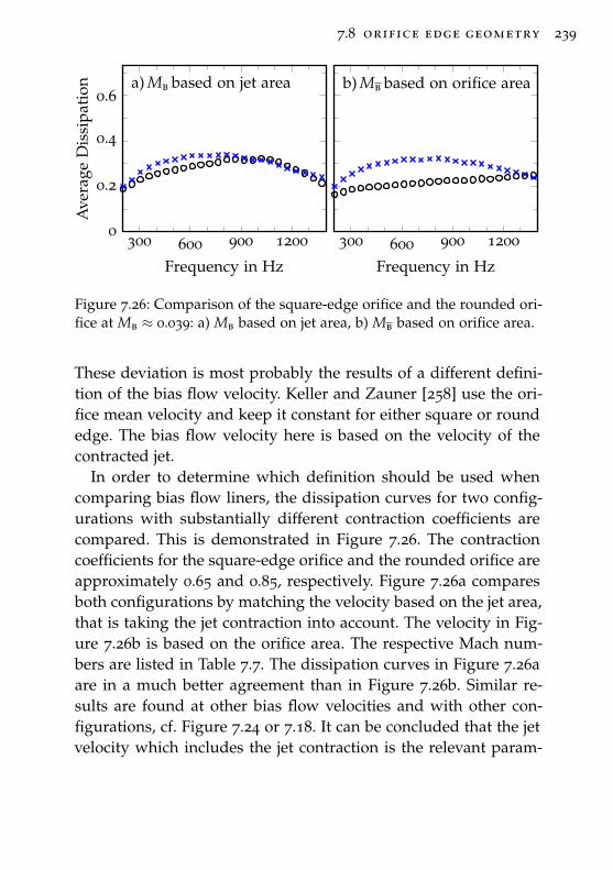
7.8 orifice edge geometry 239
a) Mb based on jet area
300 600 900 12000
0.2
0.4
0.6
Frequency in Hz
Ave
rage
Dis
sipa
tion b) Mb based on orifice area
300 600 900 1200
Frequency in Hz
Figure 7.26: Comparison of the square-edge orifice and the rounded ori-fice at Mb ≈ 0.039: a) Mb based on jet area, b) Mb based on orifice area.
These deviation is most probably the results of a different defini-tion of the bias flow velocity. Keller and Zauner [258] use the ori-fice mean velocity and keep it constant for either square or roundedge. The bias flow velocity here is based on the velocity of thecontracted jet.
In order to determine which definition should be used whencomparing bias flow liners, the dissipation curves for two config-urations with substantially different contraction coefficients arecompared. This is demonstrated in Figure 7.26. The contractioncoefficients for the square-edge orifice and the rounded orifice areapproximately 0.65 and 0.85, respectively. Figure 7.26a comparesboth configurations by matching the velocity based on the jet area,that is taking the jet contraction into account. The velocity in Fig-ure 7.26b is based on the orifice area. The respective Mach num-bers are listed in Table 7.7. The dissipation curves in Figure 7.26aare in a much better agreement than in Figure 7.26b. Similar re-sults are found at other bias flow velocities and with other con-figurations, cf. Figure 7.24 or 7.18. It can be concluded that the jetvelocity which includes the jet contraction is the relevant param-
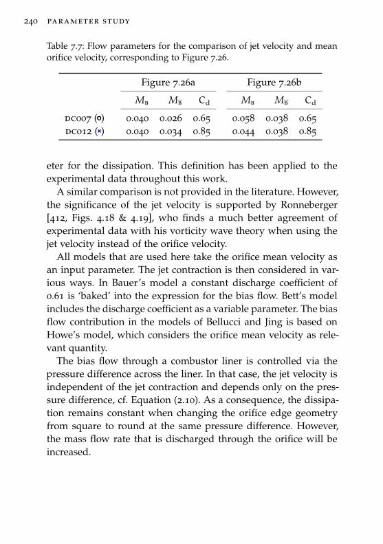
240 parameter study
Table 7.7: Flow parameters for the comparison of jet velocity and meanorifice velocity, corresponding to Figure 7.26.
Figure 7.26a Figure 7.26b
Mb Mb Cd Mb Mb Cd
dc007 ( ) 0.040 0.026 0.65 0.058 0.038 0.65dc012 ( ) 0.040 0.034 0.85 0.044 0.038 0.85
eter for the dissipation. This definition has been applied to theexperimental data throughout this work.
A similar comparison is not provided in the literature. However,the significance of the jet velocity is supported by Ronneberger[412, Figs. 4.18 & 4.19], who finds a much better agreement ofexperimental data with his vorticity wave theory when using thejet velocity instead of the orifice velocity.
All models that are used here take the orifice mean velocity asan input parameter. The jet contraction is then considered in var-ious ways. In Bauer’s model a constant discharge coefficient of0.61 is ‘baked’ into the expression for the bias flow. Bett’s modelincludes the discharge coefficient as a variable parameter. The biasflow contribution in the models of Bellucci and Jing is based onHowe’s model, which considers the orifice mean velocity as rele-vant quantity.
The bias flow through a combustor liner is controlled via thepressure difference across the liner. In that case, the jet velocity isindependent of the jet contraction and depends only on the pres-sure difference, cf. Equation (2.10). As a consequence, the dissipa-tion remains constant when changing the orifice edge geometryfrom square to round at the same pressure difference. However,the mass flow rate that is discharged through the orifice will beincreased.
7.9 orifice angle 241
Table 7.8: Geometry parameters regarding the orifice angle.
Configuration hc006 hc007 hc008
Orifice Angle deg 90 60 30Wall Thickness mm 2 2 2Orifice Length mm 2 2.3 4
7.9 orifice angle
Inclining the orifices from their 90° angle results in an asymmet-ric behavior, so that the amount of dissipated acoustic energy de-pends on the direction of sound propagation relative to the incli-nation angle. Here, the orifices are inclined in positive x-direction,so that while reducing the inclination angle the direction of thebias flow injection aligns more and more with the grazing flow.Keeping the wall thickness constant increases the orifice lengthfor angles other than 90°, as specified in Equation (2.1). These ge-ometric features are listed in Table 7.8.
Results
The influence of the inclination angle on the directional perfor-mance of the liner is shown in Figure 7.27. The dissipation curvesfor sound propagating in positive and negative direction are com-pared for liners of different inclination angles. The curves for the90° angle (no inclination) are identical, as is expected for a sym-metric configuration without grazing flow. Decreasing the incli-nation angle increases the dissipation of sound propagating inpositive x-direction, while it decreases the dissipation of soundpropagating in the opposite direction. It was shown before (seeFigure 7.11) that a grazing flow has the opposite effect. Lookingat inclined orifices in a grazing flow environment (the right col-umn in Figure 7.27) reveals that both effects counteract each other
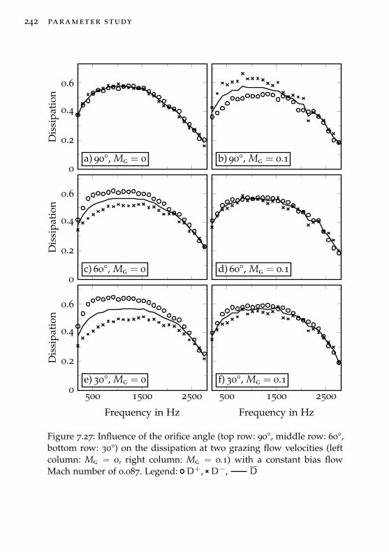
242 parameter study
a) 90°, Mg = 00
0.2
0.4
0.6
Dis
sipa
tion
b) 90°, Mg = 0.1
c) 60°, Mg = 00
0.2
0.4
0.6
Dis
sipa
tion
d) 60°, Mg = 0.1
e) 30°, Mg = 0
500 1500 25000
0.2
0.4
0.6
Frequency in Hz
Dis
sipa
tion
f) 30°, Mg = 0.1
500 1500 2500
Frequency in Hz
Figure 7.27: Influence of the orifice angle (top row: 90°, middle row: 60°,bottom row: 30°) on the dissipation at two grazing flow velocities (leftcolumn: Mg = 0, right column: Mg = 0.1) with a constant bias flowMach number of 0.087. Legend: D+, D−, D
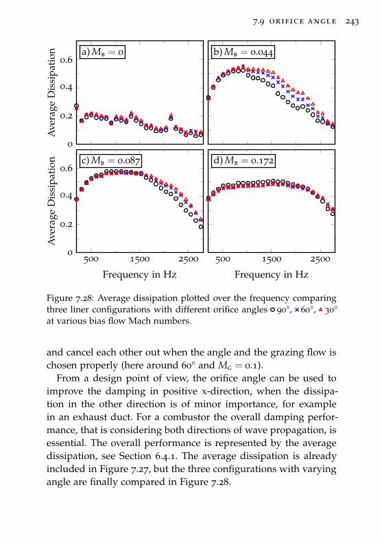
7.9 orifice angle 243
a) Mb = 0
0
0.2
0.4
0.6A
vera
geD
issi
pati
on b) Mb = 0.044
c) Mb = 0.087
500 1500 25000
0.2
0.4
0.6
Frequency in Hz
Ave
rage
Dis
sipa
tion d) Mb = 0.172
500 1500 2500
Frequency in Hz
Figure 7.28: Average dissipation plotted over the frequency comparingthree liner configurations with different orifice angles 90°, 60°, 30°at various bias flow Mach numbers.
and cancel each other out when the angle and the grazing flow ischosen properly (here around 60° and Mg = 0.1).
From a design point of view, the orifice angle can be used toimprove the damping in positive x-direction, when the dissipa-tion in the other direction is of minor importance, for examplein an exhaust duct. For a combustor the overall damping perfor-mance, that is considering both directions of wave propagation, isessential. The overall performance is represented by the averagedissipation, see Section 6.4.1. The average dissipation is alreadyincluded in Figure 7.27, but the three configurations with varyingangle are finally compared in Figure 7.28.
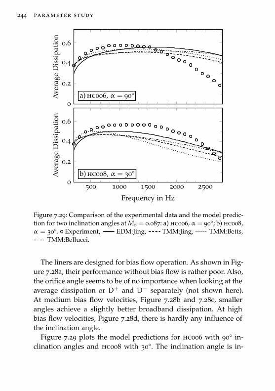
244 parameter study
a) hc006, α = 90°0
0.2
0.4
0.6
Ave
rage
Dis
sipa
tion
b) hc008, α = 30°
500 1000 1500 2000 25000
0.2
0.4
0.6
Frequency in Hz
Ave
rage
Dis
sipa
tion
Figure 7.29: Comparison of the experimental data and the model predic-tion for two inclination angles at Mb = 0.087: a) hc006, α = 90°; b) hc008,α = 30°. Experiment, EDM:Jing, TMM:Jing, TMM:Betts,
TMM:Bellucci.
The liners are designed for bias flow operation. As shown in Fig-ure 7.28a, their performance without bias flow is rather poor. Also,the orifice angle seems to be of no importance when looking at theaverage dissipation or D+ and D− separately (not shown here).At medium bias flow velocities, Figure 7.28b and 7.28c, smallerangles achieve a slightly better broadband dissipation. At highbias flow velocities, Figure 7.28d, there is hardly any influence ofthe inclination angle.
Figure 7.29 plots the model predictions for hc006 with 90° in-clination angles and hc008 with 30°. The inclination angle is in-
7.9 orifice angle 245
cluded in the models by simply using the orifice length (Equa-tion (2.1)) instead of the wall thickness. The behavior of the mod-els is rather similar. As the angle is included by adjusting theorifice length, the predicted effect is equivalent to increasing thewall thickness and keeping the angle constant, cf. Section 7.6. Theresult is a reduction of the broadband absorption with increas-ing orifice length/decreasing angle. However, the experimentalresults show the opposite effect. Unfortunately, the agreement be-tween models and experiment is poor at frequencies > 1500 Hz,already for the standard 90° configuration. Thus, a detailed inter-pretation of the model results is difficult.
Discussion
Eldredge and Dowling [142] include the inclination angle in theiranalysis by simply using the orifice length, instead of the wallthickness (cf. Figure 2.7b). The same approach was used by El-dredge et al. [141] and compared to data obtained from a large-eddy simulation of an inclined bias flow orifice. They found thatthe agreement can be further improved by considering that the ac-tual openings of the orifice are elliptical and not circular when it isinclined, i. e. the area is slightly larger. This is taken into accountby an empirical correction factor of 0.75, so that the corrected ori-fice length for an inclined orifice is given by
l = 0.75 t/ sin α (7.5)
Andreini et al. [17] report that any effect of the inclination angledisappears with increasing bias flow, while the 90° orientation isslightly superior at low bias flow velocities. However, their mea-surements include a grazing flow which might counteract on theeffect of the inclination angle as shown in Figure 7.27. They arecomparing the results to EDM:Jing and yield good agreement9.
9 Eq. (6) of [17] only includes the wall thickness and not the orifice length.However, this must be a spelling mistake as the predictions for the two con-
246 parameter study
Here, the largest effect is found to be at higher frequencies. Thedata of Andreini et al. [17] is limited to frequencies below 1500 Hz.
Laurens et al. [285] present a mathematical treatment of theRayleigh conductivity for inclined orifices in the absence of flow.They show that the effect of the orifice angle is not entirely cap-tured by the intuitive extension of the length, as described byEquation (2.1) and applied previously [17, 141, 142, 328], but thatthe increased area of the elliptical openings needs to be consid-ered as well10. Laurens et al. [285] derive upper and lower boundsof the Rayleigh conductivity of an inclined orifice with circularcross-section and elliptical openings11. They find that the empiri-cal correction of Eldredge et al. [141] falls within these bounds, infact it is close to the mean value of the upper and lower bounds.This good agreement is quite surprising as the bounds in [285] arederived for stationary fluid and the simulation in [141] includes abias and grazing flow.
The effect of the orifice length alone (without inclination) wasdiscussed in Section 7.6. While the inclination angle also increasesthe length, it seems to have the opposite effect on the dissipation.This hints to an additional effect that has not been accounted forin the models. As suggested in the literature, the elliptical open-ing should be considered as well. This can be done by applyingthe correction factor given by Eldredge et al. [141]. The correctionfactor is presumed to be dependent on the inclination angle. How-ever, it was determined for a 30° configuration12, which is avail-able here as well. Anyhow, the angle of 30° doubles the lengthcompared to the 90° configuration. Applying a correction factor
figurations produce different results when the inclination angle is the onlymodified parameter.
10 This was already suggested by Eldredge et al. [141], who applied an empiri-cal correction (cf. Equation (7.5)).
11 They extend their treatment to other geometries as well, but this is the rele-vant configuration for gas turbine combustors.
12 Please note, that the angle in [141] is measured from the wall normal, so that60° in [141] is equivalent to 30° here.
7.10 double-skin configuration 247
of 0.75 for the elliptical opening will produce a result that lies in-between the results for 30° and 90° without the correction factor,but will not surpass the 90° result. As a consequence the effectwill be weakened, but not be turned around.Section 7.6 has shown that the influence of the wall thickness dis-appears at high bias flow velocities. When transferring this find-ing to the inclined orifice, it could be proposed to keep the rele-vant length constant to the wall thickness and apply a correctionfor the increased opening area only. This would yield the desiredeffect for a bias flow setup.
7.10 double-skin configuration
A double-skin configuration allows to reduce the bias flow veloc-ity of the damping liner when the total pressure drop is fixed, asit is in a combustor. The bias flow velocity through the dampingliner is then determined by the open-area-ratio between dampingand metering liner. The velocity through the metering liner is typ-ically much higher.
Results
The experimental results in Figure 7.30 demonstrate this effect fortwo double-skin configurations. The open-area-ratio of both con-figurations is 0.3. Without any bias flow the dissipation curve ex-hibits two maxima (one maximum in Figure 7.30a is expected justbeyond the plotted frequency range). The frequencies of these twomaxima correspond to the Helmholtz resonances of the dampingand metering liners and their associated cavities, so that each max-imum can be related to the one or the other. Here, the maxima atthe higher frequencies correspond to the damping liner. The peaksassociated with the metering liner are eliminated when applyinga damping liner bias flow of Mb = 0.014. At the given open-area-ratio, that corresponds to a metering liner bias flow Mach number
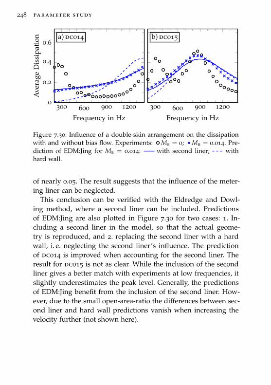
248 parameter study
a) dc014
300 600 900 12000
0.2
0.4
0.6
Frequency in Hz
Ave
rage
Dis
sipa
tion b) dc015
300 600 900 1200
Frequency in Hz
Figure 7.30: Influence of a double-skin arrangement on the dissipationwith and without bias flow. Experiments: Mb = 0; Mb = 0.014. Pre-diction of EDM:Jing for Mb = 0.014: with second liner; withhard wall.
of nearly 0.05. The result suggests that the influence of the meter-ing liner can be neglected.
This conclusion can be verified with the Eldredge and Dowl-ing method, where a second liner can be included. Predictionsof EDM:Jing are also plotted in Figure 7.30 for two cases: 1. In-cluding a second liner in the model, so that the actual geome-try is reproduced, and 2. replacing the second liner with a hardwall, i. e. neglecting the second liner’s influence. The predictionof dc014 is improved when accounting for the second liner. Theresult for dc015 is not as clear. While the inclusion of the secondliner gives a better match with experiments at low frequencies, itslightly underestimates the peak level. Generally, the predictionsof EDM:Jing benefit from the inclusion of the second liner. How-ever, due to the small open-area-ratio the differences between sec-ond liner and hard wall predictions vanish when increasing thevelocity further (not shown here).
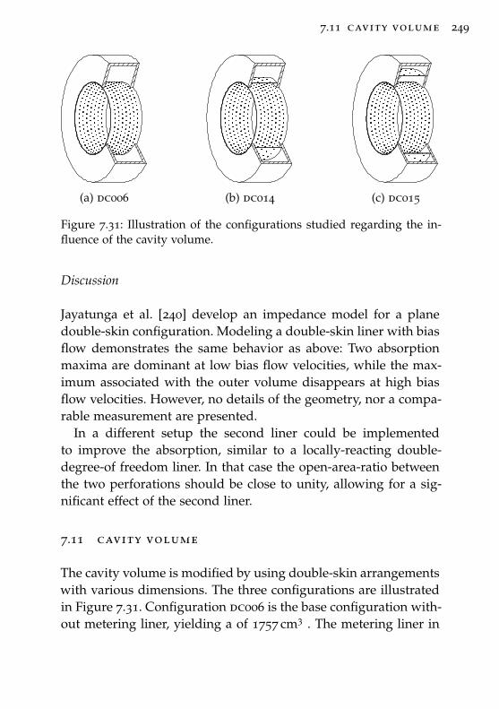
7.11 cavity volume 249
(a) dc006 (b) dc014 (c) dc015
Figure 7.31: Illustration of the configurations studied regarding the in-fluence of the cavity volume.
Discussion
Jayatunga et al. [240] develop an impedance model for a planedouble-skin configuration. Modeling a double-skin liner with biasflow demonstrates the same behavior as above: Two absorptionmaxima are dominant at low bias flow velocities, while the max-imum associated with the outer volume disappears at high biasflow velocities. However, no details of the geometry, nor a compa-rable measurement are presented.
In a different setup the second liner could be implementedto improve the absorption, similar to a locally-reacting double-degree-of freedom liner. In that case the open-area-ratio betweenthe two perforations should be close to unity, allowing for a sig-nificant effect of the second liner.
7.11 cavity volume
The cavity volume is modified by using double-skin arrangementswith various dimensions. The three configurations are illustratedin Figure 7.31. Configuration dc006 is the base configuration with-out metering liner, yielding a of 1757 cm3 . The metering liner in
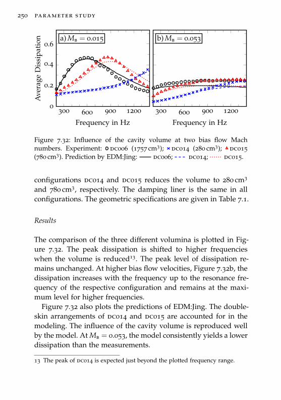
250 parameter study
a) Mb = 0.015
300 600 900 12000
0.2
0.4
0.6
Frequency in Hz
Ave
rage
Dis
sipa
tion b) Mb = 0.053
300 600 900 1200
Frequency in Hz
Figure 7.32: Influence of the cavity volume at two bias flow Machnumbers. Experiment: dc006 (1757 cm3); dc014 (280 cm3); dc015(780 cm3). Prediction by EDM:Jing: dc006; dc014; dc015.
configurations dc014 and dc015 reduces the volume to 280 cm3
and 780 cm3, respectively. The damping liner is the same in allconfigurations. The geometric specifications are given in Table 7.1.
Results
The comparison of the three different volumina is plotted in Fig-ure 7.32. The peak dissipation is shifted to higher frequencieswhen the volume is reduced13. The peak level of dissipation re-mains unchanged. At higher bias flow velocities, Figure 7.32b, thedissipation increases with the frequency up to the resonance fre-quency of the respective configuration and remains at the maxi-mum level for higher frequencies.
Figure 7.32 also plots the predictions of EDM:Jing. The double-skin arrangements of dc014 and dc015 are accounted for in themodeling. The influence of the cavity volume is reproduced wellby the model. At Mb = 0.053, the model consistently yields a lowerdissipation than the measurements.
13 The peak of dc014 is expected just beyond the plotted frequency range.
7.11 cavity volume 251
Discussion
As discussed in Section 7.2, the frequency of maximum dissipa-tion is related to a resonance frequency of the system. When alldimensions are much smaller than the wave length, this is typi-cally a Helmholtz resonance. In that case, the resonance frequencyis directly dependent on the cavity volume. This relationship is anobvious conclusion from Figure 7.32a. The theoretical Helmholtzresonance frequencies for the three configurations are included inTable 7.9.
The bias flow shifts the resonance frequency to higher values14,so that the theoretical values in Table 7.9 do not exactly matchwith the dissipation maxima in Figure 7.32a. This is due to thedecrease of the reactance by the bias flow (see discussion in Sec-tion 7.2). The reduction of the reactance seems to be a generallyaccepted fact, but the literature does not provide a collective opin-ion on the more specific behavior. While some models do not in-clude any influence on the reactance at all, other models predictvery different strengths of the phenomena (see Figure 4.9). Wester-velt [491] found that the reactance ultimately becomes zero whena bias flow is present. The impedance measurements of Jing andSun [242] demonstrate the behavior of the reactance, and in fact itis close to zero at a certain bias flow setting. However, this behav-ior is underestimated by the Jing model as well as the numericalmodel presented in [242].
Assuming the reactance becomes zero at sufficiently high biasflow velocities, this would yield a resonance frequency of infinity.In fact, at Mb = 0.053 in Figure 7.32b no resonance is visible. In-terestingly enough, the dissipation increases with the frequencyuntil it reaches its maxium at the theoretical no flow Helmholtzresonance and remains constant at higher frequencies. This behav-ior can not only be observed for the three configurations in Fig-
14 The second liner in configurations dc014 and dc015 invalidates the hard-wallassumption, so that the measured resonance frequencies are slightly higherthan the theoretical ones already without flow (cf. Figure 7.30).
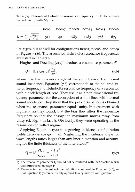
252 parameter study
Table 7.9: Theoretical Helmholtz resonance frequency in Hz for a hard-walled cavity with Mb = 0.
dc006 dc007 dc008 dc014 dc015 hc006
fr =c
2π
√AopenVleff
512 400 985 1283 768 679
ure 7.32b, but as well for configurations dc007, dc008, and dc009in Figure 7.18d. The associated Helmholtz resonance frequenciesare listed in Table 7.9.
Hughes and Dowling [219] introduce a resonance parameter15
Q = (k s cos θ)2 dc
2r, (7.6)
where θ is the incidence angle of the sound wave. For normalsound incidence, Equation (7.6) corresponds to the squared ra-tio of frequency to Helmholtz resonance frequency of a resonatorwith a neck length of zero. They use it as a non-dimensional fre-quency parameter for the absorption of a thin liner with normalsound incidence. They show that the peak dissipation is obtainedwhen the resonance parameter equals unity. In agreement withFigure 7.32a they found, that the bias flow alters the resonancefrequency, so that the absorption maximum moves away fromunity (cf. Fig. 3 in [219]). Obviously, they were operating in theresonance controlled regime.
Applying Equation (7.6) to a grazing incidence configurationyields zero (as cos 90◦ = 0). Neglecting the incidence angle forwave lengths much larger than any liner dimension and account-ing for the finite thickness of the liner yields16
Q = k2 Vleff
Aopen=
(f
fr
)2
. (7.7)
15 The resonance parameter Q should not be confused with the Q factor, whichwas introduced on page 43.
16 Please note the different volume definition compared to Equation (7.6), sothat Equation (7.7) can be readily applied to a cylindrical configuration.
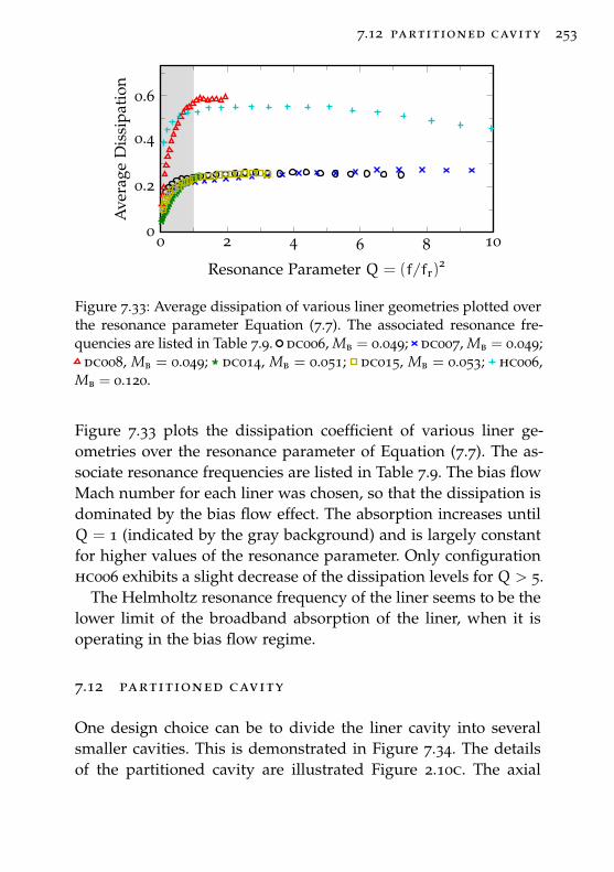
7.12 partitioned cavity 253
0 2 4 6 8 100
0.2
0.4
0.6
Resonance Parameter Q = (f/fr)2
Ave
rage
Dis
sipa
tion
Figure 7.33: Average dissipation of various liner geometries plotted overthe resonance parameter Equation (7.7). The associated resonance fre-quencies are listed in Table 7.9. dc006, Mb = 0.049; dc007, Mb = 0.049;
dc008, Mb = 0.049; dc014, Mb = 0.051; dc015, Mb = 0.053; hc006,Mb = 0.120.
Figure 7.33 plots the dissipation coefficient of various liner ge-ometries over the resonance parameter of Equation (7.7). The as-sociate resonance frequencies are listed in Table 7.9. The bias flowMach number for each liner was chosen, so that the dissipation isdominated by the bias flow effect. The absorption increases untilQ = 1 (indicated by the gray background) and is largely constantfor higher values of the resonance parameter. Only configurationhc006 exhibits a slight decrease of the dissipation levels for Q > 5.
The Helmholtz resonance frequency of the liner seems to be thelower limit of the broadband absorption of the liner, when it isoperating in the bias flow regime.
7.12 partitioned cavity
One design choice can be to divide the liner cavity into severalsmaller cavities. This is demonstrated in Figure 7.34. The detailsof the partitioned cavity are illustrated Figure 2.10c. The axial
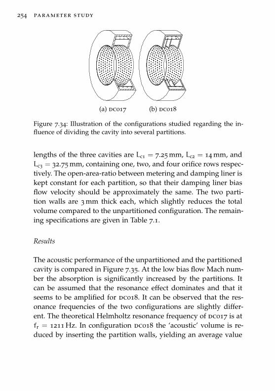
254 parameter study
(a) dc017 (b) dc018
Figure 7.34: Illustration of the configurations studied regarding the in-fluence of dividing the cavity into several partitions.
lengths of the three cavities are Lc1 = 7.25 mm, Lc2 = 14 mm, andLc3 = 32.75 mm, containing one, two, and four orifice rows respec-tively. The open-area-ratio between metering and damping liner iskept constant for each partition, so that their damping liner biasflow velocity should be approximately the same. The two parti-tion walls are 3 mm thick each, which slightly reduces the totalvolume compared to the unpartitioned configuration. The remain-ing specifications are given in Table 7.1.
Results
The acoustic performance of the unpartitioned and the partitionedcavity is compared in Figure 7.35. At the low bias flow Mach num-ber the absorption is significantly increased by the partitions. Itcan be assumed that the resonance effect dominates and that itseems to be amplified for dc018. It can be observed that the res-onance frequencies of the two configurations are slightly differ-ent. The theoretical Helmholtz resonance frequency of dc017 is atfr = 1211 Hz. In configuration dc018 the ‘acoustic’ volume is re-duced by inserting the partition walls, yielding an average value
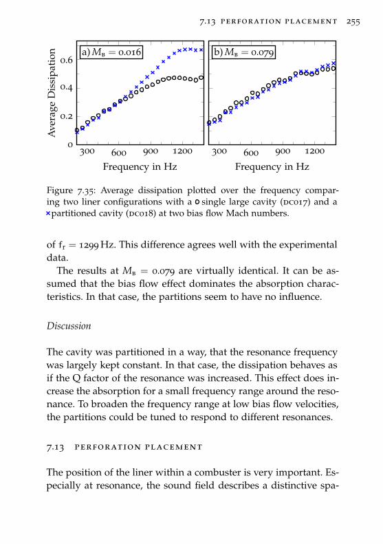
7.13 perforation placement 255
a) Mb = 0.016
300 600 900 12000
0.2
0.4
0.6
Frequency in Hz
Ave
rage
Dis
sipa
tion b) Mb = 0.079
300 600 900 1200
Frequency in Hz
Figure 7.35: Average dissipation plotted over the frequency compar-ing two liner configurations with a single large cavity (dc017) and a
partitioned cavity (dc018) at two bias flow Mach numbers.
of fr = 1299 Hz. This difference agrees well with the experimentaldata.
The results at Mb = 0.079 are virtually identical. It can be as-sumed that the bias flow effect dominates the absorption charac-teristics. In that case, the partitions seem to have no influence.
Discussion
The cavity was partitioned in a way, that the resonance frequencywas largely kept constant. In that case, the dissipation behaves asif the Q factor of the resonance was increased. This effect does in-crease the absorption for a small frequency range around the reso-nance. To broaden the frequency range at low bias flow velocities,the partitions could be tuned to respond to different resonances.
7.13 perforation placement
The position of the liner within a combuster is very important. Es-pecially at resonance, the sound field describes a distinctive spa-
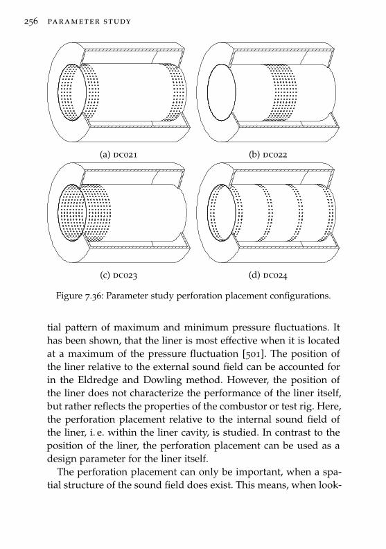
256 parameter study
(a) dc021 (b) dc022
(c) dc023 (d) dc024
Figure 7.36: Parameter study perforation placement configurations.
tial pattern of maximum and minimum pressure fluctuations. Ithas been shown, that the liner is most effective when it is locatedat a maximum of the pressure fluctuation [501]. The position ofthe liner relative to the external sound field can be accounted forin the Eldredge and Dowling method. However, the position ofthe liner does not characterize the performance of the liner itself,but rather reflects the properties of the combustor or test rig. Here,the perforation placement relative to the internal sound field ofthe liner, i. e. within the liner cavity, is studied. In contrast to theposition of the liner, the perforation placement can be used as adesign parameter for the liner itself.
The perforation placement can only be important, when a spa-tial structure of the sound field does exist. This means, when look-
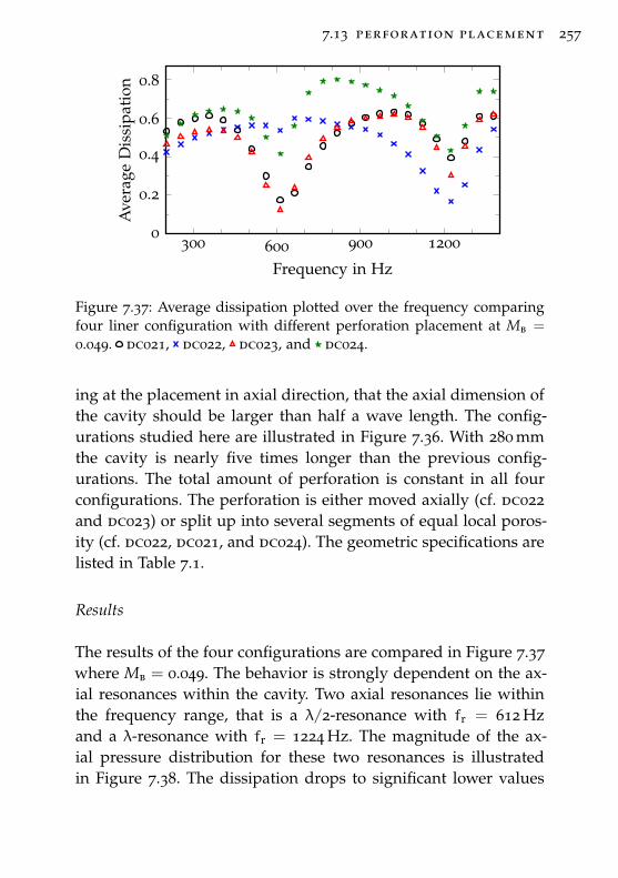
7.13 perforation placement 257
300 600 900 12000
0.2
0.4
0.6
0.8
Frequency in Hz
Ave
rage
Dis
sipa
tion
Figure 7.37: Average dissipation plotted over the frequency comparingfour liner configuration with different perforation placement at Mb =
0.049. dc021, dc022, dc023, and dc024.
ing at the placement in axial direction, that the axial dimension ofthe cavity should be larger than half a wave length. The config-urations studied here are illustrated in Figure 7.36. With 280 mmthe cavity is nearly five times longer than the previous config-urations. The total amount of perforation is constant in all fourconfigurations. The perforation is either moved axially (cf. dc022and dc023) or split up into several segments of equal local poros-ity (cf. dc022, dc021, and dc024). The geometric specifications arelisted in Table 7.1.
Results
The results of the four configurations are compared in Figure 7.37where Mb = 0.049. The behavior is strongly dependent on the ax-ial resonances within the cavity. Two axial resonances lie withinthe frequency range, that is a λ/2-resonance with fr = 612 Hzand a λ-resonance with fr = 1224 Hz. The magnitude of the ax-ial pressure distribution for these two resonances is illustratedin Figure 7.38. The dissipation drops to significant lower values
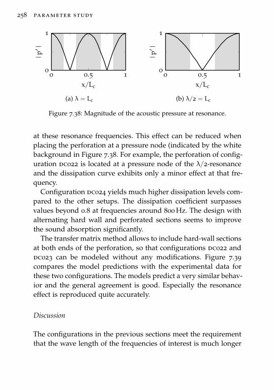
258 parameter study
0 0.5 10
1
x/Lc
|p′ |
(a) λ = Lc
0 0.5 10
1
x/Lc
|p′ |
(b) λ/2 = Lc
Figure 7.38: Magnitude of the acoustic pressure at resonance.
at these resonance frequencies. This effect can be reduced whenplacing the perforation at a pressure node (indicated by the whitebackground in Figure 7.38. For example, the perforation of config-uration dc022 is located at a pressure node of the λ/2-resonanceand the dissipation curve exhibits only a minor effect at that fre-quency.
Configuration dc024 yields much higher dissipation levels com-pared to the other setups. The dissipation coefficient surpassesvalues beyond 0.8 at frequencies around 800 Hz. The design withalternating hard wall and perforated sections seems to improvethe sound absorption significantly.
The transfer matrix method allows to include hard-wall sectionsat both ends of the perforation, so that configurations dc022 anddc023 can be modeled without any modifications. Figure 7.39compares the model predictions with the experimental data forthese two configurations. The models predict a very similar behav-ior and the general agreement is good. Especially the resonanceeffect is reproduced quite accurately.
Discussion
The configurations in the previous sections meet the requirementthat the wave length of the frequencies of interest is much longer
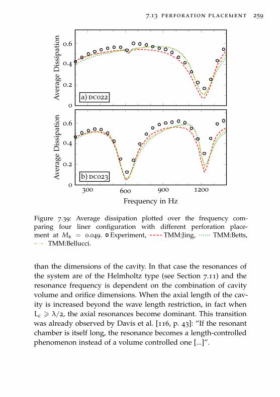
7.13 perforation placement 259
a) dc0220
0.2
0.4
0.6
Ave
rage
Dis
sipa
tion
b) dc023
300 600 900 12000
0.2
0.4
0.6
Frequency in Hz
Ave
rage
Dis
sipa
tion
Figure 7.39: Average dissipation plotted over the frequency com-paring four liner configuration with different perforation place-ment at Mb = 0.049. Experiment, TMM:Jing, TMM:Betts,
TMM:Bellucci.
than the dimensions of the cavity. In that case the resonances ofthe system are of the Helmholtz type (see Section 7.11) and theresonance frequency is dependent on the combination of cavityvolume and orifice dimensions. When the axial length of the cav-ity is increased beyond the wave length restriction, in fact whenLc > λ/2, the axial resonances become dominant. This transitionwas already observed by Davis et al. [116, p. 43]: “If the resonantchamber is itself long, the resonance becomes a length-controlledphenomenon instead of a volume controlled one [...]”.
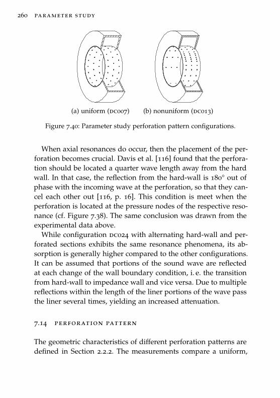
260 parameter study
(a) uniform (dc007) (b) nonuniform (dc013)
Figure 7.40: Parameter study perforation pattern configurations.
When axial resonances do occur, then the placement of the per-foration becomes crucial. Davis et al. [116] found that the perfora-tion should be located a quarter wave length away from the hardwall. In that case, the reflection from the hard-wall is 180° out ofphase with the incoming wave at the perforation, so that they can-cel each other out [116, p. 16]. This condition is meet when theperforation is located at the pressure nodes of the respective reso-nance (cf. Figure 7.38). The same conclusion was drawn from theexperimental data above.
While configuration dc024 with alternating hard-wall and per-forated sections exhibits the same resonance phenomena, its ab-sorption is generally higher compared to the other configurations.It can be assumed that portions of the sound wave are reflectedat each change of the wall boundary condition, i. e. the transitionfrom hard-wall to impedance wall and vice versa. Due to multiplereflections within the length of the liner portions of the wave passthe liner several times, yielding an increased attenuation.
7.14 perforation pattern
The geometric characteristics of different perforation patterns aredefined in Section 2.2.2. The measurements compare a uniform,
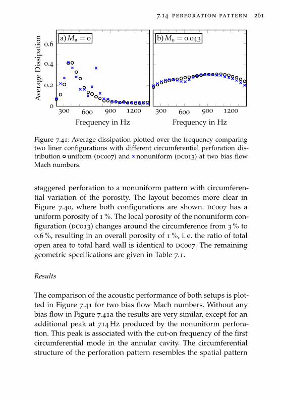
7.14 perforation pattern 261
a) Mb = 0
300 600 900 12000
0.2
0.4
0.6
Frequency in Hz
Ave
rage
Dis
sipa
tion b) Mb = 0.043
300 600 900 1200
Frequency in Hz
Figure 7.41: Average dissipation plotted over the frequency comparingtwo liner configurations with different circumferential perforation dis-tribution uniform (dc007) and nonuniform (dc013) at two bias flowMach numbers.
staggered perforation to a nonuniform pattern with circumferen-tial variation of the porosity. The layout becomes more clear inFigure 7.40, where both configurations are shown. dc007 has auniform porosity of 1 %. The local porosity of the nonuniform con-figuration (dc013) changes around the circumference from 3 % to0.6 %, resulting in an overall porosity of 1 %, i. e. the ratio of totalopen area to total hard wall is identical to dc007. The remaininggeometric specifications are given in Table 7.1.
Results
The comparison of the acoustic performance of both setups is plot-ted in Figure 7.41 for two bias flow Mach numbers. Without anybias flow in Figure 7.41a the results are very similar, except for anadditional peak at 714 Hz produced by the nonuniform perfora-tion. This peak is associated with the cut-on frequency of the firstcircumferential mode in the annular cavity. The circumferentialstructure of the perforation pattern resembles the spatial pattern
262 parameter study
of the mode, so that it is excited. The theoretical cut-on frequencyfor a hard-walled annulus of the same geometry is at 577 Hz. Thisfrequency is shifted to slightly higher values due to the perforatedwall at the inner radius (cf. [281]).
When a bias flow is present, as shown in Figure 7.41b, the reso-nance effects are largely suppressed and the broadband dampingdue to the bias flow dominates. The absorption of both geome-tries is rather similar, though two weak maxima are still visiblefor configuration dc013.
Discussion
The only experimental data that is found in the literature regard-ing a variation of the perforation pattern is concerned with theperforation aspect ratio, i. e. the abandonment of a square perfora-tion pattern for a rectangular pattern as illustrated in Figure 2.8.
Andreini et al. [17] present experimental results with two rect-angular perforation patterns, varying the perforation aspect ratiofrom sx/sθ =1.24 to 1.93. Both measurements are done with si-multaneous grazing and bias flow and retain a porosity of 1.82 %.The change in perforation aspect ratio did not show any influenceon the dissipation.
Lee et al. [288, 289] vary the perforation aspect ratio from anearly square configuration with sx/sθ =0.96 to a rectangularsetup, stretched in axial direction and compressed in circumfer-ential direction, resulting in sx/sθ =2.45. The porosity was keptconstant at 8.4 %. Without any flow they observe an increase ofthe transmission loss for the rectangular arrangement. This devi-ation between square and rectangular pattern becomes larger athigher frequencies.
This difference is somewhat surprising. When thinking in termsof porosity and diameter (which are both kept constant), the dif-ference would not be reproduced by any of the models. The actualorifice spacing seems to be important. The requirement for the ori-
7.14 perforation pattern 263
fices to act independently without interaction is given by d � s.For a square perforation pattern this limit is associated with acertain porosity σ 6 4 % (see Section 7.5). Due to the distortionof the orifice grid, the porosity cannot be used as a sole indica-tor for the interaction anymore. The spacing between the orificeshas to be evaluated in both directions separately. Translating theporosity requirement into a minimum spacing requirement yieldssmin/d > 4.4.
The spacing of the nearly square pattern is 7.6 mm and 7.9 mmin axial and circumferential direction, respectively. The rectangu-lar pattern is streched to 12 mm in axial direction and compressedto 4.9 mm in circumferential direction. The closer proximity of theorifices in circumferential direction could promote the interaction,even when the porosity is kept constant. The ratio of minimumspacing to orifice diameter is reduced from smin/d = 3 for thesquare pattern to 2 for the rectangular one. Both values fall shortof the required limit given above. The spacing to diameter ratiosof Andreini et al. [17] are smin/d = 4.7 and 5.9. This is larger thanthe ratios in Lee et al. [288, 289] and above the spacing require-ment.
The increased orifice interaction could be one possible explana-tion for the effect observed by Lee et al. [288, 289] and their con-tradictory results to Andreini et al. [17]. On the other hand, onemajor difference between the two studies is, that the experimentsof Lee et al. [288, 289] are performed without any flow, while bothbias and grazing flow is present in [17].
The experiments here have shown that the perforation patterncan be designed to promote certain cavity resonances. This isachieved by resembling the spatial structure of a cavity modewith the pattern of the perforation. This adds another degree offreedom, for example for the simultaneous absorption of multipletonal components. Naturally, this approach works only when the
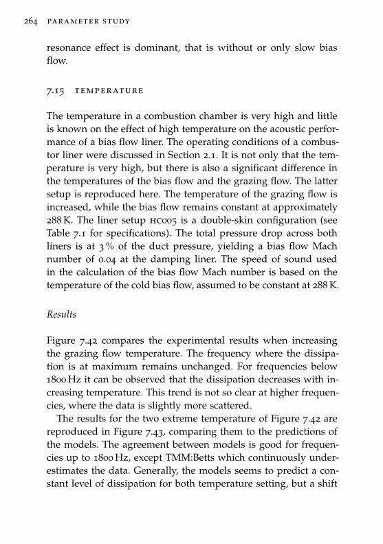
264 parameter study
resonance effect is dominant, that is without or only slow biasflow.
7.15 temperature
The temperature in a combustion chamber is very high and littleis known on the effect of high temperature on the acoustic perfor-mance of a bias flow liner. The operating conditions of a combus-tor liner were discussed in Section 2.1. It is not only that the tem-perature is very high, but there is also a significant difference inthe temperatures of the bias flow and the grazing flow. The lattersetup is reproduced here. The temperature of the grazing flow isincreased, while the bias flow remains constant at approximately288 K. The liner setup hc005 is a double-skin configuration (seeTable 7.1 for specifications). The total pressure drop across bothliners is at 3 % of the duct pressure, yielding a bias flow Machnumber of 0.04 at the damping liner. The speed of sound usedin the calculation of the bias flow Mach number is based on thetemperature of the cold bias flow, assumed to be constant at 288 K.
Results
Figure 7.42 compares the experimental results when increasingthe grazing flow temperature. The frequency where the dissipa-tion is at maximum remains unchanged. For frequencies below1800 Hz it can be observed that the dissipation decreases with in-creasing temperature. This trend is not so clear at higher frequen-cies, where the data is slightly more scattered.
The results for the two extreme temperature of Figure 7.42 arereproduced in Figure 7.43, comparing them to the predictions ofthe models. The agreement between models is good for frequen-cies up to 1800 Hz, except TMM:Betts which continuously under-estimates the data. Generally, the models seems to predict a con-stant level of dissipation for both temperature setting, but a shift
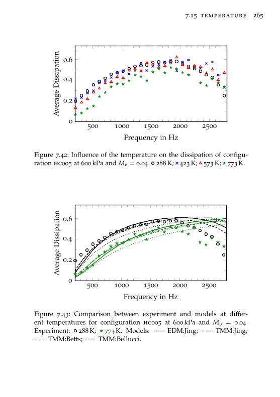
7.15 temperature 265
500 1000 1500 2000 25000
0.2
0.4
0.6
Frequency in Hz
Ave
rage
Dis
sipa
tion
Figure 7.42: Influence of the temperature on the dissipation of configu-ration hc005 at 600 kPa and Mb = 0.04. 288 K; 423 K; 573 K; 773 K.
500 1000 1500 2000 25000
0.2
0.4
0.6
Frequency in Hz
Ave
rage
Dis
sipa
tion
Figure 7.43: Comparison between experiment and models at differ-ent temperatures for configuration hc005 at 600 kPa and Mb = 0.04.Experiment: 288 K; 773 K. Models: EDM:Jing; TMM:Jing;
TMM:Betts; TMM:Bellucci.
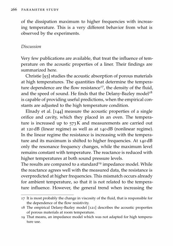
266 parameter study
of the dissipation maximum to higher frequencies with increas-ing temperature. This is a very different behavior from what isobserved by the experiments.
Discussion
Very few publications are available, that treat the influence of tem-perature on the acoustic properties of a liner. Their findings aresummarized here.
Christie [93] studies the acoustic absorption of porous materialsat high temperatures. The quantities that determine the tempera-ture dependence are the flow resistance17, the density of the fluid,and the speed of sound. He finds that the Delany-Bazley model18
is capable of providing useful predictions, when the empirical con-stants are adjusted to the high temperature condition.
Elnady et al. [144] measure the acoustic properties of a singleorifice and cavity, which they placed in an oven. The tempera-ture is increased up to 573 K and measurements are carried outat 120 dB (linear regime) as well as at 140 dB (nonlinear regime).In the linear regime the resistance is increasing with the tempera-ture and its maximum is shifted to higher frequencies. At 140 dBonly the resonance frequency changes, while the maximum levelremains constant with temperature. The reactance is reduced withhigher temperatures at both sound pressure levels.The results are compared to a standard19 impedance model. Whilethe reactance agrees well with the measured data, the resistance isoverpredicted at higher frequencies. This mismatch occurs alreadyfor ambient temperature, so that it is not related to the tempera-ture influence. However, the general trend when increasing the
17 It is most probably the change in viscosity of the fluid, that is responsible forthe dependence of the flow resistivity.
18 The empirical Delany-Bazley model [121] describes the acoustic propertiesof porous materials at room temperature.
19 That means, an impedance model which was not adapted for high tempera-ture use.
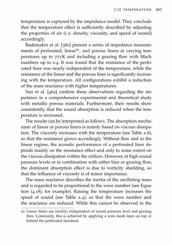
7.15 temperature 267
temperature is captured by the impedance model. They concludethat the temperature effect is sufficiently described by adjustingthe properties of air (i. e. density, viscosity, and speed of sound)accordingly.
Rademaker et al. [380] present a series of impedance measure-ments of perforated, linear20, and porous liners at varying tem-peratures up to 773 K and including a grazing flow with Machnumbers up to 0.4. It was found that the resistance of the perfo-rated liner was nearly independent of the temperature, while theresistance of the linear and the porous liner is significantly increas-ing with the temperature. All configurations exhibit a reductionof the mass reactance with higher temperatures.
Sun et al. [462] confirm these observations regarding the im-pedance in a comprehensive experimental and theoretical studywith metallic porous materials. Furthermore, their results showconsistently, that the sound absorption is reduced when the tem-perature is increased.
The results can be interpreted as follows. The absorption mecha-nism of linear or porous liners is mainly based on viscous dissipa-tion. The viscosity increases with the temperature (see Table a.6),so that the resistance grows accordingly. Without flow and in thelinear regime, the acoustic performance of a perforated liner de-pends mainly on the resonance effect and only to some extent onthe viscous dissipation within the orifices. However, at high soundpressure levels or in combination with either bias or grazing flow,the dominant absorption effect is due to vorticity shedding, sothat the influence of viscosity is of minor importance.
The mass reactance describes the inertia of the oscillating massand is regarded to be proportional to the wave number (see Equa-tion (4.18), for example). Raising the temperature increases thespeed of sound (see Table a.4), so that the wave number andthe reactance are reduced. While this cannot be observed in the
20 Linear liners are (nearly) independent of sound pressure level and grazingflow. Commonly, this is achieved by applying a wire mesh layer on top orbehind the perforated facesheet.
268 parameter study
data of Rademaker et al. [380] it will be mentioned here for com-pleteness, that the reactance is as well affected by the viscosity(see Equations (4.13) and (4.14)). The viscosity effect is commonlysmall compared to the wave number effect, but it counteracts theresults, i. e. the viscosity effect increases the reactance with thetemperature.
The results here present for the first time experimental data,which demonstrates the dependency of the absorption of a biasflow liner on the temperature. The main effect seems to be aslight reduction of the absorption with increasing temperature.This agrees with the results of Sun et al. [462] for a porous liner.However, the resonance frequency is not shifted to higher frequen-cies as reported in the literature, but remains unchanged.
A key difference between the references and the experimenthere is of course the bias flow. Additionally, the bias flow is notheated, but constantly at around 288 K, while the given temper-ature corresponds to the mean grazing flow temperature. Thisapproach with different bias and grazing flow temperatures re-flects the conditions at a combustor liner in a gas turbine, where,however, both temperatures are at a much higher level. Here, thetemperature within the cavity and the orifices of the liner is ratherconstant near its ambient value, which might be the reason for therather small influence of the temperature.
The temperature dependency observed in Figure 7.42 might beof an entirely different nature. Nayfeh and Sun [350] discusses theinfluence of a transverse temperature gradient on the absorptionof a liner. The effect can be compared to the refraction effect of asheared grazing flow (see the discussion in Section 7.3), with thedifference that it is independent of the direction of sound propaga-tion. Nayfeh and Sun [350] come to the conclusion that “[...] cool-ing the duct walls leads to channeling of the sound towards thewalls [...]”. Their theoretical experiment yields higher attenuationwhen the temperature of the wall is decreased, which contradictsthe findings here.
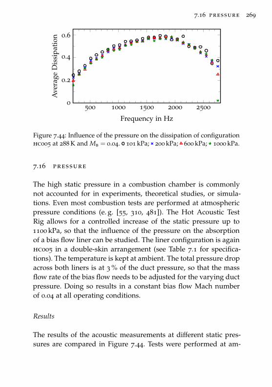
7.16 pressure 269
500 1000 1500 2000 25000
0.2
0.4
0.6
Frequency in Hz
Ave
rage
Dis
sipa
tion
Figure 7.44: Influence of the pressure on the dissipation of configurationhc005 at 288 K and Mb = 0.04. 101 kPa; 200 kPa; 600 kPa; 1000 kPa.
7.16 pressure
The high static pressure in a combustion chamber is commonlynot accounted for in experiments, theoretical studies, or simula-tions. Even most combustion tests are performed at atmosphericpressure conditions (e. g. [55, 310, 481]). The Hot Acoustic TestRig allows for a controlled increase of the static pressure up to1100 kPa, so that the influence of the pressure on the absorptionof a bias flow liner can be studied. The liner configuration is againhc005 in a double-skin arrangement (see Table 7.1 for specifica-tions). The temperature is kept at ambient. The total pressure dropacross both liners is at 3 % of the duct pressure, so that the massflow rate of the bias flow needs to be adjusted for the varying ductpressure. Doing so results in a constant bias flow Mach numberof 0.04 at all operating conditions.
Results
The results of the acoustic measurements at different static pres-sures are compared in Figure 7.44. Tests were performed at am-
270 parameter study
bient pressure (101 kPa), 200 kPa, 600 kPa, and 1000 kPa. The dis-sipation coefficient is largely unimpressed by the varying staticpressure. It seems that the static pressure does not change theacoustic properties of the liner.
The same result is predicted by the models. The predictionswithin the pressure range of the experiments are indistinguish-able, so that they are not shown here. The plot would reproducethe results at ambient conditions in Figure 7.43.
Discussion
The experimental results demonstrate, that the absorption of thebias flow liner is not at all depending on the static pressure (i. e.the density of the fluid, mainly).
Ahuja et al. [9] report about acoustic measurements of porousmaterials at sub-atmospheric pressures. It was observed that theabsorption of porous materials is decreasing when the pressure islowered.
In a theoretical study, Giese et al. [174] plot the maximum reach-able absorption coefficient and the corresponding flow resistanceof a porous ceramic tile at various pressures. The absorption coef-ficient remains constant while the flow resistance changes signifi-cantly. As a conclusion, the absorption is expected to change withthe pressure, when the flow resistance remains constant.
Judging from the references, the acoustic properties of porousmaterials are indeed depending on the pressure. However, theexperimental results with the bias flow liner paint a very clearpicture: The absorption due to the bias flow effect is independentof the operating pressure, i. e. it is insensitive to changes in thefluid density.
7.17 strouhal number 271
7.17 strouhal number
The Strouhal number21 is a dimensionless quantity relating thefrequency, a characteristic length, and the flow velocity. It is often-times used to describe the dependency of the acoustic propertiesof a bias flow liner on these quantities (e. g. [70, 210, 219, 242]).
Results
The experimental results of various frequencies and bias flow ve-locities is plotted over the Strouhal number in Figure 7.45. In theleft column the Strouhal number is based on the orifice radiusSt = kr/Mb, while it is based on the orifice length St = kl/Mb inthe right column. Mb is the mean bias flow Mach number in theorifice. Each row is a different liner configuration with varyingorifice radii and lengths.
Commonly, the Strouhal number is based on the orifice radius,as plotted in the left column. The Strouhal number where the dis-sipation is at maximum changes for the different configurations.This is indicated by the gray background. This variation is muchsmaller when the Strouhal number is based on the orifice length,as shown in the right column. Here, the maximum dissipation oc-curs in a smaller range of Strouhal numbers around unity, consis-tently for all configurations. In that case, it seems that the Strouhalnumber can be an indicator for maximum dissipation. However,the ’optimum’ Strouhal number alone does not grant an optimumdissipation. The levels of dissipation measured at Strouhal num-bers of unity for varying frequencies and bias flow velocities showa large diversity.
21 Named after Vincenc Strouhal (1850-1922, Czech physicist) [457].
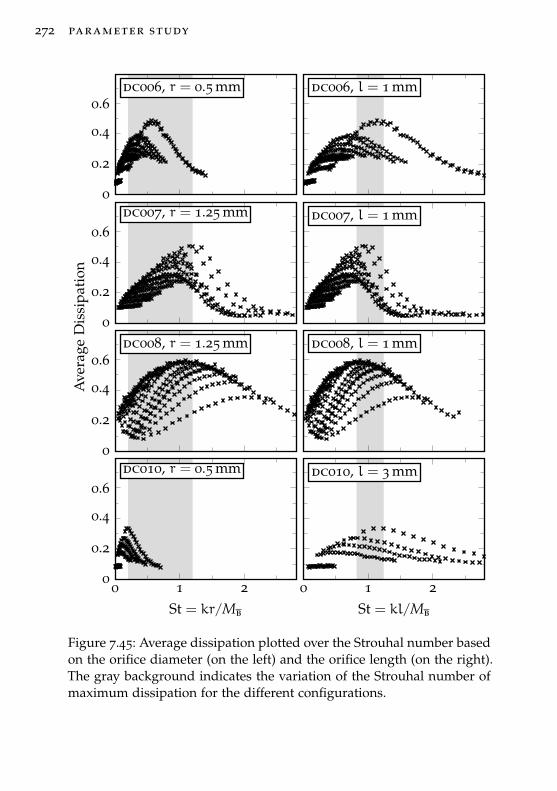
272 parameter study
dc006, r = 0.5 mm
0
0.2
0.4
0.6dc006, l = 1 mm
dc007, r = 1.25 mm
0
0.2
0.4
0.6dc007, l = 1 mm
dc008, r = 1.25 mm
0
0.2
0.4
0.6dc008, l = 1 mm
dc010, r = 0.5 mm
0 1 20
0.2
0.4
0.6
St = kr/Mb
dc010, l = 3 mm
0 1 2St = kl/Mb
Ave
rage
Dis
sipa
tion
Figure 7.45: Average dissipation plotted over the Strouhal number basedon the orifice diameter (on the left) and the orifice length (on the right).The gray background indicates the variation of the Strouhal number ofmaximum dissipation for the different configurations.
7.17 strouhal number 273
Discussion
Bodén and Zhou [70] successfully collapse their experimental datawhen expressing it in terms of Rayleigh conductivity and plot-ting it over the inverse Strouhal number. This confirms Howe’sapproach of using the Strouhal number as the only parameterin his model of the Rayleigh conductivity. Unfortunately, the dis-sipation coefficient does not have a unique relationship to theStrouhal number. However, maximum absorption can be achievedfor Strouhal numbers of unity, when the Strouhal number is basedon the orifice length rather than the orifice radius.

8C O N C L U D I N G R E M A R K S
This thesis provides a comprehensive experimental parameter stu-dy of bias flow liners regarding their geometric, thermodynamic,acoustic, and flow parameters. An extensive amount of availableresearch has been collected and reviewed. The consistent databaseof experimental results allowed to put the existing informationinto perspective. The significant features of each parameter canbe summarized as follows:
sound pressure level The behavior of the liner is linearwhen the bias flow velocity is larger than the acoustic velocity,that is when flow reversal does not occur. A combustor liner isrequired to operate in the linear regime to prevent hot gas inges-tion.
bias flow The bias flow was able to improve the absorptionof all tested configuration, compared to the acoustic performancewithout flow. Two scenarios can be distinguished: The bias flowacting on the resonance effect and the pure bias flow effect. Inthe first case, the bias flow shifts the frequency of maximum dis-sipation to higher values. The bandwidth of the absorption is in-creased while its level is typically reduced. True broadband ab-sorption is obtained when the bias flow effect dominates.
276 concluding remarks
grazing flow The effect of the grazing flow on the acousticproperties of a perforated liner is identical to the bias flow effect.In order to achieve similar results the mean grazing flow Machnumber must be a factor of ≈ 3.5 higher than the Mach numberof the bias flow jets. However, at certain combinations of graz-ing flow velocities and liner geometries sound might be producedrather than absorbed. Due to the convective effect of the grazingflow, the absorption of sound waves traveling against flow direc-tion is increased while it is reduced in the opposite direction.
simultaneous grazing & bias flow The influence of thegrazing flow can be neglected when the ratio of bias to grazingflow velocity is larger than Mb/Mg > 0.3. This corresponds to thecondition Mg ≈ 3.5 Mb, where a similar dissipation is obtainedwhen bias or grazing flows are applied separately. Below this limitthe influence of the grazing flow can be accounted for by an effec-tive discharge coefficient, which essentially increases the bias flowvelocity.
porosity When the bias flow effect dominates the magnitudeof the dissipation is directly related to the level of porosity. Theindividual parameters orifice area, orifice spacing, and number oforifices are unimportant. The situation is more complex withoutbias flow and in the transition region between resonance regimeand bias flow regime.
wall thickness The wall thickness seems to be of minor sig-nificance at high bias flow velocities. A thin configuration is su-perior, in particular concerning the bandwidth, at low bias flowvelocities.
orifice cross-section shape The acoustic performance islargely independent of the orifice cross-section shape, when the
concluding remarks 277
open area remains constant. However, an effect is expected forlong and narrow openings.
orifice edge geometry The velocity of the bias flow jet isvery sensitive to the orifice edge geometry. The experimental datareveals that it is indeed the jet velocity and not the orifice meanvelocity, which needs to be constant when comparing different se-tups. Complying with this rule, the orifice edge geometry exhibitsonly a minor influence on the absorption. The observed behaviormight be the result of the effectively reduced length and the in-creased open area at the surface when both edges are rounded.
orifice angle The average dissipation is independent of theorifice angle at high bias flow velocities. At lower velocities moreshallow angles result in a slightly superior bandwidth. The ab-sorption of sound waves traveling in direction of the bias flowinjection is increased, while it is reduced in the other direction.For a typical installation that counteracts the convective effect ofa grazing flow.
double-skin configuration A double-skin configurationallows for a reduction of the bias flow velocity through the damp-ing liner when a certain pressure drop needs to be met. The in-fluence of the second liner on the acoustic performance becomesinsignificant when the bias flow velocity increases.
cavity volume In the resonance dominated regime, the fre-quency of maximum dissipation is associated with the Hemholtzresonance, which is inversely proportional to the cavity volume.Introducing a bias flow shifts the dissipation maximum to higherfrequencies. In the bias flow regime the no flow Helmholtz res-onance frequency provides a cut-off frequency, below which theabsorption falls off from its broadband maximum level.
278 concluding remarks
partitioned cavity Dividing the cavity into several smallercavities while keeping their Helmholtz resonance constant, ampli-fies the resonance effect. However, the partitions show no influ-ence when the bias flow velocity is high.
perforation placement The placement of the perforationrelative to the liner cavity becomes important when the cavity islonger than half an acoustic wave length. In that case, it shouldbe preferred to place the perforation only at the pressure nodesof the axial resonance in the cavity. The experiments show that aconfiguration with alternating areas of hard-wall and perforationyields an improved absorption.
perforation pattern The absorption seems largely inde-pendent of the perforation pattern. However, a nonuniform cir-cumferential perforation distribution can be used to promote acircumferential resonance.
temperature Increasing the temperature of the grazing flowresults in a reduction of the absorption. However, in this setupthe bias flow is not heated, so that this result reflects the influenceof the temperature difference between grazing and bias flow, asexperienced in a combustor.
pressure The pressure seems to have no influence on the ab-sorption.
strouhal number Maximum dissipation can be obtained ata Strouhal number of unity, when the Strouhal number is basedon the orifice length rather than the orifice radius. However, aStrouhal number of unity seems to be a neccessary condition only,but is not sufficient that maximum absorption will be achieved.
concluding remarks 279
Many of the parameters are becoming insignificant when thebias flow effect dominates. There seems to be a fundamentally dif-ferent behavior of bias flow liners at low velocities, depending onthe resonance characteristics of the liner-cavity system. If a reso-nance occurs without flow, then the bias flow shifts the absorptionmaximum to higher frequencies and broadens its frequency range.Ultimately, the bias flow suppresses the resonance effect leadingto a broadband absorption, typically at a much lower level thenthe maximum observed due to the resonance effect. In the casewithout resonance, the acoustic performance of the liner is verypoor without bias flow. The bias flow continuously increases theabsorption until an optimum is reached, where the acoustic per-formance surpasses the best achievement of a resonance type linerin absorption level and frequency range. Bias flow velocities suc-ceeding this optimum increase the broadband damping towardshigher frequencies, while it reduces the level of the broadbandabsorption. The condition that decides which behavior will occur,i. e. if a resonance is provoked or suppressed, is not clear. Here,it seems to correlate with the porosity of the liner. The resonanceeffect occurs at low porosities (here around 1 %) and is absent athigh porosities (here > 6.8 %).
The domination of the bias flow effect on the acoustic dampingperformance is mainly determined by three parameters: the biasflow velocity, the porosity, and the no flow Helmholtz resonancefrequency of the liner-cavity system (assuming all dimensions aremuch smaller than the wave length). The Helmholtz resonancefrequency is determined by the combination of the porosity, thewall thickness, and the cavity volume. It provides a cut-off fre-quency, below which the absorption falls off from its broadbandmaximum level (see Figure 7.33). The upper frequency limit of thebroadband absorption is pushed to higher values while the biasflow velocity is increased, however, at the penalty of lowering theabsorption level. The level of the broadband absorption is depend-

280 concluding remarks
ing on the porosity and bias flow velocity. Higher porosities yieldan improved absorption when keeping the velocity constant.
Models
All models capture the general trends of the experiments fairlywell. It is quite surprising that the deviation between the modelsthemselves is rather small, considering the different approachestaken. The agreement between the models and the experimentaldata is generally satisfactory. However, all models tend to under-estimate the dissipation. The best agreement is achieved wherethe bias flow effect is described by Howe’s theory, i. e. by Jing andBellucci. While the Bellucci model has been extended to functionas well when there is no bias flow, the Jing model is restricted tothe presence of a bias flow.
The Eldredge and Dowling method (EDM) and the transfer ma-trix method (TMM) give largely similar results, while EDM pre-dicts slightly higher dissipation values, which often reproducesthe experimental results a bit better. Both methods have someunique features readily available. EDM provides the ability to in-clude a second liner in a double-skin configuration. TMM allowsfor the simple integration of hard-wall extensions on both sides ofthe perforation, in the case where the perforation does not coverthe entire length of the cavity.
One common problem of the models is the transition betweenthe resonance dominated damping to the purely bias flow relatedregime. This transition seems to be mainly governed by the reduc-tion of the reactance. While there is a wide variety in the modelsof the behavior of the reactance, none seems to capture it quiteright. Recent numerical models by Jing and Sun [242] and Leeet al. [291] predict a much stronger effect on the reactance.
concluding remarks 281
Outlook
The models and conclusions that have been drawn here and else-where are often based purely on empiricism. An enhanced phys-ical understanding of the underlying mechanisms is needed toimprove the prediction quality of the models. Recent studies byRupp and Carrotte [415] and Heuwinkel et al. [201] and the ongo-ing work of Schulz et al. [436] point into this direction. They alluse optical measurement techniques to capture the physical effectright at the orifice. The results of further efforts in this directionare highly anticipated.

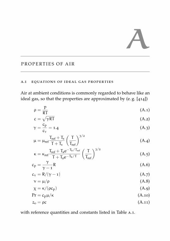
AP R O P E RT I E S O F A I R
a.1 equations of ideal gas properties
Air at ambient conditions is commonly regarded to behave like anideal gas, so that the properties are approximated by (e. g. [414])
ρ =p
RT(A.1)
c =√γRT (A.2)
γ =cp
cv= 1.4 (A.3)
µ = µrefTref + Ts
T + Ts
(T
Tref
)3/2
(A.4)
κ = κrefTref + Tae−Tb/Tref
T + Tae−Tb/T
(T
Tref
)3/2
(A.5)
cp =γ
γ− 1R (A.6)
cv = R/(γ− 1) (A.7)
ν = µ/ρ (A.8)
χ = κ/(ρcp) (A.9)
Pr = cpµ/κ (A.10)
z0 = ρc (A.11)
with reference quantities and constants listed in Table a.1.
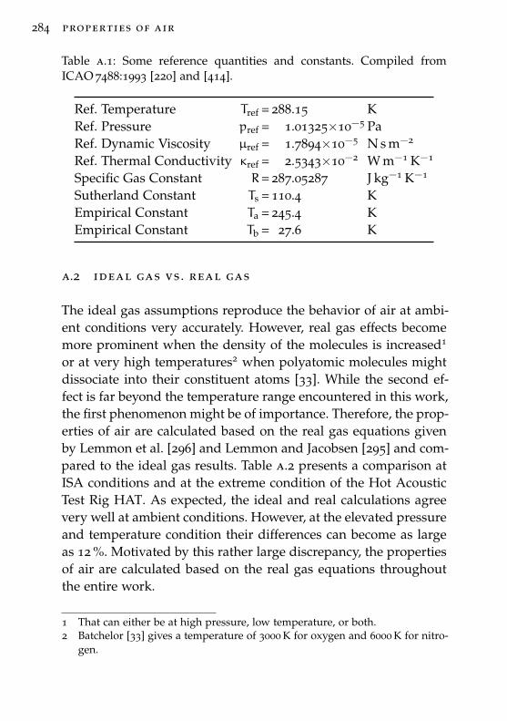
284 properties of air
Table a.1: Some reference quantities and constants. Compiled fromICAO 7488:1993 [220] and [414].
Ref. Temperature Tref = 288.15 KRef. Pressure pref = 1.01325×10⁻⁵ PaRef. Dynamic Viscosity µref = 1.7894×10⁻⁵ N s m−2
Ref. Thermal Conductivity κref = 2.5343×10⁻² W m−1 K−1
Specific Gas Constant R= 287.05287 J kg−1 K−1
Sutherland Constant Ts = 110.4 KEmpirical Constant Ta = 245.4 KEmpirical Constant Tb = 27.6 K
a.2 ideal gas vs . real gas
The ideal gas assumptions reproduce the behavior of air at ambi-ent conditions very accurately. However, real gas effects becomemore prominent when the density of the molecules is increased1
or at very high temperatures2 when polyatomic molecules mightdissociate into their constituent atoms [33]. While the second ef-fect is far beyond the temperature range encountered in this work,the first phenomenon might be of importance. Therefore, the prop-erties of air are calculated based on the real gas equations givenby Lemmon et al. [296] and Lemmon and Jacobsen [295] and com-pared to the ideal gas results. Table a.2 presents a comparison atISA conditions and at the extreme condition of the Hot AcousticTest Rig HAT. As expected, the ideal and real calculations agreevery well at ambient conditions. However, at the elevated pressureand temperature condition their differences can become as largeas 12 %. Motivated by this rather large discrepancy, the propertiesof air are calculated based on the real gas equations throughoutthe entire work.
1 That can either be at high pressure, low temperature, or both.2 Batchelor [33] gives a temperature of 3000 K for oxygen and 6000 K for nitro-
gen.
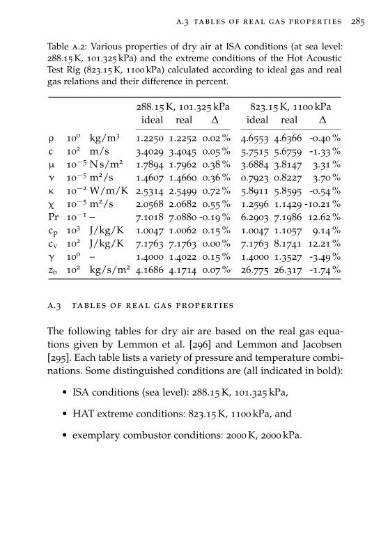
a.3 tables of real gas properties 285
Table a.2: Various properties of dry air at ISA conditions (at sea level:288.15 K, 101.325 kPa) and the extreme conditions of the Hot AcousticTest Rig (823.15 K, 1100 kPa) calculated according to ideal gas and realgas relations and their difference in percent.
288.15 K, 101.325 kPa 823.15 K, 1100 kPaideal real ∆ ideal real ∆
ρ 100 kg/m3 1.2250 1.2252 0.02 % 4.6553 4.6366 -0.40 %c 102 m/s 3.4029 3.4045 0.05 % 5.7515 5.6759 -1.33 %µ 10−5 N s/m2 1.7894 1.7962 0.38 % 3.6884 3.8147 3.31 %ν 10−5 m2/s 1.4607 1.4660 0.36 % 0.7923 0.8227 3.70 %κ 10−2 W/m/K 2.5314 2.5499 0.72 % 5.8911 5.8595 -0.54 %χ 10−5 m2/s 2.0568 2.0682 0.55 % 1.2596 1.1429 -10.21 %Pr 10−1 – 7.1018 7.0880 -0.19 % 6.2903 7.1986 12.62 %cp 103 J/kg/K 1.0047 1.0062 0.15 % 1.0047 1.1057 9.14 %cv 102 J/kg/K 7.1763 7.1763 0.00 % 7.1763 8.1741 12.21 %γ 100 – 1.4000 1.4022 0.15 % 1.4000 1.3527 -3.49 %z0 102 kg/s/m2 4.1686 4.1714 0.07 % 26.775 26.317 -1.74 %
a.3 tables of real gas properties
The following tables for dry air are based on the real gas equa-tions given by Lemmon et al. [296] and Lemmon and Jacobsen[295]. Each table lists a variety of pressure and temperature combi-nations. Some distinguished conditions are (all indicated in bold):
• ISA conditions (sea level): 288.15 K, 101.325 kPa,
• HAT extreme conditions: 823.15 K, 1100 kPa, and
• exemplary combustor conditions: 2000 K, 2000 kPa.
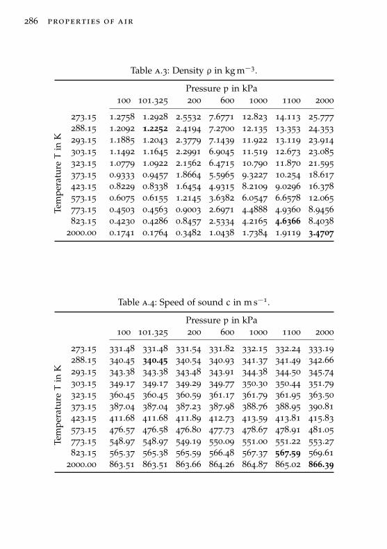
286 properties of air
Table a.3: Density ρ in kg m−3.
Pressure p in kPa100 101.325 200 600 1000 1100 2000
Tem
pera
tureT
inK
273.15 1.2758 1.2928 2.5532 7.6771 12.823 14.113 25.777288.15 1.2092 1.2252 2.4194 7.2700 12.135 13.353 24.353293.15 1.1885 1.2043 2.3779 7.1439 11.922 13.119 23.914303.15 1.1492 1.1645 2.2991 6.9045 11.519 12.673 23.085323.15 1.0779 1.0922 2.1562 6.4715 10.790 11.870 21.595373.15 0.9333 0.9457 1.8664 5.5965 9.3227 10.254 18.617423.15 0.8229 0.8338 1.6454 4.9315 8.2109 9.0296 16.378573.15 0.6075 0.6155 1.2145 3.6382 6.0547 6.6578 12.065773.15 0.4503 0.4563 0.9003 2.6971 4.4888 4.9360 8.9456823.15 0.4230 0.4286 0.8457 2.5334 4.2165 4.6366 8.4038
2000.00 0.1741 0.1764 0.3482 1.0438 1.7384 1.9119 3.4707
Table a.4: Speed of sound c in m s−1.
Pressure p in kPa100 101.325 200 600 1000 1100 2000
T em
pera
tureT
inK
273.15 331.48 331.48 331.54 331.82 332.15 332.24 333.19288.15 340.45 340.45 340.54 340.93 341.37 341.49 342.66293.15 343.38 343.38 343.48 343.91 344.38 344.50 345.74303.15 349.17 349.17 349.29 349.77 350.30 350.44 351.79323.15 360.45 360.45 360.59 361.17 361.79 361.95 363.50373.15 387.04 387.04 387.23 387.98 388.76 388.95 390.81423.15 411.68 411.68 411.89 412.73 413.59 413.81 415.83573.15 476.57 476.58 476.80 477.73 478.67 478.91 481.05773.15 548.97 548.97 549.19 550.09 551.00 551.22 553.27823.15 565.37 565.38 565.59 566.48 567.37 567.59 569.61
2000.00 863.51 863.51 863.66 864.26 864.87 865.02 866.39
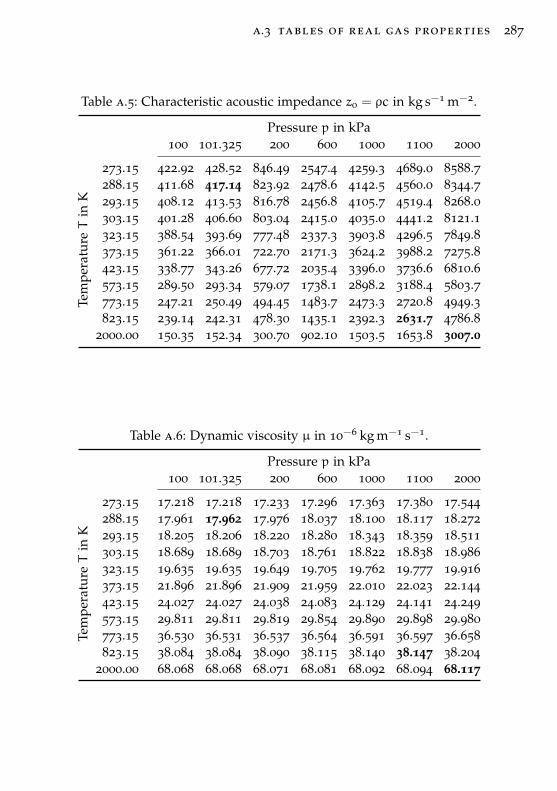
a.3 tables of real gas properties 287
Table a.5: Characteristic acoustic impedance z0 = ρc in kg s−1 m−2.
Pressure p in kPa100 101.325 200 600 1000 1100 2000
T em
pera
tureT
inK
273.15 422.92 428.52 846.49 2547.4 4259.3 4689.0 8588.7288.15 411.68 417.14 823.92 2478.6 4142.5 4560.0 8344.7293.15 408.12 413.53 816.78 2456.8 4105.7 4519.4 8268.0303.15 401.28 406.60 803.04 2415.0 4035.0 4441.2 8121.1323.15 388.54 393.69 777.48 2337.3 3903.8 4296.5 7849.8373.15 361.22 366.01 722.70 2171.3 3624.2 3988.2 7275.8423.15 338.77 343.26 677.72 2035.4 3396.0 3736.6 6810.6573.15 289.50 293.34 579.07 1738.1 2898.2 3188.4 5803.7773.15 247.21 250.49 494.45 1483.7 2473.3 2720.8 4949.3823.15 239.14 242.31 478.30 1435.1 2392.3 2631.7 4786.8
2000.00 150.35 152.34 300.70 902.10 1503.5 1653.8 3007.0
Table a.6: Dynamic viscosity µ in 10−6 kg m−1 s−1.
Pressure p in kPa100 101.325 200 600 1000 1100 2000
Tem
pera
tureT
inK
273.15 17.218 17.218 17.233 17.296 17.363 17.380 17.544288.15 17.961 17.962 17.976 18.037 18.100 18.117 18.272293.15 18.205 18.206 18.220 18.280 18.343 18.359 18.511303.15 18.689 18.689 18.703 18.761 18.822 18.838 18.986323.15 19.635 19.635 19.649 19.705 19.762 19.777 19.916373.15 21.896 21.896 21.909 21.959 22.010 22.023 22.144423.15 24.027 24.027 24.038 24.083 24.129 24.141 24.249573.15 29.811 29.811 29.819 29.854 29.890 29.898 29.980773.15 36.530 36.531 36.537 36.564 36.591 36.597 36.658823.15 38.084 38.084 38.090 38.115 38.140 38.147 38.204
2000.00 68.068 68.068 68.071 68.081 68.092 68.094 68.117
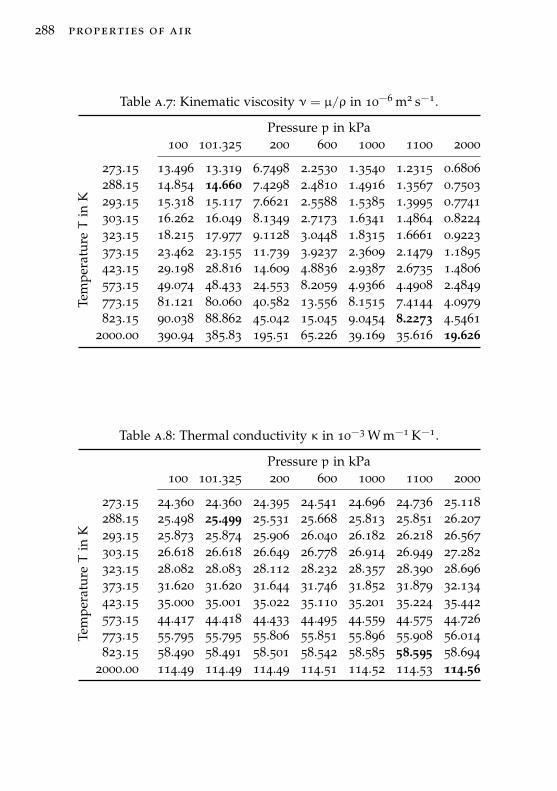
288 properties of air
Table a.7: Kinematic viscosity ν = µ/ρ in 10−6 m2 s−1.
Pressure p in kPa100 101.325 200 600 1000 1100 2000
T em
pera
tureT
inK
273.15 13.496 13.319 6.7498 2.2530 1.3540 1.2315 0.6806288.15 14.854 14.660 7.4298 2.4810 1.4916 1.3567 0.7503293.15 15.318 15.117 7.6621 2.5588 1.5385 1.3995 0.7741303.15 16.262 16.049 8.1349 2.7173 1.6341 1.4864 0.8224323.15 18.215 17.977 9.1128 3.0448 1.8315 1.6661 0.9223373.15 23.462 23.155 11.739 3.9237 2.3609 2.1479 1.1895423.15 29.198 28.816 14.609 4.8836 2.9387 2.6735 1.4806573.15 49.074 48.433 24.553 8.2059 4.9366 4.4908 2.4849773.15 81.121 80.060 40.582 13.556 8.1515 7.4144 4.0979823.15 90.038 88.862 45.042 15.045 9.0454 8.2273 4.5461
2000.00 390.94 385.83 195.51 65.226 39.169 35.616 19.626
Table a.8: Thermal conductivity κ in 10−3 W m−1 K−1.
Pressure p in kPa100 101.325 200 600 1000 1100 2000
Tem
pera
tureT
inK
273.15 24.360 24.360 24.395 24.541 24.696 24.736 25.118288.15 25.498 25.499 25.531 25.668 25.813 25.851 26.207293.15 25.873 25.874 25.906 26.040 26.182 26.218 26.567303.15 26.618 26.618 26.649 26.778 26.914 26.949 27.282323.15 28.082 28.083 28.112 28.232 28.357 28.390 28.696373.15 31.620 31.620 31.644 31.746 31.852 31.879 32.134423.15 35.000 35.001 35.022 35.110 35.201 35.224 35.442573.15 44.417 44.418 44.433 44.495 44.559 44.575 44.726773.15 55.795 55.795 55.806 55.851 55.896 55.908 56.014823.15 58.490 58.491 58.501 58.542 58.585 58.595 58.694
2000.00 114.49 114.49 114.49 114.51 114.52 114.53 114.56
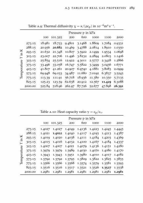
a.3 tables of real gas properties 289
Table a.9: Thermal diffusivity χ = κ/(ρcp) in 10−6m2 s−1.
Pressure p in kPa100 101.325 200 600 1000 1100 2000
T em
pera
tureT
inK
273.15 18.981 18.733 9.4801 3.1468 1.8809 1.7084 0.9331288.15 20.956 20.682 10.469 3.4788 2.0814 1.8910 1.0350293.15 21.632 21.348 10.807 3.5922 2.1499 1.9534 1.0698303.15 23.007 22.706 11.496 3.8232 2.2894 2.0803 1.1406323.15 25.854 25.516 12.922 4.3011 2.5777 2.3428 1.2866373.15 33.496 33.058 16.747 5.5822 3.3499 3.0456 1.6771423.15 41.807 41.261 20.907 6.9740 4.1881 3.8083 2.0999573.15 69.948 69.033 34.987 11.680 7.0192 6.3837 3.5245773.15 113.39 111.91 56.718 18.936 11.380 10.350 5.7135823.15 125.23 123.59 62.638 20.912 12.567 11.429 6.3088
2000.00 525.84 518.96 262.97 87.726 52.677 47.898 26.391
Table a.10: Heat capacity ratio γ = cp/cv.
Pressure p in kPa100 101.325 200 600 1000 1100 2000
Tem
pera
tureT
inK
273.15 1.4027 1.4027 1.4049 1.4136 1.4223 1.4245 1.4445288.15 1.4021 1.4022 1.4040 1.4117 1.4193 1.4213 1.4387293.15 1.4019 1.4020 1.4038 1.4111 1.4184 1.4203 1.4369303.15 1.4015 1.4016 1.4032 1.4100 1.4167 1.4184 1.4337323.15 1.4007 1.4007 1.4021 1.4079 1.4136 1.4151 1.4280373.15 1.3979 1.3979 1.3989 1.4030 1.4070 1.4080 1.4170423.15 1.3943 1.3943 1.3951 1.3980 1.4010 1.4017 1.4082573.15 1.3792 1.3792 1.3795 1.3809 1.3822 1.3825 1.3855773.15 1.3566 1.3566 1.3568 1.3574 1.3579 1.3581 1.3593823.15 1.3516 1.3516 1.3517 1.3521 1.3526 1.3527 1.3538
2000.00 1.2981 1.2981 1.2981 1.2981 1.2981 1.2981 1.2981
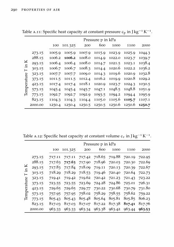
290 properties of air
Table a.11: Specific heat capacity at constant pressure cp in J kg−1 K−1.
Pressure p in kPa100 101.325 200 600 1000 1100 2000
Tem
pera
tureT
inK
273.15 1005.9 1005.9 1007.9 1015.9 1023.9 1025.9 1044.3288.15 1006.2 1006.2 1008.0 1014.9 1022.0 1023.7 1039.7293.15 1006.4 1006.4 1008.0 1014.7 1021.5 1023.1 1038.4303.15 1006.7 1006.7 1008.3 1014.4 1020.6 1022.2 1036.2323.15 1007.7 1007.7 1009.0 1014.3 1019.6 1020.9 1032.8373.15 1011.5 1011.5 1012.4 1016.2 1019.9 1020.8 1029.2423.15 1017.4 1017.4 1018.1 1020.9 1023.7 1024.3 1030.5573.15 1045.4 1045.4 1045.7 1047.1 1048.5 1048.8 1051.9773.15 1092.7 1092.7 1092.9 1093.5 1094.2 1094.4 1095.9823.15 1104.3 1104.3 1104.4 1105.0 1105.6 1105.7 1107.1
2000.00 1250.4 1250.4 1250.5 1250.5 1250.6 1250.6 1250.7
Table a.12: Specific heat capacity at constant volume cv in J kg−1 K−1.
Pressure p in kPa100 101.325 200 600 1000 1100 2000
T em
pera
tureT
inK
273.15 717.11 717.11 717.42 718.65 719.88 720.19 722.95288.15 717.63 717.63 717.90 718.96 720.03 720.30 722.69293.15 717.83 717.84 718.09 719.11 720.13 720.39 722.67303.15 718.29 718.29 718.53 719.46 720.40 720.64 722.73323.15 719.41 719.42 719.62 720.42 721.23 721.43 723.22373.15 723.55 723.55 723.69 724.28 724.86 725.01 726.31423.15 729.65 729.65 729.77 730.22 730.68 730.79 731.80573.15 757.95 757.95 758.02 758.29 758.55 758.62 759.22773.15 805.43 805.43 805.48 805.64 805.81 805.85 806.23823.15 817.03 817.03 817.07 817.22 817.38 817.41 817.76
2000.00 963.33 963.33 963.34 963.38 963.42 963.44 963.53
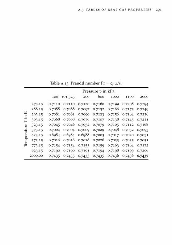
a.3 tables of real gas properties 291
Table a.13: Prandtl number Pr = cpµ/κ.
Pressure p in kPa100 101.325 200 600 1000 1100 2000
Tem
pera
tureT
inK
273.15 0.7110 0.7110 0.7120 0.7160 0.7199 0.7208 0.7294288.15 0.7088 0.7088 0.7097 0.7132 0.7166 0.7175 0.7249293.15 0.7081 0.7081 0.7090 0.7123 0.7156 0.7164 0.7236303.15 0.7068 0.7068 0.7076 0.7107 0.7138 0.7145 0.7211323.15 0.7045 0.7046 0.7052 0.7079 0.7105 0.7112 0.7168373.15 0.7004 0.7004 0.7009 0.7029 0.7048 0.7052 0.7093423.15 0.6984 0.6984 0.6988 0.7003 0.7017 0.7020 0.7051573.15 0.7016 0.7016 0.7018 0.7026 0.7033 0.7035 0.7051773.15 0.7154 0.7154 0.7155 0.7159 0.7163 0.7164 0.7172823.15 0.7190 0.7190 0.7191 0.7194 0.7198 0.7199 0.7206
2000.00 0.7435 0.7435 0.7435 0.7435 0.7436 0.7436 0.7437

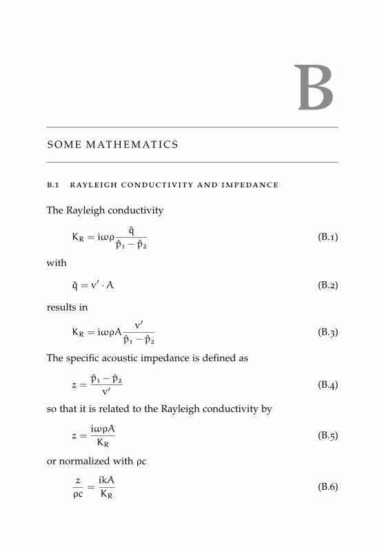
BS O M E M AT H E M AT I C S
b.1 rayleigh conductivity and impedance
The Rayleigh conductivity
KR = iωρq
p1 − p2(B.1)
with
q = v′ ·A (B.2)
results in
KR = iωρAv′
p1 − p2(B.3)
The specific acoustic impedance is defined as
z =p1 − p2
v′(B.4)
so that it is related to the Rayleigh conductivity by
z =iωρAKR
(B.5)
or normalized with ρc
z
ρc=
ikAKR
(B.6)
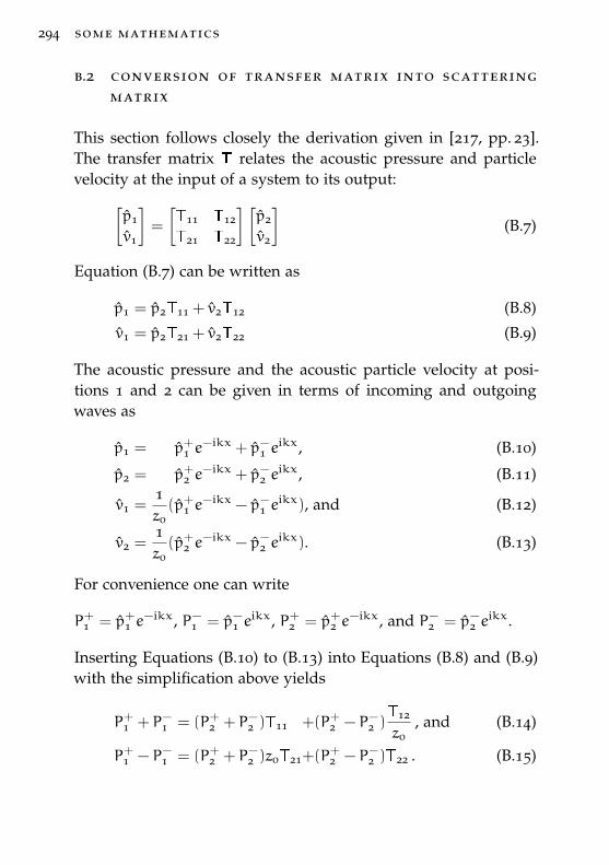
294 some mathematics
b.2 conversion of transfer matrix into scatteringmatrix
This section follows closely the derivation given in [217, pp. 23].The transfer matrix T relates the acoustic pressure and particlevelocity at the input of a system to its output:[
p1
v1
]=
[T11 T12
T21 T22
] [p2
v2
](B.7)
Equation (B.7) can be written as
p1 = p2T11 + v2T12 (B.8)
v1 = p2T21 + v2T22 (B.9)
The acoustic pressure and the acoustic particle velocity at posi-tions 1 and 2 can be given in terms of incoming and outgoingwaves as
p1 = p+1 e−ikx + p−1 e
ikx, (B.10)
p2 = p+2 e−ikx + p−2 e
ikx, (B.11)
v1 =1z0(p+1 e
−ikx − p−1 eikx), and (B.12)
v2 =1z0(p+2 e
−ikx − p−2 eikx). (B.13)
For convenience one can write
P+1 = p+1 e−ikx, P−1 = p−1 e
ikx, P+2 = p+2 e−ikx, and P−2 = p−2 e
ikx.
Inserting Equations (B.10) to (B.13) into Equations (B.8) and (B.9)with the simplification above yields
P+1 + P−1 = (P+2 + P−2 )T11 +(P+2 − P−2 )T12
z0, and (B.14)
P+1 − P−1 = (P+2 + P−2 )z0T21+(P+2 − P−2 )T22 . (B.15)
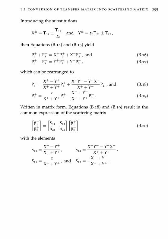
b.2 conversion of transfer matrix into scattering matrix 295
Introducing the substitutions
X± = T11 ±T12
z0and Y± = z0T21 ±T22 ,
then Equations (B.14) and (B.15) yield
P+1 + P−1 = X+P+2 +X−P−2 , and (B.16)
P+1 − P−1 = Y+P+2 + Y−P−2 , (B.17)
which can be rearranged to
P−1 =X+ − Y+
X+ + Y+P+1 +
X+Y− − Y+X−
X+ + Y−P−2 , and (B.18)
P+2 =2
X+ + Y+P+1 −
X− + Y−
X+ + Y+P−2 . (B.19)
Written in matrix form, Equations (B.18) and (B.19) result in thecommon expression of the scattering matrix[
p−1p+2
]=
[S11 S12
S21 S22
] [p+1p−2
](B.20)
with the elements
S11 =X+ − Y+
X+ + Y+, S12 =
X+Y− − Y+X−
X+ + Y+,
S21 =2
X+ + Y+, and S22 = −
X− + Y−
X+ + Y+.

B I B L I O G R A P H Y
[1] Åbom, M.: “Measurement of the scattering-matrix of acoustical two-ports”, Mechanical Systems and Signal Processing, 5(2):89–104, 1991. (Citedon pages 139, 153, and 154.)
[2] Åbom, M.; Bodén, H.: “Error analysis of two-microphone measurementsin ducts with flow”, Journal of the Acoustical Society of America, 83(6):2429–2438, 1988. (Cited on pages 146 and 147.)
[3] Abramowitz, M.; Stegun, I.A.: Handbook of mathematical functions, Ap-plied Mathematics Series 55, National Bureau of Standards, 1970. (Citedon pages 62 and 103.)
[4] ACARE: “European aeronautics: A vision for 2020”, Report, AdvisoryCouncil for Aviation Research and Innovation in Europe, 2001. (Citedon page 4.)
[5] ACARE: “Flightpath 2050 - Europe’s vision for aviation”, Report, Advi-sory Council for Aviation Research and Innovation in Europe, 2011. (Citedon page 4.)
[6] Ahuja, K.K.; Cataldi, P.; R. J. Gaeta, J.: “Sound absorption of a 2DOF res-onant liner with negative bias flow”, Contractor Report NASA-CR-2000-210637, NASA, 2000. (Cited on pages 34 and 54.)
[7] Ahuja, K.K.; Gaeta, R.J.: “Active control of liner impedance by varyingperforate orifice geometry”, Contractor Report NASA-CR-2000-210633,NASA, 2000. (Cited on pages 17, 28, 38, and 235.)
[8] Ahuja, K.K.; Gaeta, R.J.; Agostino, M.D.: “Acoustic absorption charac-teristics of an orifice with a mean bias flow”, Contractor Report NASA-CR-2000-210636, NASA, 2000. (Cited on pages 28, 29, 35, and 54.)
[9] Ahuja, K.K.; Gaeta, R.J.; Hsu, J.S.: “Acoustic properties and durabilitiyof liner materials at non-standard atmospheric conditions”, ContractorReport NASA-CR-195010, NASA, 1994. (Cited on pages 26 and 270.)
[10] Ahuja, K.K.; R. J. Gaeta, J.; D’Agostino, M.: “High amplitude acousticbehaviour of a slit-orifice backed by a cavity”, Contractor Report NASA-CR-2000-210635, NASA, 2000. (Cited on page 18.)
298 bibliography
[11] Alfredson, R.J.; Davies, P.O.A.L.: “Performance of exhaust silencer com-ponents”, Journal of Sound and Vibration, 15(2):175–196, 1971. (Cited onpage 53.)
[12] Allam, S.; Åbom, M.: “Acoustic modelling and testing of a complex carmuffler”, in International Congress on Sound and Vibration, ICSV13, 2-6 July2006, Vienna, Austria, 2006. (Cited on page 73.)
[13] Allam, S.; Åbom, M.: “Investigation of damping and radiation usingfull plane wave decomposition in ducts”, Journal of Sound and Vibration,292:519–534, 2006. (Cited on pages 124 and 126.)
[14] Allam, S.; Åbom, M.: “Experimental characterization of acoustic linerswith extended reaction”, in 14th AIAA/CEAS Aeroacoustics Conference, 5-7May 2008, Vancouver, Canada, AIAA-2008-3074, 2008. (Cited on pages 45,73, and 75.)
[15] Anderson, J.D.: “Ludwig Prandtl’s boundary layer”, Physics Today,58(1):42–48, 2005. (Cited on page 117.)
[16] Andreini, A.; Bianchini, C.; Facchini, B.; Simonetti, F.; Peschiulli,A.: “Assessment of numerical tools for the evaluation of the acousticimpedance of multi-perforated plates”, in ASME Turbo Expo 2011, 6-10June 2011, Vancouver, Canada, GT2011-46303, 2011. (Cited on pages 16, 19,47, 49, 55, and 71.)
[17] Andreini, A.; Facchini, B.; Ferrari, L.; Lenzi, G.; Simonetti, F.;A.Peschiulli: “Experimental investigation of effusion liner geometriesfor aero-engine combustors: Evaluation of global acoustic parameters”,in ASME Turbo Expo 2012, 11-15 June 2012, Copenhagen, Denmark, GT2012-69853, 2012. (Cited on pages 16, 19, 22, 35, 49, 50, 55, 72, 139, 245, 246, 262,and 263.)
[18] Andreini, A.; Facchini, B.; Giusti, A.; Vitale, I.; Turrini, F.: “Thermoa-coustic analysis of a full annular lean burn aero-engine combustor”, inASME Turbo Expo 2013, 3-7 June 2013, San Antonio, Texas, USA, GT2013-94877, 2013. (Cited on pages 45, 49, 55, 73, and 75.)
[19] Andreini, A.; Facchini, B.; Picchi, A.; Tarchi, L.; Turrini, F.: “Experi-mental and theoretical investigation of thermal effectiveness in multiper-forated plates for combustor liner effusion cooling”, Journal of Turboma-chinery, 136(9):1–13, 2014. (Cited on pages 49 and 50.)
[20] Anonymous: “Acoustic liner feasibility program”, Contractor ReportNASA-CR-111405, NASA, 1970. (Cited on page 44.)
bibliography 299
[21] Armstrong, D.L.: “Acoustic grazing flow impedance using waveguideprinciples”, Contractor Report NASA-CR-120848, NASA, 1971. (Cited onpage 32.)
[22] ASTM E 1050-12: “Standard test method for impedance and absorption ofacoustical materials using tube, two microphones and a digital frequencyanalysis system”, Standard, American Society for Testing and Materials,2012. (Cited on page 146.)
[23] Auregan, Y.; Leroux, M.: “Experimental evidence of an instability overan impedance wall in a duct with flow”, Journal of Sound and Vibration,317:432–439, 2008. (Cited on page 219.)
[24] Auregan, Y.; Starobinski, R.; Pagneux, V.: “Influence of grazing flow anddissipation effects on the acoustic boundary conditions at a lined wall”,Journal of the Acoustical Society of America, 109(1):59–64, 2001. (Cited onpage 32.)
[25] Avallone, E.A.; Baumeister, T.; Sadegh, A.M. (Eds.): Marks’ StandardHandbook for Mechanical Engineers, 11th ed., McGraw Hill, New York, 2007.(Cited on pages 37 and 38.)
[26] von Barthel, F.: “Untersuchungen über nichtlineare Helmholtzres-onatoren”, Frequenz, 12(3):72–82, 1958. (Cited on pages 28, 34, 44, 45, 53,and 202.)
[27] Bartlett, M.S.: “Smoothing periodigrams from time-series with continu-ous spectra”, Nature, 161:686–687, 1948. (Cited on page 140.)
[28] Bass, H.E.: “Absorption of sound by air: High temperature predictions”,Journal of the Acoustical Society of America, 69(1):124–138, 1981. (Cited onpage 130.)
[29] Bass, H.E.; Bauer, H.J.; Evans, L.B.: “Atmospheric absorption of sound:Analytical expressions”, Journal of the Acoustical Society of America,52(3):821–825, 1972. (Cited on pages 130 and 132.)
[30] Bass, H.E.; Sutherland, L.C.; Piercy, J.; Evans, L.: “Absorption of soundby the atmosphere”, in W.P. Mason; R.N. Thurston (Eds.), Physical Acous-tics - Principles and Methods, Vol. 17, Chap. 3, pp. 145–232, Academic Press,Orlando, FL, 1984. (Cited on pages 130, 131, 132, 133, and 134.)
[31] Bass, H.E.; Sutherland, L.C.; Zuckerwar, A.J.: “Atmospheric absorptionof sound: Update”, Journal of the Acoustical Society of America, 88:2019–2021,1990. (Cited on page 130.)
300 bibliography
[32] Bass, H.E.; Sutherland, L.C.; Zuckerwar, A.J.; Blackstock, D.T.; Hes-ter, D.M.: “Atmosperic absorption of sound: Further developments”, Jour-nal of the Acoustical Society of America, 97(1):680–683, 1995. (Cited onpages 130 and 133.)
[33] Batchelor, G.K.: An introduction to fluid dynamics, Cambridge UniversityPress, Cambridge, UK, 2000. (Cited on pages 39, 97, 98, 114, 115, and 284.)
[34] Bauer, A.B.: “Impedance theory and measurements on porous acousticliners”, Journal of Aircraft, 14(8):720–728, 1977. (Cited on pages 45, 67, 68,73, 74, and 75.)
[35] Baumeister, K.J.; Rice, E.J.: “Visual study of the effect of grazing flowon the oscillatory flow in a resonator orifice”, Technical MemorandumNASA-TM-X-3288, NASA, 1975. (Cited on page 50.)
[36] Beatty, R.E.: “Boundary layer attenuation of higher order modes inrectengular and circular tubes”, Journal of the Acoustical Society of America,22(6):850–854, 1950. (Cited on page 121.)
[37] Bechert, D.W.: “Sound absorption caused by vorticity shedding, demon-strated with a jet flow”, in 5th AIAA Aeroacoustics Conference, 12-14 March1979, Seattle, Washington, AIAA-1979-0575, 1979. (Cited on pages 46and 53.)
[38] Bechert, D.W.: “Sound absorption caused by vorticity shedding, demon-strated with a jet flow”, Journal of Sound and Vibration, 70(3):389–405, 1980.(Cited on pages 6, 46, and 53.)
[39] Bechert, D.W.; Michel, U.; Pfizenmaier, E.: “Experiments on the trans-mission of sound through jets”, in 4th AIAA Aeroacoustics Conference, 3-5October 1977, Atlanta, Georgia, AIAA-1977-1278, 1977. (Cited on pages 45and 53.)
[40] Bechert, D.W.; Michel, U.; Pfizenmaier, E.: “Experiments on the trans-mission of sound through jets”, AIAA Journal, 16(9):873–874, 1978. (Citedon pages 45, 53, and 203.)
[41] Bellucci, V.; Flohr, P.; Paschereit, C.O.: “Numerical and experimentalstudy of acoustic damping generated by perforated screens”, AIAA Jour-nal, 42(8):1543–1549, 2004. (Cited on pages 28, 29, 35, 54, 64, 76, 77, 78, 79,211, and 231.)
[42] Bellucci, V.; Flohr, P.; Paschereit, C.O.; Magni, F.: “On the use ofHelmholtz resonators for damping acoustic pulsations in industial gas
bibliography 301
turbines”, Journal of Engineering for Gas Turbines and Power, 126:271–275,2004. (Cited on pages 6, 47, 48, and 71.)
[43] Bellucci, V.; Paschereit, C.O.; Flohr, P.: “Impedance of perforatedscreens with bias flow”, in 8th AIAA/CEAS Aeroacoustics Conference, 17-19 June 2002, Breckenridge, Colorado, AIAA-2002-2437, 2002. (Cited onpages 54 and 76.)
[44] Bellucci, V.; Schuermans, B.; Nowak, D.; Flohr, P.; Paschereit, C.O.:“Thermoacoustic modeling of a gas turbine combustor equipped withacoustic dampers”, Journal of Turbomachinery, 127(2):372–379, 2005. (Citedon page 80.)
[45] Beltrami, E.: “Sulle funzioni bilineari”, Giornale di Mathematiche ad Usodegli Studenti Delle Universita, 11:98–106, 1873. (Cited on page 145.)
[46] Bendali, A.; Fares, M.; Piot, E.; Tordeaux, S.: “Methematical justifica-tion of the Rayleigh conductivity model for perforated plates in acous-tics”, SIAM Journal on Applied Mathematics, 73(1):438–459, 2013. (Cited onpage 227.)
[47] Bendat, J.S.; Piersol, A.G.: Random Data, 4th ed., John Wiley and Sons,Hoboken, NJ, 2010. (Cited on pages 28, 141, 142, and 143.)
[48] Beranek, L.L.: Acoustics, Acoustical Society of America, Woodbury, NY,1993. (Cited on page 110.)
[49] Bernoulli, D.: Hydrodynamica, sive de viribus et motibus fluidorum commen-tarii (Hydrodynamics, or notes on the forces and motion of fluids), Johann Rein-hold Dulsecker, Strasbourg, 1738. (Cited on page 39.)
[50] Bernoulli, J.: “Analysis problematis antehac porpositi, de inventionelinea descensus a corpore gravi percurrendae uniformiter, sic ut tem-poribus aequales altitudines emetiatur: & alterius cujusdam ProblematisPropositio”, Acta Eruditorum, 9:217–219, 1690. (Cited on page 101.)
[51] Bessel, F.W.: “Analytische Auflösung der Kepler’schen Aufgabe”, Abhand-lungen der Berliner Akademie (1816-17), pp. 49–55, 1819. (Cited on page 62.)
[52] Betts, J.F.: Experiments and impedance modeling of liners including the effect ofbias flow, Ph.d. thesis, Virginia Polytechnic Institute and State University,2000. (Cited on pages 27, 45, 54, 65, 68, 75, and 76.)
[53] Betts, J.F.; Follet, J.I.; Kelly, J.; Wood, H.: “An improved impedancemodel for perforates including the effect of bias flow”, in 39th AIAA
302 bibliography
Aerospace Sciences Meeting & Exhibit, 8-11 January 2001, Reno, Nevada, AIAA-2001-0990, 2001. (Cited on page 54.)
[54] Betts, J.F.; Follet, J.I.; Kelly, J.J.; Thomas, R.H.: “Evaluation of animpedance model for perforates including the effect of bias flow”, in6th AIAA/CEAS Aeroacoustics Conference, 12-14 June 2000, Lahaina, Hawaii,AIAA-2000-31118, 2000. (Cited on pages 45, 54, 65, 66, 68, 75, 76, and 79.)
[55] Bhayaraju, U.; Schmidt, J.; Kashinath, K.; Hochgreb, S.: “Effect of cool-ing liner on acoustic energy absorption and flame response”, in ASMETurbo Expo 2010, 14-18 June 2010, Glasgow, UK, GT2010-22616, 2010. (Citedon pages 19, 26, 27, 35, 51, 55, and 269.)
[56] Bielak, G.; Kunze, J.G.G.; Murray, P.; Premo, J.; Kosanchick, J.; Hersh,A.; Celano, J.; Walker, B.; Yu, J.; Kwan, H.W.; Chiou, S.; Kelly, J.; Betts,J.; Follet, J.; Thomas, R.: “Advanced nacelle acoustic lining conceptsdevelopment”, Contractor Report NASA-CR-2002-211672, NASA, 2002.(Cited on pages 32, 45, and 54.)
[57] Bielak, G.W.; Premo, J.W.; Hersh, A.S.: “Advanced turbofan duct linerconcepts”, Contractor Report NASA-CR-1999-209002, NASA, 1999. (Citedon page 45.)
[58] Bies, D.A.; Wilson, O.B.: “Acoustic impedance of a helmholtz resonatorat very high amplitude”, Journal of the Acoustical Society of America, 29:711–714, 1957. (Cited on pages 28, 45, and 202.)
[59] Bird, R.B.; Stewart, W.E.; Lightfoot, E.N.: Transport Phenomena, 2nd ed.,John Wiley & Sons, New York, 2002. (Cited on page 97.)
[60] Björck, A.: Numerical Methods for least squares problems, Society for Indus-trial and Applied Mathematics, Philadelphia, 1996. (Cited on page 147.)
[61] Blackman, A.W.: “Effect of nonlinear losses on the design of absorbersfor combustion instabilities”, ARS Journal, 30:1022–1028, 1960. (Cited onpages 28, 45, and 202.)
[62] Blackman, A.W.: “Variable pressure wave absorption for combustionchambers”, Patent US2941356, United Aircraft Corporation, 1960. (Citedon page 44.)
[63] Blackman, R.B.; Tukey, J.W.: The measurement of power spectra from the pointof view of communications engineering, Dover, New York, 1959. (Cited onpage 141.)
bibliography 303
[64] Blackstock, D.T.: Fundamental of physical acoustics, John Wiley & Sons,New York, 2000. (Cited on page 117.)
[65] Blasius, H.: “Das Aehnlichkeitsgesetz bei Reibungsvorgängen”,Zeitschrift des Vereins Deutscher Ingenieure, 56(16):639–643, 1912. (Cited onpage 33.)
[66] Blokhintsev, D.I.: “Acoustics of a nonhomogeneous moving medium”,Technical Memorandum 1399, NACA, originally published 1946 in rus-sian, 1956. (Cited on page 155.)
[67] Bloxsidge, G.J.; Dowling, A.P.; Langhorne, P.J.: “Reheat buzz: an acous-tically coupled combustion instability. Part 2. Theory”, Journal of Fluid Me-chanics, 193:445–473, 1988. (Cited on page 5.)
[68] Bodén, H.: “Acoustic properties of perforates under high level multi-toneexcitation”, in 19th AIAA/CEAS Aeroacoustics Conference, 27-29 May 2013,Berlin, Germany, AIAA-2013-2175, 2013. (Cited on page 32.)
[69] Bodén, H.; Åbom, M.: “Influence of errors on the two-microphone methodfor measuring acoustic properties in ducts”, Journal of the Acoustical Societyof America, 79(2):541–549, 1986. (Cited on page 146.)
[70] Bodén, H.; Zhou, L.: “Acoustic properties of an in-duct orifice subjectedto bias flow and high level acoustic excitation”, in 10th International Con-ference on Flow-Induced Vibration, 2-6 July 2012, Dublin, Ireland, 2012. (Citedon pages 50, 55, 203, 271, and 273.)
[71] Boij, S.: “Low frequency sound absorption at sharp edges in flow ducts”,in 12th International Congress on Sound and Vibration, ICSV12, 11-14 July2005, Lisbon, Portugal, 2005. (Cited on page 54.)
[72] Bolt, R.H.; Labate, S.; Ingard, U.: “The acoustic reactance of small cir-cular orifices”, Journal of the Acoustical Society of America, 21(2):94–97, 1949.(Cited on pages 28, 45, 59, 65, and 202.)
[73] Borth, W.: “Schwingungs- und Resonanzerscheinungen in denRohrleitungen von Kolbengebläsen (Vibration and resonance phenomenain the ducts of piston blowers)”, Zeitschrift des Vereines Deutscher Ingenieure,60:565, 1916. (Cited on pages 43 and 53.)
[74] Brandes, M.: Optimierung eines Meßvervahrens zur Bestimmung von akustis-chen Parametern im durchströmten Rohr, Diploma thesis, Universität Göttin-gen, 1992. (Cited on pages 139 and 147.)
304 bibliography
[75] Brandes, M.: Schallverstärkung in Strömungskanälen mit resonanzartigerWandauskleidung, Doctoral thesis, Universität Göttingen, 1997. (Cited onpage 219.)
[76] Brater, E.F.; King, H.W.: Handbook of hydraulics, 7th ed., McGraw Hill,Boston, 1996. (Cited on pages 36, 37, and 38.)
[77] Bronshtein, I.N.; Semendyayev, K.A.; Musiol, G.; Mülig, H.: Handbookof Mathematics, 5th ed., Springer, Berlin, 2007. (Cited on pages 62, 97, 100,101, 115, and 142.)
[78] Brown, W.H.: “Anti-screech inner body”, Patent US2934891, United Air-craft Corporation, 1960. (Cited on page 44.)
[79] Bruneau, A.M.; Bruneau, M.; Herzog, P.; Kergomard, J.: “Boundarylayer attenuation of higher order modes in waveguides”, Journal of Soundand Vibration, 119(1):15–27, 1987. (Cited on page 121.)
[80] Bräunling, W.J.G.: Flugzeugtriebwerke, 3rd ed., Springer, Berlin, 2009.(Cited on pages 2, 14, and 15.)
[81] Budoff, M.; Zorumski, W.E.: “Flow resistance of perforated plates in tan-gential flow”, Technical Memorandum NASA-TM-X-2361, NASA, 1971.(Cited on page 32.)
[82] Busse-Gerstengarbe, S.; Bake, F.; Enghardt, L.; Jones, M.G.: “Compara-tive study of impedance eduction methods, Part 1: DLR tests and method-ology”, in 19th AIAA/CEAS Aeroacoustics Conference, 27-29 May 2013, Berlin,Germany, AIAA-2013-2124, 2013. (Cited on pages 27, 28, and 30.)
[83] Busse-Gerstengarbe, S.; Richter, C.; Thiele, F.H.; Lahiri, C.; Enghardt,L.; Röhle, I.; Ferrante, P.; Scofano, A.: “Impedance eduction basedon microphone measurements of liners under grazing flow conditions”,AIAA Journal, 50(4):867–879, 2012. (Cited on pages 32 and 139.)
[84] Callaghan, E.E.; Bowden, D.T.: “Investigation of flow coefficient of circu-lar, square, and elliptical orifices at high pressure ratios”, Technical Note1947, NACA, 1949. (Cited on page 38.)
[85] Camporeale, S.M.; Fortunato, B.; Mastrovito, M.: “Prediction of ther-moacoustic instability in combustion chamber equipped with passivedampers”, in ASME Turbo Expo 2008, 9-13 June 2008, Berlin, Germany,GT2008-51387, 2008. (Cited on page 6.)
bibliography 305
[86] Campos, L.M.B.C.: “On 36 forms of the acoustic wave equation in poten-tial flows and inhomogeneous media”, Applied Mechanics Review, 60:149–171, 2007. (Cited on page 101.)
[87] Cataldi, P.; Ahuja, K.K.; Gaeta, R.J.: “Enhanced sound absorptionthrough negative bias flow”, in 5th AIAA/CEAS Aeroacoustics Conference,10-12 May 1999, Bellevue, Washington, AIAA-1999-1879, 1999. (Cited onpages 27, 34, and 54.)
[88] Cerri, G.; Giovannelli, A.; Battisti, L.; Fedrizzi, R.: “Advances in ef-fusive cooling techniques of gas turbines”, Applied Thermal Engineering,27:692–698, 2007. (Cited on page 13.)
[89] Chanaud, R.C.: “Effects of geometry on the resonance frequency ofHelmholtz resonators”, Journal of Sound and Vibration, 178(3):337–348, 1994.(Cited on pages 17 and 234.)
[90] Chien, E.W.; Yu, J.: “Experimental computational study of fluid dynamicsand acoustics of perforate acoustic liner”, in 7th AIAA/CEAS AeroacousticsConference, 28-30 May 2001, Maastricht, Netherlands, AIAA-2001-2264, 2001.(Cited on page 27.)
[91] Chisholm, H. (Ed.): Encyclopedia Britannica - A dictonary of arts, sciences, lit-erature and general information, 11th ed., Encyclopedia Britannica Inc., NewYork, 1911. (Cited on page 37.)
[92] Cho, H.H.; Rhee, D.H.; Kim, B.G.: “Enhancement of film cooling perfor-mance using a shaped film cooling hole with compound angle injection”,JSME International Journal Series B Fluids and Thermal Engineering, 44(1):98–110, 2001. (Cited on page 13.)
[93] Christie, D.R.A.: “Measurement of the acoustic properties of a soundabsorbing material at high temperatures”, Journal of Sound and Vibration,46(3):347–355, 1976. (Cited on pages 26 and 266.)
[94] Chu, W.T.: “Impedance tube measurements - A comparative study of cur-rent practices”, Noise Control Engineering Journal, 37(1):37–44, 1991. (Citedon page 147.)
[95] Chung, J.: “Rejection of flow noise using a coherence function method”,Journal of the Acoustical Society of America, 62(2):388–395, 1977. (Cited onpages 140 and 143.)
[96] Chung, J.Y.; Blaser, D.A.: “Transfer function method of measuring in-duct acoustic properties, I. Theory”, Journal of the Acoustical Society of Amer-ica, 68(3):907–913, 1980. (Cited on page 146.)
306 bibliography
[97] Clapeyron, B.P.E.: “Mémoire sur la puissance motrice de la chaleur(Memoir on the motive power of heat)”, Journal de l’Ecole Royale Poly-techique, 14:153–190, 1834, (english translation in: Scientific Memoirs,Selected From the Transactions of Foreign Academies of Science andLearned Societies and From Foreign Journals, 1:347-376, 1837). (Citedon page 98.)
[98] Cohen, J.M.; Banaszuk, A.: “Factors affecting the control of unstable com-bustors”, in [305], Chap. 18, pp. 581–609, 2005. (Cited on page 6.)
[99] Cosic, B.; Reichel, T.G.; Paschereit, C.O.: “Acoustic response of aHelmholtz resonator exposed to hot-gas penetration and high amplitudeoscillations”, Journal of Engineering for Gas Turbines and Power, 134:101503,2012. (Cited on page 203.)
[100] Crandall, I.B.: Theory of vibrating systems and sound, D. Van Nostrand,New York, 1926. (Cited on pages 59, 61, and 62.)
[101] Cremer, L.: “Über die akustische Grenzschicht vor starren Wänden”,Archiv der elektrischen Übertragung, 2:136–139, 1948. (Cited on pages 115,117, 118, and 121.)
[102] Culick, F.E.C.: “Unsteady motions in combustion chambers for propul-sion systems”, Technical Report RTO-AG-AVT-039, NATO Research andTechnology Organization, 2006. (Cited on page 5.)
[103] Cummings, A.: “Sound transmission at sudden area expansions in circu-lar ducts, with superimposed mean flow”, Journal of Sound and Vibration,38(1):149–155, 1975. (Cited on page 53.)
[104] Cummings, A.: “High temperature effects on the radiation impedance ofan unflanged duct exit”, Journal of Sound and Vibration, 52(2):229–304, 1977.(Cited on page 26.)
[105] Cummings, A.: “Acoustic nonlinearities and power losses at orifices”,AIAA Journal, 22(6):786–792, 1984. (Cited on pages 28, 29, 45, 48, 50, 73,and 202.)
[106] Cummings, A.: “The effects of grazing turbulent pip-flow on theimpedance of an orifice”, Acta Acustica united with Acustica, 61(4):233–242,1986. (Cited on pages 32 and 67.)
[107] Cummings, A.: “Transient and multiple frequency sound transmissionthrough perforated plates at high amplitude”, Journal of the Acoustical So-ciety of America, 79:942–951, 1986. (Cited on pages 48, 50, and 73.)
bibliography 307
[108] Cummings, A.: “Sound propagation in narrow tubes of arbitrary cross-section”, Journal of Sound and Vibration, 162(1):27–42, 1993. (Cited onpage 121.)
[109] Cummings, A.; Eversman, W.: “High amplitude acoustic transmissionthrough duct terminations: Theory”, Journal of Sound and Vibration,91(4):503–518, 1983. (Cited on pages 53 and 68.)
[110] Dahlquist, G.; Björck, A.: Numerical Methods, Dover, Mineola, NY, 2003.(Cited on pages 145 and 146.)
[111] d’Alembert: “Recherches sur la courbe que forme une corde tenduë miseen vibration (Investigation of the curve formed by a vibrating string)”,Histoire de l’Académie des sciences et belles-lettres, 3:214–219, 1747. (Cited onpages 100 and 109.)
[112] Dasse, J.; Mendez, S.; Nicoud, F.: “Large-eddy simulation of the acousticresponse of a perforated plate”, in 14th AIAA/CEAS Aeroacoustics Confer-ence, 5-7 May 2008, Vancouver, Canada, AIAA-2008-3007, 2008. (Cited onpage 55.)
[113] Davies, P.O.A.L.: “Practical flow duct acoustics”, Journal of Sound and Vi-bration, 124(1):91–115, 1988. (Cited on pages 121 and 122.)
[114] Davies, P.O.A.L.: “Slightly dispersive waves in pipes”, Journal of Sound andVibration, 132(1):169, 1989. (Cited on page 123.)
[115] Davies, P.O.A.L.; Bhattacharya, M.; Coelho, J.L.B.: “Measurement ofplane wave acoustic fields in flow ducts”, Journal of Sound and Vibration,72(4):539–542, 1980. (Cited on pages 122 and 123.)
[116] Davis, D.D.; Stokes, G.M.; Moore, D.; Stevens, G.L.: “Theoretical and ex-perimental investigation of mufflers with comments on engine-exhaustmuffler design”, Report 1192, NACA, 1954. (Cited on pages 23, 259,and 260.)
[117] Dean, L.W.: “Coupling of Helmholtz resonators to improve acoustic lin-ers for turbofan engines at low frequency”, Contractor Report NASA-CR-134912, NASA, 1976. (Cited on page 74.)
[118] Dean, P.D.; Tester, B.J.: “Duct wall impedance control as an advancedconcept for acoustic suppression”, Contractor Report NASA-CR-134998,NASA, 1975. (Cited on pages 44, 45, 53, 67, and 221.)

308 bibliography
[119] Deckker, B.E.L.; Chang, Y.F.: “An investigation of steady compressibleflow through thick orifices”, Proceedings of the Institution of Mechanical En-gineers, 180:312–323, 1965. (Cited on page 36.)
[120] Delany, M.E.: “Sound propagation in the atmosphere: A historical re-view”, Acoustica, 38:201–223, 1977. (Cited on pages 130, 131, and 132.)
[121] Delany, M.E.; Bazley, E.N.: “Acoustical properties of fibrous absorbentmaterials”, Applied Acoustics, 3(2):105–116, 1970. (Cited on page 266.)
[122] Dickey, N.S.; Selamet, A.; Ciray, M.S.: “An experimental study of theimpedance of perforated plates with grazing flow”, Journal of the AcousticalSociety of America, 110(5):2360–2370, 2001. (Cited on page 32.)
[123] Dickey, N.S.; Selamet, A.; Novak, J.M.: “The effect of high-amplitudesound on the attenuation of perforated tube silencers”, Journal of the Acous-tical Society of America, 108(3):1068–1081, 2000. (Cited on pages 28, 45,and 202.)
[124] Dittrich, R.T.: “Discharge coefficients for combustor-liner air-entry holes,2 - Flush rectangular holes, step louvers, and scoops”, Technical NoteNACA-TN-3924, NACA, 1958. (Cited on page 38.)
[125] Dittrich, R.T.; Graves, C.C.: “Discharge coefficients for combustor-linerair-entry holes, 1 - Circular holes with parallel flow”, Technical NoteNACA-TN-3663, NACA, 1956. (Cited on page 38.)
[126] Dokumaci, E.: “Sound transmission in narrow pipes with superimposeduniform mean flow and acoustics modelling of automobile catalytic con-verters”, Journal of Sound and Vibration, 182(5):799–808, 1995. (Cited onpages 113 and 123.)
[127] Dokumaci, E.: “A note on transmission of sound in a wide pipe withmean flow and viscothermal attenuation”, Journal of Sound and Vibration,208(4):653–655, 1997. (Cited on page 123.)
[128] Dokumaci, E.: “On transmission of sound in circular and rectangular nar-row pipes with superimposed mean flow”, Journal of Sound and Vibration,210(3):375–389, 1998. (Cited on page 113.)
[129] Dowling, A.P.; Hughes, I.J.: “Sound absorption by a screen with a regulararray of slits”, Journal of Sound and Vibration, 156(3):387–405, 1992. (Citedon pages 17, 47, and 54.)
[130] Dowling, A.P.; Stow, S.R.: “Acoustic analysis of gas turbine combustors”,Journal of Propulsion and Power, 19(5):751–764, 2003. (Cited on page 48.)
bibliography 309
[131] Dowling, A.P.; Stow, S.R.: “Acoustic analyis of gas-turbine combustors”,in [305], Chap. 13, pp. 369–414, 2005. (Cited on pages 6, 7, 47, 48, and 71.)
[132] Duhamel, M.J.M.C.: “Sur les vvibration des gaz dans des tuyaux cylin-driques, coniques, etc.”, Journal de mathématiques pures et appliquées, 14:49–110, 1849. (Cited on page 101.)
[133] Dupere, I.; Dowling, A.P.: “The absorption of sound near abrupt areaaxpansions”, in 4th AIAA/CEAS Aeroacoustics Conference, 2-4 June 1998,Toulouse, France, AIAA-1998-2303, 1998. (Cited on page 54.)
[134] Dupere, I.D.J.; Dowling, A.P.: “Absorption of sound near abrupt areaexpansions”, AIAA Journal, 38(2):193–202, 2000. (Cited on page 54.)
[135] Dupere, I.D.J.; Dowling, A.P.: “The absorption of sound near abrupt ax-isymmetric area expansions”, Journal of Sound and Vibration, 239(4):709–730, 2001. (Cited on page 54.)
[136] Dupere, I.D.J.; Dowling, A.P.: “The absorption of sound by helmholtzsresonators with and without flow”, in 8th AIAA/CEAS Aeroacoustics Confer-ence, 17-19 June 2002, Beckenridge, Colorado, AIAA-2002-2590, 2002. (Citedon page 54.)
[137] Dupere, I.D.J.; Dowling, A.P.: “The use of helmholtz resonators in a prac-tical combustor”, Journal of Engineering for Gas Turbines and Power, 127:268–275, 2005. (Cited on pages 6 and 54.)
[138] Durrieu, P.; Hofmans, G.; Ajello, G.; Boot, R.; Auregan, Y.;Hirschberg, A.; Peters, M.C.A.M.: “Quasisteady aero-acoustic responseof orifices”, Journal of the Acoustical Society of America, 110(4):1859–1872,2001. (Cited on pages 18, 54, and 139.)
[139] Efraimsson, G.; Pieper, T.; Åbom, M.; Boij, S.: “Simulation of wave scat-tering at an orifice by using a navier-stokes solver”, in 13th AIAA/CEASAeroacoustics Conference, 21-23 May 2007, Rome, Italy, AIAA-2007-3402,2007. (Cited on page 55.)
[140] Eldredge, J.D.: “On the interaction of higher duct modes with a perfo-rated liner system with bias flow”, Journal of Fluid Mechanics, 510:303–331,2004. (Cited on pages 27 and 54.)
[141] Eldredge, J.D.; Bodony, D.J.; Shoeybi, M.: “Numerical investigation ofthe acoustic behavior of a multi-perforated liner”, in 13th AIAA/CEASAeroacoustics Conference 21-23 May 2007, Rome, Italy, AIAA 2007-3683, 2007.(Cited on pages 19, 55, 245, and 246.)
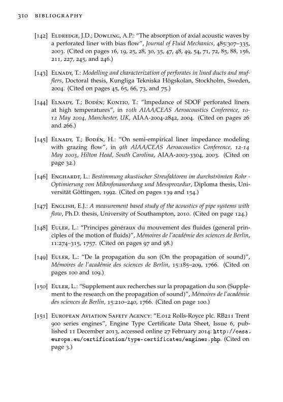
310 bibliography
[142] Eldredge, J.D.; Dowling, A.P.: “The absorption of axial acoustic waves bya perforated liner with bias flow”, Journal of Fluid Mechanics, 485:307–335,2003. (Cited on pages 16, 19, 25, 28, 30, 35, 47, 48, 49, 54, 71, 72, 85, 88, 156,211, 227, 245, and 246.)
[143] Elnady, T.: Modelling and characterization of perforates in lined ducts and muf-flers, Doctoral thesis, Kungliga Tekniska Högskolan, Stockholm, Sweden,2004. (Cited on pages 45, 65, 66, 73, and 75.)
[144] Elnady, T.; Bodén; Kontio, T.: “Impedance of SDOF perforated linersat high temperatures”, in 10th AIAA/CEAS Aeroacoustics Conference, 10-12 May 2004, Manchester, UK, AIAA-2004-2842, 2004. (Cited on pages 26and 266.)
[145] Elnady, T.; Bodén, H.: “On semi-empirical liner impedance modelingwith grazing flow”, in 9th AIAA/CEAS Aeroacoustics Conference, 12-14May 2003, Hilton Head, South Carolina, AIAA-2003-3304, 2003. (Cited onpage 32.)
[146] Enghardt, L.: Bestimmung akustischer Streufaktoren im durchströmten Rohr -Optimierung von Mikrofonanordung und Messprozedur, Diploma thesis, Uni-versität Göttingen, 1992. (Cited on pages 139 and 154.)
[147] English, E.J.: A measurement based study of the acoustics of pipe systems withflow, Ph.D. thesis, University of Southampton, 2010. (Cited on page 124.)
[148] Euler, L.: “Principes généraux du mouvement des fluides (general prin-ciples of the motion of fluids)”, Mémoires de l’académie des sciences de Berlin,11:274–315, 1757. (Cited on pages 97 and 98.)
[149] Euler, L.: “De la propagation du son (On the propagation of sound)”,Mémoires de l’académie des sciences de Berlin, 15:185–209, 1766. (Cited onpages 100 and 109.)
[150] Euler, L.: “Supplement aux recherches sur la propagation du son (Supple-ment to the research on the propagation of sound)”, Mémoires de l’académiedes sciences de Berlin, 15:210–240, 1766. (Cited on page 100.)
[151] European Aviation Safety Agency: “E.012 Rolls-Royce plc. RB211 Trent900 series engines”, Engine Type Certificate Data Sheet, Issue 6, pub-lished 11 December 2013, accessed online 27 February 2014: http://easa.europa.eu/certification/type-certificates/engines.php. (Cited onpage 3.)
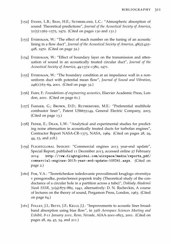
bibliography 311
[152] Evans, L.B.; Bass, H.E.; Sutherland, L.C.: “Atmospheric absorption ofsound: Theoretical predictions”, Journal of the Acoustical Society of America,51(5):1565–1575, 1972. (Cited on pages 130 and 131.)
[153] Eversman, W.: “The effect of mach number on the tuning of an acousticlining in a flow duct”, Journal of the Acoustical Society of America, 48(2):425–428, 1970. (Cited on page 32.)
[154] Eversman, W.: “Effect of boundary layer on the transmission and atten-uation of sound in an acoustically treated circular duct”, Journal of theAcoustical Society of America, 49:1372–1380, 1971.
[155] Eversman, W.: “The boundary condition at an impedance wall in a non-uniform duct with potential mean flow”, Journal of Sound and Vibration,246(1):63–69, 2001. (Cited on page 32.)
[156] Fahy, F.: Foundations of engineering acoustics, Elsevier Academic Press, Lon-don, 2001. (Cited on page 61.)
[157] Farmer, G.; Brown, D.D.; Rutherford, M.E.: “Preferential multiholecombustor liner”, Patent US6655149, General Electric Company, 2003.(Cited on page 13.)
[158] Feder, E.; Dean, L.W.: “Analytical and experimental studies for predict-ing noise attenuation in acoustically treated ducts for turbofan engines”,Contractor Report NASA-CR-1373, NASA, 1969. (Cited on pages 28, 29,44, 53, and 218.)
[159] Flightglobal Insight: “Commercial engines 2013 year-end update”,Special Report, published 11 December 2013, accessed online 27 February2014: http://www.flightglobal.com/airspace/media/reports_pdf/
commercial-engines-2013-year-end-update-108241.aspx. (Cited onpage 2.)
[160] Fok, V.A.: “Teoreticheskoe issledovanie provodimosti kruglogo otverstiyav peregorodke, postavlennoi poperek truby (Theoretical study of the con-ductance of a circular hole in a partition across a tube)”, Doklady AkademiiNauk SSSR, 31(9):875–882, 1941, alternatively: D. N. Rschevkin, A courseof lectures on the theory of sound, Pergamon Press, London, 1963. (Citedon page 64.)
[161] Follet, J.I.; Betts, J.F.; Kelly, J.J.: “Improvements to acoustic liner broad-band absorption using bias flow”, in 39th Aerospace Sciences Meeting andExhibit, 8-11 January 2001, Reno, Nevada, AIAA-2001-0823, 2001. (Cited onpages 28, 29, 45, 54, and 211.)
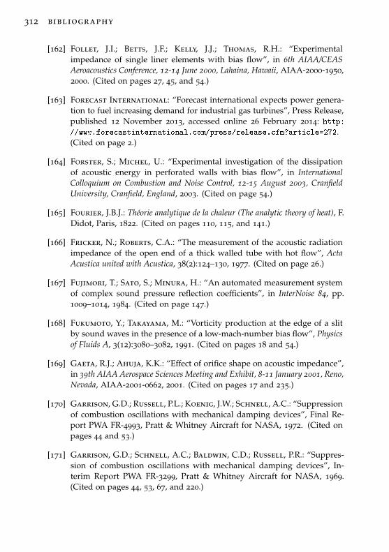
312 bibliography
[162] Follet, J.I.; Betts, J.F.; Kelly, J.J.; Thomas, R.H.: “Experimentalimpedance of single liner elements with bias flow”, in 6th AIAA/CEASAeroacoustics Conference, 12-14 June 2000, Lahaina, Hawaii, AIAA-2000-1950,2000. (Cited on pages 27, 45, and 54.)
[163] Forecast International: “Forecast international expects power genera-tion to fuel increasing demand for industrial gas turbines”, Press Release,published 12 November 2013, accessed online 26 February 2014: http://www.forecastinternational.com/press/release.cfm?article=272.(Cited on page 2.)
[164] Forster, S.; Michel, U.: “Experimental investigation of the dissipationof acoustic energy in perforated walls with bias flow”, in InternationalColloquium on Combustion and Noise Control, 12-15 August 2003, CranfieldUniversity, Cranfield, England, 2003. (Cited on page 54.)
[165] Fourier, J.B.J.: Théorie analytique de la chaleur (The analytic theory of heat), F.Didot, Paris, 1822. (Cited on pages 110, 115, and 141.)
[166] Fricker, N.; Roberts, C.A.: “The measurement of the acoustic radiationimpedance of the open end of a thick walled tube with hot flow”, ActaAcustica united with Acustica, 38(2):124–130, 1977. (Cited on page 26.)
[167] Fujimori, T.; Sato, S.; Minura, H.: “An automated measurement systemof complex sound pressure reflection coefficients”, in InterNoise 84, pp.1009–1014, 1984. (Cited on page 147.)
[168] Fukumoto, Y.; Takayama, M.: “Vorticity production at the edge of a slitby sound waves in the presence of a low-mach-number bias flow”, Physicsof Fluids A, 3(12):3080–3082, 1991. (Cited on pages 18 and 54.)
[169] Gaeta, R.J.; Ahuja, K.K.: “Effect of orifice shape on acoustic impedance”,in 39th AIAA Aerospace Sciences Meeting and Exhibit, 8-11 January 2001, Reno,Nevada, AIAA-2001-0662, 2001. (Cited on pages 17 and 235.)
[170] Garrison, G.D.; Russell, P.L.; Koenig, J.W.; Schnell, A.C.: “Suppressionof combustion oscillations with mechanical damping devices”, Final Re-port PWA FR-4993, Pratt & Whitney Aircraft for NASA, 1972. (Cited onpages 44 and 53.)
[171] Garrison, G.D.; Schnell, A.C.; Baldwin, C.D.; Russell, P.R.: “Suppres-sion of combustion oscillations with mechanical damping devices”, In-terim Report PWA FR-3299, Pratt & Whitney Aircraft for NASA, 1969.(Cited on pages 44, 53, 67, and 220.)
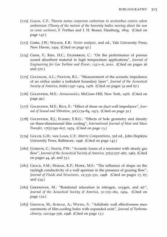
bibliography 313
[172] Gauss, C.F.: Theoria motus corporum coelestium in sectionibus conicis solemambientum (Theory of the motion of the heavenly bodies moving about the sunin conic sections), F. Perthes and I. H. Besser, Hamburg, 1809. (Cited onpage 147.)
[173] Gibbs, J.W.; Wilson, E.B.: Vector analysis, 2nd ed., Yale University Press,New Haven, 1929. (Cited on page 97.)
[174] Giese, F.; Ries, H.C.; Eigenbrod, C.: “On the performance of poroussound absorbent material in high temperature applications”, Journal ofEngineering for Gas Turbine and Power, 132:1–6, 2010. (Cited on pages 26and 270.)
[175] Goldman, A.L.; Panton, R.L.: “Measurement of the acoustic impedanceof an orifice under a turbulent boundary layer”, Journal of the AcousticalSociety of America, 60(6):1397–1404, 1976. (Cited on pages 32 and 67.)
[176] Goldstein, M.E.: Aeroacoustics, McGraw-Hill, New York, 1976. (Cited onpage 99.)
[177] Goldstein, M.E.; Rice, E.: “Effect of shear on duct wall impedance”, Jour-nal of Sound and Vibration, 30(1):79–84, 1973. (Cited on page 32.)
[178] Goldstein, R.J.; Eckert, E.R.G.: “Effects of hole geometry and densityon three-dimensional film cooling”, International Journal of Heat and MassTransfer, 17(5):595–607, 1974. (Cited on page 13.)
[179] Golub, G.H.; van Loan, C.F.: Matrix Computations, 3rd ed., John HopkinsUniversity Press, Baltimore, 1996. (Cited on page 145.)
[180] Gordon, C.; Smith, P.W.: “Acoustic losses of a resonator with steady gasflow”, Journal of the Acoustical Society of America, 37(2):257–267, 1965. (Citedon pages 44, 46, and 53.)
[181] Grace, S.M.; Horan, K.P.; Howe, M.S.: “The influence of shape on therayleigh conductivity of a wall aperture in the presence of grazing flow”,Journal of Fluids and Structures, 12:335–351, 1998. (Cited on pages 17, 67,and 234.)
[182] Greenspan, M.: “Rotational relaxation in nitrogen, oxygen, and air”,Journal of the Acoustical Society of America, 31:155–160, 1959. (Cited onpage 132.)
[183] Gritsch, M.; Schulz, A.; Wittig, S.: “Adiabatic wall effectiveness mea-surements of film-cooling holes with expanded exits”, Journal of Turboma-chinery, 120:549–556, 1998. (Cited on page 13.)
314 bibliography
[184] Gritsch, M.; Schulz, A.; Wittig, S.: “Method for correlating discharge co-efficients of film-cooling holes”, AIAA Journal, 36(6):976–980, 1998. (Citedon page 38.)
[185] Gritsch, M.; Schulz, A.; Wittig, S.: “Effect of crossflows on the dischargecoefficients of film cooling holes with varying angles of inclination and ori-entation”, Journal of Turbomachinery, 123:781–787, 2001. (Cited on page 38.)
[186] Guess, A.W.: “Calculation of perforated plate liner parameters from spec-ified acoustic resistance and reactance”, Journal of Sound and Vibration,40(1):119–137, 1975. (Cited on pages 64, 65, and 67.)
[187] Gullaud, E.; Mendez, S.; Sensiau, C.; Nicoud, F.; Pionsot, T.: “Effect ofmultiperforated plates on the acoustic modes in combustors”, in 2nd Ini-tiative on Advanced Combustion (INCA) Workshop, 23-24 October 2008, Rouen,France, 2008. (Cited on page 55.)
[188] Gullaud, E.; Mendez, S.; Sensiau, C.; Wolf, P.; Nicoud, F.: “Dampingeffect of perforated plates on the acoustics of annular combustors”, in15th AIAA/CEAS Aeroacoustics Conference, 11-13 May 2009, Miami, Florida,AIAA-2009-3260, 2009. (Cited on page 55.)
[189] Gysling, D.L.; Copeland, G.S.; McCormick, D.C.; Proscia, W.M.: “Com-bustion system damping augmentation with helmholtz resonators”, Jour-nal of Engineering for Gas Turbines and Power, 122:269–274, 2000. (Cited onpage 6.)
[190] Harrje, D.T.; Reardon, F.H. (Eds.): Liquid propellant rocket combustion in-stability, NASA-SP-194, NASA, Washington, D.C., 1972. (Cited on page 5.)
[191] Haufe, D.; Fischer, A.; Czarske, J.; Schulz, A.; Bake, F.; Enghardt, L.:“High dynamic range measurements of acoustic particle velocity and flowvelocity for the application at liners”, in 19th AIAA/CEAS AeroacousticsConference, 27-29 May 2013, Berlin, Germany, AIAA-2013-2053, 2013. (Citedon page 51.)
[192] Haufe, D.; Fischer, A.; Czarske, J.; Schulz, A.; Bake, F.; Enghardt, L.:“Multi-scale measurement of acoustic particle velocity and flow velocityfor liner investigations”, Experiments in Fluids, 54:1569, 2013. (Cited onpage 51.)
[193] Heaviside, O.: “Electromagnetic induction and its propagation”, The Elec-trician, 17:212, 1886, reprinted in: Electrical Papers Vol. 2, Section 29, p.61-71, Macmillan & Co., 1894. (Cited on page 59.)
bibliography 315
[194] Heidelberg, L.J.; Rice, E.J.: “Experimental evaluation of a spinning-modeacoustic-treatment design concept for aircraft inlets”, Technical PaperNASA-TP-1613, NASA, 1980. (Cited on page 67.)
[195] von Helmholtz, H.: “Über den Einfluss der Reibung in der Luft auf dieSchallbewegung”, Verhandlungen des Naturhistorisch-Medizinischen Vereinszu Heidelberg, 56(17):257–260, 1863. (Cited on pages 62 and 114.)
[196] Herzfeld, K.F.; Litovitz, T.A.: Absorption and dispersion of ultrasonic waves,Academic Press, New York, 1959. (Cited on page 131.)
[197] Heuwinkel, C.: Experimentelle Untersuchung der akustischen Eigenschaftenperforierter Liner, Diploma thesis, Technische Universität Berlin, 2006.(Cited on pages 54 and 161.)
[198] Heuwinkel, C.; Enghardt, L.; Röhle, I.: “Experimental investigationof the acoustic damping of perforated liners with bias flow”, in 13thAIAA/CEAS Aeroacoustics Conference, 21-23 May 2007, Rome, Italy, AIAA-2007-3525, 2007. (Cited on pages 16, 54, 139, and 211.)
[199] Heuwinkel, C.; Mühlbauer, B.; Busse, S.; Enghardt, L.; Noll, B.;Aigner, M.; Röhle, I.: “Comparison of experimental and numerical re-sults concerning the damping of perforated liners with bias flow”, inASME Turbo Expo 2008, 9-13 June 2008, Berlin, Germany, GT2008-50585,2008. (Cited on pages 28, 30, 55, 202, and 203.)
[200] Heuwinkel, C.; Pardowitz, B.; Bake, F.; Röhle, I.; Enghardt, L.: “Onthe excitation of a zero mass flow liner for acoustic damping”, in 15thAIAA/CEAS Aeroacoustics Conference, 11-13 May 2009, Miami, FL, AIAA-2009-3110, 2009. (Cited on pages 34 and 52.)
[201] Heuwinkel, C.; Piot, E.; Fischer, A.; Röhle, I.; Micheli, F.; Enghardt,L.; Bake, F.: “Characterization of a perforated liner by acoustic and opti-cal measurements”, in 16th AIAA/CEAS Aeroacoustics Conference, 7-9 June,Stockholm, Sweden, AIAA-2010-3765, 2010. (Cited on pages 51, 55, and 281.)
[202] Heuwinkel, C.; Sadig, S.; Gerendás, M.; Enghardt, L.; Bake, F.: “Es-tablishment of a high quality database for the modelling of perforatedliners”, in ASME Turbo Expo 2010, 14-18 June 2010, Glasgow, UK, GT2010-22329, 2010. (Cited on page 55.)
[203] Hofmans, G.C.J.; Boot, R.J.J.; Durrieu, P.P.J.M.; Auregan, Y.;Hirschberg, A.: “Aeroacoustics response of a slit-shaped diaphragm in apipe at low Helmholtz number, 1: Quasi-steady results”, Journal of Soundand Vibration, 244(1):35–56, 2001. (Cited on pages 18 and 54.)
316 bibliography
[204] Hofmans, G.C.J.; Ranucci, M.; Ajello, G.; Auregan, Y.; Hirschberg,A.: “Aeroacoustics response of a slit-shaped diaphragm in a pipe at lowHelmholtz number, 2: Unsteady results”, Journal of Sound and Vibration,244(1):57–77, 2001. (Cited on page 18.)
[205] Holmberg, A.; Åbom, M.; Bodén, H.: “Accurate experimental two-portanalysis of flow generated sound”, Journal of Sound and Vibration, 330:6336–6354, 2011. (Cited on page 124.)
[206] Holste, F.: Ermittlung der aerodynamische Lärmquellen und Berechnung desabgestrahlten Schall mittels der im Nahfeld gemessenen Druckschwankungenam Beispiel eines Triebwerksmodells, Doctoral thesis, Techische UniversitätBerlin, 1995, published in: Fortschritt-Berichte VDI, Series 7, No. 272, VDI,Düsseldorf, 1995. (Cited on page 101.)
[207] Howe, M.S.: “Contributions to the theory of aerodynamic sound, withapplication to excess jet noise and the theory of the flute”, Journal of FluidMechanics, 71:625–673, 1975. (Cited on pages 47 and 100.)
[208] Howe, M.S.: “Attenuation of sound in a low mach number nozzle flow”,Journal of Fluid Mechanics, 91(2):209–229, 1979. (Cited on pages 47 and 53.)
[209] Howe, M.S.: “The influence of grazing flow on the acoustic impedanceof a cylindrical wall cavity”, Journal of Sound and Vibration, 67(4):533–544,1979. (Cited on pages 32 and 67.)
[210] Howe, M.S.: “On the theory of unsteady high reynolds number flowthrough a circular aperture”, Proceedings of the Royal Society of London,366:205–223, 1979. (Cited on pages 35, 47, 48, 53, 68, 69, 70, 73, 74, and 271.)
[211] Howe, M.S.: “On the absorption of sound by turbulence and other hydro-dynamic flows”, Journal of Applied Mathematics, 32:187–209, 1984. (Citedon page 126.)
[212] Howe, M.S.: “The damping of sound by wall turbulent shear layers”, Jour-nal of the Acoustical Society of America, 98(3):1723–1730, 1995. (Cited onpages 126, 127, and 129.)
[213] Howe, M.S.: “Influence of cross-sectional shape on the conductivity of awall aperture in mean flow”, Journal of Sound and Vibration, 207:601–616,1997. (Cited on pages 17 and 18.)
[214] Howe, M.S.: Acoustics of fluid-structure interactions, Cambridge UniversityPress, Cambridge, UK, 1998. (Cited on pages 35, 47, 58, 68, 69, 85, 100,118, 126, 127, and 129.)
bibliography 317
[215] Howe, M.S.; Scott, M.I.; Sipcic, S.R.: “The influence of tangential meanflow on the rayleigh conductivity of an aperture”, Proceedings of the RoyalSociety of London, Series A, 452(1953):2303–2317, 1996. (Cited on page 32.)
[216] Hrubes, J.D.: Flow generated noise of acoustical duct liners, Master’s thesis,Massachusetts Institute of Technology, 1977. (Cited on page 219.)
[217] Hu, Y.: Développement de panneaux hybrides passifs/actifs pour l’acoustique (De-velopment of hybrid passive/active acoustic panels), Doctoral thesis, Ecole Cen-trale de Lyon, 2010. (Cited on page 294.)
[218] Hudde, H.; Letens, U.: “Untersuchungen zum akustischenMeßleitungsverfahren mit festen Meßorten”, Acustica, 56(4):258–269,1984. (Cited on page 146.)
[219] Hughes, I.J.; Dowling, A.P.: “The absorption of sound by perforated lin-ings”, Journal of Fluid Mechanics, 218:299–335, 1990. (Cited on pages 25, 35,47, 51, 54, 71, 88, 211, 227, 252, and 271.)
[220] ICAO: “Manual of the ICAO standard atmosphere”, Doc 7488/3, Interna-tional Civil Aviation Organization, 1993. (Cited on pages 122 and 284.)
[221] Idelchick, I.E.: Handbook of hydraulic resistance, 3rd ed., Jaico PublishingHouse, Mumbai, India, 2011. (Cited on page 38.)
[222] Igarashi, J.; Toyama, M.: “Fundamentals of acoustic silencers, Part 1: The-ory and experiments of acoustic low-pass filters”, Report 339, Universityof Tokyo, 1958. (Cited on page 80.)
[223] Imelmann, C.: Einfluß der Strömung auf den Schalldurchgang durch Rohrmün-dungen (Influence of flow on the sound transmission through orifices), Diplomathesis, Technische Universiät Berlin, 1978. (Cited on page 53.)
[224] Imelmann, C.: “Schallabsorption in durchströmten Rohrmündungen”, inFortschritte der Akustik, DAGA ’80, München, pp. 493–496, VDE-Verlag,Berlin, 1980. (Cited on page 53.)
[225] Ingard, U.: “On the theory and design of acoustic resonators”, Journal ofthe Acoustical Society of America, 25(6):1037–1062, 1953. (Cited on pages 17,28, 45, 59, 63, 64, 65, 74, 77, 202, and 233.)
[226] Ingard, U.: “Attenuation and regeneration of sound in ducts and jet dif-fusers”, Journal of the Acoustical Society of America, 31(9):1202–1212, 1959.(Cited on pages 44, 53, and 217.)
318 bibliography
[227] Ingard, U.; Ising, H.: “Acoustic nonlinearity of an orifice”, Journal of theAcoustical Society of America, 42:6–17, 1967. (Cited on pages 28, 44, 45, 53,65, 67, and 202.)
[228] Ingard, U.; Labate, S.: “Acoustic circulation effects and the nonlinearimpedance of orifices”, Journal of the Acoustical Society of America, 22(2):211–218, 1950. (Cited on pages 28, 45, 65, and 202.)
[229] Ingard, U.; Singhal, V.K.: “Sound attenuation in turbulent pipe flow”,Journal of the Acoustical Society of America, 55(3):535–538, 1974. (Cited onpage 126.)
[230] International Air Transport Association: “Airlines expect 31 % risein passenger demand by 2017”, Press Release 67, published 10 De-cember 2013, accessed online 25 February 2014: http://www.iata.org/pressroom/pr/pages/2013-12-10-01.aspx. (Cited on page 2.)
[231] International Energy Agency: “Key world energy statistics 2013”, Re-port, published 2013, accessed online27 February 2014: http://www.iea.org/publications/freepublications/publication/KeyWorld2013.pdf.(Cited on page 1.)
[232] ISO 10534-2:1998: “Acoustics - Determination of sound absorptioncoefficient and impedance in impedance tubes - Part 2: Transfer-function method”, Standard, International Organization for Standardiza-tion, Geneva, Switzerland, 1998. (Cited on page 146.)
[233] ISO 5136:2003: “Acoustics - Determination of sound power radiated into aduct by fans and other air-moving devices - In-duct method”, Standard, In-ternational Organization for Standardization, Geneva, Switzerland, 2003.(Cited on page 165.)
[234] ISO 5167-2:2003: “Measurement of fluid flow by means of pressure differ-ential devices inserted in circular cross-section conduits running full, Part2: Orifice plates”, Standard, International Organization for Standardiza-tion, Geneva, Switzerland, 2003. (Cited on pages 19 and 36.)
[235] ISO 80000-8:2007: “Quantities and units - Part 8: Acoustics”, Standard, In-ternational Organization for Standardization, Geneva, Switzerland, 2007.(Cited on page 113.)
[236] ISO 9613-1:1993: “Acoustics - Attenuation of sound during propagationoutdoors - Part 1”, Report, International Organization for Standardization,Geneva, Switzerland, 1993. (Cited on pages 130, 133, and 134.)
bibliography 319
[237] Jang, S.H.; Ih, J.: “On the multiple microphone method for measuringin-duct acoustic properties in the presence of mean flow”, Journal of theAcoustical Society of America, 103(3):1520–1526, 1998. (Cited on page 147.)
[238] Janus, M.C.; Richards, G.M.; Yip, M.J.: “Effects of ambient conditionsand fuel composition on combustion stability”, in ASME Turbo Expo 1997,2-5 June 1997, Orlando, Florida, USA, GT1997-266, 1997. (Cited on page 5.)
[239] Jayaraman, K.; Yam, K.: “Decoupling approach to modeling perforatedtube muffler components”, Journal of the Acoustical Society of America,69(2):390–396, 1981. (Cited on page 82.)
[240] Jayatunga, C.; Qin, Q.; Sanderson, V.; Rubini, P.; You, D.; Krebs, W.:“Absorption of normal-incedence acoustic waves by double perforated lin-ers of industrial gas turbine combustors”, in Proceedings of ASME TurboExpo 2012, 11-15 June 2012, Copenhagen, Denmark, GT2012-68842, 2012.(Cited on pages 55 and 249.)
[241] Jing, X.; Sun, X.: “Experimental investigation of perforated liners withbias flow”, Journal of the Acoustical Society of America, 106(5):2436–2441,1999. (Cited on pages 25, 34, 47, 48, 54, 71, 72, 88, 211, 227, and 231.)
[242] Jing, X.; Sun, X.: “Effect of plate thickness on impedance of perforatedplates with bias flow”, AIAA Journal, 38(9):1573–1578, 2000. (Cited onpages 48, 54, 68, 72, 77, 93, 212, 251, 271, and 280.)
[243] Jing, X.; Sun, X.: “Sound-excited flow and acoustic nonlinearity at an ori-fice”, Physics of Fluids, 14(1):268–276, 2002. (Cited on pages 28, 29, 45,and 202.)
[244] Jing, X.; Sun, X.; Wu, J.; Meng, K.: “Effect of grazing flow on the acousticimpedance of an orifice”, AIAA Journal, 39(8):1478–1484, 2001. (Cited onpages 32 and 67.)
[245] Johnston, J.P.; Schmidt, W.E.: “Measurement of acoustic reflection froman obstruction in a pipe with flow”, Journal of the Acoustic Society of America,63:1455–1460, 1978. (Cited on page 146.)
[246] Jones, M.G.: “Evaluation of a multi-point method for determining acous-tic impedance”, Mechanical Systems and Signal Processing, 3(1):15–35, 1989.(Cited on page 147.)
[247] Jones, M.G.; Howerton, B.M.; Busse-Gerstengarbe, S.: “Comparativestudy of impedance eduction methods, Part 2: NASA tests and methodol-ogy”, in 19th AIAA/CEAS Aeroacoustics Conference, 27-29 May 2013, Berlin,Germany, AIAA-2013-2125, 2013. (Cited on pages 27 and 28.)
320 bibliography
[248] Jones, M.G.; Watson, W.R.: “On the use of experimental methods to im-prove confidence in educed impedance”, in 17th AIAA/CEAS AeroacousticsConference, 5-8 June 2011, Portland, Oregon, AIAA-2011-2865, 2011. (Citedon page 30.)
[249] Jordan, C.: “Mémoire sur les formes bilinéaires”, Journal de MathématiquesPures et Appliquées, Deuxiéme Série, 19:35–54, 1874. (Cited on page 145.)
[250] Jordan, C.: “Sur la réduction des formes bilinéaires”, Comptes Rendus del’Académie des Sciences, Paris, 78:614–617, 1874. (Cited on page 145.)
[251] Jörg, C.; Gikadi, J.; Sattelmayer, T.: “Numerical investigation of theplane-wave reflection coefficient of an exhaust pipe at elevated tempera-tures using linearized Navier-Stokes equations”, in ASME Turbo Expo 2013,GT2013, 3-7 June 2013, San Antonio,Texas, USA, GT2013-94843, 2013. (Citedon page 26.)
[252] Jörg, C.; Wagner, M.; Sattelmayer, T.: “Experimental investigation ofthe acoustic reflection coefficient of a modeled gas turbine impingementcooling section”, in ASME Turbo Expo 2012, 11-15 June 2012, Copenhage,Denmark, GT2012-68916, 2012. (Cited on page 55.)
[253] Jung, I.S.; Lee, J.S.: “Effects of orientation angles on film cooling over aflat plate: Boundary layer temperature distributions and adiabatic filmcooling effectiveness”, Journal of Turbomachinery, 122:153–160, 2000. (Citedon page 13.)
[254] Kaddah, K.S.: Discharge coefficient and jet deflection studies for combustorliner air entry holes, Diploma thesis, Cranfield University, 1964. (Cited onpage 38.)
[255] Kameier, F.: Experimentelle Untersuchung zur Entstehung und Minderung desBlattspitzen-Wirbellärms axialer Strömungsmachinen, Doctoral thesis, Tech-nische Universität Berlin, 1993. (Cited on page 108.)
[256] von Kármán, T.: “Mechanische ähnlichkeit und Turbulenz”, Nachrichtenvon der Gesellschaft der Wissenschaften zu Göttingen (Mathematisch-Physikalische Klasse), pp. 58–76, 1930. (Cited on page 127.)
[257] Keefe, D.H.: “Acoustical wave propagation in cylindrical ducts: Trans-mission line parameter approximations for isothermal and nonisothermalboundary conditions”, Journal of the Acoustical Society of America, 75(1):58–62, 1984. (Cited on pages 113 and 121.)
bibliography 321
[258] Keller, J.J.; Zauner, E.: “On the use of Helmholtz resonators as soundattenuators”, Zeitschrift für angewandte Mathematik und Physik, 46:297–327,1995. (Cited on pages 19, 54, 78, 238, and 239.)
[259] Kim, Y.H.; Yoon, D.B.: “An experimental study on the acoustic character-istics of perforated pipe in terms of wavenumber and porosity”, Journal ofSound and Vibration, 183(1):115–127, 1995. (Cited on page 23.)
[260] Kinsler, L.; Frey, A.; Coppens, A.; Sanders, J.: Fundamentals of acoustics,4th ed., John Wiley and Sons, New York, 2000. (Cited on pages 59, 61, 63,79, 110, and 212.)
[261] Kirchhoff, G.: “Über den Einfluss der Wärmeleitung in einem Gase aufdie Schallbewegung”, Annalen der Physik und Chemie, 210(6):177–193, 1868.(Cited on pages 62, 114, 115, 118, 120, 121, and 131.)
[262] Kirchhoff, G.: “Zur Theorie freier Flüssigkeitsstrahlen”, Journal für Math-ematik, 70:289–298, 1869. (Cited on page 37.)
[263] Knutsson, M.; Åbom, M.: “The effect of turbulence damping on acousticwave propagation in tubes”, Journal of Sound and Vibration, 329:4719–4739,2010. (Cited on page 126.)
[264] Ko, S.H.: “Sound attenuation in acoustically lined circular ducts in thepresence of uniform flow and shear flow”, Journal of Sound and Vibration,22(2):193–210, 1972. (Cited on pages 32 and 217.)
[265] Kompenhans, J.; Ronneberger, D.: “The acoustic impedance of orifices inthe wall of a flow duct with a laminar or turbulent flow boundary layer”,in 6th AIAA Aeroacoustics Conference, 4-6 June 1980. Hartford, Connecticut,AIAA-80-0990, 1980.
[266] Kooi, J.W.; Sarin, S.L.: “An experimental study of the impedance ofhelmholtz resonator arrays under a turbulent boundary layer”, in 7thAIAA Aeroacoustics Conference, 5-7 October 1981, Palo Alto, California, AIAA-1981-1998, 1981. (Cited on pages 32 and 67.)
[267] Kooijman, G.: Acoustical response of shear layers, Doctoral thesis, Technis-che Universiteit Eindhoven, 2007. (Cited on page 18.)
[268] Kooijman, G.; Auregan, Y.; Hirschberg, A.: “Orifice impedance undergrazing flow: Modal expansion approach”, in 11th AIAA/CEAS Aeroacous-tics Conference, 23-25 May 2005, Monterey, California, AIAA-2005-2857, 2005.(Cited on page 32.)
322 bibliography
[269] Kooijman, G.; Hirschberg, A.; Golliard, J.: “Acoustical response of ori-fices under grazing flow: Effect of boundary layer profile and edge geom-etry”, Journal of Sound and Vibration, 315:849–874, 2008. (Cited on page 19.)
[270] Kovasznay, L.S.G.: “Turbulence in supersonic flow”, Journal of the Aeronau-tical Sciences, 20(10):657–674, 682, 1953. (Cited on page 115.)
[271] Kraft, R.E.; Yu, J.; Kwan, H.W.: “Acoustic treatment design scaling meth-ods, Vol. 2: Advanced treatment impedance models for high frequencyranges”, Contractor Report NASA-CR-1999-209120 Vol. 2, NASA, 1999.(Cited on pages 61, 62, 65, 66, and 75.)
[272] Krebs, W.; Bethke, S.; Lepers, J.; Flohr, P.; Prade, B.; Johnson, C.; Sat-tinger, S.: “Thermoacoustic design tools and passive control: SiemensPower Generation approaches”, in [305], Chap. 5, pp. 89–112, 2005. (Citedon page 15.)
[273] Kundt, A.: “Untersuchungen über die Schallgeschwindigkeit der Luft inRöhren”, Annalen der Physik, 135(11):337–372, 1868. (Cited on pages 114and 190.)
[274] Kurze, U.J.; Allen, C.H.: “Influence of flow and high sound level on theattenuation in a lined duct”, Journal of the Acoustical Society of America,49(5):1643–1654, 1971. (Cited on pages 32 and 217.)
[275] Kutta, W.M.: Über die Strömung einer Flüssigkeit um in sie versenkte zylin-drische Flächen und den Druck, den diese dabei erfahren, Habilitation thesis,Technische Hochschule München, 1902. (Cited on page 46.)
[276] Kwan, H.W.; Yu, J.; Beer, B.; Armitage, D.: “Bias flow adaptive acousticliner”, in AIAA Meeting Paper Archive 172, AIAA-1999-1939, 1999. (Citedon pages 34, 45, and 54.)
[277] Lahiri, C.; Knobloch, K.; Bake, F.; Enghardt, L.: “Acoustic measure-ments of perforated liners in hot and pressurized flow”, in ASME TuboExpo 2013, 3-7 June 2013, San Antonio, Texas, USA, GT2013-94674, 2013.(Cited on pages 52 and 190.)
[278] Lahiri, C.; Knobloch, K.; Bake, F.; Enghardt, L.: “Attenuation of soundin wide ducts with flow at elevated pressure and temperature”, Journal ofSound and Vibration, 333(15):3440–3458, 2014. (Cited on pages 190 and 191.)
[279] Lahiri, C.; Knobloch, K.; Sadig, S.; Bake, F.: “Influence of cavity designon the performance of hot-stream bias flow liners”, in 18th AIAA/CEASAeroacoustics Conference, 4-6 June 2012, Colorado Springs, Colorado, AIAA-2012-2200, 2012. (Cited on pages 16, 52, and 55.)
bibliography 323
[280] Lahiri, C.; Pardowitz, B.; Bake, F.; Enghardt, L.: “The application ofan aeroacoustic actuator in a zero mass flow liner for acoustic damping”,in 17th AIAA/CEAS Aeroacoustics Conference, 05 - 08 June 2011, Portland,Oregon, AIAA-2011-2725, 2011. (Cited on pages 34 and 52.)
[281] Lahiri, C.; Pardowitz, B.; Bake, F.; Röhle, I.; Enghardt, L.: “Excitationof a zero mass flow liner for acoustic damping”, AIAA Journal, 49(3):513–519, 2011. (Cited on pages 32, 34, 52, and 262.)
[282] Lahiri, C.; Sadig, S.; Gerendás, M.; Enghardt, L.; Bake, F.: “Establish-ment of a high quality database for the acoustic modeling of perforatedliners”, Journal of Engineering for Gas Turbines and Power, 133:1–9, 2011.(Cited on pages 17, 19, 23, 25, 27, 35, 47, 48, 52, 55, 71, and 72.)
[283] Landau, L.D.; Lifshitz, E.M.: Fluid Mechanics, 3rd ed., Pergamon Press,Oxford, 1966. (Cited on pages 39, 114, and 115.)
[284] Laudien, E.; Pongratz, R.; Pierro, R.; Preclik, D.: “Experimental proce-dures aiding the design of acoustic cavities”, in [497], Chap. 14, pp. 377–399, 1995. (Cited on pages 6, 19, 109, and 238.)
[285] Laurens, S.; Piot, E.; Bendali, A.; Fares, M.B.; Tordaux, S.: “Effectiveconditions for the reflection of an acoustic wave by low-porosity per-forated plates”, Journal of Fluid Mechanics, 743:448–480, 2014. (Cited onpages 47 and 246.)
[286] Laurens, S.; Tordeux, S.; Bendali, A.; Fares, M.; Kotiuga, P.R.: “Lowerand upper bounds for the Rayleigh conductivity of a perforated plate”,ESAIM: Mathematical Modelling and Numerical Analysis, 47(6):1691–1712,2013. (Cited on pages 19 and 59.)
[287] Lee, D.H.; Kwon, Y.P.: “Estimation of the absorption performance of mul-tiple layer perforated panel systems by transfer matrix method”, Journalof Sound and Vibration, 278:847–860, 2004. (Cited on page 202.)
[288] Lee, I.: Acoustic characteristics of perforated dissipative and hybrid silencers,Ph.d. thesis, Ohio State University, 2005. (Cited on pages 22, 65, 262,and 263.)
[289] Lee, I.; Selamet, A.; Huff, N.T.: “Impact of perforation impedance onthe transmission loss of reactive and dissipative silencers”, Journal of theAcoustical Society of America, 120(6):3706–3713, 2006. (Cited on pages 22,262, and 263.)
324 bibliography
[290] Lee, S.H.; Ih, J.G.: “Emperical model of the acoustic impedance of a circu-lar orifice in grazing mean flow”, Journal of the Acoustical Society of America,114(1):98–113, 2003. (Cited on pages 32, 67, and 75.)
[291] Lee, S.H.; Ih, J.G.; Peat, K.S.: “A model of acoustic impedance of perfo-rated plates with bias flow considering the interaction effect”, Journal ofSound and Vibration, 303:741–752, 2007. (Cited on pages 55, 68, 93, 212,and 280.)
[292] Lefebvre, A.H.; Ballal, D.R.: Gas Turbine Combustion - Alternative Fuelsand Emissions, 3rd ed., CRC Press, Boca Raton, FL, 2010. (Cited on pages 3,4, 12, 13, and 15.)
[293] Legendre, A.M.: Nouvelles methodes pour la determination des orbites descometes (New Methods for the Determination of Comet Orbits), F. Didot, Paris,1805. (Cited on page 147.)
[294] Lei, L.; Zhihui, G.; Chengyu, Z.; Xiaofeng, S.: “A passive method tocontrol combustion instabilities with perforated liner”, Chinese Journal ofAeronautics, 23:623–630, 2010. (Cited on pages 16, 26, and 55.)
[295] Lemmon, E.W.; Jacobsen, R.T.: “Viscosity and thermal conductivity equa-tions for nitrogen, oxygen, argon, and air”, International Journal of Thermo-physics, 25(1):21–69, 2004. (Cited on pages 284 and 285.)
[296] Lemmon, E.W.; Jacobsen, R.T.; Penoncello, S.G.; Friend, D.G.: “Ther-modynamic properties of air and mixtures of nitrogen, argon, and oxygenfrom 60 to 2000 K at pressures to 2000 MPa”, Journal of Physical and Chem-ical Reference Data, 29(3):331–385, 2000. (Cited on pages 284 and 285.)
[297] Leppington, F.G.: “The effective compliance of perforated screens”, Math-ematika, 24:199–215, 1977. (Cited on pages 47 and 227.)
[298] Leppington, F.G.; Levine, H.: “Reflexion and transmission at a planescreen with periodically arranged circular or elliptical apertures”, Journalof Fluid Mechanics, 61(1):109–127, 1973. (Cited on page 227.)
[299] Leung, R.C.K.; So, R.M.C.; Wang, M.H.; Li, X.M.: “In-duct orifice and itseffect on sound absorption”, Journal of Sound and Vibration, 299:990–1004,2007. (Cited on page 55.)
[300] Lewis, G.D.; Garrison, G.D.: “The role of acoustic absorbers in pre-venting combustion instability”, in AIAA/SAE 7th Propulsion Joint Special-ist Conference,14-18 June 1971, Salt Lake City, Utah, AIAA-1971-0699, 1971.(Cited on pages 44 and 220.)
bibliography 325
[301] Lewis Laboratory Staff: “A summary of preliminary investigations intothe characteristics of combustion screech in ducted burners”, TechnicalReport NACA-TR-1384, National Advisory Committee for Aeronautics,1954. (Cited on page 15.)
[302] Lichtarowicz, A.; Duggins, R.K.; Markland, E.: “Discharge coefficientsfor incompressible non-cavitating flow through long orifices”, Journal ofMechanical Engineering Science, 7(2):210–219, 1965. (Cited on page 36.)
[303] Lienhard, J.H.; Lienhard, J.H.: “Velocity coefficients for free jets fromsharp-edged orifices”, Journal of Fluids Engineering, 106:13–17, 1984. (Citedon page 37.)
[304] Lieuwen, T.C.: Unsteady Combustor Physics, Cambridge University Press,New York, NY, 2012. (Cited on page 15.)
[305] Lieuwen, T.C.; Yang, V. (Eds.): Combustion instabilities in gas turbine engines,AIAA, Reston, VA, 2005. (Cited on pages 5, 7, 15, 27, 306, 309, 322, 328,and 343.)
[306] Lieuwen, T.C.; Yang, V. (Eds.): Gas turbine emissions, Cambridge Univer-sity Press, Cambridge, UK, 2013. (Cited on page 3.)
[307] Lung, T.Y.; Doige, A.G.: “A time-averaging transient testing method foracoustic properties of piping systems and mufflers with flow”, Journal ofthe Acoustical Society of America, 73:867–876, 1983. (Cited on page 154.)
[308] Luong, T.; Howe, M.S.; McGowan, R.S.: “On the Rayleigh conductivityof a bias-flow aperture”, Journal of Fluids and Structures, 21:769–778, 2005.(Cited on pages 48, 54, 73, 74, and 203.)
[309] Lutz, O.: “Resonanzschwingungen in den Rohrleitungen von Kolben-maschinen (Resonant oscillations in the ducts of reciprocating engines)”,Berichte aus dem Laboratorium für Verbrennungskraftmaschinen der TechnischenHochschule Stuttgart, 3:17–110, 1934. (Cited on pages 43 and 53.)
[310] Macquisten, M.A.; Holt, A.; Whiteman, M.; Moran, A.J.; Rupp, J.: “Pas-sive damper lp tests for controlling combustion instability”, in ASMETurbo Expo 2006, 8-11 May 2006, Barcelona, Spain, GT2006-90874, 2006.(Cited on pages 16, 25, 26, 27, 55, 72, 211, and 269.)
[311] Maier, W.; Lutz, O.: “Resonanzerscheinungen in den Rohrleitungen vonVerbrennungskraftmaschinen (Resonance phenomena in the ducts of com-bustion engines)”, Berichte aus dem Laboratorium für Verbrennungskraft-maschinen der Technischen Hochschule Stuttgart, 3:1–16, 1934. (Cited onpages 43 and 53.)
326 bibliography
[312] Malmary, C.; Carbonne, S.; Auregan, Y.; Pagneux, V.: “Acousticimpedance measurement with grazing flow”, in 7th AIAA/CEAS Aeroacous-tics Conference, 28-30 May 2001, Maastricht, Netherlands, AIAA-2001-2193,2001. (Cited on page 32.)
[313] Marino, P.A.; Bohn, N.; Russell, P.L.; Schnell, A.C.; Parson, G.L.:“A study of the suppression of combustion oscillations with mechani-cal damping devices”, Contractor Report NASA-CR-90094, NASA, 1967.(Cited on pages 220 and 221.)
[314] Markham, J.J.; Beyer, R.T.; Lindsay, R.B.: “Absorption of sound in fluids”,Reviews of Modern Physics, 23(4):353–411, 1951. (Cited on page 131.)
[315] Mason, V.: “Some experiments on the propagation of sound along acylindrical duct containing flowing air”, Journal of Sound and Vibration,10(2):208–226, 1969. (Cited on page 103.)
[316] Mason, W.P.: “The propagation characteristics of sound tubes and acous-tic filters”, Physical Review, 31:283–295, 1928. (Cited on page 190.)
[317] Mazdeh, A.; Kashani, R.: “Distributed parameter acoustic modeling ofa perforation with bias flow”, in ASME Turbo Expo 2011, 6-10 June 2001,Vancouver, Canada, GT2011-46649, 2011. (Cited on pages 47, 51, 55, and 71.)
[318] Mazdeh, A.; Kashani, R.: “The impact of perforation geometry on acous-tic damping attributes of a perforated liner with bias flow”, in ASMETurbo Expo 2012, 11-15 June 2012, Copenhagen, Denmark, GT2012-69727,2012. (Cited on pages 47, 51, 55, and 71.)
[319] McAuliffe, C.E.: The influence of high speed flow on the bahavior of acousticalelements, M.Sc. thesis, Massachusetts Institute of Technology, 1950. (Citedon pages 43, 53, and 212.)
[320] McVeigh, J.C.: “Hysteresis in the flow through an orifice”, Nature, 212:918,1966. (Cited on page 36.)
[321] Mechel, F.: “Schalldämpfung und schallverstärkung in luftströmungendurch absorbierend ausgekleidete Kanäle”, Acustica, 10(3):133–148, 1960.(Cited on pages 217 and 219.)
[322] Mechel, F.: “Research on sound propagation in sound-absorbent ductswith superimposed air streams, Vol. 1”, Report AMRL-TDR-62-140(1),Aerospace Medical Research Laboratories, Wright-Patterson Air ForceBase, 1962. (Cited on pages 32 and 217.)
bibliography 327
[323] Mechel, F.: Formulas of acoustics, 2nd ed., Springer, Berlin, 2008. (Cited onpages 80, 81, 82, and 85.)
[324] Mechel, F.; Mertens, P.: “Schallausbreitung in absorbierend ausgeklei-deten Strömungskanälen bei hohen Windgeschwindigkeiten”, Acustica,13(3):154–165, 1963. (Cited on page 217.)
[325] Mechel, F.; Mertens, P.; Schilz, W.: “Interaction between air flow andairborne sound in a duct”, Report AMRL-TR-65-53, Aerospace MedicalResearch Laboratories, Wright-Patterson Air Force Base, 1965. (Cited onpages 44 and 53.)
[326] Mechel, F.; Schilz, W.; Dietz, J.: “Akustische Impedanz einer luftdurch-strömten Öffnung”, Acustica, 15:199–206, 1965. (Cited on pages 44, 53,and 67.)
[327] Melling, T.H.: “The acoustic impedance of perforates at medium andhigh sound pressure levels”, Journal of Sound and Vibration, 29(1):1–65, 1973.(Cited on pages 28, 45, 61, 62, 63, 64, 65, 75, 77, 202, and 227.)
[328] Mendez, S.; Eldredge, J.D.: “Acoustic modeling of perforated plates withbias flow for large-eddy simulations”, Journal of Computational Physics,228(13):4757–4772, 2009. (Cited on pages 55 and 246.)
[329] Meyer, E.; Mechel, F.; Kurtze, G.: “Experiments on the influence of flowon sound attenuation in absorbing ducts”, Journal of the Acoustical Societyof America, 30:165, 1958. (Cited on pages 32 and 217.)
[330] Michalke, A.: “On the propagation of sound generated in a pipe of circu-lar cross-section with uniform mean flow”, Journal of Sound and Vibration,134(2):203–234, 1989. (Cited on page 103.)
[331] Mitsubushi Heavy Industries: “MHI achieves 1,600 °c turbine inlet tem-perature in test operation of world’s highest thermal efficiency j-series gasturbine”, Press Release No. 1435, published 26 May 2011, accessed online27 February 2014: http://www.mhi.co.jp/en/news/story/1105261435.
html. (Cited on pages 2 and 14.)
[332] Moers, E.M.T.; Tonon, D.; Hirschberg, A.: “Sound absorption by perfo-rated walls with bias/grazing flow: Experimental study of the influenceof perforation angle”, in Acoustics 2012, 23-27 April 2012, Nantes, France,2012. (Cited on pages 18, 19, 34, 50, and 55.)
[333] Mongia, H.C.; Held, T.J.; Hsiao, G.C.; Pandalai, R.P.: “Incorporation ofcombustion instability issues into design process: GE aeroderivative and
328 bibliography
aero engine experience”, in [305], Chap. 3, pp. 43–63, 2005. (Cited onpages 6 and 15.)
[334] Moore, E.H.: “On the reciprocal of the general algebraic matrix”, Bul-letin of the American Mathematical Society, 26(9):394–395, 1920. (Cited onpage 145.)
[335] Morfey, C.L.: “Rotating pressure patterns in ducts: Their generation andtransmission”, Journal of Sound and Vibration, 1:60–87, 1964. (Cited onpage 101.)
[336] Morfey, C.L.: “Acoustic properties of openings at low frequencies”, Jour-nal of Sound and Vibration, 9(3):357–366, 1969. (Cited on pages 17, 58, 234,and 235.)
[337] Morfey, C.L.: “Sound transmission and generation in ducts with flow”,Journal of Sound and Vibration, 14(1):37–55, 1971. (Cited on page 103.)
[338] Morfey, C.L.: Dictonary of acoustics, Academic Press, 2001. (Cited onpages 37, 46, 61, 98, 100, 102, and 155.)
[339] Morse, P.M.: Vibration and sound, 2nd ed., McGraw-Hill, New York, 1948.(Cited on page 59.)
[340] Morse, P.M.; Ingard, K.U.: Theoretical acoustics, McGraw-Hill, New York,1968. (Cited on pages 66, 100, 101, 111, and 118.)
[341] Mungur, P.; Whitesides, J.L.: “Influence of grazing flow on duct wall nor-mal impedance”, in 2nd AIAA Aeroacoustics Conference, 24-26 March 1975,Hampton, Virginia, AIAA-1975-0494, 1975. (Cited on page 32.)
[342] Munjal, M.L.: “Velocity ratio-cum-transfer matrix method for the evalua-tion of a muffler with mean flow”, Journal of Sound and Vibration, 39(1):105–119, 1975. (Cited on page 81.)
[343] Munjal, M.L.: Acoustics of ducts and mufflers, John Wiley and Sons, NewYork, 1987. (Cited on pages 80, 81, 82, 100, 103, 109, 110, and 111.)
[344] Munjal, M.L.; Doige, A.G.: “Theory of a two source-location methodfor direct experimental evaluation of the four-pole parameters of anaeroacoustic element”, Journal of Sound and Vibration, 141(2):323–333, 1990.(Cited on page 154.)
[345] Munjal, M.L.; Rao, K.N.; Sahasrabudhe, A.D.: “Aeroacoustic analysis ofperforated muffler components”, Journal of Sound and Vibration, 114(2):173–188, 1987. (Cited on page 82.)
bibliography 329
[346] Munt, R.M.: “The interaction of sound with a subsonic jet issuing from asemi-infinite cylindrical pipe”, Journal of Fluid Mechanics, 83:609–640, 1977.(Cited on pages 26 and 53.)
[347] Munt, R.M.: “Acoustic transmission properties of a jet pipe with subsonicjet flow”, Journal of Sound and Vibration, 142(3):413–436, 1990. (Cited onpage 53.)
[348] Navier, C.L.M.H.: “Memoire sur les lois du mouvement des fluides”,Mémoires de l’Académie des sciences de l’Institut de France, 6:389–440, 1822.(Cited on page 114.)
[349] Nayfeh, A.H.; Kaiser, J.E.; Telionis, D.P.: “Acoustics of aircraft engine-duct systems”, AIAA Journal, 13(2):130–153, 1975. (Cited on page 217.)
[350] Nayfeh, A.H.; Sun, J.: “Effect of transverse velocity and temperature gra-dients on sound attenuation in two-dimensional ducts”, Journal of Soundand Vibration, 34(4):505–517, 1974. (Cited on page 268.)
[351] Nealy, D.A.; Reider, S.B.; Mongia, H.C.: “Alternate cooling configura-tions for gas turbine combustion systems”, in Heat transfer and cooling ingas turbines, AGARD-CP-390, Chap. 25, Advisory Group for AerospaceResearch and Development, 1985. (Cited on page 13.)
[352] Neise, W.; Michel, U.: “Aerodynamic noise of turbomachines”, ReportDLR-IB-22314-94/B5, DLR, 1994. (Cited on page 101.)
[353] Newton, I.: Philosophiae Naturalis Principia Mathematica, Cantabrigiæ,Cambridge, UK, 1713. (Cited on page 36.)
[354] Nilsson, B.; Brander, O.: “The propagation of sound in cylindrical ductswith mean flow and bulk reacting lining: III. Step discontiuities”, Journalof the Institute of Mathematics and its Applications, 27:105–131, 1981. (Citedon page 53.)
[355] Nordin, P.; Sarin, S.L.; Rademaker, E.R.: “Development of new linertechnology for application in hot stream areas of aero-engines”, in 10thAIAA/CEAS Aeroacoustics Conference, 10-12 May 2004, Manchester, UK,AIAA-2004-3033, 2004. (Cited on page 26.)
[356] Norris, A.N.; Sheng, C.: “Acoustic radiation from a circular pipe with aninfinite flange”, Journal of Sound and Vibration, 135:85–93, 1989. (Cited onpage 77.)
330 bibliography
[357] Oberg, C.L.; Wong, T.L.; Ford, W.M.: “Evaluation of acoustic cavities forcombustion stabilization”, Contractor Report NASA-CR-115087, NASA,1971. (Cited on pages 26 and 53.)
[358] Ohm, G.S.: Die galvanische Kette, mathematisch bearbeitet (The galvanic circuitinvestigated mathematically), T.H. Riemann, Berlin, 1827. (Cited on page 57.)
[359] Page, N.W.; Mee, D.J.: “Wall effects on sound propagation in tubes”, Jour-nal of Sound and Vibration, 93(4):473–480, 1984. (Cited on page 113.)
[360] Pallek, D.: Messung des Schalldurchgangs an Diskontinuitäten in durch-strömten Kanälen, Doctoral thesis, Universität Göttingen, 1984. (Cited onpages 19, 54, and 139.)
[361] Panton, R.L.; Goldman, A.L.: “Correlation of nonlinear orificeimpedance”, Journal of the Acoustical Society of America, 60:1390–1396, 1976.(Cited on pages 28, 45, and 202.)
[362] Paschereit, C.O.; Schuermans, B.; Polifke, W.; Mattson, O.: “Measure-ments of transfer matrices and source terms of premixed flames”, Jour-nal of Engineering for Gas Turbine and Power, 124:239–247, 2002. (Cited onpage 80.)
[363] Peat, K.S.: “A numerical decoupling analysis of perforated pipe silencerelements”, Journal of Sound and Vibration, 123(2):199–212, 1988. (Cited onpages 54, 73, and 82.)
[364] Peat, K.S.; Ih, J.G.; Lee, S.H.: “The acoustic impedance of a circular orificein grazing mean flow: Comparison with theory”, Journal of the AcousticalSociety of America, 114(6):3076–8086, 2003. (Cited on pages 32 and 67.)
[365] Penrose, R.: “A generalized inverse for matrices”, Mathematical Proceed-ings of the Cambridge Philosophical Society, 51(3):406–413, 1955. (Cited onpage 145.)
[366] Peters, M.C.A.M.; Hirschberg, A.; Reijnen, A.J.; Wijnands, A.P.J.:“Damping and reflection coefficient measurements for an open pipe at lowmach and low helmholtz numbers”, Journal of Fluid Mechanics, 256:499–534, 1993. (Cited on pages 77, 122, 124, and 126.)
[367] Phillips, B.: “Effects of high-wave amplitude and mean flow on ahelmholtz resonator”, Technical Memorandum NASA-TM-X-1582, NASA,1968. (Cited on page 44.)
bibliography 331
[368] Phillips, B.; Hannum, N.P.; Russell, L.M.: “On the design of acousticliners for rocket engines: Helmholtz resonators evaluated with a rocketcombustor”, Technical Note NASA-TN-D-5171, NASA, 1969. (Cited onpage 44.)
[369] Pierce, A.D.: Acoustics - An introduction to its physical principles and applica-tions, Acoustical Society of America, New York, 1989. (Cited on pages 60,80, 97, 98, 99, 100, 109, 110, 115, 116, 118, 121, 130, 131, 132, 134, and 135.)
[370] Pinker, R.A.; Bryce, W.D.: “The radiation of plane-wave duct noise froma jet exhaust, statically and in flight”, in 3rd AIAA Aeroacoustics Conference,AIAA-1976-581, 1976. (Cited on page 26.)
[371] Powell, A.: “Theory of vortex sound”, Journal of the Acoustical Society ofAmerica, 36(1):177–195, 1964. (Cited on page 47.)
[372] Prandtl, L.: “Über Flüssigkeitsbewegung bei sehr kleiner Reibung”, inVerhandlungen des III. Internationalen Mathematiker-Kongresses, pp. 484–491,1904. (Cited on page 117.)
[373] Premo, J.: “The application of a time-domain model to investigate theimpedance of perforate liners including the effects of bias flow”, in AIAAMeeting Paper Archive 711, AIAA-1999-1876, 1999. (Cited on pages 45, 54,and 68.)
[374] Pridmore-Brown, D.C.: “Sound propagation in a fluid flowing throughan attenuating duct”, Journal of Fluid Mechanics, 4:393–406, 1958. (Cited onpages 155 and 217.)
[375] Putnam, A.A.: Combustion-driven oscillations in industry, Elsevier, NewYork, 1971. (Cited on pages 5 and 6.)
[376] Putnam, A.A.; Dennis, W.: “A study of burner oscillations of the organ-pipe type”, Transactions of the American Society of Mechanical Engineers,73:15–28, 1953. (Cited on page 5.)
[377] Quinn, M.C.; Howe, M.S.: “On the production and absorption of soundby lossless liners in the presence of mean flow”, Journal of Sound and Vibra-tion, 97(1):1–9, 1984. (Cited on page 219.)
[378] Rademaker, E.R.; Demmenie, E.A.: “In-situ acoustic impedance measure-ments on air-injected liners under grazing flow”, in 33rd InternationalCongress and Exposition on Noise Control Engineering; 22-25 August 2004,Prague, Czech Republic, NLR-TP-2004-146, 2004. (Cited on page 54.)

332 bibliography
[379] Rademaker, E.R.; Idzenga, S.T.; Huisman, H.N.; Nijboer, R.J.; Sarin,S.L.: “A new facility for hot stream acoustic liner testing”, Report NLR-TP-2003-202, NLR, 2003. (Cited on page 26.)
[380] Rademaker, E.R.; van der Wal, H.M.M.; Geurts, E.G.M.: “Hot-streamin-situ acoustic impedance measurements on various air-filled cavityand porous liners”, in 16th International Congress on Sound and Vibration,ICSV16, Kraków, Poland, 5-9 July 2009, 918, 2009. (Cited on pages 267and 268.)
[381] Rademaker, E.R.; van der Wal, H.M.M.; Geurts, E.G.M.: “Hot-streamin-situ acoustic impedance measurements on various air-filled cavity andporous liners”, Report NLR-TP-2009-142, National Aerospace Laboratory(NLR), 2011. (Cited on page 26.)
[382] Rämmal, H.; Lavrentjev, J.: “Sound refelction at an open end of a circularduct exhausting hot gas”, Journal of Noise Control Engineering, 56(2):107–114, 2008. (Cited on page 26.)
[383] Randeberg, R.T.: Perforated panel absorber with viscous energy dissipation en-hanced by orificed design, Doctoral thesis, Norwegian University of Scienceand Technology, 2000. (Cited on page 65.)
[384] Rao, K.N.; Munjal, M.L.: “Experimental evaluation of impedance of per-forates with grazing flow”, Journal of Sound and Vibration, 108(2):283–295,1986. (Cited on page 32.)
[385] Rayleigh, J.W.S.: “On the theory of resonance”, Philosophical Transactionsof the Royal Society of London, 161:77–118, 1871. (Cited on pages 17, 57, 58,59, 233, and 235.)
[386] Rayleigh, J.W.S.: “Notes on hydrodynamics”, Philosophical Magazine Series5, 2:441–447, 1876. (Cited on page 37.)
[387] Rayleigh, J.W.S.: “On waves”, Philosophical Magazine Series 5, 1(4):257–279,1876. (Cited on page 101.)
[388] Rayleigh, J.W.S.: “The explanation of certain acoustic phenomena”, Na-ture, 18(455):319–321, 1878. (Cited on page 5.)
[389] Rayleigh, J.W.S.: “On the passage of waves through apertures in planescreens, and allied problems”, Philosophical Magazine Series 5, 43(263):259–272, 1897. (Cited on page 17.)
[390] Rayleigh, J.W.S.: The theory of sound, Vol. 2, Dover, New York, 1945. (Citedon pages 5, 57, 58, 59, 120, 121, 233, and 235.)
bibliography 333
[391] Rehman, S.F.; Eldredge, J.D.: “Numerical investigation of a bias-flow per-forated liner for damping of thermoacoustic instabilities”, in ASME TurboExpo 2007, 14-17 May 2007, Montreal, Canada, GT2007-27319, 2007. (Citedon pages 47 and 71.)
[392] Rice, E.J.: “A model for the acoustic impedance of a perforated plate linerwith muliple frequency excitation”, Technical Memorandum NASA-TM-X-67950, NASA, 1971. (Cited on pages 67 and 221.)
[393] Rice, E.J.: “Spinning mode sound propagation in ducts with acoustictreatment”, Technical Note NASA-TN-D-7913, NASA, 1975. (Cited onpage 27.)
[394] Rice, E.J.: “A theoretical study of the acoustic impedance of orifices in thepresence of a steady grazing flow”, Technical Memorandum NASA-TM-X-71903, NASA, 1976. (Cited on page 74.)
[395] Richards, G.A.; Straub, D.L.; Robey, E.H.: “Passive control of combus-tion dynamics in stationary gas turbines”, Journal of Propulsion and Power,19(5):795–810, 2003. (Cited on page 6.)
[396] Richter, C.: Liner impedance modeling in the time domain with flow, Doctoralthesis, Technische Universität Berlin, 2009. (Cited on page 32.)
[397] Richter, K.: Messung der akustischen Streumatrix durchströmter Lochblenden,Diploma thesis, Universität Göttingen, 1978. (Cited on pages 53 and 139.)
[398] Richter, K.; Pallek, D.; Ronneberger, D.: “Eine Methode zur Messungakustischer Grössen in Kanälen”, in Fortschritte der Akustik, DAGA ’80,München, pp. 819–822, VDE-Verlag, Berlin, 1980.
[399] Richter, K.; Ronneberger, D.: “Schalltransmission durch Blenden undLochbleche im Durchströmten Rohr”, in Fortschritte der Akustik, DAGA’78, Bochum, pp. 375–378, VDE-Verlag, Berlin, 1978. (Cited on pages 53and 139.)
[400] Rienstra, S.W.: “On the acoustic implications of vortex shedding froman exhaust pipe”, Journal of Engineering for Industry, 103(4):378–384, 1981.(Cited on page 53.)
[401] Rienstra, S.W.: “A small strouhal number analysis for acoustic wave-jetflow-pipe interaction”, Journal of Sound and Vibration, 86(4):539–556, 1983.(Cited on page 77.)
334 bibliography
[402] Rienstra, S.W.: “Acoustic scattering at a hard-soft lining transition in aflow duct”, Journal of Engineering Mathematics, 59:451–475, 2007. (Cited onpage 165.)
[403] Ries, H.C.; Carlesson, M.V.; Eigenbrod, C.; Kroll, S.; Rezwan, K.: “Onthe performance of porous sound absorbent ceramic lining in a combus-tion chamber test rig”, in ASME Turbo Expo 2013, 3-7 June 2013, San Anto-nio, Texas, USA, GT2013-95492, 2013. (Cited on page 26.)
[404] Rocard, Y.: Propagation et absorption du son, Herman, Paris, 1935. (Citedon page 131.)
[405] Rodarte, E.; Singh, G.; Miller, N.R.; Hrnjak, P.: “Sound attenuationin tubes due to visco-thermal effects”, Journal of Sound and Vibration,231(5):1221–1242, 2000. (Cited on page 113.)
[406] Rogers, T.; Hersh, A.S.: “The effect of grazing flow on the steady stateresistance of square-edged orifices”, in 2nd AIAA Aeroacoustics Conference,24-26 March 1975, Hampton, Virginia, AIAA-1975-0493, 1975. (Cited onpages 32, 50, and 221.)
[407] Rohde, J.E.; Richards, H.T.; Metger, G.W.: “Discharge coefficients forthick plate orifices with approach flow perpendicular and inclined to theorifice axis”, Technical Note NASA-TN-D-5467, NASA, 1969. (Cited onpage 38.)
[408] Rolls-Royce: The jet engine, 5th ed., Rolls-Royce plc, Derby, UK, 1996.(Cited on pages 12, 14, and 15.)
[409] Ronneberger, D.: “Experimentelle Untersuchungen zum akustischenReflexionsfaktor von unstetigen Querschnittsänderungen in einem luft-durchströmten Rohr”, Acustica, 19:222–235, 1967/68. (Cited on page 53.)
[410] Ronneberger, D.: “The acoustical impedance of holes in the wall offlow ducts”, Journal of Sound and Vibration, 24(1):133–150, 1972. (Citedon page 17.)
[411] Ronneberger, D.: Genaue Messung der Schalldämpfung und der Phasen-geschwindigkeit in durchströmten Rohren im Hinblick auf die Wechselwirkungzwischen Schall und Turbulenz, Habilitation thesis, Universität Göttingen,1975. (Cited on pages 122, 123, 124, 139, and 147.)
[412] Ronneberger, D.: “Theoretische und experimentelle Untersuchung derSchallausbreitung durch Querschnittssprünge und Lochplatten in Strö-mungskanälen”, Report, Universität Göttingen, 1987. (Cited on pages 19,53, 54, 139, 147, 155, and 240.)
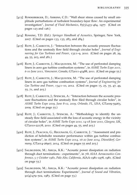
bibliography 335
[413] Ronneberger, D.; Ahrens, C.D.: “Wall shear stress caused by small am-plitude perturbations of turbulent boundary-layer flow: An experimentalinvestigation”, Journal of Fluid Mechanics, 83(3):433–464, 1977. (Cited onpages 123 and 126.)
[414] Rossing, T.D. (Ed.): Springer Handbook of Acoustics, Springer, New York,2007. (Cited on pages 133, 135, 283, and 284.)
[415] Rupp, J.; Carrotte, J.: “Interaction between the acoustic pressure fluctua-tions and the unsteady flow field through circular holes”, Journal of Engi-neering for Gas Turbines and Power, 132:1–9, 2010. (Cited on pages 28, 29,49, 55, 203, and 281.)
[416] Rupp, J.; Carrotte, J.; Macquisten, M.: “The use of perforated dampingliners in aero gas turbine combustion systems”, in ASME Turbo Expo 2011,6-10 June 2011, Vancouver, Canada, GT2011-45488, 2011. (Cited on page 55.)
[417] Rupp, J.; Carrotte, J.; Macquisten, M.: “The use of perforated dampingliners in aero gas turbine combustion systems”, Journal of Engineering forGas Turbine and Power, 134:1–10, 2012. (Cited on pages 15, 25, 35, 47, 49,55, 71, and 203.)
[418] Rupp, J.; Carrotte, J.; Spencer, A.: “Interaction between the acoustic pres-sure fluctuations and the unsteady flow filed through circular holes”, inASME Turbo Expo 2009, June 8-12, 2009, Orlando, FL, USA, GT2009-59263,2009. (Cited on page 55.)
[419] Rupp, J.; Carrotte, J.; Spencer, A.: “Methodology to identify the un-steady flow field associated with the loss of acoustic energy in the vicinityof circular holes”, in ASME Turbo Expo 2010, 14-18 June 2010, Glasgow, UK,GT2010-22178, 2010. (Cited on pages 49, 55, and 203.)
[420] Rupp, J.; Peacock, G.; Regunath, G.; Carrotte, J.: “Assessment and pre-diction of helmholtz resonator performance within gas turbine combus-tion systems”, in ASME Turbo Expo 2014, 16-20 June 2014, Düsseldorf, Ger-many, GT2014-26907, 2014. (Cited on pages 55 and 203.)
[421] Salikuddin, M.; Ahuja, K.K.: “Acoustic power dissipation on radiationthrough duct terminations - experiments”, in 7th AIAA Aeroacoustics Con-ference, 5-7 October 1981, Palo Alto, California, AIAA-1981-1978, 1981. (Citedon page 53.)
[422] Salikuddin, M.; Ahuja, K.K.: “Acoustic power dissipation on radiationthrough duct terminations: Experiments”, Journal of Sound and Vibration,91(4):479–502, 1983. (Cited on page 53.)
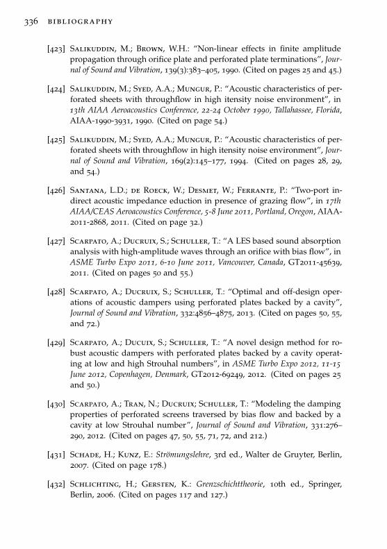
336 bibliography
[423] Salikuddin, M.; Brown, W.H.: “Non-linear effects in finite amplitudepropagation through orifice plate and perforated plate terminations”, Jour-nal of Sound and Vibration, 139(3):383–405, 1990. (Cited on pages 25 and 45.)
[424] Salikuddin, M.; Syed, A.A.; Mungur, P.: “Acoustic characteristics of per-forated sheets with throughflow in high itensity noise environment”, in13th AIAA Aeroacoustics Conference, 22-24 October 1990, Tallahassee, Florida,AIAA-1990-3931, 1990. (Cited on page 54.)
[425] Salikuddin, M.; Syed, A.A.; Mungur, P.: “Acoustic characteristics of per-forated sheets with throughflow in high itensity noise environment”, Jour-nal of Sound and Vibration, 169(2):145–177, 1994. (Cited on pages 28, 29,and 54.)
[426] Santana, L.D.; de Roeck, W.; Desmet, W.; Ferrante, P.: “Two-port in-direct acoustic impedance eduction in presence of grazing flow”, in 17thAIAA/CEAS Aeroacoustics Conference, 5-8 June 2011, Portland, Oregon, AIAA-2011-2868, 2011. (Cited on page 32.)
[427] Scarpato, A.; Ducruix, S.; Schuller, T.: “A LES based sound absorptionanalysis with high-amplitude waves through an orifice with bias flow”, inASME Turbo Expo 2011, 6-10 June 2011, Vancouver, Canada, GT2011-45639,2011. (Cited on pages 50 and 55.)
[428] Scarpato, A.; Ducruix, S.; Schuller, T.: “Optimal and off-design oper-ations of acoustic dampers using perforated plates backed by a cavity”,Journal of Sound and Vibration, 332:4856–4875, 2013. (Cited on pages 50, 55,and 72.)
[429] Scarpato, A.; Ducuix, S.; Schuller, T.: “A novel design method for ro-bust acoustic dampers with perforated plates backed by a cavity operat-ing at low and high Strouhal numbers”, in ASME Turbo Expo 2012, 11-15June 2012, Copenhagen, Denmark, GT2012-69249, 2012. (Cited on pages 25and 50.)
[430] Scarpato, A.; Tran, N.; Ducruix; Schuller, T.: “Modeling the dampingproperties of perforated screens traversed by bias flow and backed by acavity at low Strouhal number”, Journal of Sound and Vibration, 331:276–290, 2012. (Cited on pages 47, 50, 55, 71, 72, and 212.)
[431] Schade, H.; Kunz, E.: Strömungslehre, 3rd ed., Walter de Gruyter, Berlin,2007. (Cited on page 178.)
[432] Schlichting, H.; Gersten, K.: Grenzschichttheorie, 10th ed., Springer,Berlin, 2006. (Cited on pages 117 and 127.)
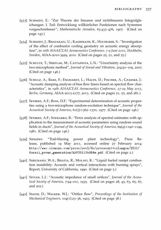
bibliography 337
[433] Schmidt, E.: “Zur Theorie der linearen und nichtlinearen Integralgle-ichungen. I. Teil: Entwicklung willkürlicher Funktionen nach Systemenvorgeschriebener”, Mathematische Annalen, 63:433–476, 1907. (Cited onpage 145.)
[434] Schmidt, J.; Bhayaraju, U.; Kashinath, K.; Hochgreb, S.: “Investigationof the effect of combustor cooling geometry on acoustic energy absorp-tion”, in 16th AIAA/CEAS Aeroacoustics Conference, 7-9 June 2010, Stockholm,Sweden, AIAA-2010-3929, 2010. (Cited on pages 25, 51, and 55.)
[435] Schultz, T.; Sheplak, M.; Cattafesta, L.N.: “Uncertainty analysis of thetwo-microphone method”, Journal of Sound and Vibration, 304:91–109, 2007.(Cited on page 146.)
[436] Schulz, A.; Bake, F.; Enghardt, L.; Haufe, D.; Fischer, A.; Czarske, J.:“Acoustic damping analysis of bias flow liners based on spectral flow char-acteristics”, in 19th AIAA/CEAS Aeroacoustics Conference, 27-29 May 2013,Berlin, Germany, AIAA-2013-2177, 2013. (Cited on pages 51, 55, and 281.)
[437] Seybert, A.F.; Ross, D.F.: “Experimental determination of acoustic proper-ties using a two-microphone random-excitation technique”, Journal of theAcoustical Society of America, 61(5):1362–1370, 1977. (Cited on page 146.)
[438] Seybert, A.F.; Soenarko, B.: “Error analysis of spectral estimates with ap-plication to the measurement of acoustic parameters using random soundfields in ducts”, Journal of the Acoustical Society of America, 69(4):1190–1199,1981. (Cited on page 146.)
[439] Siemens: “Trail-blazing power plant technology”, Press Re-lease, published 19 May 2011, accessed online 27 February 2014:http://www.siemens.com/press/pool/de/pressemitteilungen/2011/
fossil_power_generation/EFP201105064e.pdf. (Cited on page 2.)
[440] Sirignano, W.A.; Bhatia, R.; Molavi, K.: “Liquid fueled ramjet combus-tion instability: Acoustic and vortical interactions with burning sprays”,Report, University of California, 1990. (Cited on page 5.)
[441] Sivian, L.J.: “Acoustic impedance of small orifices”, Journal of the Acous-tical Society of America, 7:94–101, 1935. (Cited on pages 28, 45, 63, 65, 67,and 202.)
[442] Smith, D.; Walker, W.J.: “Orifice flow”, Proceedings of the Institution ofMechanical Engineers, 104(1):23–36, 1923. (Cited on page 38.)
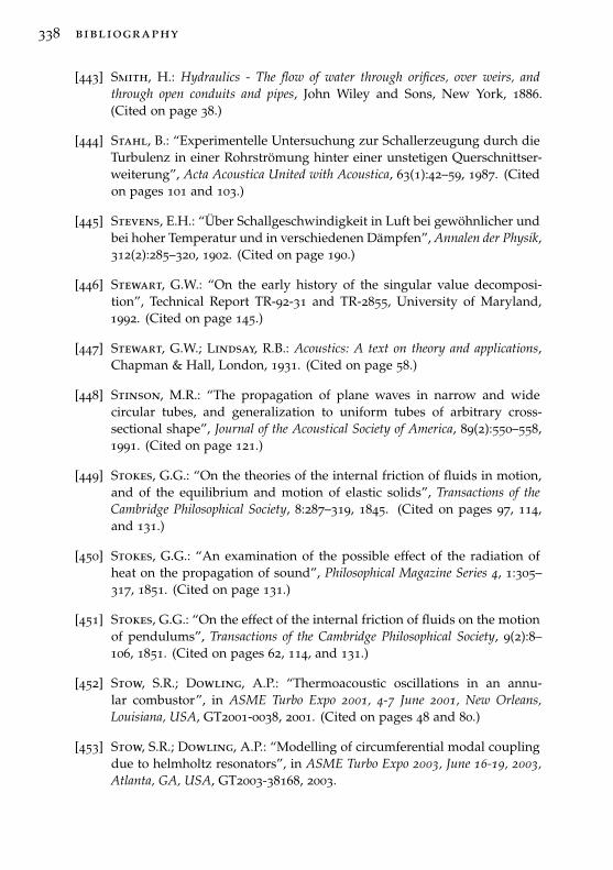
338 bibliography
[443] Smith, H.: Hydraulics - The flow of water through orifices, over weirs, andthrough open conduits and pipes, John Wiley and Sons, New York, 1886.(Cited on page 38.)
[444] Stahl, B.: “Experimentelle Untersuchung zur Schallerzeugung durch dieTurbulenz in einer Rohrströmung hinter einer unstetigen Querschnittser-weiterung”, Acta Acoustica United with Acoustica, 63(1):42–59, 1987. (Citedon pages 101 and 103.)
[445] Stevens, E.H.: “Über Schallgeschwindigkeit in Luft bei gewöhnlicher undbei hoher Temperatur und in verschiedenen Dämpfen”, Annalen der Physik,312(2):285–320, 1902. (Cited on page 190.)
[446] Stewart, G.W.: “On the early history of the singular value decomposi-tion”, Technical Report TR-92-31 and TR-2855, University of Maryland,1992. (Cited on page 145.)
[447] Stewart, G.W.; Lindsay, R.B.: Acoustics: A text on theory and applications,Chapman & Hall, London, 1931. (Cited on page 58.)
[448] Stinson, M.R.: “The propagation of plane waves in narrow and widecircular tubes, and generalization to uniform tubes of arbitrary cross-sectional shape”, Journal of the Acoustical Society of America, 89(2):550–558,1991. (Cited on page 121.)
[449] Stokes, G.G.: “On the theories of the internal friction of fluids in motion,and of the equilibrium and motion of elastic solids”, Transactions of theCambridge Philosophical Society, 8:287–319, 1845. (Cited on pages 97, 114,and 131.)
[450] Stokes, G.G.: “An examination of the possible effect of the radiation ofheat on the propagation of sound”, Philosophical Magazine Series 4, 1:305–317, 1851. (Cited on page 131.)
[451] Stokes, G.G.: “On the effect of the internal friction of fluids on the motionof pendulums”, Transactions of the Cambridge Philosophical Society, 9(2):8–106, 1851. (Cited on pages 62, 114, and 131.)
[452] Stow, S.R.; Dowling, A.P.: “Thermoacoustic oscillations in an annu-lar combustor”, in ASME Turbo Expo 2001, 4-7 June 2001, New Orleans,Louisiana, USA, GT2001-0038, 2001. (Cited on pages 48 and 80.)
[453] Stow, S.R.; Dowling, A.P.: “Modelling of circumferential modal couplingdue to helmholtz resonators”, in ASME Turbo Expo 2003, June 16-19, 2003,Atlanta, GA, USA, GT2003-38168, 2003.
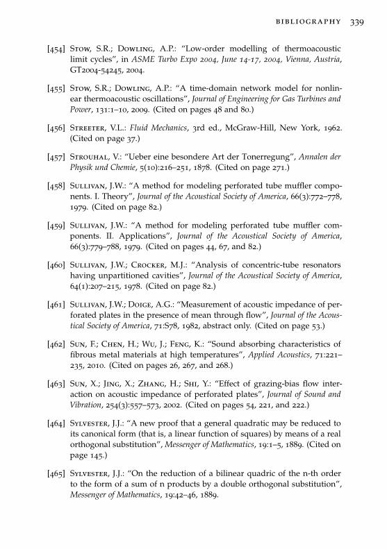
bibliography 339
[454] Stow, S.R.; Dowling, A.P.: “Low-order modelling of thermoacousticlimit cycles”, in ASME Turbo Expo 2004, June 14-17, 2004, Vienna, Austria,GT2004-54245, 2004.
[455] Stow, S.R.; Dowling, A.P.: “A time-domain network model for nonlin-ear thermoacoustic oscillations”, Journal of Engineering for Gas Turbines andPower, 131:1–10, 2009. (Cited on pages 48 and 80.)
[456] Streeter, V.L.: Fluid Mechanics, 3rd ed., McGraw-Hill, New York, 1962.(Cited on page 37.)
[457] Strouhal, V.: “Ueber eine besondere Art der Tonerregung”, Annalen derPhysik und Chemie, 5(10):216–251, 1878. (Cited on page 271.)
[458] Sullivan, J.W.: “A method for modeling perforated tube muffler compo-nents. I. Theory”, Journal of the Acoustical Society of America, 66(3):772–778,1979. (Cited on page 82.)
[459] Sullivan, J.W.: “A method for modeling perforated tube muffler com-ponents. II. Applications”, Journal of the Acoustical Society of America,66(3):779–788, 1979. (Cited on pages 44, 67, and 82.)
[460] Sullivan, J.W.; Crocker, M.J.: “Analysis of concentric-tube resonatorshaving unpartitioned cavities”, Journal of the Acoustical Society of America,64(1):207–215, 1978. (Cited on page 82.)
[461] Sullivan, J.W.; Doige, A.G.: “Measurement of acoustic impedance of per-forated plates in the presence of mean through flow”, Journal of the Acous-tical Society of America, 71:S78, 1982, abstract only. (Cited on page 53.)
[462] Sun, F.; Chen, H.; Wu, J.; Feng, K.: “Sound absorbing characteristics offibrous metal materials at high temperatures”, Applied Acoustics, 71:221–235, 2010. (Cited on pages 26, 267, and 268.)
[463] Sun, X.; Jing, X.; Zhang, H.; Shi, Y.: “Effect of grazing-bias flow inter-action on acoustic impedance of perforated plates”, Journal of Sound andVibration, 254(3):557–573, 2002. (Cited on pages 54, 221, and 222.)
[464] Sylvester, J.J.: “A new proof that a general quadratic may be reduced toits canonical form (that is, a linear function of squares) by means of a realorthogonal substitution”, Messenger of Mathematics, 19:1–5, 1889. (Cited onpage 145.)
[465] Sylvester, J.J.: “On the reduction of a bilinear quadric of the n-th orderto the form of a sum of n products by a double orthogonal substitution”,Messenger of Mathematics, 19:42–46, 1889.
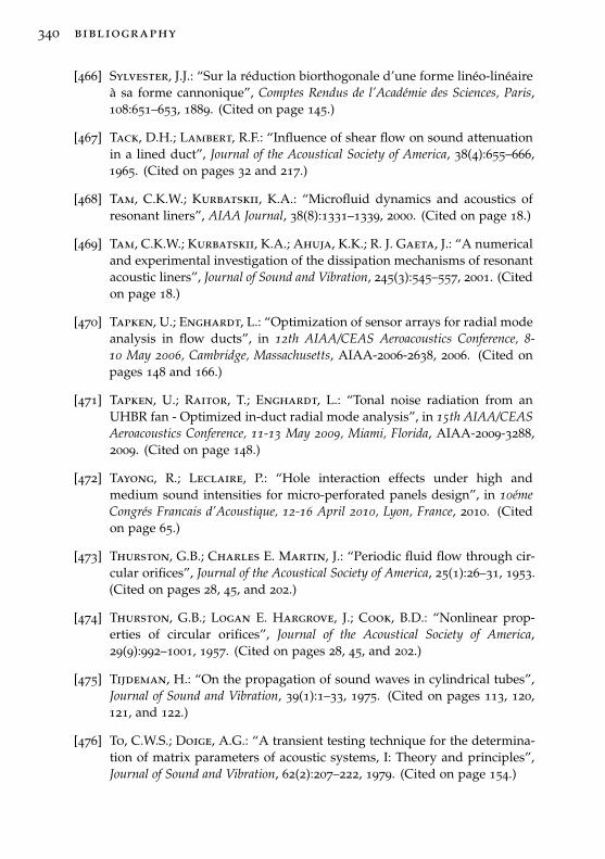
340 bibliography
[466] Sylvester, J.J.: “Sur la réduction biorthogonale d’une forme linéo-linéaireà sa forme cannonique”, Comptes Rendus de l’Académie des Sciences, Paris,108:651–653, 1889. (Cited on page 145.)
[467] Tack, D.H.; Lambert, R.F.: “Influence of shear flow on sound attenuationin a lined duct”, Journal of the Acoustical Society of America, 38(4):655–666,1965. (Cited on pages 32 and 217.)
[468] Tam, C.K.W.; Kurbatskii, K.A.: “Microfluid dynamics and acoustics ofresonant liners”, AIAA Journal, 38(8):1331–1339, 2000. (Cited on page 18.)
[469] Tam, C.K.W.; Kurbatskii, K.A.; Ahuja, K.K.; R. J. Gaeta, J.: “A numericaland experimental investigation of the dissipation mechanisms of resonantacoustic liners”, Journal of Sound and Vibration, 245(3):545–557, 2001. (Citedon page 18.)
[470] Tapken, U.; Enghardt, L.: “Optimization of sensor arrays for radial modeanalysis in flow ducts”, in 12th AIAA/CEAS Aeroacoustics Conference, 8-10 May 2006, Cambridge, Massachusetts, AIAA-2006-2638, 2006. (Cited onpages 148 and 166.)
[471] Tapken, U.; Raitor, T.; Enghardt, L.: “Tonal noise radiation from anUHBR fan - Optimized in-duct radial mode analysis”, in 15th AIAA/CEASAeroacoustics Conference, 11-13 May 2009, Miami, Florida, AIAA-2009-3288,2009. (Cited on page 148.)
[472] Tayong, R.; Leclaire, P.: “Hole interaction effects under high andmedium sound intensities for micro-perforated panels design”, in 10émeCongrés Francais d’Acoustique, 12-16 April 2010, Lyon, France, 2010. (Citedon page 65.)
[473] Thurston, G.B.; Charles E. Martin, J.: “Periodic fluid flow through cir-cular orifices”, Journal of the Acoustical Society of America, 25(1):26–31, 1953.(Cited on pages 28, 45, and 202.)
[474] Thurston, G.B.; Logan E. Hargrove, J.; Cook, B.D.: “Nonlinear prop-erties of circular orifices”, Journal of the Acoustical Society of America,29(9):992–1001, 1957. (Cited on pages 28, 45, and 202.)
[475] Tijdeman, H.: “On the propagation of sound waves in cylindrical tubes”,Journal of Sound and Vibration, 39(1):1–33, 1975. (Cited on pages 113, 120,121, and 122.)
[476] To, C.W.S.; Doige, A.G.: “A transient testing technique for the determina-tion of matrix parameters of acoustic systems, I: Theory and principles”,Journal of Sound and Vibration, 62(2):207–222, 1979. (Cited on page 154.)
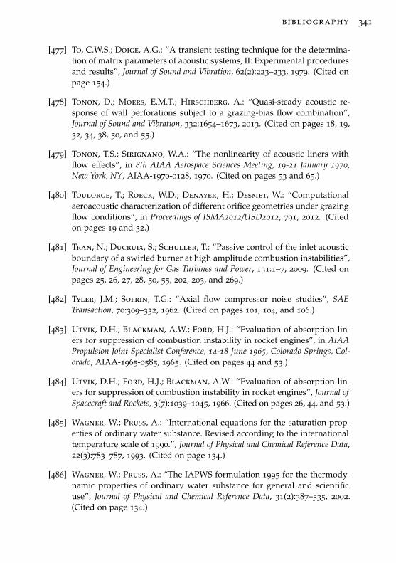
bibliography 341
[477] To, C.W.S.; Doige, A.G.: “A transient testing technique for the determina-tion of matrix parameters of acoustic systems, II: Experimental proceduresand results”, Journal of Sound and Vibration, 62(2):223–233, 1979. (Cited onpage 154.)
[478] Tonon, D.; Moers, E.M.T.; Hirschberg, A.: “Quasi-steady acoustic re-sponse of wall perforations subject to a grazing-bias flow combination”,Journal of Sound and Vibration, 332:1654–1673, 2013. (Cited on pages 18, 19,32, 34, 38, 50, and 55.)
[479] Tonon, T.S.; Sirignano, W.A.: “The nonlinearity of acoustic liners withflow effects”, in 8th AIAA Aerospace Sciences Meeting, 19-21 January 1970,New York, NY, AIAA-1970-0128, 1970. (Cited on pages 53 and 65.)
[480] Toulorge, T.; Roeck, W.D.; Denayer, H.; Desmet, W.: “Computationalaeroacoustic characterization of different orifice geometries under grazingflow conditions”, in Proceedings of ISMA2012/USD2012, 791, 2012. (Citedon pages 19 and 32.)
[481] Tran, N.; Ducruix, S.; Schuller, T.: “Passive control of the inlet acousticboundary of a swirled burner at high amplitude combustion instabilities”,Journal of Engineering for Gas Turbines and Power, 131:1–7, 2009. (Cited onpages 25, 26, 27, 28, 50, 55, 202, 203, and 269.)
[482] Tyler, J.M.; Sofrin, T.G.: “Axial flow compressor noise studies”, SAETransaction, 70:309–332, 1962. (Cited on pages 101, 104, and 106.)
[483] Utvik, D.H.; Blackman, A.W.; Ford, H.J.: “Evaluation of absorption lin-ers for suppression of combustion instability in rocket engines”, in AIAAPropulsion Joint Specialist Conference, 14-18 June 1965, Colorado Springs, Col-orado, AIAA-1965-0585, 1965. (Cited on pages 44 and 53.)
[484] Utvik, D.H.; Ford, H.J.; Blackman, A.W.: “Evaluation of absorption lin-ers for suppression of combustion instability in rocket engines”, Journal ofSpacecraft and Rockets, 3(7):1039–1045, 1966. (Cited on pages 26, 44, and 53.)
[485] Wagner, W.; Pruss, A.: “International equations for the saturation prop-erties of ordinary water substance. Revised according to the internationaltemperature scale of 1990.”, Journal of Physical and Chemical Reference Data,22(3):783–787, 1993. (Cited on page 134.)
[486] Wagner, W.; Pruss, A.: “The IAPWS formulation 1995 for the thermody-namic properties of ordinary water substance for general and scientificuse”, Journal of Physical and Chemical Reference Data, 31(2):387–535, 2002.(Cited on page 134.)
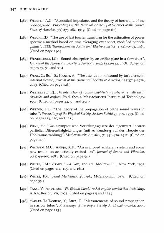
342 bibliography
[487] Webster, A.G.: “Acoustical impedance and the theory of horns and of thephonograph”, Proceedings of the National Academy of Sciences of the UnitedStates of America, 5(7):275–282, 1919. (Cited on page 60.)
[488] Welch, P.D.: “The use of fast fourier transform for the estimation of powerspectra: a method based on time averaging over short, modified periodi-grams”, IEEE Transactions on Audio and Electroacoustics, 15(2):70–73, 1967.(Cited on page 140.)
[489] Wendoloski, J.C.: “Sound absorption by an orifice plate in a flow duct”,Journal of the Acoustical Society of America, 104(1):122–132, 1998. (Cited onpages 47, 54, and 71.)
[490] Weng, C.; Boij, S.; Hanifi, A.: “The attenuation of sound by turbulence ininternal flows”, Journal of the Acoustical Society of America, 133:3764–3776,2013. (Cited on page 126.)
[491] Westervelt, P.J.: The interaction of a finite amplitude acoustic wave with smallobstacles and orifices, Ph.d. thesis, Massachusetts Institute of Technology,1951. (Cited on pages 44, 53, and 251.)
[492] Weston, D.E.: “The theory of the propagation of plane sound waves intubes”, Proceedings of the Physical Society, Section B, 66:695–709, 1953. (Citedon pages 113, 120, and 121.)
[493] Weyl, H.: “Das asymptotische Verteilungsgesetz der eigenwert linearerpartieller Differentialgleichungen (mit Anwendung auf der Theorie derHohlraumstrahlung)”, Mathematische Annalen, 71:441–479, 1912. (Cited onpage 145.)
[494] Whiffen, M.C.; Ahuja, K.K.: “An improved schlieren system and somenew results on acoustically excited jets”, Journal of Sound and Vibration,86(1):99–105, 1983. (Cited on page 54.)
[495] White, F.M.: Viscous Fluid Flow, 2nd ed., McGraw-Hill, New York, 1991.(Cited on pages 114, 115, and 161.)
[496] White, F.M.: Fluid Mechanics, 4th ed., McGraw-Hill, 1998. (Cited onpage 33.)
[497] Yang, V.; Anderson, W. (Eds.): Liquid rocket engine combustion instability,AIAA, Reston, VA, 1995. (Cited on pages 5 and 323.)
[498] Yazaki, T.; Tashiro, Y.; Biwa, T.: “Measurements of sound propagationin narrow tubes”, Proceedings of the Royal Society A, 463:2855–2862, 2007.(Cited on page 113.)
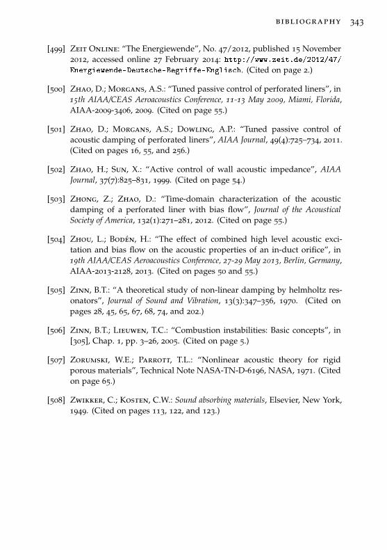
bibliography 343
[499] Zeit Online: “The Energiewende”, No. 47/2012, published 15 November2012, accessed online 27 February 2014: http://www.zeit.de/2012/47/Energiewende-Deutsche-Begriffe-Englisch. (Cited on page 2.)
[500] Zhao, D.; Morgans, A.S.: “Tuned passive control of perforated liners”, in15th AIAA/CEAS Aeroacoustics Conference, 11-13 May 2009, Miami, Florida,AIAA-2009-3406, 2009. (Cited on page 55.)
[501] Zhao, D.; Morgans, A.S.; Dowling, A.P.: “Tuned passive control ofacoustic damping of perforated liners”, AIAA Journal, 49(4):725–734, 2011.(Cited on pages 16, 55, and 256.)
[502] Zhao, H.; Sun, X.: “Active control of wall acoustic impedance”, AIAAJournal, 37(7):825–831, 1999. (Cited on page 54.)
[503] Zhong, Z.; Zhao, D.: “Time-domain characterization of the acousticdamping of a perforated liner with bias flow”, Journal of the AcousticalSociety of America, 132(1):271–281, 2012. (Cited on page 55.)
[504] Zhou, L.; Bodén, H.: “The effect of combined high level acoustic exci-tation and bias flow on the acoustic properties of an in-duct orifice”, in19th AIAA/CEAS Aeroacoustics Conference, 27-29 May 2013, Berlin, Germany,AIAA-2013-2128, 2013. (Cited on pages 50 and 55.)
[505] Zinn, B.T.: “A theoretical study of non-linear damping by helmholtz res-onators”, Journal of Sound and Vibration, 13(3):347–356, 1970. (Cited onpages 28, 45, 65, 67, 68, 74, and 202.)
[506] Zinn, B.T.; Lieuwen, T.C.: “Combustion instabilities: Basic concepts”, in[305], Chap. 1, pp. 3–26, 2005. (Cited on page 5.)
[507] Zorumski, W.E.; Parrott, T.L.: “Nonlinear acoustic theory for rigidporous materials”, Technical Note NASA-TN-D-6196, NASA, 1971. (Citedon page 65.)
[508] Zwikker, C.; Kosten, C.W.: Sound absorbing materials, Elsevier, New York,1949. (Cited on pages 113, 122, and 123.)