Acoustic monitoring of photopolymerization in UV curable coatings · 2016-05-18 · Acoustic monitoring of photopolymerization in UV curable coatings Dissertation zur Erlangung des

Acoustic monitoring of photopolymerization

in UV curable coatings

Dissertation zur Erlangung des Doktorgrades der

mathematisch-naturwissenschaftlichen Fakultät der Universität Augsburg vorgelegt von

Elena Magdalena De Ambroggi

Lehrstuhl für Experimentalphysik I Institut für Physik

Universität Augsburg

Erster Gutachter: Prof. Dr. Achim Wixforth Zweiter Gutachter: Prof. Dr. Armin Reller Tag der mündlichen Prüfung: 21.07.2011

Acknowledgements

First of all I would like to thank my supervisor, Prof. Dr. Achim Wixforth at the

University Augsburg, Physics Department for his supportive advice and his technical

steering during this project.

Further, I would to thanks to Dr. Andreas Hörner for his technical support and for

development of the FFT analysis program.

To the firm Manroland and in particular to Mr. Thomas Walther and Mr. Hartmut

Hübner, I am grateful for giving me the opportunity to work on the “Nanocure” project.

Here, I would like to thanks to Dr. Ralph Klarmann for introducing me at University

Augsburg and give rise to this work.

I would like to thanks to Rolf Anders for the technical support in all questions

regarding Linux, the help in programming and for being a friend in good and bad

times.

For the FTIR spectroscopy measurements thank you to Dr. Tom Scherzer (IOM

Leipzig), Dr. Petra Herbert-Engel (INM Saarbrücken), Dr. Alexej Pashkin, Dr.

Leonetta Baldassare and Dr. Sindu Louis (ex alumni Experimental Physik II).

For the ESR spectroscopy thanks to Dr. Wolfgang Knolle (IOM Leipzig) and to Dr.

Hans Albrecht Krug von Nidda (Experimental Physik V, Universität Augsburg).

Many thanks to the technical staff of Experimental Physik I: Olga Ustinov, Sidonie

Lieber, Andreas Spörhase and Alex Hupfner for all the help in all the handicraft work

and more.

Thank you to my collegues, in particular Christoph Westernhausen, Marcin Malecha

and Dr. Stefan Völk as well either for the physics discussions as for the small talks.

Last but not least, I would like to thank my family who supported me throughout this

work. In particular, I would like to thanks to my loving sons and to excuse me not

being every time disposable for them. Thank you to my husband for giving me

support and love in a difficult time for both of us.

- 1 -

Motivation and Objectives……………………………………………………………….11 Chapter 1

1. UV Coatings…………………………………………………………………………… 14

1.1 Absorption of light....................................................................................... 14

1.2 Basic Principles of polymerization .............................................................. 17

1.2.1 Photoinitiated radical polymerisation .............................................................. 17

1.2.2 Acrylate systems............................................................................................. 21

1.2.3 Photoinitiated cationic polymerisation............................................................. 23

1.3 Photoinitiators............................................................................................. 24

1.4 Factors affecting the degree of cure........................................................... 28

1.4.1 Oxygen inhibition ............................................................................................ 28

1.4.2 Influence of the sample temperature .............................................................. 29

1.4.3 Influence of the monomer viscosity................................................................. 29

1.4.4 Influence of the film thickness......................................................................... 29

1.4.5 Factors affecting the degree of cure in Acrylate Systems............................... 30

Chapter 2

2. Mechanical oscillation and waves theory 30

2.1. Introduction 30

2.2. Basic motion: The simple harmonic oscillator 32

2.3. Energy of vibration 34

2.4. Vibration of a plane surface 36

2.5. The wave equation for a stretched membrane 36

2.6. The vibrating circular membrane with fixed rim 37

2.7. Finite Element Simulation for a vibrating membrane 40

2.8. Analytical Models 40

2.8.1. Circular membrane with fixed rim [86] 40

2.1.1. Multi-Layer Circular Membrane with Fixed Rim [86]. 42

2.1.2. Finite Element Models 43

- 2 -

2.1.3. Simulation Results 44

Chapter 3

3. Standard techniques for investigation of the photopolymerization .................. 48

3.1. FTIR and Real Time FTIR Spectroscopy........................................................ 48

3.1.1. Rotational energy states ................................................................................. 49

3.1.2. Vibrational energy states ................................................................................ 50

3.1.3. Optical transition and IR absorption................................................................ 51

3.1.4. The Lambert-Beer law .................................................................................... 51

3.1.5. Snell’s law....................................................................................................... 52

3.1.6. Fresnel equation ............................................................................................. 53

3.2. FTIR measurements ....................................................................................... 54

3.2.1. Experimental Data .......................................................................................... 54

3.3. Differential Scanning Calorimetry (DSC) ........................................................ 59

3.4. Electron paramagnetic resonance (EPR) ....................................................... 64

3.5. Magnetic resonance and chemical bonds....................................................... 69

3.6. Detection and interpretation of an ESR signal ................................................ 69

3.7. Anisotropy of the ESR signal .......................................................................... 70

3.8. Experimental................................................................................................... 71

3.9. Atomic force microscopy (AFM)...................................................................... 75

3.10. Adhesion......................................................................................................... 79

3.11. Substrat wetting .............................................................................................. 79

3.12. Film shrinkage ................................................................................................ 79

3.13. Rheometrical measurements .......................................................................... 81

Chapter 4

4. Experimental Technique for UV-curable coatings and clear coatings………….. 85

4.1. Acoustic Resonator………………………………………………………………….. 85

4.1.3. Acoustic Vibration Detection System .............................................................. 90

4.2. The Damped, Freely Vibration mode (time domain experiment)..................... 91

- 3 -

4.3. The forced vibration Mode (frequency domain experiment)............................ 93

4.3.1. Forced Oscillation equations........................................................................... 93

4.3.1.1. Correlation to a two dimensional case (Circular Membrane). ...................... 95

4.4. Vibration modes of the circular, fixed membrane…………………………………. 96

4.4.1. Experimental................................................................................................... 99

4.4.2. Analysis of vibration using Fourier’s Theorem [22, 23, 24, 88] 101

4.4.3. Experimental The Fast Fourier Transform (FFT) .......................................... 103

4.4.4. Frequency Analysis using Fast Fourier Transformation FFT Software 104

4.5. UV lamp……………………………………………………………………………….110

4.6. Sample preparation…………………………………………………………………. 113

4.6.1. Substrate ...................................................................................................... 113

4.6.2. Method of application.................................................................................... 113

4.6.3. Sample formulation....................................................................................... 115

4.7. Measurements in the frequency domain 116

4.7.1. Measurements of pigmented coatings on paper substrate ........................... 116

4.7.2. Paper irradiation ........................................................................................... 123

4.7.3. Plastics substrate.......................................................................................... 124

4.7.4. Mass loss...................................................................................................... 125

4.8. Measurements performed on samples printed by a MAN Roland printing machine.................................................................................................................. 127

4.9. Measurements in the time domain................................................................ 131

Chapter 5

5. SAW Sensor ................................................................................................. 136

5.1. Introduction................................................................................................... 136

5.1.1. Piezoelectric Substrate Materials.................................................................. 137

5.1.2. Fabrication of Acoustic Wave Devices.......................................................... 140

5.1.3. Acoustic Wave Sensors................................................................................ 141

5.1.4. BAW sensor.................................................................................................. 141

- 4 -

5.1.5. Surface Acoustic Wave Sensor .................................................................... 144

5.1.6. Acoustic Waves in a solid ............................................................................. 145

5.1.7. Acoustic waves propagation in solids ........................................................... 146

5.1.8. Excitation of surface acoustic waves ............................................................ 149

5.1.9. Sensor devices operating with Rayleigh Waves (SAW Sensor) ................... 150

5.1.10. Factors affecting measurements signal of a surface acoustic wave sensor 154

5.2. Experimental................................................................................................. 162

5.2.1. Sample preparation ...................................................................................... 163

5.2.2. SAW Sensor ................................................................................................. 164

5.2.3. Estimation of the SAW amplitude and damping from the transmission measurements........................................................................................................ 165

5.2.4. Measurements on pigmented coatings ......................................................... 166

5.2.5. Measurements on clear coatings .................................................................. 170

Chapter 6

6. Dynamic Mechanical Analysis ...................................................................... 176

6.1. Basic principles............................................................................................. 176

6.2. Start of the polymerization ............................................................................ 182

6.3. Gelation ........................................................................................................ 183

6.4. Vitrification .................................................................................................... 183

6.5. Stress development ...................................................................................... 183

6.6. Determination of the elastic modulus of an acrylate sample under UV irradiation................................................................................................................ 184

Chapter 7

7 Conclusions…………………………………………………………………………..188

7.1. The acoustic resonator measurements……………………………………………188

7.1.1. Paper Substrate……………………………………………………………..........189

7.1.2. Plastic Substrates…………………………………………………………………191

7.1.3. Summary…………………………………………………………………………...191

7.2. The SAW sensor measurements…………………………………………………..193

- 5 -

List of Figures:

Fig.1. 1: Schema [2] of a photoinduced polymerization reaction. ............................................................... 15

Fig.1. 2: The n and π bonding orbitals present in a carbonyl group [83] ................................................... 16

Fig.1. 3: Geometries of the carbonyl group; the oxygen has two pairs of unshared electrons. [83] ...... 16

Fig.1. 4: Absorption spectrum of benzophenone. [84] .................................................................................. 17

Fig.1. 5: Jablonski diagram. [84] ...................................................................................................................... 17

Fig.1. 6: Schematic diagram of a photoinitiated polymerization reaction [85]. .......................................... 18

Fig.1. 7: Schematic representation of photoinitiated radical polymerization [1]. ....................................... 20

Fig.1. 8: Termination reaction through combination of two reactive species to a stable radical [85]..... 21

Fig.1. 9:Termination reaction through disproportionation of the hydrogen atom moved to form a stable radical. [85] .......................................................................................................................................................... 21

Fig.1. 10: Photoinitiated crosslinking polymerisation of a diacrylate monomer [2]. .................................. 23

Fig.1. 11: Different types of acrylate compounds used in the coating industry [2] ................................... 24

Fig.1. 12: Polymerization of isobutylene [85]. ................................................................................................ 25

Fig.1. 13: α and β cleavage reaction [3].......................................................................................................... 26

Fig.1. 14: Photoinitiators species of type II [68]. ............................................................................................ 26

Fig.1. 15: The benzophenon triplet is deactivated by energy transfer to oxygen [68]. ............................ 27

Fig.1. 16: Reaction of triplet benzophenone with an amine synergist. ....................................................... 27

Fig.1. 17: The photochemical splitting of BDK (benzil dimethyl ketal) [75]................................................ 28

Fig.1. 18: Absorption spectra of benzophenone. ........................................................................................... 28

Fig.1. 19: Oxygen reacts with hydrogen atoms from the polymer chain forming hydroperoxides. ........ 30

Fig.2.1 Propagation of a sound wave.................................................................................................... 31

Fig.2.2 Transverse wave on a string; the displacement of the medium is perpendicular to the direction of propagation of the wave .................................................................................................................... 31

Fig.2.3 Longitudinal Wave Propagation (Top) and Transversal Wave Propagation (Bottom) .............. 32

Fig.2.4 Simple harmonic Oscillator........................................................................................................ 33

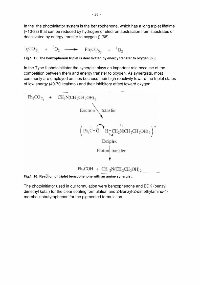
Fig.2.5: Circular Membrane Modes [98] ................................................................................................ 39

Fig.2.6 The four lowest vibrational modes for a circular membrane [98] .............................................. 39

Fig.2.7: Vibrating membrane mesh ....................................................................................................... 44

Fig.2.8: Simulation model for a two layer vibrating membrane ............................................................. 45

Fig.2.9: Increasing of the eigenfrequencies for a two layer model with increasing cure time (no alteration of paper occurs)..................................................................................................................... 45

- 6 -

Fig.2.10: Decrease of the eigenfrequencies for a two layer model with increasing cure time (paper altering matches’ experimental data) .................................................................................................... 46

Fig.3. 1: Refraction of light at the interface of two media of different refractive indices. [92]................ 53

Fig.3. 2: Schematic of an irradiated sample on the ATR crystal in a FTIR Spectrometer [91] ............. 55

Fig.3. 3: Concentration of the double bond of an acrylate sample........................................................ 56

Fig.3. 4: The decrease in the double bond band (CH=CH2) of the functional group indicates the degree of polymerization. .................................................................................................................................. 56

Fig.3.5: Polymerization profiles recorded by RTIR spectroscopy for a sample exposed to UV light under different atmospheres.................................................................................................................. 57

Fig.3. 6: Degree of conversion of the functional group in a clear (squares) and three pigmented acrylate formulation: yellow (x), magenta (◊), cyan (+). ........................................................................ 58

Fig.3.7: Schema of a DSC (differential scanning calorimeter) [92] ....................................................... 59

Fig.3.8: Typically isothermal curve of a sample obtained with DSC analysis ....................................... 60

Fig.3.9: In-situ measurement of a clear and pigmented coating. The clear coating exhibits the higher degree of conversion; the second one is the yellow pigmented coating, follows by the black and blue pigmented coating. ................................................................................................................................ 61

Fig.3.10: Thermogram of a clear coating (black) and pigmented coatings. The clear coating reaches the higher degree of conversion; meanwhile the black pigmented coating exhibits the lower degree of conversion. ............................................................................................................................................ 62

Fig.3. 11: Overview of the principle interactions and their range in the EPR spectroscopy. [89] ......... 65

Fig.3. 12: Orientation of unpaired electrons in a static magnetic field. [89] .......................................... 66

Fig.3. 13: Energy splitting of an electron in presence of a magnetic field [93]...................................... 66

Fig.3. 14: Schematic of the ESR resonator. [89] ................................................................................... 67

Fig.3. 15: The differential scan of the absorption spectrum gives, because of the modulation of the magnetic field strength, the original ESR spectrum (I-derivative of the absorption spectrum). A: absorption spectrum of the microwave radiation; B: Original ESR spectrum. [89] ............................... 68

Fig.3. 16: The resonance condition by energy splitting. [89]................................................................. 68

Fig.3. 17: A cyan pigmented formulation before (black line) and after curing (red line)........................ 72

Fig.3. 18: A yellow pigmented formulation before (black line) and after curing (red line) ..................... 73

Fig.3. 19: A magenta pigmented formulation before (black line) and after curing (red line) ................. 73

Fig.3. 20: Dynamic of the radicals concentration in a magenta pigmented formulation recorded over five days................................................................................................................................................. 74

Fig.3. 21: Diagram of the measurement principle of AFM.................................................................... 75

Fig.3. 22: Schema of the measurement procedure with AFM [90]........................................................ 76

Fig.3. 23: The cantilever tip penetrates 10nm depth in the sample; the removing force is FX=125 nN. 77

Fig.3. 24: Topography of a UV coating on a paper substrate ............................................................... 78

- 7 -

Fig.3.25: Bad adhesion of a urethane acrylate coating on a PVC substrate ........................................ 80

Fig.3.26: Good adhesion of a urethane acrylate coating applied to a PVC substrate .......................... 80

Fig.3. 27: Haake Mars thermo rheometer for characterization of polymers.......................................... 81

Fig.3. 28: Oscillating Plate Rheometer.................................................................................................. 83

Fig.3.29: Viscosity decrease in a urethane acrylate sample with increase of temperature. ................. 84

Fig.4.1: Schematic diagram of the set-up arrangement a) Frequency and b) Time Domain 86

Fig.4.2: Schematic diagram of the optical detection unit 87

Fig.4. 3: Acoustic Resonator with sample clamp 88

Fig.4. 4: The tension of the membrane can be increase by acting the device containing the loudspeaker. 88

Fig.4. 5: Optical receiver unit 89

Fig.4. 6: Photo of the receiver unit 90

Fig.4. 7: The first six vibration modes of a round membrane [93]. 97

Fig.4.8: The first experimentally measured vibration modes of the paper membrane. 98

Fig.4.9: The Fourier series of a square wave vibration of unit amplitude and period T. 102

In Fig.4.9 we see the result retaining various numbers of terms of the series. Because of the discontinuities, the Fourier series develops visible overshoot near these times if a large enough number of terms are retained [22, 88]. 103

Fig.4. 10: Sample tensed between the two plates of the clamp. The tension on the sample can be increase by pulling the round device forward. 104

Fig.4. 11: Recorded amplitude scan of the membrane after a short an intense pulse like excitation. The oscilloscope was set at 1 ms time window. 105

Fig.4.12: Photo of the LabView front panel, corresponding to the oscilloscope data as per Fig.4.11. 106

Fig.4. 13: The block diagram for the Lab View program 107

Fig.4.14: UV Scan Tesa from Honle. The UV dose is given from the evaluation of change in the colour of the TESA strips. 111

Fig.4.15: Doses of UV light as function of distance-substrate. 111

Fig.4.16: Absorption spectrum of HPA Phillips 400W UV lamp 112

Fig.4.17: Front of the UV lamp protection box with the longitudinal removable shutter. 112

Fig.4.18: Metal plate with paint roller 114

Fig.4.19: Photo of the sample preparation set-up: metal plate and through the power generator controlled paint roller 114

Fig.4.20: Frontal photo of the paint roller 115

- 8 -

Fig.4.21: Changes in the frequency response with increase of the cure time by a yellow pigmented sample. 117

Fig.4.22: Frequency decrease in a yellow pigmented sample. 118

Fig.4.23: Changes in the resonant frequency for a black pigmented sample. 118

Fig.4.24: Frequency decrease in a black pigmented sample. 119

Fig.4.25: Changes in the resonant frequency for magenta magenta pigmented sample. 120

Fig.4.26: Frequency decrease in a magenta pigmented sample. 120

Fig.4.27: Changes in the resonant frequency for a cyan pigmented sample. 121

Fig.4.28: Frequency decrease in a cyan pigmented sample. 122

Fig.4.29: Changes in the resonant frequency of an irradiated blank paper sample. 123

Fig.4.30: Changes in the resonant frequency with increase of the irradiation time. 124

Fig.4.31: Changes in the resonance frequency for a sample coated on plastic substrate (PVC). 125

Fig.4.32: Mass decrease with increase cure time in the paper membrane. 126

Fig.4. 33: Printing procedure in an MAN Roland printing machine. The coated sheets are exposed at four UV operations (one for each pigmentation) and an additionally one for the clear coating on the top. 127

Fig.4. 34: Changes in the resonance frequency of samples printed in a Man Roland printed machine. Only very little change of the resonance frequency could be detected, whereas a prominent change in the line shape and –integral is clearly seen. 128

Fig.4.35: Changes in the resonance frequency of a clear coating printed on Luxo Magic paper. 129

Fig.4.36: Changes in the resonance frequency for a magenta pigmented sample. 130

Fig.4.37: Changes in the resonance frequency of a magenta and yellow pigmented sample 130

Fig.4.38: Dynamics of the drying process in a solvent based coating on a paper substrate. The resonance frequency of the system decreases after applying the coating and, with the start of the drying process, the frequency begins to increase again until a constant value is reached. 132

Fig.4. 39: Dynamic of the drying process in a solvent based coating on an aluminium substrate. The resonance frequency increases from a minimum of 1700 Hz to a maximum of 2700 Hz corresponding to a final steady state. 133

Fig.5.1: The cells structure by quartz and the piezoelectric effect… ……………………………………136

Fig.5.2: Photo of a quartz crystal and the different possible cuts........................................................ 138

Fig.5.3: Photolithographic process for manufacturing of acoustic wave devices................................ 140

Fig.5.4: Typical configuration of an acoustic wave sensor.................................................................. 141

Fig.5.5: Schema of a quartz crystal sensor. ........................................................................................ 142

Fig.5.6: Attenuation of an acoustic wave by propagation into fluids. The attenuation is due to the fluid viscosity. .............................................................................................................................................. 144

Fig.5.7: The stress tensor, in the coordinates system......................................................................... 147

- 9 -

Fig.5.8: The Rayleigh wave consists of a longitudinal and a perpendicular to the direction of propagation component....................................................................................................................... 149

Fig.5.9: Rayleigh waves surface propagation and the elliptical trajectory of the moved particles. ..... 149

Fig.5.10: Sketch of a SAW transducer on a piezoelectric substrate. .................................................. 150

Fig.5.11:The delay line configuration in a SAW sensor ...................................................................... 152

Fig.5.12: Surface acoustic wave sensor components: one port resonator (left) and two port resonator (right). .................................................................................................................................................. 152

Fig.5.14: Frequency shift as function of temperature for quartz oscillators for different cuts. ............ 156

Fig.5.15: Shear deformation in a solid................................................................................................. 157

Fig.5.16: Deformation of an: a) acoustically thin film and b) acoustically thick film, by the propagation of a Rayleigh wave. ............................................................................................................................. 158

Fig.5.17: The SAW induces a deformation in a) an acoustically thin coating film, b) acoustically thick coating film deposed onto the LiNbO3 substrate. ............................................................................... 159

Fig.5.18: Damping behaviour as function of the film thickness for a coating film. The model represents a thin coating film................................................................................................................................. 161

Fig.5.19: Damping behaviour as function of the film thickness for a coating film. The model represented a thin acrylate coating film............................................................................................... 162

Fig.5.20: Spin-coating bowl for sample preparation. ........................................................................... 163

Fig.5.21:The chip bonded on a sample holder. ................................................................................... 164

Fig.5.22: Photo of a sample on the chip.............................................................................................. 164

Fig.5.23: Schema of the set-up for transmission measurements........................................................ 165

Fig.5.24: The UV coatings were printed on a polypropylene layer. The coated side was pressed onto the SAW sensor and positioned between the two IDT’s. S................................................................. 167

Fig.5.25: Magenta samples on thin polypropylene foil irradiated through the substrate..................... 167

Fig.5.26: Yellow sample on thin polypropylene foil irradiated through the substrate. ......................... 168

Fig.5.27: Cyan sample on thin polypropylene foil irradiated through the substrate. ........................... 168

Fig.5.28: Dynamic of photo polymerization on cyan sample on thin polypropylene foil by turn-off of the UV light. ............................................................................................................................................... 169

Fig.5.29: Frequencies spectra taken at different moments with respect to the irradiation.................. 170

Fig.5.30: Samples are irradiated with a HBO100 mercury arc lamp integrated in an objective microscope. ......................................................................................................................................... 171

Fig.5.31: SAW Sensor; the surface is protected with a SiO2 layer. A thermocouple and a Peltier element are attached to the sensor. .................................................................................................... 171

Fig.5.32: Kinetics of the photo polymerization process for an acrylate clear coating system as being detected by a SAW sensor. ................................................................................................................. 173

Fig.5.33: Dynamic of the photo polymerization process for a different Acrylate clear coating sample as being detected by a SAW sensor. ....................................................................................................... 173

- 10 -

Fig.5.34: Phase transition in a clear coating sample measured in clamp tension film at 1Hz and 5°C/min. ............................................................................................................................................... 174

Fig.6. 1: The sinusoidal stress and corresponding strain ε response for a linear viscoelastic material. The applied stress and the material response do not coincide, and the phase angle δ is the difference between the two curves....................................................................................................................... 176

Fig.6. 2: Time-Temperature diagram of a 3,56µm acrylate sample. ................................................... 177

Fig.6. 3: Analysis of photopolymerization by DMA for a 3,56µm acrylate sample. ............................. 178

Fig.6. 4: Schematic diagram of a typical DMA curves for an amorphous polymer [92]. ..................... 179

Fig.6. 5: Photo of a dynamic-mechanical analyzer under vertical load in the tension clamp.............. 180

Fig.6. 6: Schema of a torsion vibration apparatus with variable frequency......................................... 180

Fig.6. 7: Schema and photo of a dynamic mechanical analyzer in the three-point-bending set-up with firmly clamped ends............................................................................................................................. 181

Fig.6. 8: Viscoelastic behavior of a pigmented coating sample. ........................................................ 181

Fig.6. 9: Viscoelastic behaviour of a clear coating sample. ................................................................ 182

Fig.6.10: Tg in terms of maximum loss. ............................................................................................... 185

Fig.6. 11: Increase in the Young Modulus of a sample with increasing cure time. ............................ 186

List of Tables

Table 2.1: Material data for the paper substrate and the top coating layer........................................... 43

Table 2.2: Table of the Young Modulus for the paper substrate and top coating layer under irradiation................................................................................................................................................................ 47

Table 3. 1: The basic parameters used for the measurements with the ESR X-band Bruker spectrometer.......................................................................................................................................... 71

Table 4.1: Chemical formulation of the coatings investigated in the experimental section................. 116

Table 5.1: Dependence of the characteristic parameters of quartz crystal of the specific cut. [30].... 139

Table 5.2: Dependence of the characteristic parameters of LiNbO3 of the specific cut [60]. ............. 151

Table 5.3: The constants 0v , 1k , 2k used in the eq. 5.53. ................................................................. 159

Table 7. 1: Decrease in the resonant frequencies with the cure progress for labour sample’s printed onto paper substrate The “knee” indicates the first transitions sensed after approximate 30 min of cure…..…………………………………………………………………………………………………………190

Table 7. 2: Change in the resonant frequency of the coating with the cure progress for sample’s printed onto paper substrate using a MAN Roland printed machine................................................... 190

Table 7. 3: Change in the resonant frequency of the coating with the cure progress for plastic substrates. ........................................................................................................................................... 191

- 11 -

Motivation and Objectives

UV curable coatings and the printing industry Crosslinked materials formed by the polymerization of acrylate and methacrylate based coatings are used in many commercially applications like coatings, photonics or dental restorative materials. These systems are characterized by great flexibility in manufacturing. They can be polymerized under varying conditions, at different temperature and using thermal or UV radiation to start the polymerization reaction. Main advantage in using UV radiation to initiate the chain reaction lies in the very high polymerisation rates that can be reached under intense illumination, so that the liquid to solid phase change takes place within a fraction of second. Another distinct feature of light-induced reactions is that the polymerisation will occur only in the illuminated areas, thus allowing complex relief pattern to be produced after solvent development. Consequently, photoinitiated polymerization of multifunctional monomers, or UV-radiation curing, has found a large number of applications in various industrial sectors. This technology is now commonly utilised to perform the fast drying of protective coatings, varnishes, printing inks and adhesive, and to produce the high-definition images required in the manufacture of microcircuits and printing plates. Besides its great speed having spatial resolution, radiation curing presents a number of other advantages, in particular ambient temperature operations, solvent-free formulations, low energy consumption and the production of polymer materials having tailor-made properties. The printing industry represents, besides the chemical industry, the segment of major use for the UV curable coatings. The reason of using UV curable systems as alternative to the solvent-based coatings are their improved physical properties like brilliance, abrasion resistance, chemical resistance, adhesion to the substrate. Those systems are employed, because of their economical and environmental advantages by many products from packaging to newspapers and credit cards. The lack of solvent in the formulation of UV curable coatings avoids the emission of volatile organic compounds (VOC) and makes them environmentally friendly. Using UV curable systems it is possible to obtain very thin films with high density and in the meantime to realize a substantial cost reduction by saving material. Furthermore the UV cure is a very fast process which means reduction of manufacturing cycle time and increasing productivity. The polymer film build up through the curing process should be harmless for the consumer health. This request is very strict by the food packaging coatings. EU Regulation 1935/2004 requires that food packaging must not transfer any components onto the packed foodstuff in quantities that could endanger human health, alter its composition or bring about deterioration in the organoleptic properties of the foodstuff. As consequence, no substance is allowed to transfer from substrates or coating film to the packaged food in quantities that exceed the legal limits. The transfer of unalloyed substances is known as migration and occurs by the decomposition products of photoinitiators and non-reacted photoinitiators, residual monomers unreacted in the coating film or into the substrate or by an incomplete photopolymerization reaction due to an inappropriate cure. The practice learned that rest of photoinitiators and an inadequate cure represents the most commonly cause of migration.

- 12 -

Meanwhile the cure can be controlled and adapted to the specific product in order to respect the migration limits imposed by the EU Regulation, the photoinitiators still represents an issue. The photoinitiators play an essential role in the cure process. Under UV irradiation they generate free radicals and start the crosslinking process. This mechanism is largely described in Chapter 1. Practically, the cure kinetic is directly correlated to the volume density. The most coatings producers add an excess in photoinitiators to guarantee the highest conversion degree in a time interval of 2-3 ms. This to take into consideration the inhibitory oxygen effect and also the fact that, in the printing industry, coating films are in the range of 2 to 3 µm. This leads to a consume of only 10% of the photoinitiators, the unreacted molecules moved freely in the new formed polymer matrix and can therefore migrate through the substrate, landing in the package stuff. To control the migration process and to offer a base for further rules and normative statements has come to life the BMF project “Nanocure”.

Nanocure development proposal The first idea to avoid the photoinitiators migration was to increase the particle’s size, which implies motional reduction. In the meantime the photoinitiator particles should exhibit near the starter properties, specific optical and catalytically properties. Semiconductor nanoparticles play an important role in medicine and biology as cell marker, as catalyst in the chemical industry and photovoltaic. The “Institut für Neue Materialien” (INM) together with the University of Saarland, our partners in the Nanocure project, synthesized the new photoinitiator particles. They decided to test zinc oxide and titan oxide particles as starter in the photopolymerization of coatings. These substances were selected because they were already point of research so that solid literature references can be found and physiological they are harmless for the human health. The new initiator based on, through oxocarbonic acid modified ZnO particles and exhibits an average weight 1000th more as a conventional photoinitiator. Nearby the synthesis of a new initiator system, the other objective of the Nanocure project was the development of a new method to investigate the extent of photoinduced polymerisation.

Man Roland project part One of the major issues for the printing and packaging industry directly correlated to the migration process consists in the lack of testing methodology of the photopolymerization process. Empirical methods like fingernails or acetone test are the routine in most printing companies. Labour methods as FTIR (Fourier Transform Infrared Spectroscopy) or ESR (Electron Spin Resonance) are applied only on specific client request or in case of reclamations. Those methods demands high costs and long terms. This is unsuitable with samples that altered in time. Part of the project and aim of this work was the development of a new, cost reduced, analytical method to investigate the photopolymerization process in UV curable coatings and clear coatings.

- 13 -

The aim our efforts was to analyze and evaluated the changes in the mechanical properties of the coatings induced through the photopolymerization process. The basic measurement principle is based on the idea that a variation in the viscoelastic properties of the material, due to crosslinking, causes changes in the vibration modes, specifically in the resonant frequency of the material exposed to a vibration motion. The remote material excitation was generated through a low frequency signal which was selected for its good propagation capabilities among various materials and for the simple equipment required to generate the signal itself. The arrangement was divided into two main parts, acoustic vibration excitation and acoustic vibration detection. The acoustic vibration excitation system consists in a loudspeaker connected to a function generator and a sample holder specifically designed for this purpose. The detection system consists of a laser beam and a photodiode as signal receiver unit. This arrangement was used to study two different modes: the damped, freely vibration mode and the forced vibration mode of the coatings. For each mode we employed a for this purpose developed software program to evaluate the collected data. The work is structured as following:

• Chapter 1 depicts the fundaments of the photopolymerisation process and basic information about the UV curable coatings.

• Chapter 2 presents the fundamentals of vibration, starting from the simple oscillator in order to understand the vibration modes of a circular membrane, which represents the theoretical model our measurement principle. Furthermore, Chapter 2 displayed the simulations results of the vibration modes of the circular membrane. The simulation was executed using the Simulation Software Comsol Multiphysics.

• Chapter 3 listed the results of the established methods like FTIR (Fourier Transform Infrared Spectroscopy), ESR (Electron Spin Resonance) and DSC (Dynamic Scanning Calorimetry) used as reference methods.

• Chapter 4 presents the new development measurement set-up and measurement principle with the two use variant. In this section the two software program used to control the measurement and developed for this purpose can be found.

• Chapter 5 described the application of the SAW sensor in the detection of material transitions induced through UV irradiation. The SAW sensor represents a powerful tool to investigate the extent of polymerization and showed that acoustic device can be successfully employed in the material analysis.

• Chapter 6 investigates the changes in the mechanical properties of the employed coatings measured by DMA (Dynamic Mechanical Analysis).

• Finally, in Chapter 7 we find the outlook and the conclusions.

- 14 -

1. UV Coatings

Introduction The term radiation curing is used to describe the conversion of a liquid into a solid or

the change of physical properties of a polymer, by means of radiation. The

advantages of using radiation curing are numerously: no volatile organic compounds

are employed, radiation induced reactions are ultra fast and can transform within

milliseconds a liquid into a solid, the reaction occurs only in the illuminated areas and

commonly at the ambient temperature.

Thus, the UV cured coatings are widely employed in many industries from packaging

to dental restorative. The printing industry represents besides the packaging industry

one of the major user of UV cured coatings.

1.1 Absorption of light

For a system to be sensitive to light, it must be able to absorb it and then use it to

generate species, which will either initiate polymerisation or undergo a crosslinking

reaction. The role of a photoinitiator (A) is to generate reactive species that will

initiate polymerisation whereas a photosensitiser is a compound, which will energise

a species that will in turn lead to the production of reactive species.

A→ A*→Reactive species

D→D*

D*+A→D+A* Energy transfer

Electron or atom transfer

A*→ Reactive species

Fig.1. 1: Schema [2] of a photoinduced polymerization reaction.

- 15 -

In crosslinking reactions (which change the physical properties of the polymer), a

photoactive group (P) is energised by absorption of light and then undergoes

reactions, which lead to the creation of new bonds. Such systems can also in many

cases be sensitised by energy transfer (either singlet or triplet energy transfer

depending on the system being used). In this process, the sensitizer D absorbs the

radiation thereby populating an excited state, which can hand on its energy to the

species P in a process that generates the desired excited state of P.

P → P* → P-P New bond formed

D → D*

D* + P → P* + D Energy transfer

P* + P → P-P

When a photon is absorbed, the energy is used to promote an electron from a

bonding either molecular or non-bonding molecular orbital to an antibonding orbital.

Therefore, u.v. visible absorption spectroscopy is often referred to as electronic

absorption spectroscopy. For the commonly used initiators, photosensitisers and

photosensitive groups encountered in radiation, bonding molecular orbitals are

usually π-orbitals and non-bonding orbitals n-orbitals. Usually, electrons from these

orbitals are promoted into a π* antibonding orbital. Consider the carbonyl group as

shown in Fig.1.2, it possesses both π and n-bonding orbitals. Absorption of light may

lead to the promotion of an electron from the π or n-bonding orbital to π* orbital. For

absorption of a photon to occur, its energy must match exactly the energy required to

bring about the electronic transition i.e. it is quantised process.

Fig.1. 2: The n and π bonding orbitals present in a carbonyl group [83]

- 16 -

Fig.1. 3: Geometries of the carbonyl group; the oxygen has two pairs of unshared electrons. [83]

The photoinitiator system presented in the clear coating was benzophenone, which absorption’s spectrum exhibits the presence of two types of transitions.

Fig.1. 4: Absorption spectrum of benzophenone. [84]

The phenomenon of the photon absorption is very fast, thus, the spin is conserved and an excited singlet state will be produced. Spin inversion and as result, a triplet state will be produced, because of the magnetic interactions between the electrons in the half-occupied orbitals and the nucleus. This process is called intersystem crossing (ISC) and with respect to the absorption

is a slow process (~1012 s) [77]. In the specific case of a triplet state for return to the ground state, spin inversion must found place. Considering that, spin inversion is a slow process results that triplet states often have long lifetime (10-8-10-3 s). In the case of excited singlet state, the relaxation to the ground state is a process of termed internal conversion and as consequence; they have relatively short lifetimes (~10-12-10-9 s) [77]. The process of photons absorption and as consequence the energy transitions can be seen in the Jablonski diagram ().

- 17 -

Fig.1. 5: Jablonski diagram. [84]

In the excited state the molecules loses energy to the surrounding molecules and as consequence will populate the lowest excited singlet state which may undergoes intersystem crossing. In the specific case of the benzophenone, S2 will be populated by the

*ππ → transition and S1 by the 'π→n transition. The Fig.1. 5. shows that the absorption of radiation at 254nm will populate the S2 state, but the energy loss contributed to populate also the S1 and T1 state. The absorption of light at shorter wavelength helped also to improve the cure at the coating-air interface.

1.2 Basic Principles of polymerization

1.2.1 Photoinitiated radical polymerisation

The free radical reactions commonly used in radiation curing are radical addition reactions; it means that a fundamental step is the addition of a radical to a double bond. The type of polymerisable unsaturated system employed gives the name of the process, e.g. acrylate or methacrylate, styrene unsaturated polyester etc.

Fig.1. 6: Schematic diagram of a photoinitiated polymerization reaction [85].

Another characteristic of the reactions employed in radiation curing are chain reactions, it means that the addition of a radical to a double bond generates another radical, which will react with another double bond and so forth. These reactions present three distinct steps:

- Initiation

- 18 -

- Propagation - Termination

In the first step, initiation a photon (hν) is absorbed by the photoinitiator (PI) and generated an excited species. (PI*). This species splits very fast to radicals (R•). Those radicals start the polymerization by reaction with the monomer (M) in the initiation step.

•→+•

•→

→

RMMR

RPI

PIPI

ik

h

*

*ν

1. 1 Schema of the photoinduced radical polymerization [1]

In the propagation step, the radical generated in the initiation step adds to a double bond to generate a radical that undergoes a further reaction and grow to a polymer chain. The repetition of the propagation process produced a large amount of heat. The termination reactions consume radicals without generating other radicals and their rate of occurrence reduces the rate of reaction, and the average molecular weight of the polymer produced.

•→+• +1n

k

n RMMRM p

1. 2 Propagation

PolymerRMRM tk

nn →•+• 1. 3 Termination by coupling or disproportionation

ppedPolymertraRM tk→•#

1. 4 Termination by trapping of polymer radical

][2/12/1

intMI

k

kR abs

t

p

p ⋅Φ⋅= 1. 5

][MkR p ⋅= 1. 6

)((2/1

t

p

k

kk = absI

2/12/1

int⋅Φ ) 1. 7

•⋅= RMkR tt 2 1. 8

where,

ik the rate constant

pk the propagation rate constant

tk the termination rate constant

'tk = termination by isolaton of polymer chain

intΦ quantum yield for radical initiation via eq. 1.1

dtMdR p /][−= polymerization rate

tR termination rate.

The UV cure is based on the photoinitiated polymerization. The photoinitiators are employed to absorb light in the ultraviolet spectral range and to convert the absorbed

- 19 -

energy in chemical energy such as free radicals, which initiate the polymerization process. Therefore, an emission line from the light source should overlap with an absorption band of the photoinitiator. This leads to an electronically excited PI* state (eq. 1.1) by populating with an electron a higher energy state. Photoinitiators have mostly a short lifetime in the range of 10-6s. In this time the PI* may undergo several processes like decay back to PI with emission of light or/and heat, excited state quenching back by O2, monomer or other quenching agent (Q) and a chemical reaction such as I or I* as shown in Fig.1.7 .

Fig.1. 7: Schematic representation of photoinitiated radical polymerization [1].

The rate of initiation (Ri) represents the rate of generation of PI* corresponding to the number of photons absorbed by the PI per unit time and volume (Ia), times the fraction (F) of PI* that yields initiator species:

intΦ×= absi IR 1. 9

The term intΦ represents the initiation quantum yield, meanwhile absI is the intensity

of light absorbed by the PI and therefore related to the incident light intensity ( )0I ,

the number of photons incident to the system per unit time and area and the absorbency of the PI.

dIIA

abs /)101(0

−−= 1. 10

where d represents the pathlength of the light or as in our case the thickness of the coating film. The relation also known as Lambert Beer law (see Chapter 3) said that the absorbance of a system is proportional to the PI concentration and the pathlength of the incident light:

cdA ⋅⋅= ε 1. 11

where ε represents the extinction coefficient of the system. The equations 1. 9, 1. 10 and 1. 11 demonstrate that the initiation rate (Ri) increases proportionally with the incident light (I0), but is independent of the photoinitiator concentration (c). The increase in photoinitiator concentration and in the absorbance results in an exponentially decrease of the incident light per unit thickness. Eq. 1. 11 also asserted that the PI concentration is proportional to the film thickenss [1].

- 20 -

The termination reaction can occur either by combination of two reactive species in a

stable polymer or by moving a carbon radical from a site to another by hydrogen

atom transfer (Fig.1.8, Fig.1.9).

Fig.1. 8: Termination reaction through combination of two reactive species to a stable radical [85]

Fig.1. 9:Termination reaction through disproportionation of the hydrogen atom moved to form a stable radical. [85]

The termination reaction is favourite by two factors:

• A high concentration of radicals

• High mobility of radicals The high mobility of radicals is favourite of a medium with low viscosity. The propagation of radical addition reactions may also be affected by the presence of radical scavengers and chain transfer agents. The industrial radiation curing is performed at the ambient conditions, thus the oxygen will be always present and being a triplet species represents a very efficient radical scavenger. Oxygen reacts

- 21 -

with carbon-centred radicals at the diffusion-controlled limit to generate peroxy radicals.

•→+• 22 ROOR 1.12

Because the addition of peroxy radicals to double bonds is very inefficient, the scavenging of initiating and propagating radicals will reduce the rate of polymerization and the average molecular weight of the polymer produced. Peroxy radicals abstract hydrogen atoms from C-H bonds such as –CH2OCH2R and may produce radicals capable of initiation. Chain transfer agents scavenge radicals reacting as above generate radicals capable to initiate polymerisation. Chain transfer agents are added to formulations to control molecular weight and the crosslink density in the cured formulation.

1.2.2 Acrylate systems

These systems are very popular and find wide application in variety of industries and in particular in the printing industry. Their popularity is due in part to ready availability of a large choice of materials capable to produce a spectrum of coatings having very different properties: from hard to soft coatings, highly flexible coatings etc. The curing of acrylates, which represented a chain process, represents also an amplification process since one photon producing one initiating radical can theoretically lead to the formation of many hundreds of new bonds. In the first step of the polymerisation process, an initiating radical adds to the acrylate double bond in order to create the most stable radical. Benzoyl radicals are the most commonly through the initiating species. The initiation process is in competition with scavenging the initiator radicals by oxygen from the backbones of the reactive diluent’s or prepolymer. The second step of the polymerisation reaction is the propagation process, which leads to the growth of the chain through intermediate macroradicals. This is an exothermic process, which develops at high temperatures therefore bringing a thermal contribution to the curing process. This contribution accelerates the polymerization process. The range to which the thermal effect contributes to the process depends of the ratio of the surface coating area to the mass of the coating, the thermal conductivity of the coating and the substrate and the temperature of the air around the coating. As polymerisation proceeds, the length of the macroradical increases and crosslinking reactions may occur. Those crosslinking reactions lead to an increase in viscosity and in the meantime to a decrease of the rate of process diffusion. This can be explained through limited chain mobility with increase of viscosity. Consequently, the macroradicals will undergo less radical-radical combination and disproportionation. The increase in the viscosity may also leads to the gelation of the system and to a restriction of the chain mobility. In the final phase of the polymerisation the coating vitrifies, thereby the radical mobility is further restricted [65, 66]. The propagation process adds molecules together and forms new carbon-carbon bonds. As consequence, the distance between the acrylate molecules so linked is less as between the free acrylate molecules. This leads to a decrease in volume and in the case of curing a surface coating shrinkage will occurs [63, 64]. The shrinkage effect is more incisive by multifunctional acrylate and can lead to imperfections in the surface coatings or bad adhesion to the substrate.

- 22 -

We tested different pigmentation of a diacrylate monomer irradiated in the presence of a photocleavable aromatic ketone and the basic process can be represent as shown in Fig.1. 10:

Fig.1. 10: Photoinitiated crosslinking polymerisation of a diacrylate monomer [2].

The multifunctional monomer or the telechelic polymer, which formed the future

polymer backbone can, belongs to different chemical classes such as polyurethanes,

polyesters, polyether and polysiloxanes.

The final properties of the UV cured acrylate polymers depend directly on the

chemical structure of the multifunctional monomer.

The aliphatic compound generates usually low-modulus polymers, whereas hard and

glassy materials are obtained by adding aromatic structure to the polymer backbone.

Different types of structures(R) can be used for the telechelic polymer or oligomer

backbone, such as polyurethanes, polyesters, polyethers and polysiloxanes (Fig.1.

11).The final properties of UV-cured acrylate polymers depend primarily on the

chemical structure of the functionalised oligomer.

- 23 -

Fig.1. 11: Different types of acrylate compounds used in the coating industry [2]

1.2.3 Photoinitiated cationic polymerisation

The cationic photoinduced polymerisation becomes interesting because of his

insensivity toward atmospheric oxygen and his living character, typically called “dark

polymerization”. It means that the propagation of the chain reaction continues after

UV illumination.

The two distinct features of photoinitiated cationic polymerisation are its lack of

sensitivity toward atmospheric oxygen and its living character, because the

propagating polymer cations are not reacting among themselves. By contrast, to

radical-initiated polymerisation, the chain reaction will continue to proceed effectively

after UV exposure.

Polymerization of isobutylene (2-methylpropene) by traces of strong acids is an

example of cationic polymerization. The polyisobutylene product is a soft rubbery

solid, Tg = -70º C, which is used for inner tubes. This process is similar to radical

polymerization, as demonstrated by the following equations. Chain growth ceases

when the terminal carbocation combines with a nucleophile or loses a proton, giving

a terminal alkenes (as shown in the Fig.1. 12).

- 24 -

Fig.1. 12: Polymerization of isobutylene [85].

Cationic processes can polymerize monomers containing cations stabilizing groups

as alkyl, phenyl or vinyl. Most of cationic mechanisms take place at low temperature

in methylene chloride solution. Initiating reagents are usually strong acids, as HClO4,

or Lewis acids containing traces of water.

The cationic photoinduced polymerization is used mostly for curing multifunctional

monomers inactive towards radical species, in particular epoxies and vinyl ethers.

Monomers bearing cation stabilizing groups, such as alkyl, cationic processes can

polymerize phenyl or vinyl. These are normally initiated at low temperature in

methylene chloride solution. Strong acids, such as HClO4, or Lewis acids containing

traces of water (as shown above) serve as initiating reagents. At low temperatures,

chain transfer reactions are rare in such polymerizations, so the resulting polymers

are cleanly linear (unbranched).

1.3 Photoinitiators

The photoinitiator is an element that absorbs light and generates free radicals in a

free radical reaction or cations in a cationic reaction.

The photoinitiators added to the reactive coating formulations are in a concentration

from 1 to 20 weight percent of the total formulation.

The absorption bands of the photoinitiators should overlap the emission spectra of

the various commercial UV lamps.

The photoinitiators are classed by the type of polymerisation system they initiate i.e.

free radical, cationic or anionic. [4].

Free radical initiators are divided into two types:

• Type I: photoinitiators undergo a unimolecular bond (α or β) cleavage

under irradiation to generate free radicals

• Type II: photoinitiators undergo a bimolecular reaction where the

excited state of the photoinitiator interacts with a second molecule (a

coinitiator) to generate free radicals.

- 25 -

Fig.1. 13: α and β cleavage reaction [3].

The cleavage reaction produces two radical species but usually only one of these is

reactive.

In the ketone case, the reaction occurs from the excited triplet state. This is a very

fast reaction (kdissoc>109s-1) and as consequence it is the cleavage reaction to

determines the triplet lifetime of the photoinitiator. This is the reason why many Type

I photoinitiators have short triplet lifetime (~1-50ns) [3] and as consequence the

cleavage reaction is not affect from oxygen quenching.

The Type II photoinitiators when excited, leads to atom or electron abstraction from a

donor molecule (synergist) and generate a carbon centred radical which initiate the

polymerisation [67].

Fig.1. 14: Photoinitiators species of type II [68].

- 26 -

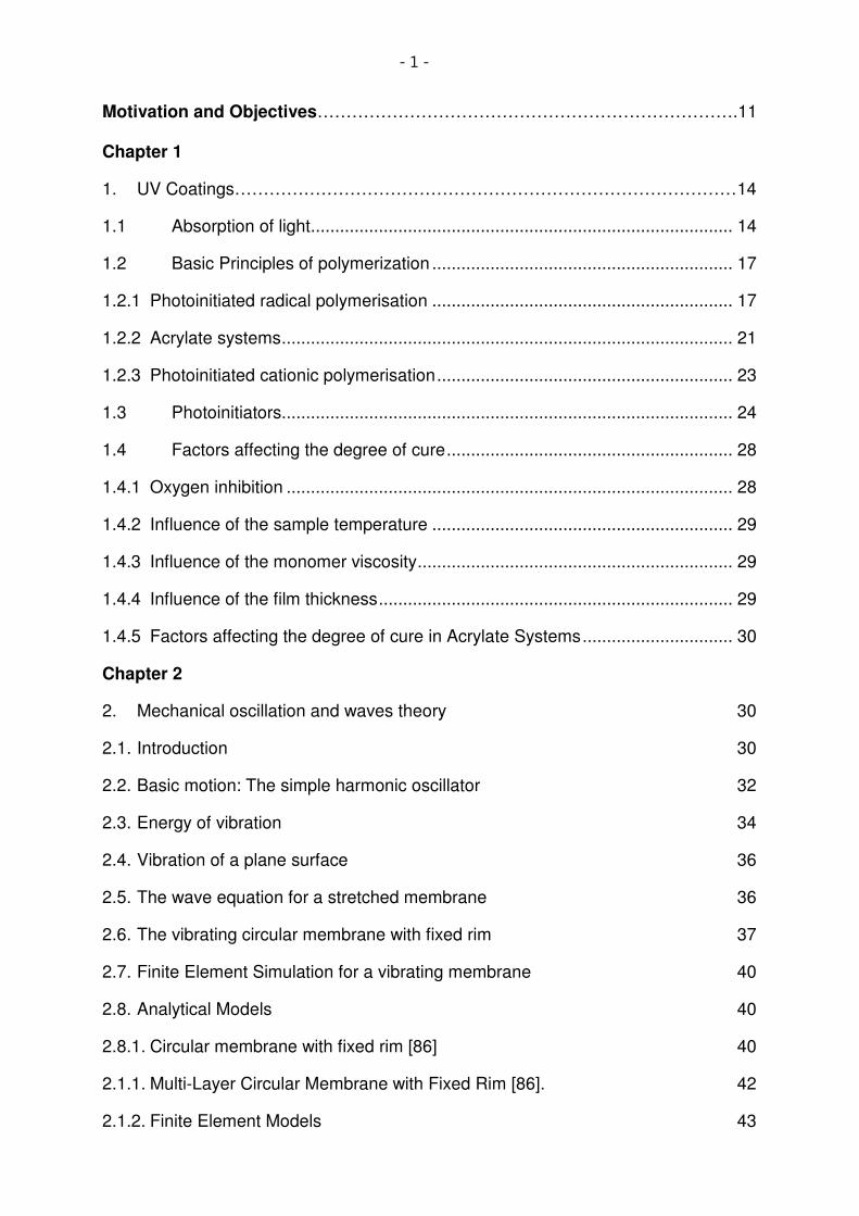
In the the photoinitator system is the benzophenone, which has a long triplet lifetime

(~10-3s) that can be reduced by hydrogen or electron abstraction from substrates or

deactivated by energy transfer to oxygen () [68].

Fig.1. 15: The benzophenon triplet is deactivated by energy transfer to oxygen [68].

In the Type II photoinitiator the synergist plays an important role because of the

competition between them and energy transfer to oxygen. As synergists, most

commonly are employed amines because their high reactivity toward the triplet states

of low energy (40-70 kcal/mol) and their inhibitory effect toward oxygen.

Fig.1. 16: Reaction of triplet benzophenone with an amine synergist.

The photoinitiator used in our formulation were benzophenone and BDK (benzyl

dimethyl ketal) for the clear coating formulation and 2-Benzyl-2-dimethylamino-4-

morpholinobutyrophenon for the pigmented formulation.

- 27 -

Fig.1. 17: The photochemical splitting of BDK (benzil dimethyl ketal) [75].

The BDK (benzyl dimethyl ketal) belongs to the Type I free radical initiators. These

systems derived from benzoin and benzoin ethers and are used to initiate the

polymerisation of acrylate, methacrylate formulations. The BDK represents a very

efficient initiator of this family because of the two alkoxy groups presented in the

benzylic radical. The dimethoxybenzyl radical produced through the splitting

undergoes a thermally activated splitting to formed benzoate.

The choice of photoinitiator depends on a variety of factors, which include how

efficiently they absorb radiation. Considering that the irradiation source is usually a

medium pressure mercury lamp (see Chapter 4), it is fundamental that light of

wavelength 254, 302 and 313 nm is absorbed. In the case of the modified TiO2

nanoparticles is important that light > 380nm is absorbed.

Fig.1. 18: Absorption spectra of benzophenone.

- 28 -

In the case of benzophenone, the absorption is displaced more to the red side and

this effect becomes more pronounced with a benzyl substituent (as in the case of the

pigmented formulation).

Other important factors for the choice of the photoinitiator system are: the film

thickness, the pigment, the type of monomer reemployed in the formulation.

1.4 Factors affecting the degree of cure

1.4.1 Oxygen inhibition

Considering that the UV-curing of acrylate coatings is generally carried out in the

presence of air, oxygen inhibition has always been a key issue [5].

The O2 molecules in the air scavenged the free radicals generates by the

photoinitaitor forming peroxyl radicals.

These radicals do not reacts with the acrylate double bonds but abstract hydrogen

atoms from the polymer backbone creating hydroperoxides (Scheme1).

This process leads to a premature termination reaction and modify the physical and

chemical features of the future polymer.

This can be overwhelming by increasing the photoinitiators amount in the formulation

and increasing the intensity doses of the UV irradiation.

Giving start to a premature termination reaction the oxygen inhibition reduces the

kinetic chain length interpenetrating oxygenated species into the coating.

O2 molecules to yield peroxyl radicals rapidly scavenged the free radicals formed by

the photolysis of the initiator [2, 8]. These species are not reactive towards the

acrylate double bounds and can therefore not initiate or participate in any

polymerization reaction. They usually abstract hydrogen atoms from the polymer

backbone to generate hydroperoxides (Scheme 1).

Moreover, this premature chain termination modifies the mechanical properties of the

film. An additional amount of photoinitiator (and of UV energy) is therefore needed to

consume the oxygen dissolved in the resin, as well as the atmospheric O2 diffusing

into the sample during the UV exposure, in order to obtain tack-free coatings showing

the required mechanical properties.

Oxygen inhibition not only reduces the rate of cure but also affects the properties of

the coating by reducing kinetic chain length (and hence molecular weight) and by

introducing oxygenated species into the coating.

- 29 -

Fig.1. 19: Oxygen reacts with hydrogen atoms from the polymer chain forming hydroperoxides.

The oxygen atoms scavenges the free radical generates by the photoinitiator and

scavenge the chain formation.

This features are enhanced by an increase of the O2 concentration in the

atmosphere, an increase in the sample temperature, a decrease of the viscosity of

the formulation or a thin film where the diffusion of oxygen atoms are facilitated

1.4.2 Influence of the sample temperature

UV curable coatings have usually a high viscosity ranged from 200 to 4000 mPa/s.

The viscosity is decreasing with the temperature, thus allowing a faster diffusion of

the oxygen into the sample. This will reduce the molecular viscosity and therefore will

slow the conversion rate.

1.4.3 Influence of the monomer viscosity

The viscosity of the UV-curable formulation is another factor, which will determine the

rate at which O2 diffuses into the sample. The inhibitory effect of oxygen on the

photopolymerization process is therefore directly dependent on the type of monomer

used as reactive diluents to adjust the formulation viscosity. It will act at two levels:

• The monomer reactivity, which governs the cure speed and therefore the

reaction time during which atmospheric oxygen penetrates into the sample [5,

6].

• The monomer viscosity, which determines the speed at which air diffuses into

the sample. Even if the monomer reactivity is very high, no polymerization will

occur if the oxygen diffusion through the fluid film is very fast.

1.4.4 Influence of the film thickness

Some authors [78] shows that the inhibitory effect of oxygen is more pronounced in

the top layer of the film in contact with air.

Therefore, thin films are more sensitive to oxygen inhibition than thicker ones.

- 30 -

Curing under inert atmosphere has therefore more impact as well as better results for

thin films.

1.4.5 Factors affecting the degree of cure in Acrylate Systems

The UV induced polymerisation is known as an ultra fast process, which transforms a liquid into a solid. The UV induced transitions leads to increase the mixture viscosity to gel state, which on turn will vitrify by further radiation. The photopolymerization of acrylates has as result a linear polymer and usually the new product is a soft solid. Under intense irradiation, the system will register an increase in the viscosity, but in the meantime remains sufficiently fluid to allow a high percentage conversion of the acrylate double bonds. When the polymerization reaction is started by a benzoyl radical, secondary cross linking reactions may also occur, which means that monoacrylates can form crosslinked coatings. The monomer employed in our coatings formulation was a diacrylate, which leads to a pronounced crosslinking. Thus, the onset of gelation and vitrification occurs much early as in the monoacrylates case. Therefore, the early occurrence of the vitrification point may “freeze” some double bonds and the cured coating will contain unreacted acrylate groups. Sometimes these unreacted groups are consumed by prolonged irradiation of the coating through radical transfer in the coating. A very interesting modelling study based on the percolation theory [7] shows that the growth of the polymer occurs in discrete areas rather than the polymer grows throughout the matrix. The development of discrete polymerisation ares can lead to areas of unreacted material and to phase separation. Other specific problem of daicrylates is that the pendant groups produced cyclic structure, which reduced the crosslinking formation. These characteristic togher related to the fact that the glass transition temperature

(Tg) of the cured film id dependent of the cure temperature should be considered by

measuring the mechanical performance of the coatings.

2. Mechanical oscillation and waves theory

2.1. Introduction

In this work we use acoustic waves and the correlated vibrations to detect the extent

of the photopolymerisation phenomenon. The generation, transmission and reception

of energy as vibration waves represent the base of the acoustics. First we will briefly

explain how the acoustic wave is generated and transmitted and we will list the

different wave’s types.

In order to understand the complex motion of the membrane with fixed rim

(described in Chapter 4) we will begin with the simplest type, the one-dimensional

sinusoidal vibration.

- 31 -

Acoustic waves

The displacement from normal configuration of internal molecules, in a fluid or solid,

produces an oscillation due to the elastic restoring forces.

The transfer of this oscillation through all the particles of a medium represents a

mechanical wave.

The most common types of mechanical waves are:

transverse, longitudinal and torsional waves.

Fig.2.1 Propagation of a sound wave [87].

Transverse waves are characterized by a perpendicular displacement to the motion

direction of the wave.

Longitudinal waves are characterized by a displacement that is parallel to the wave

direction.

Fig.2.2 Transverse wave on a string; the displacement of the medium is perpendicular to the

direction of propagation of the wave

Torsional waves are characterized by a rotational oscillation of the medium.

- 32 -

Fig.2.3 Longitudinal Wave Propagation (Top) and Transversal Wave Propagation (Bottom)

The most important vibration motion is the simple harmonic oscillation.

This oscillation results quite significant because it is a simple motion but, on the other

hand, the equation of the simple harmonic oscillation describes also the motion of

other vibration phenomenon.

2.2. Basic motion: The simple harmonic oscillator

The mechanical movement of a mass attached to a string and oscillating from its

equilibrium position represents a sine or cosine function of time.

This type of sinusoidal vibration is called harmonic oscillation.

A harmonic oscillation has to respect Hooks’ law, it means that the restoring force is

directly proportional to the displacement; this is under the assumption that the mass

is constant and the motion is considered ideal (no losses will attenuate the motion).

According to these conditions, the frequency of the oscillation is independent of

amplitude and the motion is simple harmonic.

- 33 -

Fig.2.4 Schematic representation of a simple oscillator consisting of a mass m, attached to one

end of a spring of spring constant c. The other end of the spring is fixed.

According to Hooks´ law the restoring force F is:

F=-cx 2. 1

where “c” is the spring constant in N/m, x is the displacement in meters (m) of the

mass expressed in kilograms (kg).

The minus sign indicates that the applied force opposites to the displacement.

According to the Newton law we have that:

F=mdt

xd ² 2.2

where dt

xd ² is the mass acceleration.

Substituting in 2.1, the general equation of harmonic oscillation becomes:

0²

=+ xm

c

dt

xd 2. 3

Taking in consideration that both “c” and “m” are positive, we can define:

m

c=²ω

2. 4

By substitution in the equation 2.1 we obtain:

x

F = -cx

- 34 -

dt

xd ²+ 0² =xω 2. 5

The solution of such equation is a sinus or cosines function.

Let us then assume that the solution is:

)sin( ϕω += tAx 2. 6

Where A is the amplitude of the oscillation and φ represents the phase angle.

ω is the natural angular frequency measured in radians per second (rad/s). Since

there are 2π radians in one cycle, the natural frequency f in hertz (Hz) is related to

the natural angular frequency by:

π

ω

2=f

2. 7

From equation 2.7 we can observe that the decreasing of the spring constant or

increasing of the mass will lowers the frequency.

The period T of one complete oscillation is given by:

fT

1= 2. 8

Assuming that at the time t=0 the mass has an initial displacement 0x and an initial

velocity 0v by substitution into 2.6 we obtain

)sin(0 ϕω += tAxx 2. 9

The velocity of the particle is given by:

)cos( ϕωω +== tAdt

dxv 2. 10

Similarly, the acceleration is given by:

xtAadtdv 22 )sin( ωϕωω −=+−==

2. 11

2.3. Energy of vibration

- 35 -

The energy of a mechanical system consists of the potential (Ep) and kinetic energy

(Ek) of the system.

The potential energy is the work spent in deforming the spring by moving the mass

from its static equilibrium position. The force exerted by the mass on the spring is in

the direction of the displacement (Fig.2.4) equals +cx, therefore the potential energy

Ep conserved in the spring will be:

2

02

1cxcxdxE

x

p == ∫ 2. 12

By substitution of x from 2.9 we obtain:

)cos(2

1 2 ϕω += tcAE p 2. 13

The kinetic energy of the mass our system is:

2

2

1mvEk = 2. 14

By substitution of v from we have

)(sin2

1 22 ϕω += tmvEk 2. 15

The total energy of our system becomes:

22

2

1AmEEE kp ω=+= 2. 16

where we assume that

2ωmc = 2. 17 and

1cossin 22 =+ αα 2. 18

As we can see the total energy of the system is a constant and is equal to the

maximum potential energy (when the mass is at its greatest displacement) or to the

maximum of the kinetic energy (when the mass passes through its equilibrium

position).

- 36 -

2.4. Vibration of a plane surface

If we consider transverse vibration of two-dimensional systems, such as drumhead or

the diaphragm the equation of motion will be the two-dimensional generalization of

that for a string.

Generalization to two dimensions requires selecting a coordinate system. Choice of

coordinate system matching the boundary condition (Cartesian coordinates for a

rectangular boundary and polar coordinate for a circular boundary) will greatly

simplify the effort to obtain and interpret the solutions.

2.5. The wave equation for a stretched membrane

Let us consider a membrane that is thin, uniformly stretched in all directions and

vibrates transversely with small displacement amplitudes. If ρs is the surface density

(kg/m²) of the membrane and σ is the membrane tension per unit length (N/m), the

material will be pulled apart with a force σ*dl on opposite sides of a line segment of

length dl.

In Cartesian coordinates the transverse displacement of a point is expressed as a

function u(x, y, t).

The force acting on a displaced surface element of area dS=dxdy is the sum of the

transverse forces acting on the edges parallel to the x and y axes.

The net vertical force arising from the pair of opposing tension σx is σ(∂2u/∂y2)dxdy

and that from the pair of tension σdx is σ(∂2y/∂z2) dxdz. Equating the sum of these

two to the product of the mass ρsdxdz of the element and its acceleration ∂2y/∂t2 gives

2

2

x

u

∂

∂

+2

2

y

u

∂

∂

=2

1

c2

2

t

u

∂

∂

2. 19

sc

ρ

σ=2

2. 20

If ∇ is the Laplacian operator (in this case two-dimensional) the 2. 18 represents the

two-dimensional wave equation.

The form of the Laplacian depends on the choice of the coordinate system. The

Laplacian in two-dimensional Cartesian coordinates, 2∇ = ∂²/∂x² + ∂²/∂y², is

appropriate for rectangular membranes.

For circular membranes, which are our case, polar coordinates (r, θ) are preferable

and the Laplacian can be translated into: 2∇ =∂²/∂r²+1/r ∂/∂r+1/r² ∂²/∂θ²

This gives the equation for circular stretched membrane (see 2.4).

Solutions will have all the properties of the previously studied waves, generalized to

two dimensions.

- 37 -

To calculate normal modes on membranes it is conventional to assume the solutions

have the following form:

y= Ψe

iωt 2. 21

where Ψ is a function only of position. Substitution and identification of k=ω/c yields

the Helmholtz equation:

∆

2 Ψ + k²Ψ = 0 2. 22

The solutions of equation 2. 21 for a membrane with specified shape and boundary

conditions are the normal modes of the problem.

2.6. The vibrating circular membrane with fixed rim

The vibrating membrane problem is simply the two-dimensional version of the vibrating string problems. For a circular membrane we have the boundary condition r=a. The Helmholtz equation in cylindrical coordinates becomes:

011 2

2

2

22

2

=Ψ+∂

Ψ∂+

∂

Ψ∂+

∂

Ψ∂k

rrrr θ 2. 23

Assuming that ),( θrΨ is the product of two terms, each of them a function of only one

spatial variable:

)()( θΘ=Ψ rR 2. 24

Supplementary, θ(Θ ) must be a smooth and continuous function ofθ .

By substitution in 2. 22 we become:

rdr

Rd Θ+Θ

2

2

02

2

2

2=Θ+

Θ+ Rk

d

d

r

R

dr

dR

θ 2. 25

withc

kω

= .

Multiplying the equation by Rr Θ/2 and separating the terms containing r to one side and the terms containing θ to the other side we obtain:

2

222

2

22 1)

1(

θd

drk

dr

dR

rdr

Rd

R

r Θ

Θ−=++

2. 26

The two parts of the equation being function of different variable can be equal only for a constant.

Suppose this constant is 2m , equation 2.26 becomes:

- 38 -

Θ−=Θ 2

2

2

md

d

θ 2. 27

with an harmonic solution:

)cos()( mm γθθ +=Θ 2. 28

Since Θ is a smooth and single-value function, each constant m must be an integer. With m fixed in value, the 2. 26is the Bessel equation.

0)(1

2

22

2

2

=−+++ Rr

mk

dr

dR

rdr

Rd

2. 29

The solution is the Bessel function of order m of the first kind )(krJ m and second

kind )(krmΥ ,

)()()( krBkrAJrR mm Υ+= 2. 30

While 2.30 is the general solution of equation 2. 29,, a membrane that extends across the origin must have finite displacement for r=0. That means 0=B so that:

)()( krAJrR m= 2. 31

For the boundary condition 0)( =aR we will have )(krJ m =0.

If the values of the argument of mJ that cause it to equal zero are determinate by mnj ,

then k assumes discrete values a

jk mn

mn = [22].

+= θθ mrkJAtrY mnmmnmn cos()(),,( mntj

mn eωγ )

2. 32

mnmn jak = 2. 33

and the natural frequencies are:

acjf mnmn π2/= 2. 34

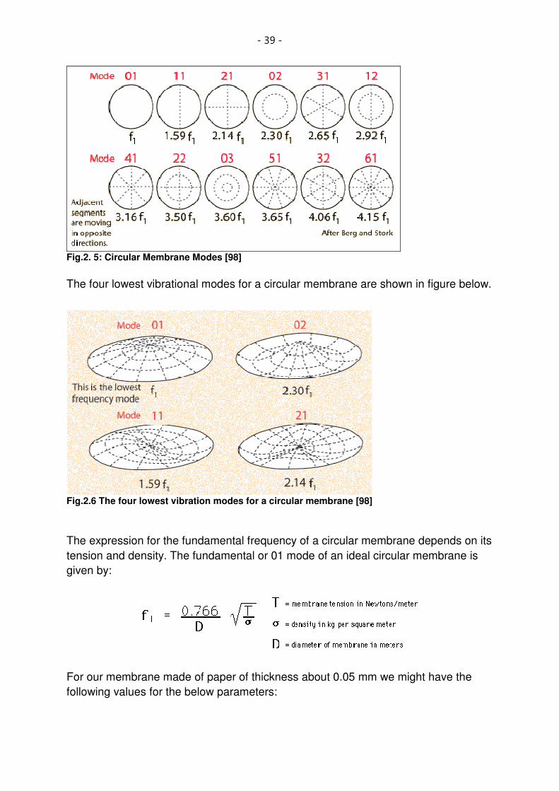
- 39 -

Fig.2. 5: Circular Membrane Modes [98]

The four lowest vibrational modes for a circular membrane are shown in figure below.

Fig.2.6 The four lowest vibration modes for a circular membrane [98]

The expression for the fundamental frequency of a circular membrane depends on its

tension and density. The fundamental or 01 mode of an ideal circular membrane is

given by:

For our membrane made of paper of thickness about 0.05 mm we might have the

following values for the below parameters:

- 40 -

T=753 N/m²

D=0.025m

σ=1 kg/m² f01=350 Hz

T(N/mm²) τ(kg/m³) D(m) f0 f11 f21

753.48 1 0.025 841 1337 1805

The tension has been calculated from an experimentally measured mode (see

Chapter 4).

2.7. Finite Element Simulation for a vibrating membrane

To verify our theoretical model we used a FEM Simulation from Structure Mechanics of Comsol Multiphysics. We began with basic analytical model of simple paper membrane and ended with complex 2-dimensional axis-symmetric finite element model of the paper membrane coated with our acrylate sample. Simulation studies are conducted to illustrate the effect of cure on critical performance parameters such as displacement and eigenfrequency.

2.8. Analytical Models

2.8.1. Circular membrane with fixed rim [86]

The general wave equation for a single layer homogeneous elastic isotropic circular

membrane is:

222

2

2

2 1

t

u

cy

u

x

u

∂

∂=

∂

∂+

∂

∂

2. 35

This is the equation for an ideal membrane (stiffness-free) and ideal plates (tension-

free).

Our membrane made of paper exhibits a Young’s modulus of approximately 365MPa.

The paper average density and thickness were measured at approximately 1kg/m³

and 80 µm respectively.

We assume that damping and inertial forces acts on the surface of our membrane.

Introducing the polar coordinates for a circular membrane and taking into

consideration the stiffness of the membrane, the equation 2. 34 becomes:

D

Q

r

u

r

u

rr

u−=−

∂

∂+

∂

∂22

2 1

2. 36

- 41 -

D

Q

r

w

rr

w

rr

w=

∂

∂−

∂

∂+

∂

∂22

2

3

3 11 2. 37

where φ is the displacement of the membrane, Q is the shearing force, r is the radial

distance from the centre of the circular membrane, w is the displacement of the plate

and D is the flexural rigidify of the plate given by:

)1(12 2

3

ν−=

EhD

2. 38

where E is the Young’s modulus, h is the membrane thickness and ν the Poisson’s

ratio.

When the above circular membrane of a known radius is subjected to a uniform load

intensity q (N/m²), the shearing force Q can be determined from:

2

qrQ =

2. 39

Taking this into consideration equation 2. 35 becomes:

D

qr

r

wr

rrr 2

1=

∂

∂

∂

∂

∂

∂

2. 40

After two integrations, carrying the constants through the results along with the

constants of integration, equation 2. 39 becomes:

r

CrC

D

qr

r

w 21

3

216++=

∂

∂

2. 41

where w is the deflection in the z-axis at any distance r from the centre of the

membrane and C1 and C2 are integration constants that must be evaluated.

Consider now a circular membrane of radius “a” and fixed at the rim. The slope at the

clamped rim and centre of the circular membrane is zero and the boundary

conditions are applied as follows:

0216

0

21

3

=

++

=rr

CrC

D

qr

2. 42

- 42 -

By substitution and simplification, the generic displacement for a single layer circular

membrane fixed at its radial boundaries is:

)(64

22ra

D

qw −=

2. 43

2.1.1. Multi-Layer Circular Membrane with Fixed Rim [86].

For a multi-layer membrane, the behaviour of the system will be different from the

behaviour of a single, homogeneous membrane.

For materials with different Poisson’s ratio a change in the length of the lines will take

place, parallel to the lower material due to an in-plane strain z.

Equation 2. 42 is applicable once “D” is replaced with “De” and a correction factor for

in-plane shear is applied. The equivalent membrane stiffness “De” based on the rule

of mixtures for a two material case can be obtained in the equation below:

p

aa

e KtE

D 22

3

)1(12 ν−= 2. 44

Where,

22

22

22

22

2

)()1(

)1()1)(1(3

)1(

)1(1

bb

aa

ba

bb

aa

bb

aa

a

b

a

aaa

abb

p

tE

tE

tE

tE

tE

tE

t

t

tE

tEK

νν

ν

ν

ν

+−+

++−

+−

−+= 2. 45

where the equivalent Poisson’s ratio is:

p

p

aeK

K

1

2νν = 2. 46

The equivalent Young’s modulus can be extrapolated from the equation of the

equivalent stiffness:

p

bbaa

abab

e KEtEt

EEtwtIE 1

3

)(12 += 2. 47

where “I“ is the Moment of Inertia of the acrylate layer, ta and tb are the thicknesses

of the top and bottom layers respectively; Ea and Eb are the Young’s moduli of the top

and bottom layers respectively and:

- 43 -

)1(

)1(

)1(

)1()(464

3

3

3

3

2

1

baa

abb

abb

baa

b

a

b

a

ptE

tE

tE

tE

t

t

t

tK

ν

ν

ν

ν

−

−+

−

−+++= 2. 48

Taking into consideration this correction for the shear between the materials layers

equation 2. 42 becomes:

−

−+−= )(

1

4)(

64

222

222ra

hra

D

qw

ee ν 2. 49

2.1.2. Finite Element Models

Since the membrane is circular, we were able to take advantage of symmetric

boundary conditions and to model one piece of the overall geometry as shown in

Fig.2.7

Material Young’s

Modulus

Poisson’s

Ratio

Density kg/m³ Thickness mµ

Paper 50 MPa 0.45 1 80

Acrylate 350 MPa 0.55 225 8

Table 2.1: Material data for the paper substrate and the top coating layer.

The above material properties can be assumed to be linear, homogeneous, elastic

and isotropic.

A rectangular slice of the membrane was modelled with symmetric boundary

conditions as shown in Fig.2.7.

We use the Axial Symmetries Stress-Strain application mode in cylindrical

coordinates r, φ and z. It solves the equations for the global displacement u in the r

and z directions [Comsol Multiphysics, Modelling Guide].

The displacement v in the φ direction together with the ϕτ r , τ zϕ and ϕγ r , zϕγ

components of the stresses and strains are assumed to be zero. In this mode loads

are independent of φ and it allows them only in the r and z directions.

The symmetric faces were free in the normal direction to the faces “z” and the circular

ends were clamped in all directions.

The mesh generation was developed in the simulation available COMSOL mesh

generator using Lagrange Quadratic, 2nd order elements (Fig.2.7). The elements

modelled each material layer and identified coincident nodes between materials.

- 44 -

Fig.2.7: Vibrating membrane mesh

2.1.3. Simulation Results

The sample is coated onto membrane as described in the Chapter 4. The thickness

for all acrylate samples lies between 4 and 6µm.

Following the analytical method defined earlier, equation 2. 42 is used to find the

eigenfrequency of the vibrating membrane shown in Fig.2.8 where properties are

given in Table 2.1.

Increasing time cure will increase as well the elastic modulus of the acrylate sample.

Elastic modulus data can be loaded and saved under the setting of our subdomain in

order to be used by the simulator.

The changes in the elastic modulus show a decrease in the eigenfrequency of certain

modes and in the meantime an increase in the certain modes of other modes.

As can be seen from the summary plot the eigenfrequency for the uncured sample

are close in value.

- 45 -

Fig.2.8: Simulation model for a two layer vibrating membrane

We simulated the changes of eigenfrequencies taking in consideration two cases:

- The ideal case, where the paper remains unaltered, respectively the Young

Modulus is fixed at a constant value.

- The real case, where the paper substrate altered under UV light and the

Young Modulus decrease with increasing cure time (see Chapter 5 ).

The plot of the changes, in the ideal case with Young Modulus constant, shows a

small, but constant increase of the eigenfrequencies with increasing of the cure time

and, as consequence, with an increasing photopolymerization.

The simulation results, in the ideal case, are important to evaluate samples printed by

printing machine where the cure time is reduced to a few milliseconds and the

altering of paper substrate is negligible or zero.

The results are to be seen in Table 2.2.

0

500

1000

1500

2000

2500

3000

3500

Eigenfrequencies

(Hz)

0 5 10 20 30 40 50 60

Irradiation time (min)

Increase of the eigenfrequencies with irradiation time

Fig.2.9: Increasing of the eigenfrequencies for a two layer model with increasing cure time (no

alteration of paper occurs)

- 46 -

The real case, checked upon the experimental data, shows a decrease of the

eigenfrequencies with increasing cure time. This data matches the experimentally

obtained data and are to be expected taking in consideration the degradation of the

paper substrate under irradiation (see Chapter 5).

0

500

1000

1500

2000

2500

3000

3500

4000

Eigenfrequencies

(Hz)

0 10 30 60

Irradiation time (min)

Decrease of the eigenfrequencies with irradiation time

Fig.2.10: Decrease of the eigenfrequencies for a two layer model with increasing cure time (paper altering matches’ experimental data)

The experimental data measured for the irradiated paper substrate and for the top

layer coating are listed in the Table 2.2

- 47 -

Young Modulus Substrate (Paper) (MPa)

Young Modulus Top Layer (Coating) (MPa)

Eigenfrequencies (Hz)

Irradiation Time(min)

62.421 345.231 700 1902 3711

0

60.421 346.045 701 1906 3719

5

58.233 346.568 702 1910 3726

10

55.23 346.889 698 1898 3703

20

54.245 347.233 697 1894 3696

30

53.624 347.988 695 1890 3688

40

53.275 348.566 694 1886 3680

50

53.254 348.566 694 1886 3680

60

Table 2.2: Table of the Young Modulus for the paper substrate and top coating layer under

irradiation.

The analytical model matches the experimental data if we take into consideration the

altering of the paper substrate.

In Chapter 6 we will show a parallelism among experimental data and the simulation

results.

- 48 -

3. Standard techniques for investigation of the photopolymerization

3.1. FTIR and Real Time FTIR Spectroscopy

“Nowadays, FTIR spectroscopy is well-accepted as a versatile and powerful

technique for quantitative monitoring in UV-initiated curing processes which proceeds

on a millisecond time scale basis. Due to its high time resolution, curing experiments

can be designed and performed under experimental conditions which are quite close

to those in technical coating and printing processes”[ Klaus-Jochen Eichhorn, D.

Fischer, I. Meisel ] .

For a better understanding of the spectroscopic measurements we will give some

basic information about the molecular vibration and detection.

The system formed of positively charged atomic nuclei surrounded of negatively

charged electrons forms a molecule. The molecule stability depends of the

interactions forces: attractive or repulsive, between the atomic nuclei and electrons.

The energy derived from those interacting forces characterized the molecule and its

allowed energy states are quantized.

The absorption or emission of electromagnetic radiation of a molecule during the

change from one energy state to another is known as molecular spectra. The

molecular spectra are a result of all contributions from different types of molecular

motions and energies.

Basically, two major types of interactions are responsible for the molecular spectra.

The first type consists of the internal motions of the nuclear system of the molecule

and the attractive and repulsive forces among the atomic nuclei and electrons. The

second type refers to the interactions between electrons.

The first type of interactions consists of electronic, vibration and rotational motions.

The electrons in a molecule have kinetic energy resulting to their motion and potential

energy resulting from the attraction to the positively charged nuclei and their

reciprocal repulsion. These two types of energy together with the potential energy

resulting from the reciprocal electrostatic repulsion of the positively charged nuclei,

represents the molecule electronic energy. The interaction of electromagnetic

radiation, commonly monochromatic light, with these molecular energy levels

represents the basis of the almost used spectroscopy: electron, visible, infrared (IR),

Raman, ultraviolet (UV).

The second type of interactions are used in nuclear magnetic resonance (NMR)

spectroscopy and electron spin resonance (ESR) spectroscopy and consists of the

reaction between the nucleus magnetic moment or an electron with an external

magnetic field. The interaction is strongly dependent of the nucleus or electron

molecular environment.

- 49 -

When a molecule undergoes absorption or emission of electromagnetic radiation will

be registered an increase or decrease in energy. The quantum mechanics imposed

that each pair of energy levels can contribute in energy changes and therefore to the

extent of the radiation absorbed or emitted.

A molecule in transition from a lower energy state to a higher energy state absorbs

electromagnetic radiation when:

νhEE lh =− 3. 1

Inversely, a molecule in transition from a higher energy state to a lower energy state

emits electromagnetic radiation with the frequency v. Those phenomenons are

known as induced absorption and induced emission respectively.

3.1.1. Rotational energy states

Considering the diatomic model of a molecule with two atoms of masses 1m and

2m situated at the distance r, the moment of inertia of the molecule will be

2rI µ= 3. 2

where µ represents the reduced mass and is defined as

)( 21

21

mm

mm

+=µ 3. 3

The rotational energy of the system according to the quantum mechanics law

)8/)(1( 22 IhRREr π+= 3. 4

where h is the Planck constant and R=0, 1, 2, represents the rotational quantum

number.

The molecular rotational spectra can be observed by molecules which undergoes

transitions from one rotational level to another according to the allowed changes in

the quantum number which characterized the energy states of the molecule.

Returning to the diatomic model, it means the molecule should have a two different

atoms to guarantee a permanent dipole moment, the frequency of the radiation

incident have to accomplish eq. νhEE lh =−

3. 1 and 1±=∆R . The energy emitted in a transition from the level R to the

level 1+R will be

)8/)(1(2 22

1 IhRhvEE RR π+==−+ 3. 5

)1(2 += RBv 3. 6

- 50 -

IhB28/ π= 3. 7

3.1.2. Vibrational energy states

The quantization of molecular energy levels and the derived absorption or emission

of radiation is complicated with respect to the atoms where responsible for it is the

interaction of the electrons with the nucleus and with other electrons. To understand

those mechanisms the literature used the diatomic model.

The rotational motion occurs in real molecules which are not rigid, but can rotate

around their bonds. Considering the diatomic model, where the two nuclei are in

permanent motion to one another and that the oscillatory motion should respect the

quantum mechanics rules, the vibration energy should follow the Schrödinger

equation:

00 )2/1(2)2/1( hvvxhvE ev +−+= ν 3. 8

where ,...2,1,0=ν represents the vibration quantum number and

ex represents the molecule’s equilibrium position.

In the case of a harmonic vibration motion, the potential energy:

2

2

1kxE p = 3. 9

is the same as for the harmonic oscillator.

The real molecule it is difficult to find a perfectly harmonic motion. For the harmonic

motion, the second term of the equation 3. 8 will predominate, when the anisotropy

constant 1≤eα . In this case the potential energy of the system can be described with

the Morse potential:

2))](exp(1[ eep rrDE −−−= β 3. 10

where the factor eD represents the energy of dissociation and

2/1

0 )2

(2eD

vµ

πβ = 3. 11

Equation 3. 11 contains the reduced mass, µ and the vibration energy in the ground

state, 0ν . Considering this, the bond constant can be define as

µπ 2

0 )( hvk = 3. 12

- 51 -

In the case of a molecule with N atoms the number of chaotically vibration motions

can be reduced because of the symmetries to a limited number of normal

vibrations Z :

TRNZ −−= 3 3. 13

Z corresponds to the molecule degree of freedom and is define of the number of

atoms, N which can independently move in the 3 space directions less the 3

translations degree of freedom, T and the 2 to 3 rotational degree of freedom, R for

the stretching and the angular case respectively. The energetically distance between

the vibration energy state from ν=0 to v=1 is with 200 to 4000 wave numbers in the

zone up to the thermal excitation [10]. The thermal energy is, at 25°C, approximately

207 wave numbers (25meV ~207cm). The lower energy state is the most populate by

vibration motion and for the harmonic motion only transitions 1±=∆v are allowed.

This considerations makes that the transitions starting or ending at the lower energy

level have more probability to be detected.

3.1.3. Optical transition and IR absorption

The molecular spectra can be observed when a molecule interacts with an

electromagnetic radiation. The molecule should exhibit a dipole moment that changes

along the normal coordinate and interacts with the oscillating electromagnetic field.

According to the quantum mechanics rules, a radiation induced transition is allowed

when the transition probability 0|| ≠nmR . Because the transition probability depends of

the dipole moment we will have:

|| nmR =2*2*2* )()()( mznmynmxn ΨΨ+ΨΨ+ΨΨ µµµ 3. 14

When nΨ is orthogonally to mΨ the vibration motion will be harmonic and leads to the

selection rule 1±=∆v [11].

In the following paragraph we will illustrate a few notion and concepts that are

indispensable for the spectroscopy measurements comprehension.

3.1.4. The Lambert-Beer law

In all spectroscopy measurements it is important to known how much from the

radiation transmitted to a sample will be absorbed from the material. Beer and

Lambert [12] were the first scientists that correlated the transmission of the light

through a sample, the absorption of the sample material and the distance the light

travels through the material (the path length).

ODdcI

IE R =⋅⋅== λε)log( 3. 15

- 52 -

They affirm that the extinction E, optical density OD, is proportional to the

concentration of the sample, the radiated film thickness d and from the wave

dependent, extinction coefficient λε . The law in this form is valid only for samples

diluted in solution by ideal reflex ion measurements. In the molecular absorption

spectroscopy is used the derivation of the form where the extinction is related to the

wavelength.

rI

IT = 3. 16

where T represents the transmission, I the incident and Ir the emitted beam respectively. The equation is the form used to define the intensity absorption in the infrared spectroscopy. When we compare the relative transmission or extinction of different samples can be useful to define those terms through the absorption:

A=1-T 3. 17

In the case of the samples measured on the ATR prism this was complicated

because we had a homogenous film and therefore quantitative analysis was difficult.

The conversion of the transmission data )(λaT allowed limited analysis different

measurements. The value of the reference band )(aTa corresponds to the initial

(before conversion) transmission value and )(aTR corresponds to the value of the

reference band after conversion.

−

−

−−= ))(1(

)(1

)(11))(( aT

aT

TTT R

a

a

an

λλ 3. 18

3.1.5. Snell’s law

The refraction and reflex ion represents along with the absorption and scattering the

most important effects by sample’s irradiation. In we can see the transition of a light

beam from the media with the refractive index n1 to the media with the refractive

index n2. In the case of isotropic media refraction and reflexion can be explain

through the classical optic laws.

- 53 -

Fig.3. 1: Refraction of light at the interface of two media of different refractive indices. [92]

The incident angle aθ is the same as the outfall angle aθ (). The Snell’s law is valid by

transition from an optical dense media to an optical thin media. The ratio of the sinus

of the angles of incidence and of refraction is inversely proportional to the ratio of the

media index and therefore proportional to the ratio of the velocity of light in the two

media.

2

1

1

2

sin

sin

c

c

n

n

b

a ==θ

θ 3. 19

The refraction succeeded by the ATR technique when the light beam changes from

the crystal optical dense media to the optical thin media of the sample.

3.1.6. Fresnel equation

The Snell’s law determinates the direction of the refracted beam but information’s about the fraction of the transmitted and respectively reflected beam we obtain from the Fresnel equation. The equation named after it’s discover offers the possibility to calculate the fraction of incident light beam reflected by the interface between two media of different refractive index:

2

21

21

0 )cos()cos(

)cos()cos(

+

−=

ba

baref

nn

nn

I

I

θθ

θθ 3. 20

Considering that the sum of the intensities of the reflected and the refracted beam is

one, the refracted fraction can be also determinate. When the light beam moves from

a media with the refractive index n1 to the second media with the refractive media n2,

- 54 -

the incident beam undergoes two transitions. In the particular case of the incident

angle greater as the critical angle all light will be reflected therefore the transmitted

fraction will be zero and the reflected fraction one. The critical angle, also known as

the Brewster’s angle represents the particular angle where, for a given n1 and n2, the

value of Rp goes to zero and a p-polarised incident ray is totally reflected.

3.2. FTIR measurements

We have used two different techniques for investigated our samples:

- Real Time FTIR to measure in-situ the degree of conversion on the monomer

- FTIR Spectroscopy for routine monitoring of the samples vibration bands.

Photopolymerization kinetic profiles during UV-induced free-radical polymerizations

were recorded using real-time FTIR (RTIR) in attenuated total reflection (ATR).

This technique permits the thin sample layer to be studied horizontally, i.e. in the

orientation direction which is used in most technical UV curing plants. Moreover, it

simplifies sample handling and the geometry of the irradiation. In the present study, a

horizontal diamond ATR unit is used for sampling. Such a device has some further

fundamental advantages for the investigation of photopolymerization reaction. Due to

the small surface area of the crystal (2x2mm), it can be homogeneously irradiated.

After curing, the crosslinked sample can be easily detached from the diamond simply

by scratching it away.

3.2.1. Experimental Data

Infrared spectra were recorded in real time with Digilab FTS 6000 FTIR Spectrometer

and a Nicolet Model 760 Magna Series II, respectively.

The spectrometer is equipped with a MCT detector and achieves a maximum

temporal resolution of 11ms at a spectral resolution of 16cm-1.

Samples were studied with the ATR technique using a single reflection diamond unit

(“Golden Gate”, Graseby Specac) which is heatable up to 200C (Fig.3. 2).

UV irradiation was performed with an Osram HBO 103 W mercury arc lamp equipped

with a water filter for blocking infrared radiation.

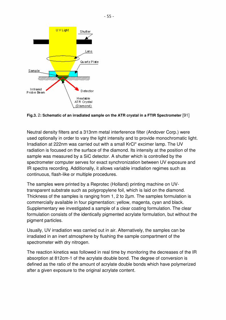
- 55 -

Fig.3. 2: Schematic of an irradiated sample on the ATR crystal in a FTIR Spectrometer [91]

Neutral density filters and a 313nm metal interference filter (Andover Corp.) were

used optionally in order to vary the light intensity and to provide monochromatic light.

Irradiation at 222nm was carried out with a small KrCl* excimer lamp. The UV

radiation is focused on the surface of the diamond. Its intensity at the position of the

sample was measured by a SiC detector. A shutter which is controlled by the

spectrometer computer serves for exact synchronization between UV exposure and

IR spectra recording. Additionally, it allows variable irradiation regimes such as

continuous, flash-like or multiple procedures.

The samples were printed by a Reprotec (Holland) printing machine on UV-

transparent substrate such as polypropylene foil, which is laid on the diamond.

Thickness of the samples is ranging from 1, 2 to 2µm. The samples formulation is

commercially available in four pigmentation: yellow, magenta, cyan and black.

Supplementary we investigated a sample of a clear coating formulation. The clear

formulation consists of the identically pigmented acrylate formulation, but without the

pigment particles.

Usually, UV irradiation was carried out in air. Alternatively, the samples can be

irradiated in an inert atmosphere by flushing the sample compartment of the

spectrometer with dry nitrogen.

The reaction kinetics was followed in real time by monitoring the decreases of the IR

absorption at 812cm-1 of the acrylate double bond. The degree of conversion is

defined as the ratio of the amount of acrylate double bonds which have polymerized

after a given exposure to the original acrylate content.

- 56 -

Fig.3. 3: Concentration of the double bond of an acrylate sample

In order to overcome the disadvantage of the transparent substrate and to monitor

the decrease in the acrylate double bond, at 812 and 816 respectively, we routinely

take the IR spectra of un- and irradiated samples (see Fig.3. 4)

Fig.3. 4: The decrease in the double bond band (CH=CH2) of the functional group

indicates the degree of polymerization.

The degree of conversion (x) is directly related to the decrease of the IR absorbance

[13, 14], and was calculated from the equation:

100(%)0

0 xA

AAx t−

= (3. 21)

- 57 -

where x (%) represented the degree of conversion, A0 and At represent the area of

the IR band centered at 810 cm−1, before and after UV exposure during time t. From

the conversion versus time curves recorded by real time infrared (RTIR)

spectroscopy, we can evaluate the maximum rate of polymerization (Rp)max, by

multiplying the maximum slope (dx/dt)max (also called reactivity) with the initial

concentration in acrylate double [M]0:

0maxmax ][)()( Mdt

dxRp = (3. 22)

The acrylate conversion of the surface layer was evaluated by attenuated total

reflectance (ATR) infrared spectroscopy by using a germanium crystal and

measuring the decrease of the IR band at 810 cm−1 of the UV-cured coating. In both

cases, the induction time is on the order of 0.1s, the time needed for the initiating

radicals to consume the stabilizer and to reach their steady state concentration. Once

started, the polymerization proceeds rapidly, with a reactivity (Rp/ [M] 0)max value of 3

s−1. The reaction starts to slow down only above 50% conversion, once molecular

mobility restrictions brought upon by the viscosity increase and progressive gelation

of the sample become important. In the presence of air, the polymerization starts

after an induction period of 0.2 s, at a speed four times lower as in an inert

atmosphere (Fig. 3.2). After 0.35 s, once 15% of the acrylate double bonds have

polymerized, the reaction begins to slow down because of the continuous diffusion of

air into the sample. (Fig.3.5)

Fig.3.5: Polymerization profiles recorded by RTIR spectroscopy for a sample exposed to UV

light under different atmospheres.

The FTIR and FTIR in real time measurements are the most used method of

quantification of the photopolymerization reaction. In the case of the multifunctional

acrylate coatings, during the photopolymerization process the acrylate double bond is

converted in an aliphatic chain. The rate of conversion can be measured by FTIR

spectroscopy. The functional group in the coating exhibits a specific peak in the IR

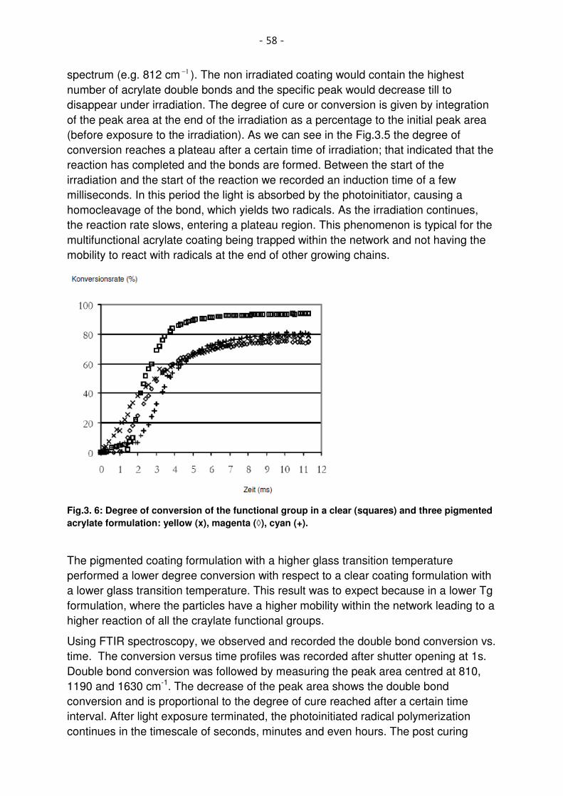
- 58 -

spectrum (e.g. 812 cm 1− ). The non irradiated coating would contain the highest

number of acrylate double bonds and the specific peak would decrease till to

disappear under irradiation. The degree of cure or conversion is given by integration

of the peak area at the end of the irradiation as a percentage to the initial peak area

(before exposure to the irradiation). As we can see in the Fig.3.5 the degree of

conversion reaches a plateau after a certain time of irradiation; that indicated that the

reaction has completed and the bonds are formed. Between the start of the

irradiation and the start of the reaction we recorded an induction time of a few

milliseconds. In this period the light is absorbed by the photoinitiator, causing a

homocleavage of the bond, which yields two radicals. As the irradiation continues,

the reaction rate slows, entering a plateau region. This phenomenon is typical for the

multifunctional acrylate coating being trapped within the network and not having the

mobility to react with radicals at the end of other growing chains.

Fig.3. 6: Degree of conversion of the functional group in a clear (squares) and three pigmented

acrylate formulation: yellow (x), magenta (◊), cyan (+).

The pigmented coating formulation with a higher glass transition temperature

performed a lower degree conversion with respect to a clear coating formulation with

a lower glass transition temperature. This result was to expect because in a lower Tg

formulation, where the particles have a higher mobility within the network leading to a

higher reaction of all the craylate functional groups.

Using FTIR spectroscopy, we observed and recorded the double bond conversion vs.

time. The conversion versus time profiles was recorded after shutter opening at 1s.

Double bond conversion was followed by measuring the peak area centred at 810,

1190 and 1630 cm-1. The decrease of the peak area shows the double bond

conversion and is proportional to the degree of cure reached after a certain time

interval. After light exposure terminated, the photoinitiated radical polymerization

continues in the timescale of seconds, minutes and even hours. The post curing

- 59 -

process can be better examinated using ESR (Electron Spin Resonance)

spectroscopy.

3.3. Differential Scanning Calorimetry (DSC)

During cure, also the viscoelastic properties of the sample change considerably with

increasing conversion at a given curing temperature.

Differential Scanning Calorimetry is a thermoanalytical technique in which the

difference in the amount of heat required to increase the temperature of a sample

and reference are measured as a function of temperature. Both the sample and

reference are maintained nearly at the same temperature throughout the experiment.

Generally, the temperature program for a DSC analysis is designed such that the

sample holder temperature increases linearly as a function of time. The reference

sample should have a well-defined heat capacity over the range of temperatures to

be scanned.

Differential Scanning Calorimetry (DSC) is considered an effective method of

obtaining comprehensive qualitative, and as well quantitative, information on the

curing of UV cured coatings. DSC analyses of the cure kinetics of epoxy resins have

been discussed in a number of studies [15] and various models are available to

quantify the kinetics of reactions as a function of time and temperature.

Reaction kinetics were measured by isothermal curing experiments under nitrogen

atmosphere performed at various cure temperatures, Tcure , using a photo-differential

scanning calorimeter (Perkin-Elmer)

Fig.3.7: Schema of a DSC (differential scanning calorimeter) [92]

- 60 -

Fig.3.8: Typically isothermal curve of a sample obtained with DSC analysis

The Photo-Differential Scanning Calorimetry (Photo-DSC) is a good technique to

investigate the polymerization kinetics and the conversion of double bonds as a

function of exposure time and can be used as reference method. Samples were

weighed into an aluminum DSC pan, purged with N2 and irradiated with filtered UV-

light (320-500nm) from a light guide (8.8mW/cm² at the surface of the sample).

From the heat flow versus time curve characteristic values such as the rate of

polymerization (Rp) can be calculated. Assuming that the heat evolved is proportional

to the number of monomer moles reacted, the degree of monomer conversion (α) as

a function of time can be calculated from the following equation:

%)(100)/(100)]/[][]([ 00 molxHHxMMM ttt =−=α 3. 23

0][M and tM ][ represents the monomer concentrations before and after time (t)

irradiation. H0 is the heat of polymerisation associated with total conversion of

monomer and Ht is the heat liberated after irradiation for time t. To have a solution for

such equation it is necessary to know the amount of heat liberated upon full

conversion. This may be calculated or alternatively determinate experimentally.

Therefore if a simple monoacrylate sample is photopolymerised, with the heat

liberated being determined and the degree of conversion of monomer measured by

i.r. spectroscopy the amount of heat liberated for conversion of an acrylate bond can

be calculated. A typical heat output with time is shown in Fig.3.9 by the clear coating.

The total amount of heat evolved in the reaction is given by the area under the curve.

- 61 -

Fig.3.9: In-situ measurement of a clear and pigmented coating. The clear coating exhibits the

higher degree of conversion; the second one is the yellow pigmented coating, follows by the

black and blue pigmented coating.

Methode: 25-5-min-UV-250

25,0°C 5,0 min N2, 10,0 ml/min

25,0°C 5,0 min UV-Quelle, 10,0 ml/min

25,0°C 5,0 min N2, 10,0 ml/min

25,0-250,0°C 5,00°C/min N2, 10,0 ml/min

250,0°C 5,0 min N2, 10,0 ml/min

250,0-25,0°C -10,00°C/min N2, 10,0 ml/min

Integral 350,02 mJ

blau, 20.06.2007 17:11:01

blau, 15,6860 mg

schwarz, 21.06.2007 09:08:52

schwarz, 25,4260 mg

gelb, 21.06.2007 10:57:57

gelb, 16,2990 mg

ohne-Pigment, 21.06.2007 15:20:01

ohne-Pigment, 8,5480 mg

mW

5

min

°C25,0 25,0

5,0 5,5 6,0 6,5 7,0 7,5 8,0 8,5 9,0 9,5

- 62 -

Fig.3.10: Thermogram of a clear coating (black) and pigmented coatings. The clear coating

reaches the higher degree of conversion; meanwhile the black pigmented coating exhibits the

lower degree of conversion.

The DSC is a useful instrument to determine the different states and transitions in

polymers and soft matter. The DSC measurements can assign the static glass

transition temperature (Tg) and can help to identify the phase transitions of specific

amorphous regions. The identification of glass transition temperature point and the

specific phase transitions in our samples are helpful for the interpretation of the

behavior during the photopolymerization process of our samples.

The photo-DSC, in particularly, was developed for the necessity of a better

understanding and investigation of the polymerization in polymers (thermosets,

curable coatings and adhesives, curable plastics).

The investigated samples showed different rate of photopolymerization. The clear

coating sample reached the glass transition temperature in less 4 than 50 seconds

under 5minutes UV irradiation at T=25°C. The pigmented samples showed a very

slow reaction at T=25°C, therefore we heated the oven with 5°C/min up to 80°C.

The clear sample show an endothermic reaction induced through the temperature

increase. The yellow, magenta and cyan pigmented samples developed the

polymerization reaction at slow rate, meanwhile the black pigmented exhibits only

minimal reaction signs.

Assuming that we can deduce that the pigment added to the formulation of coatings

plays an inhibitor role in the photopolymerization reaction. The energy absorption

Methode: 80°C-UV-5-min-250

25,0-80,0°C 10,00°C/min

80,0°C 5,0 min N2, 10,0 ml/min

80,0°C 5,0 min UV-Quelle, 10,0 ml/min

80,0°C 5,0 min N2, 10,0 ml/min

80,0-250,0°C 5,00°C/min N2, 10,0 ml/min

250,0°C 5,0 min N2, 10,0 ml/min

250,0-25,0°C -10,00°C/min

Integral 33,88 mJ

normalis. 3,00 Jg -1

Integral 6,24 mJ

normalis. 0,87 Jg -1

Integral 55,54 mJ

normalis. 6,99 Jg^-1

Integral 709,00 mJ

normalis. 89,74 Jg^-1

Gelb-80°C-250, 22.06.2007 10:13:09

Gelb-80°C-250, 7,9470 mg

Rot-80°C-250, 22.06.2007 14:03:34

Rot-80°C-250, 7,1620 mg

Blau-80°C-250, 25.06.2007 10:16:19

Blau-80°C-250, 11,2940 mg

schwarz-80°C-250, 25.06.2007 12:42:38

schwarz-80°C-250, 12,2340 mg

Klar-80°C-250, 25.06.2007 14:59:52

Klar-80°C-250, 7,9010 mg

mW

10

min

°C80,0 80,0

10,5 11,0 11,5 12,0 12,5 13,0 13,5 14,0 14,5 15,0

- 63 -

follows by the clear coating formulation according to the Lambert-Beer law (see eq.

3.3); meanwhile by the pigmented coatings (particle mµ1≤ ) we have to consider the

scattering effects.

The extinction E λ (the absorbance of the coating for a light of wavelength λ ) is given

by,

lcI

IE λλ α=−= )lg(

0

3. 24

where,

• I: Intensity of the UV- light

• I0: Intensity of the incident UV light

• c: concentration of the absorbing substance in the liquid sample film (mol/m³

or mol/L)

• αλ: molar extinction coefficient at λ .

• l: optical path length of the light in the given film (cm).

The pigment particles in the pigmented coatings absorb the UV light according of the

Mie scattering theory. The Mie theory consists in an analytical solution of the

Maxwell’s equation for the scattering of electromagnetic radiation by spherical

particles (also called Mie scattering). This solution regards the particles whose size

is similar to the wavelength and offers an analytical approach for the situations

where, the Rayleigh scattering model for small particles or the Rayleigh-Gans-Debye

model for large particles breaks down. The Mie approach is the calculation of the

electric and magnetic fields inside and outside a spherical object and is generally

used to calculate either how how much light is scattered, the total optical cross

section, or where it goes, the form factor. The notable features of these results are

the Mie resonances, sizes that scatter particularly strongly or weakly [16].

We can conclude that a short wavelength realize a higher polymerization rate and

therefore a higher degree of polymerization, in particulary for the pigmented thin film

coatings, where the oxygen inhibition effect is noteworthy (Chapter 1).

For the in-situ measurements, the investigated, unpigmented clear coating acrylate

sample exhibits the higher degree of conversion. The rate of crosslinking was clearly

higher as the rate of crosslinking in the pigmented samples.

In conclusion we want to mention some limitations of this method. The time constant

(response time) of the instrument may be such that for fast reactions the heat output

versus time graph may be distorted. Another difficulty is associated with the samples

pans used with the equipment. It is very difficult to obtain a uniform depth of sample

due to the liquids creeping up the walls of the container. So it can happen to obtain a

sample with a thickness much greater than that of the coating for which the

formulation is to be used. That will affect the cure and the results. Nevertheless the

method is of real value for as labor technique.

- 64 -

3.4. Electron paramagnetic resonance (EPR)

Electron paramagnetic resonance (EPR) or electron spin resonance (ESR)

spectroscopy is an established technique for detection of chemical species with

unpaired electrons. The excitation principle of the EPR spectroscopy is similar to

those of the NMR spectroscopy. Considering that by both techniques the

protagonists are the unpaired electrons the EPR spectroscopy can be applied to

determinate the electronically and geometrical structure of different bonds as well as

the dynamic, concentration and life cycle of radicals. Commonly the ESR

spectroscopy is used to identify paramagnetic species, whereby one can see the

limits of this technique, because only radicals can been identify and those have a

sufficiently long life cycle. ESR spectroscopy is a non destructive measurement

technique; it means the samples rest intact during and after the measurement. The

detection limit of the ESR spectroscopy is .10 9M

− assuming this a time resolution

from 100 to 10 ns is available. Our interest was in the detection of free radicals in our

coatings as well as in the signal dynamic. The literature [Weil et al., Justice] offers

enough studies about the most important interactions (see Fig.3. 11). As can be seen

all transitions need very little energy equivalent to the thermal energy at the room

temperature.

- 65 -

Fig.3. 11: Overview of the principle interactions and their range in the EPR spectroscopy. [89]

Unpaired electrons exhibit an own magnetic field also called spin. Considering Dirac quantum mechanics the unpaired electrons positioned in a static magnetic field can take two possible orientation of the spin (Fig.3. 12): the “parallel” state corresponding to the magnetic field orientation and the “antiparallel” state (Zeemann splitting) corresponding to the splitting of the displacement of the energy levels in a multiple spectral lines.

The measurement principle based on the splitting of the energy level of each electron

in the presence of a magnetic field. The splitting is directly proportional to the

magnetic field’s strength (see diagram below).

Consider the magnetic moment for an electron,

µ s = )1( +ss · µB · g s

(s = Spin quant number = 1/2, µB = Bohr magneton, g s = 2.0023 Lande` -factor for

the free electron).

The ESR spectroscopy based on the absorption of microwave radiation through unpaired electrons, located in a static magnetic field.

- 66 -

Fig.3. 12: Orientation of unpaired electrons in a static magnetic field. [89]

If the electron is positioned in a static magnetic field, the component along the z axis will be,

(µ s ) Z = ± 1/2 µ B · g s with the energy

E = ±1/2 g s · µ B · B and the energy difference ∆ E = g s · µ B · B.

∆ E = h · υ = g B · µ B · H 0 3. 25

h = Planck constant = 6,6260755 · 10 34− J s

υ= microwave frequency [s 1− ]

g = Landé-factor (g-value)

H 0 = [T = Tesla]

µ B = Bohr magneton = 0,92740154 · 10 23− J T 1−

Fig.3. 13: Energy splitting of an electron in presence of a magnetic field [93]

- 67 -

Usually the EPR spectra can be obtained by modifying the photon frequency on the

sample by constant magnetic field or vice versa.

The measurements can be performed in two modes: varying the microwave

frequency at constant magnetic field or varying the magnetic field at constant

microwave frequency.

For technical reasons the second variant is the most used.

The schema of the resonator with the microwave bridge can be seen in Fig.3. 14.

Fig.3. 14: Schematic of the ESR resonator. [89]

The radiation source, a Gunn diode, generates a microwave in the range from 9-10

GHz (X-band). This corresponds by a g-value of 2, 0023 to a magnetic field of 323, 9-

359, 9 mT (1mT=10Gauss). The microwave frequency is constant during the

measurement period and it is forwarded, through a waveguide or a coaxial cable, into

the sample holder. The sample holder is constitutes of cavity with rectangular or

cylindrical form. In the cavity will be generate through the right coupling (tuning) a

standing wave. Because the changes in the amplitude of this wave, by a linear scan

of the magnetic field are to small to obtain an appropriate signal to noise ratio, the

magnetic field it is modulated, during the measurement, from a low to a higher field

(scan) with supplementary 100 kHz. The amplitude of the oscillation of the magnetic

field can be varying in the range of 10 µT-1mT (X-band). The modulation of the

magnetic field strength is the reason why the ESR spectrum corresponds to the first

derivative of the absorption spectrum of the microwave radiation as function of the

magnetic field strength.

- 68 -

Fig.3. 15: The differential scan of the absorption spectrum gives, because of the modulation of the magnetic field strength, the original ESR spectrum (I-derivative of the absorption spectrum). A: absorption spectrum of the microwave radiation; B: Original ESR spectrum. [89]

The resonance condition for a sample is complied, when the energy ∆ E between the excitated and the single state, corresponds with the energy of the constant microwave frequency for a given magnetic field strength (Fig.3. 19).

Fig.3. 16: The resonance condition by energy splitting. [89]

When the resonance condition is accomplished, the system will absorb the microwave radiation.

The ESR spectrum represents the intensity (∆I), the changes in the microwave amplitude between the modulated magnetic field maximum and the minimum of the

- 69 -

magnetic field strength, divided by the modulation amplitude (∆H) of the magnetic field as a function of the magnetic field strength.

3.5. Magnetic resonance and chemical bonds

The ge factor becomes a material specific tensor when the electron of a molecule is bonded to its atom. The absorption takes place at the resonance with the excitation

or Lamor frequency, Lv :

0Bghv BL µ= 3. 26

In the case of carbon radicals the value of the g factor is practical identical with the

Lande´ factor, because the change in the angular moment of the electron is

insignificant. The hyperfine coupling α with the nuclear spin 0≠I is very important for

the detection and identification of the radicals, because it can leads to a change in

the local magnetic field locB :

lloc maBB ⋅+= 3. 27

The magnetic quantum number lm can assume only the values

.,1,...,1, IIIIml −+−−= 3. 28

In the isotropic cases not all transitions of the combination between electron spin and

nuclear spin are allowed , but only those where the nuclear spin state rest

unchanged .0=∆ Im Assuming N represents the nuclei number adjacent to the orbital

where moves the free electron, we can calculate the number ne of the allowed

transitions:

)12( +⋅= ∏N

K

Ke In 3. 29

This splitting behaviour is similar to those in the NMR spectroscopy. The transitions

number can be reduced through convenient setting of the measurements conditions.

For example, three protons adjacent to a methyl group at the room temperature can

be considered as a one nucleus. The lines intensities resulting from the transitions

number by the same energy corresponds mathematically to the distribution of an

emnucleisystI K 2/1= and will follow the Pascal’s triangle.

3.6. Detection and interpretation of an ESR signal

In the ESR spectroscopy, similarly to the NMR spectroscopy direct absorption measurements are not possible. The reason is that the energy difference between the two spin states is smaller as the thermal energy. The ESR spectroscopy detects the radical’s population for the spin in the ground and excited state. As already mentioned it is use to work with a cavities of sizes in the same order as the

- 70 -

wavelength of the magnetic field. Typical sizes for the X-Band spectrometer are λ=3, 15 cm and cavity size λ/2xbxλ. A standing wave will be generated and by exactly fitting or critical coupling leads, in absence of electrical impedance, to an unendless elevation of the field. This set-up is sensitive to the fines changes in the microwave energy. The quality factor Q of the cavity can be calculated from the electrical impedance and represents the sensitivity of the apparatus and technique respectively:

R

LQ

ω= 3. 30

When the sample positioned into the cavity will be irradiated with a microwave of a

certain wavelength, the spin system of the sample will be excitated. The return of the

spin system to its balance population is defined as longitudinal or spin-lattice

relaxation T1. The second vibration is the transversal T2 also called coherence or

spin-spin relaxation. The second relaxation corresponds to the time when the spins

phase relation ended. This time has impact on the detection because the there are

no x-, y- components of magnetization, Mx, My. This process follows without energy

change. A spin transited from +1/2 to -1/2 and other spin transited from -1/2 to +1/2.

The literature [17] gives a method to calculate the magnetisation for a spectrometer

by known cavity size.

3. 31

21

2

1

2

2

2

21

1 TTT

TMM

GGW

yyω

ω

+Ω+

⋅= 3. 32

21

2

1

2

2

2

2

2

2

1

1

TTT

TMM

GGW

zzω+Ω+

⋅Ω+= 3. 33

The magnetisation can be detected in x- or y- direction as function of the microwave

phase. The first represents the dispersion signal. The second represents the

absorption signal and is the signal used for measurements. The line will have the

form of a Lorentz line when the term related to the longitudinal relaxation T2 <<1. The

FWHM will be 2/T2. The signal goes into the saturation when the microwave field

strength is increased. The longitudinal relaxation time will be increase and the signal

will be not more proportional to the magnetic component of the microwave radiation.

Considering that the field density is proportional to the square of the incident

microwave radiated power, the intensity will be as linear function of the microwave

radiated power.

3.7. Anisotropy of the ESR signal

The signal deviation from an ideal Lorentz form can be caused by the measurement conditions or by the sample itself. Here, the anisotropy of g factor plays an important role. In the absence of the nuclear hyperfine interactions, the g factor is a scalar

- 71 -

related to the field strength through the relationship 3. 26. If the paramagnetic species presents anisotropy, the g factor should be described by a 3x3 matrix. The matrix representation is known as g matrix. For a (x,y,z) system, the components will be gxx,gxy,…,etc. Thus, the tensor zero order becomes a first order tensor depending on the magnetic field direction. Practically this results in a distorted absorption signal. This phenomenon is diffused by transitions of metal radicals or semiconductor particles. Considering that the case of radicals the detection time is finite, the measurement signal will be also affected. It means that for two-line spectra the second measured signal will appear smaller because of the later measurement time.

3.8. Experimental

The sum of paramagnetic centres, like free radicals, is monitored by microwaves at a

given frequency. The magnetic field is varied until the difference between the energy

states -1/2 and +1/2 matches the energy of the microwaves. Therefore a clear

absorption of energy will be registered and this can be converted into a spectrum.

The ESR measurements are made on an X-band Bruker ESR Spectrometer ESP

300e at a modulation frequency of 100 kHz with a standard resonator ER 4102ST

und temperature apparatus ER 4121. The samples were investigated in the Finger-

Dewar 167 FDS at 77K as well as in 95-300 K temperature range.

The acrylate formulation used for the samples was employed in four pigmentations:

Magenta, Yellow, Cyan and Black.

Table 3. 1: The basic parameters used for the measurements with the ESR X-band Bruker

spectrometer.

The parameters set-up used for the measurements can be seen in Table 3. 1.

The color Magenta showed a very clear signal during the period of 5 days of

observation. Already after one day the remaining radical concentration dropped to

40% of the initial value, afterwards no further considerable recombination took place.

3 Center Span /G 4 3500

5 Modulation /G 6 4

7 Filter Time constant/s 8 1

9 Measurement Time/h 10 24

11 Power(Microwave)/m

W 12 10

13 Gain/10³ (Amplifier) 14 3,2

- 72 -

The remainder radical concentration (only for the EPR signal with 3500G) became

quantitatively measurable, by a relative measurement to a standard sample of

Company Bruker (" weak pitch" = 0, 95 *1013 Spins/cm). We obtained a value of

approx. 2 × 104 radicals/µm2 for the radical concentration after 5 days, without

considering in the depth distribution of the layer (Fig.3.14). The life of acrylate

radicals depends on the number of the functional group of acrylates in the molecule.

The larger is the number of the functional groups in the molecule, the more durative

are the radiation-induced radicals at ambient temperature.

Furthermore, the influence of the post irradiation must be mentioned. The radicals

formed by the post irradiation are enclosed in the network and cannot react

unhindered with further polymer chain over networking reactions. The colors cyan

and black show already before the irradiation very intensive EPR signals, which

partially do not change by the irradiation.

Fig.3. 17: A cyan pigmented formulation before (black line) and after curing (red line)

These stable radicals derived due to its form and width probably from the assigned

pigments. After the irradiation only very small additional signals are visible (see Fig.3.

17, marking with arrow). In the sample Magenta and Yellow (Fig.3. 18 and Fig.3. 19)

are not to be seen notice-worth signals (stable radicals) before the irradiation; after

the UV irradiation in both samples a similar signal with 3500 G is to observe. This

signal can be quantified.

- 73 -

Fig.3. 18: A yellow pigmented formulation before (black line) and after curing (red line)

In the red samples a further, unstable radical derived from the pigment (see Fig.3.12,

broad signal), can be seen.

Fig.3. 19: A magenta pigmented formulation before (black line) and after curing (red line)

In the red sample an additionally signal (Fig.3. 19 arrow) remains apparently

unchanged, and can be used for the standardization for the kinetics investigations.

The new signals observed in all samples are probable rest radicals, which cannot be

located, due to their structure, at the polymer chain but most probably at the aromatic

ring (photoinitiator rest).

For a better understanding of the photopolymerization process, we recorded the radical concentration over five days (Fig.3. 20). We can observed that the distance between two rest radicals lie around 7nm (distribution only over surface) and 30nm (distribution over a thickness of ca. 1µm).

- 74 -

Fig.3. 20: Dynamic of the radicals concentration in a magenta pigmented formulation recorded

over five days.

The interaction between the magnetic field of electromagnetic waves and the

magnetic dipole moment of a substance can be used for the direct detection of free

radicals, paramagnetic substances and compounds with unpaired electrons [18].

The first successfully investigation of the polymerization mechanism using ESR

spectroscopy was performed by Schneider et al. [18] in 1951 analysing the free

radical behaviour induced in polymethyl metahcrylate under irradiation.

The magenta and yellow samples showed clear chain length dependent ESR

spectra. In the magenta sample the decomposition process of the radical follows

stepwise, over several days and provides indications about the polymerization rate.

The report refers at the “5+4 line “spectrum as being typical for the polymerization

process.

Studying the multifunctional acrylate samples, we found a large number of polymer

radicals in the initial phase of polymerization. Those radicals’ show time-dependent

decreases, in particularly this could be observed at the magenta pigmented sample,

which behavior was recorded during five days. No significant difference is noted

between the yellow and the magenta sample, in both the maximum spin

concentration at start of the cure and at the end of the cure reveals similar conversion

rate. The cyan and black pigmented samples showed already before the irradiation

very strong ESR signals, which changed very little after the irradiation. We assume

that those stable radicals, considering their size and form, can be a product of the

pigments added to the formulation. After the irradiation, very small additional signals

(Fig.3. 17 arrow) can be seen.

The results of our measurements indicate that under the irradiation the radical’s

concentration undergoes a time dependent decreases. The new signal measured

after the exposure can be assigned to the rest radicals, that conforming to their

- 75 -

structure belongs rather to the aromatic ring (probably a photoinitiator rest) as to the

polymer chain.

3.9. Atomic force microscopy (AFM)

The raster force microscope (often called also AFM or “atomic force microscope “) belongs, like the raster tunnel microscope, to the class of the raster probe microscopes. This art of instruments scan the surface of a small sample and can be used to investigate the topography and some different material properties. By measurements with (AFM) a conducting sample is not necessary, because no tunnelling current is measured, but the force between probe and sample. The instrument measures the surface topography with a sharp tip (tip radius ≤ 10nm) micro integrated in a cantilever (Fig.3. 22). The distance between the cantilever and sample (deflection in Z axis) is detected and recorded optically through the reflection of a laser beam. The deflection represents the value of the force between the sharp tip and the sample surface. Usually, this force is the direct contact between the sample and the tip, but can also be intermediated through the mechanical contact of a particle or other object that is attached at one end to the sample surface and at the other end to the probe tip. Also an electrical or magnetic field can be used as intermediate.

Fig.3. 21: Diagram of the measurement principle of AFM

- 76 -

Fig.3. 22: Schema of the measurement procedure with AFM [90]

The measurements can be performed in two modes, the “tapping mode” and the “contact” mode. In the tapping mode the tip oscillates at the maximum deflection over the sample (by

frequencies from 70 to 300 kHz) and contacts shortly the sample’s surface. The

attractive forces between the tip and the sample bend down the cantilever with effect

on the resonant frequency and the amplitude of the oscillation. The tapping mode is

convenient for soft samples, because the sharp tip cannot damage the sample. The

disadvantage, by comparing with the contact mode is the relatively low resolution;

however, the tapping mode is very sensitive to the water film that by measurements

at the room ambient, because of the air humidity is always present.

During the contact mode the cantilever tip is bended up and down over the sample

surface. This procedure allows an atomic resolution, meanwhile persists the danger

to damage or destroy the sample. The permanent contact between the tip and the

sample leads to a fast abrasion of the cantilever tip, a reason why the tips for the

contact mode are made of siliciumnitrate; meanwhile the tips for the tapping mode

are usually made of silicon.

- 77 -

Fig.3. 23: The cantilever tip penetrates 10nm depth in the sample; the removing force is FX=125

nN. [90]

Investigations of surface adhesion between the top layer and the paper substrate

were performed for UV–curable urethane acrylate using atom force microscopy in the

tapping mode.

During the minimum in the z axis oscillation, the cantilever tip contacts the sample

surface.

The offset is set to provide a maximal given force Fmax. When the cantilever tip is

removed from the sample surface, a force FN should be applied for separates the

cantilever tip from the sample surface. For soft samples, this force can cause

damages of the surfaces.

When the adhesion between tip and sample breaks down, the cantilever swings back

and oscillates with the eigenfrequency:

omega_square = klever / mlever

where

klever is the spring constant of the cantilever

mlever is the mass of the cantilever.

Therefore the value of the spring constant is very important in the AFM

measurements. The precision of the cantilever constant is decisive for comparing

forces measured with different tips.

Fig.3. 22 shows the detected signal during a measurement period. Here are to be

seen the acting forces by the measurement of a coating sample. The displacement of

the z piezo and the real position of the cantilever tip are also plotted. Usually, a

- 78 -

measurement period consists of four regions: the free oscillating cantilever contacts

the sample surface (1) and is pressed, at the moment t=0 (2) with maximum force

Fmax into the sample.

Fig.3. 24: Topography of a UV coating on a paper substrate

The scope of the measurements was to investigate the topography of the samples

with increasing illumination time.

With increasing photopolymerization small drops and sedimentations are to be seen

on the surface (Fig.3. 24). They show very low adhesion and can be remove away

easily. Presumably they consist of degradation products of low molecular weight,

which are produced by the UV irradiation. The samples then have been surveyed

over several hours upon possible changes in adhesion behavior. It was found that

the surface topography does not change anymore after the first day.

The most important information gained through the AFM measurements, regards the

homogeneity of the coating film and the adhesion to the underlying substrate.

The adhesion measurements are performed on the MAN Roland printed samples

(thickness between 2 and 3, 8 am). The substrate was paper and the formulation a

multiacrylate clear coating. The samples are exposed at different irradiation intensity

doses (1x160 W/cm², 2x160W/cm² and 3x160W/cm²).

With increasing irradiation intensity, the adhesion forces increased and contemporarily small, pustules of sedimentations formed on the sample surface. This can be easily swept away and, probably consists of low-molecular particles not consumed in the photopolymerization process (photinitiator or monomer rests).

By a well-defined sample geometry, the local adhesion can offer information about the local adhesion forces; it is therefore possible to measure the elastic complex modulus, E of the sample from the value of the penetration depth of the cantilever tip.

Furthermore, for thin film samples, it is possible to investigate the effect of the substrate on the measured elastic modulus,. The literature [19] related about the dependence of the adhesion force to the substrate thickness. However, for

- 79 -

measurements on sample films with a thickness above 200 nm, the adhesion force becomes independent of the substrate. The AFM is a powerful instrument to obtain topographic information and to analyse the adhesion between the coating and the substrate. In specific cases, the complex elastic modulus of the sample can be measured from the penetration depth of the cantilever tip and material properties. For the polymer materials the DMA rest however a more precisely method, because by AFM the cantilever tip could select only the long chains of the polymers [20].

3.10. Adhesion

Adhesion is a fundamental product quality that influences the product optical aspect

as well as production and stock costs.

It is obvious that the coating formulation is essential and can lead to a worse or

(better) adhesion. There are many factors affecting the adhesion of radiation cured

coatings, but only two play a key role:

- substrate wetting

- film shrinkage during cure.

3.11. Substrat wetting

For UV coatings, the surface energy has to be lower as the surface energy of the

substrate.

This is of primary importance especially for paper substrates which absorbed

humidity.

Usually the paper substrates exhibit a low energy surface and therefore it is common

in the printing industry to pretreat them in order to increase the surface energy. The

most used treatment is the corona treatment and the use of a special coating called

“primer” applied to the substrate before printing the UV coatings.

3.12. Film shrinkage

The second factor affecting the adhesion in the UV cured coatings is the film

shrinkage. By very rapid photopolymerisation as employed in the printing industry the

components forming the polymer network can undergo a stress. This stress will

cause shrinkage of the top film with respect to the substrate which in turn will

conduce to a bad adhesion of the coating film on the substrate.

- 80 -

Fig.3.25: Bad adhesion of a urethane acrylate coating on a PVC substrate

Fig.3.26: Good adhesion of a urethane acrylate coating applied to a PVC substrate

To improve the adhesion of the coating film to the substrate by reducing stress and

shrinkage between the two parallel layers (film and substrate), an accurate choice of

oligomer is essential.

The formulation of the coating should be chosen by considering the surface energy

value with respect to the substrate. This becomes essential, in particular for plastic

substrates, where the coating should have a surface energy c lose to the one of the

substrate, otherwise reticulation of the coating and poor adhesion may occur.

- 81 -

However, nowadays, even nominally identical plastic type substrate can exhibit

different values depending of the producers.

A pre-treatment of the substrate in order will increase the surface energy and reduce

the shrinkage.

Usually, the coating producers add oligomers with high molecular weights and double

bond equivalent to the formulation to improve the adhesion. This method has the

disadvantage to increase the viscosity of the formulation and therefore a large

quantity of diluents has to be incorporated to facilitate the printing process.

Many coating producers sustains that the film shrinkage and the acrylate amount are

inversely proportional to each other. This means that the higher the acrylate

equivalent weight the lower the film shrinkage. “The high film shrinkage reported for

these materials is thought to be caused by volume contractions which occur during

polymerisation arising from the replacement of weak long distance intermolecular

Van der Waals bonds by stronger, single covalent bonds between carbon atoms of

different monomer/oligomer units” [21].

3.13. Rheometrical measurements

For a better understanding of the coating behaviour and in particular of the thixotropic

behaviour, we performed rheometric analyses on our coating formulation.

The experiments were performed on a Haake Mars thermo rheometer for the

characterization of coating, clear coating and compounds.

Fig.3. 27: Haake Mars thermo rheometer for characterization of polymers.

The rheometer uses 20 mm diameter disposable aluminium plates and can be used

in the modes CS- (controlled stress) and CD-(controlled deformation). Measurement

principles are very similar to DMA. By applying a sinusoidal varying stress to a

sample, a response strain (and vice versa for applied strain) will be induced. This

describes the two possible modes of measurement: In the controlled deformation

(CD) mode an angle of deformation or displacement is given and the shear stress

- 82 -

response is measured. In the controlled stress (CS) mode a defined stress is applied

to the material and the deformation is measured. Both modes of measurement

should give an equivalent result.

All measurements using the Haake rheometer were performed in the CD mode,

under isothermal conditions in the temperature range from 15° to 50°C.

The advantage of performing the measurements in the CD mode is the automatically

adjustment of the measurements parameters within a set range depending on the

sample state.

For example, a large deformation angle is chosen at the beginning of the

measurement e.g. 0.6 degrees for measurements in the liquid state. As the modulus

of the acrylate coating increases during the UV curing, a smaller angle of deformation

is chosen automatically by the rheometer so that less torque on the rotor is required

to deform the sample. Shear stress is directly related to the torque measured by a

geometry factor which takes into consideration the 20 mm plates used in equation 3.

34. In each case the stress required to achieve a specified deformation is measured.

The instrument sets the angle of deformation automatically and can normally

measure a larger range in modulus than would be achieved in the CS mode. Shear

modulus values up to 90 Pa can realistically be measured. According to instrument

specifications the rotation angle of the rotor can be measured to an accuracy of 1

millionth of a degree. The lower measuring limits in terms of shear modulus are

between about 1 and 10 Pa for the 20 mm plates used are. This lower limit of

accuracy is caused by the plate geometry.

The shear stress is calculated from the product of the rotor torque Mt and plate

geometry factor A as shown in equation. 3. 34.

)/636(

]2

[3

NmKPaorstressfactA

torqueM

sshearstres

rA

AM

t

t

=

=

=

=

=

τπ

τ

3. 34

The temperature is recorded by a thermocouple situated under the lower plate. For a

solid sample, the strain response is “in phase” by a phase angle of 0. Both the upper

and lower plates are electrically heated and an insulating ring is placed around the

plates to minimise heat loss.

- 83 -

Fig.3. 28: Oscillating Plate Rheometer

In the case of a pure solid the strain is directly related to the stress. The strain

response is said to be ‘In Phase’ and the phase angle δ = 0°. For a Newtonian liquid

the strain follows the stress at δ = 90°. In reality for an acrylate during cure, the

phase angle is not constant and is between 0<δ<90°. In the controlled deformation

mode, the deformation or strain is described by the maximum amplitude or

displacement γ0 and the angular velocity ω.

tωγγ sin0= 3. 35

The resulting shear stress is characterised by the amplitude of the stress and the

phase angle δ.

)sin(0 δωττ += t 3. 36

The complex modulus G * and its parts G´ and G´´ are calculated as follows:

δγ

τδ

δγ

τδ

γ

τ

sinsin*''

coscos*'

'''*

*

0

0

0

0

0

0

==

==

+=

=

GG

GG

iGGG

G

3. 37

For oscillatory shear measurements, the complex modulus and its parts are related to

the measured shear stress (see 3. 37).

The empirical Cox-Merz rule (Cox `58) states that the shear viscosity η should be the

same function of shear rate γ as complex viscosity η* is of frequency ω where:

- 84 -

ωη

ωη

ωη

'''

'''

'''1

|| 22*

G

and

G

GG

=

=

+=

3. 38

The real or dynamic component η´ is often described as being related to the steady

state or shear viscosity and that it measures the rate of energy dissipation whereas

the parameter η´´ is related to the elastic or stored energy of the acrylate as

described in equation 3.8.

Temperat urab häng ige V iskosit ät ( U V - Lacke)

0

50

100

150

200

250

300

350

15 20 25 30 35 40 45 50

T emper at ur [ °C]

Clear Coating Coating 1 Coating 2

Fig.3.29: Viscosity decrease in a urethane acrylate sample with increase of temperature.

Our point of interest was the observation of the behaviour in the acrylate formulation

as function of temperature.

In the clear coatings, a thermal thixotropic behaviour is noticeable, for temperatures

from 15°C 40°C, the viscosity in this case underwent a decrease from 328,5 mPa*s

to 72,77mPa*s.

In the pigmented formulation, the thixotropicity was more pronounced also in the

lower temperature range from 15°c to 40°C, where the viscosity exhibits a decrease

from 282,8mPa to 80,38mPa*s.

The thixotropic behaviour of the acrylate formulation is a feature that has to be

considered by the printability of the formulation.

- 85 -

However, nowadays the coatings manufacturers can modify the thixotropic behaviour

by adding different agents as organoclays, thickener or polyester amide.

4. Experimental Technique for UV-curable coatings and clear coatings

4.1. Acoustic Resonator

In this section, we present the acoustic excitation and the related equipment set-up,

as a method to investigate the photopolymerization process in UV curable coatings.

The basic measurement principle is based on the idea that a variation in the

viscoelastic properties of the material, due to crosslinking, causes changes in the

vibration modes, specifically in the resonant frequency. The remote sample excitation

was generated through a low frequency signal, which was selected for its good

propagation capabilities among various materials and for the simple equipment

required to generate the signal itself.

In the following chapter we will first outline the main equipment items which have

been used, then we will show the experimental procedures which have been

executed.

As it will turn out, we chose two different experimental approaches to observe the

polymerization due to UV curing on a substrate. In the first method, we use the

substrate (paper, plastic, etc.) as the frequency determining entity in a resonator.

Here, we chose the geometry of a circular membrane which is driven to oscillate

externally. Both measurements in the frequency domain (i.e. forced acoustic

vibrations of the membrane) as well as in the time domain (free, attenuated

oscillations of the membrane after pulse-like excitation) will be employed. The

analysis of these vibrations (resonance frequency and quality factor) then serves to

monitor the polymerization process.

Before we start, however, we would like to give an introduction into the experimental

setup and the theory of the circular membrane oscillations.

- 86 -

Sample

Laser

Plan-convex lens

Divergent lens

Lock-In

AmplifierOscilloscope

Photo

Diode

Generator

Sync

OutputUV Lamp

Loudspeaker

Sta

rt, S

top

, S

tep

Fre

qu

en

cy

Data

Collectiona)

Sample

Laser

Plan-convex lens

Divergent lens

Lock-In

AmplifierOscilloscope

Photo

Diode

Generator

Sync

OutputUV Lamp

Loudspeaker

Sta

rt, S

top

, S

tep

Fre

qu

en

cy

Data

Collectiona)

Sample

Laser

Plan-convex lens

Divergent lens

Photodiode

Amplifier Oscilloscope

Photo

Diode

Generator

Sync

OutputUV Lamp

Loudspeaker

Data

Collectionb)

Sample

Laser

Plan-convex lens

Divergent lens

Photodiode

Amplifier Oscilloscope

Photo

Diode

Generator

Sync

OutputUV Lamp

Loudspeaker

Data

Collectionb)

Fig.4.1: Schematic diagram of the set-up arrangement a) Frequency and b) Time Domain

- 87 -

The overall experimental arrangement to study the cure in acrylate samples can be

simplified in the block diagram of Fig.4.1.

The above arrangement can be divided into two main parts, acoustic vibration

excitation and acoustic vibration detection. It consists of a sample holder that

incorporates the sample (e.g., paper substrate), a resonator tube and a loudspeaker,

the excitation electronics (Generator), an optical oscillation detection system, and the

detection electronics.

The acoustic vibration excitation system consists in a loudspeaker connected to a

function generator, type Agilent 33250A 80 MHz, together with a sample holder

specifically designed for the purpose.

The detection system consists instead of a laser beam and a photodiode as signal

receiver unit (Fig.4.2)

This arrangement was used to study two different modes: the damped, freely

vibration mode and the forced vibration mode of our membrane. For each mode we

used as well different software programs to evaluate the collected data.

Fig.4.2: Schematic diagram of the optical detection unit

4.1.1. Sample Holder / Acoustic Resonator

A sample holder was developed to work as resonator, using steel as show in Fig.4. 3.

The inner diameter of the resonator is 2, 5 cm while the length is 15 cm; the

resonator ends with a sample clamp which has been as well designed for our specific

purpose.

- 88 -

Fig.4. 3: Acoustic Resonator with sample clamp

The steel-made clamp consists of two rectangular plates, held together by adjustable

screws. Each plate provides a circular opening with the diameter of 5 cm which

allows the vibration of our round membrane (Fig.4. 3).

Fig.4. 4: The tension of the membrane can be increase by acting the device containing the

loudspeaker.

A cylindrical device, positioned in the back side of the resonator tube, can slide

forward and additionally increase the tension on the membrane (Fig.4. 4). It is

important that additional loading force is applied homogeneously to all samples to

ensure constant boundary conditions. Also wrinkling of the membrane should be

avoided under all circumstances, as such wrinkles could distort the oscillation

pattern.

- 89 -

Fig.4. 5: Optical receiver unit

4.1.2. Measurement principle

The acoustic oscillations of the membrane are excited either in continuous mode

while sweeping the excitation frequency (‘frequency domain experiment’), or by a

short, intense pulse to excite the free oscillation of the membrane whose ‘ringing’ and

slow decay can also be monitored by the detection unit (‘time domain experiment’).

For this purpose, a laser beam is pointed towards the centre of the membrane after

an expansion of the beam to a diameter of approximately 1 cm. This beam extension

is necessary to avoid a too high spatial sensitivity of the detection scheme, which

could cause spurious effects due to inhomogeneous ink distribution or small in-

homogeneities in the resonance pattern on the membrane. Using an extended beam,

the system, so to say, ‘integrates’ over a certain area of the vibrating membrane.

Typically, we observe well defined resonances with a quality factor Q=f/∆f of the

order Q≈10 in the frequency domain experiments and correspondingly something like

ten to fifteen free oscillations in the time domain experiments.

On the detection side, the deflected and reflected laser beam is recollected by a lens

and focused into a light sensitive diode. Here, the modulation of the diode

illumination caused by the deflection of the beam can be monitored with high

sensitivity.

To increase the signal to noise ratio, phase sensitive detection of the diode signal

employing a lock-in amplifier (in the case of the frequency domain experiments) was

used. The lock-in output is then fed into a data collection system to record the

deflection amplitude as a function of driving frequency.

For the time domain experiments, the loudspeaker was driven with a short and

intense rectangular pulse. This pulse (consisting of a series of harmonics according

to Fourier’s theorem) excites the membrane eigenmodes, presumably those at lower

frequencies. These resonances then decay after about Q oscillations, which can be

analyzed in terms of frequency and attenuation by the subsequent detection unit.

- 90 -

The employed resonator was entirely designed and built-up at the Institute for

Physics, University Augsburg.

4.1.3. Acoustic Vibration Detection System

The acoustic vibration detection system consists of the optical unit (Fig.4. 6) and the

detection electronics.

Standard optical equipment was used to detect the sample vibration as shown in

Fig.4. 5.

A 632 nm laser beam (Edmund Optics) was pointed to the acrylate sample surface

and consequently defocused in an approximately 1 cm wide spot, using a diverging

lens. The effect of sample vibrations on the laser beam were then captured by a

photodiode PDA 36A-EC with Si Amplifier (400-1100nm) from Thorlabs.

In particular, plan-convex lens were used to focus the reflected laser beam into the

photodiode.

Optical rails were used to align the optical paths on the optical table.

Fig.4. 6: Photo of the receiver unit

This optical receiver unit have the advantage that can be positioned in front or rear of

the sample. This second set-up permits therefore a continuous UV irradiation of the

sample from the front side which results to be very convenient to perform in-situ

measurements.

The detection electronics system converts the optical output to an electrical signal,

which, after amplification and differentiation, is displayed on an oscilloscope, type

Hameg analog digital scope HM 1507, for the time domain experiments or it is fed

into a lock-in amplifier for the frequency domain measurements.

- 91 -

All measurements are registered and displayed using a digital program, which

enabled data transfer using:

- standard RS232 interface for measurements performed in the frequency

domain (the forced vibration mode)

- GPIB port for measurements in the time domain (the damped, freely vibration

mode)

All measurements using this equipment took place at constant room temperature.

4.2. The Damped, Freely Vibration mode (time domain experiment)

“Damped forces, like those arising within the membrane from internal friction and

external forces associated with the radiation of sound, caused the amplitude of each

freely vibrating mode to decrease exponentially”. [22]

This mode of operation relies on the fact that the circular membrane, after excitation

with a delta-like intense pulse, continues to oscillate,basically on its resonance

frequency (and possibly spurious overtones) for a while until attenuation occurs. For

a given quality Q of the resonator, we can expect Q free oscillations before the

oscillation amplitude has decayed to 1/e of its original amplitude. If Q is high enough,

we can thus easily determine the eigenfrequency and the attenuation factor (i.e.

quality factor Q) of the oscillator, responding to a short excitation. Once the free

oscillation has ceased, a new pulse can be sent towards the membrane to excite

another free oscillation. This way, a series of delta pulses can repeatedly excite a

series of free, attenuated oscillations for further signal processing.

Moreover, the measurement in this case is much faster than in the other mode of

operation, the forced oscillation of the membrane. Hence, we assign the forced

oscillation method as measurement in the frequency domain, whereas the

experiment with the freely but attenuated oscillation is referred to as an experiment in

the time domain. A typical measurement in the frequency domain takes about 2

minutes as we have to sweep the excitation frequency slowly enough to be able to

perform phase sensitive data collection (lock-in amplifier). The time domain

experiments each take about Q/fres(Hz) seconds, which in our case is about 10 msec.

For a sufficient signal to noise ratio, however, between 50 and 500 measurements

had to be averaged. Anyway, the time domain measurements would also allow for a

monitoring of the dynamics of the UV curing process.

To describe the attenuated free oscillation, a generic loss term proportional to, and

oppositely directed from, the velocity of the vibrating sample will be,therefore

introduced into the wave equation (see Chapter2):

02 22

=∇−∂

∂+

∂

∂yc

t

y

t

yβ 4. 1

- 92 -

For simplification we assume an oscillatory behaviour and “y” to be complex:

tjey ωΨ= 4. 2

If damping occurs and no driving forces are applied, ω must be complex. By

substitution of (4.2) in (4.1) and dividing out exp ( )tjω , it results in the Helmholtz

equation:

Ψ+Ψ∇ 22k =0 4. 3

with the complex separation constant K² given by

K² = ( )/)(/(2)/ 2 ccjc ωβω − 4. 4

In this case K must be real, since for membranes fixed at their rim, the arguments of

the normal modes must be real. Therefore the solution for (4.4) is:

βωω jd +=

kc

d

=

−=

ω

βωω 2/122 )( 4. 5

where ω is he natural angular frequency of the undamped case, dω the natural

angular frequency of the damped case, and β the temporal absorption coefficient.

When the membrane is excited to vibration and it comes naturally to rest, the

resulting vibration of the surface is a superposition of the excited normal modes, each

with its own decay coefficient β and damped natural angular frequency dω

y= tjt

m n

mnmndmn ee

)(ωβ−∑∑Ψ 4. 6

Each normal mode mnΨ has a complex amplitude Amn, whose magnitude |Amn| and

phase angle mnΦ are determined by the initial conditions at t=0.

The decay coefficients are usually functions of frequency. Losses, associated with

flexing of the membrane, tend to increase with increasing frequency, as the nodal

pattern becomes more segmented. On the other hand, losses to the surrounding

medium; due to sound radiation, become smaller with patterns that are more

complicated. These two effects tend to offset each other, but as generally, higher

modes damp out faster than lower ones do.

Therefore, it is experimental convenient to measure on a low frequency mode, in

order to avoid complicated segmentation of the membrane surface and to maintain a

small acoustic loss. Also, for the optical detection of the membrane’s oscillation, it is

important to know where the nodes of the oscillations are located (see Chapter 5.3.).

Preferably – for technical reasons – this should be in the centre of the membrane.

- 93 -

4.3. The forced vibration Mode (frequency domain experiment)

The forced vibration mode implies the action of an external driving force into the

membrane motion.

This mode of operation relies on the fact that our circular membrane is excited with a

periodical driving force whose frequency can be varied. By varying the driving force

frequency, the membrane will change its response and its oscillation amplitude.

At resonance frequency, the amplitude will increase linearly with the time reaching its

maximum.

It is evident that in order to determine at which frequency the membrane will

resonate, we have to be able to vary the frequency of the applied force, accurately

sweeping a significant frequency range. Measurements and data acquisitions have

also to have enough time to be executed due to the presence of the lock-in amplifier.

This implies a defined delay,which has to be taken into account from the data

acquisition program.

Similarly,to the case of time domain, also in this approach the quality Q of the

resonator plays a role, allowing a faster detection of the frequency by which the

oscillation reaches its maximum in amplitude.

In our experiments the start and stop frequency, as well as the incremental frequency

step were given as input.

We decided to target our measures on the 2nd vibration mode, which was previous

determined experimentally. It is appropriate to determinate the resonant frequency at

lower vibration modes, where the flexing of the membrane is not particular

segmented. With increase of the frequency the nodal pattern becomes more

segmented and superposition of the different modes can occur.

The frequency step was set small enough (5Hz) to guarantee a precise detection of

the resonant frequency, according to the experimental results.

The time required to data acquisition and resonant frequency determination, in case

of frequency domain measurements, resulted to be a factor x100 longer than

measurements in the time domain.

4.3.1. Forced Oscillation equations.

The forced oscillation distinguished from the attenuated, free oscillation through the

presence of an externally applied driving force.

For simplification we will describe the one-dimensional case of a harmonic oscillator,

and as conclusion we will correlated this solution to the two dimensional case of the

vibrating membrane.

- 94 -

We assume the driving force to be sinusoidal, )cos()( 0 dtFtF ϕω += and to act in the

oscillation’s direction.

Let us consider, as described in Chapter 2, the equation of motion for a harmonic

oscillator (2.3) and its solution (2.9).

In case of damped oscillator driven by an external force, the solution of the equation

of motion will presents two parts, a transient and a steady-state term, which must be

used together to fit the boundary conditions of the problem [87].

Introducing the sinusoidal driving force in the motion equation (2.3) we obtain:

)cos(²

0 dtFkxdt

dxc

dt

xdm ϕω +=++

4. 7

a general solution for the above equation is:

statesteadytransient xxtx −+=)( 4. 8

while for the underdamped case, as in our specific case, the solution is:

)cos()'sin()( ϕωϕωγ −++= −tAteAtx h

t

h 4. 9

where:

m

c

2=γ

h

h

AxA

ϕ

ϕ

sin

cos0 −=

22

0' γωω −=

m

k=0ω

dmk

cϕ

ω

ωϕ −

−= − ][tan

2

0

1

]sin)cos(

)cos('[tan

00

01

ϕωϕγν

ϕωϕ

AAx

Axh

−−+

−= −

The first term of the solution )cos()'sin()( ϕωϕωγ −++= −

tAteAtx h

t

h 4. 9 is

determinate by initial position and velocity, while the second term is determinate by

the driving force.

- 95 -

The angular frequencyω , has in the resonance case, the value 0ω at which the

driving force will supply maximum power to the oscillator. In Chapter 2 we found that

0ω represented the natural angular frequency of an undamped oscillator.

From the equations 4. 7 and 4. 9 we obtain for the amplitude:

222

0

0

4)( ωγωω +−=

m

FA 4. 10

The sharpness of the resonance is usually given as the quality factor Q of the

system, and it is defined as:

lu

Qωω

ω

−= 0 4. 11

where uω and lω represent the two angular frequencies, above and below resonance,

respectively, at which the average power turned to one-half its resonance value.

The quality factor of an oscillator system is directly related to the time it takes the free

oscillator to decay to 1/e of its initial amplitude. The number of oscillation taken to

reach this decay is πωω /)/( 0 Qd or about π/Q in case of weak damping.

The frequency domain experiments take each about Q/fres(Hz) seconds, which in our

case is about 5 minutes, corresponding to a quality factor of about 10.

4.3.1.1. Correlation to a two dimensional case (Circular Membrane).

The introduction of an external driving force implies, in the case of the circular

membrane, the presence of a forcing function into the equation of motion

02 22

=∇−∂

∂+

∂

∂yc

t

y

t

yβ 4. 1

We assume that the externally applied force has the form )exp()( tjtf ω= and

assume that the steady-state solution for y has the form:

tjey ωΨ= 4. 12

with the angular frequency ω real.

“In the case of forced motion, where there is a steady-state solution, ω cannot have

an imaginary component.” [22].

The solution of motion equation in the two-dimensional case consists of the sum

between the solution of the homogeneous equation and a solution to the particular

equation.

- 96 -

The solution of the homogenous equation is given in Chapter 2 (see 2.23) and is the

Bessel function of order m of the first kind )(krJ m , but with k complex.

In the particular case of the circular membrane with fixed rim at r=a, assuming that

the tension Γ is uniformly distributed over the circular membrane, the homogenous

solution hΨ will be the Bessel function of zero order, ).(0 krJ

The suitable particular solution PΨ for the equation motion equation in the two-

dimensional case is a constant with the form:

2)/()( kcs

Pρ

Γ−=Ψ 4. 13

with k complex and sρ representing the surface density of the membrane.

The sum of the two solutions should be zero at the rim; therefore the general solution

will have the form:

)1)(/)()[/( 00

2 −Γ=Ψ kaJkrJkP 4. 14

where P represents the pressure on the membrane.

From the above we can conclude that the amplitude of the displacement is directly

proportional to that of the driving force, and inversely proportional to the tension of

the membrane, Γ .

4.4. Vibration modes of the circular, fixed membrane

In our experiment we studied the vibration of a circular membrane with the scope to

find the vibration modes of the membrane itself. The idea the is to observe changes

in both the resonance frequency as well as the quality factor of the oscillation being

related to the changes of the UV cured thin film on top.

According to the acoustic theory, as well as to experimental data, we know that thin

membranes, or plates, resonate following predetermines modes, once stimulated by

certain frequency. Each mode, corresponding to a specific frequency, produces a

specific pattern on the moving membrane. This translates into lines and nodes which

show both zero and non-zero amplitude with reference to the quiet state with no

stimulation.

The original experiments were executed by Ernest Florens Friedrich Chladni; he was

a scientist who in the 18th century conducted an extensive activity on fixed circular

plates.

His work was condensed in the Chladni's Law which states that, in case of circular

membrane fixed at the border; modal frequencies follow the proportional relation:

- 97 -

f~ (m+2n)²

where “n” is the number of circular nodes and “m” is the number of diametric nodes.

Chladni's experiments were executed by letting a fixed, circular plate vibrate with the

help of a violin bow and then distributing fine sand along the membrane in order to

show the various nodal lines and patterns so generated. The results were

particularly impressive since, at high frequencies, the sand under vibration showed

complex patterns.

Differently from what Chladni did, in our experiments we used our sample clamp

controlled by an electrical oscillator so that the whole system functioned like a stereo

speaker. The boundary of the plate is maintained fixed and the plate can vibrate

along his whole area. Using a function generator, that allowed us to delicately vary

the frequency and amplitude of the driver, we were able to determinate the different

modal frequencies of our plate.

At each modal frequency we sprinkled blue-colour fine sand across the plate which

would then settle along the various nodal lines and hence visualize the membrane

oscillation pattern..

Evaluating the generated nodes, radial and circular, and knowing the signal

frequency generated by our system, we were able to verify the validity of the general

Chladni´s Law.

Fig.4. 7: The first six vibration modes of a round membrane [93]. According to the (d,c)

nomenclature, where d represented the number of nodal diameters and c is the number of

- 98 -

nodal circles, the figure represented from left to right: the (0,1) mode, no nodal diameters, but

one circular node; the (1,1) mode, one nodal diameter and one circular node; the (2,1) mode,

two nodal diameters and one circular node; the (0,2), (1,2) and (0,3) mode with respectively,

none, one, none nodal diameters and two, two and three circular nodes.

To very simply visualize the eigenmodes of an oscillating membrane and to test the

symmetry of our sample clamp holder, we have done a set of experiments very

similar to those of Chladni. For this purpose, we excited the membrane at one of the

eigenfrequencies by simply listening to the amplitude of the resonance. Then, we

dispersed a little bit of coloured sand on the membrane and watched the sand

accumulate at the oscillation nodes (sites with minimal acceleration forces). The

result is shown in Fig 4.8, where we took snapshots of the dust figures after they had

established and no more changed. A comparison with the resonance images in

Fig.4.7. yields the mode indices as shown in the figure.

For the experiments, especially those in the frequency domain, we chose a lower

eigenmode because then the laser beam deflection could be maximized if the

(widened) laser spot was centered in the membrane.

f11=862Hz f12=3420 Hz

f32=2456Hz f31=2897Hz

Fig.4.8: The first experimentally measured vibration modes of the paper membrane.

These experiments show that the symmetry of the sample holder is sufficient to really

excite the first lower eigenmodes of the membrane with reasonable quality for the

optical readout of their amplitudes.

- 99 -

4.4.1. Experimental

We performed investigations on paper and plastic substrates using a multifunctional

acrylate coating exposed to UV irradiation. The samples were prepared using the

paint roller described in paragraph 4.6 so that a thin film was coated on the chosen

substrate. For the print industry, the main interest are paper and plastic

(polyethylene, polypropylene) substrates.

The substrates were stored at constant room temperature (T=21°C) and at a humidity

of 40% during more weeks before testing.

The geometry of the sample was radial (D=2, 5 mm) and the thickness of the system

sample and substrate was in the range of 0, 05 mm for all investigated samples.

Following assumptions were made:

- The sample to be an ideal, thin membrane with fixed rim.

- The load distributed on the sample surface to be constant.

- The boundaries fixed, but no constrain to occur

- The sample surface to vibrate freely

- The sample material to be homogeneous and isotropic

We begin here describing our experiments in the frequency domain. For this purpose, we swept the driving frequency at the loudspeaker and monitored the membrane deflection optically as described above.

The sample was vertically tensed into the sample holder. The tension is provided

from the keys of the clamp and, supplementary by pulling the rear device to the front

of the resonator tube (see Fig.4. 4). The back side key was hold in a fixed position for

all samples, in order to provide a constant load.

A sine sweep signal with amplitude of about 10V from an Agilent 33250A generator

was applied to the loudspeaker positioned in the acoustic resonator. The travelling

sound wave generated by the loudspeaker induces a forced vibration of the sample,

tensed into the clamp. A laser beam was focused by means of a divergent lens on

the sample surface. The reflected laser beam was converted in an electrical signal by

a photodiode PDA 36A-EC Thorlabs. The photodiode’s analogue electrical signal

was filtered by a lock-in amplifier.The input signal generated from the function

generator at the reference frequency is hence ‘rectified’ at the just right frequency

and phase. For this purpose, the lock in amplifier is dynamically set to the driving

frequency thus ‘filtering’ membrane oscillations only at those frequencies and

suppressing all other unwanted spurious noise. . A fixed amplitude reference output

was provided by the internal oscillator which was controlled by the rear panel voltage

input. The reference output provided the frequency reference to the lock-in. The

reference output from the lock-in amplifier was controlled by the RS-232 computer

- 100 -

interface. The collected data were displayed by means of a digital oscilloscope

Hameg 1507.

The frequency measurement interval (start and stop frequency) and the sweep rate

of the input signal from the generator and the reference output from the lock-in

amplifier were controlled by the RS-232 computer interface using a Pearl script (see

Appendix) via the computer interface. Alternatively, the program can collected the

input signal from the generator and the output data from the oscilloscope.

Each sample was measured at different UV irradiation time from 0 minutes exposure

to a maximum of 60 minutes UV light exposure time.

We performed our measurement at a lower vibration mode, mostly the f12 mode. The

lower modes induce better defined and larger area displacements of the membrane

surface.

The measured vibration mode of the membrane (see Paragraph 4.4) matched well

with the theoretical calculated modes (see Chapter2).

The measurement equipment is shown as block diagram in Fig.4.1. The function

generator was set defining a start and end frequency for the output signal, together

with a step interval. These setup parameters were sent to the generator through the

RS 232 port from our PC.

The signals so generated excited the loudspeaker, producing a sound wave which

induced an attenuated, forced vibration on our sample, previously tensed into the

sample holder.

The laser beam, reflected from the sample and deflected by the induced vibrations

was captured by the photodiode.

In order to minimize the common mode noise of the currents in the photodiode, a

lock-in amplifier SR 530 Stanford Research Systems was used.

As result from the lock-in amplifier, we obtained a frequency filtered signal that we

could monitor with an oscilloscope and whose characteristics were collected on our

PC for further analysis.

The acquired information was able to show the resonant frequency of the sample in

the various phases of the photopolymerization process following the changes in the

mechanical properties of the sample.

The second point of interest was the investigation of the dynamic of the processes.

The set-up in time domain permits measurements in real time and the recorded data

depicted the kinetic of the photopolymerization induced through irradiation.

The sample holder employed for the time domain investigations was the same used

in the frequency domain. The sample was clamped between of the two plates of the

clamp in order to provide a constant tension of the sample surface. The vibration

response of the membrane was measured using a photodiode and the data were

- 101 -

saved by an oscilloscope controlled via GPIB through the Lab View software

program.

For the excitation part we used an Agilent function generator, which produced a

series of short and intense square wave signals (‘clicks’) with the period of 104 ms.

This pulse signal excited the loudspeaker which induced an acoustic wave that

generated the free vibration of the sample.

The displacement of the sample surface due to the induced vibration was detected

using, as in the above case, a laser beam and a photodiode.

The signal delivered by the photodiode was digitally processed using a Lab View

Software. Here, we Fourier transformed the train of free oscillations and received a

Fourier spectrum of the membrane oscillation. The advantage of using the Lab view-

program language is that several Digital Signal Processing DSP functions such as

the FFT analysis are available in the program library and can be adapted to specific

problems. The following passages provide a step by step breakdown on how the

amplitude and phase are evaluated using this software.

4.4.2. Analysis of vibration using Fourier’s Theorem [22, 23, 24, 88]

The linear combination of two or more simple harmonic vibrations with

commensurate frequencies leads to a complex vibration [22]. The frequency of this

vibration is determinate by the greatest common divisor. Conversely, by means of a

theorem originated by the French mathematician Fourier it is possible to analyze any

complex periodic vibration into a harmonic array of component frequencies.

The Fourier’s Theorem asserts that any single-valued periodic function may be

expressed as a sum of simple harmonic terms whose frequencies are integral

multiplies of the repetition rate of given function. Since those limitations are normally

satisfied in the case of the vibrations, the theorem is widely used in acoustics. Let’s

assume that a certain vibration of period T is represented by the harmonic series

...sin...2sinsin...cos...2coscos2

1)( 21210 ++++++++++= tnBtBtBtnAtAtAAtf nn ωωωωωω

4. 15

where T/2πω = and A,B are constants to determinate.

dttntfT

A

T

n ∫=0

cos)(2

ω 4. 16

=nB dtttfT

T

∫0

sin)(2

ω

- 102 -

Depending on the nature of the function, some terms in the series can be absent. If

the function f(t) is symmetrical with respect to f=0, the constant term A0 will be

absent. If the function is even f(t)=f(-t), then all sine terms will be zero. An odd

function, f(t)=-f(-t), will made all cosine terms to be absent.

For a square wave of unit amplitude and period T, we can define:

−

+=

1

1)(tf

TtT

Tt

<≤

<≤

2/

2/0 4. 17

By substitution in the equation 4. 16 , it will be 0=nA , 0=nB for n even and

πnBn /4= , ,....5,3,1=n 4. 16

The term 0A is zero because of the motion symmetry at f=0. All nA are zero since the

function is odd. The nB are zero for even n because of the symmetry of f(t) within

each half period. The complete harmonic series equivalent to the square wave

vibration is:

+++++= ...sin

1...5sin

5

13sin

3

1sin

4)( tn

nttttf ωωωω

π 4. 17

Fig.4.9: The Fourier series of a square wave vibration of unit amplitude and period T.

- 103 -

In Fig.4.9 we see the result retaining various numbers of terms of the series.

Because of the discontinuities, the Fourier series develops visible overshoot near

these times if a large enough number of terms are retained [22, 88].

The membrane, as the frequency determining element in our experimental setup

responds to the Fourier spectrum of the excitation pulse by oscillating at its resonant

frequencies.

4.4.3. Experimental The Fast Fourier Transform (FFT)

4. The Fourier Transform represents an important operation in signal processing,

which is able to convert a time domain signal into a frequency domain representation

of that signal. The frequency plot, also called spectrum, represents the distribution of

the signal energy as a function of frequency.

5. Here, we use the Fourier transform to analyse the free vibrations of the

membrane in terms of frequency f and attenuation Q.

The Fourier transform of the signal can be obtained, for more efficient calculation,

using an algorithm named Fast Fourier Transform or FFT, which has a limitation in

the signal length being processed which has to be expressed by a power of two

sample number (for example 2n).

FFT is derived from the Fourier transform equation, and it is:

dtetxtxFfXftj

∫∝

∝−

−== π2)()()( 4. 18

where x(t) is the time domain signal and ft is the frequency to be analyzed.

The analysis of the signal is made using the discrete Fourier transform (DFT).

The discrete Fourier transform (DFT) transforms discrete-time sequences into

discrete-frequency representations. DFT is given by the following equation:

∑−

=

−=1

0

/2n

i

nikj

ik exXπ for 1,...,2,1,0 −= nk 4. 19

where x is the input sequence and n is the number of samples in both the discrete-

time and the discrete-frequency domains.

Direct implementation of the DFT, as shown in equation 4. 19, requires approximately

n2 complex operations. However, computationally efficient algorithms can require as

little as nlog2 (n) operations. These algorithms are FFTs, as shown in equations 4.

21, 4. 22 and 4. 23.

- 104 -

Using the DFT, the Fourier transform of any sequence x, whether it is real or

complex, results in a complex output sequence X in the following form:

XjXjXXXxF ImReImRe +=+== 4. 20

An inherent DFT property is the following:

iin XX −− = 4. 21

where the (n-i)th element of X contains the result of the -ith harmonic. Furthermore, if

x is real, the ith harmonic and the -ith harmonic are complex conjugates:

*

iiin XXX == −− 4. 22

Consequently,

ini XX −= ReRe 4. 23

and

ini XX −−= ImIm 4. 24

These symmetrical Fourier properties of real sequences are referred to as conjugate

symmetric 4. 22, symmetric or even-symmetric 4. 23, and asymmetric or odd-

symmetric 4. 24.

4.4.4. Frequency Analysis using Fast Fourier Transformation FFT Software

To analyse the spectrum of the oscillating membrane, we used the Lab View program

language, which presents the advantage to contain in the program library several

Digital Signal Processing DSP functions such as the FFT analysis (program provided

by Dr. Andreas Hörner). These functions can be adapted to the specific problems.

The hardware setup for recording the amplitude scans can be seen in Fig.4.1.

The sample is tensed between the two plates of the sample holder.

Fig.4. 10: Sample tensed between the two plates of the clamp. The tension on the sample can

be increase by pulling the round device forward.

- 105 -

Fig.4. 11: Recorded amplitude scan of the membrane after a short an intense pulse like

excitation. The oscilloscope was set at 1 ms time window.

The function generator excited through short pulse the loudspeaker, which generates

a sound wave.

This travelling sound wave caused the vibration of the sample tensed into the sample

holder. The vibration of the sample (substrate plus investigated material) was

converted back into an electrical signal by means of the detection unit formed from a

laser from the Edmund Optics, wavelength 632 nm and a photodiode PDA 36A-EC

from Thorlabs (Fig.4. 6). The laser beam pointed onto the sample surface was

reflected back to the photodiode. The photodiode transformed the vibration of the

tensed sample in an electrical signal. This analogue electrical signal was amplified

and converted into a digital format by the analogue/digital card in the Analog Digital

oscilloscope Agilent 54642A. A typical amplitude scan of this signal was displayed on

the oscilloscope, recorded and has the form shown in Fig.4. 11.

The recorded amplitude scans are saved to hard disk in ASCII format.

As already mentioned, the oscilloscope was controlled through the GPIB interface

using a LabView software program. The frequency range of interest for us was

between 1000 and 3000 Hz and can be set on the front panel of the program.

- 106 -

Fig.4.12: Photo of the LabView front panel, corresponding to the oscilloscope data as per

Fig.4.11.

The amplitude scan registered at different cure time was recorded by the Agilent

digital scope described above and loaded into the Labview program (see the rear

panel of the program). The ASCII files loaded contain the recorded amplitude (curve

form).

- 107 -

Fig.4. 13: The block diagram for the Lab View program

In Fig.4. 13 we can see the single blocks of the control diagram, which guarantee a

reproducible measurements flow. The oscilloscope original signal (0), configured with

the desired number of averages is directed into a while loop for the frequency interest

interval. This signal is further manipulated through the block (3), which executed the

mirroring and apodisation operation of the signal. The result of this operation may be

seen on the front panel (Fig.4.12 down-left display). The signal output (4), after the

mirroring operation, is employed to generate the power spectrum (5). These data are

then used to evaluate the amplitude as function of the discrete frequencies (6) of the

spectrum. The output of the power spectrum (FFT*xFFT/n) executed by the block (7)

can be seen on the front panel (Fig.4.12 down-right display). The block (8) allowed, by

use of an appropriate button on the front panel, to record the FFT spectrum without

stopping the measurements. Block (9) represents the output of the resonance

frequency, meanwhile the evaluation of the amplitude and the frequency at the

resonance is executed through the blocks 10 and 11.

The acquisition time for data recording is limited to the tmax and the signal is known

only for .max0 tt ≤≤ This can limit the resolution of the spectrum since the Fourier

transformation is restricted to a truncated signal.

To overcome the signal “truncation” we performed two operations. First we proceed

to the mirroring of the signal and than to the so-called “apodisation”. The scope of the

- 108 -

apodisation is to eliminate the oscillatory signal tails or “ripples” derivate from the

truncated signal.. The apodisation used for the digital signal processing by Fourier

transformation is also called “windowing”. The truncation error can be eliminated or

minimized through an appropriate shaping of the windows through which the data are

collected.

In our case we used the Hannig windows and we applied the known approximation

for this window:

max)/cos(5,05,0)( tth π+= 4. 25

The sampling rate required for an appropriate representation of the time domain is

given by the Nyquist theorem. The sampling rate

tf s

∆=

1 4. 26

has to be at least twice the highest frequency maxf contained in the signal

max2 ff s ≥ 4. 27

The highest frequency which will be found by sampling with sf rate

is called the Nyquist frequency :

sN ff /1= 4. 28

Higher frequency will be converted into lower frequency and shifted into the

frequency range Nff <≤0 .

The amplitude scans at the resonance frequency were recorded at different

polymerization stages using the oscilloscope previously described and loaded into

the LabView program. The ASCII files loaded contain the recorded resonant

frequency in curve form. Time information was obtained from the oscilloscope time

window in our case an amplitude scan was measured in the 0 to 1 ms time window.

The result is a two sided spectrum in complex form (real and imaginary part). The

spectrum was considered symmetrical and provided information about phase and

magnitude. The magnitude for the power spectrum can be defined as the mean

squared amplitude (energy content) at a specific frequency (usually in dB).

The magnitude was achieved using the rectangular to polar conversion function

(available in the LabView program library) that converts the complex array FFT (A)/N

into its magnitude M (eq. 4.24) and phase θ spectrum.

The amplitude for the recorded amplitude spectrum is the number of points in the

acquired time domain signal.

The amplitude spectrum in quantity peak is given =

- 109 -

N

AFFTAFFT

N

AFFTMagnitude22 )]]([Im[)]]([Re[)]([ +

= 4. 29

Equation 4. 29 depicted the basic signal analysis computations used to obtain the

amplitude spectrum. The equation is based on Fourier analysis [23,24].

The FFT offers frequency information about amplitude and phase over a practically

unlimited frequency spectrum. Considering only 1600 points available the resolution

(distance between points) will be limited, excepting as in our case only a small part of

the spectrum (1000 to 2800 Hz) will be analysed.

The resolution in the frequency spectrum is given by tN

f∆

=∆1

, where t∆ is the

sampling period, f∆ frequency period and N is the number of points in the acquired

time domain signal. The sampling frequency determinates the frequency bandwidth

of the spectrum and for a given sampling frequency, the number of points acquired in

the recorded time domain signal determines the resolution frequency. To increase

the frequency resolution, we have to increase the number of points acquired at a

given sampling frequency. As the amplitude scan (time domain) is recorded and not

analysed in real time, it can be loaded into the program and easily padded with extra

points through interpolation. This procedure smoothes the spectrum and increase the

frequency resolution [88].

As already mentioned, we used for the analysis of the frequency spectrum a Hanning

window. The reason our choice was the so-called spectral leakage. Spectral leakage

is the result of an assumption in the FFT algorithm that the time record is exactly

repeated throughout all time and that signals contained in a time record are thus

periodic at intervals that correspond to the length of the time record. If the time record

has a no integral number of cycles, this assumption is violated and spectral leakage

occurs. This can lead to amplitude error in the frequency peak, a commonly problem

in the DSP (Digital Signal Processing). Basically, the windowing of input data is

mathematically equal to convolving the original spectrum with the spectrum of the

window function. The Hanning window guarantees continuity in the results. The

Hanning or Hann-window presents the advantage to smooth the sharp edges of the

rectangular window and enables selective analysis and separation of the signal at the

edges of the spectrum leading to less smearing[23,24].

Windows are useful in the FFT for spectral analysis but in the meantime, they can

change the overall amplitude of the signal by introducing distortion effects. To

minimize that effects the windows were scaled by dividing the windowed array by the

coherent gain of the window. Preceding like that each window yields the same

spectrum amplitude results within its accuracy constraints.

Equation 4. 29 give us the amplitude of the spectrum so by computing different

operations we can estimate the resonant frequency.

- 110 -

Each frequency component existing between two frequency lines it appeared as

energy spread among adjacent frequency lines with less amplitude. The actual peak

is between the two frequency lines.

The actual frequency of a discrete frequency component can be estimate to a greater

resolution than the ∆f obtained by the FFT if we operated a weighted average of the

frequencies around a detected peak in the power spectrum.

Proceeding in this way the

Estimated Frequency =

∑

∑+

−=

+

−=

∆••

3

3

3

3

)(

)((

j

ji

j

ji

iPower

fiiPower

4. 30

Where N

Ff s=∆

And j represents the array index of the apparent peak of the frequency of interest.

The method to estimate the frequency can be applied only for a spectrum composed

of discrete frequency components and not for a continuous spectrum.

The amplitude and the estimated spectrum frequency are given from equations 4. 29

and 4. 30. The recorded data are loaded for different cure stages and can be

displayed as graphics.

4.5. UV lamp

The UV radiation source, used to induce the photopolymerization through irradiation,

was a 400W low-pressure mercury vapour quartz lamps from Philips. The lamp

emissive wavelength is 365 nm.

The UV doses were measured for the lamp positioned at 30 cm distance from the

sample. As measurement system we employed a UV scan Tesa from Hönle,

because of the easy handling of the strips and the immediate display of the energy

values.

The measurement method is based on a colorant which develops under the influence

of UV irradiation. The changes in color are evaluated photometrical with an

instrument that indicates the energy value in mJ/cm².

- 111 -

Fig.4.14: UV Scan Tesa from Honle. The UV dose is given from the evaluation of change in the

colour of the TESA strips.

The operational principle of UV mercury vapour lamps is typical for the family of the

arc lamps (glow lamps). For the printer, these come usually in a tubular shape to the

employment. This tube consists of a quartz glass, which is permeable for the UV

radiation about 90%.

Fig.4.15: Doses of UV light as function of distance-substrate.

- 112 -

High voltage applied to the electrodes will result in a glow discharge.

Similarly to a glow cathode, in an electron beam tube (Braun tube), the cathode

under such potential difference will start generating electrons. Those high energy

electrons will start an ionisation process while impacting with gas ions. This

mechanism will go on following an avalanche reaction and finally will trigger the arc

(gas discharge) which will be the root cause for mercury evaporation due to the high

heat generated. The partial pressure of mercury in the lamp determines the

characteristic of the spectrum.

The measured intensity doses for the used UV lamp were 16mJ/cm².

The absorption spectrum can be seen in Fig.4.16.

Fig.4.16: Absorption spectrum of HPA Phillips 400W UV lamp

The lamp is closed in a special protection box with a shutter on the front panel.

Fig.4.17: Front of the UV lamp protection box with the longitudinal removable shutter.

Shutter

UV lamp

- 113 -

4.6. Sample preparation

4.6.1. Substrate

Acrylate thin films are applied on three different types of substrates:

• Paper with density and Young modulus known and a thickness of 80µm.

• Polyvinyl chloride or PVC substrate with density and Young’s modulus

known and a thickness of 150µm.

• Metallic (aluminium) foil with a thickness of 100µm.

4.6.2. Method of application

In order to obtain a homogeneous thin film we used a coating applicator.

The coating applicator consists of four components:

• A metal plate (Fig.4.18)

• A paint roller used as coating applicator; the roller is protected by a specially

rubber blanket (Fig.4.20)

• A power generator which controls the print rate (Fig.4.20)

• An additional plate serves as printing band (Fig.4.20)

- 114 -

Fig.4.18: Metal plate with paint roller

Fig.4.19: Photo of the sample preparation set-up: metal plate and through the power generator

controlled paint roller

- 115 -

Fig.4.20: Frontal photo of the paint roller

Usually, a print test course runs as follows:

A small amount of the acrylate coating was weighed on the microbalance and the

value noted. This amount was distributed homogeneously on the paint roller by more

application on the metal plate. The roller was weighed again on the microbalance.

The substrate to be coated was fixed on the printing band. Acting on the power

generator we can set the speed at which the coating applicator distributes the

acrylate coating on the substrate. We had always considered the same speed for all

examinated samples. After printing, the amount of colour remained on the roller was

weighted again. From the amount of colour quantity distributed and the sample

geometry the film thickness can be determined.

4.6.3. Sample formulation

The coatings used as samples are commercially available and used as received. The

formulation included multifunctional acrylate monomers, photoinitiators, binders,

adhesives and can be seen in the table below .

- 116 -

Type Compounds (Monomer+Oligomer) Photoinitiator System

2,2-Dimethoxy-1,2-diphenylethan-1-on

Propoxyliertes Ethylenglycoldiacrylat

Urethanacrylate Oligomer

Propandiyldiacrylate

Clear Coating

Pigmented Coating

Epoxyacrylate;

Tripropyleneglycoldiacrylate (TPGDA);

Trimethylolpropantriacrylate (TMPTA)

Benzophenone;

Benzyl Dimethyl Ketal (BDK);

2-Benzyl-2-dimethylamino-4-morpholinobutyrophenone

Benzophenone;

Benzyl Dimethyl Ketal (BDK);

2-Benzyl-2-dimethylamino-4-morpholinobutyrophenone

Table 4.1: Chemical formulation of the coatings investigated in the experimental section.

4.7. Measurements in the frequency domain

After coating the specific substrate as described above, the sample was clamped into

the sample holder.

The measurement routine was for each sample the following:

- Frequency scan of the uncured sample

- Frequency scan of the sample irradiated in 2 minutes step for a time interval of

60 minutes

- Frequency scan of the sample stored in a dark room for a time interval of 24

hours

- Frequency scan of the sample further irradiated in three steps of 10 minutes

each

The aim of this routine was to correlate the specific irradiation time interval to the

changes registered in the resonant frequency of the sample and showed that after

a certain irradiation time the resonant frequency of the sample rest practically

unchanged. Furthermore, we had recorded changes in the resonant frequency,

by the cured sample, in absence of UV light, by storage of the sample in a dark

room.

4.7.1. Measurements of pigmented coatings on paper substrate

Measurements on paper substrate were performed for the same coating formulation,

available in four pigmentations: yellow, black, magenta and cyan.

The first scan of the resonance frequency was taken before the irradiation start. Our scope was to monitor the dynamic of the photopolymerization process, induced through the UV light. When the scan of the uncured sample was recorded, the UV lamp is turned on and the sample was exposed to the irradiation.

- 117 -

For the first 20 minutes, the sample was irradiated in 4 minutes steps; after this time interval, the irradiation proceeded for other 2 steps of 10 minutes each.

The behaviour of the sample, irradiated for a total of 50 minutes, was observed during the following 24 hours. For that period, the sample was kept in a dark room, without being exposed, and then again evaluated (see the rose point in Fig.4.22).

The sample, cured and stored as described, was irradiated for another 2 steps of 10 minutes each. The resonant frequency registered a decrease of 195 Hz between the start of the irradiation and the end of the irradiation. During this interval, the sample was left for 24 and 48 h, respectively, in a dark room, without being exposed to UV irradiation.

Noteworthy is the fact that within the 24 hours interval, the resonant frequency of sample registered, even in absence of the UV irradiation, a decrease of 147 Hz. This phenomenon can be explained by the irreversible mechanism of the photopolymerization. The crosslinking process, started through the photoinitiators system it will continue also without energy supply [5].

Fig.4.21: Changes in the frequency response with increase of the cure time by a yellow

pigmented sample.

- 118 -

Yellow Pigmented Sample

1450

1500

1550

1600

1650

1700

0 10 20 30 40 50 60 70

Irradiation Time (min)

Re

so

na

nt

Fre

q.

(Hz)

UV Exposure

UV + 24h

UV + Weekend

Fig.4.22: Frequency decrease in a yellow pigmented sample.

.

The black pigmented sample was exposed with same irradiation procedure as the

yellow sample.

Fig.4.23: Changes in the resonant frequency for a black pigmented sample.

- 119 -

Black Pigmented Sample

1700

1720

1740

1760

1780

1800

1820

1840

1860

1880

1900

0 10 20 30 40 50 60


Reso

nan

t F

req

. (H

z)

UV Exposure

UV + 24h

Fig.4.24: Frequency decrease in a black pigmented sample.

The sample registered a decrease of 16 Hz in the resonant frequency during the first

30 minutes irradiation. After this time interval, the change in the resonant frequency

of the black sample becomes significant and showed a decrease of 136 Hz for the

last 20 minutes irradiation interval.

The decrease in the resonant frequency continues, in absence of UV irradiation and

amounted to 70 Hz, difference calculated between the value by storage in the dark

room and the value after 24 hours.

By the magenta pigmented sample, the decrease in the resonant frequency was of

55Hz for the first 30 minutes irradiation, meanwhile for the last 30 minutes, the

decrease get high to 166 Hz.

The decrease in the resonant frequency of the cured sample occurred even in

absence of the UV irradiation and, for a 24 hours storage time interval in a dark room,

reached a value of 147 Hz.

- 120 -

Fig.4.25: Changes in the resonant frequency for magenta magenta pigmented sample.

Magenta Pigmented Sample

1500

1550

1600

1650

1700

1750

1800

0 20 40 60 80 100


Reso

nan

t F

req

. (H

z)

UV

UV + 24h

Fig.4.26: Frequency decrease in a magenta pigmented sample.

The cyan pigmented sample showed a linear, small decrease of 53 Hz in the

resonant frequency within the first 30 minutes of irradiation. The decrease in the last

- 121 -

30 minutes irradiation interval was of 28 Hz, and therefore less significant as in the

other sample for the same time interval. A noteworthy decrease is registered after the

first 60 minutes irradiation time.

When the 60 minutes cured sample was further exposed to 10 minutes irradiation

time, the decrease registered in the resonant frequency of the cyan sample was 244

Hz, as shown in Fig.4.26.

The change in the resonant frequency of the sample, recorded after 24 hours storage

in a dark room without UV exposure, was of 245 Hz.

Fig.4.27: Changes in the resonant frequency for a cyan pigmented sample.

- 122 -

Cyan Pigmented Sample

1500

1550

1600

1650

1700

1750

1800

1850

1900

1950

0 20 40 60 80 100


Reso

nan

t F

req

. (H

z)

UV Exposure

UV + 24h

Fig.4.28: Frequency decrease in a cyan pigmented sample.

For all the samples further irradiation, which occurred after the first irradiation interval

of 60 to 70 minutes, brought no significant changes in the resonant frequency for the

investigated samples.

The resonant frequency values rest unmodified by further energy supply. This means

that the polymer network was formed and the crosslinking process was completed.

The measurements, performed on paper substrates, exhibited three distinct regions.

A first region characterized by a small, linear decrease in the resonant frequency of

the sample. This decrease ranged from 55 HZ for the magenta sample to 16 HZ for

the black sample. After this time interval, all samples showed a region, characterized

of a rapid decrease of the resonant frequency with increase of the irradiation time.

The registered decrease ranged from 166 Hz for the magenta sample to 136 Hz for

the black sample. Further irradiations on the cured samples brought no significantly

changes in the resonant frequency; the third region displayed an almost constant

resonant frequency, independent of the irradiation time increase.

The storage of the cured samples for 24 hours, in a dark room, showed an abrupt

decrease in the resonant frequency in the absence of the UV irradiation.

The decrease ranged from 147 for the yellow sample to 245 Hz for the cyan sample.

Here is to mention the change in the line shape of the resonant frequency, which

amplitude’s exhibits at the polymerizations begin a relative high value associated to a

- 123 -

large peak. This value inclines to increase with the continuation of the crosslinking

process and the amplitude’s peak becomes sharper, which indicates less damping.

4.7.2. Paper irradiation

In order to understand the decrease phenomenon in the resonant frequency with

increasing cure time, we performed investigations on blank paper substrate.

The paper sample was exposed to the same irradiation procedure as the coated

samples. After each irradiation step a scan of the resonant frequency was recorded.

Fig.4.29: Changes in the resonant frequency of an irradiated blank paper sample.

The decrease in the resonant frequency amounted to 102 Hz, for the first 20 minutes

of irradiation interval. An increase of the irradiation time from 20 to 60 minutes is

related to a decrease of 38 Hz in the resonant frequency.

Supplementary irradiation steps induced no changes in the resonant frequency,

which rest stable at the value of 1543 Hz, registered after the 60 minutes irradiation

interval. During the irradiation operation, the decrease in the resonant frequency of

the blank paper reached a total of 140 Hz.

The comparison between these data and the coated samples showed obviously that

the UV irradiation induced chemical reactions in the paper formulation itself.

The phenomena of film degradation under UV light are typically for biodegradable

materials and also known as aging.

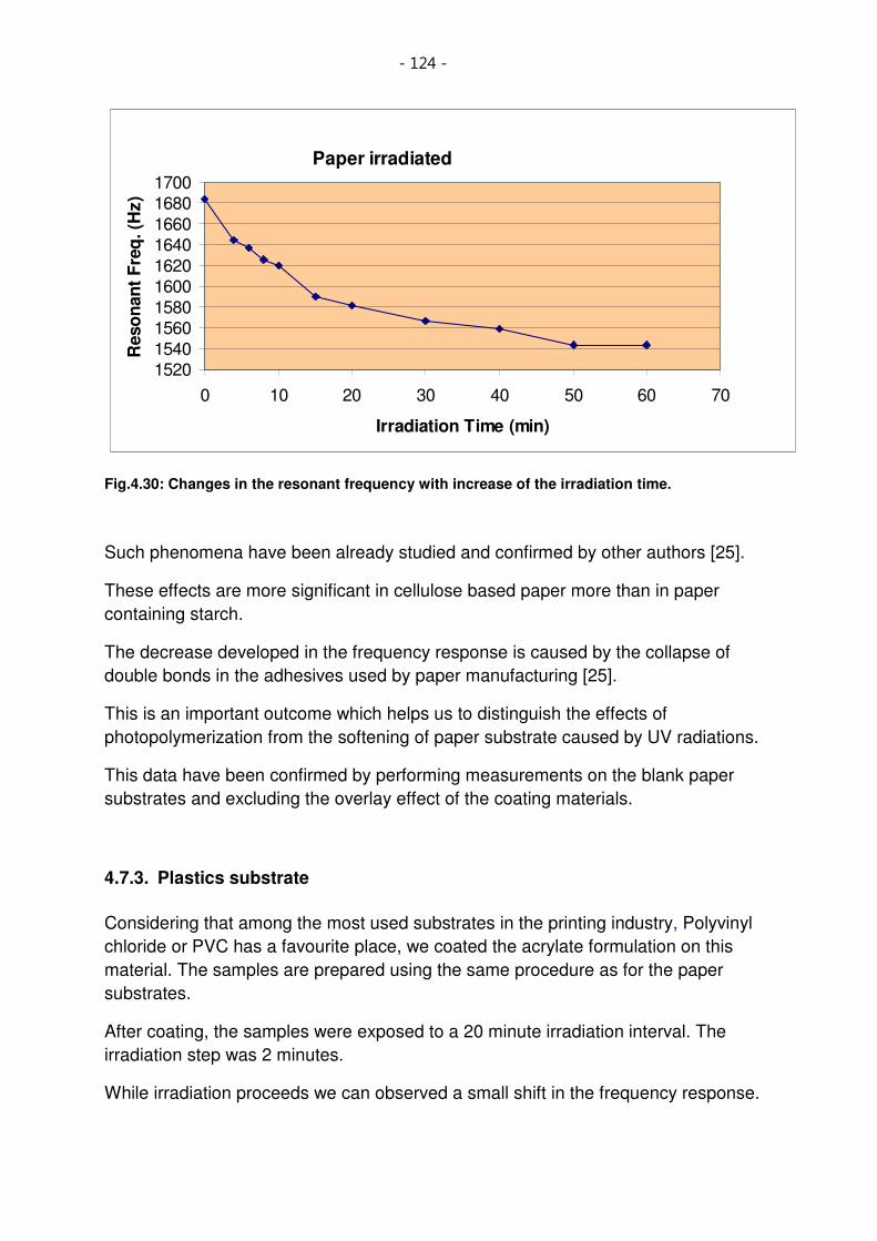
- 124 -

Paper irradiated

15201540

15601580

16001620

16401660

16801700

0 10 20 30 40 50 60 70


Reso

nan

t F

req

. (H

z)

Fig.4.30: Changes in the resonant frequency with increase of the irradiation time.

Such phenomena have been already studied and confirmed by other authors [25].

These effects are more significant in cellulose based paper more than in paper

containing starch.

The decrease developed in the frequency response is caused by the collapse of

double bonds in the adhesives used by paper manufacturing [25].

This is an important outcome which helps us to distinguish the effects of

photopolymerization from the softening of paper substrate caused by UV radiations.

This data have been confirmed by performing measurements on the blank paper

substrates and excluding the overlay effect of the coating materials.

4.7.3. Plastics substrate

Considering that among the most used substrates in the printing industry, Polyvinyl

chloride or PVC has a favourite place, we coated the acrylate formulation on this

material. The samples are prepared using the same procedure as for the paper

substrates.

After coating, the samples were exposed to a 20 minute irradiation interval. The

irradiation step was 2 minutes.

While irradiation proceeds we can observed a small shift in the frequency response.

- 125 -

As the crosslinking increased, the soft thin polymer film hardens and the frequency

registered just a small increase from approximately 1823 Hz to 1824 Hz.

A small shift is to be observed each time a new irradiation step was performed.

Fig.4.31: Changes in the resonance frequency for a sample coated on plastic substrate (PVC).

The changes registered in the resonant frequency of the plastic substrates are

obviously smaller as those monitored by the paper substrate.

In the Fig.4.31 we can see that the line shape of the resonant frequency is by far less

affected by the UV irradiation as in the paper substrate case. The amplitude’s line

shape presented the same sharp peak for all the investigated samples and a very

small increase in the amplitude’s value can be noted during the first 10 minutes

irradiation interval.

4.7.4. Mass loss

• The UV irradiation causes not only the ageing of the paper substrate, but

also generates evaporation of the humidity accumulated in the paper during the

storage.

• The substrate wetness, already discussed in Chapter 3, represents a

factor that affects the printability as well as the measurement signal.

To assert this assumption, we accomplished a series of measurements on blank

paper, stored under ambient conditions.

The investigated paper is commercially available (Chromolux) and had a thickness of

100 mµ . A strip, of 6x4 cm size, was used for our evaluation.

- 126 -

The paper strip was weighted on the microbalance and the value noted.

The paper sample was then exposed to irradiation for an interval of 10 minutes. The

irradiation proceeded in 1 minute steps. After each irradiation step the sample was

weighted and the value noted again.

The operation was repeated for the paper substrate coated with the acrylate

formulation (blue squares symbols in the Fig.4.32)

All experiments were performed in the clean room at constant temperature, humidity

and pressure conditions.

Fig.4.32: Mass decrease with increase cure time in the paper membrane.

There was a noticeable mass loss in the paper sample, obviously induced by the UV

irradiation. For the presented sample, it amounted to 1 mg, and it occurs after 1

minute UV exposure.

The mass loss in the coated sample was 1 mg, too, and was detected after 2

minutes UV irradiation time. Within the sensitivity of this simple experiment, the total

mass loss seems to occur more or less in the paper alone. There was no noticeable

mass loss in the coating.

The evaporation process and the correlated mass loss developed in the first minutes

of irradiation. After this time interval, the mass loss value rested constant for all

further irradiation operations. The evaporation process developed somewhat slower

in the coated paper with respect to the blank paper.

- 127 -

4.8. Measurements performed on samples printed by a MAN Roland printing

machine

To test our measurements technique, we investigated 53 different samples printed and cured in a MAN Roland printing machine.

One of the advantages of the samples prepared in a machine is the homogeneity of the coated film, defined in 2-3 µm thickness range. The second advantage was represented by the powerful UV lamps build in the machine which significantly shorted the cure time to a few seconds. The shortening of the irradiation time might eliminate the unwelcome effects of substrate aging by paper and also prevented secondary thermal effects in the plastic and aluminium substrates.

The printing process proceeded as follows: each different pigmented coating was

printed separately; even complicated patterns can be formed in this mode. After each

coating application, the sheet was underlying a cure procedure. For each one of the

four pigmentations (yellow, cyan, magenta, black) a specific UV dose was required

this means we needed to provide four independent UV lamps (Fig.4. 33). After the

printing machine, the printed sheets were further exposed to a final UV irradiation

dose. This last UV step was required because most of the sheets receive a clear

coating on top to increase their brilliance.

Fig.4. 33: Printing procedure in an MAN Roland printing machine. The coated sheets are

exposed at four UV operations (one for each pigmentation) and an additionally one for the clear

coating on the top.

- 128 -

The measurements were executed on three different paper substrates and one

plastic:

• Mega Gloss 150g/m³,

• Opti Gloss 150g/m³,

• Luxo Magic 150g/³

• Plastic (PVC).

Fig.4. 34: Changes in the resonance frequency of samples printed in a Man Roland printed

machine. Only very little change of the resonance frequency could be detected, whereas a

prominent change in the line shape and –integral is clearly seen.

The printing followed in the machine with two different sheet velocities (5000 and

10000 sheets/h) and for two different UV lamp doses 160 W/cm² and 2x160 W/cm².

As reference, an uncured sheet, exposed with same procedure as the cured

samples, has been considered.

In conclusion, the measurements showed an increase of the eigenfrequency by

increasing the UV doses. The peak in the frequency is strongly dependent on the

printing velocity. Sheets printed to a lower velocity (5000 sheets/h) and a lower UV

doses (160W/cm) reached same values in the resonance frequency as for samples

which were printed at higher velocity (10000sheets/h) and exposed to double UV

doses (2x160W/cm). This occurs considering same radiation time interval.

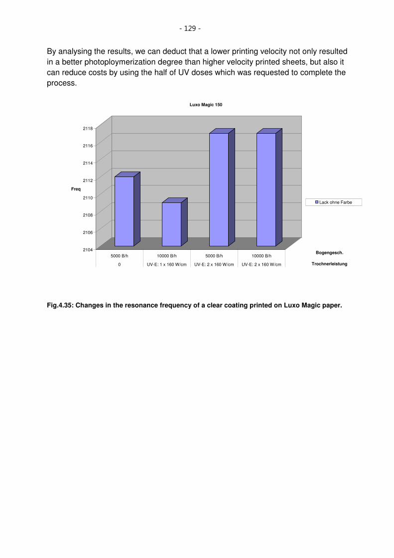
- 129 -

By analysing the results, we can deduct that a lower printing velocity not only resulted

in a better photoploymerization degree than higher velocity printed sheets, but also it

can reduce costs by using the half of UV doses which was requested to complete the

process.

2104

2106

2108

2110

2112

2114

2116

2118

Freq

5000 B/h 10000 B/h 5000 B/h 10000 B/h

0 UV-E: 1 x 160 W/cm UV-E: 2 x 160 W/cm UV-E: 2 x 160 W/cm

Bogengesch.

Trochnerleistung

Luxo Magic 150

Lack ohne Farbe

Fig.4.35: Changes in the resonance frequency of a clear coating printed on Luxo Magic paper.

- 130 -

2108

2110

2112

2114

2116

2118

2120

Freq

5000 B/h 10000 B/h 5000 B/h 10000 B/h

0 UV-E: 1 x 160 W/cm UV-E: 2 x 160 W/cm UV-E: 2 x 160 W/cm

Bogengesch ,

TrocknerLeistung

OptiGloss 150

Magenta - No Lack

Fig.4.36: Changes in the resonance frequency for a magenta pigmented sample.

2110

2115

2120

2125

2130

2135

2140Freq

- M agenta M agenta M agenta +

G elb

M agenta +

G elb

M agenta

(trockene

F läche)

x - x - x -

Farbe

Lack

M egaG loss 150

U V-E: 1 x 160 W /cm 10000 B /h

Fig.4.37: Changes in the resonance frequency of a magenta and yellow pigmented sample

- 131 -

4.9. Measurements in the time domain

The measurements in time domain were performed with the scope and subsequent

Fourier analysis to compare the results with the results obtained from the frequency

domain measurements.

The measurements were performed on three different substrates: paper, irradiated

paper and aluminium foil. As a sample coating we used a solvent based coating

which dried through emission of the volatile compounds. This coating was only

chosen to test the setup in general and to avoid the quite complex irradiation

process. Also, the evaporation of the solvent naturally induced a temporal effect

resembling the one induced by UV curing. The coating changed from ‘wet’ to ‘dry’

during solvent evaporation.

The measurements procedure was the same as for the experiments performed in the

frequency domain.

The substrate was clamped into the sample holder and after that the coating was

applied by spraying.

The paper membrane was clamped into the sample holder positioned horizontally

[Fig.4. 5]. This sample holder configuration was used to avoid the run down of the

liquid solvent based coating. At the same time, the perfectly horizontal position of the

clamp allowed an optimal access to the sample.

The dynamics of the drying process of solvent based coating on a paper membrane

can be seen in Fig.4.38.

Suddenly after the solvent based coating was deposited on the paper substrate, the

resonant frequency of the membrane decreased by about 70 Hz (fres = 1250 Hz), due

to the mass increase on the paper membrane.

As the coating begins to dry, as an effect of the evaporating solvent, a substantial

increase of about 120 Hz was detected in the membrane resonance frequency.

- 132 -

0,0

08

43,6

28

87,3

15

130,9

89

174,6

7218,3

5262,0

31

305,7

12

349,3

9393,0

74

436,7

52

480,4

38

524,1

13

567,7

98

611,4

73

655,1

61

698,8

36

742,5

23

786,1

97

829,8

76

873,5

57

917,2

38

960,9

21004,5

97

1048,2

82

1091,9

61

1135,6

44

1179,3

22

1223,0

08

1266,6

82

1310,3

69

1354,0

43

1397,7

22

1441,4

04

1485,0

84

1528,7

65

1572,4

44

1616,1

29

S1

0

1000

2000

3000

Eig

en

fre

qu

e

nc

y(H

z)

Time(s)

Solvent coating on paper

Fig.4.38: Dynamics of the drying process in a solvent based coating on a paper substrate. The

resonance frequency of the system decreases after applying the coating and, with the start of

the drying process, the frequency begins to increase again until a constant value is reached.

To further analyse this behaviour we performed the measurements with a solvent

based coating on an aluminium substrate. The aluminium substrate ensures that no

soaking or chemical modifications of the paper occur. Also, the aluminium reflectivity

is much higher as the one of plain paper which dramatically increases the signal to

noise ratio. The aluminium foil was clamped into the sample holder and the solvent

based coating was deposited on the substrate by spraying.

- 133 -

0,0

02

30,4

961,0

66

91,6

43

122,2

19

152,7

95

183,3

74

213,9

5244,5

25

275,1

305,6

76

336,2

53

366,8

3397,4

06

427,9

82

458,5

61

489,1

35

519,7

11

550,2

91

580,8

64

611,4

42

642,0

16

672,5

93

703,1

71

733,7

48

764,3

22

794,8

99

825,4

75

856,0

51

886,6

27

917,2

04

947,7

84

978,3

56

1008,9

34

1039,5

08

1070,0

85

1100,6

62

1131,2

39

1161,8

15

S1

0

2000

4000

Eig

en

freq

(Hz)

Time (sec)

Solvent coating on aluminium

Fig.4. 39: Dynamic of the drying process in a solvent based coating on an aluminium substrate.

The resonance frequency increases from a minimum of 1700 Hz to a maximum of 2700 Hz

corresponding to a final steady state.

After an initially decrease in the membrane resonance frequency (as marked in

Fig.4. 39), due to the solvent mass deposited on the aluminium substrate, an

increase of about 204 Hz is registered. The increase continues until the resonance

frequency reached a plateau (at approximately 2556 Hz) and remained stable for the

rest of the measurement.

The measurements performed with the solvent based coating showed two distinct

trends in the resonant frequency:

- immediately after application, the sample resonant frequency decreases,

because of the additional mass loading.

- once the solvent evaporated and the coating begins to dry, the sample

resonant frequency increases. This increase continues until the coating is

perfectly dried and the resonant frequency reached a constant value.

The acoustic resonator set-up was employed in two measurements variants:

- the frequency domain method

- the time domain method

The frequency domain measurements provided important information about the

extent of photopolymerization and the phase transitions during the curing process.

The collected data showed that the material vibration amplitude followed a decrease

- 134 -

with the cure time. The amplitude curves form presented similarly shape for all the

four investigated coatings and exhibits three regions:

The first region presents a gradually decrease in the amplitude for the first 20

to 30 cure minutes. Comparing to the storage modulus values, E’, measured

by dynamic mechanical analyzer, this region indicates the start of the cure.

The reaction is kinetically controlled and proceeds until the second region is

reached.

The second region is characterized of a dramatic amplitude decrease. The

values of the storage modulus and the peak in the loss modulus obtained by

the dynamic mechanical analyzer indicated that the gelation point was

reached. The continuous decrease of the resonant frequency suggested that

the frequency domain technique is sensitive to the changes in the viscosity or

modulus. The exactly gelation point can not be predicted and can be

overshadow by the vitrification.

After an irradiation interval varying from 50 to 65 minutes, depending on

sample’s pigmentation, the amplitude of the resonant frequency reached to a

constant value nevertheless the UV irradiation continues. This point indicates

that the crosslinking process is completed and corresponds to the vitrification

point measured by the dynamic mechanical analyser (DMA) in Chapter 6.

At this point the polymerization reaction becomes diffusion controlled and a

gradual change of material state from gel to a glassy state will occur. The gel-

glass transition is a dynamic transition and depends on the frequency

measurement interval and the cure time. The polymerization reaction undergoes

an important modification once reached the glassy state. This modification

appeared as an inhibition of the reaction kinetics even when a slowly diffusion

controlled reaction was present.

The frequency domain method measured the extent of polymerization reaction as

function of cure time with low temporal resolution. The start of cure, the gelation

and the vitrification point can be identified through the slopes registered in the

graph of resonant frequency as function of the cure time.

The time domain method was employed to investigate the reaction kinetic in real

time. The changes in the resonant frequency as a function of cure time were

observed and collected in real time. Thus, this technique provided precious

information about the degree of conversion and the polymerization rate.

Nevertheless, the method presently still has a few limitations. Those are

associated with the actual configuration of the measurement set-up and the

photodiode which, under intense irradiation, captured not only the reflected laser

beam but also part of the UV light. This led to a disturbed signal and to distorted

- 135 -

frequencies values. However, this phenomenon can be eluded by positioning the

photodiode on the rear part of the sample and using suitable protective screens.

- 136 -

5. SAW Sensor

5.1. Introduction

In the previous chapter, we have shown that the UV curing of a coating on paper, or other printable substrates, can be monitored by a change in the resonance behaviour of said substrate when operated in a resonator like setup. Here, we want to present a different and complementary technique, where the coating is deposited on a solid host substrate that is at the same time used as a monitor for the curing process. It relies on the presence of surface acoustic waves (SAW) on this substrate. The propagation parameters of the SAW are significantly altered during the curing process and can be measured with high precision. The substrate and the SAW form an acoustic sensor which can only be employed in a real life printing process separately. Because this acoustic technique is usually very powerful for the characterization of thin films, we wish to briefly outline the basics for the understanding of acoustic SAW sensors. Acoustic wave sensors are based, as their name indicates, on acoustic wave propagation and detection. Usually, acoustic wave sensors functionality relies on piezoelectric effects,which were discovered by the Curie brothers in 1880. The piezoelectricity can be defined as the induction of electrical charges by the exercise of a mechanical stress. This phenomenon is reciprocal, this means that by applying an electrical field to a piezoelectric material, this will be able to generate a mechanical wave which can travel through the substrate and could be at the end converted back into an electrical field. Those effects are caused by the Coulomb’s forces, which, by piezoelectric materials, reply to a mechanical deformation with the displacement in the electrical charges density of the material. Considering, that with a few exceptions, the piezoelectric materials are monocrystallin, the material will present a polar axis [26]. The characteristic of the polar axis by quartz, for example, are the asymmetric cells along that axis.

Fig.5.1: The cells structure by quartz and the piezoelectric effect.

- 137 -

The deformation of one cell, by applying a load along the direction of the polar axis, leads to the change of polarization due to reorientation of the positive charged Si++

and negative charged, 2xO-, of the quartz crystal (Fig.5.1). We define e, the proportional constant which relates the mechanical stress and the electrical field, induced by the polarization effect. Considering the anisotropy, typical for the piezoelectric materials, the constant e should be defined as tensor. The relation deformation-strain, valid for the purely elastic materials, can be extended to piezoelectric materials, considering the deformation as the result of an electrical charge [27].

∑∑∑== =

−=3

1

3

1

3

1 k

kkijkl

k l

ijklij EeScT

5.1

The electric charge density displacement or simply, electric displacement, is

correlated to the electric field through the electric permittivity tensor, ijε and depends

of the mechanical strain induced in the material.

∑∑∑= ==

+=3

1

3

1

3

1 j k

jkijk

i

jiji SeED ε 5. 2

The value of the elasticity tensor, ijc, depends on the electric charge applied to the

piezoelectric material, while the value of the piezoelectric coupling coefficient, ije,

depends of the mechanical stress. The use of the tensor analysis for the description of the piezoelectric effect, and the converse piezoelectric effect, prepared the base for the practical application of the piezoelectric materials as detection devices, particularly as acoustic wave sensors. An acoustic or mechanical wave, propagating through a material, will be affected by any changes in the material itself. These effects will influence the velocity and the amplitude of the propagating wave. Changes in material can be consequently monitored by measuring the frequency or phase of the waves and the recorded data can be then translated into physical quantities of interest for the material under test.

5.1.1. Piezoelectric Substrate Materials

There are few piezoelectric materials that are particularly suitable for manufacturing of sensors and devices: Quartz (SiO2), Lithium Tantalate (LiTaO3) and in the research field also Lithium Niobate (LiNbO3). Each of these materials exhibits their advantages regarding temperature changes, attenuation and wave propagation velocity [33]. There are various elements which are able to affect the sensor behaviour. One of the most important factors for the SAW propagation is the cut of the crystal which is selected for the sensor.

- 138 -

In Fig.5.2 we can see a quartz crystal and the possible directions cuts. Through an accurate choice of the crystal cut, the temperature effect can be minimized, and the stability of the sensor frequency can be improved. The temperature dependence of the resonant frequency in quartz crystal exhibits a parabolic behaviour for the DT, XY and NT cuts (Fig.5.13). An exception makes the thickness shear oscillator with AT-cut, where the temperature dependence follows the equation:

3

0

2

00 )()()( TTcTTbTTaf

f−+−+−=

∆ 5. 3

where the reference temperature 0T is fixed in this equation at 25°C. The changes in

the resonant frequency f∆ at a certain temperature T are function of resonant

frequency and temperature coefficients a, b and c. The constants a, b, c depend on the cut angle. Considering this typical values for the temperature dependence of the resonant frequency we can distinguish for each temperature range an optimal cut angle. The linear coefficient “a” results to be zero between 35°13’C and -49°C. AT and BT cuts exhibit weak temperature dependence (Fig.5.13) [27].

With the exception of temperature stable cuts, other cuts exist that show a strong sensitivity with the temperature. The literature gives as example the HT cut crystal

(∆f/Τ >> 103

Hz/K) [28,29]. Furthermore, sensor characteristics can be conveniently changed by deposing layers onto the piezoelectric substrate.

Fig.5.2: Photo of a quartz crystal and the different possible cuts.

Following this approach it would be possible for example, by choosing a layer with a wave velocity different from the velocity in the substrate, to transform substrate waves into surface operating waves. In Table 5.1 we show a list of the most used piezoelectric substrates employed for Rayleigh waves propagation. Each material is characterized of a different acoustic velocity, coupling coefficient, temperature and capacitance per unit length of finger pairs. Those parameters are essential for the stability of the measurement signal.

- 139 -

Table 5.1: Dependence of the characteristic parameters of quartz crystal of the specific cut. [30]

As it can be noticed, the highest coupling coefficient in this table belongs to the LiNbO3, usually employed in wideband SAW device. The coupling coefficient of the ST-cut crystal quartz is smaller, but having a low temperature coefficient of frequency makes it to be ideal for manufacturing of stable oscillators and devices, in association with its naturally narrow band.

The coupling coefficient pK represents the most important feature of a piezoelectric

substrate employed for sensor application. The square of the coupling coefficient represents the ratio between the stored, converted mechanical (or electrical) energy and the input electrical (or mechanical) energy. The coupling coefficient represents, therefore the efficiency rate for the conversion of the electrical energy in mechanical energy. The coupling coefficient can be determined, considering the follow equation:

||2||20

0

0

2

v

vv

v

vK e

elp

−=

∆= 5. 4

where 0v : is the phase velocity of the free surface

ev : is the phase velocity by short time overload of an electrical conductible

surface The LiNbO3 substrate has a high coupling coefficient and are, therefore suitable for broadband filter applications. The piezoelectric substrate used for the sensor employed in this work was a LiNbO3

Y-cut. This type of crystal allows the excitation of a Rayleigh wave along the Z-axis only, because of a cut perpendicular to the Y-(cut) axis.

Material Crystal Velocity

(m/s)

Coupling Coefficient (%)

Temperature TCF

(ppm/°C)

Capacitance per Unit Length of Finger Pairs

(pF/cm)

ST-cut quartz 3158 0.11 0 0.5

YZ LiNbO3 3488 4.5 94 4.5

128° YX LiTaO3

3992 5.3 75 5.0

77° YZ LiTaO3

3254 0.72 35 4.5

- 140 -

Fig.5.3: LiNbO3 128°C red Y-cut.

This characteristic together with the fact that along the X-axis no bulk waves can be generated makes the LiNbO3 Y-cut particularly suitable for sensors applications.

5.1.2. Fabrication of Acoustic Wave Devices

The IDT’s of the SAW components are usually made of aluminium because of its low density, its optimal substrate adhesion and its suitable transducer characteristics. A typical acoustic wave device consists of two sets of interdigital transducers. One transducer converts electric field energy into mechanical energy; the other converts the mechanical energy back into an electric field. In Fig.5.4 we can see a standard configuration of an acoustic wave sensor. Usually manufacturing uses photolithographic processes where metal layers can be deposited on accurately cleaned substrates. The target thickness of the transducer pattern is in the range of 50-200nm [30].

Fig.5.3: Photolithographic process for manufacturing of acoustic wave devices

More in details, the substrate is spin-coated with a photoresist and harded in an oven. A mask is then applied on the sensor and it allows exposing to UV light only the areas to be metalized (Fig.5.3). The exposed areas can be easily removed using a developing solution. The metal pattern so obtained on the sensor is called interdigital transducer or shortly IDT. The distance, as well as the position and the width of the fingerprint between the IDT’s, determine the performance of the sensor. As piezoelectric substrate, single crystal of quartz (SiO2), Lithiumtantalat (LiTaO3) or Lithiumniobat (LiNbO3) can be used (see 5.1.1). Through an accurate choice of the crystal cut (see 5.1.5) and the configuration of the IDT’s, the wavelength, as well as the wave type, can be defined.

- 141 -

The velocity of surface acoustic waves on piezoelectric substrates is in the range of 3000 to 5000 m/s. The frequency range corresponding to these values is among 10 MHz and 1, 2 GHz. Nevertheless commercially available SAW components usually have a frequency range from 80 to 500 MHz. Furthermore, the IDT’s can generate a wide spectrum of waves: transversal horizontally, vertically polarised as well as longitudinal waves: surface or bulk waves [31].

Fig.5.4: Typical configuration of an acoustic wave sensor

5.1.3. Acoustic Wave Sensors

As well as a variety of mechanical waves exists, there are to find a multitude of sensors or device acting by the specific wave type. There are two important categories of acoustic waves sensors called after the propagation type of the wave:

1. The bulk acoustic wave (BAW) sensors, where the acoustic wave propagates through the substrate.

2. The surface acoustic wave (SAW) sensors, where the acoustic wave propagates on the surface of the substrate.

The performances of the acoustic wave sensors are determined by the type of propagated wave. By analyzing the sample characteristics it is possible to choose the most suitable sensors.

5.1.4. BAW sensor

The most known BAW sensor is the quartz crystal sensor, which is basically composed of a quartz disc with two electrodes (Fig.5.5).

- 142 -

Fig.5.5: Schema of a quartz crystal sensor.

The design and the operating mode of the different quartz crystal oscillators are mainly the same. As sensors, they have to react with the attached medium in a specific way and meanwhile to rest protected, as electronics, from the medium itself. This type of sensors is also called QCM (quartz-crystal-microbalance) or TSM (thickness-shear-mode) sensors. By applying an alternating high frequency voltage to the electrodes, a shear deformation will be induced to the substrate. An additional mass loading on the substrate will generate a change of the resonant frequency of the quartz which is then monitored. Acoustic resonance happens when the thickness of the crystal disc is a multiple impair of the half wavelength. Usually, the resonant frequency is between 1 and 30 MHz. The first and most famous application of the acoustic resonators as sensors was developed and described in year 1959 by Sauerbrey [32]. He employed the quartz resonators as a ‘microbalance’ using the dependence of resonant frequency of the crystal on the mass charge. According to the resonance condition, the thickness of the quartz disc d

q (Fig.5.5),

must be half the wavelength of the acoustic wave λ q

2

q

qdλ

= 5. 5

The change in the frequency ∆f

q with respect to the change in the substrate thickness

∆dq

can be expressed as in equation 5.7, taking into account the propagation velocity

of the wave vq, which represents the product between of the wavelength

λ

q and the

resonant frequency of the quartz:

qqq f⋅= λν 5. 6

q

q

q

q

f

f

d

d ∆=

∆

5. 7

Similarly, we can derive the equation for the change of the quartz crystal mass ∆mq:

q

q

q

q

f

f

m

m ∆−=

∆ 5. 8

- 143 -

Sauerbrey also defines the term mass density MF

of a film, deposed on the crystal, as

the product between the film thickness dF

and the density ρF

of the film. Such relation

will have his validity assuming the film will be uniformly distributed on the electrodes surface; the film has to be thin and hard which means that the viscoelastic properties of the film sample have to be similar to those the quartz presents. This condition is known as the “gravimetric condition”.

FfF dM ρ⋅= 5. 9

The dependence of the frequency change ∆fq

with the mass density MF

is given by,

q

F

M

M

q

q

f

f ∆−=

∆ or

q

Fq

M

Mf

∆−=∆ 5. 10

From the equations (5.3) and (5.6) by substitution in equation (5.7) and ignoring the difference of the density between the quartz and the film sample, we obtain:

FFF

qq

qq McMff −=−=∆νρ

12 2

5. 11

where:

26 /1065,2 cmgq µρ ⋅=

scmq /1034,3 5⋅=ν

The equation 5.11 relates the dependence of the frequency change ∆f to a constant cF, which can be calculated from the quartz material properties and the mass density of the sample MF. The sensitivity of quartz resonators is directly proportional to the square of the oscillation frequency fq.

The sensitivity of the quartz resonator as mass balance is obvious in the eq. 5.11. As already mentioned, other factor which affects the acoustic resonance, in terms of acoustic impedance, due to sample viscoelastic properties, is the contact with other materials. In the specific case of gases the effect on resonant frequency can be ignored. By fluids we have to make instead some considerations; the propagation of the shear amplitude of the acoustic wave it is at the surface contact with fluids strongly attenuated. This attenuation is shown as function of the acoustic wave at the crystal surface in Fig.5.6.

- 144 -

Fig.5.6: Attenuation of an acoustic wave by propagation into fluids. The attenuation is due to the fluid viscosity.

Based on the consideration that the viscosity sρ and the shear modulus q

µ of the

quartz have characteristic values, Gordon and Kanazawa developed in 1985 an

empiric model [34], which correlated the viscosity sη and the density sρ of a fluid or a

chemical solution to the shift in the resonant frequency of the sensor.

qq

ssff

ρπµ

ρη0

2/3−=∆ 5. 12

5.1.5. Surface Acoustic Wave Sensor

The surface acoustic waves were discovered in 1885 by Lord Rayleigh who described their properties in his famous work [“On waves propagated along the plane surface of an elastic solid”] “It is proposed to investigate the behaviour of waves upon the plane surface of an infinite homogeneous isotropic elastic solid, their character being such that the disturbance is confined to a superficial region, of thickness comparable with the wavelength. .... It is not improbable that the surface waves here investigated play an important part in earthquakes, and in the collision of elastic solids. Diverging in two dimensions only, they must acquire at a great distance from the source a continually increasing preponderance. “[35] Rayleigh waves propagate in two dimensions (Fig.5.8) which means that such waves have two components in the sagittal plane: a component plane to the direction of propagation and a component perpendicular to the surface of propagation. The velocity of the acoustic wave propagation is slower at the surface than inside of a solid because of the lack of bonds at the solid surface, which is translated into a weaker restoring force in that area. This is the reason why the Rayleigh waves are not converted to volume waves but propagates at the surface [36]. The acoustic waves discovered by Lord Rayleigh had a first application in 1946, when Firestone and Frederick managed the piezoelectric excitation of a surface acoustic wave on a solid [37]. The first application allowed the detection of little cracks on the surface of the investigated material.

- 145 -

The simple way of excitation of surface acoustic waves through piezoelectric coupling on piezoelectric substrates becomes reality in 1965 with the design of the interdigital transducer (IDT) by White and Voltmer [38]. They created the basis for the development of surface acoustic wave components, especially for high frequency telecommunication engineering. For example, most of the RF filters in mobile phones are based on SAW devices. Similarly to the components for the bulk acoustic wave’s sensors, the components for surface acoustic waves sensors have to react with the sample, but in the meantime, they have to remain protected as sensitive electronics components from the sample. Differently to what happens in the case of bulk wave component, the mass charge creates a change in the velocity of the surface acoustic wave and therefore a shift in the resonant frequency. The measurement principle of the SAW sensor was also employed in this work and basically consists in the detection of any changes in the velocity and the amplitude of the acoustic wave in materials deposited on the sensor. These changes are generated as a result of the modified boundary conditions of the sensor surface. As already mentioned, acoustic wave are generated through an inverse piezoelectric effect. The material undergoes, through an applied load, a deformation. The load can be coupled, mechanically by means of a transducer or, electrically using a piezoelectric substrate. For a better understanding of operating mode of a surface acoustic wave sensor, we will describe the propagation of an acoustic wave through a solid.

5.1.6. Acoustic Waves in a solid

We can understand the motion and the propagation of an acoustic wave in a piezoelectric substrate when we asserted a correlation between the particles

displacement, iu of the substrate and the electrical field, iE

. We start with the motion of an acoustic wave in a non piezoelectric material and we assume that the material is composed of infinitesimal volume elements. Considering the second Newton’s law, where the product between the mass and and the velocity in a direction is the result of a force applied in same direction, and

assuming that the density of a volume element is ρ , we can define:

2

2

**t

udVdVaF i

ii∂

∂== ρρ 5. 13

The force iF represents the position gradient of the mechanical stress ijT

:

∑= ∂

∂=

3

1j j

ij

ix

TdVF 5. 14

By substitution of 5. 13 in 5. 14 we become the equation of motion for acoustic waves in a solid [27].

∑= ∂

∂3

1j j

ij

x

T=

2

2

t

ui

∂

∂ρ 5. 15

- 146 -

We defined above the two important equations for the piezoelectric substrates. Those equations make a relation between the electrical field, E the electric charge density displacement (electric displacement) D and the mechanical stress and strain, respectively. To describe the acoustic wave’s propagation in piezoelectric materials we should relate the particle displacement, u to the electrical field or to the electrical potential. By substitution of the tension tensor, T from the eq. (5.13) in the eq. (5.1):

ρ∂2

ui

∂t= ( c ijkl

∂Skl

∂x j

− ekij

l =1

3

∑k=1

3

∑j =1

3

∑∂Ek

∂x j

5. 16

The strain, S can be expressed as a function of the particle displacement using eq. (5.11). We can assume the relationship for the electrical field as stationary, considering that the propagation velocity of an acoustic wave is, substantially slower as those of an electromagnetic wave, and defined the electrical field as the gradient

of the electrical potential elΦ .

By substitution in eq. (5.14): Considering the axis symmetry of the piezoelectric material, the eq. (5.15) can be simplified to:

)(23

1

3

1

3

1

22

lj

elkij

j k l lj

kijkl

i

xxe

xx

uc

t

u

∂∂

Φ∂+

∂∂

∂=

∂

∂∑∑ ∑

= = =

ρ 5. 17

The same procedure can be taken by substitution of the strain tensor, S and the

electrical field expressed as electrical potential, elΦ in eq. (5.11):

)(2

1(

3

1

3

1 j

k

k

j

k

ijk

j j

eliji

x

u

x

ue

xeD

∂

∂+

∂

∂+

∂

Φ∂−= ∑∑

==

5. 18

Assuming, that the substrate is free of electrical charge, the gradient of the electric displacement will be zero:

0=∂

∂

lx

Di 5. 19

By introducing in the eq. (5.17) we become:

∑∑∑== = ∂∂

∂+

∂∂

Φ∂−=

3

1

23

1

3

1

2

(0k lj

kijk

l j lj

elij

xx

ue

xxε 5. 20

The eq. (5.16) and (5.19) presents a linear equation system for the acoustic waves equation coupled on a piezoelectric substrates. Theoretically, this equation system describes all waves’ propagation types. The analytical solution can be finding in the literature only for specific cases [39]

5.1.7. Acoustic waves propagation in solids

We will describe the propagation of the acoustic waves in solids and the correlation between the deformation and the displacement of the material, induced by the travelling wave.

- 147 -

In Chapter 2 we considered the relation between the deformation S and the displacement u∆ with the segment x∆ for a string. This is the one-dimensional case of the wave propagation equation. In the case of anisotropic materials, beside the deformation induced of the propagation of the acoustic wave, complementary deformations will arise. Those deformations are perpendicular to the direction of propagation of the wave. In this case the strain induced in the material, has to been extended to a tensor [39]:

)(2

1

k

l

l

kkl

x

u

x

uS

∂

∂+

∂

∂= with 3,2,1, =lk 5. 21

The index k,l indicates the axis )3,2,1( =ixi of a Cartesian coordinate system. Each

displacement of a particle in the material u leads to a deformation S which creates mechanical strain in the material. When the deformation is small, the strain is a linear function of the stress applied. In the one-dimensional case, the elasticity constant c is introduced as a proportionality term between the mechanical deformation and the induced strain. In

the general case, the mechanical deformation ijT is correlated to the strain, klS

through the elasticity tensor, .ijc

∑∑= =

=3

1

3

1k l

klijklij ScT 5. 22

with 3,2,1, =ji (Fig.5.7)

Fig.5.7: The stress tensor, ijT in the coordinates system 321 ,, xxx .

The tensor ijT consists of 9 terms. Considering that no torsion moment occurs, the

symmetry condition ijT jiT= has to be accomplished. It means that the stress tensor

has 6 independent components. Assuming, that the same symmetry condition is valid also for the strain tensor, the elasticity tensor should fill the condition [40]:

- 148 -

klijjiklijlkijkl cccc === 5. 23

The elasticity tensor count 21 of 81, independent components. The elasticity tensor can be defined, using only two indexes [39]:

mnijkl cc = 5. 24

with

llforkkn

lkforkn

jjforiim

jiforim

≠−−=

==

≠−−=

==

9

9

The literature gives the elasticity tensor for LiNbO3, which is the piezoelectric substrate used for our sensor device, as follows [41]:

210 /10 mNcij =

The elasticity matix for the LiNbO3 :

5. 25

By LiNbO3 rules the isotropic materials symmetry, thus the elasticity tensor can be simplified to 5. 26:

5. 26

The piezoelectric materials are not always isotropic. This condition is assumed, considering the isotropic character of the sensor coating material. The equation for

the elasticity tensor becomes the eq. (5.15). The coefficients 12c and 44c are, in this

case equivalent with the Lame constants, fλ and fµ

, used for the characterization of the elastic properties of sensor coatings.

fλ = 12c ; fµ = 44c 5. 27

- 149 -

5.1.8. Excitation of surface acoustic waves

The Rayleigh waves behaviour in a solid is very similar to those of the acoustic wave in an isotropic, no piezoelectric substrate. As mentioned, the Rayleigh wave has two components: a longitudinal wave and a perpendicular to the direction of propagation shear wave.

Fig.5.8: The Rayleigh wave consists of a longitudinal and a perpendicular to the direction of propagation component.

Meanwhile for the longitudinal component, the propagation path and the particle displacement follows in the same direction, the two vectors are orthogonally for the shear component. In a Rayleigh wave, the particles near to the surface exhibit an elliptical trajectory (Fig.5.9). The ideal Rayleigh wave has no horizontal polarised component, therefore no propagation or displacement exists along the x-axis. Another characteristic of the Rayleigh wave is the exponential decay of the oscillation amplitude from the surface along the negative y-direction.

Fig.5.9: Rayleigh waves surface propagation and the elliptical trajectory of the moved particles.

Assuming those characteristics, the solution for the wave equation along the y-axis in

the segment 0<y is a linear combination of 4 partial waves with the amplitude iA

and 4A [42,43].

)( Rtjyk

iiRiR eeAu

γωγ −= 5.29

with i=1,2,3

- 150 -

)(

4

Rtjyk

elRiR eeA

γωγ −=Φ 5.30

The factors, 1u to 3u , correspond to the particles displacement along the x, y and z-

axis. The displacement of the particles depends of the acoustic wave penetration depth into the substrate. As already mentioned, in the case of an ideal Rayleigh wave no displacement will be

registered along the x axis. The amplitude 2A is therefore zero. The different

amplitude are determinted by the coefficients, ik . The propagation factor, Rγ should

be defined as a complex factor.

jkR += αγ 5.31

The damping factor, α represents the decrease in the amplitudes of the propagating wave with respect to the propagation path of the wave (measurement unit=m-1). In the ideal case of a wave where no attenuation occurs, α =0. The wave number

k becomes 0k in case uncoated sensors substrate and can be calculated from the

angular velocity and the phase of the wave, propagating through the uncoated substrate [42]:

0

0v

kω

= 5.32

Considering (5.20) and the wave equation, we obtain an equation system which leads to the solution for the Rayleigh wave. Because of the complicated structure of the equations, the calculations are iterative and not analytical. This approach is largely discussed in the literature [43] and will be no further described in this work.

5.1.9. Sensor devices operating with Rayleigh Waves (SAW Sensor)

The energy requested to generate acoustic waves should be coupled by the means of a transducer. In the piezoelectric substrates, metal electrodes are used to create an electrical field in the substrate. The metal electrodes, disposed on piezoelectric substrates are called interdigital transducers (IDT). The IDT’s are made of plane metal electrodes which are interleaved like two combs (Fig.5.10).

Fig.5.10: Sketch of a SAW transducer on a piezoelectric substrate.

- 151 -

Adjacent metal strips belong to different electrodes and are called fingerprint. When an alternative voltage is applied to the two opposite electrodes of the IDT’s, an electrical field is generated between the fingers; the direction of this electrical field depends of the applied charge. The electrical field induces an alternating deformation of the substrate surface through the piezoelectric coupling. Let us indicate with “d” the distance between two adjacent IDT-fingers (Fig.5.10). The oscillation period corresponds to the double distance between two adjacent fingers, “2d”; the generated surface acoustic waves propagate perpendicularly to the IDT fingerprints in both of the piezoelectric substrate directions (Fig.5.10).. Their frequency, fSAW , is correlated to the excitation frequency according to the following equation:

fsaw=

SAW

SAWSAW v

d

v

λ=

2 5.33

where fSAW : the frequency of the surface acoustic wave [Hz]

vSAW: the velocity of the surface acoustic wave[m/s]

λSAW: the wavelength of the surface acoustic wave [m]

d : the distance between two adjacent IDT-fingers[m]

The piezoelectrical substrate used in our experiments was YZ-cut LiNbO3 , which has a velocity of 3488 m/s (Table 5.1), therefore for obtaining the operating frequency of 82 MHz and the distance between two IDT, by substitution in 5.32 should be 2d=42,53µm. The LiNbO3 parameters value requested to excite a Rayleigh wave are to find in the Table below [60]:

Table 5.2: Dependence of the characteristic parameters of LiNbO3 of the specific cut [60].

The distance between the metal electrodes and the configuration of the IDT’s on the piezoelectric substrate conditioned the electrical behaviour of the sensor. The two most important configurations are the delay line and the resonator mode. The delay line configuration consists of two IDTs disposed on the two opposite parts of the sensor substrate (Fig.5.11). The second IDT (the receiver) is placed on the piezoelectric substrate, at a certain distance to the first IDT (the transmitter), and has exactly the same geometrically sizes as the first one; the wave generated by the first IDT will propagate into the second IDT. Here the acoustic wave induces, through the piezoelectric effect, electric charges, which lead to an alternating high frequency voltage between the two IDT fingerprints (comb IDTs) of the receiver transducer.

Parameter YZ-cut 128° red

Surface normal y-axis 128° w/r respect to the y-axis

Propagation direction z-axis x-axis

Propagation velocity 3488 m/s 3980 m/s

Coupling coefficient 0,046 0,056

- 152 -

Fig.5.11:The delay line configuration in a SAW sensor

Because of the configuration of the excitation source, an IDT will generate always two opposite directional waves. The edge of the substrate reflects, in the delay line configuration, the propagating wave and leads, therewith to an unwelcome interference effect with the opposite propagating wave. This impediment can be overwhelmed either by tapering the substrate edge or by applying an acoustic absorber, which will damp the reflected wave at the edge. The absorber structure takes supplementary space on the sensor, therefore, in this work we renounced to this feature considering the employed sensor. Highly piezoelectric substrates like LiNbO3, need 40-50 fingerprints for each electrode, while low piezoelectric substrates employs up to 100 fingerprints. Responsible for the fingerprints number employed in

a sensor is the effective coupling coefficient pK defined by the eq. (5.4) and also the

impedance matching conditions for the external circuitry. The effective coupling coefficient is an indicator for the surface acoustic wave performance in term of excitation and detection. The second possible IDT configuration, with a lower attenuation, is the resonator configuration. In this case the electrodes arrays are arranged at both ends of the substrate. The waves transmitted from the transducer to the substrate edge are reflected back to the substrate middle from the reflecting electrodes arrays. In this way a standing wave is generated which has its maximal energy density in the middle of the piezoelectric substrate,

Fig.5.12: Surface acoustic wave sensor components: one port resonator (left) and two port resonator (right).

The attenuation and the bandwidth represent the most important features of a sensor component. The transmission is, in both described IDT’s configurations, strongly dependent of the IDT characteristics. It is actually mathematically connected to the IDT layout. For an unweighted, rectangular IDT as shown in the above figure, it turns

- 153 -

out that there is a relation between the number of fingerprints, N and the resonant frequency [45]:

0

0/

0 /

)/sin()( 0

ffN

ffNe

f

NfH

ffjN

π

ππ−= 5. 33

The functionx

xsin determinates the band behaviour of the transducer and it will show

a high number of secondary maxima if the number of fingerprints is as well high. The width of the main and the secondary maxima decrease with increase of the fingerprints number. Meanwhile the frequency range becomes larger due to the broader band. In the case of the resonator configuration, a standing wave will be generated because of the reflection of the specific reflector structures at the both ends of the piezoelectric substrate, Therefore, the band width depends not only of the band pass behaviour of the transducer, but also of the newly generated wave. In the resonator configuration the fingerprints occupies nearly the whole substrate surface(Fig.5.12), therefore the single resonance peaks belongs to bands which are narrower as the bands in the delay line configuration. The acoustic wave propagation velocity and the correlated transmission can be, in the delay line configuration, modified by coating the piezoelectric substrate with different materials. Some authors note that the mass sensitivity, for the sensors operating in the delay line configuration, increases with increase of the coating material thickness [27]. A coated substrate exhibits a slower phase velocity and therefore a bigger phase shift, in comparation with an uncoated sensor. That makes a coated sensor, operating in the delay line, more performing as the same, uncoated sensor. The clear coating samples were measured with a sensor operating in the delay line configuration and coated with a SiO thin film. The SiO coating protects the IDT’s and meanwhile has a lower damping factor as the uncoated sensor. The IDT’s of the SAW components are usually made of aluminium, which is well known as one of the best transducer materials because of its low density and its optimal substrate adhesion. Those components can couple with any sample deposited on the sensor surface. This will affect the amplitude and the velocity of the acoustic wave. Due to this characteristic the SAW sensors can monitor mass and mechanical properties. In a typical SAW sensor the acoustic wave has velocity approx.5 orders of magnitude less than the correlated electromagnetic wave. With an amplitude of about 10A° and a wavelength ranging from 1 to 100 microns, the Rayleigh waves are among the slowest waves to propagate in a solid [46].

- 154 -

5.1.10. Factors affecting measurements signal of a surface acoustic wave

sensor

For a better understanding of the signal operation mode we will describe the essential factors which affect the measurement signal. These factors will result evident as variables in the follow equation [47]:

*

*00

(1

GG

vm

m

vc

c

vvp

p

vT

T

v

vv

vs

s

s

s

∆∂

∂+∆

∂

∂+∆

∂

∂+∆

∂

∂+∆

∂

∂+∆

∂

∂=

∆σ

σ 5.34

Where, T : temperature [K] p : Pressure of the gas phase of the surface through the surface wave propagates

[Pa]

sσ : Conductibility of the surface through the surface acoustic wave propagates [S]

sc : Capacity of the surface through the surface acoustic wave propagates [F/m]

m∆ : Mass charge of the surface through the surface acoustic wave propagates [kg] *

G : Complex shear modulus of the surface through the surface acoustic wave propagates [Pa] When the coating film consists of a ideal elastic, non conducting film, the eq. 5.34 can be written [27]:

002

220

0

)(||||4

=

−⋅+⋅−=

∆

y

zz

fRfR

R

f

v

Evv

P

hv

v

vzy

ρρ 5.35

where PR represents the flux energy of the Reayleigh wave [J/m]. Considering that the elasticity tensor represented the ratio between the mechanical stress T and the strain S, the longitudinal strain modul Ezz can be written as:

33

33

S

TEzz = 5.36

If in the equation 5. 22 we introduce the Lame constants for the terms c12 , c44, by substitution in eq. 5.36 we will have:

)2

(4ff

ff

fzzEµλ

µλµ

+

+= 5.37

The terms| 2|yRv and 2||

zRv represented the surface particle velocity along the y- and

z-axis, repsectively. The Rayleigh wave has no component,vRx along the x axis. Introducing the constant below the eq. 5.35 becomes:

R

oyR

P

vvC

y

4

|| 2

0

1

=−= 5.38

- 155 -

R

yR

P

vvC z

4

|| 02

0

2

=−= 5.39

The particle’s velocity is proportional to the frequency, thus the constants above may be defined:

0

11

f

Ck = 5.40

0

22

f

Ck = 5.41

By substitution in the eq. 5.35 we obtain the equation, which describes the changes induced in the phase velocity of the acoustic wave by deposing a thin, non conducting film of thickness h and densitiy ρ:

5.42

The material constants 21 , kk are listed in the Table 5.3. The first term of the eq. 5.42 refer to the deceleration of the acoustic wave velocity through mass charge and explain so the negative sign of the material constants. The second term of the eq. 5.42 shows the increase of the acoustic wave velocity with the

shear modul µf. The term ( ff

ff

µλ

µλ

2+

+

), has for the most polymers materials a value between 0, 5 and 1, it means predominant will be the shear modulus of the coating material. The acrylate, and in particular the acrylate coatings belongs, with a modulus in the range of 106 Pa, to the relative soft polymers. The shear modulus of polymer materials increase with the frequency increase [62].

The parameter 0v

v∆ can be estimated using some practical considerations. In

paragraph 2, we will make some assumptions regarding the viscoelasticity of the coatings samples and their influence on the SAW propagation.

• Temperature:

The change in temperature is directly related to a change of the piezoelectric substrate elastic constant, which affect the velocity of the surface acoustic wave. The relation between the temperature and the propagation velocity of the surface wave depends on the substrate material and on the crystal cut. A.J. Bernot gives the following the temperature dependence for different piezoelectric substrate cuts (Fig.5.13).

)2

(4

)(0

02021

0 ff

fff

fffv

hfkhfkkv

v

µλ

µλµρ

+

+⋅⋅⋅−⋅⋅⋅+=

∆

- 156 -

Fig.5.13: Frequency shift as function of temperature for quartz oscillators for different cuts.

To minimize the temperature effect, temperature stable crystal cuts should be employed for the piezoelectric substrates. This characteristic can be achieved choosing the crystal cut which, in the specific operating temperature range, exhibits an inflection point (see Fig.5.13).

• Viscoelasticity

This paragraphs presentes a particular interest for our investigations, considering that the coatings’s formulation consists in a mixture of polymers (acrylate). The polymer materials were widely investigated as coatings for SAW sensors. Applying a polymer material applied onto the sensor surface, the resonant frequency of the sensor will registered a decrease, while the insertion loss of the sensor will registered an increase. Those effects are due to the viscoelastic character of the polymer film. Viscoelastic are those materials which present both elastically and viscous properties. When a load is applied to this kind of material, a component of the material will undergoes an elastically deformation, meanwhile another component will register a molecular rearrangement. Viscoelastic materials unlike purely elastic material loose energy when a load is applied and then removed. Usually, the viscoelastic material transforms the energy loss in other form of energy like in thermal. The acoustic wave coupled with the surface coating induces a high frequency deformation into this surface. A model to describe the effect of viscoelastic coatings film on the surface acoustic wave’s propagation can be finding in literature [44]. The coatings, which are considered as homogenous films with isotropic properties, are charcteriazed by the complex elastic modulus.

- 157 -

Fig.5.14: Shear deformation in a solid.

The complex elastic modulus is an important instrument for the description of the viscoelastic properties of the material. Fig.5.14 shows the shear deformation of a sample deposed on the sensor sensitive substrate. Through the oscillation the solid undergoes a shear deformation, which can be described using the complex modulus G*: G*=G’+iG’’ 5.43

The real part of the shear modulus, also called storage modulus, is the component where the load and the deformation are in phase. The imaginary part of the shear modulus, also called loss modulus, is the component where the load and the deformation are shifted at 90°C. The type of the coating film is responsible for the conversion of the acoustic wave mechanical energy into the coating. Here can be differentiating two regimes of the coating film: the acoustically thin and the acoustically thick regime. By the acoustically thin regime, the entire coating surface moves synchronously, meanwhile by the acoustically thick regime, the surface displacement is delayed with respect to the displacement of the bulk. The phase delay between the bulk and the surface of the film has to be considered.

- 158 -

Fig.5.15: Deformation of an: a) acoustically thin film and b) acoustically thick film, by the propagation of a Rayleigh wave.

In Fig.5.15 we can see the particle displacements along the z and y-axis. The

gradient zuz ∂∂ / leads to the compression and the extension of the film, meanwhile

the gradient zuy ∂∂ / leads to the bending of the film.

As criterion to distinguish the acoustically thin films from the acoustically thick films, the literature [42] suggests the index number RA, defined as:

||

00

G

hvAfR

ff

A

ρ= 5.44

where 0v : the phase velocity of the undisturbed Rayleigh wave

0f : the resonant frequency

fh : the film density, respectively the film height

A: material constant The material constant A depends on the substrate and can be calculated considering

the constants, 1C , 2C defined through the particle’s longitudinal and respectively

shear velocity:

21

2

22

CC

CA

+= π 5.45

where the longitudinal and shear velocities are related to the elastic constants through the following equations [80,81,82]:

- 159 -

ρ

lvc

2

11 = 5.46

ρ

2

44tv

c = 5.47

1211442 ccc −= 5.48

where lv represents the longitudinal progation velocity and tv the transversal

progation velocity, respectively.

Fig.5.16: The SAW induces a deformation in a) an acoustically thin coating film, b) acoustically thick coating film deposed onto the LiNbO3 substrate.

The material constants obtained by substitution of 5.45, 5.47, 5.48, 5.46, in eq. 5.40 and 5.41, are listed below.

Table 5.3: The constants 0v , 1k , 2k used in the eq. 5.53.

YZ cut LiNbO3 Value

Propagation velocity, 0v 3488 m/s

Density, ρ 4642 kg/m³

1k -6,86 * 10-12 ms²/kg

2k -3,16* 10-12 ms²/kg

- 160 -

The material constant A estimated for the YZ cut LiNbO3 substrate, where no displacement followed along the x axis, we obtained obtained:

6,1~A

We obtained, 163,0 <=AR , therefore the film may be considered acoustically thin. It

means the coating film moved synchronously with the surface acoustic wave. The SAW operating frequency was 82 MHz, which corresponds to a wavelength of λ= 42,53 µm for a coating film of 2 µm.

Therefore the coating thickness, fh << λ, accomplished the conditions of a thin film

model. In the same time, considering that the shear modul of the coatings is in the range of

|| G ~ 610 , which classified those films among the soft polymers and considering that

the coating were applied onto a polypropylene film, which brought an additional layer of soft polymer, we will calculate the damping of the coating film using also the acoustically thick model. The || G values were taken from the DMA (Dynamic Mechanical Analyzer)

measurements (Chapter 6) and from literature materials tables. The literature [27,39] gives a model to estimate the changes in the damping of a Rayleigh wave through a ideal elastic, non-conducting film:

0

2

0

220

0

.||.||4

=

−+−=

∆

y

zz

fRfRy

R

f

v

Evv

P

hv

v

vz

ρρ 5.49

where 0v : the phase velocity of the undisturbed Rayleigh wave

0f : the resonant frequency

fh : the film density, respectively the film height

PR: the energy flux of the Rayleigh wave [J/ms].

From Fig.5.15, it may be seen that zzE represents the ratio between the mechanical

stress T of the film and the strain S, in the wave propagation direction. The bending

moment, zu y ∂∂ / can be neglected. Thus, for the longitudinal strain, considering eq.

we can define:

33

33

S

TE zz = 5.50

The strain modul can be defined also using the Lame`constants [61] ( Fig.5.27):

+

+=

GK

GKGE zz

43

34 5.51

Considering that by mostly polymers materials |K| >> |G|, eq. 5.51 may be simplified to:

GE zz 4= 5.52

Thus, the changes in the wave’s velocity and in the damping can be written:

0202021

0

''4).(

v

Ghfkhfkk

v

vfff ⋅⋅⋅−⋅⋅+=

∆ρ 5.53

- 161 -

2

0

02

0

''4

v

Ghfk

kf ⋅⋅⋅−≅

∆α 5.54

The shear modulus depends on the temperature and on the operating frequency. We learned above that a thin film moved synchronously with the travelling acoustic

wave. Furthermore, when 1<<AR , thick films behave in the same mode as thin films.

The damping factor and the SAW propagation velocity showed a linear dependence on the film thickness. In the Fig.5.17 and Fig.5.18 we can see the dynamic of the damping factor as function of the film thickness. The Fig.5.17 represents the behaviour of a polymer coating film with small loss modulus (~106 Pa, as in the materials table listed). The damping increase with the increase of film thickness and reached a sharp maximum, which is due to the small value of the loss modulus. In the Fig.5.18 the value for the G’’ were conformed to the experimental won data (~108 Pa as measured for the acrylate coatings). The results are obtained consider a coating film (Polyacrylat G’= 4, 6 108 Pa and G’’= 2, 3 108 Pa) with the density, ρ=0,25g/cm³ [76, Chapter 6]. The SAW operating frequency was taken 82 MHZ for an YZ cut LiNbO3 substrate and the material (LiNbO3) constants are listed in Table 5.3.

Fig.5.17: Damping behaviour as function of the film thickness for a coating film. The model represents a thin coating film.

- 162 -

Fig.5.18: Damping behaviour as function of the film thickness for a coating film. The model represented a thin acrylate coating film.

For the acrylate films, the damping increases with the increase in the film thickness, whereby the curve form becomes wider and the maximum is reached at approximate 2 µm. Therefore, the power coupled in the film registred its maximum.

5.2. Experimental

We employed the SAW device to detect the transitions undergoes in coatings samples under UV irradiation. In particular, the scope was to find out if the three main regions, which are characteristic for the photopolymerization process (start of the photopolymerization, gelation and vitrification), can be identified. Another topic was to determine a possible correlation between the attenuation of the velocity of the acoustic wave and the crosslinking, in order to consider the SAW sensor an alternative method for measuring the photopolymerization under laboratory conditions. As reference method we used the DMA (dynamic mechanical analysis), whose measurements principle is largely described in Chapter 6. The changes in the elastic modulus were evaluated as function of the irradiation time. The response of the sample on the applied load gave us the storage and the loss modulus of the acrylate sample and helped to identify the gelation and the vitrification point as a function of temperature (Fig.5.33). The samples consisted in commercially available multifunctional acrylate coatings in two formulations: pigmented in the four specific UV colorations (magenta, cyan, yellow and black) and a clear or unpigmented variant of the same formulation. The pigmented formulation has a higher viscosity in comparison with the clear formulation (viscosity DIN 4, 23° C: 60 ± 5s for pigmented coatings to viscosity DIN 4, 23° C: 40 ± 5s of clear coatings, from the material data sheet).

- 163 -

5.2.1. Sample preparation

We investigated two types of samples: a pigmented and a clear multifunctional acrylate coating. Whereas the clear formulation presented a gel like texture, and therefore was easy to apply, the pigmented formulation had a high viscous texture and was very difficult to apply by common laboratory methods. The pigmented samples were printed in a manroland printing maschine (see Chapter 4) and then brought in a “black box” in labour. The printed samples were homogenous, plane and their thickness ranged from1 to 2 mµ .

The clear coating samples were prepared at the beginning of our investigations, using the spin coating method at 30.000 rotation/min for 3 minutes time interval. The samples were measured after the UV irradiation gave a thickness in the range from 1 to 2 mµ .

The samples are coated in the laboratory using a minicentrifuge built with the help of the lab technical personal. The centrifuge is constituted of a very simple bowl with inside a sample holder that can rotate when an voltage (12V) is applied.

SAW sensor

Holder

Sample

Spin-coating

bowl

12V

Fig.5.19: Spin-coating bowl for sample preparation.

When the voltage is applied to the bowl, the rotation movement distributes the low viscousity coating as thin film on the piezoelectrical substrate. The obtained film was thin, but not uniform. One of the main disadvantage of this methode was the clamp holder; the tight grips of the holder damaged the thin and delicate LiNbO3 substrate of the sensor. As consequence, another method to prepare the samples was considered, using a combined drop method. We deposed a drop of the clear formulation directly on the piezoelctrical substrate and press to obtain a thin, uniform film. Because the formulation contains no solvent, that eventually needed to damp, it was possible to start the measure directly after the sample preparation. Similarly to the drop method, even in this case an exact determination of the film thickness was not possible. The samples were prepared by deposing permanently the same drop mass at the same condition. To have a real value, we prepared by the same method a specimen reproduced on a thick polypropylene substrate. The thickness calculated from the substrate geometry and coating mass gave us a thickness in the range of cca. 1-2 mµ .

- 164 -

5.2.2. SAW Sensor

The measurements are made with two type of sensors, both designed and assembled at the Chair for Experimental Physic I. On this substrate were brought, through an optical litographic process, the IDT’s fingerprints. (Fig.5.3).

Fig.5.20:The chip bonded on a sample holder.

The piezoelectric substrate was fixed on a sample holder with more contact pins. (Fig.5.20). The contact between the pins and IDT’s is done by thin wires. The wires were bonded at both ends using the ultrasonic welding, a very popular technique for bonding thermoplastics. A high-frequency ultrasonic acoustic vibration is applied to the work piece being held together under pressure to create a solid-state weld. The samples are positioned on the chip, fixed in the holder and connected to a network analyzer (Fig.5.21). The samples are irradiated with a UV mercury arc lamp (HBO100 lamp with 100W) through a 10x microscope lens.

Fig.5.21: Photo of a sample on the chip.

The measurements were performed with a Network Analyzer ZVC from Rhode and Schwarz, which gives a continuous signal in the frequency range 9 kHz-1.1GHz. The network analyzer has two available ports (Port1 and Port2), both can be used as in- and output. At the output we detected a high frequency signal with varying frequency (linear sweep). This signal was measured at the input with respect to the output

- 165 -

signal. Measurements may be performed in reflexion (input and output at the same port, respectively S11 or S22) or in transmission mode (input and output at different ports, respectively S21 and S12) like in Fig.5.22, whereby real and imaginary term or amplitude and phase respectively, can be measured.

Fig.5.22: Schema of the set-up for transmission measurements.

The network analyzer is useful to simplify the detection of changes in time, frequency or phase. These measurements are recorded with automatically tracking, and measurements within broad frequency intervals are possible. For an IDT distance of approximate 5 mm we obtain, considering the specific LiNbO3 velocity (see Table 5.1), 1 to 2 µs runtime. This results in a substantially delay of the surface acoustic wave’s signal with respect to the 100 ns typical cable runtime and eliminates undesidered effects to the measurement signal. A generator with pulse, frequency and amplitude variable, generated the surface acoustic wave for all undertaken measurements. Signal amplitudes were measured, with respect to acoustic wave amplitudes, using a LeCroy 9400 oscilloscope.

For a better understanding of the results a few parameters and their units have to be discussed.

5.2.3. Estimation of the SAW amplitude and damping from the transmission

measurements

The damping factor and the power are usually expressed in the high frequency engineering in logarithmical units.The power in dBm can be obtain from:

P (dBm) = 10log10 (mW

WP

1

)() 5.55

Similarly, the transmission can be expressed as:

T (dB) = 10log10 ( ))(

)(

WPtr

WPin 5.56

- 166 -

In the experiments performed on the pigmented samples the transmission S21 was measured through the sample. Using the equation below, we can estimate the damping of the acoustic wave from the measured transmission factor [79]:

el

dBS

log10

][21

⋅⋅−=Γ 5.57

where l represents the length of the sample film along the wave path S21 represents the relative amplitude of the transmitted signal. The damping Γ is defined as the loss in the acoustic wave along the z axis:

zeIzIΓ−= 0)( 5.58

For the clear coatings samples we estimated the SAW amplitude considering that the surface acoustic wave represented the transmitted power. This model was defined by Datta [45] and said that the SAW power, Psaw is divided by the IDT’s aperture, d:

2/1

0

)1

2(d

P

y

SAWSAW λ=Φ 5.59

where Φ is the surface electrical potential and y0 is the acoustic admittance. From the equations 5. 21 and 5.59 we can related the SAW amplitude to the displacement along the x,y and z-axis and estimate the SAW transmitted power as proportional to the amplitude square.

5.2.4. Measurements on pigmented coatings

The pigmented samples are investigated using an YZ-cut LiNbO3 chip with one delay line for each pair of IDT. The samples were printed in a Manroland printing machine and were coated on polypropylene substrates and finally cut in 4mm width stripes. The samples were deposed perpendicular to the wave propagation direction and pressed with the coated surface in direct contact with the chip (Fig.5.23). The delay time was of approximate 1 µs. The transmission S21 measured on the sensor without sample was -18 dB. The sample film brought an additional damping of 11 dB.

- 167 -

Fig.5.23: The UV coatings were printed on a polypropylene layer. The coated side was pressed onto the SAW sensor and positioned between the two IDT’s. S

The resulting two-layer (coating+polypropylene film) structure of the sample once applied on the sensor device was irradiated through the polypropylene layer with a HBO 100 W mercury lamp from Osram. The damping measurements resulted in an increase of the damping for all four pigmentation, whereby some pigment typical characteristic can be observed. To eliminate times delay effects, for each colour were made two measurements:

• Sample1: irradiation started immediately after application on the sensor device (black line on the graphs).

• Sample2: irradiation started approximate 50 s after application on the sensor device (red line on the graphs).

The red pigmented coating showed, directly after turn on the UV light, a sharp drop in the damping, followed within few seconds of an increase. This signal goes into saturation at -3 dB with respect to the start value (approximate 0, 75 dB/mm). The sample 1 and sample 2 showed the same curve shape, the only characteristic is the time delay for sample 2 (Fig.5.24).

Fig.5.24: Magenta samples on thin polypropylene foil irradiated through the substrate.

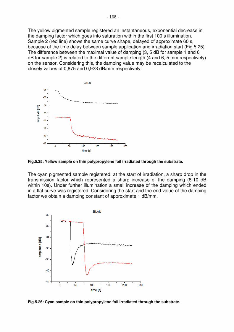
- 168 -

The yellow pigmented sample registered an instantaneous, exponential decrease in the damping factor which goes into saturation within the first 100 s illumination. Sample 2 (red line) shows the same curve shape, delayed of approximate 60 s, because of the time delay between sample application and irradiation start (Fig.5.25). The difference between the maximal value of damping (3, 5 dB for sample 1 and 6 dB for sample 2) is related to the different sample length (4 and 6, 5 mm respectively) on the sensor. Considering this, the damping value may be recalculated to the closely values of 0,875 and 0,923 dB/mm respectively.

Fig.5.25: Yellow sample on thin polypropylene foil irradiated through the substrate.

The cyan pigmented sample registered, at the start of irradiation, a sharp drop in the transmission factor which represented a sharp increase of the damping (8-10 dB within 10s). Under further illumination a small increase of the damping which ended in a flat curve was registered. Considering the start and the end value of the damping factor we obtain a damping constant of approximate 1 dB/mm.

Fig.5.26: Cyan sample on thin polypropylene foil irradiated through the substrate.

- 169 -

As a demonstration that the damping decreased only under irradiation, we recorded the dynamic behaviour of sample 2 with the cyan pigmentation after turn off the UV light.

Fig.5.27: Dynamic of photo polymerization on cyan sample on thin polypropylene foil by turn-off of the UV light.

As in the Fig.5.27 to see, the transmission registered, after turn off the UV light, a sharp drop, but within few seconds increased to initial value (before turn off the UV light). This behaviour is very similar to those occurred by turn on the UV light, thus the changes in the transmission and damping are directly related to the irradiation process (Fig.5.27). The sample initial state (before the start of irradiation) cannot be reproduced, what underline the SAW device sensitivity toward the polymerisation process. The Fig.5.28 shows different frequencies spectra recorded at different irradiation stages with the scope to prove that the detected effects are a result of polymerisation process and not a consequence of the time delay in the measurements which may induce a shift in the frequency spectrum.

- 170 -

Fig.5.28: Frequencies spectra taken at different moments with respect to the irradiation.

In paragraph 5.1.12 we learned that three parameters are responsible for the changes registered in the SAW propagation by deposing a coating film onto the sensor device. Those parameters are the damping factor, the wave vector and the complex propagation factor. The literature [52] shows how to calculate a theoretical

model, which defined the relative changes in the propagation factor, Rγ . The

propagation factor is related to the damping factor through eq. 5.31 and shows the effect of a coating film deposed onto the sensor surface. The experimental data reveal that the curing of a thin acrylate film applied onto the sensor device leads to an increase in the damping factor of approximate 1 dB/mm with small difference for each colour. Because the damping factor depends on the SAW path length, we considered this in our results. The damping factor should be recorded for each colour as function of the film thickness and of the cure time.

5.2.5. Measurements on clear coatings

Measurements on clear coating were made on a second SAW sensor, already in use for microfluidic experiments at the Chair for Experimental Physics I. The SAW sensor consisted of a sample holder with 12 contact pins (cantilever) sold on a board. The board was positioned between two metal plates of aluminium and formed the connecting part. Both plates were then grounded and protected the circuit board. The top plate had as well eight boreholes for the insertion of high-frequency connections (Fig.5.30). The sample holder instead was made of copper and immediately below is positioned a Peltier element. The Peltier element was employed to regulate the sample temperature during the irradiation.

- 171 -

Finally the samples are deposited on the sensor chip and irradiated using a UV mercury arc lamp from Osram. The changes in the amplitude of the acoustic wave were recorded as function of irradiation time.

.

Fig.5.29: Samples are irradiated with a HBO100 mercury arc lamp integrated in an objective microscope.

The viscoelastic changes in the correlated phase transition were investigated and described in Chapter 6. The relaxation process and the glass transition temperature point were detected using DMA (Dynamic Mechanical Analysis) measurements. The chemical changes during the photopolymerization process and the degree of cure has been studied by real-time FTIR (see Chapter3) and used as reference method. The data from the SAW sensor were evaluated using a National Instrument Lab VIEW equipment control platform. Both the measurement output file and the source file were not an ASCII data, but a block-diagram similarly to an electronic circuit. The data flows in the wires which started at the “entry-nodes”. Entry and end function nodes run under “sub-vi’s” and ended in the indication nodes. The entry and end nodes on the block diagram correspond to the front panel. The encoding in block diagram makes easy the correlation to the data flow and provides an efficient coding without a real text program. The software gathers in real-time the amplitude of the acoustic wave versus time from the SAW sensor. As real-time we mean one scan every ten seconds. The program takes the data from the network analyzer, plot the amplitude versus time and save the numerical data to a log file. Similarly to pigmented samples, measurements for clear coating samples were executed with same instrumentation setup.

Fig.5.30: SAW Sensor; the surface is protected with a SiO2 layer. A thermocouple and a Peltier element are attached to the sensor.

- 172 -

The sample was applied directly onto the sensor surface, whose conversion rate and mechanical properties were well known. A high frequency electrical pulse (f=82MHz, P=-39.47 dB, Mag=10dB for the sensor without sample) was applied to one of the interdigital transducers and than converted into a surface acoustic wave. After being propagated into the sample, the acoustic wave was picked up by a second transducer, where the transmitted signal could be analyzed in terms of amplitude and phase shift with respect to the incoming signal. The photopolymerization process began with the irradiation start. The coating photoinitiators generated free radicals under irradiation that combined with the multifunctional monomers of the formulation and built a three dimensional polymer network. This is an irreversible process that develops at very high rates. As we can see in Fig.5.31 the increase in the amplitude of the acoustic wave was already significant by the start of the UV irradiation. As the irradiation continued, the photochemical reaction went forth at high energetic level, causing reduced ion mobility due to crosslinking and opposing to the exothermic temperature effect. By the transition from the liquid to the solid phase, the sample registered an increase in the amplitude and in the meantime a decrease in the damping loss. The phase transition and the changes in the mechanical properties of the sample were investigated through the dynamic mechanical analysis and are discussed in Chapter 6. The relaxation process is correlated with motions of great chain segments of polymer, therefore with large changes in the modulus and viscosity of the polymer. The first relaxation and the transition temperature associated to this point are known respectively as α transition and Tα. This point is usually indicated as the crossover point in the real and imaginary term of elastic modulus [55]. A distinction has to be made between Tα and Tg. While Tα represents the temperature where the dyndmic glass transition started, Tg represents the static glass transition temperature point [54]. This distinction is not always clear in literature, many authors note Tg as Tα and vice versa. To avoid further confusion we assume Tα as the point where begin the formation of the new polymer (gelation point) and Tg as the point where the new formed polymer undergoes the transition from the gel to the glassy state (vitrification point). We assume that Tg is, in the DMA measurements, the peak in the loss tangent measured as function of temperature. However there are authors that indicate the Tg as the peak in the loss modulus [56]. The elastic modulus of the new formed polymer is strongly dependent of its density and increases with increase of the irradiation time (see Chapter 6). The acoustic measurements show an increase in the amplitude of the acoustic wave with increasing of irradiation time and therefore with a higher elastic modulus (Fig.5.31).

- 173 -

Fig.5.31: Kinetics of the photo polymerization process for an acrylate clear coating system as being detected by a SAW sensor.

The polymerization process of a 2 µm thin coating layer causes a change in the SAW amplitude of 25 dB .

Fig.5.32: Dynamic of the photo polymerization process for a different Acrylate clear coating sample as being detected by a SAW sensor. The moment when UV light is switched on is marked in the figure above. The measurements performed on the clear coatings showed two regions of interest in the acoustic wave amplitude. Shortly after the start of irradiation, the SAW amplitude registered a sharp increase for the first 12 ms. After this time interval the amplitude of the acoustic wave registered a minimal increase and after further 2 ms goes the signal goes into saturation. This amplitude value remains unchanged also in absence of irradiation. The measurements in all investigated clear coating samples showed same curves profile. The increase in the irradiation time showed an increase in the SAW amplitude and therefore a decrease in the acoustic wave attenuation. Two distinct regions can be considered, in the first one the SAW amplitude increases almost linearly with the irradiation time, in the second region the SAW amplitude goes into saturation, remaining practically constant. The transition point between the first and the second region is indicated by the onset in the SAW amplitude. Between the first and the second region the SAW amplitude registered an increase of cca 10dB in cca 12ms.

- 174 -

Fig.5.33: Phase transition in a clear coating sample measured in clamp tension film at 1Hz and 5°C/min.

Correlating with the DMA measurements, we can recognize that the start of polymerization and the static glass transition temperature point can be detected with the SAW sensor. The increase in the SAW amplitude is correlated to the increase in the elastic modulus. Some authors [57] report about a decrease of the SAW frequency with the decrease of the polymer modulus. Martin and Frye reported a SAW frequency increases due to

polymer film viscosity decreases.

The linear increase in the transmission factor in the first region corresponds to a decrease in the damping and is due molecular rearrangement that follows at low energetically level. The chain segments of the polymer presents in this phase a high mobility, therefore only a few of them can find the most energetically convenient configuration. This phase corresponds in the DMA measurements to the temperature region under

the T α (=27.8°C for a clear coating formulation). The dynamic glass temperature is

sensed as an onset in the transmission factor of the surface acoustic wave. Once the first relaxation transition point is reached no noteworthy phenomena aroused in the surface acoustic wave behaviour. The transmission factor showed a minimal increase, correlated to a decrease of the damping factor and ended than in a flat curve. After the dynamic transition point is reached, the damping factor remains for the rest of the process at a constant value. The acoustic energy can be dissipated through the relaxation process in this region which is defined as the interval between the dynamic glass transition temperature

T α (=27.8°C) and the glass transition temperature Tg (=45.08°C).

The polymer chains can rearrange themselves in short time in energetically, advantageous configuration. Once this configuration is reached no significant events occurred; the polymer becomes rigid, because the polymer chains are limited in their mobility and the

- 175 -

relaxation is blocked. For the clear coating formulation an increase of cca 10 dB between the liquid state and the glassy state is registered. The measurements on clear and pigmented coatings showed that the application of a system, consisting of a thin coating film and a polymer (polypropylene) layer onto the SAW device, affects substantially the transmission behaviour of the acoustic wave. The transitions induced through UV irradiation into the coating samples can be related to the damping of the acoustic wave and were recorded as an exponential decrease in the transmission. There are a few considerations to be made regarding the SAW sensor measurements on the pigmented coatings. Whereas the clear coating formulation was relative easy to be shaped as a thin, uniformly film, the pigmented formulation could be satisfactory processed only in a printing machine. The high viscosity of the formulation does not allow a uniform coating distribution and especially in these measurements the homogeneity of the sample as well as the thickness plays an essential role. The other great limitation, while handling coating formulation on SAW sensor, was the process of cleaning the sensor when removing the sample. The clear coating could be removed with common solvent as isopropanol, however the pigmented formulation was very though to remove not only by isopropanol, but also by stronger solvents as acetone. We employed instead typical production solvent to obtain a clean sensor surface. Unfortunately during this cleaning process part of the bond wires were also being removed. After each measurement of a pigmented sample a new wire rebond on the sensor surface was required. Another aspect to be considered, by measurements with SAW sensors, is the sample deposition on the chip surface. The adhesion of the sample has a significant influence on the velocity of the acoustic wave and on the correlated amplitude and damping factor. As consequence,the polypropylene samples are to be hardly pressed on the chip surface to assure an intimate contact and therefore good coupling between the sample and the sensor.

- 176 -

6. Dynamic Mechanical Analysis

6.1. Basic principles

When a force is applied to a material, the response is a deformation. Depending on the elastic properties of the material, the response gives insight into the mechanical structure and possible anisotropies of the sample under investigation., A typical measurement of the elastic or plastic properties of the sample is made by applying a known force and monitoring the changes in the geometry (deformation) of the sample. To increase the sensitivity, very often the force is applied not statically but instead an oscillating, sinusoidal force is inducing the deformation. Also, the force is applied in various directions along the sample to gain insight into the elasticity tensor components. This deformation can be measured using dynamic mechanical analysis (DMA) techniques. It thus can also represent an independent method to get access to the UV curing behavior of the samples investigated in this work. The results can then be compared and brought into context with the data presented in the previous chapters. Dynamic Mechanical Analysis is a technique which permits to study the three main regions in a curing sample. This is achieved with the analysis of the viscoelastic response properties of the material under stress (see Fig.5.1).

Fig.6. 1: The sinusoidal stress and corresponding strain ε response for a linear viscoelastic material. The applied stress and the material response do not coincide, and the phase angle δ is the difference between the two curves.

The most important transitions in a curing material correlated with changes in the viscoelastic properties are:

- Start of the polymerization

- Gelation

- Vitrification

- 177 -

Under intense illumination, a mixture of monomers and photoinitiators is transformed from a liquid into a solid state. This occurs when all free radicals generated from the photoinitiator system create a three dimensional polymer network. This point, or region, is correlated to a specific temperature point where the loss tangent becomes independent of measurement frequency [58, 59]. The viscoelastic properties of a sample change considerably with increasing irradiation time. The polymer network becomes stiffer and an increase in the elastic modulus is the answer of the sample to a tension applied, like when bending the sample using an appropriate clamp. The peak in the loss modulus or loss tangent is commonly used to define the vitrification point [60].

Fig.6. 2: Time-Temperature diagram of a 3,56µm acrylate sample.

By irradiating above the glass transition temperature of the sample formulation, only vitrification will occur. It means that the photopolymerization process registered only two phase transitions:

- beginning of the photopolymerization

- vitrification.

The three dimensional polymer networks will go from the liquid state directly into the glassy state without the intermediary gel state.

- 178 -

Fig.6. 3: Analysis of photopolymerization by DMA for a 3,56µm acrylate sample.

The dynamic mechanical analysis monitors the storage modulus, ε’ (elastic response) and the loss modulus, ε’’ (viscous response) of polymers. Both terms can be measured as a function of temperature, or time, as the polymer is deformed under an oscillatory load (stress), at a controlled temperature in a specified atmosphere. The elastic term or storage modulus is correlated to the stiffness and the viscous term or loss modulus to the damping and energy dissipation. [94] The phase difference between the dynamic stress and the dynamic strain in a viscoelastic material exposed to a sinusoidal force is called phase angle δ. The phase angle is expressed in radians (rad). The ratio between the loss modulus and the storage modulus gives the measure of the energy loss and represents mechanical damping or internal friction in a viscoelastic material. This ratio is expressed as a dimensionless number and commonly called tan δ. Usually, materials with a low tan δ are more elastic, while materials with a high tan δ exhibit a high, not elastic strain component. It is therefore to expect that in purely elastic materials, the stress is in phase with the deformation (δ=0; cos 0=1 in eq. 6. 3). It means that the complex modulus E* is the ratio of the stress amplitude to the strain amplitude and represents the stiffness of the material.

0

0|*|ε

σ=E 6. 1

where σ represents the stress amplitude and ε the strain amplitude ((see Fig.6. 1). For viscoelastic materials, two different behaviours, corresponding to low and high temperature, respectively, can be observed. When the polymer is subjected to low temperatures, the molecules are quite immobile, therefore unable to resonate with the oscillatory load, so they remain stiff. As no rotation about C-C bonds occurs, the macromolecular segments remain rigid.

- 179 -

With increasing the temperature, the molecules increase their mobility and can easily oscillating with the load. The major part of the crosslinked segments rest in their place, but occasionally can be displaced and become detangled. Thermosets and elastomers materials, like UV curable coatings exhibit chemical crosslinkins that remain rigid, independent of temperature. Commonly, a weakly crosslinked elastomer has one crosslink for every 1000 atoms while cured, brittle thermosets have one for every 20 atoms. At low temperatures, the material is in the glassy state or ‘energy elastic’ state, while at the high temperature the material is located in the rubber or ‘entropy elastic’ state.

Fig.6. 4: Schematic diagram of a typical DMA curves for an amorphous polymer [92].

The point where passage from the glass state into the rubber state find place is called glass transition. In Fig.6. 4 we can see the typical transitions monitored in an amorphous polymer by DMA. At the glass transition point, each force oscillation is converted into the maximum internal friction and non-elastic deformation. The loss modulus, by definition an indicator for the dissipated energy, is also registering a peak. On the contrary, the storage modulus, who registereda fall during temperature, increases. We perform our measurements in the force-controlled mode, by applying a dynamic, sinusoidal stress to the sample and measuring the deformation. The measurements are executed for two types of samples: uncured to determine the phase transition and cured to calculate the Young Modulus of the samples. For the uncured samples, we used two acrylate formulations: an unpigmented (clear) and a cyan pigmented formulation. For the calculation of the Young Modulus, only the cyan pigmented formulation was employed, because the obtained values are taken as reference for the other measurements or calculation. The apparatus was set in the forced vibration using the tension film mode, for the uncured samples, and the three-point-bending mode for the cured sample. The clamp choice was dictated by the sample’s physical state at the start of the experiment and as a rule, for low modulus samples (as uncured polymers) with thickness in the range from 0.02 to 1mm, the preferred geometry is the tension, while for high modulus samples (as cured polymers), with thickness up to 1mm, the preferred geometry is the three-point-bending. For amorphous samples, it is possible

- 180 -

to use also the three-point-bending mode with the firmly clamped ends variant (Fig.5.6).

Fig.6. 5: Photo of a dynamic-mechanical analyzer under vertical load in the tension clamp

The samples geometry was rectangular (length x width x thickness: 25.7890 x 12.7450 x 0.5050 mm). We considered as sample the system consisting of substrate + coating formulation. All geometrical sizes referred to this system. The uncured samples are measured in the tension film clamp over the temperature ramp from 10-100C. The sample, prepared as described in Chapter 4, was clamped at the top and bottom (Fig.5.4 ). A tensile stress is applied to the sample to prevent buckling of the sample under dynamic load. The dynamic load has been achieved in the forced vibration mode. Constant amplitude is applied to the sample by changing the apparatus frequency. The frequency has been varied during the measurements from 1 to 5Hz by multi-frequency sweep measurements (Fig.5. 5).

Fig.6. 6: Schema of a torsion vibration apparatus with variable frequency

- 181 -

Fig.6. 7: Schema and photo of a dynamic mechanical analyzer in the three-point-bending set-up with firmly clamped ends. The cured samples, prepared as described in Chapter 4, are clamped in the three-point-bending mode. The UV-lamp used for the cure was a 400W mercury quartz lamp from Philips (see Chapter 4). The samples are exposed to doses 20mJ/cm² measured with a UV Tesa Scan Apparatus from Honle (see Chapter 4). The UV doses correspond to the distance of 30 cm between lamp and sample as in samples preparation performed.

Fig.6. 8: Viscoelastic behavior of a pigmented coating sample.

The mostly employed measurements to determine changes in the mechanical properties of polymers materials are the so called “time – temperature” measurements. This type of measurement correlates the viscoelastic behavior at one temperature to that at another temperature by a change in the time scale (see Fig.5.7and.Fig.5.8)

- 182 -

6.2. Start of the polymerization

Under the exposure to UV light, the polymerization reaction is started by the photoinitiator system which generates free radicals. As the reaction progress and the typical polymer network begins to be formed, the first transition or α – transition takes place at readily low temperatures ranging from 34.5C for the unpigmented sample to 45,8C for the pigmented sample. The cure temperature is in our case below Tg∞ but above the temperature where gelation and vitrification occur simultaneously, that means that our sample will first gelate and then vitrify [96]. As the temperature increases, the storage modulus decreases from 3200 MPa to 2200 MPa. In the meantime, the loss modulus representing the energy dissipation is increasing with the temperature. The crossover point between the storage module and the loss modulus is defined as the gelation point and it is registered in the range from 22 C for the yellow pigmented sample to 38,7C for the black pigmented sample. With increasing temperature, the loss increases, and at 45,8C it registers a peak (Fig.5.7). This peak is defined as the glass transition temperature and occurs when large segments of the polymer become mobile. This point, also called the alpha transition is strictly dependent on the degree of polymerization and therefore on the molecular weight. The glass transition temperature Tg represents the one end of the temperature range where the polymer can be used. For coatings this is the lower operating temperature. Tg is an indicator for increasing crosslinking from UV cure in the polymer.

Fig.6. 9: Viscoelastic behaviour of a clear coating sample.

- 183 -

Both samples pigmented and clear, showed already at the start a high storage modulus, 3020 MPa and 3200 MPa, respectively. It means that even at low temperatures the polymer chains have enough energy for translational and rotational motion. As the temperature increases, the storage modulus started to fall and the loss modulus registered an increase. When all the free radicals generated from the photoinitiators splitting at the beginning of cure are consumed, the elastic modulus reaches a maximum. In the time temperature diagram (Fig.5.7) this maximum represents the slope in the loss tangent and it is defined as the relaxation temperature (Tα) or the glass transition temperature. Such behavior was to be expected considering that the cure in printing industry is normally executed at room temperature.

6.3. Gelation

Determining the exact gelation point from DMA data involves finding the time at which loss tangent becomes independent of frequency [95]. It is to be mentioned that with dynamic mechanical analysis it is difficult to measure accurately the properties through both the gelation and the vitrification state using a single geometry, since the stiffness typically exhibits a change of about five orders of magnitude. After using different clamps and diverse geometries, we concluded that the 3-point bending clamp geometry shown in Fig.5.4 gives the most accurate data for our samples. Other authors [95] present the gelation point as the crossover point in the real and imaginary term of elastic modulus. The gelation point defined by the independence of tan δ from frequency and the elastic modulus crossover point, showed a good correlation in our experiments. For the clear pigmented samples, the gelation point is to be seen under 20 C, meanwhile, by the pigmented samples, the temperature is located around 40 C.

6.4. Vitrification

As the definition of the gelation point finds a good consensus in the literature, it is not the same for the vitrification point. This is because the gelation point is a well-defined phase transition point while vitrification is a gradual process. In DMA, the peaks in the loss tangent and the imaginary term of the elastic modulus are used to define the vitrification process. In view of the gradual process of vitrification three criteria has to been considered for defining the vitrification:

- The onset in the storage modulus.

- Peak in the loss tangent.

- Peak in the loss modulus.

6.5. Stress development

During UV curing, stress develops when the liquid coating formulation is transformed into an elastic or viscoelastic solid.

- 184 -

A good coating must adhere well to the underlying substrate. Shrinkage during reaction, while forming a polymer network from the monomers, can induce internal stress in the plane, parallel to the substrate surface. The stress developed can affect the final product quality. To analyze the factors affecting the stress development in our thin films, it is essential to measure the structural stress data from the same sample. Performing the stress measurements using dynamic mechanical analysis, we can deduce that gelation process is responsible for the stress development. Other factors that have an impact on the stress development are the degree of crosslinking and the temperature at the vitrification point.

6.6. Determination of the elastic modulus of an acrylate sample under UV

irradiation

We investigated the changes induced in the elastic modulus on the sample under UV irradiation, as confirmation of the changes measured in the eigenfrequencies of the sample under irradiation. We prepared the sample as described in Chapter 4 and exposed it to the UV irradiation in 10 minutes steps. The measurements are run in the multi-frequency-strain module, clamp tension film. The sample geometry was rectangular (length, width, thickness) with the size 25, 7890 12, 7450 and respectively 0, 5050 mm. The sample consisted of paper substrate and coating formulation. After each step we measured the sample and, from the stress and strain data, we could calculate the Young Modulus (E). The Young modulus represents the ratio of the stress to strain.

ε

σ=E 6. 2

As already mentioned the elastic modulus for viscoelastic materials is given by: E*=E’+iE’’ 6. 3 With the absolute value:

|E*|= (E’²+E’’²) 5,0 =E’/cosδ 6. 4 All samples, measured in three-point-bending mode, showed an increase of the elastic modulus with increased irradiation time.

- 185 -

Fig.6.10: Tg in terms of maximum loss.

We assume that the glass transition temperature represents the peak in the loss modulus [97] and the gelation point is given by the crossover point between the storage and the loss modulus. For all examinated samples, we can observe an increase in the storage modulus with increasing cure time. The coated samples become less flexible and more brittle and this was to be expected since a longer cure time gives a higher crosslinking density and consequently a less flexible film. In the meantime, the damping, represented through the loss tangent, registers a decrease with increasing cure time, which is as well understandable since a “tighter” polymer network means less diffusion through the film and therefore less damping. The glass transition temperature underwent an increase from 45,8C to 68,1°C with increasing cure time. The glass transition temperature is correlated to the crosslinking degree and molecular weight, which both increase with cure time. The chemical changes which occurred in the sample during the photopolymerization process led to an increase in the Young Modulus of the sample from 345 MPa to 348,5MPa, due to the formation of the three dimensional polymer network (Fig.6. 10).

- 186 -

Fig.6. 11: Increase in the Young Modulus of a sample with increasing cure time.

The increase in the Young Modulus happened at the beginning of the cure. With each irradiation step, an increase in the Young Modulus can be noticed. The increase followed practically linearly with the irradiation time for the first 40 minutes. After this time interval, the elastic modulus registered no further changes and remained constant, in spite further cure of the investigated sample. We can thus deduce that the vitrification point is reached; therefore no noticeable changes will happen in the mechanical properties of the newly formed polymer network. We performed the dynamic mechanical analysis with the scope to ascertain the the different transitions and the related glass transition temperatures in the investigated coating samples. The evaluated parameters were the storage and loss modulus, loss tangent and glass transition temperature. Those parameters were investigated as function of temperature for clear and pigmented coatings. During irradiation, the acrylate double bonds of the samples are converted to single bonds. This process happens in the acrylate coatings which crosslink by radical polymerization mechanism, by low temperature. The gelation point represents the stage of cure where microgels are formed and grow together with the reactive group’s conversion. The gelation point is indicated as the crossover point between the storage and the loss modulus, measured as function of temperature. As can be seen in the Fig.6. 2 and Fig.6. 3, the gelation point for the clear coating took place at very low temperatures (T= 28°C) as compared to the pigmented coating (T=43,4°C). This was to expect since the pigment particles represent a braking factor in the conversion process. The crosslinking process developed in the clear coating

- 187 -

samples at very high rate and the vitrification point is reached at 46,5°C [Fig.6. 3]. The vitrification point represents the final stage of the gelation phase where all the microgels are crosslinked and formed the structure of the new polymer. In this phase only a few monomers units rested unreacted. The glass transition temperature, deduced form the energy loss measurement, appeared for the clear samples at T=38, 2°C. As it can be seen in Fig.6. 8, the glass transition temperature is not as sharp as for the pigmented samples (Fig.6. 9), showing more a transition region. In the pigmented samples the gelation point appeared at T=43,4°C, which, however can be considered a quite low temperature value for a radical polymerization mechanism. The glass transition temperature in term of energy loss appeared at T=51,8°C, which indicated that the gelation phase terminated, and the coating sample will undergo the vitrification phase. The vitrification point, and therefore the end of the cure, occurred at T=68,1°C. At this temperature, most of double bonds were converted in covalent bonds and just few un-reacted monomers or double bond are still trapped in the new formed polymer matrix and are unable to further react. The clear coating showed an earlier start of the crosslinking process and a better conversion rate (about 85%) with respect to the pigmented samples. These results are confirmed also by the other experimental methods utilised, the SAW sensor and the acoustic resonator.

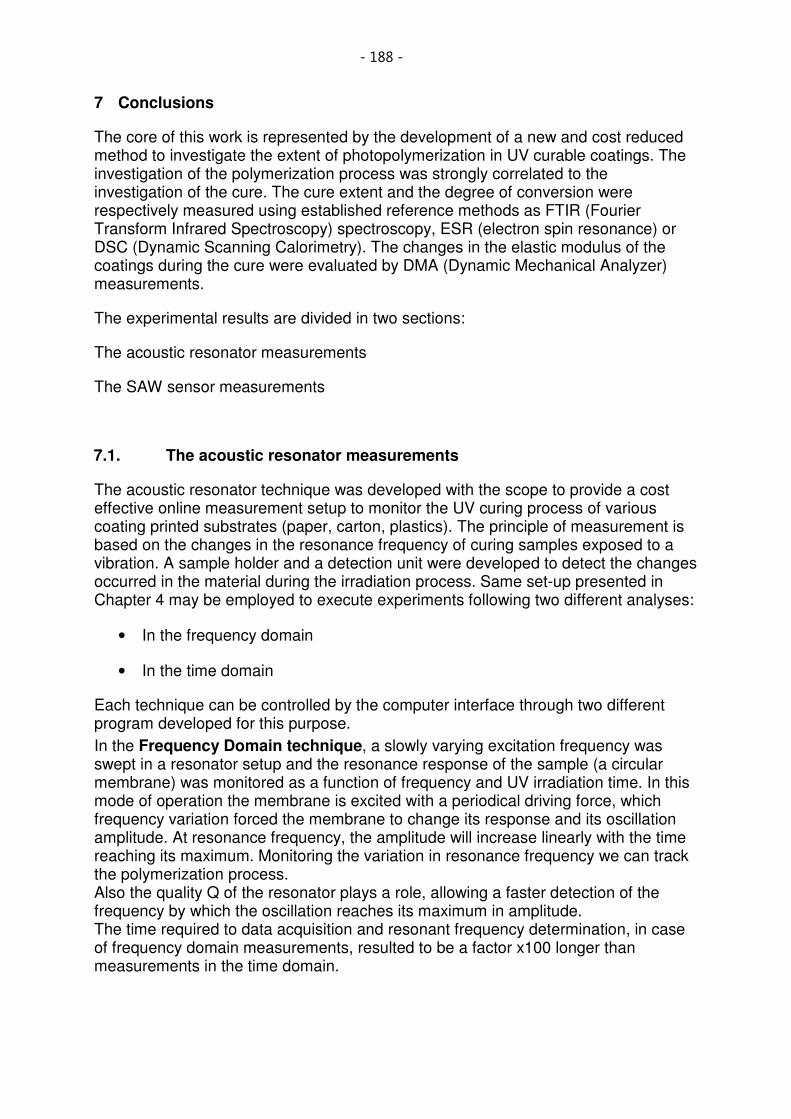
- 188 -

7 Conclusions

The core of this work is represented by the development of a new and cost reduced method to investigate the extent of photopolymerization in UV curable coatings. The investigation of the polymerization process was strongly correlated to the investigation of the cure. The cure extent and the degree of conversion were respectively measured using established reference methods as FTIR (Fourier Transform Infrared Spectroscopy) spectroscopy, ESR (electron spin resonance) or DSC (Dynamic Scanning Calorimetry). The changes in the elastic modulus of the coatings during the cure were evaluated by DMA (Dynamic Mechanical Analyzer) measurements.

The experimental results are divided in two sections:

The acoustic resonator measurements

The SAW sensor measurements

7.1. The acoustic resonator measurements

The acoustic resonator technique was developed with the scope to provide a cost effective online measurement setup to monitor the UV curing process of various coating printed substrates (paper, carton, plastics). The principle of measurement is based on the changes in the resonance frequency of curing samples exposed to a vibration. A sample holder and a detection unit were developed to detect the changes occurred in the material during the irradiation process. Same set-up presented in Chapter 4 may be employed to execute experiments following two different analyses:

• In the frequency domain

• In the time domain

Each technique can be controlled by the computer interface through two different program developed for this purpose.

In the Frequency Domain technique, a slowly varying excitation frequency was swept in a resonator setup and the resonance response of the sample (a circular membrane) was monitored as a function of frequency and UV irradiation time. In this mode of operation the membrane is excited with a periodical driving force, which frequency variation forced the membrane to change its response and its oscillation amplitude. At resonance frequency, the amplitude will increase linearly with the time reaching its maximum. Monitoring the variation in resonance frequency we can track the polymerization process. Also the quality Q of the resonator plays a role, allowing a faster detection of the frequency by which the oscillation reaches its maximum in amplitude. The time required to data acquisition and resonant frequency determination, in case of frequency domain measurements, resulted to be a factor x100 longer than measurements in the time domain.

- 189 -

In Time Domain technique, the membrane was excited by a short and intense, rectangular pulse, and its oscillation and slow decay was monitored by the detection unit as function of frequency and irradiation time. In this operation mode, after excitation the membrane continues to oscillate on its resonance frequency for a while until attenuation occurred.

For a given quality Q of the resonator, we can expect Q free oscillations before the oscillation amplitude has decayed to 1/e of its original amplitude. If Q is high enough, we can thus easily determine the eigenfrequency and the attenuation factor of the oscillator, responding to a short excitation. Once the free oscillation has ceased, a new pulse can be sent towards the membrane to excite another free oscillation. This way, a series of delta pulses can repeatedly excite a series of free, attenuated oscillations for accurate signal processing.

The time domain technique allows a much faster measurement, about 10 ms with respect to the frequency domain technique, where a standard measurement takes about 2 min. Moreover, the time domain operation mode would also permit the monitoring the dynamic of the photopolymerization process.

Because of aging phenomenon occurred in the paper substrate during UV irradiation (see Chapter 4, Paragraph 4.7.2) we divided the results obtained in the frequency domain technique in two main parts, depending on the substrate used for the samples.

7.1.1. Paper substrate

The results obtained on paper samples showed an unexpected gradual decrease of the resonance frequency with the increase of the irradiation time for all the samples when prepared in labour conditions; unexpected though, when taking into account just the polymerisation process. The typical curve representing our experimental results exhibits three distinct regions (Fig.4.25,Chapter 4).

The first region referred to the first 20 to 30 minutes of irradiation and can be correlated to the start of cure. The resonance frequency (fres=1670 Hz) presented a gradually decrease in the range of 80 Hz with the increase of irradiation time. This decrease corresponds to a drop of approximate 200 MPa in the material storage modulus and an increase from 0.040 to 0.045 of the tanδ, measured by DMA (Dynamic Mechanical Analyzer) in Chapter 6.

The second region exhibited an abrupt decrease in the resonant frequency (fres=1645 Hz) in the range of 100 Hz for an irradiation time of approximate 15 minutes. This point showed as a “knee” in the frequency plot. The storage modulus showed a decrease of approximate 500 MPa. In the meantime the loss modulus registered an increase of 600 MPa and tanδ increase from 0.042 to 0.048.

The third region showed a saturation of the signal for an endless irradiation time and was related to the end of cure. The storage modulus, obtained by DMA measurements rested fixed at 2400 MPa and the tanδ registered a peak at 0.052. The new formed polymer network reached the vitrification point,which prohibited further reactions, although a very slow diffusion controlled reaction may be observed in the glassy state.

- 190 -

Table 7. 1: Decrease in the resonant frequencies with the cure progress for labour sample’s printed onto paper substrate The “knee” indicates the first transitions sensed after approximate 30 min of cure.

Responsible for the “unexpected” decrease in the resonant frequency with increase of the irradiation time, trend which opposites the theory, are two phenomena registered into the paper substrate. On the one hand, the paper substrate undergoes under intense UV irradiation chemical reactions, due to the collapse of double bonds in the adhesives used by paper manufacturing [25]. This collapse corresponds to a substantially decrease in the resonant frequency of the vibrating substrate. On the other hand, the UV irradiation generates the evaporation of the humidity accumulated in the paper during the storage, which automatically implies a mass loss in the investigated samples. The decrease in the resonant frequency emerged with increase of the irradiation time represents the consequence of those two phenomena on our vibrating system (substrate+coating). The decrease tends to overwhelm the small increase, which in line with the theory, is to be expected with increase of the irradiation time and with increase of the crosslinking process, respectively. The substantially decrease in the resonant frequency was, unfavourable exceeded by the long irradiation times required by our labour UV lamp with limited power. To confirm the above explanation, we investigated samples stored, printed and irradiated in MAN Roland premises, by the use of professional equipment. The results showed an increase of the resonant frequency by increasing UV doses. The change in the resonant frequency confirmed also its dependency on the printing velocity (see Chapter 4), since velocity influenced the irradiation doses absorbed by the sample.

Table 7. 2: Change in the resonant frequency of the coating with the cure progress for sample’s printed onto paper substrate using a MAN Roland printed machine.

Colour Frequency(Hz)

Uncured Frequency(Hz)

Cured Frequency(Hz)

“knee”

Yellow 1675 1480 1625

Magenta 1765 1544 1672

Black 1876 1724 1860

Cyan 1853 1601 1845

Formulation Frequency(Hz)


Cured

Clear Coating 2110 2116

- 191 -

Nevertheless,a lower printing velocity resulted in a better photoploymerization degree than higher velocity printed sheets, which can implies costs reduction by using the half of UV doses which was requested to complete the process. Here is to note the change in the line shape of the amplitude, which increases with the irradiation time, exhibiting a sharper peak, sign of a decrease in the damping. 7.1.2. Plastic substrates The hypothesis that ageing and the mass loss induced through UV irradiation are responsible for the decreasing trend in the resonant frequency, with increasing of crosslinking in the paper substrate, was further confirmed by the investigations made on plastics substrates. Considering that the literature revealed no particular changes into the plastics materials (PVC) under UV illumination and that our experiments asserted no mass loss occurred under irradiation, we investigated coatings printed onto this substrate type. The first observation was that the amplitude at the resonant frequency is by far less affected by the UV irradiation as in the paper substrate case, and it increases with the irradiation time. The second result, opposite to those recorded with paper substrate, was a very small increase in the resonant frequency with increase of the irradiation time.

Table 7. 3: Change in the resonant frequency of the coating with the cure progress for plastic substrates.

These results showed that for coatings printed onto substrates with no sensitivity toward the UV irradiation (chemical or mechanical), the resonant frequency registers an increase with the increase of the crosslinking process, induced through the irradiation. The change in the resonant frequency as well as the change in the line shape of the amplitude is due to the decrease in the damping, as consequence of the new polymer matrix formed. The thicknesses of the coating together with the irradiation time are two factors,which significantly affect the change in the resonant frequency. 7.1.3. Summary

The frequency domain method can identify the extent of polymerization process and through the changes in the resonant frequency plot can predict the main transitions in the dynamic of photopolymerization process. The main advantage of this method over most laboratory based analysis techniques is the set-up simplicity and the

Colour Frequency(Hz)


Cured

Cyan 1823 1825

- 192 -

promptness of results. Because it is based on acoustic wave propagation principle only small amount of material may be employed.

The time domain method provided the same results like the frequency domain method with less precision. The advantage of the time domain technique with respect to the frequency domain technique is the very fast measurement time and the possibility to monitor the dynamic of the polymerization process. This characteristic permits to measure in real time and record all transitions occurred in the photopolymerization process.

Both techniques may be controlled over computer interface using adequate software programs developed for the purpose.

The developed techniques fulfil the request of fast, cost reduced methods to investigate the extent of photopolymerisation. Furthermore, these techniques permit to detect the transitions,which were induced in the material by irradiation. These were detected like distinct regions in the frequency plot. The first transition, corresponding to the polymer network formation, appears like the onset in the frequency plot, while the saturation value of the resonant frequency marks the end of polymerisation

The set-up, controlled over the computer interface, was tested for all four coatings pigmentation. The results are repeatable with slight differences for each colour. T

In the time domain operation mode is required an optimization of the set-up to avoid the UV light penetration into the photodiode and to overshadow like that the measurement signal. Some simply procedures, like a protection screen for the photodiode or setting the irradiation on the front of the sample and the measurement unit on the rear side of the sample, can overcome this problem.

With such careful procedures,the time domain technique may be successfully applied in-line and help to maximise the productivity due to real time operation.

The frequency domain technique does not require particular care in the setup procedure. Nevertheless, this operation mode is more suitable for quality measurements and less for production control. This is due to its higher accuracy, but relative long measurement time, inadequate to very fast production printing machines.

In Chapter 4 are displayed the results obtained on products printed in the machine. The test encompassed 58 different products printed on different substrate and coated with different formulation. The obtained results are repeatable and displayed considering the UV lamp irradiation power (W/cm) and the printing velocity (B/h).

- 193 -

7.2. The SAW sensor measurements

Acoustic wave sensors are widely employed in the detection and measurements of different materials. They can sense various phenomenons’s and give information about the reactions and process occurred in those materials.

The SAW (surface acoustic wave) sensor is capable of sensing transition behaviours in the coatings applied as thin films to its surface. The changes in polymer properties at the glass transition temperature are detected as changes in the transmission plot. The transitions induced in the coatings samples through UV irradiation are sensed as an increase in the acoustic wave damping.

The acoustic loss, sensed as an increase in the damping of the acoustic wave, was of approximately 3-4 dB, depending of pigmentation, value obtained from the signal recorded at the uncured state and the cured state of the material.

Tabel 7. 2: The increase in the damping constant for three different pigmented coatings. The length of the sample along the saw path was 4 mm.

The measurements performed demonstrated that the application of a multilayer system composed of a coating formulation and a polymer substrate onto a SAW device, presented a strong impact on the transmission behaviour of the acoustic wave. The dependence of the SAW attenuation on the cure progress and therefore on the coatings transitions are reflected on the exponential decrease of the transmission. From the delay in the irradiation start time, the measurements recorded at turn-off the UV light and the scan of the frequencies spectra, the obtained results may be assigned to the changes in the mechanical properties of the coatings, induced during irradiation.

The clear coatings showed a strong impact on the sensor signal sensed as an increase in the amplitude of the acoustic wave with increase of the irradiation time. The difference between the start of irradiation and the value where the amplitude signal reached its saturation value was of 25 dB.

For each colour a statistic should be compiled where the damping factor depends on the length and the thickness of the sample in order to confirm the reproducibility of the measurements results.

Another issue consists in the SAW device itself. In the current set-up the coating film must be printed and cut to the right size before the application on the device and

Signal RedCured/Uncure

d

YellowCured/Uncured

CyanCured/Uncured

Clear Cured/Uncured

Transmission

[dB] -30/-33 -28/-31 -31/-35

∆~5 (calculated)

Damping constant

[dB/mm] 0,75 0,875 1 1,25

Thickness (µm) 1,35 1,65 1,65 2

- 194 -

furthermore the SAW device may be used for one measurement operation only. Here is the need of a method to recycle the SAW device and to permit the size adjustment directly on the printed products. A new cleaning agent or a protection coating for the SAW device, which would avoid the intimate contact between colour and SAW device, may represent a solution.

In conclusion, the approach with the SAW sensor seems not to be suitable for inline measurements in mass production equipment, where many variables could affect the high sensitivity of the measurements.

Appendix The software program used for the Frequency Domain Technique.

The test matrix used in the ManRoland printing test.

Härtungskontrolle 25.6.2010; PTC R506

Magdalena DeAmbroggi

Farbe printcom S201 V-UV

Lack printcom S701 U

Rasterwalze 18 cm³/m²

Feuchtmittel

printcom S130 X + 5 % IPA

Druckwerk 4-7

Substrat Lack Farbe Trocknerleistung Geschwindigkeit

41 Luxo Magic 150 g/m² x - 0 5000 B/h nass

44 Luxo Magic 150 g/m² x - UV-E: 1 x 160 W/cm 10000 B/h



45 Luxo Magic 150 g/m² - Magenta 0 5000 B/h nass

48 Luxo Magic 150 g/m² - Magenta UV-E: 1 x 160 W/cm 10000 B/h



1 MegaGloss 150 g/m² x - 0 5000 B/h nass

5 MegaGloss 150 g/m² - Magenta 0 5000 B/h nass

9 MegaGloss 150 g/m² x Magenta 0 5000 B/h nass

13 MegaGloss 150 g/m² - Magenta + Gelb 0 5000 B/h nass

17 MegaGloss 150 g/m² x Magenta + Gelb 0 5000 B/h nass

37 MegaGloss 150 g/m² - - (nur Feuchtmittel

DW7) 0 5000 B/h

40 MegaGloss 150 g/m² x Schwarz + Cyan +

Magenta 0 5000 B/h nass

4 MegaGloss 150 g/m² x - UV-E: 1 x 160 W/cm 10000 B/h

8 MegaGloss 150 g/m² - Magenta UV-E: 1 x 160 W/cm 10000 B/h

12 MegaGloss 150 g/m² x Magenta UV-E: 1 x 160 W/cm 10000 B/h

16 MegaGloss 150 g/m² - Magenta + Gelb UV-E: 1 x 160 W/cm 10000 B/h

20 MegaGloss 150 g/m² x Magenta + Gelb UV-E: 1 x 160 W/cm 10000 B/h

38 MegaGloss 150 g/m² - Magenta (trockene

Fläche) UV-E: 1 x 160 W/cm 10000 B/h






39 MegaGloss 150 g/m² x Schwarz + Cyan +

Magenta UV-E: 2 x 160 W/cm 10000 B/h






49 OptiGloss 150 g/m² - Magenta 0 5000 B/h nass

52 OptiGloss 150 g/m² - Magenta UV-E: 1 x 160 W/cm 10000 B/h



25 PVC - Magenta 0 5000 B/h nass

28 PVC - Magenta UV-E: 1 x 160 W/cm 10000 B/h



References

[1] S Pappas, Radiation Curing, Science and Technology, Plenum Press, New York(1992). [2] J Fouassier and J. F. Rabek (Fds), Radiation Curing in Polymer Science and Technology, Plenum Press, New York, 453, 1989. [3] Eichler, Herz, Naito, Schnabel, J Photochem,1980, 12, 225.

[4] H. J. Hageman, Progr. Org. Coat 13, 123,1985. [5] C. Decker and K. Moussa, J. Applic. Polym. Sci. 34, 1603 (1987). [6] J. P. Fouassier, J. Radiation Curing 17 (3), 9 (1990). [7] H.M.J. Boots, Integration of Fundamental Polymer Science and Technology,204, Elsevier Applied Science London, 1986. [8] S. P. Pappas, J. Radiation Curing 14 (3), 6 (1987). [9] J. G. Kloosterboer and G. M. Lippits, J. Radial. Curing 11 (l), 1 (1984). [10] L. Lessinger, Morse Oscillators, Birge Sponer Extrapolation, and the Electronic Absorption-Spectrum of I2, Journal of Chemical Education, 71, 388-391,1994. [11] P. C. Schmidt, K. G. Weil, Atom- und Molekülbau, Georg Thieme Verlag, Stuttgart - New York, 1982. [12] P. W. Atkins, Physikalische Chemie, Vol. 3, Wiley-VCH, 2001. [13] C. Decker, Light-induced crosslinking polymerization, Polymer International, 51, 1001-1150, 2002. [14] C. Decker, Macromolecules 23,5217 (1990). [15] Michaud, V.; Manson, J.A.E. · Mar 1, 2006. [16] H.C. Van der Hulst, Light scattering by small particles. Dover Publ., New York, Dover, 1981 [17] G. Jeschke, H. W. Spieß, Skript - Einführung in die ESR-Spektroskopie, 1998. R. Brückner, Reaktionsmechanismen, Vol. 3, Spektrum Akademischer Verlag, 2004. [18] Schneider, E. E. , Day, M. J. , and Stein, G. , Nature, 168, 645 (1951). [19] RS Bradley , Atomic force microscope. Phys. Rev. Lett., 56:930-933, 1986 [20] D. Drechsler, A. Karbach and H. Fuchs. Nanoindentation on polycarbonate/ polymethyl methacrylate Blends. Appl. Phys. A 66, 825–829, 1998. [21] Dr E Cockburn & Dr R Holman, The Effects of Volume Changes during Polymerisation for Some Radcure Coatings, 1992. [22] L. E. Kinsler, A.R. Frey, A. B. Coppens and J.V. Sanders,' Fundamentals of Acoustics', John Wiley,95,99,102, 1982 [23] Karrenberg,U. „Signale Prozesse Systeme. Eine multimediale und interaktive Einführung in die Signalverarbeitung“,Springer Verlag Berlin Heidelberg New York 2000 (2003) [24] Schnorrenberg, W.: Spektrumanalyse Theorie und Praxis. Verlag Vogel Würzburg 1990. [25] Izdebska J., Baranowska A., and Podsialdl H., [26] Neubig, B., Briese, W.: Das große. Quarzkochbuch; Franzis-Verlag GmbH. (1997) [27] Mauder Anton. SAWGas Sensors: Comparison between Delay-line and Two-PortResonator. Sensors and Actuators B, Band 26, (1995), 187–190 [28] L. Spassov, Sens.Actuators A: Phys. 30 (1992), 67–72

[29] H. Ziegler, A low-cost digital sensor system, Sensors and Actuators, 5 (1984) 169-178. [30] J. Campbell, Surface Acoustic Wave Devices and Their Signal Processing Application, Academic Press Inc., Boston, (1989).

[31] R. Peach, On the existence of surface acoustic waves on piezoelectric substrates, IEEE Trans. Ultrason. Ferroel. Frequ. Contr., 48 (2001) 1308-1320. [32] G. Sauerbrey, Verwendung von Schwingquarzen zur Wägung dünner Schichten und zur Mikrowägung, Z. Phys., 155 (1959) 206-222. [33] C. Lu and A.W. Czanderna, Eds., Applications of Piezo electric Quartz Crystal Microbalances (Elsevier, Amsterdam, 1984). [34] K.K. Kanazawa, J.G. Gordon II, The Oscillation Frequency of a Quartz Resonator in Contact with a Liquid, Anal. Chim. Acta, 175 (1985) 99-105. [35] L.J.W.S. Rayleigh, On waves propagated along the plane surface of an elastic solid, Proceedings of the London Mathematical Society, 17, 4 (1885) [36] M. Rapp, Chemische Sensorik mit akustischen Oberflächenwellen, Dissertation, Universität Heidelberg, (1991). [37] F.A. Firestone, J.A. Frederick, J. Acoust. Soc. Amer., 18 (1946) 200-211. [38] R.M. White, F.W. Voltmer, Appl. Phys. Lett., 7 (1965) 314-316. [39] Auld B. A. Acoustic Fiels and Waves in Solids, Band 2. Robert E. Krieger Publishing, Malabar, Florida, 2. Auflage, 1990 [40] Stone David C. und Thompson Michael. Interdigital Capacitance and Surface Acoustic Wave Sensors. Analytical Chemistry, Band 65, 1993, 352–362

[41] K.K. Wong, Properties of Lithium Niobate, EMIS Data reviews Series No. 28, 1989 [42] S.J. Martin, G.C. Frye, S.D. Senturia, Dynamics and response of polymer-coated surface acoustic wave devices: Effect of viscoelastic properties and film resonance, Anal. Chem., 66 (1994) 2201-2219. [43] Weigel R. Akustische Oberflächenwellen-Bauelemente im UHF-Bereich. VDI Fortschittsberichte,VDI Verlag, 1993 [44] S.J. Martin, G.C. Frye, A.J. Ricco, T.E. Zipperian, Proc. IEEE Ultrason. Symp., (1987) 563-567. [45] Datta,Surface Acoustic Wave Devices, Prentice-Hall, 1986 [46] A. Ballato. 1996. “Piezoelectricity: History and New Thrusts,” Proc Ultrasonics Symposium, Vol. 1:575-583. [47] K. Bodenhöfer, A. Hierlemann, G. Noetzel, W. Göpel, Performance of Mass-Sensitive Devices for Gas Sensing: Thickness Shear Mode and Surface Acoustic Wave Transducers, Anal. Chem., 68 (1996) 2110-2118.

[48] H. Wohltjen and R. Dessy. 1979. “Surface Acoustic Wave Probe for Chemical Analysis I. Introduction and Instrument Design,” Ana Chem, Vol. 51 (9):1458-1475. [49] R. Lucklum, C. Behling, P. Hauptmann, Role of Mass Accumulation and Viscoelstic Film Properties for the Response of Acoustic-Wave-Based Chemical Sensors, Anal. Chem., 71 (1999) 2488-2496.

[50] R. Lucklum, C. Behling, P. Hauptmann, Signal amplifiction with multilayer arrangements on chemical quartz-crystal-resonator sensors, IEEE Trans. Ultrason. Ferroel, Frequ. Contr., 47 (2000) 1246-1252. [51] Butler M. A. et al. Gas Sensing with Acoustic Devices. In: 1996 Ultrasonics Symposium. 1996, 423–434 [52] Frye G. C. und Martin S. J. Dynamics and Response of Polymer-Coated SurfaceAcoustic Wave Devices: Effect of Viscoelastic Properties and Film Resonance.Analytical Chemistry, Vol. 66 [53] Barnes J. A. et al. Characterization of Frequency Stability. IEEE Transactions on Instrumentation and Measurement , Band 20, Nr. 2, 1971, 105–120

[54] J. Grate, S. Martin, and R. White. 1993. “Acoustic Wave Microsensors,” Analytical Chemistry, Vol. 65, No. 21:940-948.

[55] H. Wohltjen. 1987. op. cit. [56] Hartmann B. Acoustic Properties. In: Encyclopaedia of Polymer Science and Engineering, John Wiley & Sons, Inc., New York, Band 1. 1984, 131–160 [57] H. Wohltjen and R. Dessy. 1979. “Surface Acoustic Wave Probe for Chemical Analysis I. Introduction and Instrument Design,” Ana Chem, Vol. 51 (9):1458-1475. [58] Gillham, J. K. and Roller, M. B. (1971) Polym. Eng. Sci. 11 , 295

[59] Haran , E. N. , Gringras, H. and Katz, D. (1965) J. Appl. Polym. Sci. 9 , 3505

[60] R.T. Smith, F.S. Welsh, Temperature dependence of the Elastic,Piezoelectric, and Dielectric Constants of Lithium Tantalate and Lithium Niobate, (1971).

[61] Landau L. D. und Lifschitz E. M. Lehrbuch der theoretischen Physik, Band 7. Akademie-Verlag, Berlin, 1970 [62] Ferrry,J.D., Viscoelastic Properties of Polymers, John Wiley & Sons, Inc. , New York,London (1961) [63] Kloosterboer, J.G., G.M.M. van der Hei, R.G. Gossink, Dortnat, GCM, „Polymer Communications“, 1994,25,322. [64] Anseth, K.S., Bowman,C.N.,Pepass,N.A., „J.Polym.Sci“ Part A, Polym Chem,1994,32,139. [65] Skelhorne, G.G.,“Chemistry and Technology of UV and EB Formulations for Coatings, Inks and Paints“, Vol.1 ed. P.K.T. Oldring, SITA Technology Ltd. London, 1991, 101-157. [66] Nablo, S.V., “Radiation Curing in Polymer Science & Technology”, Vol.1, eds. JP Fouasssier and JF Rabek, Elsevier Applied Science London UK, 1993,503.

[67] Davidson, R.S., “For a discussion of the effects of oxygen upon radical initiated polymerisation reactions”, “Polymer Science and Technology”, Vol.III, Elsevier Applied Science London UK, 1993,153.

[68] Davidson, R., “Molecular Association”, Vol.I, Academic Press, London UK,1975,215. [75] Fischer, H.,Baer,R.,Verhoolen,R.Hany,Walbinder,M.,“J Chem Soc“ Perkin Trans 2, 1990,787. [76] B. Carlowitz. Kunststoff–Tabellen. 3. Aufl. (Carl Hanser Verlag München, Wien), 1986. [77] Hoyle, C.H., „Radiation Curing of Polymeric Materials“, Am Chem Soc Symp,1990, 417-420. [78] K. Studer et al. / Progress in Organic Coatings 48 (2003) 101–111.

[79] Hörner, A., Untersuchungen von Metall-Isolator-Übergängen mit Oberflächenwellen, opus.bibliothek-uni-augsburg.de [80] H. Matthews, Surface Wave Filters, Wiley-Interscience publication,197 [81] http://www.bostonpiezooptics.com [82] Jun-ichi Kushibiki et al., ieee transactions on ultrasonics, ferroelectrics, and frequency control, vol. 46, no. 5, Sept. 1999 [83] Suppan,P., “Chemistry and Light”, Royal Society of Chemistry, Cambridge UK, 1994. [84] A.Gilbert and J. Baggott, “Essentials of Molecular Photochemistry”, Blackwell London, UK,1991. [85] www.chemgapedia.com [86] S.Thimoshenko, S. Wionowsky-Krieger, “Theory of Plates and Shells”, McGraw-Hill Book Company, 2 ed., 1959. [87] http://hyperphysics.phy-astr.gsu.edu. [88] Harris, Fredric J., “Multi-rate Signal Processing for Communication Systems”, Prentice Hall,May 24, 2004. [89] G. Wedler, Lehrbuch der Physikalischen Chemie, Vol. 5, Wiley-VCH, 2004.

[90] Marti, O. Instrumentation for scanning force microscopy and friction force mi-croscopy. In Micro/Nanotribology and Its Applications (Dordrecht), Vol. 330;Bhushan, B.,Ed.; Kluwer Academic Publishers: 1997. [91] Scherzer, Tom, Real-time FTIR-ATR spectroscopy of photopolymerization reactions, Macromolecular Symposia, Special Issue: Polymer Spectroscopy, Vol. 184, 79-98. [92] Hardinger, Steven H., The Chemical Educator, Vol. 3, Issue 3, 1998 Springer Verlag, N.Y.,Inc. [93] www.chemgapedia.de [94] TA Instruments, “User’s Book”., [95] Winter, Henning H., Chambon,F., Analysis of a Crosslinking Polymer at the Gel Point, Polym. Bull., 16, 499, 1986.

[96] X. Ramis, J. M. Salla, J. Polym. Sci. Part B: Polym. Phys. 35, 371 (1997)

[97] Rieger,J., The glass transition temperature of polystyrene, J. of Thermal Analysis and Calorimetry, Vol. 46, Nr. 3-4, 965-972.

[98] www.hyperphysics.edu

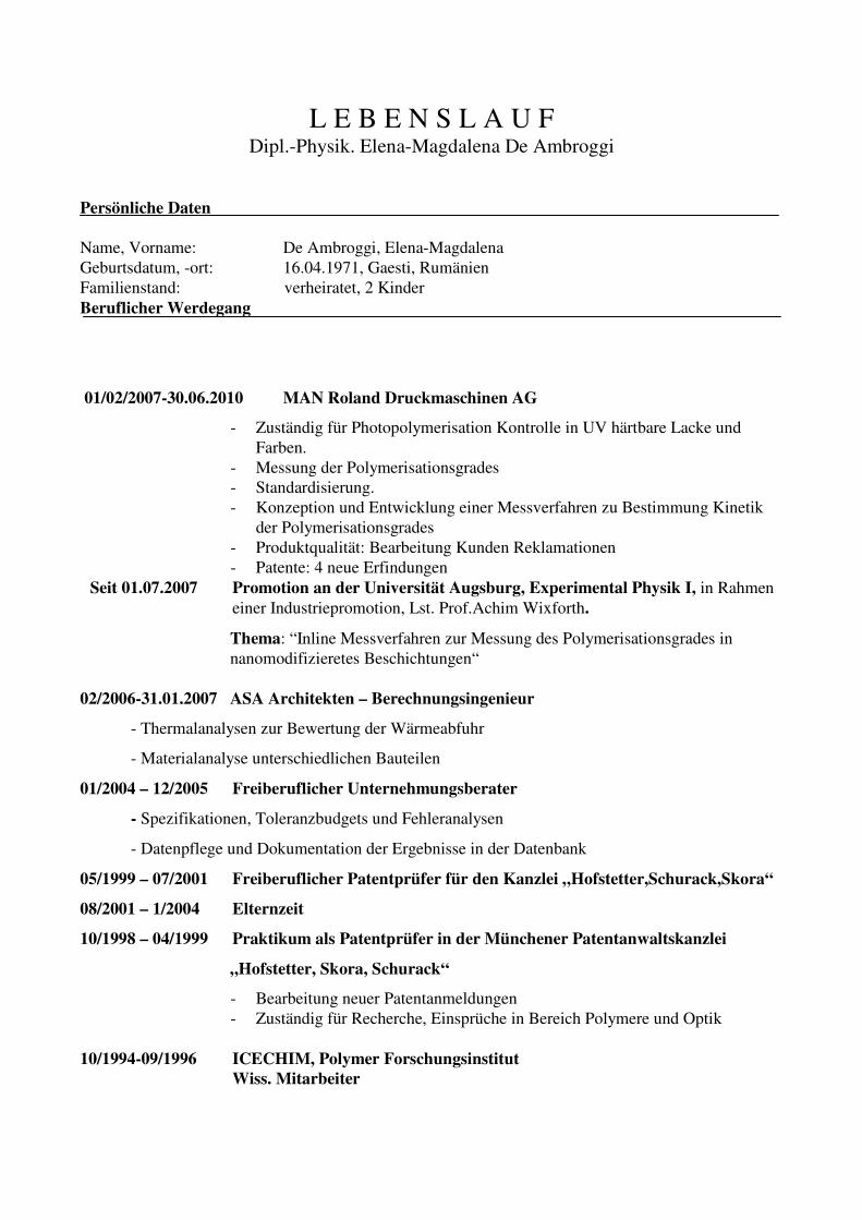
L E B E N S L A U F Dipl.-Physik. Elena-Magdalena De Ambroggi

Persönliche Daten

Name, Vorname: De Ambroggi, Elena-Magdalena

Geburtsdatum, -ort: 16.04.1971, Gaesti, Rumänien

Familienstand: verheiratet, 2 Kinder

Beruflicher Werdegang

01/02/2007-30.06.2010 MAN Roland Druckmaschinen AG

- Zuständig für Photopolymerisation Kontrolle in UV härtbare Lacke und

Farben.

- Messung der Polymerisationsgrades

- Standardisierung.

- Konzeption und Entwicklung einer Messverfahren zu Bestimmung Kinetik

der Polymerisationsgrades

- Produktqualität: Bearbeitung Kunden Reklamationen

- Patente: 4 neue Erfindungen

Seit 01.07.2007 Promotion an der Universität Augsburg, Experimental Physik I, in Rahmen

einer Industriepromotion, Lst. Prof.Achim Wixforth.

Thema: “Inline Messverfahren zur Messung des Polymerisationsgrades in

nanomodifizieretes Beschichtungen“

02/2006-31.01.2007 ASA Architekten – Berechnungsingenieur

- Thermalanalysen zur Bewertung der Wärmeabfuhr

- Materialanalyse unterschiedlichen Bauteilen

01/2004 – 12/2005 Freiberuflicher Unternehmungsberater

- Spezifikationen, Toleranzbudgets und Fehleranalysen

- Datenpflege und Dokumentation der Ergebnisse in der Datenbank

05/1999 – 07/2001 Freiberuflicher Patentprüfer für den Kanzlei „Hofstetter,Schurack,Skora“

08/2001 – 1/2004 Elternzeit

10/1998 – 04/1999 Praktikum als Patentprüfer in der Münchener Patentanwaltskanzlei

„Hofstetter, Skora, Schurack“

- Bearbeitung neuer Patentanmeldungen

- Zuständig für Recherche, Einsprüche in Bereich Polymere und Optik

10/1994-09/1996 ICECHIM, Polymer Forschungsinstitut

Wiss. Mitarbeiter

.

10/1996 – 09/1998 Gymnasium “V.Streinu”

Physik Unterricht

Ausbildung

Universität

10/1989-08/1994 Diplom als Physikerin:

10/10 Punkten beim Diplom, Universität von Bukarest, Physik Fakultät

Thema der Abschlussarbeit:„Physikalische Eigenschaften der flüssige Kristalle“

Schule

09/1985-08/1989 Wissenschaftliches Gymnasium „Vladimir Streinu“, Rumänien

Abschluss Wissenschaftliche Hochschulreife

Sonstige Kenntnisse/ Erfahrungen

Sprachen:

- Rumänisch: Muttersprache

- Deutsch: Verhandlungssicher

- Italienisch: Muttersprache

- Englisch: Verhandlungssicher

- Französisch: Sehr gut

Documents

Acoustic monitoring of photopolymerization in UV curable coatings · 2016-05-18 · Acoustic monitoring of photopolymerization in UV curable coatings Dissertation zur Erlangung des