arX

iv:c

ond-

mat

/990

9315

v1 2

1 Se

p 19

99

Acoustic Energy and Momentum in a Moving Medium

MICHAEL STONE

University of Illinois, Department of Physics

1110 W. Green St.

Urbana, IL 61801 USA

E-mail: m-stone5@uiuc.edu

Abstract

By exploiting the mathematical analogy between the propagation of sound

in a non-homogeneous potential flow and the propagation of a scalar field in a

background gravitational field, various wave “energy” and wave “momentum”

conservation laws are established in a systematic manner. In particular the

acoustic energy conservation law due to Blokhintsev appears as the result of

the conservation of a mixed co- and contravariant energy-momentum tensor,

while the exchange of relative energy between the wave and the mean flow

mediated by the radiation stress tensor, first noted by Longuet-Higgins and

Stewart in the context of ocean waves, appears as the covariant conservation

of the doubly contravariant form of the same energy-momentum tensor.

PACS numbers: 43.28.Py, 43.20.Wd, 43.25.Qp, 67.40.Mj

Typeset using REVTEX

1

I. INTRODUCTION

Many discussions of the “energy” and “momentum” associated with waves propagating

through moving fluids can be found in the physics [1], engineering [2–6], and mathematical

fluid mechanics literature [7–16]. Various definitions are proposed, some of which lead to

conserved quantities, and some to quantities that are not conserved but instead exchanged

between the wave and the mean flow. In part the multiplicity of definitions is due to difficulty

in deciding what fraction of the energy or momentum of the system properly belongs to the

wave and what fraction should be associated with the moving medium. It is also often

unclear how to divide equations expressing conservation laws into terms relating to the

conserved quantity, and terms acting as sources for this quantity. Related to these primarily

cosmetic problems are more fundamental issues as to whether the “energy” or “momentum”

under discussion is the true newtonian energy or momentum, or instead pseudo-energy and

pseudomomentum. Thus we have the question “what is the momentum of a sound wave”

raised by Sir Rudolf Peierls in his book Surprises in Theoretical Physics [17], and the salutary

polemic “On the ‘Wave Momentum’ Myth” by M. E. McIntyre [18].

The most extensive analyses of conserved wave properties have been carried out by the

fluid mechanics community [7–15]. Typically these papers adopt a lagrangian (following

individual particles in the flow) or mixed lagrangian-eulerian approach, as opposed to the

purely eulerian (describing the flow in terms of a velocity field) approach which would be

most familiar to a physicist. In addition a physicist reading this literature feels the lack of

a general organising principle behind the definition and derivation of the conservation laws.

The present paper is intended to remedy some of these problems — at least for the special

case of sound waves propagating through an irrotational homentropic flow. Although rather

a restricted class of motions, this is still one of considerable interest in condensed matter

physics. It includes phonon propagation in a bose condensate, and therefore lies at the heart

of the two fluid model of superfluids. By exploiting W. Unruh’s ingenious identification

[19,20] of the wave equation for sound waves in such a flow with the equation for a scalar

2

field propagating in a background gravitational field, I extract the conservation laws from

the principle of general covariance. Deriving the conservation laws in this way may seem

like a case of taking a sledge-hammer to crack a nut, but the formalism is familar to most

physicists, automatic in application, and the ambiguities in defining the conserved quantities

turn out to lie in the choice of whether to identify the energy-momentum tensor as T µν or as

T µν . Also, when quantities are not conserved, as is the case of the wave momentum in a shear

flow, their sources arise naturally from the connection terms in the covariant derivative.

In section two I discuss the action describing the irrotational motion of an homentropic

fluid. In section three I derive Unruh’s equation from the action principle. In section four I

explain why we often need information beyond the solutions of linearized wave equation, and

in section five derive the conservation equations that follow from the linearized equation.

Section six interprets these equations in terms of the motion of phonons. The discussion

section repeats the warnings from [18] that the appearance of quantum quasi-particles in any

argument is a sure sign that the we are considering pseudomomentum and not the actual

momentum of the system.

The work reported here was motivated by a desire to understand better the role of

acoustic radiation stress in the two-fluid model of a superfluid. It may be relevent to the

recent controversy [22–24] over the Iordanskii force acting on a vortex moving with respect to

the normal fluid component. The use of the Unruh formalism in this context was suggested

by Volovik [25].

II. THE ACTION PRICIPLE

The most straight forward way of deriving conservation laws starts from an action prin-

ciple. Noether’s theorem then provides us with an explicit formula for a conserved quantity

corresponding to each symmetry of the action. In fluid mechanics, unfortunately, at least

when we restrict ourselves to an eulerian decription of the flow field, action principles are

in short supply. Of course there must exist some action principle because ultimately the

3

fluid can be treated as a system of particles. A particle-based action, however, requires a

lagrangian description of the flow. When it is re-expressed in eulerian terms constraints

appear, and these limit its utility.

If we restrict ourselves to flows that are both irrotational and homentropic — the latter

term meaning in practice that we assume the pressure to be a function of the fluid density

only — then the number of degrees of freedom available to the fluid is dramatically reduced.

In this case the eulerian equations of motion are derivable from the action [26]

S =∫

d4x{

ρφ +1

2ρ(∇φ)2 + u(ρ)

}

. (2.1)

Here ρ is the mass density, φ the velocity potential, and the overdot denotes differentiation

with respect to time. The function u may be identified with the internal energy density.

Equating to zero the variation of S with respect to φ yields the continuity equation

ρ+∇ · (ρv) = 0, (2.2)

where v ≡ ∇φ. Varying ρ gives Bernoulli’s equation

φ+1

2v2 + µ(ρ) = 0, (2.3)

where µ(ρ) = du/dρ. In most applications µ would be identified with the specific enthalpy.

For a superfluid condensate the entropy density, s, is identically zero and µ is the local

chemical potential.

It is worth noting that our action could not have arisen from some rewriting of the

action for the motion of a system of individual particles. We are allowing variations of ρ

without requiring simultaneous variations of φ, and such variations conjure new matter out

of nothing.

The gradient of the Bernoulli equation is Euler’s equation of motion for the fluid. Com-

bining this with the continuity equation yields a momentum conservation law

∂t(ρvi) + ∂j(ρvjvi) + ρ∂iµ = 0. (2.4)

4

We simplify (2.4) by introducing the pressure, P , which is related to µ by P (ρ) =∫

ρdµ.

Then we can write

∂t(ρvi) + ∂jΠji = 0, (2.5)

where Πij is given by

Πij = ρvivj + δijP. (2.6)

This is the usual form of the momentum flux tensor in fluid mechanics.

The relations µ = du/dρ and ρ = dP/dµ show that P and u are related by a Legendre

transformation, P = ρµ − u(ρ). From this and the Bernoulli equation we see that the

pressure is equal to minus the action density,

− P = ρφ+1

2ρ(∇φ)2 + u(ρ). (2.7)

Consequently we can write

Πij = ρ∂iφ∂jφ− δij

{

ρφ+1

2ρ(∇φ)2 + u(ρ)

}

. (2.8)

This is the flux tensor that would appear were we to use Noether’s theorem to derive a law

of momentum conservation directly from the invariance of the action under the translation

φ(r) → φ(r−a), ρ(r) → ρ(r−a). This is not a trivial point because there are at two similar,

but distinct, notions of “momentum”. True momentum is associated with the symmetry of

the action under a simultaneous translation all the particles in the system. Its conservation

requires an absence of external forces. Pseudomomentum [21] is the quantity that is pre-

served when the action is left invariant when the disturbance in the medium is relocated,

but the reference position of each individual particle is left unchanged. Conservation of

pseudomomentum requires homogeneity of the medium rather than of space. Replacing the

field φ(r) by φ(r − a) would normally correspond to the latter symmetry, but, because of

the absence of explicit particles, at this point in our discussion the two concepts coincide.

5

III. THE UNRUH METRIC

We now obtain the linearized wave equation for the propagation of sound waves in a

background mean flow. Let

φ = φ(0) + φ(1)

ρ = ρ(0) + ρ(1). (3.1)

Here φ(0) and ρ(0) define the mean flow. We assume that they obey the equations of mo-

tion. The quantities φ(1) and ρ(1) represent small amplitude perturbations. Expanding S to

quadratic order in these perturbations gives

S = S0 +∫

d4x

{

ρ(1)φ(1) +1

2

(

c2

ρ(0)

)

ρ2(1) +1

2ρ(0)(∇φ(1))

2 + ρ(1)v · ∇φ(1)

}

. (3.2)

Here v ≡ v(0) = ∇φ(0). The speed of sound, c, is defined by

c2

ρ(0)=

dµ

dρ

∣

∣

∣

∣

∣

ρ(0)

, (3.3)

or more familiarly

c2 =dP

dρ. (3.4)

The terms linear in the perturbations vanish because of our assumption that the zeroth-order

variables obey the equation of motion.

The equation of motion for ρ(1) derived from (3.2) is

ρ(1) = −ρ(0)c2

{φ(1) + v · ∇φ(1)}. (3.5)

In general we are not allowed to substitute a consequence of an equation of motion back

into the action integral. Here however, because ρ(1) occurs quadratically, we may use (3.5)

to eliminate it and obtain an effective action for the potential φ(1) only

S(2) =∫

d4x{

1

2ρ(0)(∇φ(1))

2 − ρ(0)2c2

(φ(1) + v · ∇φ(1))2}

. (3.6)

The resultant equation of motion for φ(1) is [19,20]

6

(

∂

∂t+∇ · v

)

ρ(0)c2

(

∂

∂t+ v · ∇

)

φ(1) = ∇(ρ(0)∇φ(1)). (3.7)

Note that in deriving this equation we have not assumed that the background flow v is

steady, only that it satisfies the equations of motion. Naturally, in order for our waves to

be distinguishable from the background flow, the latter should be slowly changing and have

a longer length scale than the wave motion.

Now (3.7) is equivalent to a perhaps more familiar equation [1]

(

∂

∂t+ v · ∇

)

1

c2

(

∂

∂t+ v · ∇

)

φ(1) =1

ρ(0)∇(ρ(0)∇φ(1)), (3.8)

as can be seen by using the mass conservation equation ∂tρ(0) +∇ · ρ(0)v = 0, but the form

(3.7) has the advantage that it can be written as1

1√−g∂µ√−ggµν∂νφ(1) = 0, (3.9)

where

√−ggµν =ρ(0)c2

1, vT

v, vvT − c21

. (3.10)

This is perhaps most easily seen by observing that the action (3.6) is equal to −S where

S =∫

d4x1

2

√−ggµν∂µφ(1)∂νφ(1) =∫

d4x√−gL. (3.11)

Equation (3.9) has the same form as that of a scalar wave propagating in a gravitational

field with Riemann metric gµν . The idea of writing the acoustic wave equation in this way,

as well as the general relativity analogy, is due to Unruh [19,20]. I will therefore refer to gµν

as the Unruh metric.

The 4-volume measure√−g is equal to ρ2(0)/c, and the covariant components of the

metric are

1I use the convention that greek letters run over four space-time indices 0, 1, 2, 3 with 0 ≡ t, while

roman indices refer to the three space components.

7

gµν =ρ(0)c

c2 − v2, vT

v, −1

. (3.12)

The associated space-time interval is therefore

ds2 =ρ(0)c

{

c2dt2 − δij(dxi − vidt)(dxj − vjdt)

}

. (3.13)

Metrics of this form, although without the overall conformal factor ρ(0)/c, appear in the

Arnowitt-Deser-Misner (ADM) formalism of general relativity [27]. There c and −vi are

refered to as the lapse function and shift vector repectively. They serve to glue successive

three-dimensional time slices together to form a four dimensional space-time [28]. In our

present case, provided ρ(0)/c can be regarded as a constant, each 3-space is ordinary flat R3

equipped with the rectangular cartesian metric g(space)ij = δij — but the resultant space-time

is in general curved, the curvature depending on the degree of inhomogeneity of the mean

flow v.

In the geometric acoustics limit sound will travel along the null geodesics defined by gµν .

Even in the presence of spatially varying ρ(0) we would expect the ray paths to depend only

on the local values of c and v, so it is perhaps a bit surprising to see the density entering

the expression for the Unruh metric. However an overall conformal factor does not affect

null geodesics, and thus variations in ρ(0) do not influence the ray tracing. For steady flow,

and in the case that only v is varying, it is shown in the appendix that the null geodesics

coincide with the ray paths obtained by applying Hamilton’s equations for rays

xi =∂ω

∂ki, ki = − ∂ω

∂xi, (3.14)

to the appropriate Doppler shifted frequency

ω(x,k) = c|k|+ v · k. (3.15)

When v is in the x direction only, we can also rewrite ds2 as

ds2 =ρ(0)c

{

− (dx− (v + c)dt) (dx− (v − c)dt)− dy2 − dz2}

. (3.16)

This shows that the x− t plane null geodesics coincide with the expected characteristics of

the wave equation in the background flow.

8

IV. MOMENTUM FLUX

The fluid in a sound wave has average velocity zero, but since the fluid is compressed

in the half cycle when it is moving in the direction of propagation and rarefied when it is

moving backwards there is a net mass current (and hence a momentum density) which is

of second order in the sound wave amplitude a0. This becomes clearer if one solves the

equation

dx

dt= v(x) = a0 cos(kx− ωt) (4.1)

for the trajectory x(t) of a fluid particle. This equation is non-linear (x appears inside the

cosine), and solving perturbatively one finds a secular drift at second order in a0.

x(t) = x(0) + oscillations +1

2a20

(

k

ω

)

t+ · · · . (4.2)

Although the time average of the eulerian fluid velocity, v, is zero, the time average of the

lagrangian velocity, vL = x, is not. The difference beweeen the two average velocities is the

Stokes drift . The Stokes drift is O(a20) while the wave equation is accurate only to O(a0), so

care is necessary before using its solutions to evaluate the mass current. Similar problems

occur in defining the energy density and energy and momentum fluxes which also require

second order accuracy.

We can expand the velocity field as

v = v + v(1) + v(2) + · · · , (4.3)

where the second-order correction v(2) arises as as consequence of the nonlinearities in the

equations of motion. This correction will possess both oscillating and steady components.

The oscillatory components arise because a strictly harmonic wave with frequency ω0 will

gradually develop higher frequency components due to the progressive distortion of the wave

as it propagates. (A plane wave eventually degenerates into a sequence of shocks.). These

distortions are usually not significant in considerations of energy and momentum balance.

9

The steady terms, however, represent O(a20) alterations to the mean flow caused by the sound

waves, and these often possess energy and momentum comparable to that of the sound field.

Even if we temporarily ignore these effects and retain only v(1) as determined from the

linearized wave equation, the density and pressure will still have expansions

ρ = ρ(0) + ρ(1) + ρ(2) + · · ·

P = P(0) + P(1) + P(2) + · · · . (4.4)

As before, the grading (n) refers to the number of powers of the sound wave amplitude in an

expression. The small parameter in these expansions is the Mach number given by a typical

value of v(1) divided by the local speed of sound.

Consider for example the momentum density ρv and the momentum flux

Πij = ρvivj + δijP. (4.5)

It is reasonable to define the momentum density and the momentum flux tensor associated

with the sound field as the second order terms

j(phonon) = 〈ρv〉 = 〈ρ(1)v(1)〉+ v〈ρ(2)〉, (4.6)

and

Π(phonon)ij = ρ(0)〈v(1)iv(1)j〉+ vi〈ρ(1)v(1)j〉+ vj〈ρ(1)v(1)i〉+ δij〈P(2)〉+ vivj〈ρ(2)〉. (4.7)

(The angular brackets indicate that we should take a time average over a sound wave period.

There is no need to consider terms first order in the amplitude because these average to zero.)

We see that to compute them we need to consider the second order contributions to both P

and ρ.

We can compute P(2) in terms of first order quantities from

∆P =dP

dµ∆µ+

1

2

d2P

dµ2(∆µ)2 +O((∆µ)3) (4.8)

and Bernoulli’s equation in the form

10

∆µ = −φ(1) −1

2(∇φ(1))

2 − v · ∇φ(1), (4.9)

together with

dP

dµ= ρ,

d2P

dµ2=

dρ

dµ=

ρ

c2. (4.10)

Expanding out and grouping terms of appropriate orders gives

P(1) = −ρ(0)(φ(1) + v · ∇φ(1)) = c2ρ(1), (4.11)

which we already knew, and

P(2) = −ρ(0)1

2(∇φ(1))

2 +1

2

ρ(0)c2

(φ(1) + v · ∇φ(1))2. (4.12)

We see that P(2) =√−gL where L is the Lagrangian density for our sound wave equation.

To extract ρ(2) in this manner we need more information about the equation of state

of the fluid than is used in the linearized theory. This information is most conveniently

parameterized by the logarithmic derivative of the speed of sound with pressure (a fluid-

state physics analogue of the Gruneisen parameter). Using this together with the previous

results for P(2), we find that

ρ(2) =1

c2P(2) −

1

ρ(0)ρ2(1)

d ln c

d ln ρ

∣

∣

∣

∣

∣

ρ(0)

. (4.13)

V. CONSERVATION LAWS

While we cannot compute the “true” energy and momentum densities and fluxes without

including non-linear corrections to the motion, it is often more useful find closely related

quantities whose conservation laws are a consequence of the linearized wave equation, and

which therefore provide information about the solutions of this equation. Our “general

relativistic” formalism provides a sytematic way of finding such conserved quantities. It is

well known [29] that any action S automatically provides us with a covariantly conserved

and symmetric energy-momentum tensor Tµν defined by

11

Tµν =2√−g

δS

δgµν. (5.1)

The functional derivative is here defined by

δS =∫

d4x√−g

δS

δgµνδgµν . (5.2)

It follows from the equations of motion derived from S that

DµTµν = 0, (5.3)

where Dµ is the covariant derivative. For example

DαAµν

σ = ∂αAµν

σ + ΓµαγA

γνσ + Γν

αγAµγ

σ − ΓγασA

µνγ. (5.4)

The Γαβγ are the components of the Levi-Civita connection compatable with the Unruh

metric, viz.

Γαβγ = gαρ[βγ, ρ], (5.5)

where

[βγ, ρ] =1

2

(

∂gγρ∂xβ

+∂gβρ∂xγ

− ∂gβγ∂xρ

)

. (5.6)

For our scalar field

T µν = ∂µφ(1)∂νφ(1) − gµν

(

1

2gαβ∂αφ(1)∂βφ(1)

)

. (5.7)

The derivatives with raised indices in (5.7) are defined by

∂0φ(1) = g0µ∂µφ(1) =1

ρ(0)c(φ(1) + v · ∇φ(1)), (5.8)

and

∂iφ(1) = giµ∂µφ(1) =1

ρ(0)c

(

vi(φ(1) + v · ∇φ(1))− c2∂iφ(1)

)

. (5.9)

Thus

12

T 00 =1

ρ3(0)

(

ρ(0)1

2(∇φ(1))

2 +1

2

ρ(0)c2

(φ(1) + v · ∇φ(1))2)

=c2

ρ3(0)

(

Wr

c2

)

=c2

ρ3(0)ρ(2). (5.10)

The last two equalities serve as a definition of Wr and ρ(2). The quantity Wr is often

decribed as the acoustic energy density relative to the frame moving with the local fluid

velocity [11]. Because its conservation law will depend on the steadiness of the flow rather

than the absence of time-dependent external forces, it is more correctly a pseudo-energy

density.

Using (4.11), and (4.12) in the form

1

2gαβ∂αφ(1)∂βφ(1) =

c

ρ2(0)P(2), (5.11)

we can express the other components of (5.7) in terms of physical quantities. We find that

T i0 = T 0i =c2

ρ3(0)

(

1

c2(P(1)v(1)i + viWr)

)

=c2

ρ3(0)

(

ρ(1)v(1)i + viρ(2))

. (5.12)

The first line in this expression shows that, up to an overall factor, T i0 is the energy flux –

the first term being the rate of working by a fluid element on its neigbour, and the second

the advected energy. The second line is written so as to suggest the usual relativistic iden-

tification of (energy-flux)/c2 with the density of momentum. This interpretation, however,

requires that ρ(2) be the second order correction to the density, which it is not.

Similarly

T ij =c2

ρ3(0)

(

ρ(0)v(1)iv(1)j + viρ(1)v(1)j + vjρ(1)v(1)i + δijP(2) + vivj ρ(2))

. (5.13)

We again see that if we identify ρ(2) with ρ(2) then T ij has the exactly the form as we expect

for the second order momentum flux tensor.

The reason why the linear theory makes the erroneous identification of ρ(2) with ρ(2) is

best seen if we set v = const. Then the equation

13

∂tT00 + ∂iT

i0 = 0, (5.14)

holds. This reads

c2

ρ3(0)

(

∂tρ(2) + ∂i(ρ(1)v(1)i + viρ(2)))

= 0, (5.15)

and looks very much like the second order continuity equation

∂tρ(2) + ∂i(v(2)ρ(0) + ρ(1)v(1)i + viρ(2)) = 0, (5.16)

once we ignore v(2). When we go beyond the linear theory (5.16) provides a source or sink

term in the mass conservation equation for 〈v(2)〉 [30], and is not an equation determining

ρ(2).

We can also write the mixed co- and contra-variant components of the energy momentum

tensor T µν = T µλgλν in terms of physical quantities. This mixed tensor turns out to be more

useful than the doubly contravariant tensor. Because we no longer enforce a symmetry

between the indices µ and ν, the quantity Wr is no longer required to perform double duty

as both an energy and a density. We find

T 00 =

c

ρ2(0)

(

Wr + ρ(1)v(1) · v)

T i0 =

c

ρ2(0)

(

P(1)

ρ(0)+ v · v(1)

)

(ρ(0)v(1)i + ρ(1)v(0)i), (5.17)

and

T 0i = − c

ρ2(0)ρ(1)v(1)i

T ij = − c

ρ2(0)

(

ρ(0)v(1)iv(1)j + viρ(1)v(1)j + δijP(2)

)

. (5.18)

We see that ρ(2) does not appear here, and all these terms may be identified with physical

quantities which are reliably computed from solutions of the linearized wave equation.

The covariant conservation law can be written as either DµTµν = 0 or as DµT

µν = 0. The

two equations are consistent with each other because the covariant derivative is defined so

thatDλgµν = gµνDλ. To extract the physical meaning of these equations we need to evaluate

the the connection forms Γµνλ.

14

In what follows I will consider only a steady background flow, and further one for which

ρ0, c, and hence√−g = ρ2(0)/c can be treated as constant. To increase the readabilty of

some expressions I will also choose units so that ρ0 and c become unity and no longer appear

as overall factors in the metric or the four dimensional energy-momentum tensors. I will

however reintroduce them when they are required for dimensional correctness in expressions

such as ρ(0)v(1) or Wr/c2.

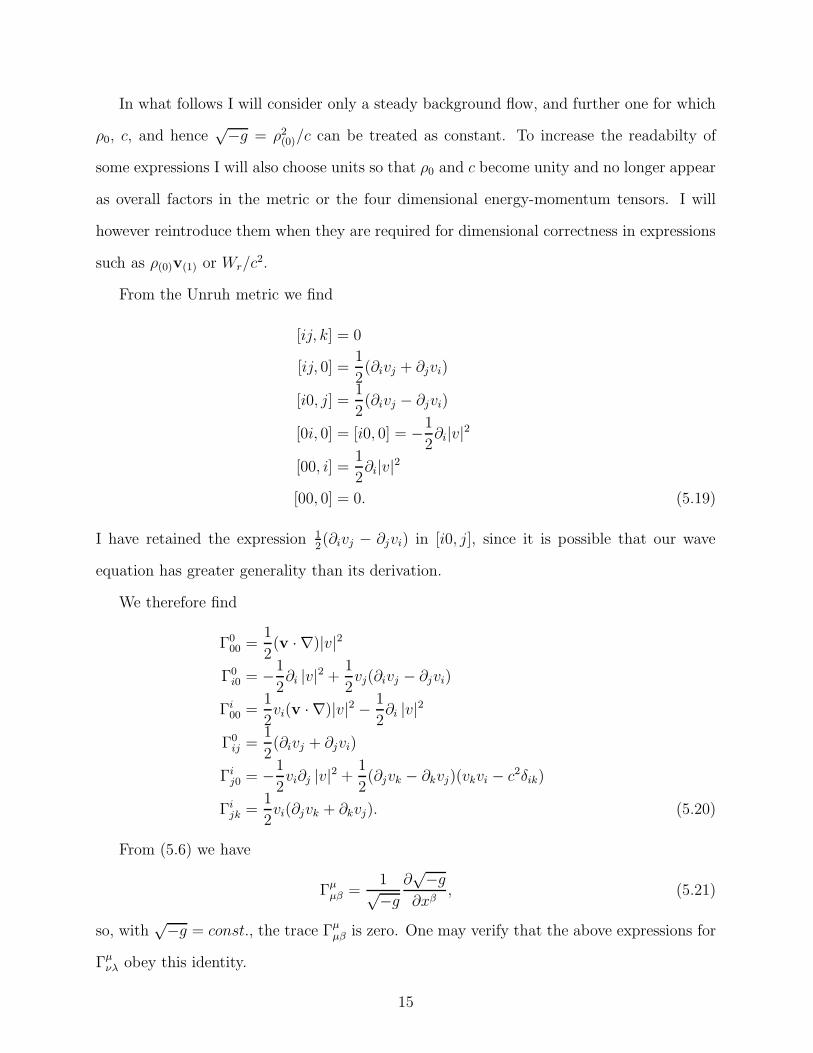
From the Unruh metric we find

[ij, k] = 0

[ij, 0] =1

2(∂ivj + ∂jvi)

[i0, j] =1

2(∂ivj − ∂jvi)

[0i, 0] = [i0, 0] = −1

2∂i|v|2

[00, i] =1

2∂i|v|2

[00, 0] = 0. (5.19)

I have retained the expression 12(∂ivj − ∂jvi) in [i0, j], since it is possible that our wave

equation has greater generality than its derivation.

We therefore find

Γ000 =

1

2(v · ∇)|v|2

Γ0i0 = −1

2∂i |v|2 +

1

2vj(∂ivj − ∂jvi)

Γi00 =

1

2vi(v · ∇)|v|2 − 1

2∂i |v|2

Γ0ij =

1

2(∂ivj + ∂jvi)

Γij0 = −1

2vi∂j |v|2 +

1

2(∂jvk − ∂kvj)(vkvi − c2δik)

Γijk =

1

2vi(∂jvk + ∂kvj). (5.20)

From (5.6) we have

Γµµβ =

1√−g

∂√−g

∂xβ, (5.21)

so, with√−g = const., the trace Γµ

µβ is zero. One may verify that the above expressions for

Γµνλ obey this identity.

15

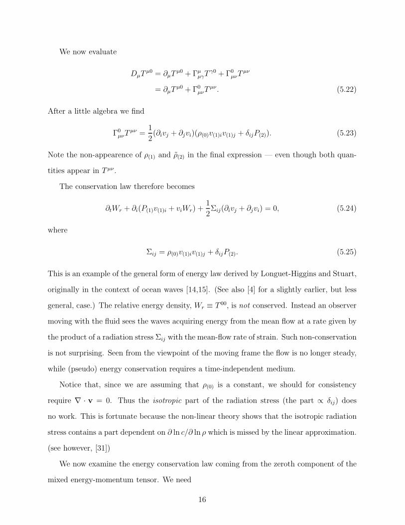
We now evaluate

DµTµ0 = ∂µT

µ0 + ΓµµγT

γ0 + Γ0µνT

µν

= ∂µTµ0 + Γ0

µνTµν . (5.22)

After a little algebra we find

Γ0µνT

µν =1

2(∂ivj + ∂jvi)(ρ(0)v(1)iv(1)j + δijP(2)). (5.23)

Note the non-appearence of ρ(1) and ρ(2) in the final expression — even though both quan-

tities appear in T µν .

The conservation law therefore becomes

∂tWr + ∂i(P(1)v(1)i + viWr) +1

2Σij(∂ivj + ∂jvi) = 0, (5.24)

where

Σij = ρ(0)v(1)iv(1)j + δijP(2). (5.25)

This is an example of the general form of energy law derived by Longuet-Higgins and Stuart,

originally in the context of ocean waves [14,15]. (See also [4] for a slightly earlier, but less

general, case.) The relative energy density, Wr ≡ T 00, is not conserved. Instead an observer

moving with the fluid sees the waves acquiring energy from the mean flow at a rate given by

the product of a radiation stress Σij with the mean-flow rate of strain. Such non-conservation

is not surprising. Seen from the viewpoint of the moving frame the flow is no longer steady,

while (pseudo) energy conservation requires a time-independent medium.

Notice that, since we are assuming that ρ(0) is a constant, we should for consistency

require ∇ · v = 0. Thus the isotropic part of the radiation stress (the part ∝ δij) does

no work. This is fortunate because the non-linear theory shows that the isotropic radiation

stress contains a part dependent on ∂ ln c/∂ ln ρ which is missed by the linear approximation.

(see however, [31])

We now examine the energy conservation law coming from the zeroth component of the

mixed energy-momentum tensor. We need

16

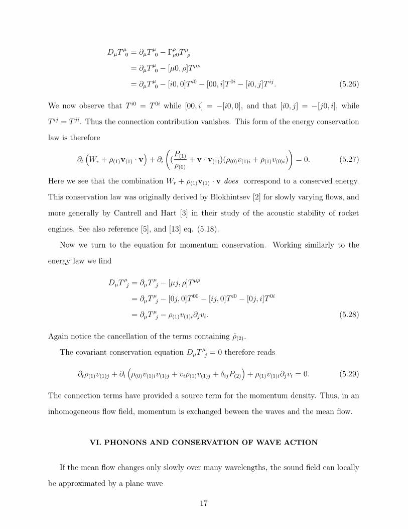
DµTµ0 = ∂µT

µ0 − Γρ

µ0Tµρ

= ∂µTµ0 − [µ0, ρ]T µρ

= ∂µTµ0 − [i0, 0]T i0 − [00, i]T 0i − [i0, j]T ij. (5.26)

We now observe that T i0 = T 0i while [00, i] = −[i0, 0], and that [i0, j] = −[j0, i], while

T ij = T ji. Thus the connection contribution vanishes. This form of the energy conservation

law is therefore

∂t(

Wr + ρ(1)v(1) · v)

+ ∂i

(

(P(1)

ρ(0)+ v · v(1))(ρ(0)v(1)i + ρ(1)v(0)i)

)

= 0. (5.27)

Here we see that the combination Wr + ρ(1)v(1) · v does correspond to a conserved energy.

This conservation law was originally derived by Blokhintsev [2] for slowly varying flows, and

more generally by Cantrell and Hart [3] in their study of the acoustic stability of rocket

engines. See also reference [5], and [13] eq. (5.18).

Now we turn to the equation for momentum conservation. Working similarly to the

energy law we find

DµTµj = ∂µT

µj − [µj, ρ]T µρ

= ∂µTµj − [0j, 0]T 00 − [ij, 0]T i0 − [0j, i]T 0i

= ∂µTµj − ρ(1)v(1)i∂jvi. (5.28)

Again notice the cancellation of the terms containing ρ(2).

The covariant conservation equation DµTµj = 0 therefore reads

∂tρ(1)v(1)j + ∂i(

ρ(0)v(1)iv(1)j + viρ(1)v(1)j + δijP(2)

)

+ ρ(1)v(1)i∂jvi = 0. (5.29)

The connection terms have provided a source term for the momentum density. Thus, in an

inhomogeneous flow field, momentum is exchanged beween the waves and the mean flow.

VI. PHONONS AND CONSERVATION OF WAVE ACTION

If the mean flow changes only slowly over many wavelengths, the sound field can locally

be approximated by a plane wave

17

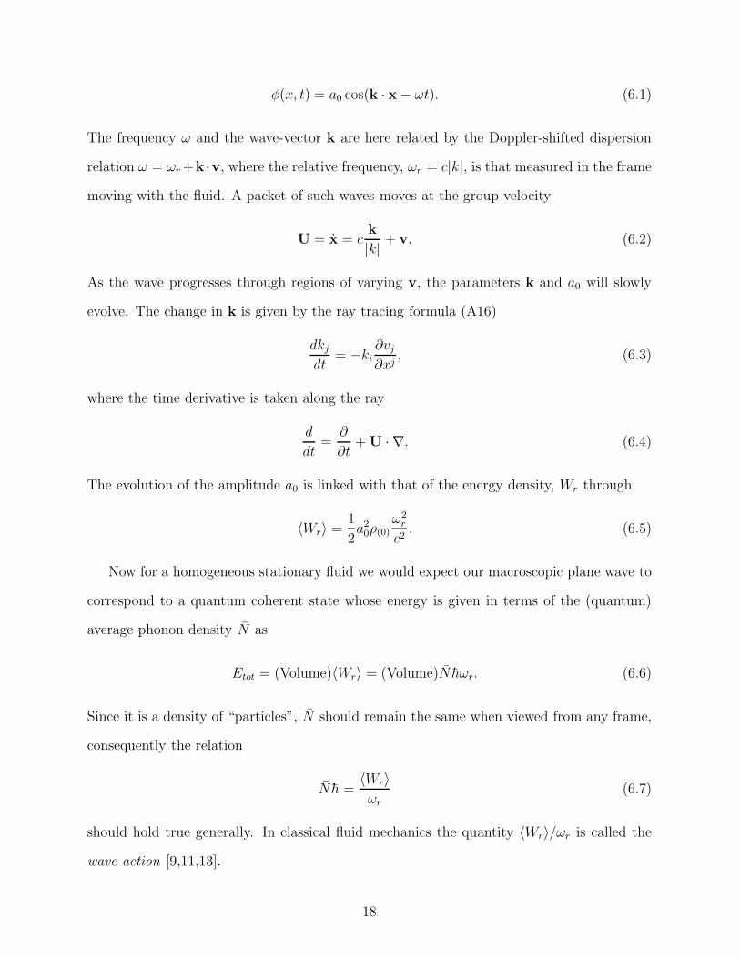
φ(x, t) = a0 cos(k · x− ωt). (6.1)

The frequency ω and the wave-vector k are here related by the Doppler-shifted dispersion

relation ω = ωr+k ·v, where the relative frequency, ωr = c|k|, is that measured in the frame

moving with the fluid. A packet of such waves moves at the group velocity

U = x = ck

|k| + v. (6.2)

As the wave progresses through regions of varying v, the parameters k and a0 will slowly

evolve. The change in k is given by the ray tracing formula (A16)

dkjdt

= −ki∂vj∂xj

, (6.3)

where the time derivative is taken along the ray

d

dt=

∂

∂t+U · ∇. (6.4)

The evolution of the amplitude a0 is linked with that of the energy density, Wr through

〈Wr〉 =1

2a20ρ(0)

ω2r

c2. (6.5)

Now for a homogeneous stationary fluid we would expect our macroscopic plane wave to

correspond to a quantum coherent state whose energy is given in terms of the (quantum)

average phonon density N as

Etot = (Volume)〈Wr〉 = (Volume)Nhωr. (6.6)

Since it is a density of “particles”, N should remain the same when viewed from any frame,

consequently the relation

Nh =〈Wr〉ωr

(6.7)

should hold true generally. In classical fluid mechanics the quantity 〈Wr〉/ωr is called the

wave action [9,11,13].

18

The time averages of other components of the energy momentum tensor may be also

expressed in terms of N . For the mixed tensor we have

〈T 00〉 = 〈Wr + v · ρ(1)v(1)〉 = Nhω

〈T i0〉 = 〈(P(1)

ρ(0)+ v · v(1))(ρ(0)v(1)i + ρ(1)vi)〉 = NhωUi

〈−T 0i〉 = 〈ρ(1)v(1)i〉 = Nhki

〈−T ij〉 = 〈ρ(0)v(1)iv(1)j + viρ(1)v(1)j + δijP(2)〉 = NhkjUi. (6.8)

The last result uses the fact that 〈P(2)〉 = 0 for a plane progressive wave.

Inserting these approximate expressions for the time averages into the Blokhintsev energy

conservation law (5.27) we find that

∂Nhω

∂t+∇ · (NhωU) = 0. (6.9)

We can write this as

Nh

(

∂ω

∂t+U · ∇ω

)

+ hω

(

∂N

∂t+∇ · (NU)

)

= 0. (6.10)

The first term is equal to dω/dt along the rays and vanishes for a steady mean flow as a

consequence of the hamiltonian nature of the ray tracing equations. The second term must

therefore also vanish. This represents the conservation of phonons, or in classical language,

the conservation of wave-action.

In a similar manner the time average of (5.28) may be written

0 =∂Nkj∂t

+∇ · (NkjU) + Nki∂vi∂xj

= N

(

∂kj∂t

+U · ∇kj + ki∂vi∂xj

)

+ kj

(

∂N

∂t+∇ · (NU)

)

. (6.11)

We see therefore that the momentum law is equivalent to phonon-number conservation

combined with the ray tracing equation (A16).

VII. DISCUSSION

The possibilty of interpreting the time average of our momentum conservation law in

terms of quantum quasi-particles should warn us that we are dealing with pseudomomentum

19

and not with newtonian momentum [18]. Nonetheless the quantity 〈ρ(1)v(1)〉 = Nhk is

reliably computed from the linearized wave equation, and is part of the true momentum.

It is simply not all of it. Even in the absence of a mean flow with its 〈ρ(2)v〉 contribution

we still have to contend with ρ(0)〈v(2)〉, and this can be important. As an example [18],

consider a closed cylinder filled with fluid. At one end of the cylinder a piston is driven

so as to generate plane sound waves which completely span the cross section of the tube.

At the other end a second piston is driven at the same frequency with its phase adjusted

so as to absorb the sound waves without reflection. It easy to see that an extra pressure

equal to 〈Wr〉 is exerted on the ends of the tube over and above whatever isotropic pressure

acts on the ends and sides equally. It is “obvious” that this is the force per unit area Nhkc

required to generate and absorb the phonon beam “momentum”. Unfortunately for this

simple idea, it is equally obvious that the time average center-of-mass velocity of the fluid in

the tube vanishes, so the true momentum density in the beam is exactly zero. The 〈ρ(1)v(1)〉

contribution to the momentum density is exactly cancelled by a ρ(0)〈v2〉 counterflow. This

eulerian streaming is driven by the fluid source term for 〈v(2)〉 implicit in (5.16) [30]. (In a

lagrangian description the particles merely oscillate back and forth with no secular drift).

The momentum flux however is exactly the same as if (the italics are from [18]) there was

no medium and the phonons were particles possessing momentum hk. This is frequently

true: the flux of pseudomomentum is often equal to the flux of true momentum to O(a2)

accuracy. Pseudomomentum flux can therefore be used to compute forces. On the other

hand the density of true momentum in the fluid and the density of pseudomomentum are

usually unrelated2.

2This does not mean that the attribution of momentum to a phonon in the two-fluid model for

a superfluid is incorrect. In superfluid hydrodynamics the ρ(0)〈v2〉 counterflow is accounted for

separately from the 〈ρ(1)v(1)〉 = Nhk normal-component mass flux. The counterflow is included

in the supercurrent needed to enforce ∇ · (ρnvn + ρsvs) = 0.

20

It should be said that the ρ(0)〈v2〉 counterflow will not always cancel the ρ(1)〈v1〉 wave

pseudomomentum [33]. The 〈v2〉 flow depends the geometry. It is found from the source

equation (5.16) and from the force the sound field applies to the fluid. The latter will

be small when there is no dissipation, as is the case in a superfluid, and for an isolated

sound beam source in an infinite medium 〈v2〉 will consist of a flow directed radially inwards

towards the transducer of sufficient magnitude to supply the mass flowing out along the

sound beam [30]. In the presence of dissipation the force becomes important, leading to

acoustic streaming.

Consider our closed cylinder further. From (4.13) we see that in a system with fixed 〈P 〉,

and in the presence of the sound wave, the mean density of the fluid will be reduced by

〈ρ(2)〉 = −〈Wr〉c2

d ln c

d ln ρ

∣

∣

∣

∣

∣

ρ(0)

. (7.1)

Since our cylinder has fixed volume, this density reduction cannot take place. Instead it is

opposed by a pressure on the cylinder wall

∆P = 〈Wr〉d ln c

d ln ρ

∣

∣

∣

∣

∣

ρ(0)

, (7.2)

that must be added to the isotropic pressure in the absence of the sound wave. The complete

radiation stress tensor is therefore

〈Σij〉 = 〈Wr〉(

kikjk2

+ δijd ln c

d ln ρ

)

. (7.3)

This result goes back to Brillouin [32]. The true radiation stress therefore differs from the

pseudomomentum flux tensor in its isotropic part. Forces computed from pseudomomentum

flux will therefore be incorrect if this pressure gradient is important. Usually it is not. See

[34] for examples.

VIII. ACKNOWLEDGEMENTS

This work was supported by grant NSF-DMR-98-17941. I would like to thank Edouard

Sonin, David Thouless, and Ping Ao for many discussions, and Stefan Llewellyn-Smith for

useful e-mail.

21

APPENDIX A: GEODESICS AND HAMILTONIAN FLOWS

In this appendix we show that the null geodesics of the Unruh metric coincide with

conventional hamiltonian optics ray tracing. The usual ray tracing equations are derived

from ω(k,x) as

x =∂ω

∂k, k = −∂ω

∂x. (A1)

In our case ω(k,x) = c|k|+ v · k. Thus

dxi

dt= vi + c

ki|k| ,

dkidt

= −∂vj∂xi

kj. (A2)

We begin by noting that geodesics with an affine parameter τ are stationary paths for

the lagrangian

L =1

2gµν

dxµ

dτ

dxν

dτ. (A3)

To make connection with the ray tracing formalism we consider the corresponding hamilto-

nian

H =1

2gµνpµpν , (A4)

and write down Hamilton’s equations with τ playing the role of time

dxµ

dτ=

∂H

∂pµ= gµνpν

dpµdτ

= − ∂H

∂xµ= −1

2

∂gαβ

∂xµpαpβ. (A5)

Combining these gives

d2xµ

dτ 2=

∂gµβ

∂xα

dxα

dτpµ + gµν

(

−1

2

∂gαβ

∂xν

)

pαpβ. (A6)

Now for matrices g we have

dg−1 = −g−1(dg)g−1, (A7)

so with (g)αβ = gαβ and (g−1)αβ = gαβ we can write

22

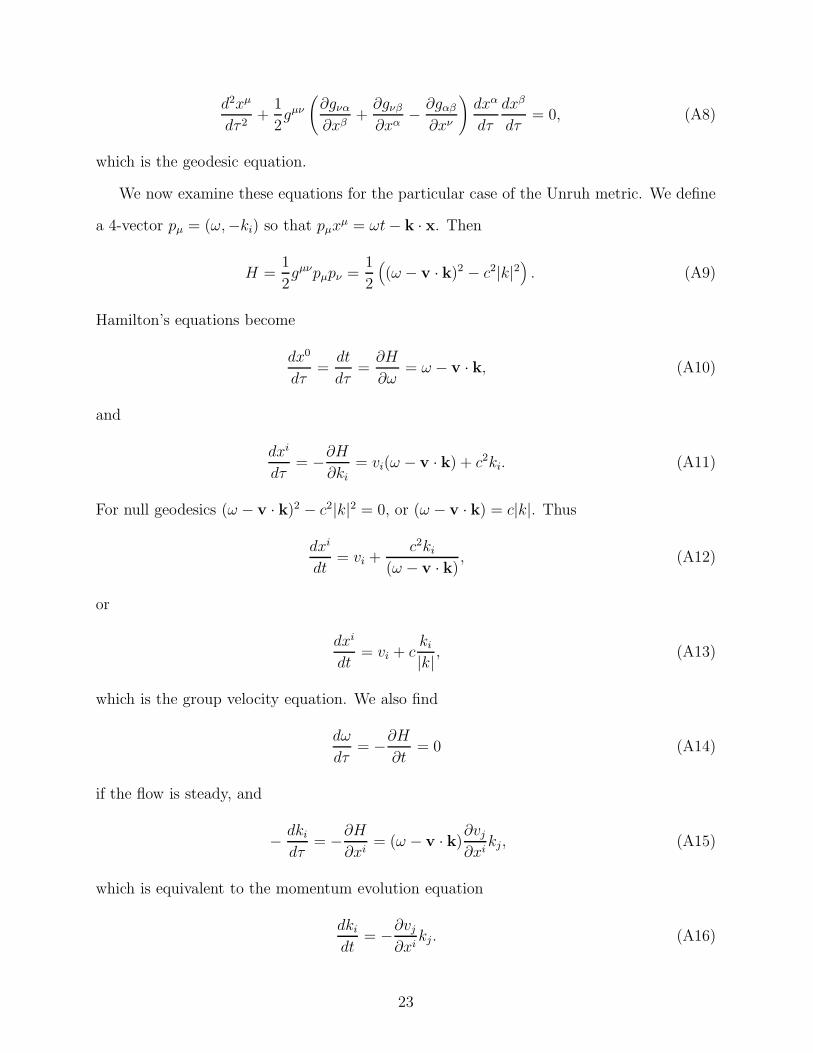
d2xµ

dτ 2+

1

2gµν

(

∂gνα∂xβ

+∂gνβ∂xα

− ∂gαβ∂xν

)

dxα

dτ

dxβ

dτ= 0, (A8)

which is the geodesic equation.

We now examine these equations for the particular case of the Unruh metric. We define

a 4-vector pµ = (ω,−ki) so that pµxµ = ωt− k · x. Then

H =1

2gµνpµpν =

1

2

(

(ω − v · k)2 − c2|k|2)

. (A9)

Hamilton’s equations become

dx0

dτ=

dt

dτ=

∂H

∂ω= ω − v · k, (A10)

and

dxi

dτ= −∂H

∂ki= vi(ω − v · k) + c2ki. (A11)

For null geodesics (ω − v · k)2 − c2|k|2 = 0, or (ω − v · k) = c|k|. Thus

dxi

dt= vi +

c2ki(ω − v · k) , (A12)

or

dxi

dt= vi + c

ki|k| , (A13)

which is the group velocity equation. We also find

dω

dτ= −∂H

∂t= 0 (A14)

if the flow is steady, and

− dkidτ

= −∂H

∂xi= (ω − v · k)∂vj

∂xikj, (A15)

which is equivalent to the momentum evolution equation

dkidt

= −∂vj∂xi

kj. (A16)

23

REFERENCES

[1] P. M. Morse, K. U. Ingard, in Handbuch der Physik Vol XI/1., S. Flugge ed. (Springer

Verlag, Berlin 1961).

[2] D. I. Blokhintsev, Acoustics of a Non-homogeneous Moving Medium. (Gostekhizdat,

1945). [English Translation: N. A. C. A. Technical Memorandum no. 1399, (1956)]

[3] R. H. Cantrell, R. W. Hart, J. Acoustical Soc. Amer. 36 (1964) 697.

[4] O. S. Ryshov, G. M. Shefter, Prik. Mat. Mek. 26 (1962) 854 [J. Appl. Math. Mech. 26

(1962) 1293].

[5] C. L. Morfey, J. Sound and Vib. 14 (1971)159.

[6] M. K. Meyers, J. Sound and Vib. 109 (1986)277 .

[7] G. B. Whitham, J. Fluid. Mech. 12 (1962) 135.

[8] G. B. Whitham, J. Fluid. Mech. 22 (1965) 273.

[9] C. J. R. Garrett, Proc. Roy. Soc. A299 (1967) 26.

[10] F. P. Bretherton, C. J. R. Garrett, Proc. Roy. Soc. A302 (1968) 529.

[11] Sir James Lighthill, Waves in Fluids (Cambridge University Press 1978).

[12] D G. Andrews, M. E. McIntyre, J. Fluid. Mech. 89 (1978) 609.

[13] D G. Andrews, M. E. McIntyre, J. Fluid. Mech. 89 (1978) 647.

[14] M. S. Longuet-Higgins, R. W. Stuart, J. Fluid. Mech. 10 (1961) 529.

[15] M. S. Longuet-Higgins, R. W. Stuart, Deep Sea Res. 11 (1964) 529.

[16] M. K. Meyers, J. Fluid. Mech. 226 (1991) 383.

[17] Sir Rudolf Peierls, Surprises in Theoretical Physics , (Princeton, 1979).

[18] M. E. McIntyre, J. Fluid. Mech. 106 (1981) 331.

24

[19] W. Unruh, Phys. Rev. Lett. 46 (1981) 1351.

[20] W. Unruh, Phys. Rev. D 51 (1995) 2827.

[21] Sir Rudolf Peierls, More Surprises in Theoretical Physics , (Princeton, 1991).

[22] C. Wexler, Phys. Rev. Lett. 79 (1997) 1321. (cond-mat/9612111)

[23] C. Wexler, D. J. Thouless, Rev. B58 (1998) 8897. (cond-mat/9804118)

[24] E. B. Sonin, Phys. Rev. B55 (1997) 485. (cond-mat/9606099)

[25] G. E. Volovik Pis’Ma Zhu. Eksp. Teor. Fiz. 67 (1998) 841 [JETP Letters 67 (1998)

pp.881] (cond-mat/9804308)

[26] A. M. J. Schakel, Mod. Phys. Lett. B10 (1996) 999. [cond-mat/9607164]

[27] R. Arnowit, S. Deser, C. W. Misner in Gravitation: an Introduction to Current Re-

search ed. L. Witten (Wiley N.Y. 1962), pp227-265; C. Misner, K. Thorne, J. Wheeler,

Gravitation (W. H. Freeman, San Francisco 1973).

[28] For a picture see C. Misner, K. Thorne, J. Wheeler, op. cit. p504.

[29] S. Weinberg, Gravitation and cosmology: principles and applications of the general the-

ory of relativity. (Wiley, New York, 1972).

[30] Sir James Lighthill, J. Sound and Vib. 61 (1978) 391.

[31] F. P. Bretherton, Mathematical Problems in the Geophysical Sciences , Lectures in Ap-

plied Mathematics, Volume 13 (Am. Math. Soc. , Providence RI, 1971) p61.

[32] L. Brillouin, Annales de Physique, 4 (1925) 528 (in French).

[33] C. S. Yih, J. Fluid. Mech. 331 (1991) 429.

[34] E. J. Post, J. Acoustical Soc. Amer. 25 (1953) 55.

25