Embed Size (px)
Citation preview

ACOUSTIC EMISSION ANALYSIS FOR BEARING CONDITION MONITORING
MOHD HELMI BIN RASID
Report submitted in partial fulfilment of the requirements for the award of
Bachelor of Mechanical Engineering
Faculty of Mechanical Engineering
UNIVERSITI MALAYSIA PAHANG
JUNE 2013

v
ABSTRACT
Acoustic emission (AE) was originally developed for non-destructive testing
of static structures, however, over the years its application has been extended to
health monitoring of rotating machines and bearings. It offers the advantage of
earlier defect detection in comparison to vibration analysis. Current methodologies
of applying AE for bearing diagnosis are reviewed. The investigation reported in
this paper was centered on the application of standard acoustic emissions (AE)
characteristic parameters on a rotational speed. An experimental test-rig was
designed to allow seeded defects on the inner race, corrode and contaminated
defect. It is concluded that irrespective of the rotational speed and high levels of
background noise, simple AE parameters such as amplitude and AE counts
provided an indications of bearing defect. In addition to validating already
established AE techniques, this investigation focuses on establishing an appropriate
threshold level for AE counts.

vi
ABSTRAK
Pelepasan akustik (AE) pada asalnya dibangunkan untuk ujian tidak
memusnahkan struktur statik, bagaimanapun, sejak beberapa tahun permohonan
telah dilanjutkan kepada pemantauan kesihatan mesin dan bearing berputar. Ia
menawarkan kelebihan mengesan kecacatan awal berbanding dengan analisis
getaran. Metodologi semasa memohon AE untuk menanggung diagnosis dikaji
semula. Penyiasatan yang dilaporkan dalam kertas ini berpusat pada permohonan
pelepasan akustik standard (AE) parameter ciri pada kelajuan putaran. Eksperimen
ujian pelantar telah direka untuk membolehkan kecacatan pilihan pada perlumbaan
dalam, mengakis dan tercemar kecacatan. Ia menyimpulkan bahawa tanpa mengira
kelajuan putaran dan tahap bunyi latar belakang, parameter AE mudah seperti
amplitud dan tuduhan AE memberi tanda-tanda kecacatan bearing. Selain
mengesahkan teknik AE telah ditubuhkan, penyiasatan ini memberi tumpuan
kepada mewujudkan tahap ambang yang sesuai bagi tuduhan AE.
vii
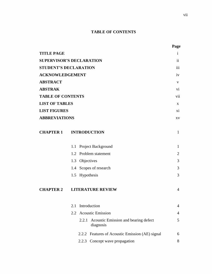
TABLE OF CONTENTS
Page
TITLE PAGE i
SUPERVISOR’S DECLARATION ii
STUDENT’S DECLARATION iii
ACKNOWLEDGEMENT iv
ABSTRACT v
ABSTRAK vi
TABLE OF CONTENTS vii
LIST OF TABLES x
LIST FIGURES xi
ABBREVIATIONS xv
CHAPTER 1 INTRODUCTION 1
1.1 Project Background 1
1.2 Problem statement 2
1.3 Objectives 3
1.4 Scopes of research 3
1.5 Hypothesis 3
CHAPTER 2 LITERATURE REVIEW 4
2.1 Introduction 4
2.2 Acoustic Emission 4
2.2.1 Acoustic Emission and bearing defect
diagnosis
5
2.2.2 Features of Acoustic Emission (AE) signal 6
2.2.3 Concept wave propagation 8

viii
2.2.4 Acoustic Emission signal 8
2.2.5 Acoustic Emission pre-processing 9
2.3 Type of bearing 11
2.3.1 Cylindrical roller bearings 12
2.4 Type of bearing defect 13
2.4.1 Corrode 14
2.4.2 Inner race defect 14
2.4.3 Contaminant 15
2.5 Test Rig 16
CHAPTER 3 METHODOLOGY 20
3.1 Introduction 20
3.2 Project flow chart 20
3.3 Acoustic Emission test setup 22
3.3.1 Testing procedure 22
3.3.2 Test setup 23
3.3.3 Data acquisition system 23
3.4 Data flow analysis 24
CHAPTER 4 RESULT AND DISCUSSION 26
4.1 Introduction 26
4.2 Revolution per second (RPS) of test rig 26
4.3 Amplitude of defect bearing 29
4.4 Counts 37
4.5 Energy Counts 43
4.6 Discussion 50
CHAPTER 5 CONCLUSION 53

ix
5.1 Conclusion 53
5.2 Recommendation 54
REFERENCE 55
APPENDICES

x
LIST OF TABLES
Table No. page
4.1 Data speed tachometer reading 27
4.17 Summarize of the amplitude 36
4.30 Summarize of the count 43
4.41 Summarize of the energy count 50
4.42 Summarize of all parameter 52

xi
LIST OF FIGURES
Figure No. page
2.1 AE signal features 6
2.2 Type of acoustic emission signal 10
2.3 Cylindrical roller bearing schematic 12
2.4 Cylindrical roller bearing 13
2.5 Corrode cylindrical roller bearings 14
2.6 Inner race defect 15
2.7 Contaminant defect (wear) 16
2.8 Schematic diagram housing and shaft design 17
2.9 Diagrams housing design 18
2.10 Diagrams shaft design 18
2.11 Systematic diagram test rig 19
3.1 Flow chart fabricate bearing and design test rig 20

xii
3.2 Flow chart methodology acoustic emission 21
3.3 Test rig setup 24
4.2 Graph 30 % revolution per second (RPS) 27
4.3 Graph 60 % revolution per second (RPS) 28
4.4 Graph 90 % revolution per second (RPS) 28
4.5 Graph healthy bearing at speed 30 % RPS amplitude 29
4.6 Graph healthy bearing at speed 60 % RPS amplitude 30
4.7 Graph healthy bearing at speed 90 % RPS amplitude 30
4.8 Graph contaminated defect 30 % RPS amplitude 31
4.9 Graph contaminated defect 60 % RPS amplitude 31
4.10 Graph contaminated defect 90 % RPS amplitude 32
4.11 Graph corrode defect 30 % RPS amplitude 33
4.12 Graph corrode defect 60 % RPS amplitude 33
4.13 Graph corrode defect 90 % RPS amplitude 34
4.14 Graph inner defect 30 % RPS amplitude 34

xiii
4.15 Graph inner defect 60 % RPS amplitude 35
4.16 Graph inner defect 90 % RPS amplitude 35
4.18 Graph healthy bearing at speed 30 % RPS count 37
4.19 Graph healthy bearing at speed 60 % RPS count 37
4.20 Graph healthy bearing at speed 90 % RPS count 38
4.21 Graph contaminated defect 30 % RPS count 38
4.22 Graph contaminated defect 60 % RPS count 39
4.23 Graph contaminated defect 90 % RPS count 39
4.24 Graph corrode defect 30 % RPS count 40
4.25 Graph corrode defect 60 % RPS count 40
4.26 Graph corrode defect 90 % RPS count 41
4.27 Graph inner defect 30 % RPS count 41
4.28 Graph inner defect 60 % RPS count 42
4.29 Graph inner defect 90 % RPS count 42
4.31 Graph healthy bearing at speed 30 % RPS energy
count
44

xiv
4.32 Graph healthy bearing at speed 60 % RPS energy
count
44
4.33 Graph healthy bearing at speed 90 % RPS energy
count
45
4.34 Graph contaminated defect 30 % RPS energy count 45
4.35 Graph contaminated defect 60 % RPS energy count 46
4.36 Graph contaminated defect 90 % RPS energy count 46
4.37 Graph corrode defect 30 % RPS energy count 47
4.38 Graph corrode defect 60 % RPS energy count 47
4.39 Graph corrode defect 90 % RPS energy count 48
4.40 Graph inner defect 30 % RPS energy count 48
4.41 Graph inner defect 60 % RPS energy count 49
4.42 Graph inner defect 90 % RPS energy count 49

xv
LIST OF ABBREVIATIONS
AE Acoustic Emission
NDT Non Destructive Testing
dB Decibels
N Counts
A Amplitude
D Duration
R Rise Time
COTS Custom off the shelf
MB Megabytes
RPS Revolution Per Second
1
CHAPTER 1
INTRODUCTION
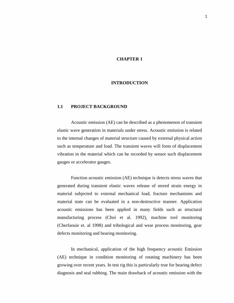
1.1 PROJECT BACKGROUND
Acoustic emission (AE) can be described as a phenomenon of transient
elastic wave generation in materials under stress. Acoustic emission is related
to the internal changes of material structure caused by external physical action
such as temperature and load. The transient waves will form of displacement
vibration in the material which can be recorded by sensor such displacement
gauges or accelerator gauges.
Function acoustic emission (AE) technique is detects stress waves that
generated during transient elastic waves release of stored strain energy in
material subjected to external mechanical load, fracture mechanisms and
material state can be evaluated in a non-destructive manner. Application
acoustic emissions has been applied in many fields such as structural
manufacturing process (Choi et al. 1992), machine tool monitoring
(Cherfaouie et. al 1998) and tribological and wear process monitoring, gear
defects monitoring and bearing monitoring.
In mechanical, application of the high frequency acoustic Emission
(AE) technique in condition monitoring of rotating machinery has been
growing over recent years. In test rig this is particularly true for bearing defect
diagnosis and seal rubbing. The main drawback of acoustic emission with the
2
application of AE technique is the attenuation of the signal and as such the AE
sensor has to be close to its source. In test rig, it is often practical to place
sensor AE on the non-rotating member of the machine such as bearing.
Therefore, the AE signal originating from the defective component will suffer
severe attenuation before reaching the sensor. Usually typical frequencies
associated with AE activity range 20 to 1MHz.
The acoustic emission (AE) method is a high frequency analysis
technique which initially developed as a non destructive testing (NDT) tool to
detect crack growth in material and structure. Now, AE method has been
increasingly being used as condition monitoring tool of engineering assets
such as structures and industrial machines.
In this study, envelop analysis bearing condition monitoring for
detecting of bearing defect in signal process.
1.2 PROBLEM STATEMENT
Acoustic emission is non-destructive testing for detection in rotating
machinery that can be conducted to investigate the acoustic emission response
of defective bearings. In acoustic monitoring is can even detect the growth of
subsurface cracks whereas vibration monitoring can normally detect a defect
when it appears on the surface (Tandon,1990) and in this study we have
attempted to provide corroborative evidence that bearing defect can be
measured and analyzed using acoustic emission method.
In this research was develop fabricate and design bearing used test rig
to investigate the changes acoustic emission signal of simulated defects on the
defect on cylindrical roller bearing and the analysis of the result will do with
this test.

3
1.3 OBJECTIVES
The main objective for this research is:
i. To detect bearing condition using acoustic emission method
1.4 SCOPE OF RESEARCH
For this research, the acoustic emission testing will be done to detect a
signal from test rig. From test rig can used in non-destructive testing for the
detection of defect bearing and failure detection in rotating machinery. The
result from the test will be analyzed according to the acoustic emission
technique.
With different defect of the bearing such as contaminant, corrode and
inner race have different result for acoustic parameter. From this experiment
also want to study the parameter of acoustic emission such as counts and
energy counts and amplitude. Data from acoustic emission parameter will be
analyzed to get the characteristic of acoustic.
1.5 HYPOTHESIS
In this research, some of the hypothesis has done such as:
i. Different defect bearing used in test rig, so the prediction of the result
will get different result from acoustic parameter such as different ring-down
counts, events and peak amplitude of the signals.

4
CHAPTER 2
LITERATURE REVIEW
2.1 INTRODUCTION
The purpose of this chapter is to provide a review of past research
efforts related to acoustic emission testing, type of bearing, type of bearing
defect and mechanical testing that test rig. A review of other relevant research
studies also provides. The review is organized chronologically to offer insight
to how past research efforts have laid the groundwork for subsequent studies,
including the present research effort.
2.2 ACOUSTIC EMISSION
Acoustic emission is defined as generation of transient elastic waves
produced by a sudden redistribution of stress in a material. Detection and
analysis of acoustic emission signal can get valuable information of a
discontinuity in material such as bearing defect (Mathews, 1983). Typical
sources of acoustic emissions include plastic deformation, wear, micro
fracture, bubble collapse, impact and friction. When these waves reach the
surface of the material they can be detected and measured by acoustic
emission sensors. Acoustic emission signals are generally only a few
microvolts to milivolts in amplitude when measured at the sensing element
and range from several kHz to a MHz. At these frequencies, signals are

5
strongly attenuated in air so a suitable couplant is required between the sensor
and material to ensure signal transmission.
2.2.1 Acoustic emission and bearing defect diagnosis
Yoshioka have shown on research state that acoustic parameters
identified bearing defects before they appeared in the vibration acceleration
range whilst Catlin reported acoustic emission activity from bearing defects
were attributed to four main factors, including random noise generated. It was
noted that signals detected in the acoustic emission frequency range
represented bearing defects rather than other defects such as imbalance,
misalignment, looseness and shaft bending.
Tandonet on research investigated acoustic emission counts and peak
amplitudes for an outer race defect using a resonant type transducer. It was
concluded that AE counts increased with increasing load and rotational speed.
However, it was observed that AE counts could only be used for defect
detection when the defect was less than 250μm in diameter; through AE peak
amplitude provided an indication of defects identification on various sized
bearings and rotational speed. It was observed that AE counts were low for
undamaged bearings. In addition, it was observed that AE counts increased
with increasing load and speed for damaged undamaged bearing.
A clear relationship between rms level, rotational speed and radial load
has been reported. The use of AE counts is dependent on the particular
investigation and the method of determining the threshold level is at the
discretion of the investigator. For this reason, the investigation presented in
this paper firstly validates the use of rms for diagnosis and secondly,
ascertains the suitability of AE counts for bearing diagnosis. In addition,
selection of the appropriate threshold level is investigated.

6
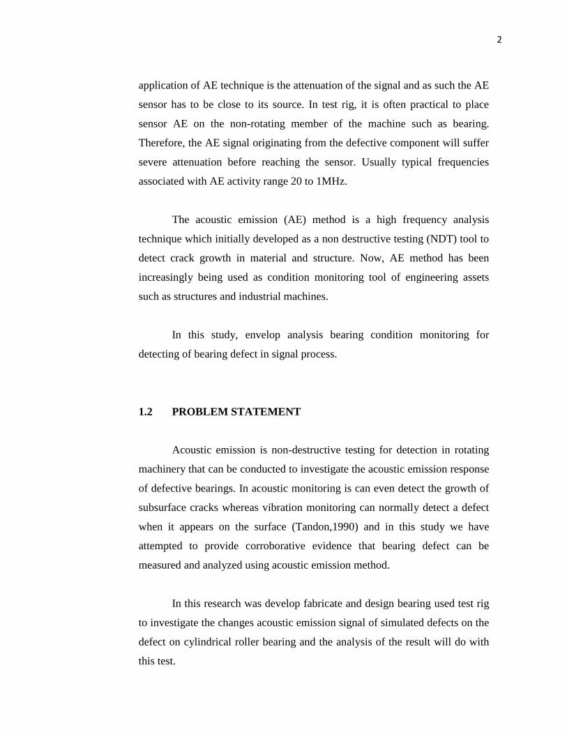
2.2.2 Features of Acoustic Emission (AE) Signal
The commonly measured acoustic emission parameters are counts,
events and peak amplitude of the signal. Ringdown counts involve counting
the number of times the amplitude exceeds a preset voltage (threshold level)
in a given time and gives a simple number characteristic of the signal. An
event consists of a group of ringdown counts and signifies a transient wave.
Each of the AE signal feature shown in the image described below
Figure 2.1: AE signal features
(Source:Yoshioka and Fujiwara, 1984)
Amplitude, A, is the greatest measured voltage in a waveform and is
measured in decibels (dB). This is an important parameter in acoustic
emission inspection because it determines the detectability of the signal.
7
Signals with amplitudes below the operator-defined, minimum threshold will
not be recorded (Yoshioka and Fujiwara, 1984).
Rise time, R, is the time interval between the first threshold crossing and the
signal peak. This parameter is related to the propagation of the wave between
the source of the acoustic emission event and the sensor. Therefore, rise time
is used for qualification of signals and as a criterion for noise filter (Yoshioka
and Fujiwara, 1984).
Duration, D, is the time difference between the first and last threshold
crossings. Duration can be used to identify different types of sources and to
filter out noise. Like counts (N), this parameter relies upon the magnitude of
the signal and the acoustics of the material (Yoshioka and Fujiwara, 1984).
MARSE, E, sometimes referred to as energy counts, is the measure of the
area under the envelope of the rectified linear voltage time signal from the
transducer. This can be thought of as the relative signal amplitude and is
useful because the energy of the emission can be determined. MARSE is also
sensitive to the duration and amplitude of the signal, but does not use counts
or user defined thresholds and operating frequencies. MARSE is regularly
used in the measurements of acoustic emissions (Yoshioka and Fujiwara,
1984).
Counts, N, refers to the number of pulses emitted by the measurement
circuitry if the signal amplitude is greater than the threshold. Depending on
the magnitude of the AE event and the characteristics of the material, one hit
may produce one or many counts. While this is a relatively simple parameter
to collect, it usually needs to be combined with amplitude and/or duration
measurements to provide quality information about the shape of a signal
(Yoshioka and Fujiwara, 1984).

8
2.2.3 Concept wave propagation
The main deficiency of this analysis is that the wave propagation
through the structure exhibits several dispersive wave modes. Due to the
characteristics of propagation of these wave modes, there are certain
characteristic frequency ranges that propagate with sufficient magnitude to be
sensed by the AE sensors. These frequency ranges vary as a function of
structural properties and geometry even when the damage mechanism is
identical (Tandon, 1990). Thus, it is not reasonable to directly associate
certain AE signal frequency ranges with certain damage mechanisms in a way
that is independent of the material and geometry of the structure. None of
these AE signal analysis techniques used in laboratory studies has proven to
be capable of consistently dealing with the difficulties encountered in large
structure, namely, large amounts of data, the elimination of noise sources,
material anisotropy, and the influence of wave propagating effects
(attenuation and dispersion). These analyses often gave controversial results
because they lack a physical justification (based on the theory of AE) for the
signal features used to sort the experimental signals into different source
mechanisms.
2.2.4 Acoustic Emission signal
AE signals is a characteristic of the process which produces it. Hence
the AE signals contain information about the AE source, which includes
location, magnitude, and damage mechanisms; the structure through which
the wave propagates in the form of transient stress waves; and the monitoring
system including the sensor (i.e., piezoelectric sensors) either mounted on or
embedded in the structure and the associated signal processing electronics.
With the ever increasing power of data acquisition systems and the increased
sensitivity of new sensors, recording the entire waveform with high fidelity
becomes feasible. This waveform approach characterizes AE signals by

9
employing transient wave theory to predict the signals generated by different
types of damage mechanisms. This, in turn, enables experimentally measured
acoustic emission data to be interpreted in a physically meaningful manner.
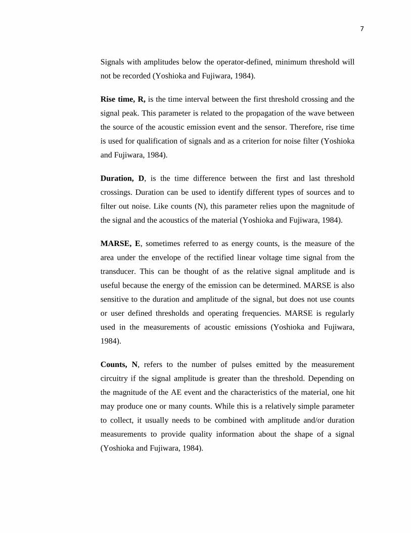
2.2.5 Acoustic emission pre-processing
AE pre-processing involves amplification and filtering to refine the
bandwidth and avoid aliasing. Signals are characterized as continuous, burst
or mixed mode. Continuous emissions are burst that occur too closely together
to differentiate between individual events, appearing as an increase in the
background signal level. They typically have no distinguishing features other
than their amplitude and frequency content. Burst emissions are typically
discrete transients with relatively short decay times and even shorter rise
times. Last is mixed mode AE contains a number of large individual burst
above a background emissions. As most AE is broadband, processing is
usually done in the time domain.
Hits and events are important concept to traditional AE signal analysis.
A hit is defined as AE burst that exceeds a certain voltage threshold.
Generally speaking, an event occurs when the peak voltage remains above the
threshold for consecutive hits. Both hit and event date features are therefore a
function of the type and value of the selected threshold (Bansal, 1990).
Thresholds are referred to as fixed, in which case they are set to an absolute
value for the duration of the rest or floating, where the threshold level is set as
a defined amount (a fixed voltage or fixed number of standard deviation)
above the background level. Fixed thresholds are typically used when
monitoring static equipment, whilst rotating machinery requires floating
thresholds to avoid swamping acquisition hardware when fluctuations in
operating conditions cause the background signal level to rise. Unfortunately,
the ability of COTS (custom off the shelf) AE hardware to manipulate

10
thresholds is limited. Modern AE systems are theoretically capable of
detecting and analyzing up to 20,000 hits per second.
Whilst hit features are extracted from a sensor’s amplified filtered
voltage output, continuous signal descriptors are generally extracted from the
signal envelope or from filtered, digitalized waveforms. The number of
simultaneous waveforms that can be collected depends on the amount of data,
which is a function of acquisition rate and resolution, and the acquisition
system’s digital bandwidth: 4 channels of 16-bit waveform data, collected at
5MHz, will result in 40 megabytes (MB) of data per second. This data must
pass across the computer’s PCI bus to the hard disk for storage. Hard disk is
typically restricted to writing data at approximately 40MB per second. As a
result, undertaking multi-channel AE data acquisition consumes a large
proportion of the computing power available in standard desktops and
portable computers. It is therefore difficult to perform real-time advanced
signal analysis of digitalized waveforms, such as discrete-wavelet or short-
time-frequency transformation, on unoptimized consumer-grade- hardware
Figure 2.2: Type of acoustic emission signal
(Source: Yoshioka and Fujiwara, 1984)

11
2.3 TYPE OF BEARING
In experiment test rig, type of bearing use is cylindrical rolling
bearings. Rolling bearings come in many shape and varieties, each with its
own distinctive features. However, when compared with sliding bearings,
rolling bearings all have the following advantages:
i. The starting friction coefficient is lower and there is little difference
between this and the dynamic friction coefficient.
ii. They are internationally standardized, interchangeable and readily
obtainable.
iii. They are easy to lubricate and consume less lubricant
iv. As a general rule, one bearing can carry both radial and axial loads at
the same time
v. Maybe used either high or low temperature applications.
vi. Bearing rigidity can be improved by preloading.
Most rolling bearing consist of rings with raceway (inner ring and
outer ring), roller and cage. The cage separates the rolling element at regular
intervals, holds them in place within the inner and outer raceways and allows
them to rotate freely. The surface on the rolling element roll is called the
“raceway surface”. The load placed on the bearing is supported by this contact
surface. Generally the inner ring fits on the axle or shaft and the outer ring on
the housing. Theoretically, rolling bearing are so constructed as to allow the
rolling elements to rotate orbitally while also rotating on their own axes at the
same time. The function of cages bearing is to maintain rolling elements at a
uniform pitch so load is never applied directly to the cage and to prevent the
rolling element from falling out when handling the bearing.
Rollers bearing on the other hand are classified according to the shape
of the rollers; cylindrical, needle, tapered and spherical. Rolling bearings can

12
be further classified according to the direction in which the load is applied;
radial bearings carry radial loads and thrust bearings carry axial loads.
2.3.1 Cylindrical roller bearings
In our study, we used cylindrical roller type NU203. Cylindrical roller
bearing uses rollers for rolling elements, and therefore has a high load
capacity. The rollers are guided by the ribs of the inner or outer ring. The
inner and outer rings can be separated to facilitate assembly and both can be
fit with shaft or housing tightly. If there are no ribs, either the inner or the
outer ring can move freely in the axial direction. Cylindrical roller bearings
are therefore ideal to be used as so-called “free side bearings” that absorb
shaft expansion. In the case where there is a rib, the bearing can bear a slight
axial load between the end of the rollers and the ribs. Cylindrical roller
bearings include the HT type which modifies the shape of roller end face and
ribs for increasing axial load capacity. And the E type standardized for small-
diameter sizes.
Figure 2.3: Cylindrical roller bearing schematic
(Source:Tandon. and Nakra, 1990)