A climate, land-use, energy and waternexus assessment of Bolivia

Author: Christopher Arderne

Supervisor: Mark Howells

June 2016

EGI_2016-028MSCMaster of ScienceThesis

KTH School of Industrial Engineering and ManagementDivision of Energy Systems Analysis

SE-100 44 Stockholm

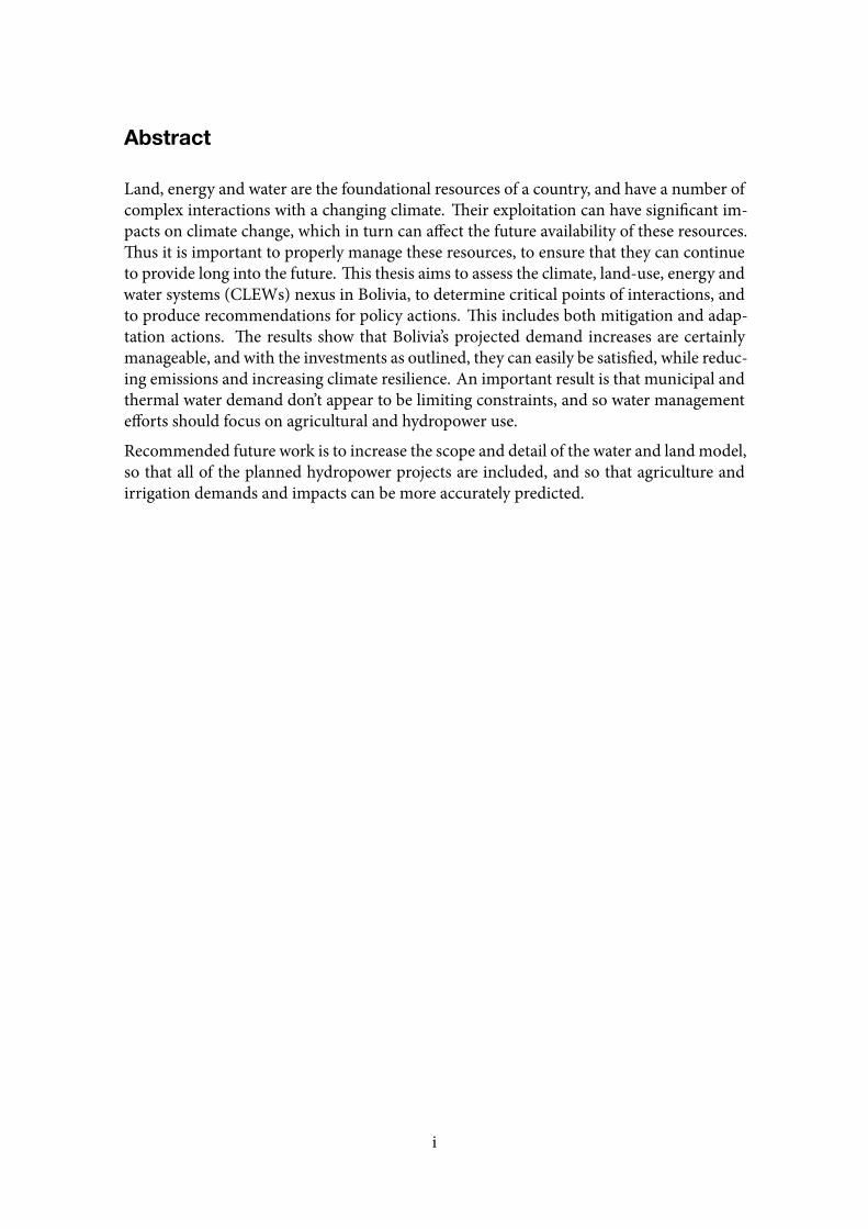
Abstract

Land, energy and water are the foundational resources of a country, and have a number ofcomplex interactions with a changing climate. Their exploitation can have significant im-pacts on climate change, which in turn can affect the future availability of these resources.Thus it is important to properly manage these resources, to ensure that they can continueto provide long into the future. This thesis aims to assess the climate, land-use, energy andwater systems (CLEWs) nexus in Bolivia, to determine critical points of interactions, andto produce recommendations for policy actions. This includes both mitigation and adap-tation actions. The results show that Bolivia’s projected demand increases are certainlymanageable, and with the investments as outlined, they can easily be satisfied, while reduc-ing emissions and increasing climate resilience. An important result is that municipal andthermal water demand don’t appear to be limiting constraints, and so water managementefforts should focus on agricultural and hydropower use.

Recommended future work is to increase the scope and detail of the water and land model,so that all of the planned hydropower projects are included, and so that agriculture andirrigation demands and impacts can be more accurately predicted.

i

Acknowledgements

Thanks toMarkHowells for inspiringmy interest in energymodelling and lettingme workwith dESA for my thesis.

Thanks to Eunice, Vignesh, Dimitris, Oliver and Alex for providing guidance and lots ofhelp. And to some of them thanks for providing endless distractions with other projectsand ideas.

Thanks also to Nandi for being a fantastic and supportive co-researcher.

This thesis was made possible thanks to a Swedish Institute scholarship.

ii

Contents

List of Figures v

List of Tables vi

1 Introduction 11.1 Background . . . . . . . . . . . . . . . . . . . . . . . . . . . . . . . . . . 11.2 Objectives . . . . . . . . . . . . . . . . . . . . . . . . . . . . . . . . . . . 1

2 The CLEWs nexus in Bolivia 22.1 The Bolivian context . . . . . . . . . . . . . . . . . . . . . . . . . . . . . 2

2.1.1 Climate impacts and projections . . . . . . . . . . . . . . . . . . 32.1.2 Land use and food production . . . . . . . . . . . . . . . . . . . 32.1.3 The energy system . . . . . . . . . . . . . . . . . . . . . . . . . . 42.1.4 Water resources . . . . . . . . . . . . . . . . . . . . . . . . . . . 5

3 Methodology 63.1 Overview . . . . . . . . . . . . . . . . . . . . . . . . . . . . . . . . . . . 63.2 Pre-nexus assessment . . . . . . . . . . . . . . . . . . . . . . . . . . . . 73.3 Spatial electrification . . . . . . . . . . . . . . . . . . . . . . . . . . . . . 7

3.3.1 Data gathering and processing . . . . . . . . . . . . . . . . . . . 83.3.2 Electrification and technology costs . . . . . . . . . . . . . . . . 10

3.4 Energy system optimisation . . . . . . . . . . . . . . . . . . . . . . . . . 123.4.1 Reference energy system . . . . . . . . . . . . . . . . . . . . . . 123.4.2 Data sources . . . . . . . . . . . . . . . . . . . . . . . . . . . . . 133.4.3 Electricity demand and emissions . . . . . . . . . . . . . . . . . 14

3.5 Water resources and land use . . . . . . . . . . . . . . . . . . . . . . . . 143.5.1 Basin delineation . . . . . . . . . . . . . . . . . . . . . . . . . . 153.5.2 Assumptions and limitations . . . . . . . . . . . . . . . . . . . . 163.5.3 Catchments, land-use and demand sites . . . . . . . . . . . . . . 183.5.4 Model calibration . . . . . . . . . . . . . . . . . . . . . . . . . . 18

3.6 Scenarios . . . . . . . . . . . . . . . . . . . . . . . . . . . . . . . . . . . 193.6.1 Demand projections . . . . . . . . . . . . . . . . . . . . . . . . . 203.6.2 Climate change . . . . . . . . . . . . . . . . . . . . . . . . . . . 20

3.7 Model integration and interconnections . . . . . . . . . . . . . . . . . . 21

iii

4 Results 234.1 Spatial electrification results . . . . . . . . . . . . . . . . . . . . . . . . . 23

4.2 Energy optimisation results . . . . . . . . . . . . . . . . . . . . . . . . . 26

4.3 Water modelling results . . . . . . . . . . . . . . . . . . . . . . . . . . . 30

5 Conclusions 32

6 Discussion 33

Appendix A Python code: ONSSET data extraction 35

Appendix B Python code: determine hydro potential 41

Appendix C Python code: determining grid connections 43

iv

List of Figures

1 Basic geopolitical overview of Bolivia . . . . . . . . . . . . . . . . . . . . 5

2 Methodological sequence and feedbacks . . . . . . . . . . . . . . . . . . 7

3 ONSSET methodology . . . . . . . . . . . . . . . . . . . . . . . . . . . . 8

4 Renewable energy potential . . . . . . . . . . . . . . . . . . . . . . . . . 10

5 Reference energy system . . . . . . . . . . . . . . . . . . . . . . . . . . 13

6 Electricity demand forecast . . . . . . . . . . . . . . . . . . . . . . . . . 15

7 Primary basins used in WEAP analysis, with planned power plants . . . . 16

8 Results of WEAP calibration . . . . . . . . . . . . . . . . . . . . . . . . 19

9 Calibration example forRioGrande at the site of plannedRositas hydropowerproject . . . . . . . . . . . . . . . . . . . . . . . . . . . . . . . . . . . . 19

10 Different demand projections for population and energy demand . . . . 20

11 Projected rainfall changes per basin, relative to year average of 2000s . . . 21

12 Model links and feedbacks . . . . . . . . . . . . . . . . . . . . . . . . . 22

13 Geospatial technology split . . . . . . . . . . . . . . . . . . . . . . . . . 24

14 Levelised cost of electricity and incidence of extreme poverty by munici-pality . . . . . . . . . . . . . . . . . . . . . . . . . . . . . . . . . . . . . 25

15 Optimal energy capacity mix for baseline . . . . . . . . . . . . . . . . . . 27

16 LCOE and production percentage by source . . . . . . . . . . . . . . . . 28

17 Energy capacity installations relative to baseline . . . . . . . . . . . . . . 28

18 Yearly greenhouse gas emissions and electricity production, relative to non-climate scenarios . . . . . . . . . . . . . . . . . . . . . . . . . . . . . . . 29

19 Water demand by sector . . . . . . . . . . . . . . . . . . . . . . . . . . . 31

20 Monthly capacity factor for selected hydropower plants . . . . . . . . . . 31

v

List of Tables

1 Comparison of SDG indicators . . . . . . . . . . . . . . . . . . . . . . . 3

2 Data used in ONSSET with sources . . . . . . . . . . . . . . . . . . . . . 9

3 Sources for various technology costs . . . . . . . . . . . . . . . . . . . . 11

4 Data sources for OSeMOSYS model . . . . . . . . . . . . . . . . . . . . . 14

5 Main elements in water model . . . . . . . . . . . . . . . . . . . . . . . . 17

6 Data layers used in water system modelling . . . . . . . . . . . . . . . . . 18

7 Total change in annualwater availabilitywith climate changemodelCSIROMk2 B2 . . . . . . . . . . . . . . . . . . . . . . . . . . . . . . . . . . . . 22

8 Technology choice for different scenarios . . . . . . . . . . . . . . . . . . 25

9 Total investment costs . . . . . . . . . . . . . . . . . . . . . . . . . . . . 26

10 Financial breakdown of different scenarios . . . . . . . . . . . . . . . . . 30

11 Change in hydropower capacity factors with climate impacts . . . . . . . 32

vi

List of Abbreviations

BAU Business as usual

CLEWs Climate, Land, Energy and Water systems

FAO Food and Agriculture Organisation of the United Nations

GAEZ Global Agro-Ecological Zones

GDP Gross Domestic Product

GHG Greenhouse gas

GIS Geographical Information Systems

GLPK GNU Linear Programming Kit

HDI Human Development Index

IIASA International Institute for Applied Systems Analysis

KTH-dESA The Division for Energy Systems Analysis at the Royal Instituteof Technology

LCOE Levelised cost of electricity

LHV Lower heating value

LULUCF Land use, land-use change and forestry

MoManI Model Management Infrastructure for OSeMOSYS

ONSSET OpeN Source Spatial Electrification Toolkit

OSeMOSYS Open Source Energy Modeling System

O&M Operation and maintenance

PP Power plant

PV Photovoltaic

RES Reference energy system

SDG Sustainable Development Goal

UN DESA United Nations Department of Economic and Social Affairs

VBA Visual Basic for Applications

WEAP Water Evaluation and Planning

vii

1 Introduction

1.1 Background

With increasing standards of living and populations, the world places increasing stresseson its key resources. Competition for water resources, access to quality land, and afford-able energy availability are at the core of this issue. And as the use and misuse of theseresources contributes to climate change, so the changing climate makes their continueduse more unpredictable and prone to instability. These issues are particularly pressing indeveloping countries, which have less developed infrastructure, and the systems are morevulnerable and less able to adapt. On top of this, global electricity access levels remain low,water access is often rudimentary and land and malnourishment issues persist. Thus theeffective management of land, energy and water systems is becoming increasingly impor-tant. Tackling these as separate issues has led to discord and inefficiency in policy design.The Climate, Land, Energy and Water systems (CLEWs) approach aims to integrate theseresource assessments into one framework. This methodology was created by the Divisionfor Energy SystemsAnalysis at the Royal Institute of Technology (KTH-dESA) and is beingdeveloped along with a number of international organisations.

Bolivia has the lowest Human Development Index in South America, and its unique geog-raphy make it vulnerable to changes in land and water conditions. Although almost 90%of the population has access to electricity, the per capita electricity usage is still extremelylow, and will need to increase in the coming years if Bolivia is to develop [1]. It has a 24%undernourishment rate, which contributes to the highest regional incidence of infant mor-tality. All of these are getting better, but their continued improvement will place increasingdemands on the country’s resources [2].

The interconnections between these resources are many and complex. Agriculture makesup 92% of water withdrawals in Bolivia [3] while LULUCF is responsible for 52% of thecountry’s climate impact [4]. Bolivia’s dramatic electrification targets (including an eight-fold increase in capacity in the next fifteen years [5]) would greatly increase its demandon water and land. The effects of climate change have already been felt, with a delayedrainy season, disappearing glaciers, and higher and more unpredictable rainfall and tem-peratures in certain areas [6, 7, 8].

An important part of this project is to contribute to achieving the UN’s Sustainable Devel-opment Goals (SDGs) [9]. Within this framework, the relevant goals are Goal 6 (wateravailability), Goal 7 (energy availability) and Goal 13 (climate change). Bolivia is ahead ofglobal averages for most of the indicators, but lags South America in many.

1.2 Objectives

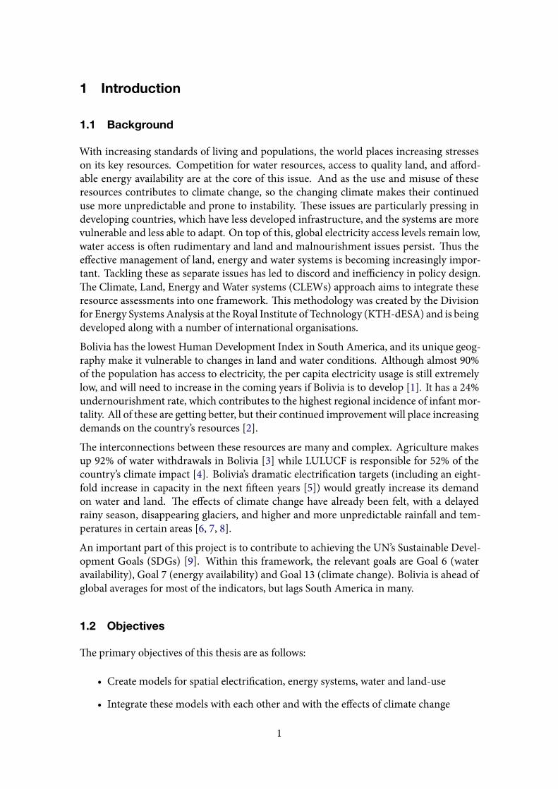
The primary objectives of this thesis are as follows:

• Create models for spatial electrification, energy systems, water and land-use

• Integrate these models with each other and with the effects of climate change

1

• Determine the pressure points between resources

Additionally, some extra objectives are included that do not form a core part of the discus-sion of this thesis, but are contributions to the work being carried out by KTH-dESA:

• Improve the ONSSET methodology and create a Python implementation of it

• Conduct testing and help with improvements on the Momani interface for OSe-MOSYS

2 The CLEWs nexus in Bolivia

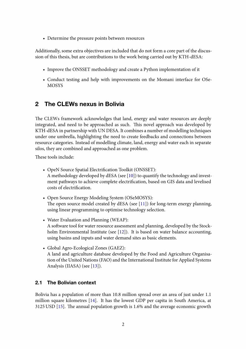
The CLEWs framework acknowledges that land, energy and water resources are deeplyintegrated, and need to be approached as such. This novel approach was developed byKTH-dESA in partnership with UNDESA. It combines a number of modelling techniquesunder one umbrella, highlighting the need to create feedbacks and connections betweenresource categories. Instead of modelling climate, land, energy and water each in separatesilos, they are combined and approached as one problem.

These tools include:

• OpeN Source Spatial Electrification Toolkit (ONSSET):A methodology developed by dESA (see [10]) to quantify the technology and invest-ment pathways to achieve complete electrification, based on GIS data and levelisedcosts of electrification.

• Open Source Energy Modeling System (OSeMOSYS):The open source model created by dESA (see [11]) for long-term energy planning,using linear programming to optimise technology selection.

• Water Evaluation and Planning (WEAP):A software tool for water resource assessment and planning, developed by the Stock-holm Environmental Institute (see [12]). It is based on water balance accounting,using basins and inputs and water demand sites as basic elements.

• Global Agro-Ecological Zones (GAEZ):A land and agriculture database developed by the Food and Agriculture Organisa-tion of the United Nations (FAO) and the International Institute for Applied SystemsAnalysis (IIASA) (see [13]).

2.1 The Bolivian context

Bolivia has a population of more than 10.8 million spread over an area of just under 1.1million square kilometres [14]. It has the lowest GDP per capita in South America, at3125USD [15]. The annual population growth is 1.6% and the average economic growth

2

for the last ten years was 4.9% [15]. The urbanised population in 2030 is expected to in-crease from the current 68.1% to 75.2% [16].

It is a landlocked country with a unique and varied geography. There are three broadlydefined geographic zones: the high-altitude Altiplano in the west, the humid slopes of theYungas valleys, and the temperate to tropical lowlands in the east and north. Each of theseareas has a drastically different climate, with additional variations within each zone. Eacharea has different challenges, along with different potentials for farming, energy and water.

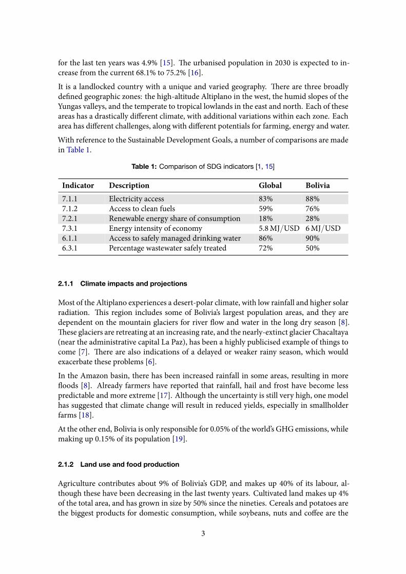
With reference to the Sustainable Development Goals, a number of comparisons are madein Table 1.

Table 1: Comparison of SDG indicators [1, 15]

Indicator Description Global Bolivia7.1.1 Electricity access 83% 88%7.1.2 Access to clean fuels 59% 76%7.2.1 Renewable energy share of consumption 18% 28%7.3.1 Energy intensity of economy 5.8MJ/USD 6MJ/USD6.1.1 Access to safely managed drinking water 86% 90%6.3.1 Percentage wastewater safely treated 72% 50%

2.1.1 Climate impacts and projections

Most of the Altiplano experiences a desert-polar climate, with low rainfall and higher solarradiation. This region includes some of Bolivia’s largest population areas, and they aredependent on the mountain glaciers for river flow and water in the long dry season [8].These glaciers are retreating at an increasing rate, and the nearly-extinct glacier Chacaltaya(near the administrative capital La Paz), has been a highly publicised example of things tocome [7]. There are also indications of a delayed or weaker rainy season, which wouldexacerbate these problems [6].

In the Amazon basin, there has been increased rainfall in some areas, resulting in morefloods [8]. Already farmers have reported that rainfall, hail and frost have become lesspredictable and more extreme [17]. Although the uncertainty is still very high, one modelhas suggested that climate change will result in reduced yields, especially in smallholderfarms [18].

At the other end, Bolivia is only responsible for 0.05% of the world’s GHG emissions, whilemaking up 0.15% of its population [19].

2.1.2 Land use and food production

Agriculture contributes about 9% of Bolivia’s GDP, and makes up 40% of its labour, al-though these have been decreasing in the last twenty years. Cultivated land makes up 4%of the total area, and has grown in size by 50% since the nineties. Cereals and potatoes arethe biggest products for domestic consumption, while soybeans, nuts and coffee are the

3

most important exports [2]. Forest cover has been decreasing by about half a percent peryear over the past twenty years.

The majority of the large, commercial farms are in the eastern lowlands, and have access tomodern technology and mechanisation, improved irrigation, and financing sources. How-ever, 94%of the agricultural units in the country belong to smallholder producers ofmostlystaple crops. Most of these are around the high Altiplano and Yungas valleys. These landparcels are family-ownedminifundios— sometimes as small as 500m2 — which are facinghigher demands and diminishing yields [20]. According to the Ministry of Rural Develop-ment and Land, 89% of the municipalities are classified with medium to high vulnerabilityto food insecurity [21].

2.1.3 The energy system

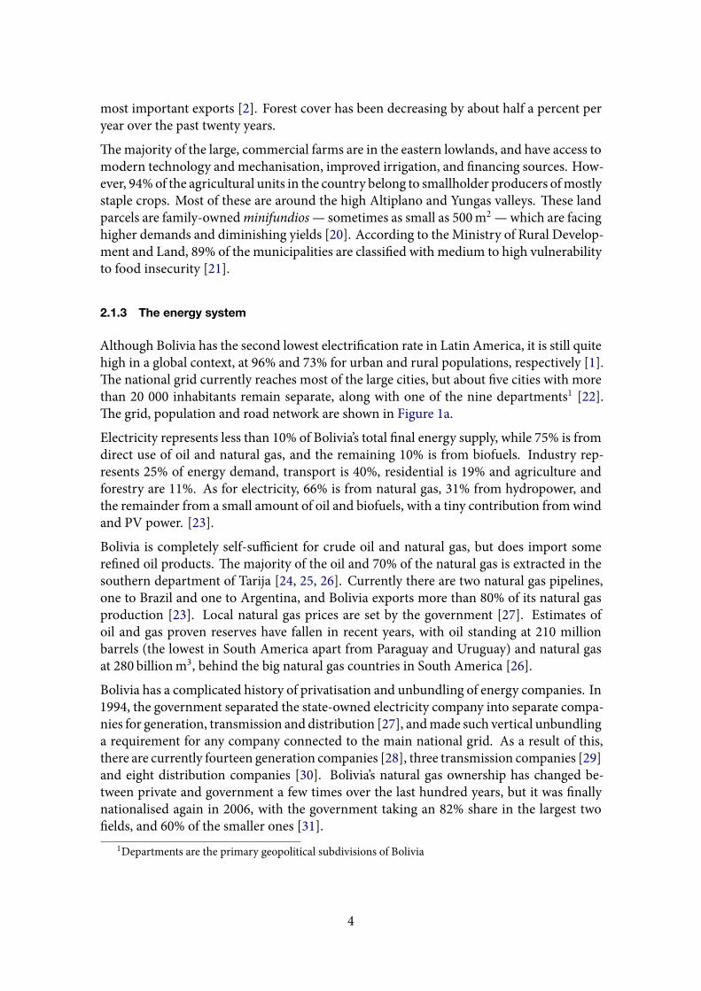
Although Bolivia has the second lowest electrification rate in Latin America, it is still quitehigh in a global context, at 96% and 73% for urban and rural populations, respectively [1].The national grid currently reaches most of the large cities, but about five cities with morethan 20 000 inhabitants remain separate, along with one of the nine departments1 [22].The grid, population and road network are shown in Figure 1a.

Electricity represents less than 10% of Bolivia’s total final energy supply, while 75% is fromdirect use of oil and natural gas, and the remaining 10% is from biofuels. Industry rep-resents 25% of energy demand, transport is 40%, residential is 19% and agriculture andforestry are 11%. As for electricity, 66% is from natural gas, 31% from hydropower, andthe remainder from a small amount of oil and biofuels, with a tiny contribution from windand PV power. [23].

Bolivia is completely self-sufficient for crude oil and natural gas, but does import somerefined oil products. The majority of the oil and 70% of the natural gas is extracted in thesouthern department of Tarija [24, 25, 26]. Currently there are two natural gas pipelines,one to Brazil and one to Argentina, and Bolivia exports more than 80% of its natural gasproduction [23]. Local natural gas prices are set by the government [27]. Estimates ofoil and gas proven reserves have fallen in recent years, with oil standing at 210 millionbarrels (the lowest in South America apart from Paraguay and Uruguay) and natural gasat 280 billionm3, behind the big natural gas countries in South America [26].

Bolivia has a complicated history of privatisation and unbundling of energy companies. In1994, the government separated the state-owned electricity company into separate compa-nies for generation, transmission and distribution [27], andmade such vertical unbundlinga requirement for any company connected to the main national grid. As a result of this,there are currently fourteen generation companies [28], three transmission companies [29]and eight distribution companies [30]. Bolivia’s natural gas ownership has changed be-tween private and government a few times over the last hundred years, but it was finallynationalised again in 2006, with the government taking an 82% share in the largest twofields, and 60% of the smaller ones [31].

1Departments are the primary geopolitical subdivisions of Bolivia

4

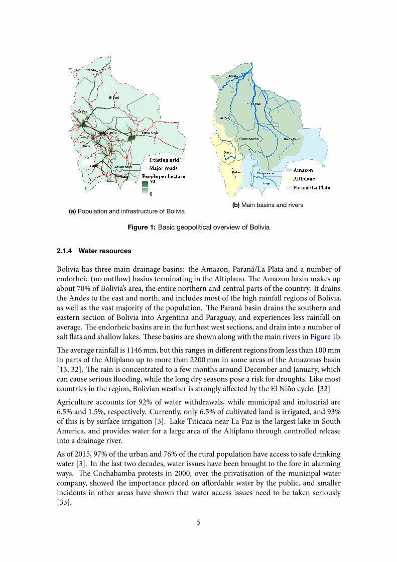
(a) Population and infrastructure of Bolivia(b) Main basins and rivers

Figure 1: Basic geopolitical overview of Bolivia

2.1.4 Water resources

Bolivia has three main drainage basins: the Amazon, Paraná/La Plata and a number ofendorheic (no outflow) basins terminating in the Altiplano. The Amazon basin makes upabout 70% of Bolivia’s area, the entire northern and central parts of the country. It drainsthe Andes to the east and north, and includes most of the high rainfall regions of Bolivia,as well as the vast majority of the population. The Paraná basin drains the southern andeastern section of Bolivia into Argentina and Paraguay, and experiences less rainfall onaverage. The endorheic basins are in the furthest west sections, and drain into a number ofsalt flats and shallow lakes. These basins are shown along with the main rivers in Figure 1b.The average rainfall is 1146mm, but this ranges in different regions from less than 100mmin parts of the Altiplano up to more than 2200mm in some areas of the Amazonas basin[13, 32]. The rain is concentrated to a few months around December and January, whichcan cause serious flooding, while the long dry seasons pose a risk for droughts. Like mostcountries in the region, Bolivian weather is strongly affected by the El Niño cycle. [32]Agriculture accounts for 92% of water withdrawals, while municipal and industrial are6.5% and 1.5%, respectively. Currently, only 6.5% of cultivated land is irrigated, and 93%of this is by surface irrigation [3]. Lake Titicaca near La Paz is the largest lake in SouthAmerica, and provides water for a large area of the Altiplano through controlled releaseinto a drainage river.As of 2015, 97% of the urban and 76% of the rural population have access to safe drinkingwater [3]. In the last two decades, water issues have been brought to the fore in alarmingways. The Cochabamba protests in 2000, over the privatisation of the municipal watercompany, showed the importance placed on affordable water by the public, and smallerincidents in other areas have shown that water access issues need to be taken seriously[33].

5

3 Methodology

3.1 Overview

The primary steps are as follows:

• Conduct a continuous literature study, to find indicators for pressure points, govern-ment plans and policies, critical issues in Bolivia and existing models.

• Collect andmanage data for climate, land, energy andwater throughonline databasesand Bolivian government as required. This needs to be organised and managed tomake it useable in the various tools.

• Create models for the various parts of the nexus, apply feedback and interactionswhere appropriate, and create scenarios.

• Combine quantitative modelling outputs with qualitative research outputs to drawconclusions and recommendations for Bolivian policy makers.

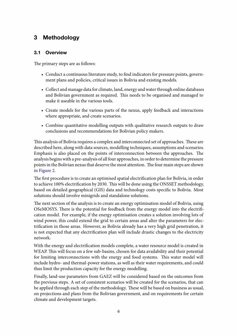
This analysis of Bolivia requires a complex and interconnected set of approaches. These aredescribed here, along with data sources, modelling techniques, assumptions and scenarios.Emphasis is also placed on the points of interconnection between the approaches. Theanalysis beginswith a pre-analysis of all four approaches, in order to determine the pressurepoints in the Bolivian nexus that deserve themost attention. The fourmain steps are shownin Figure 2.The first procedure is to create an optimised spatial electrification plan for Bolivia, in orderto achieve 100% electrification by 2030. This will be done using the ONSSETmethodology,based on detailed geographical (GIS) data and technology costs specific to Bolivia. Mostsolutions should involve minigrids and standalone solutions.The next section of the analysis is to create an energy optimisation model of Bolivia, usingOSeMOSYS. There is the potential for feedback from the energy model into the electrifi-cation model. For example, if the energy optimisation creates a solution involving lots ofwind power, this could extend the grid to certain areas and alter the parameters for elec-trification in those areas. However, as Bolivia already has a very high grid penetration, itis not expected that any electrification plan will include drastic changes to the electricitynetwork.With the energy and electrification models complete, a water resource model is created inWEAP. This will focus on a few sub-basins, chosen for data availability and their potentialfor limiting interconnections with the energy and food systems. This water model willinclude hydro- and thermal-power stations, as well as their water requirements, and couldthus limit the production capacity for the energy modelling.Finally, land-use parameters from GAEZ will be considered based on the outcomes fromthe previous steps. A set of consistent scenarios will be created for the scenarios, that canbe applied through each step of the methodology. These will be based on business as usual,on projections and plans from the Bolivian government, and on requirements for certainclimate and development targets.

6

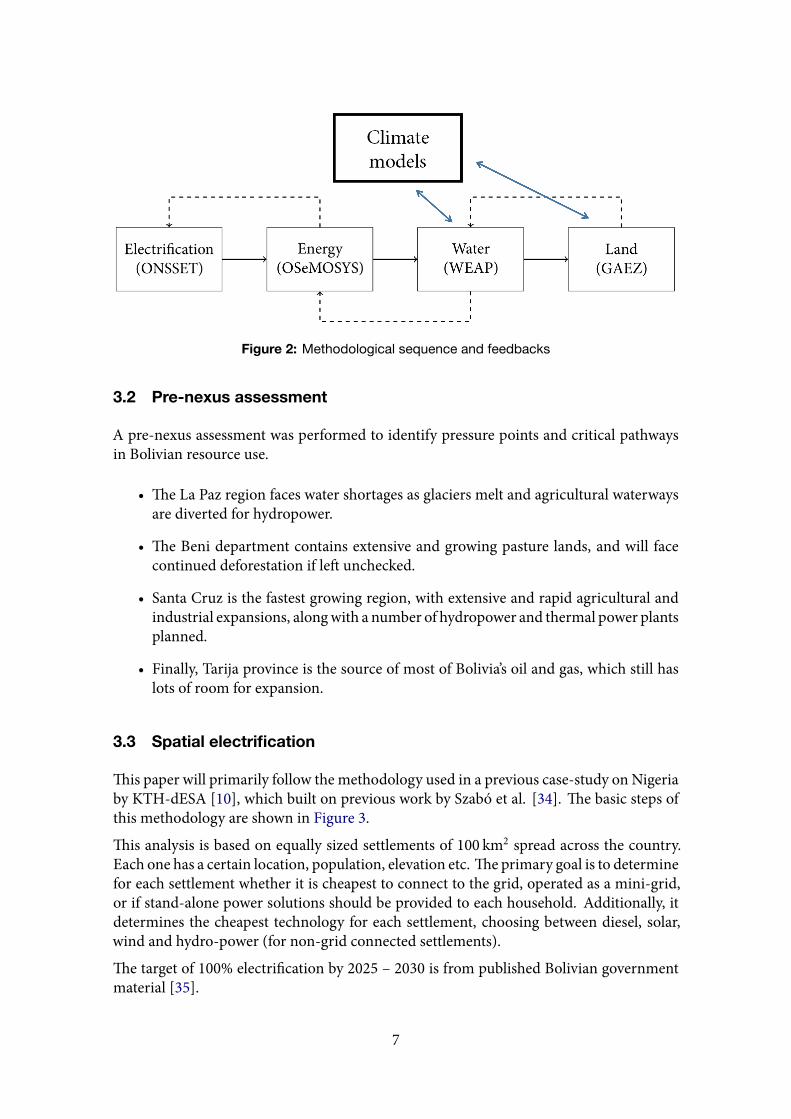
Figure 2: Methodological sequence and feedbacks

3.2 Pre-nexus assessment

A pre-nexus assessment was performed to identify pressure points and critical pathwaysin Bolivian resource use.

• The La Paz region faces water shortages as glaciers melt and agricultural waterwaysare diverted for hydropower.

• The Beni department contains extensive and growing pasture lands, and will facecontinued deforestation if left unchecked.

• Santa Cruz is the fastest growing region, with extensive and rapid agricultural andindustrial expansions, alongwith a number of hydropower and thermal power plantsplanned.

• Finally, Tarija province is the source of most of Bolivia’s oil and gas, which still haslots of room for expansion.

3.3 Spatial electrification

This paper will primarily follow the methodology used in a previous case-study on Nigeriaby KTH-dESA [10], which built on previous work by Szabó et al. [34]. The basic steps ofthis methodology are shown in Figure 3.

This analysis is based on equally sized settlements of 100 km2 spread across the country.Each one has a certain location, population, elevation etc. The primary goal is to determinefor each settlement whether it is cheapest to connect to the grid, operated as a mini-grid,or if stand-alone power solutions should be provided to each household. Additionally, itdetermines the cheapest technology for each settlement, choosing between diesel, solar,wind and hydro-power (for non-grid connected settlements).

The target of 100% electrification by 2025 – 2030 is from published Bolivian governmentmaterial [35].

7

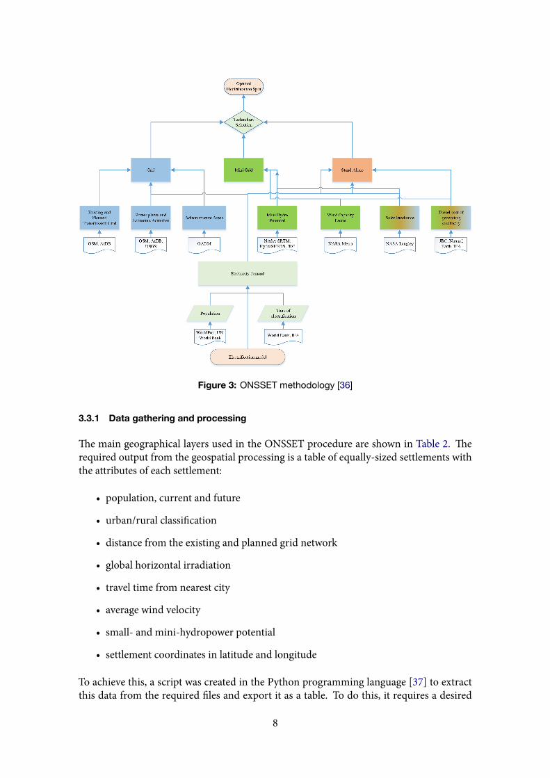
Figure 3: ONSSET methodology [36]

3.3.1 Data gathering and processing

The main geographical layers used in the ONSSET procedure are shown in Table 2. Therequired output from the geospatial processing is a table of equally-sized settlements withthe attributes of each settlement:

• population, current and future

• urban/rural classification

• distance from the existing and planned grid network

• global horizontal irradiation

• travel time from nearest city

• average wind velocity

• small- and mini-hydropower potential

• settlement coordinates in latitude and longitude

To achieve this, a script was created in the Python programming language [37] to extractthis data from the required files and export it as a table. To do this, it requires a desired

8

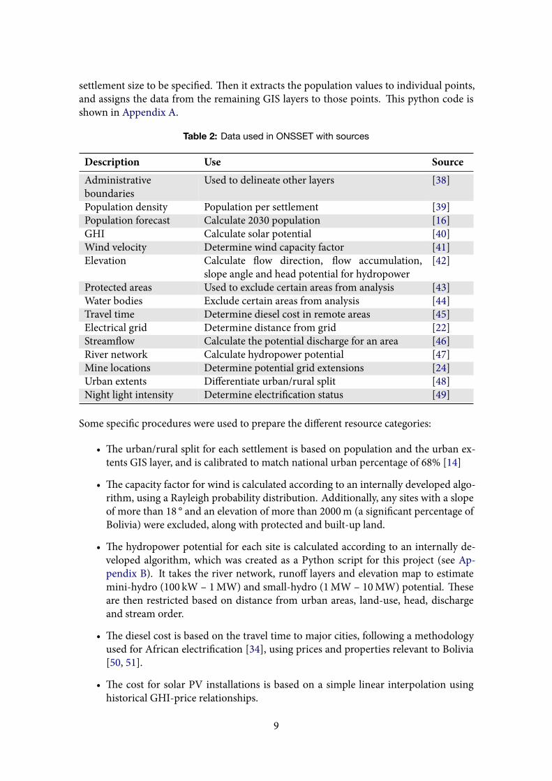
settlement size to be specified. Then it extracts the population values to individual points,and assigns the data from the remaining GIS layers to those points. This python code isshown in Appendix A.

Table 2: Data used in ONSSET with sources

Description Use SourceAdministrativeboundaries

Used to delineate other layers [38]

Population density Population per settlement [39]Population forecast Calculate 2030 population [16]GHI Calculate solar potential [40]Wind velocity Determine wind capacity factor [41]Elevation Calculate flow direction, flow accumulation,

slope angle and head potential for hydropower[42]

Protected areas Used to exclude certain areas from analysis [43]Water bodies Exclude certain areas from analysis [44]Travel time Determine diesel cost in remote areas [45]Electrical grid Determine distance from grid [22]Streamflow Calculate the potential discharge for an area [46]River network Calculate hydropower potential [47]Mine locations Determine potential grid extensions [24]Urban extents Differentiate urban/rural split [48]Night light intensity Determine electrification status [49]

Some specific procedures were used to prepare the different resource categories:

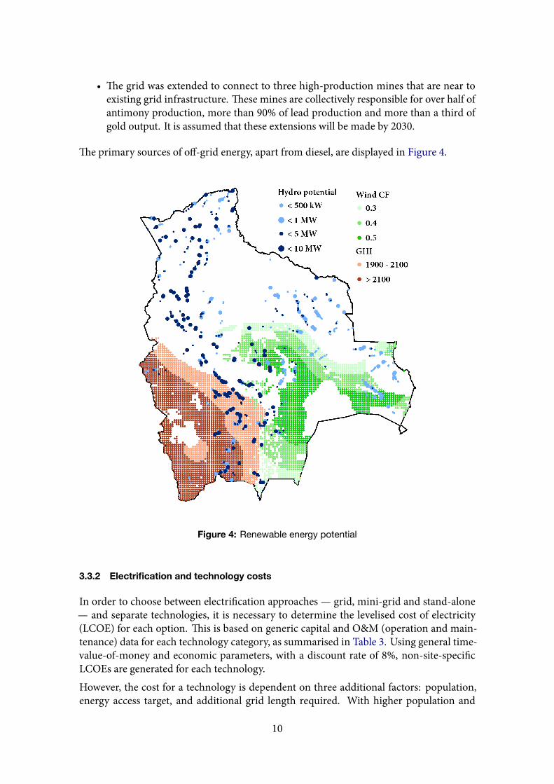
• The urban/rural split for each settlement is based on population and the urban ex-tents GIS layer, and is calibrated to match national urban percentage of 68% [14]

• The capacity factor for wind is calculated according to an internally developed algo-rithm, using a Rayleigh probability distribution. Additionally, any sites with a slopeof more than 18 ° and an elevation of more than 2000m (a significant percentage ofBolivia) were excluded, along with protected and built-up land.

• The hydropower potential for each site is calculated according to an internally de-veloped algorithm, which was created as a Python script for this project (see Ap-pendix B). It takes the river network, runoff layers and elevation map to estimatemini-hydro (100 kW – 1MW) and small-hydro (1MW – 10MW) potential. Theseare then restricted based on distance from urban areas, land-use, head, dischargeand stream order.

• The diesel cost is based on the travel time to major cities, following a methodologyused for African electrification [34], using prices and properties relevant to Bolivia[50, 51].

• The cost for solar PV installations is based on a simple linear interpolation usinghistorical GHI-price relationships.

9

• The grid was extended to connect to three high-production mines that are near toexisting grid infrastructure. These mines are collectively responsible for over half ofantimony production, more than 90% of lead production and more than a third ofgold output. It is assumed that these extensions will be made by 2030.

The primary sources of off-grid energy, apart from diesel, are displayed in Figure 4.

Figure 4: Renewable energy potential

3.3.2 Electrification and technology costs

In order to choose between electrification approaches — grid, mini-grid and stand-alone— and separate technologies, it is necessary to determine the levelised cost of electricity(LCOE) for each option. This is based on generic capital and O&M (operation and main-tenance) data for each technology category, as summarised in Table 3. Using general time-value-of-money and economic parameters, with a discount rate of 8%, non-site-specificLCOEs are generated for each technology.However, the cost for a technology is dependent on three additional factors: population,energy access target, and additional grid length required. With higher population and

10

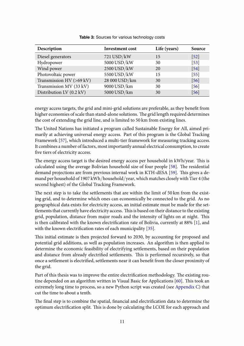
Table 3: Sources for various technology costs

Description Investment cost Life (years) SourceDiesel generators 721USD/kW 15 [52]Hydropower 5000USD/kW 30 [53]Wind power 2500USD/kW 20 [54]Photovoltaic power 5500USD/kW 15 [55]Transmission HV (>69 kV) 28 000USD/km 30 [56]Transmission MV (33 kV) 9000USD/km 30 [56]Distribution LV (0.2 kV) 5000USD/km 30 [56]

energy access targets, the grid and mini-grid solutions are preferable, as they benefit fromhigher economies of scale than stand-alone solutions. The grid length required determinesthe cost of extending the grid line, and is limited to 50 km from existing lines.

The United Nations has initiated a program called Sustainable Energy for All, aimed pri-marily at achieving universal energy access. Part of this program is the Global TrackingFramework [57], which introduced a multi-tier framework for measuring tracking access.It combines a number of factors, most importantly annual electrical consumption, to createfive tiers of electricity access.

The energy access target is the desired energy access per household in kWh/year. This iscalculated using the average Bolivian household size of four people [58]. The residentialdemand projections are from previous internal work in KTH-dESA [59]. This gives a de-mand per household of 1907 kWh/household/year, whichmatches closely with Tier 4 (thesecond highest) of the Global Tracking Framework.

The next step is to take the settlements that are within the limit of 50 km from the exist-ing grid, and to determine which ones can economically be connected to the grid. As nogeographical data exists for electricity access, an initial estimate must be made for the set-tlements that currently have electricity access. This is based on their distance to the existinggrid, population, distance from major roads and the intensity of lights on at night. Thisis then calibrated with the known electrification rate of Bolivia, currently at 88% [1], andwith the known electrification rates of each municipality [35].

This initial estimate is then projected forward to 2030, by accounting for proposed andpotential grid additions, as well as population increases. An algorithm is then applied todetermine the economic feasibility of electrifying settlements, based on their populationand distance from already electrified settlements. This is performed recursively, so thatonce a settlement is electrified, settlements near it can benefit from the closer proximity ofthe grid.

Part of this thesis was to improve the entire electrification methodology. The existing rou-tine depended on an algorithm written in Visual Basic for Applications [60]. This took anextremely long time to process, so a new Python script was created (see Appendix C) thatcut the time to about a tenth.

The final step is to combine the spatial, financial and electrification data to determine theoptimum electrification split. This is done by calculating the LCOE for each approach and

11

technology, and then choosing the cheapest option for each site. A separate investmentcost is also calculated, which is the total capital expenditure for each site.

3.4 Energy system optimisation

The next step in the CLEWs framework is to use OSeMOSYS to determine the optimumenergy mix for the grid connected generation. This model uses the GLPK (GNU LinearProgramming Kit) to find the optimal mix, based on technologies and fuels entered by theuser. For this project, the Model Management Interface (MoManI) will be used to createthe models. This is a web interface that is being created within KTH-dESA to make usingthe OSeMOSYS modelling technique much easier and available to anyone with an internetconnection.

The purpose of this model is to determine the optimum energy system investments un-til the year 2040. Of particular interest is the interconnections with water usage. Thusthe primary stages of the system (fuel extraction and refining) are modelled very simply,with more emphasis placed on accurately capturing temporal characteristics, especially forwater-intensive thermal- and hydro-power generation. The range of technologies is alsorestricted, with unlikely technologies excluded from the mix (notably nuclear and coalpower, as Bolivia has no concrete nuclear plans, and no significant coal reserves).

Finally, the model was limited to grid-connected production and demand, as it is assumedthat the previous electrification methodology will handle the off-grid characterisation bet-ter.

3.4.1 Reference energy system

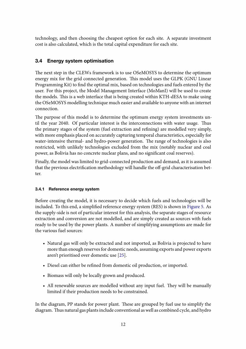
Before creating the model, it is necessary to decide which fuels and technologies will beincluded. To this end, a simplified reference energy system (RES) is shown in Figure 5. Asthe supply-side is not of particular interest for this analysis, the separate stages of resourceextraction and conversion are not modelled, and are simply created as sources with fuelsready to be used by the power plants. A number of simplifying assumptions are made forthe various fuel sources:

• Natural gas will only be extracted and not imported, as Bolivia is projected to havemore than enough reserves for domestic needs, assuming exports and power exportsaren’t prioritised over domestic use [25].

• Diesel can either be refined from domestic oil production, or imported.

• Biomass will only be locally grown and produced.

• All renewable sources are modelled without any input fuel. They will be manuallylimited if their production needs to be constrained.

In the diagram, PP stands for power plant. These are grouped by fuel use to simplify thediagram. Thusnatural gas plants include conventional aswell as combined cycle, andhydro

12

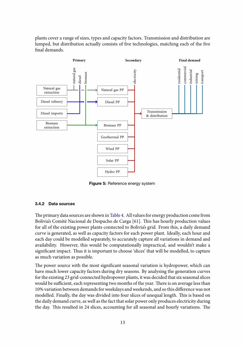
plants cover a range of sizes, types and capacity factors. Transmission and distribution arelumped, but distribution actually consists of five technologies, matching each of the fivefinal demands.

Natural gasextraction

Diesel refinery

Diesel imports

Biomassextraction

natu

ralg

asdi

esel

biom

ass

Natural gas PP

Diesel PP

Biomass PP

Geothermal PP

Wind PP

Solar PP

Hydro PP

Transmission& distribution

elec

tricity

resid

entia

lco

mm

ercial

indu

strial

min

ing

tran

spor

t

Primary Secondary Final demand

Figure 5: Reference energy system

3.4.2 Data sources

Theprimary data sources are shown inTable 4. All values for energy production come fromBolivia’s Comité Nacional de Despacho de Carga [61]. This has hourly production valuesfor all of the existing power plants connected to Bolivia’s grid. From this, a daily demandcurve is generated, as well as capacity factors for each power plant. Ideally, each hour andeach day could be modelled separately, to accurately capture all variations in demand andavailability. However, this would be computationally impractical, and wouldn’t make asignificant impact. Thus it is important to choose ‘slices’ that will be modelled, to captureas much variation as possible.

The power source with the most significant seasonal variation is hydropower, which canhave much lower capacity factors during dry seasons. By analysing the generation curvesfor the existing 23 grid-connected hydropower plants, it was decided that six seasonal sliceswould be sufficient, each representing twomonths of the year. There is on average less than10%variation between demands forweekdays andweekends, and so this differencewas notmodelled. Finally, the day was divided into four slices of unequal length. This is based onthe daily demand curve, as well as the fact that solar power only produces electricity duringthe day. This resulted in 24 slices, accounting for all seasonal and hourly variations. The

13

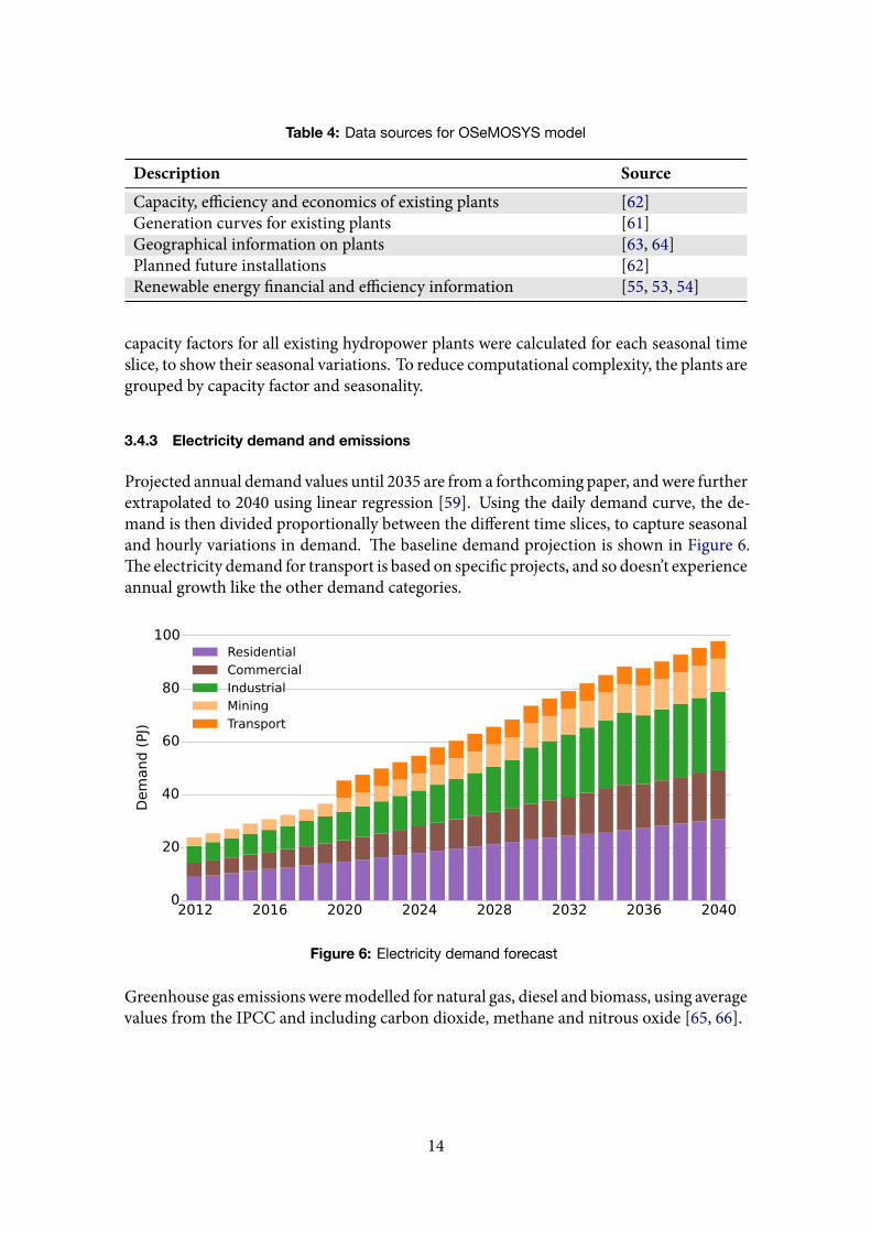
Table 4: Data sources for OSeMOSYS model

Description SourceCapacity, efficiency and economics of existing plants [62]Generation curves for existing plants [61]Geographical information on plants [63, 64]Planned future installations [62]Renewable energy financial and efficiency information [55, 53, 54]

capacity factors for all existing hydropower plants were calculated for each seasonal timeslice, to show their seasonal variations. To reduce computational complexity, the plants aregrouped by capacity factor and seasonality.

3.4.3 Electricity demand and emissions

Projected annual demand values until 2035 are from a forthcoming paper, andwere furtherextrapolated to 2040 using linear regression [59]. Using the daily demand curve, the de-mand is then divided proportionally between the different time slices, to capture seasonaland hourly variations in demand. The baseline demand projection is shown in Figure 6.The electricity demand for transport is based on specific projects, and so doesn’t experienceannual growth like the other demand categories.

2012 2016 2020 2024 2028 2032 2036 20400

20

40

60

80

100

Demand (PJ)

ResidentialCommercialIndustrialMiningTransport

Figure 6: Electricity demand forecast

Greenhouse gas emissionsweremodelled for natural gas, diesel and biomass, using averagevalues from the IPCC and including carbon dioxide, methane and nitrous oxide [65, 66].

14

3.5 Water resources and land use

The final component of this CLEWs analysis is to model a few key water basins, and todetermine how the water and land use is connected to the energy system already created.This is done using the WEAP water modelling system. This software is capable of highlydetailed analysis on specific water basins, including water quality and advanced runoff andevapotranspiration modelling. However, as this is geographically a very large model thatwill cover basins totalling 430 000 km2 (40% of Bolivia’s surface area, along with a smallpart of northern Argentina), a very simplified approach will be used.

The primary aim is to accurately capture the water potential and demands, and how thesewill impact or be impacted by energy and agricultural land-use expansions. With this goalit is not necessary to model in extremely fine detail, and large areas coveringmultiple citiescan bemodelled as single demand sites. Additionally, the modelling requires stream gaugedata for calibration, and the level of confidence possible is limited by this data availability.

3.5.1 Basin delineation

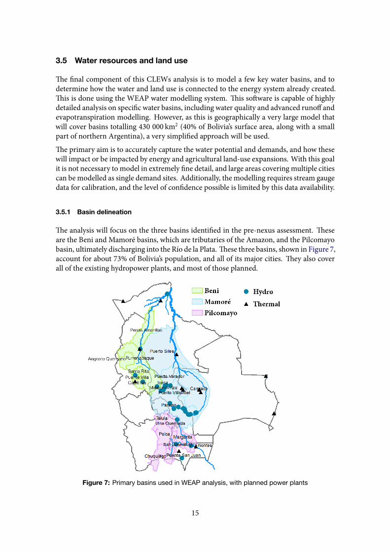
The analysis will focus on the three basins identified in the pre-nexus assessment. Theseare the Beni and Mamoré basins, which are tributaries of the Amazon, and the Pilcomayobasin, ultimately discharging into the Río de la Plata. These three basins, shown in Figure 7,account for about 73% of Bolivia’s population, and all of its major cities. They also coverall of the existing hydropower plants, and most of those planned.

Figure 7: Primary basins used in WEAP analysis, with planned power plants

15

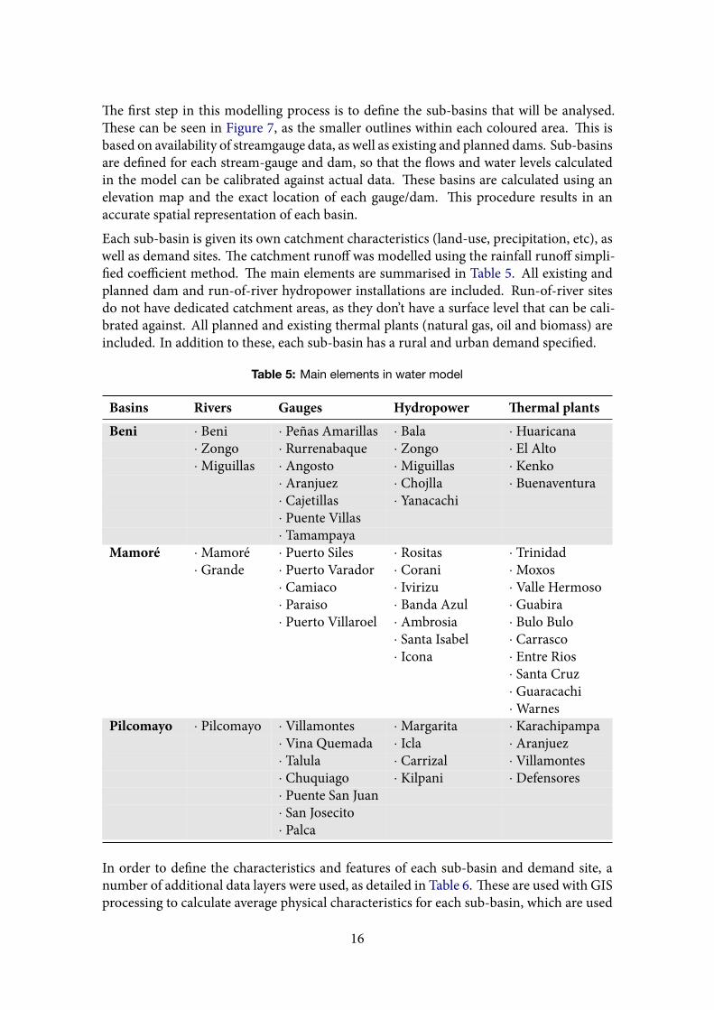
The first step in this modelling process is to define the sub-basins that will be analysed.These can be seen in Figure 7, as the smaller outlines within each coloured area. This isbased on availability of streamgauge data, as well as existing and planned dams. Sub-basinsare defined for each stream-gauge and dam, so that the flows and water levels calculatedin the model can be calibrated against actual data. These basins are calculated using anelevation map and the exact location of each gauge/dam. This procedure results in anaccurate spatial representation of each basin.Each sub-basin is given its own catchment characteristics (land-use, precipitation, etc), aswell as demand sites. The catchment runoff was modelled using the rainfall runoff simpli-fied coefficient method. The main elements are summarised in Table 5. All existing andplanned dam and run-of-river hydropower installations are included. Run-of-river sitesdo not have dedicated catchment areas, as they don’t have a surface level that can be cali-brated against. All planned and existing thermal plants (natural gas, oil and biomass) areincluded. In addition to these, each sub-basin has a rural and urban demand specified.

Table 5: Main elements in water model

Basins Rivers Gauges Hydropower Thermal plantsBeni · Beni · Peñas Amarillas · Bala · Huaricana

· Zongo · Rurrenabaque · Zongo · El Alto· Miguillas · Angosto · Miguillas · Kenko

· Aranjuez · Chojlla · Buenaventura· Cajetillas · Yanacachi· Puente Villas· Tamampaya

Mamoré · Mamoré · Puerto Siles · Rositas · Trinidad· Grande · Puerto Varador · Corani · Moxos

· Camiaco · Ivirizu · Valle Hermoso· Paraiso · Banda Azul · Guabira· Puerto Villaroel · Ambrosia · Bulo Bulo

· Santa Isabel · Carrasco· Icona · Entre Rios

· Santa Cruz· Guaracachi· Warnes

Pilcomayo · Pilcomayo · Villamontes · Margarita · Karachipampa· Vina Quemada · Icla · Aranjuez· Talula · Carrizal · Villamontes· Chuquiago · Kilpani · Defensores· Puente San Juan· San Josecito· Palca

In order to define the characteristics and features of each sub-basin and demand site, anumber of additional data layers were used, as detailed in Table 6. These are used with GISprocessing to calculate average physical characteristics for each sub-basin, which are used

16

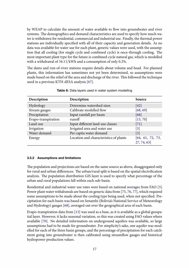
by WEAP to calculate the amount of water available to flow into groundwater and riversystems. The demographics and demand characteristics are used to specify how much wa-ter is withdrawn for residential, commercial and industrial use. Finally, the thermal powerstations are individually specified with all of their capacity and generation details. As nodata was available for water use for each plant, generic values were used, with the assump-tion that all cooling (for single cycle and combined cycle) is once-through cooling. Themost important plant type for the future is combined cycle natural gas, which is modelledwith a withdrawal of 34.1 l/kWh and a consumption of only 0.2%.

The dams and run-of-river stations require details about volume and head. For plannedplants, this information has sometimes not yet been determined, so assumptions weremade based on the relief of the area and discharge of the river. This followed the techniqueused in a previous KTH-dESA analysis [67].

Table 6: Data layers used in water system modelling

Description Description SourceHydrology Determine watershed sizes [42]Stream gauges Calibrate modelled flow [68, 69]Precipitation Input rainfall per basin [68]Evapo-transpiration runoff [13, 70]Land-use Input different land-use classes [71]Irrigation Irrigated area and water use [3]Water demand Per capita water demand [3]Energy Location and characteristics of plants [64, 61, 72, 73,

27, 74, 63]

3.5.2 Assumptions and limitations

The population and projections are based on the same source as above, disaggregated onlyfor rural and urban differences. The urban/rural split is based on the spatial electrificationanalysis. The population distribution GIS layer is used to specify what percentage of theurban and rural populations fall within each sub-basin.

Residential and industrial water use rates were based on national averages from FAO [3].Power plant water withdrawals are based on generic data from [75, 76, 77], which requiredsome assumptions to be made about the cooling type being used, when not specified. Pre-cipitation for each basin was based on Senamhi (Bolivia’s National Service of Meteorologyand Hydrology) gauges [68], averaged out over the geographical area of each basin.

Evapo-transpiration data from [13] was used as a base, as it is available as a global geospa-tial layer. However, it lacks seasonal variation, so this was created using FAO values whereavailable [70]. No detailed information on underground aquifers was available, so largeassumptions had to be made for groundwater. For simplicity’s sake, one aquifer was mod-elled for each of the three basin groups, and the percentage of precipitation for each catch-ment going into groundwater is then calibrated using streamflow gauges and historicalhydropower production values.

17

WEAP was setup using the rainfall runoff – simplified coefficient method. This method ofdetermining runoff from precipitation has the lowest data requirements, and was chosenas the most suitable method for a model covering such a large geographical area.

3.5.3 Catchments, land-use and demand sites

Due to data limitations, the level of detail in land-use modelling is quite limited. The land-use categories used were forest, general agriculture and irrigated land. There was no dataavailable for land-use and irrigation coverage for each area, so the national statistics wereused, along with assumptions based on low resolution geospatial land-use data [71]. Thenational FAO statistics [3] suggest that 0.3% of the Bolivia’s land area is currently irrigated(about 3000 km2). It is assumed that 90% of this irrigated land falls within the area of theanalysis (the remaining areas being mostly desert, forest or pasture), so that the averagebased on this smaller area then becomes 0.7% irrigated. This is applied to all the catchmentareas, as no better data is available. To include a more realistic projection in the model, a4% annual growth in irrigated area is added, resulting in a doubled irrigated area by 2030(compared to the INDC target of triple).

For the same reason, the actual land cover was limited to two categories: forest and grain.This impacts the evapotranspiration, which won’t be accurately captured by incorrect landuse. This will, however, be easier to rectify in the future with improved land-use data.

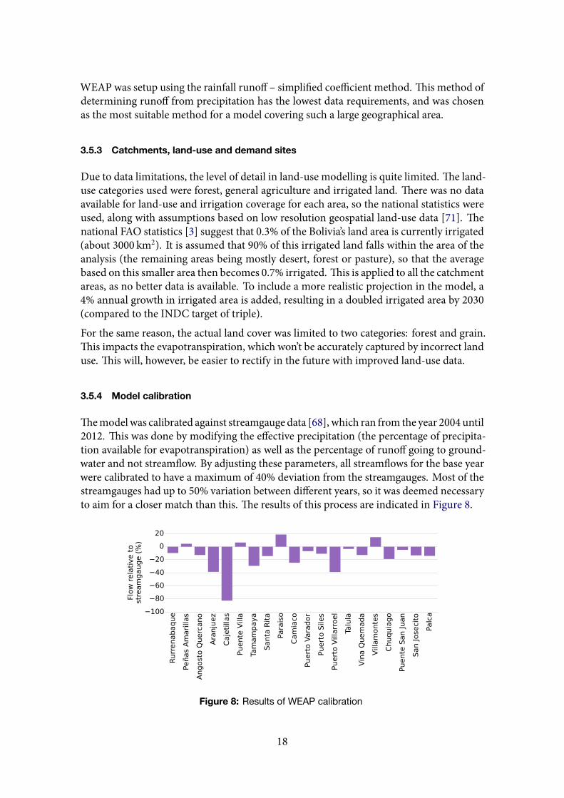
3.5.4 Model calibration

Themodelwas calibrated against streamgauge data [68], which ran from the year 2004 until2012. This was done by modifying the effective precipitation (the percentage of precipita-tion available for evapotranspiration) as well as the percentage of runoff going to ground-water and not streamflow. By adjusting these parameters, all streamflows for the base yearwere calibrated to have a maximum of 40% deviation from the streamgauges. Most of thestreamgauges had up to 50% variation between different years, so it was deemed necessaryto aim for a closer match than this. The results of this process are indicated in Figure 8.

Rurr

enabaque

Peñas

Am

ari

llas

Angost

o Q

uerc

ano

Ara

nju

ez

Caje

tilla

s

Puente

Vill

a

Tam

am

paya

Santa

Rit

a

Para

iso

Cam

iaco

Puert

o V

ara

dor

Puert

o S

iles

Puert

o V

illarr

oel

Talu

la

Vin

a Q

uem

ada

Vill

am

onte

s

Chuquia

go

Puente

San Juan

San Jose

cito

Palc

a−100

−80

−60

−40

−20

0

20

Flow

rela

tive t

o

stre

am

gauge (

%)

Figure 8: Results of WEAP calibration

18

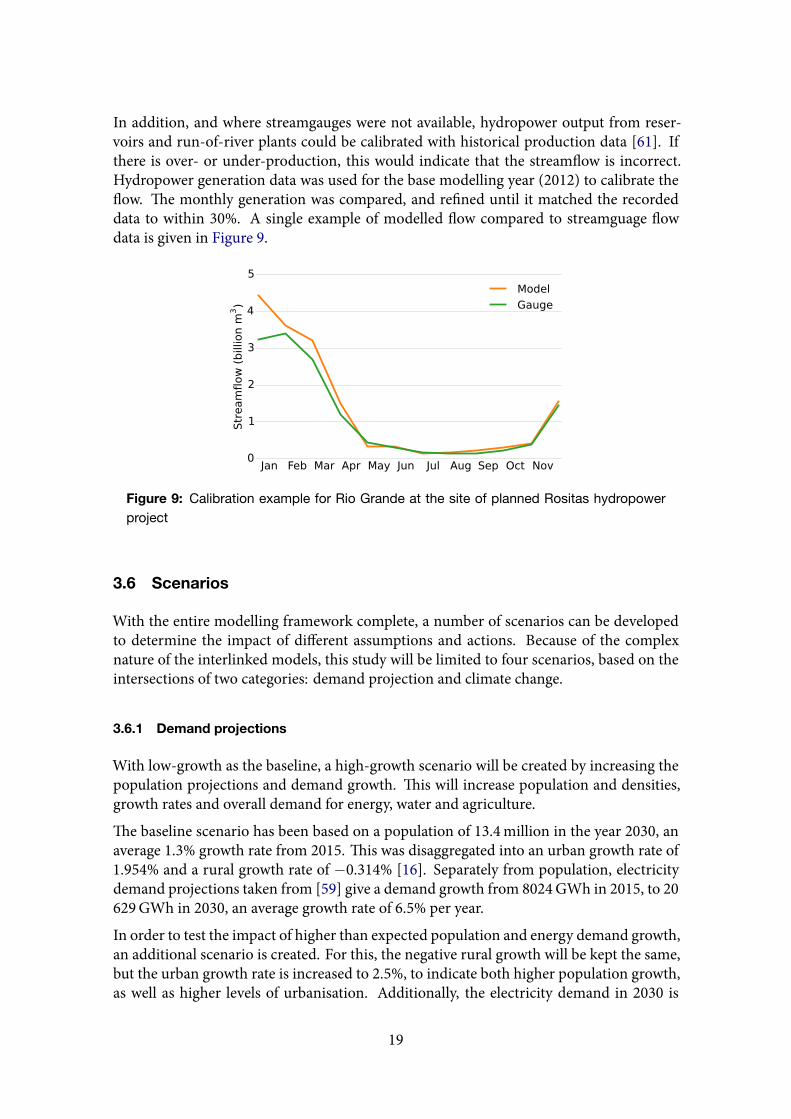
In addition, and where streamgauges were not available, hydropower output from reser-voirs and run-of-river plants could be calibrated with historical production data [61]. Ifthere is over- or under-production, this would indicate that the streamflow is incorrect.Hydropower generation data was used for the base modelling year (2012) to calibrate theflow. The monthly generation was compared, and refined until it matched the recordeddata to within 30%. A single example of modelled flow compared to streamguage flowdata is given in Figure 9.

Jan Feb Mar Apr May Jun Jul Aug Sep Oct Nov0

1

2

3

4

5

Streamflow (billion m

3)

Model

Gauge

Figure 9: Calibration example for Rio Grande at the site of planned Rositas hydropowerproject

3.6 Scenarios

With the entire modelling framework complete, a number of scenarios can be developedto determine the impact of different assumptions and actions. Because of the complexnature of the interlinked models, this study will be limited to four scenarios, based on theintersections of two categories: demand projection and climate change.

3.6.1 Demand projections

With low-growth as the baseline, a high-growth scenario will be created by increasing thepopulation projections and demand growth. This will increase population and densities,growth rates and overall demand for energy, water and agriculture.

The baseline scenario has been based on a population of 13.4million in the year 2030, anaverage 1.3% growth rate from 2015. This was disaggregated into an urban growth rate of1.954% and a rural growth rate of −0.314% [16]. Separately from population, electricitydemand projections taken from [59] give a demand growth from 8024GWh in 2015, to 20629GWh in 2030, an average growth rate of 6.5% per year.

In order to test the impact of higher than expected population and energy demand growth,an additional scenario is created. For this, the negative rural growth will be kept the same,but the urban growth rate is increased to 2.5%, to indicate both higher population growth,as well as higher levels of urbanisation. Additionally, the electricity demand in 2030 is

19

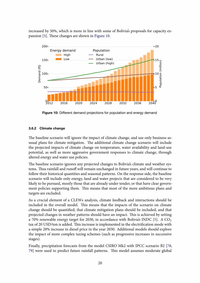
increased by 50%, which is more in line with some of Bolivia’s proposals for capacity ex-pansion [5]. These changes are shown in Figure 10.

2012 2016 2020 2024 2028 2032 2036 20400

50

100

150

200

Dem

and (PJ)

Energy demandHigh

Low

0

5

10

15

20

Popula

tion (m

illio

n)

PopulationRural

Urban (low)

Urban (high)

Figure 10: Different demand projections for population and energy demand

3.6.2 Climate change

The baseline scenario will ignore the impact of climate change, and use only business-as-usual plans for climate mitigation. The additional climate change scenario will includethe projected impacts of climate change on temperature, water availability and land-usepotential, as well as more aggressive government responses to climate change, throughaltered energy and water use policies.

The baseline scenario ignores any projected changes to Bolivia’s climate and weather sys-tems. Thus rainfall and runoff will remain unchanged in future years, and will continue tofollow their historical quantities and seasonal patterns. On the response side, the baselinescenario will include only energy, land and water projects that are considered to be verylikely to be pursued, mostly those that are already under tender, or that have clear govern-ment policies supporting them. This means that most of the more ambitious plans andtargets are excluded.

As a crucial element of a CLEWs analysis, climate feedback and interactions should beincluded in the overall model. This means that the impacts of the scenario on climatechange should be quantified, that climate mitigation plans should be included, and thatprojected changes in weather patterns should have an impact. This is achieved by settinga 70% renewable energy target for 2030, in accordance with Bolivia’s INDC [5]. A CO2tax of 20 USD/ton is added. This increase is implemented in the electrification mode witha simple 28% increase in diesel price in the year 2030. Additional models should explorethe impact of more complex taxing schemes (such as progressive increases in successivestages).

Finally, precipitation forecasts from the model CSIRO Mk2 with IPCC scenario B2 [78,79] were used to predict future rainfall patterns. This model assumes moderate global

20

Ara

nju

ez

Caje

tilla

s

Zongo

Puente

Vill

a

Mig

uill

as

Tam

am

paya

Santa

Rit

a

Angost

o Q

uerc

ano

Rurr

enabaque

Mis

icuni

Peñas

Am

ari

llas

Para

iso

Cam

iaco

Puert

o V

illarr

oel

Ivir

izu

Cora

ni

Icona

Puert

o V

ara

dor

Puert

o S

iles

Talu

la

Palc

a

Vin

a Q

uem

ada

Chuquia

go

Puente

San Juan

San Jose

cito

Puest

o M

arg

ari

ta

Vill

am

onte

s−40

−30

−20

−10

0

10

20

30

Perc

enta

ge c

hange

Beni Mamore Pilcomayo

2020s

2050s

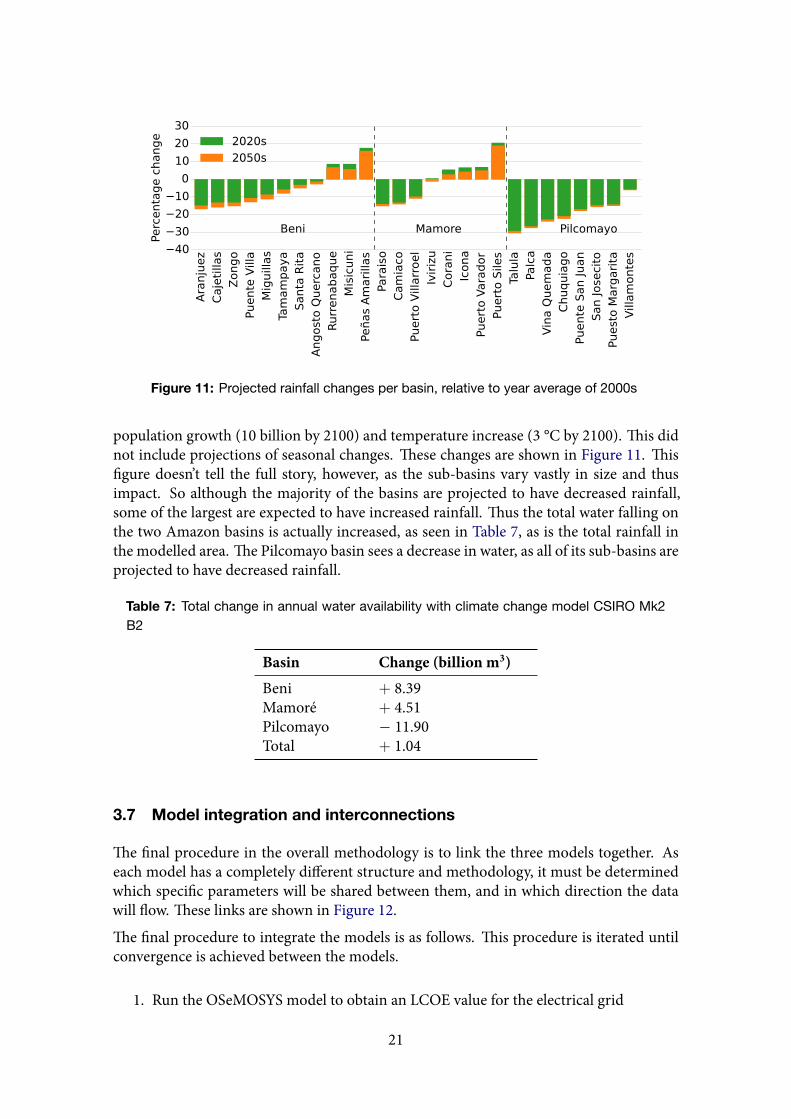
Figure 11: Projected rainfall changes per basin, relative to year average of 2000s

population growth (10 billion by 2100) and temperature increase (3 °C by 2100). This didnot include projections of seasonal changes. These changes are shown in Figure 11. Thisfigure doesn’t tell the full story, however, as the sub-basins vary vastly in size and thusimpact. So although the majority of the basins are projected to have decreased rainfall,some of the largest are expected to have increased rainfall. Thus the total water falling onthe two Amazon basins is actually increased, as seen in Table 7, as is the total rainfall inthe modelled area. The Pilcomayo basin sees a decrease in water, as all of its sub-basins areprojected to have decreased rainfall.

Table 7: Total change in annual water availability with climate change model CSIRO Mk2B2

Basin Change (billion m3)Beni + 8.39Mamoré + 4.51Pilcomayo − 11.90Total + 1.04

3.7 Model integration and interconnections

The final procedure in the overall methodology is to link the three models together. Aseach model has a completely different structure and methodology, it must be determinedwhich specific parameters will be shared between them, and in which direction the datawill flow. These links are shown in Figure 12.

The final procedure to integrate the models is as follows. This procedure is iterated untilconvergence is achieved between the models.

1. Run the OSeMOSYS model to obtain an LCOE value for the electrical grid

21

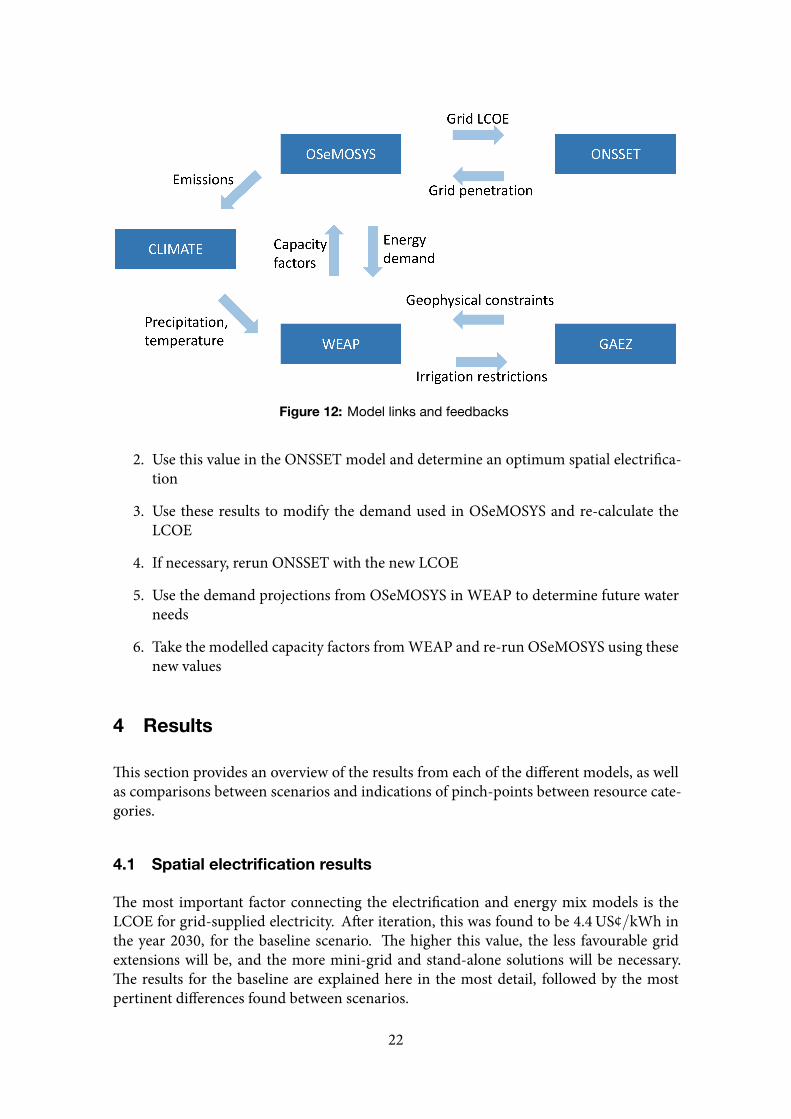
Figure 12: Model links and feedbacks

2. Use this value in the ONSSET model and determine an optimum spatial electrifica-tion

3. Use these results to modify the demand used in OSeMOSYS and re-calculate theLCOE

4. If necessary, rerun ONSSET with the new LCOE

5. Use the demand projections from OSeMOSYS in WEAP to determine future waterneeds

6. Take the modelled capacity factors from WEAP and re-run OSeMOSYS using thesenew values

4 Results

This section provides an overview of the results from each of the different models, as wellas comparisons between scenarios and indications of pinch-points between resource cate-gories.

4.1 Spatial electrification results

The most important factor connecting the electrification and energy mix models is theLCOE for grid-supplied electricity. After iteration, this was found to be 4.4US¢/kWh inthe year 2030, for the baseline scenario. The higher this value, the less favourable gridextensions will be, and the more mini-grid and stand-alone solutions will be necessary.The results for the baseline are explained here in the most detail, followed by the mostpertinent differences found between scenarios.

22

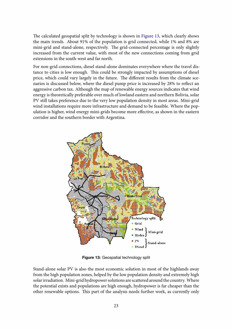
The calculated geospatial split by technology is shown in Figure 13, which clearly showsthe main trends. About 91% of the population is grid connected, while 1% and 8% aremini-grid and stand-alone, respectively. The grid-connected percentage is only slightlyincreased from the current value, with most of the new connections coming from gridextensions in the south-west and far north.

For non-grid connections, diesel stand-alone dominates everywhere where the travel dis-tance to cities is low enough. This could be strongly impacted by assumptions of dieselprice, which could vary largely in the future. The different results from the climate sce-narios is discussed below, where the diesel pump price is increased by 28% to reflect anaggressive carbon tax. Although the map of renewable energy sources indicates that windenergy is theoretically preferable over much of lowland eastern and northern Bolivia, solarPV still takes preference due to the very low population density in most areas. Mini-gridwind installations require more infrastructure and demand to be feasible. Where the pop-ulation is higher, wind energy mini-grids become more effective, as shown in the easterncorridor and the southern border with Argentina.

Figure 13: Geospatial technology split

Stand-alone solar PV is also the most economic solution in most of the highlands awayfrom the high population zones, helped by the low population density and extremely highsolar irradiation. Mini-grid hydropower solutions are scattered around the country. Wherethe potential exists and populations are high enough, hydropower is far cheaper than theother renewable options. This part of the analysis needs further work, as currently only

23

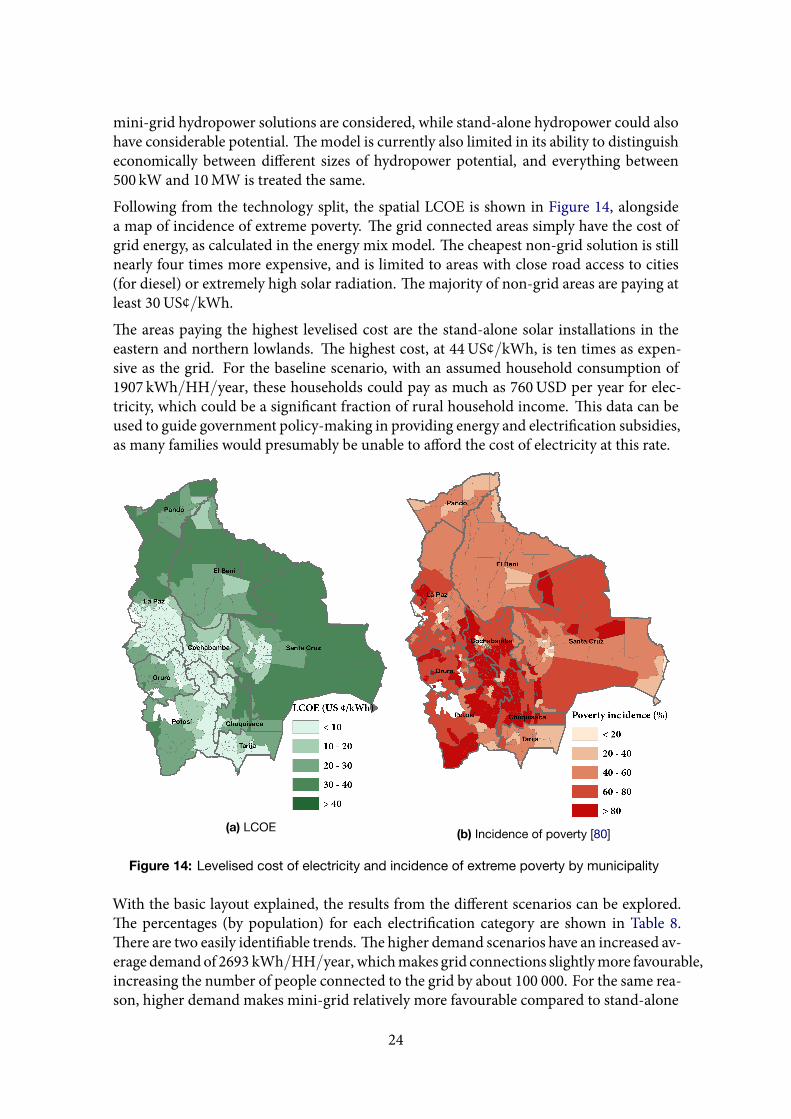
mini-grid hydropower solutions are considered, while stand-alone hydropower could alsohave considerable potential. The model is currently also limited in its ability to distinguisheconomically between different sizes of hydropower potential, and everything between500 kW and 10MW is treated the same.Following from the technology split, the spatial LCOE is shown in Figure 14, alongsidea map of incidence of extreme poverty. The grid connected areas simply have the cost ofgrid energy, as calculated in the energy mix model. The cheapest non-grid solution is stillnearly four times more expensive, and is limited to areas with close road access to cities(for diesel) or extremely high solar radiation. The majority of non-grid areas are paying atleast 30US¢/kWh.The areas paying the highest levelised cost are the stand-alone solar installations in theeastern and northern lowlands. The highest cost, at 44US¢/kWh, is ten times as expen-sive as the grid. For the baseline scenario, with an assumed household consumption of1907 kWh/HH/year, these households could pay as much as 760USD per year for elec-tricity, which could be a significant fraction of rural household income. This data can beused to guide government policy-making in providing energy and electrification subsidies,as many families would presumably be unable to afford the cost of electricity at this rate.

(a) LCOE (b) Incidence of poverty [80]

Figure 14: Levelised cost of electricity and incidence of extreme poverty by municipality

With the basic layout explained, the results from the different scenarios can be explored.The percentages (by population) for each electrification category are shown in Table 8.There are two easily identifiable trends. The higher demand scenarios have an increased av-erage demandof 2693 kWh/HH/year, whichmakes grid connections slightlymore favourable,increasing the number of people connected to the grid by about 100 000. For the same rea-son, higher demand makes mini-grid relatively more favourable compared to stand-alone

24

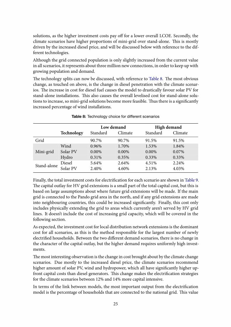
solutions, as the higher investment costs pay off for a lower overall LCOE. Secondly, theclimate scenarios have higher proportions of mini-grid over stand-alone. This is mostlydriven by the increased diesel price, and will be discussed below with reference to the dif-ferent technologies.Although the grid connected population is only slightly increased from the current valuein all scenarios, it represents about threemillion new connections, in order to keep upwithgrowing population and demand.The technology splits can now be discussed, with reference to Table 8. The most obviouschange, as touched on above, is the change in diesel penetration with the climate scenar-ios. The increase in cost for diesel fuel causes the model to drastically favour solar PV forstand-alone installations. This also causes the overall levelised cost for stand-alone solu-tions to increase, so mini-grid solutions become more feasible. Thus there is a significantlyincreased percentage of wind installations.

Table 8: Technology choice for different scenarios

Low demand High demandTechnology Standard Climate Standard Climate

Grid 90.7% 90.7% 91.5% 91.5%Wind 0.96% 1.70% 1.53% 1.84%Solar PV 0.00% 0.00% 0.00% 0.07%Mini-gridHydro 0.31% 0.35% 0.33% 0.33%

Stand-alone Diesel 5.64% 2.64% 4.51% 2.24%Solar PV 2.40% 4.60% 2.13% 4.03%

Finally, the total investment costs for electrification for each scenario are shown in Table 9.The capital outlay for HV grid extensions is a small part of the total capital cost, but this isbased on large assumptions about where future grid extensions will be made. If the maingrid is connected to the Pando grid area in the north, and if any grid extensions are madeinto neighbouring countries, this could be increased significantly. Finally, this cost onlyincludes physically extending the grid to areas which currently aren’t served by HV gridlines. It doesn’t include the cost of increasing grid capacity, which will be covered in thefollowing section.As expected, the investment cost for local distribution network extensions is the dominantcost for all scenarios, as this is the method responsible for the largest number of newlyelectrified households. Between the two different demand scenarios, there is no change inthe character of the capital outlay, but the higher demand requires uniformly high invest-ments.Themost interesting observation is the change in cost brought about by the climate changescenarios. Due mostly to the increased diesel price, the climate scenarios recommendhigher amount of solar PV, wind and hydropower, which all have significantly higher up-front capital costs than diesel generators. This change makes the electrification strategiesfor the climate scenarios between 12% and 14% more capital intensive.In terms of the link between models, the most important output from the electrificationmodel is the percentage of households that are connected to the national grid. This value

25

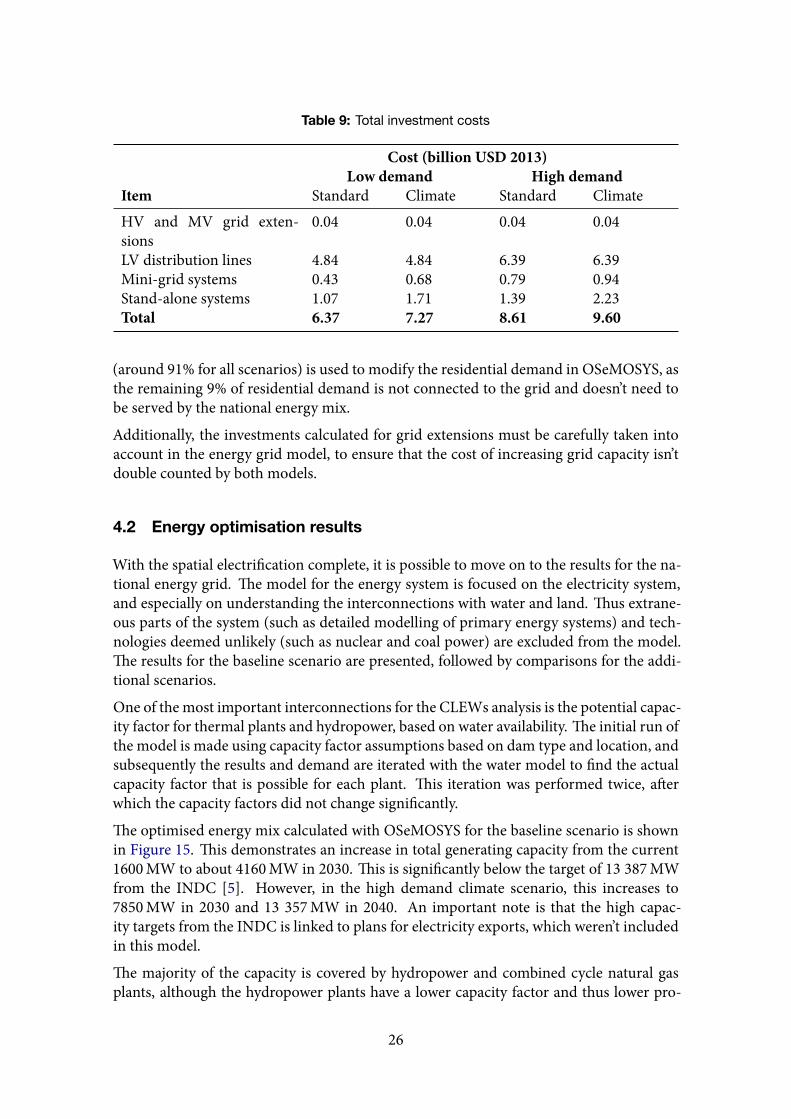
Table 9: Total investment costs

Cost (billion USD 2013)Low demand High demand

Item Standard Climate Standard ClimateHV and MV grid exten-sions

0.04 0.04 0.04 0.04

LV distribution lines 4.84 4.84 6.39 6.39Mini-grid systems 0.43 0.68 0.79 0.94Stand-alone systems 1.07 1.71 1.39 2.23Total 6.37 7.27 8.61 9.60

(around 91% for all scenarios) is used to modify the residential demand in OSeMOSYS, asthe remaining 9% of residential demand is not connected to the grid and doesn’t need tobe served by the national energy mix.

Additionally, the investments calculated for grid extensions must be carefully taken intoaccount in the energy grid model, to ensure that the cost of increasing grid capacity isn’tdouble counted by both models.

4.2 Energy optimisation results

With the spatial electrification complete, it is possible to move on to the results for the na-tional energy grid. The model for the energy system is focused on the electricity system,and especially on understanding the interconnections with water and land. Thus extrane-ous parts of the system (such as detailed modelling of primary energy systems) and tech-nologies deemed unlikely (such as nuclear and coal power) are excluded from the model.The results for the baseline scenario are presented, followed by comparisons for the addi-tional scenarios.

One of the most important interconnections for the CLEWs analysis is the potential capac-ity factor for thermal plants and hydropower, based on water availability. The initial run ofthe model is made using capacity factor assumptions based on dam type and location, andsubsequently the results and demand are iterated with the water model to find the actualcapacity factor that is possible for each plant. This iteration was performed twice, afterwhich the capacity factors did not change significantly.

The optimised energy mix calculated with OSeMOSYS for the baseline scenario is shownin Figure 15. This demonstrates an increase in total generating capacity from the current1600MW to about 4160MW in 2030. This is significantly below the target of 13 387MWfrom the INDC [5]. However, in the high demand climate scenario, this increases to7850MW in 2030 and 13 357MW in 2040. An important note is that the high capac-ity targets from the INDC is linked to plans for electricity exports, which weren’t includedin this model.

The majority of the capacity is covered by hydropower and combined cycle natural gasplants, although the hydropower plants have a lower capacity factor and thus lower pro-

26

2012 2016 2020 2024 2028 2032 2036 20400

1

2

3

4

5

Capaci

ty (GW

)

Natural gas (conventional)Natural gas (combined cycle)BiomassDieselGeothermalWindSolarHydro

Figure 15: Optimal energy capacity mix for baseline

duction. The conventional natural gas plants that make up most of the current fleet arecompletely phased out by 2032, being replaced by combined cycle plants.

There is a significant amount of diesel capacity installed in later years, but this is subject toa number of assumptions. This build-out of diesel power is mostly due to the fact that themodel is limited to planned natural gas plants until 2025, and after that there is a restrictionon the pace of installations. The diesel is thus a backstop technology, and shows the extracapacity required that won’t be met by existing plans. There is a small amount of solar,wind and biomass power in the results, but this is mostly accounted for by plants that arealready in the planning stage, and not necessarily chosen by the model’s algorithm.

The difference in actual output between natural gas and hydropower is made more clearin Figure 16, where hydropower is responsible on average for only about 30% of electricitygeneration. Thismakes it clear that natural gas will still be responsible for the vast majorityof Bolivia’s electricity production well into the future, under baseline assumptions.

2012 2016 2020 2024 2028 2032 2036 20400

20

40

60

80

100

Percentage share

NG (conventional)

NG (combined cycle)

Biomass

Diesel

Geothermal

Wind

Solar

Hydro0

2

4

6

8

LCOE (US c/kWh)

Figure 16: LCOE and production percentage by source

The LCOE curve (black line) shows the cumulative LCOE for each year. There is strongvariation at the beginning of the investment period as new investments are made, but thevalue steadies by about 2020. Past this period, the generation mix doesn’t change signifi-cantly, and since the costs were modelled without future increases, there is little reason forthe levelised cost to change.

27

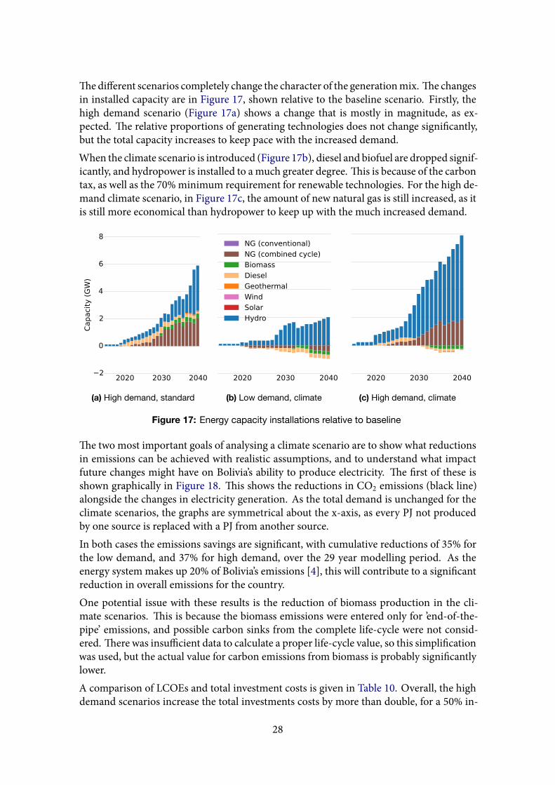
Thedifferent scenarios completely change the character of the generationmix. The changesin installed capacity are in Figure 17, shown relative to the baseline scenario. Firstly, thehigh demand scenario (Figure 17a) shows a change that is mostly in magnitude, as ex-pected. The relative proportions of generating technologies does not change significantly,but the total capacity increases to keep pace with the increased demand.When the climate scenario is introduced (Figure 17b), diesel and biofuel are dropped signif-icantly, and hydropower is installed to amuch greater degree. This is because of the carbontax, as well as the 70% minimum requirement for renewable technologies. For the high de-mand climate scenario, in Figure 17c, the amount of new natural gas is still increased, as itis still more economical than hydropower to keep up with the much increased demand.

2020 2030 2040−2

0

2

4

6

8

Capaci

ty (

GW

)

(a) High demand, standard

2020 2030 2040−2

0

2

4

6

8

NG (conventional)

NG (combined cycle)

Biomass

Diesel

Geothermal

Wind

Solar

Hydro

(b) Low demand, climate

2020 2030 2040−2

0

2

4

6

8

(c) High demand, climate

Figure 17: Energy capacity installations relative to baseline

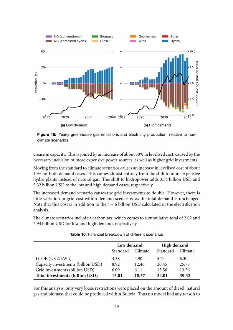
The two most important goals of analysing a climate scenario are to show what reductionsin emissions can be achieved with realistic assumptions, and to understand what impactfuture changes might have on Bolivia’s ability to produce electricity. The first of these isshown graphically in Figure 18. This shows the reductions in CO2 emissions (black line)alongside the changes in electricity generation. As the total demand is unchanged for theclimate scenarios, the graphs are symmetrical about the x-axis, as every PJ not producedby one source is replaced with a PJ from another source.In both cases the emissions savings are significant, with cumulative reductions of 35% forthe low demand, and 37% for high demand, over the 29 year modelling period. As theenergy system makes up 20% of Bolivia’s emissions [4], this will contribute to a significantreduction in overall emissions for the country.One potential issue with these results is the reduction of biomass production in the cli-mate scenarios. This is because the biomass emissions were entered only for ’end-of-the-pipe’ emissions, and possible carbon sinks from the complete life-cycle were not consid-ered. There was insufficient data to calculate a proper life-cycle value, so this simplificationwas used, but the actual value for carbon emissions from biomass is probably significantlylower.A comparison of LCOEs and total investment costs is given in Table 10. Overall, the highdemand scenarios increase the total investments costs by more than double, for a 50% in-

28

2012 2020 2030 2040

−30

0

30

60

Pro

duct

ion (

PJ)

NG (conventional)

NG (combined cycle)

Biomass

Diesel

Carbon savings (million tons)

(a) Low demand

2012 2020 2030 2040

−30

0

30

60

Geothermal

Wind

Solar

Hydro

0.0

2.5

5.0

7.5

10.0

Carb

on s

avin

gs

(mill

ion t

ons)

(b) High demand

Figure 18: Yearly greenhouse gas emissions and electricity production, relative to non-climate scenarios

crease in capacity. This is joined by an increase of about 30% in levelised cost, caused by thenecessary inclusion of more expensive power sources, as well as higher grid investments.

Moving from the standard to climate scenarios causes an increase in levelised cost of about10% for both demand cases. This comes almost entirely from the shift to more expensivehydro plants instead of natural gas. This shift to hydropower adds 3.54 billion USD and5.32 billion USD to the low and high demand cases, respectively.

The increased demand scenario causes the grid investments to double. However, there islittle variation in grid cost within demand scenarios, as the total demand is unchanged.Note that this cost is in addition to the 4 – 6 billion USD calculated in the electrificationanalysis.

The climate scenarios include a carbon tax, which comes to a cumulative total of 2.02 and2.94 billion USD for low and high demand, respectively.

Table 10: Financial breakdown of different scenarios

Low demand High demandStandard Climate Standard Climate

LCOE (US ¢/kWh) 4.38 4.90 5.74 6.30Capacity investments (billion USD) 8.92 12.46 20.45 25.77Grid investments (billion USD) 6.09 6.11 13.56 13.56Total investments (billion USD) 15.01 18.57 34.01 39.32

For this analysis, only very loose restrictions were placed on the amount of diesel, naturalgas and biomass that could be produced within Bolivia. Thus no model had any reason to

29

resort to more expensive imports. This is an oversimplification, as although local oil pro-duction is sufficient for domestic needs, about 30% of refined oil products are imported[23], as local refining capacity is limited. This doesn’t apply to natural gas, which needsminimal processing. Under the high demand scenario, the energy system will be consum-ing about 5.5 billion m3 of natural gas per year by 2040, which represents just over 11% ofcurrent production [81]. Currently, electricity plants consume about 7% of the gas produc-tion [23]. Future natural gas reserves will be the biggest deciding factor, but it is possiblethat larger increases in domestic use could have a significant impact on Bolivia’s ability toearn from natural gas exports.

4.3 Water modelling results

With the water model fully set up and calibrated, the yearly energy demands for each sce-nario are entered from the energy models. This creates a demand for each plant that themodel will try tomeet, and shortfalls can be inserted back into the energymodel as reducedcapacity factors.

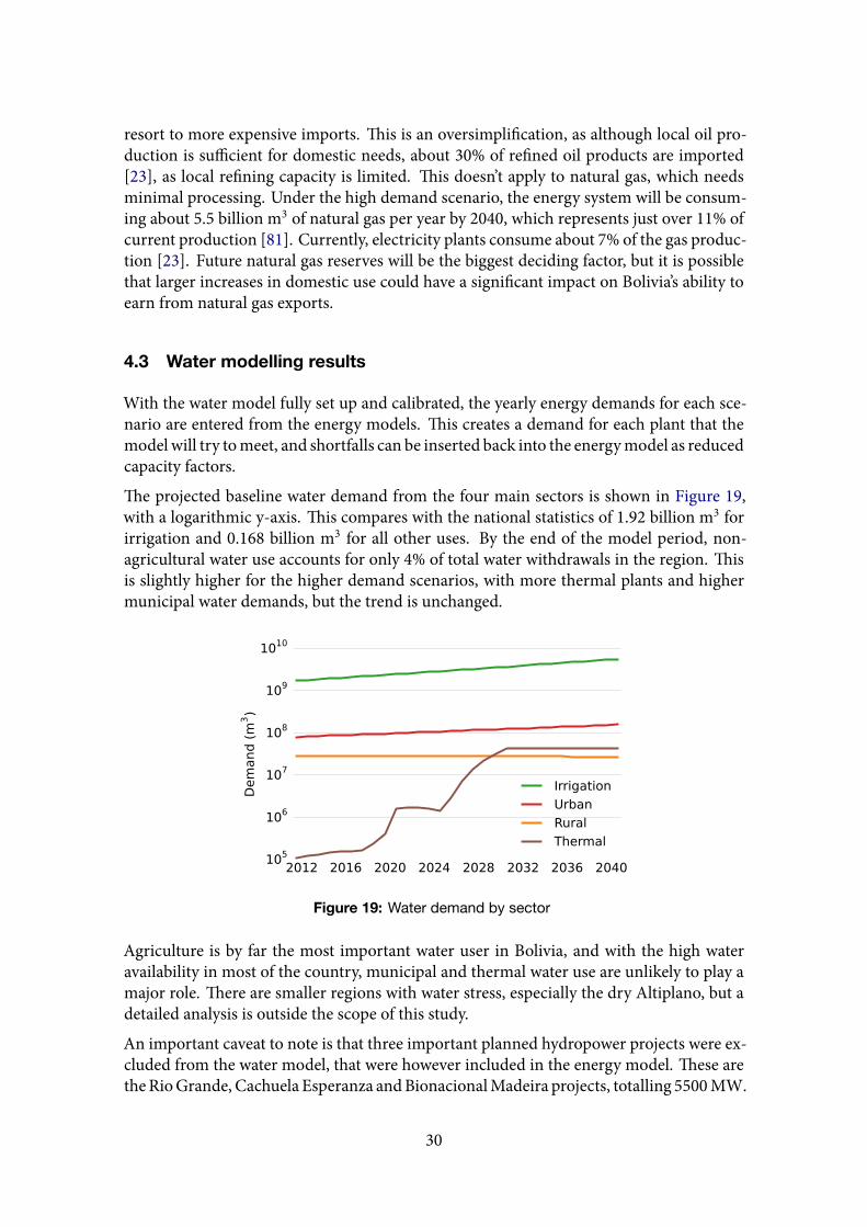
The projected baseline water demand from the four main sectors is shown in Figure 19,with a logarithmic y-axis. This compares with the national statistics of 1.92 billion m3 forirrigation and 0.168 billion m3 for all other uses. By the end of the model period, non-agricultural water use accounts for only 4% of total water withdrawals in the region. Thisis slightly higher for the higher demand scenarios, with more thermal plants and highermunicipal water demands, but the trend is unchanged.

2012 2016 2020 2024 2028 2032 2036 2040105

106

107

108

109

1010

Demand (m

3)

Irrigation

Urban

Rural

Thermal

Figure 19: Water demand by sector

Agriculture is by far the most important water user in Bolivia, and with the high wateravailability in most of the country, municipal and thermal water use are unlikely to play amajor role. There are smaller regions with water stress, especially the dry Altiplano, but adetailed analysis is outside the scope of this study.

An important caveat to note is that three important planned hydropower projects were ex-cluded from the water model, that were however included in the energy model. These aretheRioGrande, Cachuela Esperanza andBionacionalMadeira projects, totalling 5500MW.

30

Thefirst was excluded due to a lack of data on location and characteristics, while the secondtwo fell outside the analysed region. These three projects provide a considerable percent-age of electricity generation in all but the baseline scenario (from 5% to 30%). For thisanalysis, they are given the same capacity factors as the Rositas project, which is the mostsimilar in terms of size, type and location.

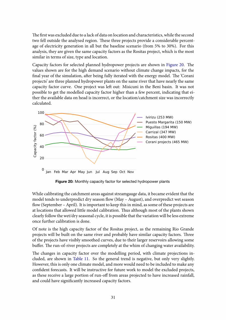
Capacity factors for selected planned hydropower projects are shown in Figure 20. Thevalues shown are for the high demand scenario without climate change impacts, for thefinal year of the simulation, after being fully iterated with the energy model. The ’Coraniprojects’ are three planned hydropower plants on the same river that have nearly the samecapacity factor curve. One project was left out: Misicuni in the Beni basin. It was notpossible to get the modelled capacity factor higher than a few percent, indicating that ei-ther the available data on head is incorrect, or the location/catchment size was incorrectlycalculated.

Jan Feb Mar Apr May Jun Jul Aug Sep Oct Nov0

20

40

60

80

100

Ca

pa

city

fa

cto

r (%

)

Ivirizu (253 MW)

Puesto Margarita (150 MW)

Miguillas (194 MW)

Carrizal (347 MW)

Rositas (400 MW)

Corani projects (465 MW)

Figure 20: Monthly capacity factor for selected hydropower plants

While calibrating the catchment areas against streamgauge data, it became evident that themodel tends to underpredict dry season flow (May – August), and overpredict wet seasonflow (September – April). It is important to keep this inmind, as some of these projects areat locations that allowed little model calibration. Thus although most of the plants shownclearly follow the wet/dry seasonal cycle, it is possible that the variation will be less extremeonce further calibration is done.

Of note is the high capacity factor of the Rositas project, as the remaining Rio Grandeprojects will be built on the same river and probably have similar capacity factors. Threeof the projects have visibly smoothed curves, due to their larger reservoirs allowing somebuffer. The run-of-river projects are completely at the whim of changing water availability.

The changes in capacity factor over the modelling period, with climate projections in-cluded, are shown in Table 11. So the general trend is negative, but only very slightly.However, this is only one climate model, and more would need to be included to make anyconfident forecasts. It will be instructive for future work to model the excluded projects,as these receive a large portion of run-off from areas projected to have increased rainfall,and could have significantly increased capacity factors.

31

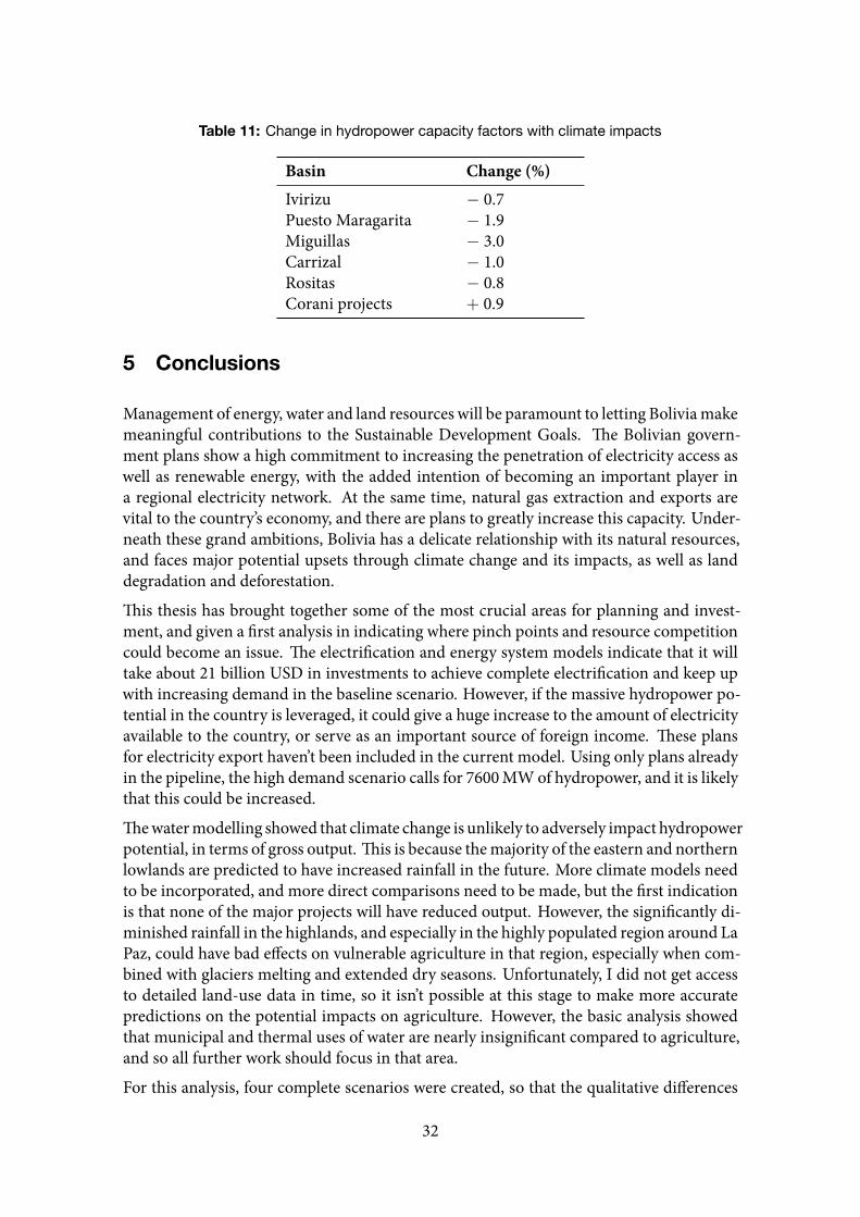
Table 11: Change in hydropower capacity factors with climate impacts

Basin Change (%)Ivirizu − 0.7Puesto Maragarita − 1.9Miguillas − 3.0Carrizal − 1.0Rositas − 0.8Corani projects + 0.9

5 Conclusions

Management of energy, water and land resources will be paramount to letting Boliviamakemeaningful contributions to the Sustainable Development Goals. The Bolivian govern-ment plans show a high commitment to increasing the penetration of electricity access aswell as renewable energy, with the added intention of becoming an important player ina regional electricity network. At the same time, natural gas extraction and exports arevital to the country’s economy, and there are plans to greatly increase this capacity. Under-neath these grand ambitions, Bolivia has a delicate relationship with its natural resources,and faces major potential upsets through climate change and its impacts, as well as landdegradation and deforestation.

This thesis has brought together some of the most crucial areas for planning and invest-ment, and given a first analysis in indicating where pinch points and resource competitioncould become an issue. The electrification and energy system models indicate that it willtake about 21 billion USD in investments to achieve complete electrification and keep upwith increasing demand in the baseline scenario. However, if the massive hydropower po-tential in the country is leveraged, it could give a huge increase to the amount of electricityavailable to the country, or serve as an important source of foreign income. These plansfor electricity export haven’t been included in the current model. Using only plans alreadyin the pipeline, the high demand scenario calls for 7600MW of hydropower, and it is likelythat this could be increased.

Thewatermodelling showed that climate change is unlikely to adversely impact hydropowerpotential, in terms of gross output. This is because themajority of the eastern and northernlowlands are predicted to have increased rainfall in the future. More climate models needto be incorporated, and more direct comparisons need to be made, but the first indicationis that none of the major projects will have reduced output. However, the significantly di-minished rainfall in the highlands, and especially in the highly populated region around LaPaz, could have bad effects on vulnerable agriculture in that region, especially when com-bined with glaciers melting and extended dry seasons. Unfortunately, I did not get accessto detailed land-use data in time, so it isn’t possible at this stage to make more accuratepredictions on the potential impacts on agriculture. However, the basic analysis showedthat municipal and thermal uses of water are nearly insignificant compared to agriculture,and so all further work should focus in that area.

For this analysis, four complete scenarios were created, so that the qualitative differences

32

between them could be compared. However, in order to quantify the potential impactsof different assumptions and scenarios, it will be useful to perform the analysis with somevariables controlled. This will allow the direct impacts of climate change, with and withouta government response, to be measured. In addition, many more climate models and sce-narios should be included, as this project included only one. This will show a much widerrange of possible positive and negative impacts, and allow the problem to be more fullyunderstood. Nevertheless, the results show that even with a high demand scenario, andclimate change included, Bolivia can achieve most of its INDC goals, decrease its depen-dence on carbon, and have more electricity and natural gas available to export.

6 Discussion

Apart from the analysis of Bolivia, this thesis has served as a case study of an extendedCLEWsmethodology. The energy-water nexus is a topic gaining increasing attention as theimportance of these interactions are realised. Here the nexus is extended to include climatechange, land-use, as well as electricity access, with all potential connections mapped out.

The results indicate that this extended framework is indeed worth the effort. All of thedifferent categories have important links with each other, and by modelling them togetherit is possible to understand the extent to which these links alter the results. However, someof the links are relatively minor, and it is easy to predict their influence without completemodelling (such as the percentage grid connected, fed from ONSSET into OSeMOSYS).The most important connections are the levelised cost of electricity, the hydropower de-mand projections, the hydropower capacity factors, the water available to agriculture, andof course, the impacts of climate change on all of these.

Nonetheless, there are significant limitations in this project, imposed by intrinsic modellimitations, data access as well as time. The primary limitation of the electricity accessmodel is that is has no temporal aspect, and assumed overnight investments for an out-come state in 2030. Additionally, the lack of some data (most importantly detailed currentelectricity access data) meant that significant assumptions has to be made. The energy op-timisation model made large simplifying assumptions, and didn’t consider limitations inregional interconnects, nor did it model primary energy sources in any detail. Most im-portantly, the water model did not cover the entire country, and excluded two very largehydropower projects, as well as huge areas of agricultural and pasture land. Finally, theland-use and aquifers were modelled very simply, which means that the calculated runoffcan’t have complete confidence.

33

References

[1] International Energy Agency. World Energy Outlook 2015. 2015. isbn: 978-92-64-24365-1. url: https://www.iea.org/bookshop/700-World_Energy_Outlook_2015.

[2] FAO. FAO Country Profile: Bolivia. Tech. rep. 2016, pp. 1–9. url: http://faostat3.fao.org/home/E.

[3] FAO.Aquastat: Bolivia. Tech. rep. 2016. url: http://www.fao.org/nr/water/aquastat/data/query/results.html.

[4] UNFCCC. UNFCCC Country Brief 2014: Bolivia (Plurinational State of). Tech. rep.2014. url: http://newsroom.unfccc.int/media/437221/country-brief-bolivia.pdf.

[5] Intended Nationally Determined Contribution from the Plurinational State of Bolivia.Tech. rep. 2015. url: http : / /www4.unfccc . int / submissions / INDC/Published%20Documents/Bolivia/1/INDC-Bolivia-english.pdf.

[6] J. M.Thibeault, A. Seth, andM. Garcia. “Changing climate in the Bolivian Altiplano:CMIP3 projections for temperature and precipitation extremes”. In: Journal of Geo-physical Research Atmospheres 115.8 (2010), pp. 1–18. doi: 10.1029/2009JD012718.

[7] MVuille, R S Bradley,MWerner, and Frank Keimig. “20th Century Climate Changein the Tropical Andes Observations and Model Results”. In: Climatic Change 59(2003), pp. 75–99.

[8] B.C. Bates, Z.W. Kundzewicz, S. Wu, and J.P. Palutikof. Climate Change and Water.2008, p. 210. doi: 10.1016/j.jmb.2010.08.039.

[9] United Nations. Sustainable Development Goals. 2015. url: http : / /www.un.org/sustainabledevelopment/sustainable-development-goals/ (visited on 04/02/2016).

[10] DimitriosMentis,ManuelWelsch, Francesco FusoNerini, Oliver Broad,MarkHow-ells, Morgan Bazilian, and Holger Rogner. “A GIS-based approach for electrificationplanning — A case study on Nigeria”. In: Energy for Sustainable Development 29(2015), pp. 142–150. doi: 10.1016/j.esd.2015.09.007.

[11] Mark Howells, Holger Rogner, Neil Strachan, Charles Heaps, Hillard Huntington,Socrates Kypreos, Alison Hughes, Semida Silveira, Joe DeCarolis, Morgan Bazillian,and Alexander Roehrl. “OSeMOSYS: The Open Source Energy Modeling System.An introduction to its ethos, structure and development.” In: Energy Policy 39.10(2011), pp. 5850–5870. doi: 10.1016/j.enpol.2011.06.033.

[12] Jack Sieber and David Purkey. Water Evaluation And Planning System. Tech. rep.Somerville, MA: Stockholm Environmental Institute, 2013. url: http://www.sei-international . org /mediamanager / documents / Programmes /Water - sanitation /WEAP-brochure-A4-May2013.pdf.

[13] Günther Fischer, Freddy O. Nachtergaele, Sylvia Prieler, Edmar Teixeira, Géza Tóth,Harrij Van Velthuizen, Luc Verelst, and DavidWiberg.Global Agro-Ecological Zones(GAEZ v3.0). Tech. rep. Laxenburg, Austria: IIASA/FAO, 2012. url: http://www.gaez.iiasa.ac.at/docs/GAEZ_User_Guide.pdf.

34

[14] Department of Economic and Social Affairs of the United Nations. World StatisticsPocketbook 2015 edition. New York: United Natuons, 2015. isbn: 978-9211-6157-08.url: http://data.un.org/CountryProfile.aspx?crName=Bolivia%20(Plurinational%20State%20of).

[15] The World Bank.World Development Indicators. 2016. url: http://databank.worldbank.org/data/reports.aspx?source=2&country=BOL&series=&period= (visited on03/03/2016).

[16] Euromonitor. Economic Trends and Consumer Lifestyles. 2013. url: http : / /www .euromonitor .com/bolivia- in- 2030- the- future- demographic/report (visited on03/03/2016).

[17] G. Magrin, C. Gay Garcia, D. Cruz Choque, J.C. Gimenez, A.R. Moreno, G.J. Nagy,C. Nobre, and A Villamizar. “Climate Change 2007: Impacts, Adaptation and Vul-nerability Contribution of Working Group II to the Fourth Assessment Report ofthe Intergovernmental Panel on Climate Change”. In: Genebra, Suíça. Cambridge,U.K.: Cambridge University Press, 2007. Chap. Latin Amer, pp. 581–615. isbn: 978-052-1880-107. url: https://www.ipcc.ch/pdf/assessment- report/ar4/wg2/ar4_wg2_full_report.pdf.

[18] Peter G. Jones and Philip K. Thornton. “The potential impacts of climate change onmaize production in Africa and Latin America in 2055”. In: Global EnvironmentalChange 13.1 (2003), pp. 51–59. doi: 10.1016/S0959-3780(02)00090-0.

[19] CDIAC.CarbonDioxide Emissions (CO2),ThousandMetric Tons of CO2MillenniumDevelopment Goals Indicators. 2015. url: http://mdgs.un.org/unsd/mdg/data.aspx(visited on 03/07/2015).

[20] Julia Z. McDowell and Jeremy J. Hess. “Accessing adaptation: Multiple stressors onlivelihoods in the Bolivian highlands under a changing climate”. In: Global Environ-mental Change 22.2 (2012), pp. 342–352. doi: 10.1016/j.gloenvcha.2011.11.002.

[21] Ministerio de Desarrollo Rural y Tierras. Plan del Sector: Sector Desarrollo Agro-pecuario 2014 - 2018 ”Hacia el 2025”. Tech. rep. La Paz, 2014.

[22] Comité Nacional de Despacho de Carga. Sector Eléctrico en Bolivia. 2016. url: http://www.cndc.bo/sin/index.php (visited on 01/27/2016).

[23] International Energy Agency. Bolivia: Balances for 2013. Tech. rep. 2013. url: https:/ /www . iea . org / statistics / statisticssearch / report / ?country=Bolivia&product=balances.

[24] USGS.Mineral operations outside theUnited States: Bolivia. 2015. url: http://mrdata.usgs.gov/mineral-operations/output/minfac-fBL.html (visited on 03/07/2016).

[25] L.E. Andersen andM.Meza. “TheNaturalGas Sector in Bolivia: AnOverview”. 2001.url: http://www.iisec.ucb.edu.bo/papers/2001-2005/iisec-dt-2001-01.pdf.

[26] EIA. Bolivia Overview. 2015. url: https://www.eia.gov/beta/international/analysis.cfm?iso=BOL (visited on 03/07/2016).

[27] USDepartment of Energy.An Energy Overview of Bolivia. Tech. rep. 2013. url: http://www.osti.gov/scitech/servlets/purl/821117.

35

[28] Comité Nacional de Despacho de Carga. Instalaciones de Generación. 2014. url: http://www.cndc.bo/agentes/generacion.php (visited on 03/07/2016).

[29] ComitéNacional deDespacho deCarga. Instalaciones de Transmisión en el STI. 2014.url: http://www.cndc.bo/agentes/transmision.php (visited on 03/07/2016).

[30] Comité Nacional de Despacho de Carga. Empresas de Distribución. 2014. url: http://www.cndc.bo/agentes/distribucion.php (visited on 03/07/2016).

[31] Dan Keane.Morales’ Gas Nationalization Complete. 2006. url: http://www.washingtonpost.com/wp-dyn/content/article/2006/10/29/AR2006102900036.html (visitedon 03/07/2016).

[32] FAO. Country report: Bolivia (Estado Plurinacional de). Tech. rep. 2015. url: http://www.fao.org/nr/water/aquastat/countries_regions/BOL/index.stm.

[33] Peter H. Gleick. The World’s Water. Volume 7. The Biennial Report on FreshwaterResources. Washington, DC: Island Press, 2012. isbn: 978-1-59726-998-8. url: http://link.springer.com/book/10.1007/978-1-59726-228-6.

[34] S. Szabó, K. Bódis, T. Huld, and M. Moner-Girona. “Sustainable energy planning:Leapfrogging the energy poverty gap in Africa”. In: Renewable and Sustainable En-ergy Reviews 28 (2013), pp. 500–509. doi: 10.1016/j.rser.2013.08.044.

[35] Roberto Peredo Echazú, Hortensia Jiménez Rivera, and Juan Manuel Gonzáles Flo-res. Plan de Universalizacion Bolivia con Energía 2010 - 2025. Tech. rep. La Paz: Min-isterio de Hidrocarburos y Energia, 2010. url: http://www2.hidrocarburos.gob.bo/phocadownload/PLAN%20DE%20UNIVERSALIZACI%C3%93N%20BOLIVIA%20CON%20ENERG%C3%8DA.pdf.

[36] DimitrisMentis,MarkHowells,HolgerRogner, EduardoZepeda, Shahid Siyal,OliverBroad, Morgan Bazilian, and Ad Roo. “Lighting up the World”. In: (), pp. 1–15.

[37] Python Software Foundation. Python. 2016. url: https://www.python.org/ (visitedon 04/02/2016).

[38] Robert Hijmans. Global Administrative Areas. 2009. url: http://gadm.org/version2(visited on 03/08/2016).

[39] WorldPop. Bolivia Population Map. 2014. url: http://www.worldpop.org.uk/data/(visited on 03/08/2016).

[40] Paul W. Stackhouse. NASA Surface meteorology and Solar Energy: Global Data Sets.2016. url: https://eosweb.larc.nasa.gov/cgi-bin/sse/global.cgi?email=skip@larc.nasa.gov (visited on 03/08/2016).

[41] Steve Kempler. Goddard Earth Sciences Data and Information Services Center. 2011.url: http://disc.sci.gsfc.nasa.gov/mdisc/data-holdings (visited on 03/08/2016).

[42] A. Jarvis, H.I. Reuter, A. Nelson, and E. Guevara.Hole-filled seamless SRTM data V4.2008. url: http://www.cgiar-csi.org/data/srtm-90m-digital-elevation-database-v4-1#download (visited on 03/08/2016).

[43] ProtectedPlanet.Bolivia (Plurinational State of), Latin America andCaribbean. 2015.url: http://www.protectedplanet.net/country/BO (visited on 03/08/2016).

36

[44] GIS-LAB. VMap0 data in ESRI shape format. 2014. url: http : / /gis - lab . info/qa/vmap0-eng.html (visited on 03/08/2016).

[45] A. Nelson. Estimated travel time to the nearest city of 50,000 or more people in year2000. 2008. url: http : / / forobs . jrc .ec .europa .eu/products /gam/download .php(visited on 03/08/2016).

[46] Joint Research Centre of the European Commission. Mean annual streamflow perunit area (estimated). 2016. url: http://water.jrc.ec.europa.eu/waterportal/ (visitedon 03/08/2016).

[47] USGS. HydroSHEDS. 2008. url: http://hydrosheds.cr.usgs.gov/index.php (visitedon 03/08/2016).

[48] A Schneider, M Friedl, and D Potere. “A new map of global urban extent fromMODIS data”. In: Environmental Research Letters 4 (2009). url: https : / / nelson .wisc.edu/sage/data-and-models/schneider.php.

[49] NASA. Earth at Night. 2012. url: http : / / earthobservatory . nasa . gov / Features /NightLights/page3.php (visited on 04/02/2016).

[50] World Bank. Pump price for diesel fuel (USD per liter). 2014. url: http://data.worldbank.org/indicator/EP.PMP.DESL.CD (visited on 02/27/2016).

[51] Bob Boundy, Susan W. Diegel, Lynn Wright, and Stacy C. Davis. Biomass EnergyData Book. Oak Ridge National Laboratory, 2011, p. 2011.

[52] World Bank. Energy Sector Management Assistance Program. 2016. url: https : / /esmap.org/dlmv698-3545 (visited on 03/02/2016).

[53] IRENA. “Hydropower”. In:Renewable EnergyTechnologies: CostAnalysis Series (2012).[54] IRENA. “WindPower”. In:Renewable EnergyTechnologies: CostAnalysis Series (2012).[55] IRENA. “Solar Photovoltaics”. In: Renewable Energy Technologies: Cost Analysis Se-

ries (2012).[56] Francesco Fuso Nerini, Oliver Broad, Dimitris Mentis, Manuel Welsch, Morgan

Bazilian, and Mark Howells. “A cost comparison of technology approaches for im-proving access to electricity services”. In: Energy2 95 (2016), pp. 255–265. doi: 10.1016/j.energy.2015.11.068.

[57] Sustainable Energy for All.Global Tracking Framework. Tech. rep.World Bank, 2013,p. 101.

[58] FAO.Components of the IncomeAggregate: ”Encuesta deHogares, Bolivia 2005”. Tech.rep. 2010. url: http : / /www. fao .org / fileadmin/ templates / riga /docs /Country_survey_information/35_Bolivia05-Components_of_the_Income_Aggregate.pdf.

[59] Gabriella Balderrama. “UnfinishedPhD thesis onBolivia”. PhD.KTHRoyal Instituteof Technology, 2016.

[60] Microsoft. Offiial VBA language reference. 2016. url: https://msdn.microsoft.com/en-us/library/office/gg264383.aspx (visited on 04/02/2016).

[61] Comité Nacional de Despacho de Carga. Estadistica Anual. 2016. url: http://www.cndc.bo/estadisticas/anual.php (visited on 01/20/2016).

37

[62] Comité Nacional de Despacho de Carga. Solicitudas de información (Informationrequests). La Paz, Bolivia, 2016.

[63] PLATTS. World Electric Power Plants Database. Tech. rep. McGraw Hilll Financial,2015. url: http://www.platts.com/products/world-electric-power-plants-database.

[64] Rajan Gupta and Harihar Shankar. Global Energy Observatory. 2016. url: http : / /globalenergyobservatory.org/ (visited on 03/02/2016).

[65] Darío R. Gómez and John D. Watterson. 2006 IPCC Guidelines for National Green-house Gas Inventories. Tech. rep. 2006.

[66] IPCC. Direct Global Warming Potentials. 2007. url: https://www.ipcc.ch/publications_and_data/ar4/wg1/en/ch2s2-10-2.html (visited on 05/10/2016).

[67] Silvia Ulloa Jimenez. “Nicaragua WEAP model: Supporting a CLEWS nexus assess-ment”. 2016.

[68] Senamhi. Servicio Nacional de Meteorología e Hidrología. 2016.[69] C.J. Vörösmarty, B. Fekete, and B.A. Tucker. River Discharge Database, Version 1.0

(RivDIS v1.0), Volumes 0 through 6. A contribution to IHP-VTheme 1. Technical Doc-uments in Hydrology Series. Tech. rep. Paris: UNESCO, 1996.

[70] FAO. FAOClim-NET. 1990. url: http://geonetwork3.fao.org/climpag/agroclimdb_en.php (visited on 05/12/2016).

[71] USGS. Land Cover Type Yearly L3 Global 0.05Deg CMG. 2012. url: https://lpdaac.usgs.gov/dataset_discovery/modis/modis_products_table/mcd12c1 (visited on04/05/2016).

[72] Empresa Electrica Corani S.A. Proyectos Hidroelectricos. 2016. url: http : / /www .corani.com/index.php/styles/hidroelectricos/ambrosia (visited on 04/10/2016).

[73] BN Americas. Electric Power - Bolivia. url: http://www.bnamericas.com/project-profile/en/banda-azul-hydro-central-banda-azul (visited on 04/10/2016).

[74] Empresa Electrica Valle Hermoso S.A. Cetrales Electricas. 2016. url: http://www.evh.bo/index.php/ce/pc (visited on 04/10/2016).

[75] Göran Berndes. “Bioenergy and water - The implications of large-scale bioenergyproduction for water use and supply”. In: Global Environmental Change 12.4 (2002),pp. 253–271. doi: 10.1016/S0959-3780(02)00040-7.

[76] National Energy Technology Laboratory. Estimating Freshwater Needs to Meet Fu-ture Thermoelectric Generation Requirements: 2009 Update. Tech. rep. DOE/NETL-400/2010/1339. 2009. url: http://www.netl.doe.gov/energy-analyses/pubs/2010_Water_Needs_Analysis.pdf.

[77] Vasilis Fthenakis and Hyung Chul Kim. “Life-cycle uses of water in U.S. electricitygeneration”. In: Renewable and Sustainable Energy Reviews 14.7 (2010), pp. 2039–2048. doi: 10.1016/j.rser.2010.03.008.

[78] Anthony C. Hirst, Hal B. Gordon, and Siobhan P. O’Farrell. “Global warming in acoupled climate model including oceanic eddy-induced advection”. In: GeophysicalResearch Letters 23.23 (1996), p. 3361. issn: 0094-8276. doi: 10.1029/96GL03234.

38

[79] IPCC. B2 Storyline and Scenario Family. 2016. url: http://www.ipcc.ch/ipccreports/sres/emission/index.php?idp=95.

[80] Unidad de Análisis de Políticas Sociales y Económicas. Mapa de incidencia de po-breza extrema. 2001. url: http://geo.gob.bo/geonetwork/apps/georchestra/?uuid=af587c2c-65cd-4adf-bfa0-ab9e3a46fb0e (visited on 05/10/2016).

[81] CIA.Natural gas - production compares the total natural gas produced in cubic meters(cu m). 2016. url: https://www.cia.gov/library/publications/the-world-factbook/rankorder/2249rank.html (visited on 05/10/2016).

39

Appendix A Python code: ONSSET data extraction

def createSet t lements ( set t lements , pop , popPer , s i ze ) :# c l i p and pro j ec t

# resample to the chosen s i zeResample_management ( pop , ' temp ' , s ize , 'BILINEAR ' )# and create the new po in t l a ye rRasterToPoint_convers ion ( ' temp ' , set t lements )# add x and y po in tsAddXY_management ( set t lements )

# add the new values f o r the points , using the r a t i o of the new ce l l s to the↪→ o r i g i n a l

AddField_management ( set t lements , ' Populat ion ' , 'LONG' )CalculateField_management ( set t lements , ' Populat ion ' , ' ! gr id_code ! ␣*␣ ' + st r (

↪→ s i ze * s i ze / popPer ) , 'PYTHON_9.3 ' )

# rename and clean up# done t h i s way ( as opposed to A l t e r F i e l d ) so tha t the f i e l d type can be

↪→ spec i f i edAddField_management ( set t lements , 'X ' , 'LONG' )CalculateField_management ( set t lements , 'X ' , ' ! POINT_X ! ' , 'PYTHON_9.3 ' )DeleteField_management ( set t lements , 'POINT_X ' )AddField_management ( set t lements , 'Y ' , 'LONG' )CalculateField_management ( set t lements , 'Y ' , ' ! POINT_Y ! ' , 'PYTHON_9.3 ' )DeleteField_management ( set t lements , 'POINT_Y ' )DeleteField_management ( set t lements , ' po i n t i d ; ␣grid_code ' )

# end createSet t lements

def isUrban ( set t lements , ta rge tPercent ) :ca lcu la ted = 1.0 # va r i ab l e used to s tore ca lcu la ted urban f r a c t i o nta rge t = ta rgetPercent /100 # ta rge t f r a c t i o nurbanCutoff = 1000.0 # s t a r t i n g guess f o r urban cu to f f dens i tycont = TrueAddField_management ( set t lements , ' temp_urban ' , 'LONG' )

while cont :

# sum the t o t a l populat iont o t a l = 0.0with da . SearchCursor ( set t lements , ' Populat ion ' ) as cursor :

for row in cursor :t o t a l += row [ 0 ]

# use the cur ren t cu to f f and i n s e r t populat ions f o r every urban set t lementcodeblock = """ def getClass ( populat ion ) :

i f populat ion > """ + st r ( urbanCutoff ) + " " " :r e tu rn populat ion

e lse :r e tu rn 0 """

CalculateField_management ( set t lements , ' temp_urban ' , ' getClass ( ! Populat ion↪→ ! ) ' , 'PYTHON_9.3 ' , codeblock )

# sum the urban populat ion

40

urbanTota l = 0.0with da . SearchCursor ( set t lements , " temp_urban" ) as cursor :

for row in cursor :urbanTota l += row [ 0 ]

ca lcu la ted = urbanTota l / t o t a l

i f abs ( t a rge t - ca lcu la ted ) < 0.001:# i f the ca lcu la ted i s w i t h i n 0.5 percentage po in ts then i t ' s good

↪→ enoughcont = False # so we qu i te the loop

else :# otherwise nudge the cu to f f a b i t i n the r i g h t d i r e c t i o ni f ca lcu la ted > ta rge t :

urbanCutoff += urbanCutoff * 2 * abs ( 1 - ca lcu la ted / t a rge t )else :

urbanCutoff -= urbanCutoff * 2 * abs ( 1 - ca lcu la ted / t a rge t )# end whi le

# create the new f i e l d and spec i f i y the cu to f f va lue usedAddField_management ( set t lements , ' IsUrban_ ' + st r ( i n t ( urbanCutof f ) ) , 'SHORT ' )codeblock = """ def getClass ( populat ion ) :

i f populat ion > """ + st r ( urbanCutoff ) + " " " :r e tu rn 1

e lse :r e tu rn 0 """

CalculateField_management ( set t lements , ' IsUrban_ ' + st r ( i n t ( urbanCutoff ) ) , '↪→ getClass ( ! Populat ion ! ) ' , 'PYTHON_9.3 ' , codeblock )

# clean upDeleteField_management ( set t lements , ' temp_urban ' )

# end isUrban

def getPV ( set t lements , ghi , s i ze ) :# import from csv# c l i p and pro j ec t

# create a r a s t e r f o r the so l a r data using the spec i f i ed c e l l s i zesp l i ne = sa . Sp l ine ( ghi , 'Ann ' , s i ze )sp l i ne . save ( ' temp ' )# and i n s e r t i n t o set t lementssa . Ext rac tMu l t iVa luesToPo in ts ( set t lements , [ [ ' temp ' , ' ghi_day ' ] ] )

# ca l cu l a t e the yea r l y va lue by mu l t i p l y i ng by 365AddField_management ( set t lements , ' GHI_annual ' , 'LONG' )CalculateField_management ( set t lements , ' GHI_annual ' , ' ! ghi_day ! ␣*␣365 ' , '

↪→ PYTHON_9.3 ' )

# clean upDeleteField_management ( set t lements , ' ghi_day ' )

# ca l cu l a t e the PV cost based on GHI , by i n t e r po l a t i n g from the fo l l ow ing two↪→ poin ts from Szabo2013

# 1800 kWh/m2/ year - 0.24 USD/kWh# 2600 kWh/m2/ year - 0.21 USD/kWh

41

c1 = 0.24c2 = 0.21g1 = 1800.0g2 = 2600.0m = ( c2 -c1 ) / ( g2 -g1 )# C = m(G-g1 ) + c1

AddField_management ( set t lements , ' PV_cost ' , 'FLOAT ' )CalculateField_management ( set t lements , ' PV_cost ' , st r (m) + ' * ( ! GHI_annual ! - '+st r (

↪→ g1 ) + ' ) + '+st r ( c1 ) , 'PYTHON_9.3 ' )# end getPV

def getCF ( set t lements , wind , s i ze ) :import mathfrom math import *

# import from NetCDF and average# c l i p and pro j ec t

# ca l cu l a t e CFPrated = 600.0Umean = 6.0k = 2.0mu = 0.97T = 365.25 * 24

Uarr = range ( 1 , 26 )P = [ 0 . 0 , 0 .0 , 25.0 , 80.0 , 130.0 , 205.0 , 290.0 , 375.0 , 450.0 , 510.0 , 555.0 ,

↪→ 580.0 , 595.0 , 597.0 , 600.0 , 600.0 , 600.0 , 600.0 , 600.0 , 600.0 , 600.0 ,↪→ 600.0 , 600.0 , 600.0 , 600.0 ]

AddField_management ( wind , 'CF ' , "FLOAT" )wi th da . UpdateCursor ( wind , [ 'Ann ' , 'CF ' ] ) as cursor :

for row in cursor :Umean = row [ 0 ]f = [ ]for u in Uarr :

f . append ( ( p i / 2 . 0 ) * ( u /Umean * * 2 . 0 ) * exp ( ( - p i / 4 . 0 ) * ( u /Umean ) * * k↪→ ) )

E = 0.0for i in range ( len ( Uarr ) ) :

E += mu * T * P [ i ] * f [ i ]

row [ 1 ] = E / ( Prated * T )cursor . updateRow ( row )

# create a r a s t e r f o r the c f data using the spec i f i ed c e l l s i ze# we only categor i ze i t a f t e r , otherwise the categor ies get destroyed by the

↪→ sp l i nesp l i ne = sa . Sp l ine ( wind , 'CF ' , s i ze )sp l i ne . save ( ' temp ' )# and i n s e r t i n t o set t lementssa . Ext rac tMu l t iVa luesToPo in ts ( set t lements , [ [ ' temp ' , ' CF_uncat ' ] ] )

AddField_management ( set t lements , 'CF ' , 'FLOAT ' )

42

with da . UpdateCursor ( set t lements , [ ' CF_uncat ' , 'CF ' ] ) as cursor :for row in cursor :

CF_uncat = row [ 0 ]i f CF_uncat < 0 .15 :

row [ 1 ] = 0.0e l i f CF_uncat >= 0.15 and CF_uncat < 0 .25 :

row [ 1 ] = 0.2e l i f CF_uncat >= 0.25 and CF_uncat < 0 .35 :

row [ 1 ] = 0.3e l i f CF_uncat >= 0.35 and CF_uncat < 0 .45 :

row [ 1 ] = 0.4else :

row [ 1 ] = 0.5cursor . updateRow ( row )

# clean upDeleteField_management ( set t lements , ' CF_uncat ' )

# end getCF

def createSlope ( e l eva t i on ) :outSlope = sa . Slope ( e leva t ion , 'DEGREE ' )outSlope . save ( ' e lev_s lope ' )return ' e lev_s lope '

# end createSlope

def f i l t e r C F ( set t lements , e leva t ion , slope , protected , water , isUrbanName ) :isUrbanName = ' IsUrban_2576 '

sa . Ext rac tMu l t iVa luesToPo in ts ( set t lements , [ [ e leva t ion , ' temp_elevat ion ' ] ] )sa . Ex t rac tMu l t iVa luesToPo in ts ( set t lements , [ [ slope , ' temp_slope ' ] ] )

wi th da . UpdateCursor ( set t lements , [ isUrbanName , ' temp_elevat ion ' , ' temp_slope ' ,↪→ 'CF ' ] ) as cursor :for row in cursor :

i f row [ 0 ] == 1 or row [ 1 ] > 2000 or row [ 2 ] > 18:row [ 3 ] = 0.0cursor . updateRow ( row )

# clean upDeleteField_management ( set t lements , ' temp_elevat ion ; ␣temp_slope ' )

# f i nd areas covered by protected landI n t e r s ec t _ana l y s i s ( [ protected , set t lements ] , ' temp ' , 'ONLY_FID ' , ' 0.1 ' )fid_name = Describe ( set t lements ) . OIDFieldName

# where there i s a match between the ID and the ID create by I n t e r sec t _ana l y s i s↪→ , set CF to 0

with da . SearchCursor ( ' temp ' , [ ' FID_ ' + set t lements ] ) as search_cursor :for rowProtected in search_cursor :

wi th da . UpdateCursor ( set t lements , [ fid_name , 'CF ' ] ) as update_cursor :for rowSett lements in update_cursor :

i f rowSett lements [ 0 ] == rowProtected [ 0 ] :rowSett lements [ 1 ] = 0.0update_cursor . updateRow ( rowSett lements )break

43

# f i nd areas covered by in land water bodiesI n t e r s ec t _ana l y s i s ( [ water , set t lements ] , ' temp ' , 'ONLY_FID ' , ' 0.1 ' )

# where there i s a match between the ID and the ID create by I n t e r sec t _ana l y s i s↪→ , set CF to 0

with da . SearchCursor ( ' temp ' , [ ' FID_ ' + set t lements ] ) as search_cursor :for rowProtected in search_cursor :

wi th da . UpdateCursor ( set t lements , [ fid_name , 'CF ' ] ) as update_cursor :for rowSett lements in update_cursor :

i f rowSett lements [ 0 ] == rowProtected [ 0 ] :rowSett lements [ 1 ] = 0.0update_cursor . updateRow ( rowSett lements )break

# end f i l t e r C F

def getD iese l ( set t lements , t r a ve l , s i ze ) :# c l i p and pro j ec t

# resample up to cor rec t s i zeResample_management ( t r a ve l , ' temp ' , s ize , 'BILINEAR ' )# i n s e r t valuessa . Ext rac tMu l t iVa luesToPo in ts ( set t lements , [ [ ' temp ' , ' t rave l_minu tes ' ] ] )

# ca l cu l a t e value i n hours by d i v i d i ng by 60AddField_management ( set t lements , ' Trave l_hours ' , "LONG" )CalculateField_management ( set t lements , ' Trave l_hours ' , ' ! t r ave l_minu tes ! ␣ /␣60 ' ,

↪→ 'PYTHON_9.3 ' )

# clean upDeleteField_management ( set t lements , ' t rave l_minu tes ' )

# ca l cu l a t e the d i ese l cost based on the t r a v e l t ime and other va r i ab l es# from Mentis2015 :# Pp = (Pd + 2*Pd* c * t /V ) * ( 1 /mu) * ( 1 / LHVd ) + PomPd = ' 0.54 ' # (USD/ l ) na t i ona l d i e se l p r i ce : WorldBank2014c = ' 12.0 ' # ( l / h ) t ruck consumption per hour : Szabo2013# t ( h ) i s t r a v e l t ime from laye rV = ' 300.0 ' # ( l ) volume of t ruck : Szabo2013mu = ' 0.286 ' # ( kWhth / kWhel ) gen e f f i c i e n c y : Szabo2013LHVd = ' 9.9445485 ' # (kWh/ l ) lower heat ing value : Boundy2011Pom = ' 2.7777 ' # (USD/kWh) operat ion , maintenance and amor t i za t ion : Torrero2003

↪→ ( need be t t e r source )

# ca l cu l a t e value i n hours by d i v i d i ng by 60AddField_management ( set t lements , ' D iese l_cost ' , "FLOAT" )CalculateField_management ( set t lements , ' D iese l_cost ' , ' ( '+Pd+ ' +2* '+Pd+ ' * '+c+ ' * !

↪→ Trave l_hours ! / '+V+ ' ) * ( 1 / '+mu+ ' ) * ( 1 / '+LHVd+ ' ) + '+Pom, 'PYTHON_9.3 ' )# end getD iese l

def getGr idDistance ( set t lements , g r i dEx i s t i ng , gr idPlanned ) :# each po in t ' s d istance from the ex i s t i ng g r idNear_ana lys is ( set t lements , g r i dEx i s t i n g )

# done t h i s way ( as opposed to A l t e r F i e l d ) so tha t the f i e l d type can be↪→ spec i f i ed

AddField_management ( set t lements , ' G r id_d i s tance_ex i s t i ng ' , 'LONG' )

44

CalculateField_management ( set t lements , ' G r id_d i s tance_ex i s t i ng ' , ' ! NEAR_DIST ! ' ,↪→ 'PYTHON_9.3 ' )

#clean upDeleteField_management ( set t lements , 'NEAR_DIST ; ␣NEAR_FID ' )

# each po in t ' s d istance from e i t h e r g r idNear_ana lys is ( set t lements , [ g r i dEx i s t i ng , gr idPlanned ] )

# done t h i s way ( as opposed to A l t e r F i e l d ) so tha t the f i e l d type can be↪→ spec i f i ed

AddField_management ( set t lements , ' Gr id_distance_planned ' , 'LONG' )CalculateField_management ( set t lements , ' Gr id_distance_planned ' , ' ! NEAR_DIST ! ' ,

↪→ 'PYTHON_9.3 ' )

# clean upDeleteField_management ( set t lements , 'NEAR_DIST ; ␣NEAR_FID ; ␣NEAR_FC ' )

# end getGr idDistance

45

Appendix B Python code: determine hydro potential

desc = Describe ( r i v e r s )CreateFeatureclass_management ( geodb , points , geometry_type= 'POINT ' , spa t i a l _ r e f e r ence=

↪→ desc . spat ia lRe fe rence )fid_name = ' r i v e r _ ID 'AddField_management ( points , fid_name , 'LONG' )

wi th da . SearchCursor ( r i v e r s , [ 'SHAPE@' , desc . OIDFieldName ] ) as search_cursor :wi th da . Inse r tCurso r ( points , [ 'SHAPE@' , fid_name ] ) as i n se r t _cu r so r :

for row in search_cursor :l i n e = row [ 0 ]

i f l i n e :cur_ length = i n t e r v a lmax_posit ion = l i n e . lengthi nse r t _cu r so r . insertRow ( [ l i n e . f i r s t P o i n t , row [ 1 ] ] )while cur_ length < max_posit ion :

i n se r t _cu r so r . insertRow ( [ l i n e . pos i t ionA longL ine ( cur_ length ,↪→ False ) , row [ 1 ] ] )

cur_ length += i n t e r v a l

sa . Ext rac tMu l t iVa luesToPo in ts ( points , [ [ e leva t ion , ' e lev ' ] ] )

AddField_management ( points , ' head ' , 'FLOAT ' )wi th da . UpdateCursor ( points , [ fid_name , ' e lev ' , ' head ' ] ) as cursor :

prevFid = 0prevElev = 0

for row in cursor :i f row [ 1 ] : #check to make sure an e l eva t i on ent ry ex i s t s

cu r ren tF id = row [ 0 ]cu r ren tE lev = row [ 1 ]

i f ( cu r ren tF id == prevFid ) and ( ( prevElev - cu r ren tE lev ) > 0 ) :row [ 2 ] = prevElev - cu r ren tE lev

else :row [ 2 ] = 0

cursor . updateRow ( row )prevFid = cur ren tF idprevElev = cur ren tE lev

else :row [ 2 ] = 0prevFid = row [ 0 ]prevElev = 0

sa . Ext rac tMu l t iVa luesToPo in ts ( points , [ [ discharge , ' discharge_second ' ] ] )rho = '1000 ' # dens i tyg= ' 9.81 ' # g r a v i t ynt = ' 0.88 ' # tu rb ine e f f i c i e n c yng = ' 0.96 ' # generator e f f i c i e n c yconv = ' 0.6 ' # conversion f ac to r f o r envi ronmental f low deductionAddField_management ( points , ' power ' , 'FLOAT ' )CalculateField_management ( points , ' power ' , rho+ ' * '+g+ ' * '+nt+ ' * '+ng+ ' * '+conv+ ' *␣ !

46

↪→ discharge_second ! ␣*␣ ! head ! ' , 'PYTHON_9.3 ' )

47

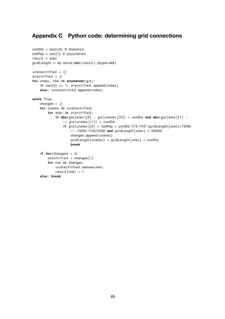
Appendix C Python code: determining grid connections

conDis = zcon [ 0 ] # distanceconPop = con [ 1 ] # populat ionr e s u l t = e lecgr idLength = np . zeros ( len ( r e s u l t ) , dtype= i n t )

u n e l e c t r i f i e d = [ ]e l e c t r i f i e d = [ ]for index , row in enumerate ( g i s ) :

i f row [ 3 ] == 1: e l e c t r i f i e d . append ( index )else : u n e l e c t r i f i e d . append ( index )

while True :changes = [ ]for unelec in u n e l e c t r i f i e d :

for elec in e l e c t r i f i e d :i f abs ( g i s [ e lec ] [ 0 ] - g is [ unelec ] [ 0 ] ) < conDis and abs ( g i s [ e lec ] [ 1 ] -

↪→ g is [ unelec ] [ 1 ] ) < conDis :i f g is [ unelec ] [ 2 ] > conPop + conDis * ( 1 5 . 7 02 * ( gr idLength [ e lec ]+7006)

↪→ /1000 -110) /4400 and gr idLength [ e lec ] < 50000:changes . append ( unelec )gr idLength [ unelec ] = gr idLength [ e lec ] + conDisbreak

i f len ( changes ) > 0 :e l e c t r i f i e d = changes [ : ]for row in changes :

u n e l e c t r i f i e d . remove ( row )r e s u l t [ row ] = 1

else : break

48