Embed Size (px)
Citation preview

ACKNOWLEDGEMENTS
First of all I would like to thank my Supervisors Prof. Dr. Joao Tiago Mexia and
Prof. Dr. Hab. Roman Zmyslony for their friendship, support and trust in me.
To my Friends and Colleagues in the Centre of Mathematics and Applications
of the Nova University of Lisbon. Their opinions, suggestions and friendship were
crucial for this work.
Last, but certainly not least, I thank my Family and Friends for their indefati-
gable support. Without them nothing in my life would be possible.

ii

ABSTRACT
This thesis focuses on inference and hypothesis testing for parameters in orthogonal
mixed linear models. A canonical form for such models is obtained using the matri-
ces in principal basis of the commutative Jordan algebra associated to the model.
UMVUE are derived and used for hypothesis tests. When usual F tests are not
possible to use, generalized F tests arise, and the distribution for the statistic of
such tests is obtained under some mild conditions. application of these results is
made to cross-nested models.

iv

SINOPSE
Esta tese centra-se na inferencia e teste de hipoteses para parametros em modelos
lineares mistos ortogonais. E obtida uma forma canonica para estes modelos usando
as matrizes da base principal da algebra de Jordan comutativa associada ao modelo.
Sao derivados UMVUE que sao usados em testes de hipoteses. Quando nao e possıvel
usar os testes F usuais, surgem os testes F generalizados, e e obtida a distribuicao da
estatıstica destes testes sob algumas condicoes. Estes resultados sao depois aplicados
a modelos com cruzamento-encaixe.

vi

NOTATION INDEX
• X′ : transpose of matrix X
• In : identity matrix of size n
• 0n×m : null matrix of size n×m
• R(X) : linear space spanned by the column vectors of matrix X
• N(X) : kernel of matrix X
• ⊥ : orthogonal
• ⊕ : direct sum of subspaces
• ⊞ : direct sum orthogonal of subspaces
• P[·] : probability
• E[X] : expectation of the random vector X
• V[X] : covariance matrix of the random vector X
• N (µ,V) : normal random vector with mean vector x and covariance matrix
V
• χ2(n) : chi square random variable with n degrees of freedom
• ℓ(t, θ) : loss function of estimate t for θ

• Rθ(T) : risk function of estimator T for θ
• βφ(θ) : power function of test φ on θ
viii
CONTENTS
1. Introduction . . . . . . . . . . . . . . . . . . . . . . . . . . . . . . . . . . . 1
2. Algebraic Results . . . . . . . . . . . . . . . . . . . . . . . . . . . . . . . . 3
2.1 Projection Matrices . . . . . . . . . . . . . . . . . . . . . . . . . . . . 3
2.2 Generalized Inverses . . . . . . . . . . . . . . . . . . . . . . . . . . . 7
2.3 Jordan Algebras . . . . . . . . . . . . . . . . . . . . . . . . . . . . . . 15
3. Inference . . . . . . . . . . . . . . . . . . . . . . . . . . . . . . . . . . . . . 23
3.1 Estimators . . . . . . . . . . . . . . . . . . . . . . . . . . . . . . . . . 23
3.2 Exponential Family of Densities . . . . . . . . . . . . . . . . . . . . . 31
3.3 Estimation on Linear Models . . . . . . . . . . . . . . . . . . . . . . 33
3.3.1 Linear Models . . . . . . . . . . . . . . . . . . . . . . . . . . . 33
3.3.2 Model Structure . . . . . . . . . . . . . . . . . . . . . . . . . . 35
3.3.3 Fixed Effects . . . . . . . . . . . . . . . . . . . . . . . . . . . 37
3.3.4 Variance Components . . . . . . . . . . . . . . . . . . . . . . 40
4. Hypothesis Testing . . . . . . . . . . . . . . . . . . . . . . . . . . . . . . . 49
4.1 Hypothesis Tests . . . . . . . . . . . . . . . . . . . . . . . . . . . . . 49
4.2 Linear Models and F Tests . . . . . . . . . . . . . . . . . . . . . . . . 58
4.3 Generalized F Distribution . . . . . . . . . . . . . . . . . . . . . . . . 62
5. Cross Nested Models . . . . . . . . . . . . . . . . . . . . . . . . . . . . . . 71
5.1 Models . . . . . . . . . . . . . . . . . . . . . . . . . . . . . . . . . . . 71

5.2 Estimators . . . . . . . . . . . . . . . . . . . . . . . . . . . . . . . . . 77
5.3 Hypothesis testing . . . . . . . . . . . . . . . . . . . . . . . . . . . . 81
5.3.1 F Tests . . . . . . . . . . . . . . . . . . . . . . . . . . . . . . 81
5.3.2 Generalized F Tests . . . . . . . . . . . . . . . . . . . . . . . 82
6. Final Remarks . . . . . . . . . . . . . . . . . . . . . . . . . . . . . . . . . 89
x

LIST OF FIGURES
2.1 Subspaces M and L, and the matriz N . . . . . . . . . . . . . . . . . 13
5.1 Acceptance and Rejection Regions . . . . . . . . . . . . . . . . . . . . 83
5.2 Critical Value . . . . . . . . . . . . . . . . . . . . . . . . . . . . . . . 85

xii

1. INTRODUCTION
This work is an attempt to solve some unanswered questions in hypothesis tests
for linear mixed models. It is a very well known fact that in a three way ANOVA
random model the nullity of variance components associated to the main effects can
not be tested with an F test. Several alternatives have been suggested (see [7])
like Bartlett-Scheffe tests and the Satterthwaite’s approximation, but they either
loose information or are too unprecise when the sample is not large enough. So,
under some mild conditions, an exact distribution for such hypothesis is derived.
A characterization of the algebraic structure of linear models is established using
commutative Jordan algebras, like in [22], [25] and [34]. This allows the expression
for the model in a canonical form, which allows the immediate derivation of sufficient
statistics (with normality) and F tests (also assuming normality).
Chapter 2 covers many topics in linear algebra and matrix theory essential in
the analysis and inference for linear models. Special attention is directed to Jordan
algebras, introduced in [6], and commutative Jordan algebras. Regarding the latter,
very important results obtained in [22] and more where presented in [18], [15] and
[11].
Chapter 3 deals with estimation. Firstly, general definitions of estimators and
their properties are given as well as the properties of the exponential family of
distributions, mainly for completeness sake. Definitions of linear models and their
special types are given, like Gauss-Markov models and COBS models, which provide
the foundations to necessary and sufficient conditions for the existence of sufficient
2 1. Introduction
and complete sufficient statistics, both for estimable functions of fixed effects and
variance components (see [25] and [34]). A canonical form for orthogonal models
based on the principal basis of the commutative Jordan algebra is then presented
(see [4]). From a model expressed in this form it is easy to derive complete sufficient
statistics for the parameters in the model.
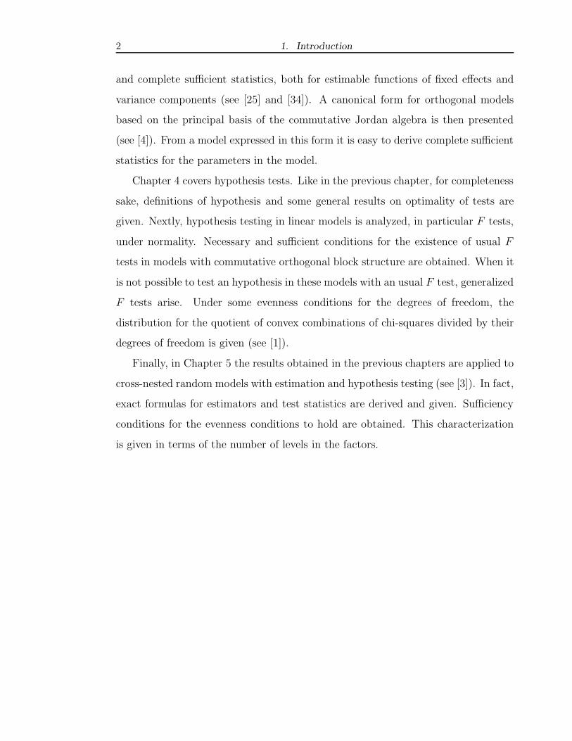
Chapter 4 covers hypothesis tests. Like in the previous chapter, for completeness
sake, definitions of hypothesis and some general results on optimality of tests are
given. Nextly, hypothesis testing in linear models is analyzed, in particular F tests,
under normality. Necessary and sufficient conditions for the existence of usual F
tests in models with commutative orthogonal block structure are obtained. When it
is not possible to test an hypothesis in these models with an usual F test, generalized
F tests arise. Under some evenness conditions for the degrees of freedom, the
distribution for the quotient of convex combinations of chi-squares divided by their
degrees of freedom is given (see [1]).
Finally, in Chapter 5 the results obtained in the previous chapters are applied to
cross-nested random models with estimation and hypothesis testing (see [3]). In fact,
exact formulas for estimators and test statistics are derived and given. Sufficiency
conditions for the evenness conditions to hold are obtained. This characterization
is given in terms of the number of levels in the factors.

2. ALGEBRAIC RESULTS
In this chapter, some elementary and not so elementary results on Matrix Theory
will be presented. Most of these results are proven in readily available literature.
The first part will be a brief discussion of orthogonal projection matrices, followed by
a section on generalized inverses. Lastly, a section on Jordan algebras (or quadratic
subspaces) will introduce some important results that are used in linear models.
2.1 Projection Matrices
Let E be a linear space, and S ⊂ E a linear subspace of E . Let also e1, ..., en be
an orthonormal base for E and e1, ..., er, r < n, be an orthonormal base for S.
With x ∈ E ,
x =r∑
i=1
αiei +n∑
i=r+1
αiei.
Consider now the matrix
E = [E1 E2], (2.1)
with
E1 = [e1 · · · er] and E2 = [er+1 · · · en]. (2.2)
It is then clear that, with α = [α1 · · · αn]′, α1 = [α1 · · · αr]′ and α2 =
[αr+1 · · · αn]′,
x = Eα = E1α1 + E2α2. (2.3)

4 2. Algebraic Results
Due to orthonormality,
E′1E1 = Ir
E′2E2 = In−r
E′1E2 = 0r,n−r
E′2E1 = 0n−r,r
, (2.4)
so that, with Eα1 = u,
E1E′1x = E1E
′1Eα
= E1E′1[E1 E2]
α1
α2
= [E1 0n−r]
α1
α2
= E1α1 = u
(2.5)
So, the projection of a vector on a subspace can be defined:
Definition 1. The vector u described above is called the orthogonal projection of x
in S.
Nextly comes
Theorem 1. Suppose the columns of matrix E form an orthonormal basis for linear
subspace S. Then
PSx = EE′x = u
is the orthogonal projection of x on S.
Proof. See [18], pg. 53.
Thus, follows the natural definition of orthogonal projection matrix.
Definition 2. The matrix PS is called the orthogonal projection matrix on S.

2.1. Projection Matrices 5
Obviously,
R(PS) = SN(PS) = S⊥
. (2.6)
Obtaining the orthogonal projection matrix for the orthogonal complement of S is
immediate, since, using previous notation,
(In − E1E′1)x = x −E1α1 = E2α2 = v. (2.7)
The next theorem shows that the choice of the orthonormal basis for a subspace
is independent of the orthogonal projection matrix, rendering it unique.
Theorem 2. Suppose the columns of each matrix, E and D, form an orthonormal
basis for linear subspace S. Then
EE′ = DD′.
Proof. See [18], pg. 53.
It is easy to see that PS = E1E′1 is symmetric,
P′S = (E1E
′1)
′ = E1E′1 = PS ,
and idempotent,
PSPS = E1E′1E1E
′1 = E1IrE
′1 = E1E
′1 = PS .
The next theorem shows the converse.
Theorem 3. Every symmetric and idempotent matrix P is an orthogonal projection
matrix.
Proof. See [18], pg. 59.
The following lemma enumerates equivalent statements about orthogonal pro-
jection matrices and associated subspaces.
6 2. Algebraic Results
Lemma 1. The following propositions are equivalent:
1. P is an orthogonal projection matrix;
2. In − P is an orthogonal projection matrix;
3. R(P) = N(In − P);
4. R(In − P) = N(P);
5. R(P)⊥R(In − P);
6. N(P)⊥N(In − P).
The direct sum of linear subspaces can also be represented by the range space of
orthogonal projection matrices. In this case, the direct sum of orthogonal subspaces
is represented by ⊞. The two following theorems show this.
Theorem 4. Let P1, ...,Pk be orthogonal projection matrices such that PiPj = 0n
when i 6= j. Then:
1. P =∑k
i=1 Pi is an orthogonal projection matrix;
2. R(Pi) ∩ R(Pj) = 0 when i 6= j;
3. R(P) =⊕k
i=1 R(Pi).
Proof. See [15], pgs. 241–242.
Theorem 5. Let P be an orthogonal projection matrix associated with a linear
subspace S. Suppose that S is a direct sum of subspaces, i.e., S =⊕k
i=1 Si. Then
there exist unique projectors P1, ...,Pk such that P =∑k
i=1 Pi and PiPj = 0n×n
when i 6= j.
Proof. See [15], pg. 242.

2.2. Generalized Inverses 7
It is interesting to observe that the last two theorems are the reverse of each
other
Another simple way to obtain the orthogonal projection matrix of the column
space, R(X), of a full rank matrix is (see [15], pg. 243) to consider:
PR(X) = X(X′X)−1X′. (2.8)
2.2 Generalized Inverses
Generalized inverses are a very versatile tool, both in linear algebra, as well as in
statistics. Generalized inverses can be derived from two different contexts: equation
systems and linear applications.
From the first point of view, let
Ax = y
be a system of linear equations. If A is invertible, the solution will be x = A−1y. If
A is not invertible, there may still be a matrix G such that x = Gy is a solution for
the system, for every y, whenever the system is consistent. Such a matrix is called
a generalized inverse of A.
The other point of view, which will be followed throughout the dissertation, takes
matrices as linear applications. The adopted definition of generalized inverse will be
based on this.
Definition 3. Let A ∈ Mn×m. A matrix G ∈ Mm×n such that
AGA = A
is called a generalized inverse ( g-inverse) of A, and it is expressed as A−.
The problem that arises naturally is the question of existence: is there a g-inverse
for every matrix? The answer is given by the next theorem.

8 2. Algebraic Results
Theorem 6. For every A ∈ Mn×m, A− ∈ Mm×n exists.
Proof. See [15], pg. 266.
Introducing some useful properties on generalized inverses:
Theorem 7. Let A ∈ Mn×m. Then:
1. (A−)′is a g-inverse of A′;
2. with α 6= 0, α−1A− is a g-inverse of αA;
3. if A is square and non-singular, A− = A−1 uniquely;
4. B and C are non-singular, C−1A−B−1 is a g-inverse of BAC;
5. rank(A) = rank(AA−) = rank(A−A) ≤ rank(A−);
6. rank(A) = n⇔ AA− = In;
7. rank(A) = m⇔ A−A = Im;
8. AA− is idempotent.
Proof. Properties 1 through 7 are proved in [18], pg. 194. As for property 8,
AA−AA− = (AA−A)A− = A.
For a given matrix, as shown before, there exists at least one g-inverse, but
uniqueness doesn’t certainly hold. Thus, a definition of g-inverse class is required.
Definition 4. The set of all g-inverses of A is called the class of g-inverses of A,
and it is denoted by A−.
The next theorem characterizes the elements in A−.

2.2. Generalized Inverses 9
Theorem 8. Let G be a g-inverse of A ∈ Mn×m. Then, any g-inverse of A has
one of the following forms:
1. A− = G + U − GAUAG, for some U ∈ Mm×n;
2. A− = G+V(In−AG)−(Im−GA)W, for some V ∈ Mm×n and W ∈ Mm×n.
Proof. See [15], pg. 277.
By this result, the whole class of g-inverses of A, A−, is obtained from one of
it’s members. Conversely, the class of g-inverses identifies the original matrix, since
Theorem 9. Let A and B be two matrices such that A− = B−. Then A = B.
Proof. See [15], pgs. 277–278.
But is there any sort of invariance when computing with such matrices? The
important results that follow show that there is.
Theorem 10. Let A ∈ Mn×m, B ∈ Mp×n and C ∈ Mm×q be matrices such that
R(B′) ⊆ R(A′) and R(C) ⊆ R(A). Then BG1C = BG2C for all G1,G2 ∈ A−.
Proof. See [15], pg. 268.
As a consequence, the following corollary arises.
Corollary 1. A(A′A)−(A′A) = A and (A′A)−(A′A)A′ = A′.
Proof. In [15], pg. 268, this corollary is proved for matrices with complex elements
which includes matrices with real elements.
The following results connect g-inverses with orthogonal projection matrices.
Theorem 11. Let A ∈ Mn×m. Then A(A′A)−A′ is the orthogonal projection
matrix of R(A).

10 2. Algebraic Results
Proof. If A is a real matrix then (see [15], in pg. 269) A(A′A)−A′ is symmetric
and idempotent. Therefore, A(A′A)−A′ is an orthogonal projection matrix. It is
obvious that
R(A(A′A)−A′
)⊆ R(A) .
Since A = A(A′A)−A′A,
R(A) = R(A(A′A)−A′A
)⊆ R
(A(A′A)−A′
),
and hence, R(A) = R(A(A′A)−A′), which proves that A(A′A)−A′ is the orthogo-
nal projection matrix of R(A).
The g-inverse is the less restrictive case of the generalized inverse. Particularly,
A− being a g-inverse of A does not imply that A is a g-inverse of A−. When this
happens, A− is called a reflexive g-inverse.
Definition 5. Let A ∈ Mn×m and G ∈ Mm×n. When AGA = A and GAG = G,
G is called a reflexive g-inverse. Such a matrix is denoted by A−r .
The real interesting fact that characterizes reflexive g-inverses is that, while
in a general g-inverse rank(A) ≤ rank(A−), for a reflexive g-inverse rank(A) =
rank(A−r ), as stated in
Theorem 12. Let A ∈ Mn×m. G ∈ Mm×n is a reflexive g-inverse of A if and
only if G is a g-inverse of A and rank(A) = rank(G).
Proof. See [15], pg. 279.
Existence of g-inverses is also guaranteed.
Theorem 13. For each A ∈ Mn×m, a reflexive g-inverse exists.
Proof. See [15], pg. 279.
2.2. Generalized Inverses 11
It is interesting to characterize the subspaces associated to a matrix A and it’s
g-inverses. The following theorem enlightens this connection.
Theorem 14. Let A ∈ Mn×m and A− ∈ Mm×n one of it’s g-inverses. Let
N = A− −A−AA−;
M = R(A− − N
)= R
(A−AA−
);
L = N(A− − N
)= N
(A−AA−
).
Then
1. AN = 0n×n and NA = 0m×m;
2. M∩ N(A) = 0 and M⊕ N(A) = Rm;
3. L ∩ R(A) = 0 and L ⊕ R(A) = Rn.
Proof. Thesis 1 is quite easy to prove since
NA = A−A − A−AA−A = A−A − A−A = 0m×m
and
AN = AA− − AA−AA− = AA− − AA− = 0n×n.
As for thesis 2 and 3, see [15], pgs. 282–283.
Conversely, choosing N, M and L, a g-inverse of A for which the conditions in
the previous theorem hold may be found.
Theorem 15. Let A ∈ Mn×m. Choosing a matrix N ∈ Mm×n such that AN =
0n×n and NA = 0m×m, a subspace L of Rn such that L ∩ R(A) = 0 and L ⊕R(A) = Rn, and a subspace M∩ N(A) = 0 of Rm such that M∩ N(A) = 0and M⊕ N(A) = Rm. Then there exists a g-inverse of A, A−, such that

12 2. Algebraic Results
1. N = A− − A−AA−;
2. M = R(A− − N) = R(A−AA−);
3. L = N(A− − N) = N(A−AA−).
Proof. See [15], pg. 283.
In virtue of the specificity of this construction, a separate definition is in order.
Definition 6. Let A ∈ Mn×m. A matrix for which the assumptions of Theorem 15
hold is called a LMN-inverse.
Uniqueness of LMN-inverses is also guaranteed.
Theorem 16. A LMN-inverse of a matrix A is unique.
Proof. See [15], pg. 284.
The relationship between the subspaces M and L, and the matrix N with the
matrix A is illustrated in the figure
Finally, a bijection between between all triplets (M,L,N) and all g-inverses is
established in
Theorem 17. Let A ∈ Mn×m, and consider L ⊆ Rn, M ⊆ Rm and N ∈ Mm×n as
defined in Theorem 15. Then there exists a bijection between the set of all triplets
(M,L,N) and the set of all g-inverses, A−.
Proof. See [15], pg. 286.
Furthermore, a bijection between all pairs (L,M) and all reflexive g-inverses can
be established.
Theorem 18. Let A ∈ Mn×m, and consider L ⊆ Rn and M ⊆ Rm as defined in
Theorem 15. Then there exists a bijection between the set of all triplets (M,L,N)
and the set of all reflexive g-inverses.

2.2. Generalized Inverses 13
Fig. 2.1: Subspaces M and L, and the matriz N
Proof. See [15], pg. 286.
Another interesting fact is the connection between subspaces L and M, and their
orthogonal projection matrices.
Theorem 19. Let A− be a g-inverse of A. With
• N = A− −A−AA−;
• M = R(A− − N);
• L = N(A− −N);
follows
AA− = PR(A) ∧ A−A = PM ⇔ M⊕ N(A) = Rm ∧ R(A) ⊕ L = Rn.
Proof. Suppose AA− = PR(A). Then, for all y ∈ Rn, y = y1 + y2, with y1 ∈ R(A).
Now, for all y2 = y − y1,
AA−y2 = 0 ⇒ A−AA−y2 = 0 ⇒ (A− −N)y2 = 0.

14 2. Algebraic Results
This means that any element that is linearly independent of R(A) belongs to L.
Suppose now that A−A = PM. Let x ∈ Rm be expressed as x = x1 + x2, with
x1 ∈ M. Then
A−Ax2 = 0 ⇒ AA−Ax2 = 0 ⇒ Ax2 = 0,
which means that any element that is linearly independent of M belongs to N(A− −N).
This shows that AA− = PR(A)∧A−A = PM ⇒ M⊕N(A) = Rm∧R(A)⊕L = Rn.
Suppose now that R(A) ⊕ L = Rn. With y = y1 + y2, y1 ∈ R(A) and y2 ∈ L,
AA−y = AA−y1 + AA−y2 ⇒ (A− − N)y
= (A− −N)y1 + (A− − N)y2
= (A− −N)y1
⇒ AA−y = AA−y1 = AA−Ax
= Ax = y1,
with y1 = Ax. Thus, AA− = PR(A). Now, for all x ∈ Rm, let x = x1 + x2, with
x1 ∈ M and x2 ∈ N(A). Since
A−Ax = A−Ax1 + A−Ax2
= A−Ax1
= A−AA−AA−y
= A−AA−y
= x1,
where x1 = (A− − N)y. Thus A−A = PM, and the proof is complete.
A special type of LMN-inverse is obtained taking N = 0m×m, M = N(A)⊥ and
L = R(A)⊥. This set of conditions is equivalent to the set of conditions
1. G is a reflexive g-inverse of A;
2. AG = PR(A);

2.3. Jordan Algebras 15
3. GA = PR(G).
According to [18], pg. 173 (Theorem 5.2), these conditions are equivalent to having
1. G is a reflexive g-inverse of A;
2. (AG)′ = AG;
3. (GA)′ = GA.
These are the properties that define the Moore-Penrose inverse.
Definition 7. For a matrix A ∈ Mm×n, a matrix G is denominated its Moore-
Penrose inverse if the following hold:
• G is a reflexive g-inverse of A;
• (AG)′ = AG;
• (GA)′ = GA.
2.3 Jordan Algebras
This section is entirely dedicated to the algebraic structures known as Jordan alge-
bras. These structures were first introduced by Pascual Jordan (who named these
algebras), John von Neumann and Eugene P. Wigner in quantum theory, as an alter-
native algebraic structure for quantum mechanics. In this section Jordan algebras
will be defined and their properties explored.
For completeness sake, the definition of algebras is stated.
Definition 8. An algebra A is a linear space equipped with a binary operation ∗,usually denominated product, in which the following properties hold for all α ∈ R
and a,b, c ∈ A:

16 2. Algebraic Results
• a ∗ (b + c) = a ∗ b + a ∗ c;
• (a + b) ∗ c = a ∗ c + b ∗ c;
• α(a ∗ b) = (αa) ∗ b = a ∗ (αb).
It is important to underline that associativity and commutativity are properties
that are not necessary for a linear space to be an algebra. The definitions follow.
Definition 9. An algebra A is associative if and only if, for all a,b, c ∈ A,
(a ∗ b) ∗ c = a ∗ (b ∗ c).
Definition 10. An algebra A is commutative if and only if, for all a,b ∈ A,
a ∗ b = b ∗ a.
As for all algebraic structures, substructures are obtained, in this case easily.
Definition 11. A set S contained in an algebra A is a subalgebra if it is a linear
subspace and if
∀a,b ∈ S : a ∗ b ∈ S.
In order to define a Jordan algebra, one needs to define the Jordan product in
an algebra.
Definition 12. A Jordan product is a binary operation · defined on an algebra Afor which the following two conditions, a,b ∈ A:
• a · b = b · a;
• a2· · (b · a) = (a2· · b) · a,
with a2· = a · a, hold. An algebra equipped with such a product is a Jordan algebra.

2.3. Jordan Algebras 17
This is the primary definition for a Jordan algebra. Other more intuitive and
tractable equivalent definitions will follow. A Jordan subalgebra is equally defined.
Definition 13. A set S contained in a Jordan algebra A is a Jordan subalgebra if
it is a linear subalgebra of the algebra A and if
∀a,b ∈ S : a · b ∈ S.
Again, more natural definitions of Jordan subalgebras will be presented.
For illustration purposes, consider an example of a Jordan algebra. Let Sn be
the space of symmetric real matrices of size n. It is a linear space with dimension
n(n+1)2
, equipped with the (associative) matrix product. If the · product is defined
as
A ·B =1
2(AB + BA), (2.9)
it is quite easy to see that the · product is a Jordan product in Sn, and Sn is in fact
a Jordan algebra. This is a very important instance of Jordan algebras, since it is
the space in which covariance matrices lie. In order to show the importance of this
Jordan algebra, some definitions must be given first.
Definition 14. Algebra A is algebra-isomorphic to algebra B if and only if there
exists a bijection φ : A 7→ B such that, for all α, β ∈ R and a,b ∈ A,
1. φ(αa + βb) = αφ(a) + βφ(b);
2. φ(a ∗ b) = φ(a) ∗ φ(b).
With algebra-isomorphism it is then possible to identify special Jordan algebras.
Definition 15. A Jordan algebra algebra-isomorphic to a subalgebra of Sn is de-
nominated a special Jordan algebra.

18 2. Algebraic Results
Matrix algebras are the fulcral application of Jordan algebras in statistics. Most
of the following results are presented in the context of such spaces. Nextly, identity
elements and idempotent elements are formally defined.
Definition 16. Let E ∈ S, S a subspace of Mn. The element E is an associative
identity element if ES = SE = S, ∀S ∈ S.
It is important to remember that, with S being a subset of Mn, the identity
element is not necessarily In.
Definition 17. Let E ∈ Mn. If E2 = E, E is said to be idempotent.
Here, it is also important to refer that if an element is idempotent, it is also
Jordan idempotent: E2· = E. A similar result is obtained for Jordan identities:
Theorem 20. Let S be a subspace of Sn and E ∈ S an idempotent element. Then
∃S ∈ S : E · S = E · S ⇒ ES = SE = S.
Proof. See [11], pages 9 and 10.
The next theorem sets the connection between idempotency, orthogonality and
Jordan orthogonality.
Theorem 21. Let S and T be subspaces of Sn. Then the following three conditions
hold:
1. ∀S ∈ S,E · S = S ⇔ ∀S ∈ S,ES = S = SE;
2. with E1 and E2 idempotent elements, E1 · E2 = 0 ⇔ E1E2 = 0;
3. ∀S ∈ S, ∀T ∈ T ,S · T = 0 ⇔ ∀S ∈ S, ∀T ∈ T ,ST = TS = 0.
Proof. See [11], page 10.

2.3. Jordan Algebras 19
After these remarks on some properties of Jordan algebras, more standard equiv-
alent definitions of Jordan algebras are presented, included the one in [22].
Theorem 22. Let S be a subspace of Sn with identity element E and A and B any
two elements of S. Then S is a Jordan algebra if and only if any of the following
equivalent definitions hold:
1. AB + BA ∈ S;
2. ABA ∈ S;
3. ABC + CBA ∈ S;
4. A2 ∈ S;
5. A+ ∈ S.
Proof. For the proof of the assertions in this theorem see [6], [22], [32] and [11].
It is easy to see that, by the second and third conditions of the last theorem, any
power of a matrix belonging to a Jordan algebra belongs to that Jordan algebra.
It is interesting to see that one of the definitions of Jordan algebra is based on
the presence of the Moore-Penrose inverse of each matrix in the algebra.
Like in all linear spaces, defining a inner product in Jordan algebras is very im-
portant. Although many functions can qualify as inner products in Jordan algebras,
but one of the most common functions is defined, in S, as
<A|B>= tr(AB′) . (2.10)
Consider now that S, spanned by M1, ...,Ms is included in Sn and let In ∈ S.
Let A(S) be the smallest associative algebra in Mn containing S. Also define
B(S) = B ∈ S : SBS ∈ S, ∀S ∈ S. (2.11)
Given this,

20 2. Algebraic Results
Theorem 23. B(S) is the maximal subspace of S such that
BSB ∈ S, ∀S ∈ S, ∀B ∈ B(S).
Proof. See [11], Chapter 3.
Finally, consider J (S) ⊆ Sn the smallest Jordan algebra containing S.
Theorem 24. Given S, B(S), A(S) and J (S),
B(S) ⊆ S ⊆ J (S) ⊆ A(S) ∩ Sn ⊆ A(S).
Proof. The proof of this theorem can be found on [11], in pages 16 through 18.
It is important to notice that the inclusion J (S) ⊆ A(S)∩Sn is in general strict,
meaning that Jordan algebras generated by sets of symmetric matrices have lower
dimensions than the associative algebra generated by the same set. Equality holds
only when the matrices in the generating set commute, i.e., AB = BA.
On the following paragraphs, emphasis will be given to the decomposition in
partitions of Jordan algebras as linear spaces and conditions given on orthogonality
between matrices contained in such partitions. The section will culminate with the
seminal result by Seely, pointing an unique basis constituted by mutually orthogonal
projection matrices for commutative Jordan algebras. The following definition is
necessary:
Definition 18. Let S =⊗s
i=1 Si ⊆ Sn. For each element A of S, A =∑s
i=1 Ai,
with Ai ∈ Si. The set i ∈ N : Ai 6= 0 is called the support of A.
With this definition in mind, the following results are obtained:
Theorem 25. Let S ⊆ Sn and In ∈ S. Then, for A,B ∈ B(S), the following
propositions are equivalent:
1. SASBS = 0n×n, ∀S ∈ S;

2.3. Jordan Algebras 21
2. ASB = 0n×n;
3. AB(S)B = 0n×n;
4. A and B have disjoint support in B(S).
Proof. See [11], Chapter 3.
Theorem 26. Let S ⊆ Sn and In ∈ S. Then, for A,B ∈ J (S), the following
propositions are equivalent:
1. SASBS = 0n×n, ∀S ∈ J (S);
2. AJ (S)B = 0n×n;
3. A and B have disjoint support in J (S).
Proof. See [11], Chapter 3.
Theorem 27. Let A,B ∈ Sn. Then
ASB = 0n×n ⇔ AJ (S)B = 0n×n.
Proof. See [11], pages 25–26.
Theorem 28. Let S ⊆ Sn and In ∈ S. Then, for A,B ∈ J (S), the following
propositions are equivalent:
1. SASBS = 0n×n, ∀S ∈ S;
2. ASB = 0n×n;
3. AJ (S)B = 0n×n;
4. A and B have disjoint supports in J (S).

22 2. Algebraic Results
Proof. The proof for this theorem follows directly from Theorem 25 and Theorem
26.
The last part of this section is dedicated to the sets of matrices that form basis
for commutative Jordan algebras. First, the existence of a basis is settled.
Theorem 29. For every commutative Jordan algebra there exists at least one basis
Q1, . . . ,Qw
constituted by orthogonal projection matrices such that QiQj = 0n×n, for i 6= j.
Proof. See [22], in which one may find an algorithm for the construction of this
basis.
Theorem 30 (Seely, 1971). A necessary and sufficient condition for a subspace S ⊆Sn to be a commutative Jordan algebra is the existence of a basis Q1, ...,Qs formed
by orthogonal projection matrices, such that QiQj = 0n×n, for i 6= j, i, j = 1, ..., s.
Furthermore, this basis is unique.
Proof. The existence was proven in Theorem 29. As for the uniqueness, consider
another basis formed by orthogonal projection matrices, P1, ...,Ps. Hence, for
j = 1, ..., s,
Pj =
s∑
i=1
αiQi and Qi =
s∑
j=1
βi,jPj,
with the coefficients αi and βi,j, i, j = 1, ..., s, being unique and equal to 0 or 1, since
the matrices Pj and Qi, i, j = 1, ..., s, are orthogonal projection matrices. Thus,
choosing j,
Pj = βi,jPj = QiPj = αiQi = Qi,
for some i. Since this holds for all j = 1, ..., s, the proof is complete.

3. INFERENCE
In this chapter the discussion will be focused on the estimation of parameters and
functions of parameters of linear models, namely fixed effects, variance components
and functions of fixed effects and variance components.
Estimators, in a broad sense, will be presented as well as their properties. Nextly,
estimators for parameters and functions of parameters in linear models will be pre-
sented and their properties discussed.
3.1 Estimators
In order to define an estimator for any given parameter, one needs to retrieve in-
formation from a (finite) sample. Usually a function of the observations vector is
taken – a statistic or estimator – in order to accomplish this mission.
It is desirable, of course, that statistics contain as much information about the
parameter as possible. A usual condition is that the statistic is sufficient. The
definition follows.
Definition 19. Given the sample vector X = (X1, ..., Xn)′ where each component
has its probability density belonging to a family of densities P = fθ(·) : θ ∈ Ω,the function T(X) = T(X1, ..., Xn) is a sufficient statistic if the sampled density
fθ(·) ∈ P, given T(X) = t, does not depend on θ.
This definition guarantees that a sufficient statistic summarizes all the informa-
tion contained in a sample about parameter θ, but it becomes quite intractable

24 3. Inference
to establish this property. Usually the following theorem is used as a sufficiency
criterium.
Theorem 31 (Factorization Criterion). T(x) is a sufficient statistic to θ if and
only if
fθ(x) = gθ
(T(x)
)h(x).
Proof. See [9], pp. 54 and 55.
Sufficiency does in fact guarantee that all the necessary information is retrieved
from a sample, but it doesn’t stop one from shooting a fly with a cannon. Many
sufficient statistics exist for a given sample from a population with density fθ – from
a vector of sample observations functions to even a single one – and it is desirable
to have a statistic as condensed as possible, since for every set of distributions, the
whole sample is sufficient. To aid in such a goal, the concept of minimal sufficient
statistics is introduced:
Definition 20. A sufficient statistic T is minimal if for all sufficient statistic U
there exists a function g such that T = g(U).
Besides this, there are statistics that do not carry any kind of information about
the parameter, although they do carry information about the sample itself. These
are called ancillary statistics, and they are valuable to determine the amount of
“useless” information carried by a statistic. The definition:
Definition 21. A statistic V is called ancillary if its distribution is independent of
the parameter θ.
Opposite to this definition is completeness, which says that a sufficient statistic
doesn’t carry useless – ancillary – information. Formally,
Definition 22. A statistic T is complete if and only if
E[g (T)] = 0, ∀θ ∈ Ω ⇒ P[g ≡ 0] = 1.

3.1. Estimators 25
It is, thus, fair to assume that a complete statistic is independent of any ancillary
information. This is stated in the next theorem.
Theorem 32 (Basu’s Theorem). Given θ, if T is a complete sufficient statistic
then any ancillary statistic V is independent of T.
Proof. See [10], pg. 42.
Another expected fact is that every complete sufficient statistic is a minimal
sufficient statistic.
Theorem 33. If a statistic T is complete sufficient then it is is minimal sufficient.
Proof. See [17].
It is necessary to have some kind of efficiency measure for estimators. First,
define the loss function.
Definition 23. Let T be an estimator of g(θ). The real-valued function ℓ(t, θ) is
a loss function if it respects the following conditions:
1. ℓ(t, θ) ≥ 0;
2. ℓ(g(θ), θ
)= 0.
This function assigns a penalization to an estimate obtained by T different of
g(θ). But of course that the loss isn’t known, so, one must find a way to assess the
average loss: this is accomplished using the risk function.
Definition 24. Let T be an estimator of g(θ) and ℓ(t, θ) its loss function. The
risk function is defined as
Rθ(T) = E[ℓ(T, θ)] .

26 3. Inference
It also provides an order relationship between estimators. So,
T1 ≺ T2 if ∀θ ∈ Ω,Rθ(T1) ≤ Rθ(T2) ∧ ∃θ ∈ Ω : Rθ(T1) < Rθ(T2). (3.1)
From this ordering of estimators comes the definition of admissibility.
Definition 25. An estimator T is admissible if there exists no estimator U such
that U ≺ T.
Given the definition of risk and sufficiency, it is possible to enunciate an im-
portant theorem that permits the improvement of an estimator not built upon a
sufficient statistic: the Rao-Blackwell theorem.
Theorem 34 (Rao-Blackwell Theorem). Given an estimator U of g(θ) with a loss
function ℓ(u, θ) strictly convex on u and such that
• E[U] <∞;
• Rθ(U) <∞;
and a sufficient statistic T, then f(T) = E[U | T] verifies
Rθ(U) ≥ Rθ
(f(T)
),
with the equality holding if and only if
P[U ≡ f(T)] = 1.
Proof. See [10], pg. 48.
The concept of information, in what statistics are concerned, as well as the
amount of it the estimator carries can be interpreted using what it is called the
information matrix :

3.1. Estimators 27
Definition 26. Let X = (X1, ..., Xn)′ be a sample vector belonging to the family
P = fθ(·) : θ ∈ Ω of densities, with θ = (θ1, ..., θs)′, and let T be a statistic. The
element Iij(θ) of the information matrix I(θ) is defined as
Iij(θ) = E
[∂
∂θi
log(fθ(X)
)· ∂
∂θj
log(fθ(X)
)].
This matrix measures the variation ratio of the density fθ with θ, thus informing
the change on the value of θ. It is then possible, with this concept, to obtain a bound
for the variance of an estimator:
Theorem 35. Let X be a sample vector belonging to a family P = fθ(·) : θ ∈ Ω,with θ = (θ1, ..., θs)
′, in which Ω is an open set and densities fθ(·) have a common
support, and T a statistic such that E[T 2] <∞. Let one of the following conditions
hold:
• ∂∂θi
E[T ] = E[
∂∂θiT]
exists ∀i = 1, ..., s;
• There exist functions bθ,i(·), i = 1, ..., s, with E[b2θ,i(X)
]<∞, such that ∀∆ >
0 :
∣∣∣∣fθ+∆εi
(x) − fθ(x)
∆
∣∣∣∣ < bθ,i(x), i = 1, ..., s.
Then E[
∂∂θi
log(fθ(X)
)]and
V[T ] ≥ α′(I(θ)
)−1α,
with αi = ∂∂θi
E[T ], i = 1, ..., s.
Proof. See [10], p. 127.
The discussion will now be restricted to unidimensional parameters and unidi-
mensional functions of the same parameter. The next step would be to find es-
timators with optimal properties. But in fact, the class of all estimators is too
large and general to derive such an estimator, even with the adequate optimality
criteria. To surround this problem, it is now introduced a criterion which restricts

28 3. Inference
the estimator’s space and gives the estimators a desirable property: unbiasedness.
Formally,
Definition 27. An estimator T for a parameter θ ∈ Ω is unbiased if
E[T ] = θ, ∀θ ∈ Ω.
Functions g(θ) and parameters θ for which there exist unbiased estimators are
called estimable functions and parameters, respectively. Finding the best estimator
in this class may be somewhat difficult, and characterizing all unbiased estimators
is a very useful achievement. This is shown in
Lemma 2. Let T be an unbiased estimator of g(θ). Every unbiased estimator U of
g(θ) has the form
U = T − T0,
where T0 is an unbiased estimator of 0.
Proof. It is quite simple, because
E[U ] = E[T ] − E[T0] = g(θ). (3.2)
Another interesting fact is the uniqueness of unbiased estimators given a complete
sufficient statistic.
Lemma 3. Let g(θ) be an estimable function and T a complete sufficient statistic.
If f and h are functions such that
E[f(T )] = E[h(T )] = g(θ),
then
P[f ≡ h] = 1.
3.1. Estimators 29
Proof. See [10], pp. 87–88.
Nextly, a widely used optimality criterion is defined: uniformly minimum vari-
ance unbiased estimation. The definition follows:
Definition 28 (UMVUE). An estimator T of g(θ) is an UMVUE (Uniformly Min-
imum Variance Unbiased Estimator) if
1. E[T ] = g(θ);
2. V[T ] ≤ V[U ], where U is an unbiased estimator of g(θ).
The class of all unbiased estimators of 0 is an important class in what regards to
UMVUEs. In fact this class distinguishes UMVUEs apart from other less effective
estimators. This is brought by
Theorem 36. Let T be an unbiased estimator of g(θ) such that E[T 2] < ∞. T is
an UMVUE of g(θ) if and only if
Cov[T, U ] = 0, U ∈ U
with U ∈ U , the class of all unbiased estimators of 0.
Proof. See [10], pg. 86.
It is also possible to refine the Rao-Blackwell theorem:
Theorem 37. Given an unbiased estimator U of g(θ) with a loss function ℓ(u, θ)
strictly convex on u and such that
• E[U ] <∞;
• Rθ(U) <∞;
and a sufficient statistic T , then f(T ) = E[U | T ] verifies

30 3. Inference
• E[f(T )] = g(θ);
• Rθ(U) ≤ Rθ
(f(T )
);
with the equality holding if and only if
P[U ≡ f(T )] = 1.
Proof. See [14], pg. 322.
The relationship between completeness of statistics and UMVUEs helps to pro-
vide estimators with optimal properties as long as ancillary information is disposed
of. This is the core of
Theorem 38. Let X be a random vector with density fθ and let
E[S] = g(θ).
Let also T be a complete sufficient statistic. Then there exists a function f such that
f(T) is an UMVUE of g(θ). Furthermore, this function is unique with probability
1.
Proof. This theorem is adapted from theorem 1.11 in [10], taking
ℓθ(u) =(u− g(θ)
)2
and, consequently, the risk of S to be
Rθ(S) = E[ℓθ(S)] = E[(S − g(θ)
)2].
When S is unbiased
Rθ(S) = E[(S − E[S]
)2]= V[S] .
A more generalized version of this theorem can be found in [10], pg. 88, and it is
the consequence of lemma 1.10 and the discussion in the precedent pages.

3.2. Exponential Family of Densities 31
3.2 Exponential Family of Densities
Up until now, inference on unknown parameters was made without any kind of
restrictions on the family of distributions underlying in the model. Restricting the
type of distributions may in fact narrow the scope of applications but it can lead
to stronger and more useful results. This section will verse on a specific family of
densities: the exponential family of densities.
Definition 29. A density fθ(·) belongs to the s-dimensional exponential family if it
can be expressed in the form
fθ(x) = h(x) exp
(s∑
i=1
ηiTi(x) − a(η)
).
The η = η(θ) are known as the natural parameters of the density. The natural
parameter space will be denoted by Ξ.
Another consequence of the specification of this family of distributions is the
easy derivation of the cumulants and, consequently, of the moments of a random
variable of the exponential family.
Theorem 39. Let X be a random vector with density belonging to the exponential
family. Then, for each Ti, i = 1, ..., s, the moment generating function
MTi(u) = ea(η+u)−a(η)
and the cumulant generating function
KTi(u) = a(η + u) − a(η)
are defined in some neighborhood of 0.
Proof. See [10], pgs. 27–28.

32 3. Inference
Statistics T1, ..., Ts are in fact very important. It is easy to see that, due to
the factorization criterion (theorem 31) these statistics will be sufficient. Another
important fact is linear independence between the Ti, i = 1, ..., s, and linear inde-
pendence between parameters ηi, i = 1, ..., s. Thus the following
Definition 30. A density belonging to the exponential family is said to be of full
rank if the Ti, i = 1, ..., w, are linearly independent, the ηi, i = 1, ..., s, are linearly
independent and if Ξ contains a s-dimensional rectangle.
It is clear that the Ti, i = 1, ..., s, are sufficient statistics but, in the exponential
family case they are also minimal, as shown in
Theorem 40. Let Ξ ⊆ Rs and X be a random vector belonging to the exponential
family. If the density is of full rank or if the parameter space Ξ contains a set of
points that generate Rs and do not belong to a proper affine subspace of Rs, statistics
T1, ..., Ts are minimal sufficient.
Proof. See [10], pg. 39.
Completeness is also achieved in this family of densities.
Theorem 41. Let X be a random vector with density belonging to the exponential
family with full rank. Then the statistics Ti, i = 1, ..., s, are complete.
Proof. See [9], pgs. 142–143.
An interesting property of this family of densities is connected with the informa-
tion matrix of an estimator for the parameter vector.
Theorem 42. Let X be a random vector with density belonging to the s-dimensional
exponential family, and let also
E[Ti] = τi, i = 1, ..., s.
Then I(τ ) = (V[T])−1, with τ = (τ1, ..., τs)′ and T = (T1, ..., Ts)
′.

3.3. Estimation on Linear Models 33
Proof. See [10], pg. 136.
One of the most important results connected to the exponential family of distri-
butions is that any unbiased estimator which is a function of the T1, ..., Ts will be
an UMVUE.
Theorem 43 (Blackwell-Lehmann-Scheffe Theorem). Let X be a random variable
with density belonging to the exponential family, of full rank and parameter θ. For
any unbiasedly estimable function g(θ) there exists an UMVUE that is a function
of T. Furthermore, it is unique.
Proof. The thesis is a direct consequence of theorem 38 and of theorems 40 and
41.
3.3 Estimation on Linear Models
In this section linear models of various types will be discussed, along with the tech-
niques for estimation of parameters, both fixed and random. The most common and
important models are described, followed by fixed effects estimation theory, which
is fairly established. Lastly, variance components estimation is covered.
3.3.1 Linear Models
A random variable described by a linear model has the structure
y = Xβ. (3.3)
or, rewriting, it can be the sum of several terms:
y =
w∑
i=1
Xiβi. (3.4)
Parameters βi (or β) are fixed unknown variables or random variables. It is on this
last feature that come the first characterizations of linear models.
34 3. Inference
Definition 31. A linear model
y =
b∑
i=1
Xiβi + e,
where matrices Xi, i = 1, . . . , b, are known, vectors βi, i = 1, . . . , b, are fixed and
unknown and e is a random vector with null mean vector and covariance matrix
σ2V, with V a known matrix and σ2 unknown, is said to be a fixed effects model.
This is the most widespread model in applications, both in analysis of variance
as well in linear regression models.
In order to acquaint with random effects, one can consider models with param-
eters that are random variables, besides the usual error.
Definition 32. A linear model
y = 1µ+
w∑
i=1
ei,
where µ is fixed and unknown and e1, . . . , ew are random with null mean vectors
and covariance matrices σ21V1, . . . , σ
2wVw, with V1, . . . ,Vw known, is said to be a
random effects model.
This model is usually applied to the analysis of variance of random effects.
Following the definition of these two models, there is, of course, the mixed model:
Definition 33. A linear model
y =
b∑
i=1
Xiβi +
w∑
i=b+1
ei,
with b < w, β1, . . . ,βb fixed and unknown and e1, . . . , ew are random vectors with
null mean is said to be a mixed effects model.
These are the models in which this work will verse on and, in fact, both fixed
and random effects models are particular cases of the mixed effects model.

3.3. Estimation on Linear Models 35
3.3.2 Model Structure
A particular case of the fixed effects model is the
Definition 34 (Gauss-Markov Model). A fixed effects model
y =
w∑
i=1
Xiβi + e
with
• E[e] = 0;
• V[e] = σ2I;
is said to be a Gauss-Markov model.
If independency of observations is dropped and only covariance ratio is known,
one obtains the
Definition 35 (Generalized Gauss-Markov Model). A fixed effects model
y =w∑
i=1
Xiβi + e
with
• E[e] = 0;
• V[e] = σ2V;
is said to be a generalized Gauss-Markov model.
These are the models used in usual regression and controlled heteroscedasticity
regression.
A very important class of models is the class of orthogonal models.

36 3. Inference
Definition 36. A mixed model
y =
b∑
i=1
Xiβi +
w∑
i=b+1
Xiβi (3.5)
is orthogonal when
MiMj = MjMi; i, j = 1, . . . , w,
with Mi = XiX′i, i = 1, . . . , w, where β1, . . . ,βb are fixed effects vectors and
βb+1, . . . ,βw are random effects vectors.
Often, βw is the technical error, having null mean and covariance structure σ2I.
From this definition, more refined families of models can be obtained.
Definition 37. A linear model has COBS (commutative orthogonal block structure)
when
V[y] =w∑
i=1
γiQi,
with Q1, . . . ,Qw a family of orthogonal projection matrices such that
• QiQj = 0, i 6= j, i, j = 1, . . . , w;
• ∑w
i=1 Qi = I;
• the set Γ of variance components γ1, . . . , γw contains an open non empty set,
and, with T the orthogonal projection matrix on the space of the mean vector,
TQi = QiT; i = 1, . . . , w.
A more general family of models is obtained if the commutativity of T with
Q1, . . . ,Qw is dropped.
Definition 38. A linear model has OBS (orthogonal block structure) when
V[y] =
w∑
i=1
γiQi,
with Q1, . . . ,Qw a family of orthogonal projection matrices such that

3.3. Estimation on Linear Models 37
• QiQj = 0, i 6= j, i, j = 1, . . . , w;
• ∑wi=1 Qi = I;
• the set Γ of variance components γ1, . . . , γw contains an open non empty set.
3.3.3 Fixed Effects
Estimation for fixed effects is rather well established. Considering linear estimators,
one has the fundamental theorem:
Theorem 44. Given a linear model y = Xβ + e, the following conditions are
equivalent:
1. the function ψ = a′β is linearly estimable;
2. ∃c : a = X′c;
3. ∃d : a = X′Xd;
4. ψ = a′β, where β = (X′X)−X′y, independent of the choice for (X′X)−, is an
unbiased estimator.
Proof.
1. ⇒ 2. It results from the definition of estimable function, and because there exists
c such that
E[c′y] = c′Xβ = a′β,
for all β, and so
∃c : a = X′c.
2. ⇒ 3. Let v ∈ N(X′X). Then
v ∈ N(X′X) ⇒ X′Xv = 0
⇒ v′X′Xv = 0
⇒ Xv = 0 ⇒ v ∈ N(X) .
38 3. Inference
Thus N(X′X) ⊆ N(X) which implies R(X) ⊆ R(X′X), and so
∃d : a = X′Xd.
3. ⇒ 4. Let β = (X′X)−X′y. Then,
E[aβ]
= a′(X′X)−X′Xβ
= d′X′X(X′X)−X′Xβ
= d′X′Xβ
= a′β.
4. ⇒ 1. It is enough to consider
c = X(X′X)+a
to have E[c′y] = a′β = ψ.
From here, arises the
Theorem 45 (Gauss-Markov Theorem). Given the linear Gauss-Markov model y =
Xβ+ e, every linear estimable ψ = a′β function has the unique unbiased estimator
ψ = a′β with minimum variance among all linear estimators, where β is the least
squares estimate of β.
Of course this theorem is only valid for models where V[y] = σ2I but, assuming
that V[y] = σ2V, one takes a matrix P such that
P′VP = I, (3.6)
thus obtaining a Gauss-Markov model
y∗ = X∗β + e∗, (3.7)
for which
X∗ = P′X
V[y∗] = σ2I. (3.8)

3.3. Estimation on Linear Models 39
All the previous results are then applicable.
In [33], very general results were obtained in characterization and expression
of best linear unbiased estimators. Consider the mixed model y = Xβ + e, with
V[y] =∑w
i=1 σ2i Vi. Let V be the linear space spanned by V1, . . . ,Vw and V0 ∈ V
such that
R(Vi) ⊆ R(V0) , i = 1, . . . , w. (3.9)
Such a matrix always exists (see [8]). Define
W =
V0 + XX′, R(X) * V0
V0, R(X) ⊆ V0
(3.10)
Let also P be the orthogonal projection matrix on R(X) and M = I − P, define
Υ = X′W−
(w∑
i=1
ViMVi
)W−X (3.11)
and Z = I −ΥΥ+
Theorem 46. T = c′y is a best linear unbiased estimator for E[c′y] if and only if
∃z ∈ N(Υ) : W+Xz = c.
Proof. See [33].
Existence of such optimal estimators is addressed in
Theorem 47. There exists a best linear unbiased estimator for ψ = a′β if and only
if
a ∈ R(X′WXZ) .
Proof. See [33].
The expression for these estimators is given by

40 3. Inference
Theorem 48. If there exists a best linear unbiased estimator for ψ = a′β, it has
the form ψ = a′β, with
β = (Z′X′W−X)−Z′X′W−y.
Proof. See [33].
3.3.4 Variance Components
The previous results cover estimation for fixed effects. Nextly, techniques for the
estimation of variance components will be presented. Consider the linear model
y = X0β0 +∑w
i=1 Xiβi. Then
E[y] = X0β0
V[y] =∑w
i=1 σ2i Mi
, (3.12)
were Mi = XiX′i.
Take M = I − P, with P the orthogonal projection matrix on R(X). Two
important theorems describe the expectation and variance of quadratic forms under
normality.
Theorem 49. Let y be a normal vector with
E[y] = µ
V[y] = V.
Then, given a symmetric matrix A,
E[y′Ay] = tr(AV) + µ′Aµ
V[y′Ay] = 2tr((AV)2) + 4µ′AVAµ.
Proof. See [18], pgs. 395–396.
Choose now a set of quadratic forms A1, . . . ,Aw such that
X′0AiX0 = 0; i = 1, . . . , w, (3.13)
and so, with

3.3. Estimation on Linear Models 41
• s = (y′A1y, . . . ,y′Awy)′;
• X′AiX, i = 1, . . . , w;
• σ2 = (σ21, . . . , σ
2w)′;
• C = [tr(X′
jAiXj
)],
one gets
E[s] = Cσ2, (3.14)
a set of unbiased estimators
σ2 = C−1s, (3.15)
given that C is regular. This is called the generalized ANOVA method.
In the case of models with OBS, the quadratic forms
MQ1M, . . . ,MQwM, (3.16)
if linearly independent, and
C = diag(rank(Q1) , . . . , rank(Qw)) (3.17)
guaranty a set of unbiased estimators for σ2.
Up until now, general methods for fixed effects and variance components have
been presented. But assuming normality it is possible to obtain optimality condi-
tions.
Theorem 50. Consider the linear model
y = X0β0 +
w∑
i=1
Xiβi,
with βi ∼ N (0, σ2i I). Let V0 be the set spanned by
(w∑
i=1
σ2i Mi
)−1
: σ21, . . . , σ
2w ∈ R+
.

42 3. Inference
Let W1, . . . ,Wv be a basis for V0 and x1, . . . ,xp a basis for R(X0). If I ∈ V0 then
x1, . . . ,xp,xp+1, . . . ,xm is a basis for the set
Wx : x ∈ R(X0) ;W ∈ V0.
and
x′1y, . . . ,x
′py,x
′p+1y, . . . ,x
′my,y′W1y, . . . ,y
′Wvy
form a set of minimal sufficient statistics.
Proof. See [34].
Now let N0 = I − P0 and V the linear space of matrices spanned by
(N0
(w∑
i=1
σ2i Mi
)N0
)+
: σ21, . . . , σ
2w ∈ R+
. (3.18)
Then,
Theorem 51. Let U1, . . . ,Uu be a basis for V. Then
A′0y,y
′U1y, . . . ,y′Uuy,
form a set of minimal sufficient statistics, where A0A′0 = P0 while P0 is the orthog-
onal projection matrix on R(X0).
Proof. See [34].
Very important is the fact that completeness is also achieved.
Theorem 52. If
P0Mi = MiP0; i = 1, . . . , w
and V is a Jordan algebra of symmetric matrices,
A′0y,y
′U1y, . . . ,y′Uuy
form a set of complete minimal sufficient statistics.

3.3. Estimation on Linear Models 43
Proof. See [34].
Equivalent results were obtained by Justus Seely in [22], [23] and in [25].
But a stronger relationship between commutative Jordan algebras and models
can be established. In fact, a connection between any orthogonal model and an
orthogonal partition
Rn =w+1
⊞i=1
∇i, (3.19)
where ⊞ stands for the direct sum of orthogonal linear subspaces, can be established.
Let the orthogonal projection matrices on the subspaces ∇i, ..., ∇w+1 be
Q1, . . . ,Qw+1.
Then gi = rank(Qi) = dim(∇i), i = 1, ..., w + 1, as well as∑w+1
i=1 gi = n and
as∑w+1
i=1 Qi = In. If the columns of Ai constitute an orthonormal basis for ∇i,
Qi = AiA′i as well as A′
iAi = Igi, i = 1, ..., w + 1. Moreover, A′
iAj = 0gi,gjand
A′iQj = 0gi,n, whenever i 6= j. Establish now
Theorem 53. A normal orthogonal model associated with the orthogonal partition
in (3.19) (as with the corresponding Jordan commutative algebra) has the canonical
form
Y =
w+1∑
i=1
Aiηi,
where vectors ηi, i = 1, ..., w + 1, are normal, independent, with mean vectors λi,
i = 1, ..., w + 1, and covariance matrices γiIgi, i = 1, ..., w + 1.
Proof. Let Q∗ be the orthogonal projection matrix in the sub-space that contains
the observations mean vector µ. Since Q∗ belongs to the algebra, Q∗ =∑w+1
i=1 ciQi,
with ci = 0 or ci = 1, i = 1, ..., w + 1. One can assume without loss of generality
that Q∗ =∑m
i=1 Qi. Thus,
µ = Q∗µ =
m∑
i=1
Qiµ =
m∑
i=1
AiA′iµ =
m∑
i=1
Aiλi,

44 3. Inference
where λi is the mean vector of ηi = A′iY, i = 1, ..., m. Moreover, λi = 0, i =
m+ 1, ..., w + 1, will be the mean vector of ηi = A′iY, i = 1, ..., m. Then
Y = IY =w+1∑
i=1
QiY =w+1∑
i=1
AiA′iY =
w+1∑
i=1
Aiηi.
To complete the proof it is necessary only to point out that the ηi, i = 1, ..., w+1, are
normal and independent because, as it is easily seen, their cross-covariance matrices
are null. Moreover, their covariance matrices are γiIgi, i = 1, ..., w + 1.
From the previous proof it is clear that
µ =m∑
i=1
Aiλi. (3.20)
Moreover, since the ηi are independent, the covariance matrix of Y is
V =
w+1∑
i=1
γiQi. (3.21)
Thus (see [3]),
det(V) =w+1∏i=1
γgi
i ,
V−1 =w+1∑i=1
γ−1i Qi.
(3.22)
The following result is of evident importance because it shows that, for every µ
and V, the canonical parameters λi, i = 1, ..., m, and γi, i = 1, ..., w+1, are unique.
Theorem 54. The equality∑m
i=1 Aiai =∑m
i=1 Aibi holds if and only if ai = bi,
i = 1, ..., m, and∑w+1
i=m+1 uiQi =∑w+1
i=m+1 viQi when and only when ui = vi, i =
m+ 1, ..., w + 1.
Proof. For either part of the thesis it is sufficient to establish the necessary condition,
because the corresponding sufficient condition is self-evident. Starting with the first
part, since
∇i
⋂⊞j 6=i
∇j = 0,

3.3. Estimation on Linear Models 45
if∑w+1
j=1 Aiai =∑w+1
j=1 Aibi, i.e., if
Ai(bi − ai) = −∑
j 6=i
Aj(bj − aj) ∈ ∇i
⋂⊞j 6=i
∇j,
then Ai(bi − ai) = 0 as well as
bi − ai = A′iAi(bi − ai) = 0,
i = 1, ..., m, so the first part is established. Moreover, if∑w+1
i=m+1 uiQi =∑w+1
i=m+1 viQi,
then
uiQi = Qi
(w+1∑
j=m+1
ujQj
)= Qi
(w+1∑
j=m+1
vjQj
)= viQi,
thus ui = vi, i = m+ 1, ..., w + 1, and the proof is complete.
The result that follows plays a central part in the inference. This result is an
alternative to the well known result by Zmyslony (see [33]) and Seely (see [25]).
Theorem 55. The observations vector
Y =
w+1∑
j=1
Ajηj,
where the random vectors ηj are independent, normal, with the mean vectors λj,
j = 1, ..., m, 0, j = m + 1, ..., w, and the covariance matrices γjQj, j = 1, ..., w,
where (λ1, . . . ,λm, γm+1, . . . , γw) belongs to a set that has a non empty open subset,
has the density
n(y|µ,V) =
exp
−1
2
(m∑
i=1
‖ηi − λi‖2
γi
+w+1∑
i=m+1
si
γi
)
√
(2π)nw+1∏i=1
γgi
i
, (3.23)
with complete sufficient statistics ηj = A′jy, j = 1, ...m, and sj = ‖A′
jy‖2, j =
m+ 1, ..., w.

46 3. Inference
Proof. As seen previously, A′iY = ηi, i = 1, ..., w + 1, A′
iµ = λi, i = 1, ..., m, and
A′iµ = 0, i = m+ 1, ..., w + 1. Also,
A′iV
−1Ai = A′i
(w+1∑
j=1
γ−1j Qj
)Ai = γ−1
i A′iA
′i = γ−1
i Igi; i = 1, ..., w + 1 (3.24)
so that
(y − µ)′V−1(y − µ) =w+1∑
i=1
1
γi
(y − µ)′AiA′i(y − µ)
=m∑
i=1
‖ηi − λi‖2
γi
+w+1∑
i=m+1
si
γi
, (3.25)
where ηi = A′iy and si = ‖A′
iy‖2. Thus, the model’s density will be (3.23) and (see
[27], pg. 31 and 32) one has the set of complete sufficient statistics ηi, i = 1, ..., m,
and si, i = m+ 1, ..., w + 1.
According to Theorem 43, the ηi, i = 1, ..., m, and the γi = si/gi, i = m +
1, ..., w + 1 are UMVUE for the mean vectors λi, i = 1, ..., m, and the variance
components γi, i = m+ 1, ..., w + 1. To avoid over-parametrization, assume that
γi =
w+1∑
j=m+1
bi,jγj, i = 1, ..., m, (3.26)
so that the UMVUE are
γi =
w+1∑
j=m+1
bi,j γj, i = 1, ..., m. (3.27)
The estimable vectors will be of the form ψi = Biλi, i = 1, ...m, for which there are
the UMVUE ψi = Biηi, i = 1, ...m.
The joint distribution of the A′iY, i = 1, ..., w + 1, is normal and, because their
cross covariance matrices are null, they will be independent. Thus the ηi = A′iY, i =
1, ..., m, and the γi = 1gi‖A′
iY‖2, i = m+1, .., w+1, will be independent. Moreover,
the ηi = A′iY and the γi = 1
gi‖A′
iY‖2, i = 1, ..., m, will also be independent, as

3.3. Estimation on Linear Models 47
well as the ψi and the γi, i = 1, ..., m, where ψi = Biλi is an estimable vector,
i = 1, ..., m. It may be interesting to point out that taking Bi = Igi, so that λi
is itself an estimable vector. If rank(Bi) = ri, BiB′i will be positive definite and
ψi = Biλi will be a regular estimable vector.

48 3. Inference

4. HYPOTHESIS TESTING
In this chapter, the testing of statistical hypothesis is covered. Starting with general
considerations of hypothesis testing, more specific hypothesis on fixed effects and
variance components of linear mixed models will also be considered.
4.1 Hypothesis Tests
An hypothesis test is, basically, a decision to be taken or choice to be made based
on (often scarce) known information. If one chooses the parametric approach that
decision is made with information about an unknown parameter θ belonging to a
known set Θ, unknown, and it has, like point estimation, a loss function associated
to it.
Consider now a sample X = (X1, . . . , Xn)′ of independent and identically dis-
tributed random variables belonging to the class of densities
P = fθ(·) : θ ∈ Θ.
From here, it is possible to define:
Decision Rule d = φ(x);
Loss Function ℓ(φ(x)
), θ);
Risk Function Rθ
(φ(X)
)= E[ℓ(φ(X), θ)].
The two last functions are analogous to the functions defined for estimators.

50 4. Hypothesis Testing
Hypothesis tests are, as seen above, rules created to take a decision which has a
loss and a risk associated to it. In mathematical terms, one can divide hypothesis
tests in three main classes:
1. θ ∈ Θ0 or θ ∈ Θ1, Θ0,Θ1 ⊂ Θ, Θ0 ∩ Θ1 = ∅;
2. θ belongs to one of the sets Θ0, . . . ,Θk, Θ0, . . . ,Θk ⊂ Θ, Θi ∩ Θj = ∅;
3. θ as an associated loss function ℓ(φ(x), θ
)and φ(x) is a real valued function.
The last type of hypothesis tests corresponds in fact to point estimation. Throughout
this work the main interest will be focused on the first type of hypothesis tests. From
this point on, the possible choice
H0 : θ ∈ Θ0 (4.1)
shall be denoted the null hypothesis and the other possible choice
H1 : θ ∈ Θ1 (4.2)
shall be the alternative hypothesis. φ(x) takes the value 0 for the acceptance of the
null hypothesis and the value 1 for the rejection of H0 in favor of H1.
Risk functions associated to decision rules, like the ones associated to point
estimators, do not possess a strict ordering.
It is then, as well, impossible to choose the unambiguously better one and there-
fore impossible to choose the best decision rule. A solution to this problem may
be, also like in point estimation, to restrict the class of decision rules in such a way
that they retain desirable properties. Two of such properties are unbiasedness and
invariance, which will be covered further on.
Like in any decision process, error can and will occur in hypothesis testing. In
an hypothesis test with null and alternative hypothesis there are two types of error:
Type I Error Rejecting H0 when H0 is true;

4.1. Hypothesis Tests 51
Type II Error Accepting H0 when H1 is true.
Associated to an hypothesis test is the acceptance region and the critical region.
Definition 39. The set
S0 = x : φ(x) = 0
is called the acceptance region.
Definition 40. The set
S1 = x : φ(x) = 1
is called the critical region.
With the previous definitions, it is possible to now define the size of a test.
Definition 41. The size of a test is given by
supθ∈Θ0
P[X ∈ S1] .
The size of a test is in fact the maximum value the type I error can take. It is
usual to restrict attention to tests such that
supθ∈Θ0
P[X ∈ S1] ≤ α. (4.3)
Such a value is called the level of significance of an hypothesis test. Usual val-
ues for such levels of significance are 0.1, 0.05 and 0.01, although these values are
still used because of an historical habit than by any other reason. Taking the con-
verse approach, it is possible to obtain the smallest significance value for which the
hypothesis would be rejected – this is called the p-value.
The previous discussion has covered type I error control, but another very impor-
tant and sometimes neglected parameter is the power and the correspondent power
function. Firstly, define

52 4. Hypothesis Testing
Definition 42. The power of a test for any θ ∈ Θ1 is given by
β = P[X ∈ S1] .
Consequently,
Definition 43. The power function of a test φ is given by
βφ(θ) = P[X ∈ S1] , θ ∈ Θ.
The power function describes the efficiency of a test in detecting the departure
of the data from the null hypothesis and, therefore, maximized.
The problem of hypothesis testing can generally formulated as, taking
φ(x) =
0, x ∈ S0
1, x ∈ S1
, (4.4)
to maximize
E[φ(x)] = βφ(θ), ∀θ ∈ Θ1, (4.5)
subject to
E[φ(x)] ≤ α, ∀θ ∈ Θ0. (4.6)
When Θ0 and Θ1 has only one element, the solution is given by the
Theorem 56 (Neyman-Pearson Fundamental Lemma). Let Θ0 = θ0 and Θ1 =
θ1. There exists a constant c such that
1. φ(x) =
0,fθ1(x)
fθ0(x)< c
1,fθ1(x)
fθ0(x)> c
;
2. θ = θ0 ⇒ E[φ(X)] = α;
and φ is the most powerful test for H0 : θ = θ0 vs. H1 : θ = θ1 at significance level
α. Furthermore, if φ∗ is the most powerful test then if it satisfies 2., it also satisfies
1. with probability 1.
4.1. Hypothesis Tests 53
Proof. See [10], pgs. 74–76.
There is also a relation between the power of the test and α.
Corollary 2. Let β denote the power of the most powerful test for H0 : θ = θ0 vs.
H1 : θ = θ1 at significance level α. Then, α < β unless θ0 = θ1.
Proof. See [10], pg. 76.
After the two previous results, it is necessary to extend the definition of most
powerful test.
Definition 44. A test φ(x) with size α that maximizes βφ(θ) for all θ ∈ Θ1 is
denominated a uniformly most powerful test (UMP).
Sufficiency plays again a fundamental role in hypothesis testing. This is shown
in the following theorem:
Theorem 57. Let X = (X1, . . . , Xn)′ be a sample from a family of densities P with
parameter θ ∈ Θ and let T be a sufficient statistic for θ. For every test φ there
exists a test φ0, function of T , such that
βφ(θ) = βφ0(θ), ∀θ ∈ Θ.
Proof. See [14], pg. 408.
With this definition in mind, it is important to refer special case, when θ = θ is
a real number and the hypothesis to test is H0 : θ ≤ θ0 vs. H1 : θ > θ0. Consider
now
Definition 45. A density fθ is said to have monotone likelihood ratio in t(x) if, for
θ < θ∗,fθ∗(x)
fθ(x)
is a non-decreasing for a function t(x).

54 4. Hypothesis Testing
When the density has monotone likelihood ratio, it is possible to derive a UMP
test. This is proven in the next theorem.
Theorem 58. Let P be a family of densities with monotone likelihood ratio in t(x).
Considering the hypothesis H0 : θ ≤ θ0 vs. H1 : θ > θ0, there exists a test
φ(x) =
1, t(x) > c
0, t(x) < c,
with
θ = θ0 ⇒ E[φ(x)] = βφ(θ0) = α,
0 < βφ(θ) < 1 being an increasing function of θ. Furthermore, the test minimizes
the type I error for θ ∈ Θ0, i. e., θ ≤ θ0.
Proof. See [9], pg. 79.
This is in fact the class of hypothesis that usual F tests belong to. They are, in
fact, UMP tests for the most usual hypothesis on fixed effects and variance compo-
nents.
For more complex hypothesis, namely hypothesis of the type
H0 : θ1 ≤ θ ≤ θ2 vs. H1 : θ < θ1 ∨ θ2 < θ, (4.7)
with θ1 < θ2. For the one-dimensional exponential family there exist UMP tests, as
proven in
Theorem 59. Let X = (X1, . . . , Xn)′ be a sample of a random variable of the
exponential family with parameter θ ∈ R and T (X) = T its sufficient statistic.
Then the test
φ(t) =
1, c1 < t < c2
0, t < c1 or c2 < t,
with
θ = θi, i = 1, 2 ⇒ E[φ(T )] = α,

4.1. Hypothesis Tests 55
is a UMP test for the hypothesis H0 : θ1 ≤ θ ≤ θ2 vs. H1 : θ < θ1 ∨ θ2 < θ.
Furthermore, there exists θ1 < θ0 < θ2 such that βφ(θ0) ≤ βφ(θ) for all θ ∈ Θ.
Proof. See [9], pgs. 102–103.
Like mentioned earlier, it is usual to restrict the class of tests to a “smaller”
class possessing some interesting or convenient property. One of such properties is
unbiasedness.
Definition 46. A test φ such that
βφ(θ) ≤ α, ∀θ ∈ Θ0
and
βφ(θ) ≥ α, ∀θ ∈ Θ1
is denominated an unbiased test.
This is to say that the power of the test for θ ∈ Θ1 is always bigger than the
type I error. When the power test of a function is continuous,
βφ(θ) = α, (4.8)
for all θ ∈ B, where B is the common boundary of Θ0 and Θ1. From this arises the
definition of
Definition 47. A test φ such that
βφ(θ) = α, ∀θ ∈ B,
with B the common boundary of Θ0 and Θ1, is called a similar test.
Nextly, a theorem that makes the bridge between UMP tests, unbiasedness and
similarity is presented.

56 4. Hypothesis Testing
Theorem 60. Let P be a family of densities such that for every test, the power
function is continuous. If, in the class of similar tests, φ is a UMP unbiased (UMPU)
test, φ is UMP.
Proof. See [9], pg. 135.
As far as two sided hypothesis on one parameter exponential families go, the mat-
ter is discussed in [9], pgs. 135–137. The extension to multi-parameter is discussed
in pgs. 145–151.
One very important property is invariance. In a simplistic description, it guar-
antees that the test to be used for an hypothesis remains unchanged for a class of
transformations, namely bijections, on the parameter space. To make things more
precise, consider
Definition 48. An hypothesis H0 vs. H1 is said to be invariant for a bijection
g : Θ → Θ if
h(Θ0) = Θ0.
This definition can be extended to a group H of such transformations like, for
example, linear transformations.
Definition 49. An hypothesis H0 vs. H1 is said to be invariant for a group of
bijections H if
h(Θ0) = Θ0, ∀h ∈ H .
It is now important to refer that there must exist a one to one correspondence
between the bijections in the parameter space and the bijections in the sample space,
because a transformation in the sample causes a change in the sample density.
Definition 50. A bijection h ∈ H corresponds to a bijection g ∈ G if and only if
P[x ∈ A | θ] = P[x ∈ h(A) | g(θ)] .
4.1. Hypothesis Tests 57
It is clear that only transformations that change solely the parameter of the
density are considered. More is explained in
Theorem 61. Let hi ∈ H and gi ∈ G , i = 1, 2 be two corresponding bijections.
Then:
1. h1h2 corresponds to g1g2;
2. h−1i corresponds to g−1
i , i = 1, 2.
It is important then to obtain functions that remain unchanged with respect to
classes of bijections.
Definition 51. A function m(x) is said to be invariant if
m(g(x)
)= m(x), ∀g ∈ G .
From here, arises
Definition 52. A function m(x) is said to be maximal invariant if
1. it is invariant;
2. m(x1) = m(x2) ⇒ ∃g ∈ G : x1 = g(x2).
It is now possible to assert
Theorem 62. A test φ is invariant for a group of bijections G if and only if it is a
function of a maximal invariant m(x).
Proof. See [9], pg. 285.
It is often the case that one needs to consider more than one sort (group) of
transformations. It becomes then useful to determine the maximal invariant in the
group generated by several groups of transformations.

58 4. Hypothesis Testing
Theorem 63. Let A and B be two groups of bijections on the sample space, and
G the group generated by them. Let s be a maximal invariant in A such that
s(x1) = s(x2) ⇒ s(a(x1)
)= s(a(x2)
), a ∈ A
and t∗ a maximal invariant in
B∗ =b∗ : b∗(y) = s
(b(x1)
),y = s(x), b ∈ B
.
Then z(x) = t∗(s(x)
)is a maximal invariant in G.
Proof. See [9], pgs. 288–289.
The next theorem shows an interesting and important property: when unbiased-
ness and invariance originate optimum tests, these tests coincide.
Theorem 64. Let φu be a UMPU test that is unique (with probability 1) for an
hypothesis H0 and φi an unique UMPU test (with probability 1) for the same hy-
pothesis. Then
P[φu = φi] = 1.
Proof. A proof of a slightly more general version of this theorem can be found in
[9], pgs. 302–303.
Such tests are called UMPUI (uniformly most powerful unbiased invariant).
4.2 Linear Models and F Tests
Given the results in the previous section consider the linear orthogonal mixed model
y =
m∑
i=1
Xiβi +
v∑
i=m+1
Xiβi (4.9)
in its canonical form
Y =
b∑
j=1
Ajηj +
w∑
j=b+1
Ajηj , (4.10)
4.2. Linear Models and F Tests 59
where indexes 1, . . . , b stand for fixed effects and indexes b+1, . . . , w stand for normal
vectors with null mean and covariance matrix σ2i I and γjI, respectively. For these
models it is possible to obtain tests of hypothesis for most relevant hypothesis. These
hypothesis usually focus on the nullity of fixed parameters and variance components,
based on F tests. F tests are UMP, unbiased and therefore, optimality is achieved
for these tests (for a more detailed discussion see [7], Chap. 2, section 2.5).
If one takes a COBS model with the density for the model is given by
n(y) =−1
2exp
(∑m
j=1‖Ajy−Ajηj‖2
γj+∑w
i=b+1‖Av+jy‖2
γj
)
√2n∏w
j=1 γgj
j
, (4.11)
with gj the rank of Aj , j = 1, . . . , 2v, tests for the hypothesis of nullity both for
fixed parameters and variance components are easy to obtain. It is clear that, if
γj = γk, with j ≤ m < k, the statistic
T =gk
g· (GAjy − b)′(GG′)−1(GAjy − b)
‖Aky‖2(4.12)
has an F distribution with g and gj degrees of freedom with non centrality parameter
δ =(GAjηi − b)′(GG′)−1(GAjηj − b)
γk
, (4.13)
where g is the rank of G, a full rank matrix. Under the null hypothesis
H0 : GAjηj = b, (4.14)
the statistic T has a central F distribution. As far as variance components go, for
any hypothesis of the form
H0 : γj1 = γj2, (4.15)
one can consider the statistic
S =gj2
gj1
· ‖A1y‖2
‖A2y‖2. (4.16)

60 4. Hypothesis Testing
S has a central F distribution proportional toγj1
γj2and a usual central F distribution
under the null hypothesis.
As for variance components, following the approach that can be followed on [12]
and [13], the estimator for a variance component in an orthogonal model has the
form
σ2i0
=∑
j∈I+
cjSj −∑
j∈I−
cjSj, (4.17)
where Sj = ‖Ajy‖2, and I+ and I− are sets of indexes. Thus, a test for the hypoth-
esis
H0 : σi0 = 0 vs. H1 : σi0 > 0 (4.18)
can be derived using the statistic S =∑
j∈I+cjSj
∑j∈I−
cjSj.
Theorem 65. In a normal orthogonal model,
S =
∑j∈I+
cjSj∑j∈I−
cjSj
has the distribution
FG =
∑j∈I+
cjγj
χ2(j)
gj
∑j∈I−
cjγj
χ2(j)
gj
,
where all the chi squares are independent.
Proof. It is trivial.
Given this statistic, one needs only to consider a quantile of probability 1 − α,
q1−α, and the critical value associated to it, cα, to obtain a test procedure for the
considered one sided hypothesis. Also easy to check is the assertion in
Theorem 66. If #(I+) = #(I−) = 1, the statistic
S =
∑j∈I+
cjSj∑j∈I−
cjSj
has F distribution.

4.2. Linear Models and F Tests 61
Proof. It is trivial.
A sufficient condition for the existence of a usual F test is given in
Theorem 67. Consider a model with COBS with covariance matrix
V =
w∑
i=1
σ2i Vi + I
and the Jordan algebra generated by MV1, ...,M, with M = I−T, T the orthogo-
nal projection on the mean vector space. If the linear space spanned by MV1, ...,M\MVi0is a commutative Jordan algebra, #(I+) = #(I−) = 1.
Proof. See [12].
In [3] a converse result of the previous result was presented.
Theorem 68. If
S =
∑j∈I+
cjSj∑j∈I−
cjSj
has F distribution when H0 holds, the corresponding sub-model will have COBS.
Proof. Let E1, ...,Ek be the principal basis for the commutative Jordan alge-
bra generated by MV1, ...,M. Thus, from the assumption of F distribution the
UMVUE for σ2i0
should have the structure
y′Ay = c
(y′Eiy
rank(Ei)− y′Ejy
rank(Ej)
), i 6= j. (4.19)
Clearly c 6= 0. Note that Vl can be expressed as follows:
Vl =
k∑
m=1
λl,mEm (4.20)
From (4.19) and the unbiasedness assumption it follows that for l 6= i0 and σ2l ≥ 0,
σ2l cλl,i = σ2
l cλl,j. Thus, whenever σ2l > 0, cσ2
l 6= 0 as well as λl,i = λl,j for l 6= i0.
This means that Vi0 = spE1, ...,Ei + Ej, ...,Ek is a commutative Jordan algebra,
and so the corresponding sub-model will have COBS.

62 4. Hypothesis Testing
4.3 Generalized F Distribution
Let F (u|c1, c2, g1, g2) be the distribution of
F =
r∑j=1
c1jχ2(g2j)
s∑j=1
c2jχ2(g2j)
(4.21)
when the chi-squares are independent. Clearly the c1j and g1j, j = 1, ...r [c2j and
g2j, j = 1, ...s] will be the components of c1 and g1 [c2 and g2]. The generalized F
distributions will belong to this family, namely they correspond to the case in which
c1 > 0, c2 > 0 and∑r
j=1 c1jg1j =∑s
j=1 c2jg2j.
Start by assuming that c1 > 0, c2 > 0 and that g1 = 2m. These results extend
directly to the case in which g2 = 2m, since
F (u|c1, c2, g1, 2m) = 1 − F (u−1|c2, c1, 2m, g1). (4.22)
The cases of generalized F distributions will be covered whenever one of the evenness
conditions hold.
To lighten the writing put ai = c1i and gi = g1i, i = 1, ..., r, as well as ai+r = c2i
and gi+r = g2i, i = 1, ..., s. Define also Xi = aiχ2(gi)
, i = 1, ..., r + s. Successive
integrations are now carried out. The density of Xi will be
fi(x) =xmi−1
(mi − 1)!(2ai)mie− x
2ai , x > 0, i = 1, ..., r
fi(x) =x
gi2−1
Γ(gi
2)(2ai)
gi2
e− x
2ai , x > 0, i = r + 1, ..., r + s(4.23)
Then
F (u|c1, c2, 2m, g2) =P
[r∑
i=1
Xi ≤ ur+s∑
i=r+1
Xi
]
=
∫ +∞
0
· · ·∫ +∞
0
∫ ur+s∑
i=r+1xi
0
· · ·
· · ·∫ u
r+s∑i=r+1
xi−r∑
i=2xi
0
r+s∏
j=1
fj(xj)dxj .
(4.24)

4.3. Generalized F Distribution 63
Note that, with b a non-negative integer, through successive integration by parts we
get
∫ d
0
xbe−xadx = ab+1b!
(1 − e−
da
b∑
j=0
dj
ajj!
). (4.25)
This expression can be rewritten as
∫ d
0
xbe−xadx = ab+1b!
1∑
k=0
e−kda
kb∑
j=0
dj
ajj!. (4.26)
Using (4.26), with y = ur+s∑
i=r+1
xi and bi = mi − 1, i = 1, ..., r, and in the first place,
a = 2a1 and d = y −∑ri=2 xi, one gets
∫ y−r∑
i=2xi
0
f1(x1) dx1 =
∫ y−r∑
i=2xi
0
xb11 e
−x1a
b1!(2a1)b1+1dx1
=
1∑
k1=0
(−1)k1e−
k12a1
(y−
r∑i=2
xi
)k1b1∑
j1=0
(y −
r∑i=2
xi
)j1
j1!(2a1)j1
=
1∑
k1=0
(−1)k1e−
k12a1
(y−
r∑i=2
xi
)k1b1∑
j1=0
1
(2a1)j1
∑(
j1∑i=1
t1,i=j1
)(−1)j1−t1,1
yt1,1
t1,1!
r∏
i=2
xt1,i
i
t1,i!
(4.27)
were
(j1∑
i=1
t1,i = j1
)indicates summation for all sets of non negative integers t1,1, ..., t1,r

64 4. Hypothesis Testing
with sum j1. Thus, it is possible to apply again (4.26) to get
∫ y−r∑
i=3xi
0
∫ y−r∑
i=2xi
0
f1(x1)f2(x2) dx1dx2 =
1∑
k1=0
(−1)k1e−
k12a1
(
y−r∑
y=3xi
)k1b1∑
j1=0
∑(
r∑i=1
t1,i=j1
)
yt1,1
t1,1!
r∏
i=3
xt1,i
i
t1,i!· 1
b2!t1,2!
∫ y−r∑
i=3xi
0
xb2+t1,2
2
(2a2)b2+1
e−(
12a2
−k12a1
)
dx2 =1∑
k1=0
(−1)k1
(2a2)b2+1
k1b1∑
j1=0
1
(2a1)j1
∑(
r∑i=1
t1,i=j1
)(−1)j1−t1,1
(1
2a2
− k1
2a1
)−(b2+t1,2+1)(b2 + t1,2)!
b2!t1,2!
1∑
k2=0
(−1)k2e−(
k12a1
+k2
(1
2a2−
k12a2
))(y−
r∑i=3
xi
)
k2(b2+t1,2)∑
j2=0
(1
2a2− k1
2a1
)j2 ∑
(r−1∑i=1
t2,1=j2
)(−1)j2−t2,1
yt1,1+t2,1
t1,1!t2,1!
r∏
i=3
xt1,i+t2,i−1
i
t1,i!t2,i−1!. (4.28)
Now, with b+j = bj +j−1∑u=1
tu,j+1−u, j = 1, ..., w, b+1 = b1 and b+2 = b2 + t1,2. Besides
this, taking k = (k1, ..., kn)′, comes k2 = (k1, k2)
′. Let d(0) = 0 and, for k 6= 0,
d(k) = 1awn
with wn the largest index for non null components of k, n = 1, ..., r. It is
easy to check that k1
2a1+k2(
12a2
− k1
2a1) = d(k2), and that d(k)+kn+1
(1
2an+1− d(k)
)=
d(k), the last k having one more component.
Rewriting (4.28):
∫ y−r∑
i=3xi
0
∫ y−r∑
i=2xi
0
f1(x1)f2(x2)dx1dx2 =
1
(2a2)b2+1
1∑
k1=0
k1b+1∑
j1=0
1
(2a1)j1
∑(
r∑i=1
t1,i=j1
)
1∑
k2=0
k2b+2∑
j2=0
∑(
r∑i=1
t2,i=j2
)(−1)
2∑i=1
(ki+ji−ti,1)
b+2 !
b2!t1,2!
(1
2a2− k1
2a1
)j2−b+2 −1e−d(k2)yyt1,1+t2,1
t1,1!t2,1!
r∏
i=3
e−d(k)xixt1,i+t2,i−1
i
t1,i!t2,i−1!. (4.29)
Establish now

4.3. Generalized F Distribution 65
Lemma 4. With
Lr,m(y, xm+1, ..., xr) =
∫ y−r∑
i=m+1xi
0
· · ·∫ y−
r∑i=2
xi
0
m∏
v=1
fv(xv)
m∏
v=1
dxv
one gets
Lr,m(y, xm + 1, ..., xr) =
∫ y−r∑
i=m+1xi
0
· · ·∫ y−
r∑i=2
xi
0
m∏
v=1
fv(xv)
m∏
v=1
dxv =1
m∏v=2
(2av)bv+1
1∑
k1=0
k1b+1∑
j1=0
∑(
r∑i=1
t1,i=j1
)· · ·
1∑
km=0
kmb+m∑
jm
∑
(r+1−m∑
i=1tm,i=jm
)(−1)
m∑i=1
(ki+ji−ti,1) 1
(2a1)j1
m∏
v=2
b+v !
bv!v−1∏i=1
ti,v+1−i!
(1
2av
− d(kv−1)
)jv−b+v −1
e−d(km)yy
m∑i=1
ti,1
m∏i=1
ti,1!
r∏
i=m+1
ed(km)xix
m∑v=1
tv,i+1−v
im∏
v=1
tv,i+1−v!.
Proof. Induction is used in m. If m = 2 the thesis holds since, then, one has (4.29).
Assume that it holds for m ≤ w < r, since b+w+1 = bw +w∑
v=1
tv,w+1−v. Thus, using

66 4. Hypothesis Testing
(4.26),
∫ y−r∑
i=w+2xi
0
ed(kw)xw+1x
w∑v=1
tv,w+2−v
w+1w∏
v=1
tv,w+2−v!fw+1(xw+1) dxw+1 =
1
bw+1!w∏
v=1
tv,w+2−v!· 1
(2aw+1)bw+1+1
∫ y−r∑
i=w+2xi
0
xbw+1+
w∑v=1
(tv,w+2−v)
w+1
e−(
12aw+1
−d(kw))xw+1
dxw+1 =b+w+1!
bw+1!w∏
v=1
tv,w+2−v!· 1
(2aw+1)bw+1+1
(1
2aw+1
− d(kw)
)−b+w+1−1 1∑
kw+1=0
kw+1b+w+1∑
jw+1=0
e−kw+1
(1
2aw+1−d(kw)
)(y−
r∑i=w+2
xi
)
(−1)kw+1
jw+1!
(1
2aw+1− d(kw)
)jw+1(y −
r∑
i=w+2
xi
)jw+1
=
b+w+1!
bw+1!w∏
v=1
tv,w+2−v!· 1
(2aw+1)bw+1+1
1∑
kw+1=0
kw+1b+w+1∑
jw+1=0
∑(
r+1−(w+1)∑i=1
tw+1,i=jw+1
)(−1)kw+1+jw+1−tw+1,1
(1
2aw+1− d(kw)
)jw+1−b+w+1−1
e−kw+1
(1
2aw+1−d(kw)
)y ytw+1,1
tw+1,1!
r∏
i=w+2
ekw+1
(1
2aw+1−d(kw)
)xix
tw+1,(i+1)−(w+1)
i
tw+1,(i+1)−(w+1)!.

4.3. Generalized F Distribution 67
Since d(kw) + kw+1
(1
2aw+1− d(kw)
)= d(kw + 1),
Lw+1.r(y, xw+2, ..., xr) =
∫ y−r∑
w+2xi
0
Lw.r(y, xw+1, ..., xr)fw+1(xw+1) dxw+1
=1
w∏v=2
(2av)bv+1
1∑
k1=0
k1b+1∑
j1=0
∑(
r∑i=1
t1,i=j1
)· · ·
1∑
kw=0
kwb+w∑
jw=0
∑
(r+1−w∑
i=1tw,i=jw
)
(−1)
w∑i=1
(ki+ji−ti,1)
(2a1)j1
w∏
v=2
b+v !
bv!v−1∏i=1
ti,v+1−1!
(1
2av
− d(kv−1)
)jv−b+v −1
e−d(kw)yy
w∑i=1
ti,1
w∏i=1
ti,1!
r∏
i=w+2
e−d(kw)xix
w∑v=1
tv,i+1−v
iw∏
v=1
tv,i+1−v!
∫ y−r∑
i=w+2xi
0
ed(kw)xw+1x
w∑v=1
tv,w+2−v
w+1w∏
v=1
tv,w+2−v!fw+1(xw+1) dxw+1
=1
w+1∏v=2
(2av)bv+1
1∑
k1=0
k1b+1∑
j1=0
∑(
r∑i=1
t1,i=j1
)· · ·
1∑
kw=0
kwb+w∑
jw=0
∑
(r+1−w∑
i=1tw,i=jw
)
1∑
kw+1=0
kw+1b+w+1∑
jw+1=0
∑(
r+1−(w+1)∑i=1
tw+1,i=jw+1
)
(−1)
w+1∑i=1
ki+ji−ti,1
(2a1)j1
w+1∏
v=2
b+v !
bv!v−1∏i=1
ti,v+1−1!
(1
2av
− d(kv−1)
)jv−b+v −1)e−d(kw−1)yy
w+1∑i=1
ti,1
w+1∏i=1
ti,1!
r∏
i=w+2
e−d(kw−1)xix
w+1∑v=1
tv,i+1−v
i
w+1∏v=1
tv,i+1−v!
which completes the proof.
It is now possible to establish

68 4. Hypothesis Testing
Proposition 1.
F (u|c1, c2, 2m, g2) =1
r∏v=2
(2av)bv+1
1∑
k1=0
k1b+1∑
j1=0
∑(
r∑i=1
t1,i=j1
)· · ·
1∑
kr=0
krb+r∑
jr=0
∑
(1∑
i=1tr,i=jr
)
(−1)
r∑i=1
(ki+ji−ti,1)
(2a1)j1
r∏
i=2
b+i !
bi!i−1∏v=1
tv,i+1−v!
(1
2ai
− d(ki−1)
)ji−b+i−1
(r∑
i=1
ti,1
)!u
∑v=1
rtv,1
r∏i=1
ti,1!
∑(
r+s∑i=r+1
li=r∑
v=1tv,1
)
r+s∏
i=r+1
(Γ(li + gi
2
)
li!Γ(
gi
2
) · 1
(2ai)gi2
(1
2ai
+ d(kr)u
)−(li+gi2 ))
.
Proof. Using Lemma 4, take
F (u|c1, c2, 2m, g2) =
∫ +∞
0
· · ·∫ +∞
0
Lr,r
(u
r+s∑
i=r+1
xi
)r+s∏
i=r+1
fi(xi)dxi =
∫ +∞
0
· · ·∫ +∞
0
1
r∏v=2
(2av)bv+1
1∑
k1=0
k1b+1∑
j1=0
∑(
r∑i=1
t1,i=j1
)· · ·
1∑
kr=0
krb+r∑
jr=0
∑
(1∑
i=1tr,i=jr
)
(−1)
r∑v=1
kv+jv−tv,1
(2a1)j1
r∏
w=2
b+w !
bw!w−1∏v=1
tv,w+1−v!
(1
2aw
− d(kw−1)
)jv−b+v −1e−d(kr)uu
r∑i=1
ti,1
r∏i=1
ti,1!
r+s∏
i=r+1
fi(xi)dxi
(Note thatr∏
i=r+1
ed(kr)xix
r∑
i=1ti,1
ir∏
i=1ti,1!
= 1 since the lower index exceeds the upper one) thus
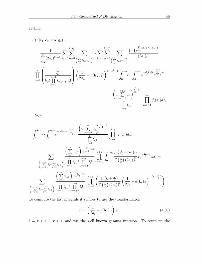
4.3. Generalized F Distribution 69
getting
F (u|c1, c2, 2m, g2) =
1r∏
v=2
(2av)bv+1
1∑
k1=0
k1b+1∑
j1=0
∑(
r∑i=1
t1,i=j1
)· · ·
1∑
kr=0
krb+r∑
jr=0
∑
(1∑
i=1tr,i=jr
)
(−1)
r∑v=1
(kv+jv−tv,1)
(2a1)j1
r∏
w=2
b+w !
bw!w−1∏v=1
tv,w+1−v!
(1
2aw
− d(kw−1)
)jv−b+v −1 ∫ +∞
0
· · ·∫ +∞
0
e−d(kr)u
r+s∑i=r+1
xi
(u
r+s∑i=r+1
xi
) r∑i=1
ti,1
r∏i=1
ti,1!
r+s∏
i=r+1
fi(xi)dxi
Now
∫ +∞
0
· · ·∫ +∞
0
e−d(kr)u
r+s∑i=r+1
xi
(u
r+s∑i=r+1
xi
) r∑i=1
ti,1
r∏i=1
ti,1!
r+s∏
i=r+1
fi(xi)dxi =
∑(
r+s∑i=r+1
li=r∑
v=1tv,1
)
(r∑
v=1
tv,1
)!u
r∑v=1
tv,1
r∏v=1
tv,1!r+s∏
v=r+1
li!
r+s∏
i=r+1
∫ +∞
0
e−(
12ai
+d(kr))xi
Γ(
gi
2
)(2ai)
gi2
xli+
gi2−1
i dxi =
∑(
r+s∑i=r+1
li=r∑
v=1tv,1
)
(r∑
v=1
tv,1
)!u
r∑v=1
tv,1
r∏v=1
tv,1!r+s∏
v=r+1
li!
r+s∏
i=r+1
(Γ(li + gi
2
)
Γ(
gi
2
)(2ai)
gi2
(1
2ai
+ d(kr)u
)−(li+gi2 )).
To compute the last integrals it suffices to use the transformation
zi =
(1
2ai
+ d(kr)u
)xi, (4.30)
i = r + 1, ..., r + s, and use the well known gamma function. To complete the

70 4. Hypothesis Testing
proof it is only needed to substitute the result just obtained in the expression of
F (u|c1, c2, 2m, g2).

5. CROSS NESTED MODELS
This chapter is started by presenting the models in this section, the balanced cross
nested random models. They are considered a special case of regular models.
5.1 Models
With Γ the set of vectors h with integer components hl = 0, ..., ul, l = 1, ...L, we
assume, for the vector y of observations, the model
y =∑
h∈Γ
X(h)β(h) + e (5.1)
where X(0) = 1n, β(0) = µ, and, with h 6= 0, X(h) =L⊗
l=1
Xl(hl) ⊗ 1r. The vectors
β(h), with h 6= 0, and e will be normal, independent, with null mean vectors and
covariance matrices σ2(h)Ic(h) and σ2In, respectively. The crossing was integrated in
the model through the use of the Kronecker matrix product, while, to have nesting,
we require that R(Xl(hl)) ⊂ R(Xl(hl + 1)), hl = 0, ..., ul−1, l = 1, ..., L. This means
that R(Xl(hl)) is strictly included in R(Xl(hl + 1)). Lastly, model orthogonality is
achieved by assuming that Ml(hl) = Xl(hl)X′l(hl) = b(hl)Ql(hl), with Ql(hl) an
orthogonal projection matrix, hl = 0, ..., ul, l = 1, ..., L. In order to have X(0) = 1n
one must have Xl(0) = 1nl, l = 1, ..., L, as well as n = rL∏
l=1
nl. Then Ql(0) =1
nl
Jnl,
l = 1, ..., L, when Jv = 1v1v ′. As we shall see, this last assumption will enable us
to derive a Jordan algebra A automatically associated to the model. Such algebra
corresponds, as it is well known, to orthogonal partitions and so, in this way, the
orthogonality of the model is ensured.

72 5. Cross Nested Models
On account of nesting we will also have the orthogonal projection matrices
Bl(0) = Ql(0) and Bl(tl) = Ql(tl) − Ql(tl − 1), tl = 1, ..., ul, l = 1, ..., L. The
Kronecker matrix product enables the construction of the orthogonal projection
matrices:
Q(h) =L⊗
l=1
Ql(hl) ⊗1
rJr, h ∈ Γ
B(t) =L⊗
l=1
Bl(tl) ⊗1
rJr, t ∈ Γ
. (5.2)
If matrices Ql(hl), hl = 0, ..., ul, have ranks rl(0) = 1 and rl(hl), hl = 1, ..., ul,
matrices Bl(tl), tl = 0, ..., ul, will have ranks gl(0) = 1 and gl(tl) = rl(tl)− rl(tl − 1),
tl = 1, ..., ul, l = 1, ..., L. Moreover, matrices Q(h) [B(t)] with u ∈ Γ [t ∈ Γ] will
have rank r(h) =L∏
l=1
rl(hl)
[g(t) =
L∏l=1
gl(tl)
].
In order to illustrate these concepts, an example: a three factor random model,
in which the second factor nests the third. We then get the model
Y =∑
h2∈Γ
X(h2)β(h2) + e, (5.3)
were h2 = (i1, i2), i = 0, 1, j = 0, 1, 2. Taking a1(1) as the number of levels of the
first factor, a2(1) the number of levels of the second and a2(2) the number of levels
of the third (nested on the second), with a1(0) = a0(2) = 1. The following matrices
are then obtained:
X(1, 0) = Ia1(1) ⊗ 1a2(1)a2(2)
X(0, 1) = 1a1(1) ⊗ Ia2(1) ⊗ 1a2(2)
X(0, 2) = 1a1(1) ⊗ Ia2(1)a2(2)
X(1, 1) = Ia1(1)a2(1) ⊗ 1a2(2)
X(1, 2) = Ia1(1)a2(1)a2(2)
, (5.4)
having also β(0, 0) = µ and β(i, j) ∼ N (0, σ2(i, j)Ic(i,j)), i = 0, 1, j = 0, 1, 2,
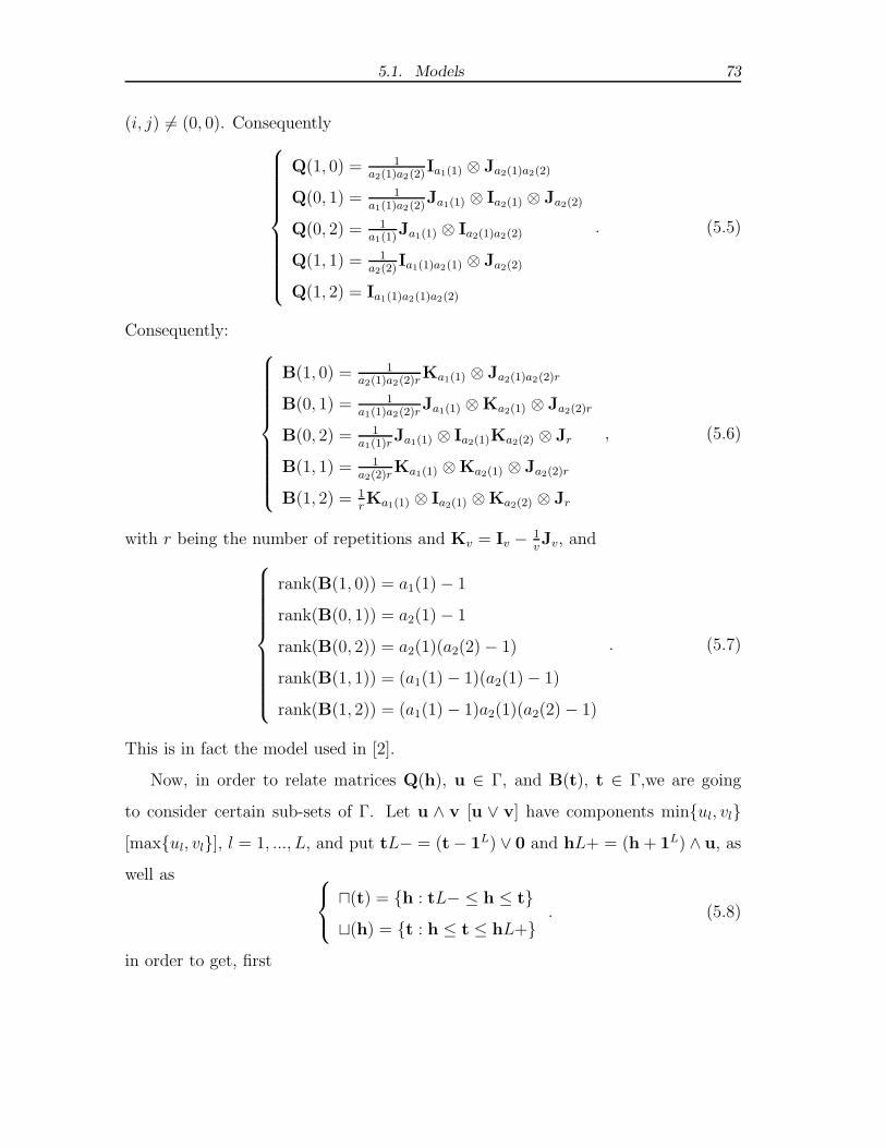
5.1. Models 73
(i, j) 6= (0, 0). Consequently
Q(1, 0) = 1a2(1)a2(2)
Ia1(1) ⊗ Ja2(1)a2(2)
Q(0, 1) = 1a1(1)a2(2)
Ja1(1) ⊗ Ia2(1) ⊗ Ja2(2)
Q(0, 2) = 1a1(1)
Ja1(1) ⊗ Ia2(1)a2(2)
Q(1, 1) = 1a2(2)
Ia1(1)a2(1) ⊗ Ja2(2)
Q(1, 2) = Ia1(1)a2(1)a2(2)
. (5.5)
Consequently:
B(1, 0) = 1a2(1)a2(2)r
Ka1(1) ⊗ Ja2(1)a2(2)r
B(0, 1) = 1a1(1)a2(2)r
Ja1(1) ⊗ Ka2(1) ⊗ Ja2(2)r
B(0, 2) = 1a1(1)r
Ja1(1) ⊗ Ia2(1)Ka2(2) ⊗ Jr
B(1, 1) = 1a2(2)r
Ka1(1) ⊗Ka2(1) ⊗ Ja2(2)r
B(1, 2) = 1rKa1(1) ⊗ Ia2(1) ⊗Ka2(2) ⊗ Jr
, (5.6)
with r being the number of repetitions and Kv = Iv − 1vJv, and
rank(B(1, 0)) = a1(1) − 1
rank(B(0, 1)) = a2(1) − 1
rank(B(0, 2)) = a2(1)(a2(2) − 1)
rank(B(1, 1)) = (a1(1) − 1)(a2(1) − 1)
rank(B(1, 2)) = (a1(1) − 1)a2(1)(a2(2) − 1)
. (5.7)
This is in fact the model used in [2].
Now, in order to relate matrices Q(h), u ∈ Γ, and B(t), t ∈ Γ,we are going
to consider certain sub-sets of Γ. Let u ∧ v [u ∨ v] have components minul, vl[maxul, vl], l = 1, ..., L, and put tL− = (t− 1L) ∨ 0 and hL+ = (h + 1L) ∧ u, as
well as
⊓(t) = h : tL− ≤ h ≤ t⊔(h) = t : h ≤ t ≤ hL+
. (5.8)
in order to get, first

74 5. Cross Nested Models
Proposition 2. Q(h) =∑t≤h
B(t), as well as
B(t) =∑
h∈⊓(t)
(−1)m(h,t)Q(h)
with m(h, t) the number of components of h that are smaller than the corresponding
components of t.
Proof. The first part of the thesis follows from Ql(hl) =∑
tl≤hl
Bl(tl), hl = 0, ..., ul,
l = 1, ..., L, and from the distributive properties of the Kronecker product. Nextly,
the first part of the thesis enables the writing of
∑
h∈⊓(t)
(−1)m(h,t)Q(h) =∑
h∈⊓(t)
(−1)m(h,t)∑
v≤h
B(v).
If v < t, B(v) will enter in the terms of the h such that v ≤ h ≤ t. Since it is
possible to choose in(m(v,t)
a
)ways a of the components of h that are smaller than
the corresponding components of t, this being the number of vectors h such that
m(h, t) = a. If m(v, t) > 0 the coefficient of B(v) in the previous expression of∑
h∈⊓(t)
(−1)m(h,t)Q(h) will be
m(v,t)∑
a=0
(m(v, t)
a
)(−1)a = 0
since a = m(h, t). If m(h, t) = 0, v = h = t and B(v) only enters, with coefficient
one, in∑
h∈⊓(t)
(−1)m(h,t)∑v≤h
B(v). Thus
B(t) =∑
v∈⊓(t)
(−1)m(v,t)Q(v).
Corollary 3. With S(t) = ‖B(t)y‖2,
S(t) =∑
h∈⊓(t)
(−1)m(h,t)‖Q(h)y‖2 =∑
h∈⊓(t)
(−1)m(h,t)
b(h)‖X′(h)y‖2

5.1. Models 75
with b(h) = rL∏
l=1
bl(hl).
Proof. The first part of the thesis follows directly from Proposition 2. As to the
second part, since X(h)X′(h) = b(h)Q(h) and orthogonal projection matrices are
idempotent and symmetric,
‖Q(h)y‖2 = y′Q′(h)Q(h)y = y′Q(h)y
= y′
(1
b(h)X(h)X′(h)
)y =
1
b(h)‖X′(h)y‖2,
the rest of the proof being straightforward.
Besides matrices B(t), t ∈ Γ, take
B = In − B(u) = In −∑
t∈Γ
B(t) (5.9)
to obtain a basis for a Jordan algebra A. This basis is the sole basis of A constituted
by mutually orthogonal orthogonal projection matrices. This will be the principal
basis of A. Moreover matrices Q(h), h ∈ Γ, and In belong to A. R(B(t)), with
t ∈ Γ, and R(B) constitute an orthogonal partition of Rn into mutually orthogonal
sub-spaces.
The mean vector and covariance matrix of y will be, with σ2(0) = 0
E[y] = 1nµ
V[y] =∑h∈Γ
σ2(h)M(h) + σ2In =∑t∈Γ
γ(t)B(t) + σ2B(5.10)
with
γ(t) = σ2 +∑
h≥t
b(h)σ2(h), (5.11)
since σ2(h)M(h) = b(h)σ2(h)∑t≤h
B(t), h ∈ Γ. It is the fact that V[y] is a linear
combination of the matrices in the basis of A, which are mutually orthogonal, that
gives the model it’s orthogonality.

76 5. Cross Nested Models
Still using model (5.3), it is easy to check that
γ(1, 0) = a2(1)a2(2)rσ2(1, 0) + a2(2)rσ2(1, 1) + rσ2(1, 2) + σ2
γ(0, 1) = a1(1)a2(2)rσ2(0, 1) + a1(1)a2(1)rσ2(0, 2) + a2(2)rσ2(1, 1)
+ rσ2(1, 2) + σ2
γ(0, 2) = a1(1)a2(1)rσ2(0, 2) + a2(2)rσ2(1, 1) + rσ2(1, 2) + σ2
γ(1, 1) = a2(2)rσ2(1, 1) + rσ2(1, 2) + σ2
γ(1, 2) = rσ2(1, 2) + σ2
. (5.12)
Going over to the balanced case in which will be L groups of u1, ..., uL factors,
i.e., the generalization of model (5.3). When ul > 1 there is balanced nesting for
the factors of the l-th group. This is, for each of the al(1) levels of the first factor
in the group there will be al(2) levels of the second factor. Then, for each of the
al(1)× al(2) levels of the second factor there will be al(3) of the third factor, and so
on.
Xl(hl) = Icl(hl) ⊗ 1bl(hl), hl = 0, ..., ul, l = 1, ..., L (5.13)
with cl(hl) =hl∏
t=1
al(t) and bl = cl(ul)/cl(hl), as well as
Ml(hl) = Icl(hl) ⊗(
1
bl(hl)Jbl(hl)
)=
1
bl(hl)Ql(hl),
hl = 0, ..., ul, l = 1, ..., L (5.14)
where Ql(hl) = Icl(hl) ⊗(
1
bl(hl)Jbl(hl)
), hl = 0, ..., ul, l = 1, ..., L. Defining Kv =
Iv −1
vJv we also get
Bl(tl) = Icl(tl−1) ⊗ Kal(tl) ⊗(
1
bl(tl)Jbl(tl)
)= A′
l(tl)Al(tl),
tl = 1, ..., ul, l = 1, ..., L (5.15)

5.2. Estimators 77
with
Al(tl) =1√bl(tl)
Icl(tl−1) ⊗ Kal(tl) ⊗ 1bl(tl)′, tl = 1, ..., ul, l = 1, ..., L.
Putting Al(0) = 1nl ′, l = 1, ..., L, and, if there are r replicates for each factor
combination, define the following matrices
A(t) =1√r
L⊗
l=1
Al(tl) ⊗ 1r ′, t ∈ Γ.
The sums of squares and corresponding degrees of freedom for a given factor or
interaction will be
S(t) = ‖A(t)y‖2 , t ∈ Γ
g(t) =L∏
l=1
gl(tl) =L∏
l=1
(cl(tl) − cl(tl − 1)) , t ∈ Γ(5.16)
with cl(−1) = 0 for l = 1, ..., L.
Just for the record, consider another special case. Let Pl be a nl ×nl orthogonal
projection matrix whose first column vector is1√nl
1nl, l = 1, .., L. With cl(0) = 1
and cl(hl) < cl(hl + 1) ≤ nl, hl = 1, ..., ul − 1, take Xl(hl) to be constituted by the
first cl(hl) columns of Pl, l = 1, ..., L. It is easy to see that the assumptions hold in
this case which is distinct from the balanced one. Putting A(0) = X′l(0), l = 1, ..., L
Xl(tl) =[
Xl(tl − 1) A′l(tl)
]tl = 1, ..., ul, l = 1, ..., L (5.17)
and A(t) =L⊗
l=1
Al(tl) ⊗ 1r ′ expressions in (5.16) continue to hold.
5.2 Estimators
Note that for the models considered, the minimal complete statistics will be: y• =1
n1n′y, S(t), with t ∈ Γ, and S = ‖By‖2. The statistics S(t), with t ∈ Γ, are given
by the first expression in (5.16).

78 5. Cross Nested Models
When 0 < t ≤ u, B(t)y will be normal with null mean vector and covariance
matrix γ(t)B(t), so that S(t) will be the product by γ(t) of a central chi-square
with g(t) = rank(B(t)) degrees of freedom, denoted by S(t) ∼ γ(t)χ2(g(t)). Likewise
S ∼ σ2χ2(g), with g = n− r(u). Moreover,
F(t1, t2) =g(t2)
g(t1)· S(t1)
S(t2)(5.18)
will be the product byγ(t1)
γ(t2)of a random variable with central F distribution with
g(t1) and g(t2) degrees of freedom. Whenever g(t2) > 2, E[F(t1, t2)] =g(t2)
g(t2) − 2·
γ(t1)
γ(t2)and so we have the UMVUE
(γ(t1)
γ(t2)
)=g(t2) − 2
g(t2)· S(t1)
S(t2). (5.19)
Later on these estimators will be used. If fq:r,s is the quantile, for probability q, of
the central F distribution with r and s degrees of freedom we have, forγ(t1)
γ(t2), the
(1 − q) × 100% confidence interval
[F(t1, t2)
f1− q
2:g1,g2
,F(t1, t2)
f q
2:g1,g2
]
with gi = g(ti), i = 1, 2.
The 1 − q level upper bound will likewise beF(t1, t2)
f1−q:g1,g2
The sets ⊓(t) and ⊔(t) were defined in the preceding section and established
Proposition 2.
Proposition 3. Whenever m(h) = m(h,u) > 0,
σ2(h) =1
b(h)
∑
t∈⊔(h)
(−1)m(h,t)γ(t).
Proof. From the definition of γ(t),
∑
t∈⊔(h)
(−1)m(h,t)γ(t) =∑
t∈⊔(h)
(−1)m(h,t)
(
σ2 +∑
v≥t
b(v)σ2(v)
)
.

5.2. Estimators 79
Now, in ⊔(h) we have(m(h)
z
)(with z ranging from 0 to m(h)) vectors t such that
m(h, t) = z, since this is the number of choices of z components of h, from the
m(h) components that are smaller than those of u. So, these components of h can
be increased by 1, the resulting vector still belonging to ⊔(h). Thus, the coefficient
of σ2 will bem(h)∑z=0
(m(h)
z
)(−1)z = 0. Likewise, if v > h, σ2(v) appears in the terms
associated with the t ∈ ⊔(h) such that t ≤ v. It is possible to reason as before
to show that there are(m(h,v)
z
), z = 0, ...,m(h,v), such vectors t ∈ ⊔(h) with
m(h,v) = z, and so, the coefficient of b(h)σ2(h) will bem(h,v)∑
z=0
(m(h,v)
z
)(−1)z = 0.
Lastly when v = h, b(v)σ2(v) = b(h)σ2(h) only enters in the term associated with
t = h with coefficient 1, so that∑
t∈⊔(h)
(−1)m(h,t)γ(t) = b(h)σ2(h) and the thesis is
established.
Corollary 4. γ(t) =S(t)
g(t), t ∈ Γ and, if m(h) > 0,
σ2(h) =1
b(h)
∑
t∈⊔(h)
(−1)m(h,t)γ(t)
will be UMVUE.
Moreover, for σ2 and σ2(u) there are the UMVUE
σ2 =S
g
σ2(u) =1
b(u)(γ(u) − σ2),
(5.20)
since S ∼ σ2χ2(g) and γ(u) = σ2 + b(u)σ2(u). Note that m(h) = 0 if and only if
h = u.
Let ⊔(h)+ and ⊔(h)− be the vectors of ⊔(h) for which m(h, t) is even or is odd.
If m(h) > 0, with σ2(h)+ =1
b(h)
∑t∈⊔(h)+
γ(t) and σ2(h)− =1
b(h)
∑t∈⊔(h)−
γ(t) we
have
σ2(h) = σ2(h)+ − σ2(h)−. (5.21)

80 5. Cross Nested Models
We will also have the UMVUE estimators
σ2(h)+ =1
b(h)
∑t∈⊔(h)+
γ(t)
σ2(h)− =1
b(h)
∑t∈⊔(h)−
γ(t).(5.22)
Besides through completeness of the statistics, it will now be shown through an
alternative method that the estimators obtained are efficient in the Fisher sense.
It is proved in [3] that
det (V[y]) =
(∏
t∈Γ
γ(t)g(t)
)(σ2)
g, (5.23)
so that, if η has components µ, γ(t), 0 < t ≤ u, and σ2 one gets the log-likelihood
l(η) = − n
2γ(0)(y• − µ)2 − 1
2
∑
0≤t≤u
S(t)
γ(t)− S
2σ2− n
log(2π)
− 1
2
∑
t∈Γ
g(t) logγ(t) − g
2log σ2. (5.24)
γ(0) was omitted from the components of η since this parameter is clearly a function
of the γ(t), 0 < t ≤ u. It is now straightforward to show that µ = y•, γ(t), 0 <
t ≤ u, and σ2 are maximum likelihood estimators and that their Fisher information
matrix
Z(η) = E[grad(l(η)) (grad(l(η)))′
](5.25)
is the diagonal matrix with principal elementsn
2γ(0),
n
2γ(0),g(t)
2γ(t), 0 < t ≤ u, and
g
2σ2. Since these are the inverses of the variances of these estimators we see that
the Cramer-Rao lower bound for the variance of unbiased estimators is attained for
these estimators,
V[η]−1 = Z(η). (5.26)
Let θ have components µ, σ2(t), 0 < t ≤ u, and σ2. Then θ = Kη with K a regular
matrix so that η = K−1θ and, using the new parameters, we have for the gradient
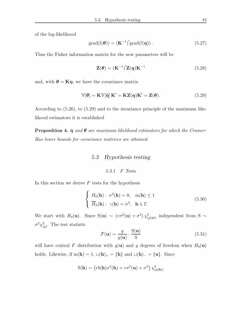
5.3. Hypothesis testing 81
of the log-likelihood
grad(l(θ)) = (K−1)′grad(l(η)) . (5.27)
Thus the Fisher information matrix for the new parameters will be
Z(θ) = (K−1)′Z(η)K−1 (5.28)
and, with θ = Kη, we have the covariance matrix
V[θ] = KV[η]K′ = KZ(η)K′ = Z(θ). (5.29)
According to (5.26), to (5.29) and to the invariance principle of the maximum like-
lihood estimators it is established
Proposition 4. η and θ are maximum likelihood estimators for which the Cramer-
Rao lower bounds for covariance matrices are attained.
5.3 Hypothesis testing
5.3.1 F Tests
In this section we derive F tests for the hypothesis
H0(h) : σ2(h) = 0, m(h) ≤ 1
H0(h) : γ(h) = σ2, h ∈ Γ.(5.30)
We start with H0(u). Since S(u) ∼ (rσ2(u) + σ2)χ2(g(u)) independent from S ∼
σ2χ2(g). The test statistic
F(u) =g
g(u)· S(u)
S(5.31)
will have central F distribution with g(u) and g degrees of freedom when H0(u)
holds. Likewise, if m(h) = 1, ⊔(h)+ = h and ⊔(h)− = u. Since
S(h) ∼(rb(h)σ2(h) + rσ2(u) + σ2
)χ2
(g(h))
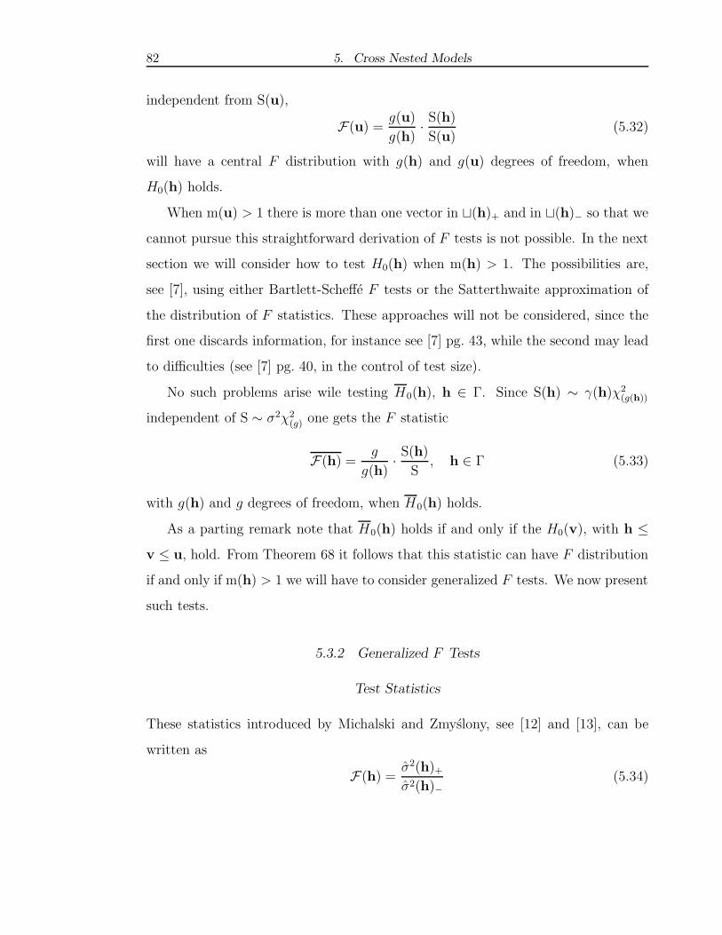
82 5. Cross Nested Models
independent from S(u),
F(u) =g(u)
g(h)· S(h)
S(u)(5.32)
will have a central F distribution with g(h) and g(u) degrees of freedom, when
H0(h) holds.
When m(u) > 1 there is more than one vector in ⊔(h)+ and in ⊔(h)− so that we
cannot pursue this straightforward derivation of F tests is not possible. In the next
section we will consider how to test H0(h) when m(h) > 1. The possibilities are,
see [7], using either Bartlett-Scheffe F tests or the Satterthwaite approximation of
the distribution of F statistics. These approaches will not be considered, since the
first one discards information, for instance see [7] pg. 43, while the second may lead
to difficulties (see [7] pg. 40, in the control of test size).
No such problems arise wile testing H0(h), h ∈ Γ. Since S(h) ∼ γ(h)χ2(g(h))
independent of S ∼ σ2χ2(g) one gets the F statistic
F(h) =g
g(h)· S(h)
S, h ∈ Γ (5.33)
with g(h) and g degrees of freedom, when H0(h) holds.
As a parting remark note that H0(h) holds if and only if the H0(v), with h ≤v ≤ u, hold. From Theorem 68 it follows that this statistic can have F distribution
if and only if m(h) > 1 we will have to consider generalized F tests. We now present
such tests.
5.3.2 Generalized F Tests
Test Statistics
These statistics introduced by Michalski and Zmyslony, see [12] and [13], can be
written as
F(h) =σ2(h)+
σ2(h)−(5.34)
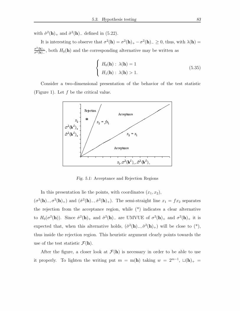
5.3. Hypothesis testing 83
with σ2(h)+ and σ2(h)− defined in (5.22).
It is interesting to observe that σ2(h) = σ2(h)+ −σ2(h)− ≥ 0, thus, with λ(h) =
σ2(h)+σ2(h)−
, both H0(h) and the corresponding alternative may be written as
H0(h) : λ(h) = 1
H1(h) : λ(h) > 1.(5.35)
Consider a two-dimensional presentation of the behavior of the test statistic
(Figure 1). Let f be the critical value.
Fig. 5.1: Acceptance and Rejection Regions
In this presentation lie the points, with coordinates (x1, x2),
(σ2(h)−, σ2(h)+) and (σ2(h)−, σ
2(h)+). The semi-straight line x1 = fx2 separates
the rejection from the acceptance region, while (*) indicates a clear alternative
to H0(σ2(h)). Since σ2(h)+ and σ2(h)− are UMVUE of σ2(h)+ and σ2(h)+ it is
expected that, when this alternative holds, (σ2(h)−, σ2(h)+) will be close to (*),
thus inside the rejection region. This heuristic argument clearly points towards the
use of the test statistic F(h).
After the figure, a closer look at F(h) is necessary in order to be able to use
it properly. To lighten the writing put m = m(h) taking w = 2m−1, ⊔(h)+ =

84 5. Cross Nested Models
t1, ..., tw and ⊔(h)− = tw+1, ..., t2w. Let g1 and g2 have components g1,j = g(tj)
and g2,j = g(tj+w), j = 1, ..., w, where we can assume that gi,1 = mingi,1, ..., gi,wand gi,w = maxgi,1, ..., gi,w, i = 1, 2. Then
F(h) = λ(h)
w∑j=1
p1,j
g1,j
χ2(g1,j)
w∑j=1
p2,j
g2,j
χ2(g2,j)
, (5.36)
with p1,j =γ(tj)
σ2(h)+and p2,j =
γ(tj+w)
σ2(h)−, j = 1, ..., w, and, as before, λ(h) =
σ2(h)+
σ2(h)−.
Sincew∑
j=1
p1,j =w∑
j=1
p2,j = 1, F(h) will be the product by λ(h) of the quotient of two
convex combinations of independent central chi-squares divided by their degrees of
freedom. Thus, it is natural to consider F(h) as a generalized F statistic. The p1,j
and p2,j , j = 1, ..., w will be the components of vectors p1 and p2. These vectors
will be nuisance parameters. Since
p1,j =
γ(tj)
γ(tw)w∑
j′=1
γ(tj′ )
γ(tw)
, j = 1, ..., w
p2,j =
γ(tj+w)
γ(t2w)w∑
j′=1
γ(tj′+w)
γ(t2w)
, j = 1, ..., w,
(5.37)
( γ(tj)
γ(tw)
)and
(γ(tj+w)
γ(t2w)
)can be used to estimate p1,j and p2,j , j = 1, ..., w. Now,
when H0(h) holds,
F(h) =Y1
Y2, (5.38)
with Y1 =w∑
j=1
pi,j
χ2(gi,j)
gi,j
, i = 1, 2. Since the Y1 and Y2 are independent with mean
value 1, and the partial derivatives ofY1
Y2
, at point (1, 1), are 1 and −1, one gets,
when H0(h) holds
F(h) ≈ 1 + (Y1 − 1) − (Y2 − 1), (5.39)

5.3. Hypothesis testing 85
so that, according to the independence of Y1 and Y2
E[F(h)] ≈ 1
V[F(h)] ≈ V[Y1] + V[Y2]. (5.40)
Also
V[Yi] = 2w∑
j=1
p2i,j
gi,j
, i = 1, 2. (5.41)
Looking at the Figure 2 one is led to think that, when H0(h) holds, the probability
Fig. 5.2: Critical Value
of rejection increases with2∑
i=1
V[Yi]. Putting gi =w∑
j=1
gi,j and ui,j = pi,j −1
gi
gi,j,
j = 1, ..., w, i = 1, 2,
V[Yi] =2
gi
+ 2w∑
j=1
u2i,j
gi,j
, i = 1, 2 (5.42)
so that, according to (5.41) and (5.42),2
gi
< V[Yi] <2
gi,1, i = 1, 2. It is interesting
to observe that when V[Yi] attains it´s lower bound, Yi is a central chi-square with gi
degrees of freedom divided by this number and when V[Yi] attains it´s upper bound,
Yi is a central chi-square with gi,1 degrees of freedom divided by the same number.
Thus, when both lower or both upper bounds are attained, F(h) has, when H0(h)
holds, the central F distribution with g1 and g2 or g1,1 and g2,1 degrees of freedom.

86 5. Cross Nested Models
In the balanced case there are some restrictions on the pi,j , j = 1, ..., w, i = 1, 2.
WhenH0(h) holds σ2(h)+ = σ2(h)−, and so γ(h) = γ(t1) = maxγ(t1), ..., γ(tw) ≥maxγ(tw+1), ..., γ(t2w), so that
p1,1 = maxp1,1, ..., p1,w ≥ 1
w>g(h)
g1
p1,1 ≥ maxp2,1, ..., p2,w. (5.43)
When w = 2 one can take p1,1 = p1, p1,2 = 1 − p1, p2,1 = p2 and p2,2 = 1 − p2 to
get
maxp2, 1 − p2 ≤ p1. (5.44)
Getting back to the general case in order to control the first type error, one can
• place under the least favorable situation in which, as we saw, we have an F
test with g1,1 and g2,1 degrees of freedom;
• use more completely the set of complete sufficient statistics. One then obtains,
besides the test statistic, estimates to the nuisance parameters. In this case
one will be carrying out an adaptative procedure similar to the one carried
out in [1] and [35]. Likewise one may think we are using ancillary statistics,
see [26].
Restricting to the balanced case, the goal is to see when one or both of the
evenness conditions hold. Since
g(h) =L∏
l=1
gl(hl) (5.45)
it suffices that one of the gl(hl), l = 1, ..., L, is even for g(h) to be even. Besides
this, with 0 ≤ hl ≤ ul,
gl(0) = 1, l = 1, ..., L
gl(hl) =
(hl−1∏tl=1
al(tl)
)(al(hl) − 1) , hl = 1, ..., ul, l = 1, ..., L,
(5.46)

5.3. Hypothesis testing 87
were al(hl) is the number of factors of the hl-th factor in the l-th group of nested
factors, and0∏
t=1
al(t) = 1, l = 1, , ..., L. Thus if gl(hl), with l ≥ 1, is odd, al(hl) must
be even as well as gl(h∗) with hl ≤ h∗ ≤ ul. Thus in the sequence gl(1), ..., gl(ul)
there can be only one odd number. This observation clearly points towards evenness
conditions holding quite often.Consider the sets of indexes C(h) = j : hj < uj and
D(h) = l : hl > 0, putting u(h) = #(C(h)) and o(h) = #(D(h)) − 1. With ql(hl)
the number of even numbers in the pair (gl(hl), gl(hl + 1)), one get ql(0) ≤ 1 since
gl(0) = 1 so that only gl(1) may be even. Put also
k(h) = maxl∈C(h)
ql(hl)
t(h) = minl∈C(h)
ql(hl).(5.47)
Establish
Proposition 5. If k(h) = 2 or if there exists l′ /∈ C(h) such that gl′(ul′) is even
both evenness conditions are satisfied.
Proof. If k(h) = 2 there will be l ∈ C(h) such that gl(hl) and gl(hl + 1) are even.
Since either of these will be a factor in g(h∗) whatever h∗ ∈ ⊔(h), the first part of
the thesis is established. The second part follows from gl′(ul′) being, if it exists, a
factor from whatever g(h∗) with h∗ ∈ ⊔(h).
Nextly one gets
Proposition 6. If k(h) = t(h) = 1 one of the two evenness conditions holds.
Proof. If k(h) = t(h) = 1, whenever l ∈ C(h), gl(hl)) or gl(hl + 1) is even but not
both since k(h) = 1. For g(hL∗), with hL∗ ∈ ⊔(h), to be odd one must have, for
l ∈ C(h), h∗l = hl when gl(hl) is odd or hl + 1 when gl(hl) is even. Thus there is at
most one vector h0 ∈ ⊔(h) such that g(h0) is odd.
Then, if h0 ∈ ⊔(h)+ the first evenness condition holds and if ⊔(h)− the second
evenness condition holds.

88 5. Cross Nested Models
Corollary 5. If o(h) = L− 1 at least one of the evenness conditions holds.
Proof. If o(h) = L−1 we have hl ≥ 1, l = 1, ..., L and so ql(hl) ≥ 1, for all l ∈ C(h),
since, when gl(hl) is odd gl(hl +1) is even, thus t(h) ≥ 1 and the thesis follows from
Propositions 5 and 6.
Corollary 6. If al,1 is odd, l = 1, ..., L, at least one of the evenness conditions holds
for all h ∈ Γ.
Proof. ql(0) = 1, l = 1, ..., L, as well as ql(hl) ≥ 1, hl = 1, ..., ul−1. Thus t(h) ≥ 1
for all h ∈ Γ. To complete the proof, apply Propositions 5 and 6.
These results show that quite often one can get exact expressions for F (z|c1, c2, g1, g2).
This is interesting in itself and enables accuracy checking applying Monte-Carlo
methods to evaluate F (z|c1, c2, g1, g2) (see [1]).
6. FINAL REMARKS
Although some proposals were made regarding pendent issues on linear models,
specially in model structure, estimation of fixed effects and variance components
and hypothesis testing, a lot of questions remain unanswered.
• When BLUE are not obtainable, what to do? How to derive explicit formulas
for LBLUE (locally best unbiased estimators)? An analogous problem (but
somewhat more complex) arises with variance components.
• What approach to take with general unbalanced data? The results obtained
work under the assumption of model orthogonality, but a systematic approach
for unbalanced models is needed. A possible solution is the use of U statistics
in the estimation of parameters.
• Normality. At what extend is it necessary? And can it be attained asymptot-
ically for general linear models and if so, in what conditions?
• It is logical to think of the generalization of model algebraic structure and the
generalized F test to the multivariate case. It is a pendent subject.
These are merely some suggestions for future research. It is a truism that the
more answers are obtained the more questions arise.

90 6. Final Remarks

BIBLIOGRAPHY
[1] Miguel Fonseca, Joao Tiago Mexia, and Roman Zmyslony. Exact distribution
for the generalized F tests. Discuss. Math., Probab. Stat., 22(1-2):37–51, 2002.
[2] Miguel Fonseca, Joao Tiago Mexia, and Roman Zmyslony. Estimating and
Testing of Variance Components: an Application to a Grapevine Experiment.
Biometrical Letters, 40:1–7, 2003.
[3] Miguel Fonseca, Joao Tiago Mexia, and Roman Zmyslony. Estimators and tests
for variance components in cross nested orthogonal designs. Discuss. Math.,
Probab. Stat., 23(2):175–201, 2003.
[4] Miguel Fonseca, Joao Tiago Mexia, and Roman Zmyslony. Binary opera-
tions on Jordan algebras and orthogonal normal models. Linear Algebra Appl.,
417(1):75–86, 2006.
[5] S. Gnot, W. Klonecki, and R. Zmyslony. Best unbiased linear estimation, a
coordinate free approach. Probab. Math. Stat., 1:1–13, 1980.
[6] P. Jordan, J. von Neumann, and Eugene P. Wigner. On an algebraic general-
ization of the quantum mechanical formalism. 1934.
[7] Andre I. Khuri, Thomas Mathew, and Bimal K. Sinha. Statistical tests for
mixed linear models. Wiley Series in Probability and Mathematical Statistics,
Applied Section. New York, NY: Wiley., 1998.
92 Bibliography
[8] Lynn Roy LaMotte. A canonical form for the general linear model. Ann. Stat.,
5:787–789, 1977.
[9] E.L. Lehmann. Testing statistical hypotheses. Reprint of the 2nd ed. publ. by
Wiley 1986. New York, NY: Springer. , 1997.
[10] E.L. Lehmann and George Casella. Theory of point estimation. 2nd ed. Springer
Texts in Statistics. New York, NY: Springer. , 1998.
[11] James D. Malley. Statistical applications of Jordan algebras. Lecture Notes in
Statistics (Springer). 91. New York, NY: Springer- Verlag. , 1994.
[12] Andrzej Michalski and Roman Zmyslony. Testing hypotheses for variance com-
ponents in mixed linear models. Statistics, 27(3-4):297–310, 1996.
[13] Andrzej Michalski and Roman Zmyslony. Testing hypotheses for linear func-
tions of parameters in mixed linear models. Tatra Mt. Math. Publ., 17:103–110,
1999.
[14] Alexander M. Mood, Franklin A. Graybill, and Duane C. Boes. Introduction to
the theory of statistics. 3rd ed. McGraw-Hill Series in Probability and Statistics.
New York etc.: McGraw- Hill Book Company. , 1974.
[15] C.Radhakrishna Rao and M.Bhaskara Rao. Matrix algebra and its applications
to statistics and econometrics. Singapore: World Scientific Publishing. , 1998.
[16] Henry Scheffe. The analysis of variance. Repr. of the 1959 orig. Wiley Classics
Library. New York, NY: Wiley. , 1999.
[17] Mark J. Schervish. Theory of statistics. Springer Series in Statistics. New York,
NY: Springer-Verlag., 1995.

Bibliography 93
[18] James R. Schott. Matrix analysis for statistics. Wiley Series in Probability and
Mathematical Statistics. New York, NY: Wiley. , 1997.
[19] Shayle R. Searle, George Casella, and Charles E. McCulloch. Variance com-
ponents. Wiley Series in Probability and Statistics. Hoboken, NJ: John Wiley
& Sons., 2006.
[20] J. Seely. Linear spaces and unbiased estimation. Ann. Math. Stat., (41):1725—
1734, 1970.
[21] J. Seely. Linear spaces and unbiased estimation. an aplication to the mixed
linear model. Ann. Math. Stat., (41):1735—1748, 1970.
[22] J. Seely. Quadratic subspaces and completeness. Ann. Math. Stat., (42):710—
721, 1971.
[23] J. Seely and G. Zyskind. Linear spaces and minimum variance unbiased esti-
mation. Ann. Math. Stat., (42):691—703, 1971.
[24] Justus Seely. Completeness for a family of multivariate normal distributions.
Ann. Math. Stat., 43:1644–1647, 1972.
[25] Justus Seely. Minimal sufficient statistics and completeness for multivariate
normal families. Sankhya, Ser. A, 39:170–185, 1977.
[26] Thomas A. Severini. Likelihood methods in statistics. Oxford Statistical Science
Series. 22. Oxford: Oxford University Press. , 2000.
[27] S.D. Silvey. Statistical inference. Reprinted with corrections. Monographs on
Applied Probability and Statistics. London: Chapman and Hall Ltd. 192 p.
£2.30 , 1975.

94 Bibliography
[28] Samaradasa Weerahandi. Generalized confidence intervals. J. Am. Stat. Assoc.,
88(423):899–905, 1993.
[29] Samaradasa Weerahandi. Exact statistical methods for data analysis. 2nd print.
Berlin: Springer-Verlag., 1996.
[30] David Williams. Probability with martingales. Cambridge etc.: Cambridge
University Press. , 1991.
[31] Leping Zhou and Thomas Mathew. Some tests for variance components using
generalized p values. Technometrics, 36(4):394–402, 1994.
[32] R. Zmyslony. On estimation of parameters in linear models. Zastosow. Mat.,
15:271–276, 1976.
[33] Roman Zmyslony. A characterization of best linear unbiased estimators in the
general linear model. 1980.
[34] Roman Zmyslony. Completeness for a family of normal distributions. Mathe-
matical statistics, Banach Cent. Publ. 6, 355-357 (1980)., 1980.
[35] Stefan Zontek. Robust estimation in linear model for spatially located sensors
and random input. Tatra Mt. Math. Publ., 17:301–310, 1999.