Embed Size (px)
Citation preview

1
Achieving Energy Efficiency and Reliability forData Dissemination in Duty-Cycled WSNs
Kai Han, Jun Luo, Liu Xiang, Mingjun Xiao and Liusheng Huang
Abstract—Because data dissemination is crucial to WirelessSensor Networks (WSNs), its energy-efficiency and reliabilityare of paramount importance. While achieving these two goalstogether is highly non-trivial, the situation is exacerbated if WSNnodes are duty-cycled (DC) and their transmission power isadjustable. In this paper, we study the problem of minimizing theexpected total transmission power for reliable data dissemination(multicast/broadcast) in DC-WSNs. Due to the NP-hardness ofthe problem, we design efficient approximation algorithms withprovable performance bounds for it. To facilitate our algorithmdesign, we propose the novel concept of Time-Reliability-Power(TRP) space as a general data structure for designing datadissemination algorithms in WSNs, and the performance ratiosof our algorithms based on the TRP space are proven to beO(log ∆ log k) for both multicast and broadcast, where ∆ is themaximum node degree in the network and k is the number ofsource/destination nodes involved in a data dissemination session.We also conduct extensive simulations to firmly demonstrate theefficiency of our algorithms.
I. INTRODUCTION
Designing effective data dissemination mechanisms forWireless Sensor Networks (WSNs) is of paramount impor-tance, as WSNs rely on data dissemination to carry criticalcommands or code updates from a sink to a set of (or all) nodesin the networks [1], [2]. Reliability and energy-efficiency areperhaps the most crucial requirements for data disseminationdue to the notorious packet-losses in wireless communicationsand the limited power supply of sensor nodes.
Achieving reliability and energy-efficiency simultaneouslyis by no means trivial, and the problem gets even more chal-lenging when modern WSNs’ features such as duty-cyclingand power-adjustability are taken into account. On one hand,in a Duty-Cycled WSN (DC-WSN), nodes usually switch be-tween active/dormant states periodically, which imposes extradifficulty on attaining energy-efficiency even without regardingreliability [3]–[5]. On the other hand, nodes’ capability ofadjusting the transmission power (tx-power) to several levels
This work was supported in part by the AcRF Tier 2 Grant ARC15/11and the National Natural Science Foundation of China (No. 61103007). Apreliminary version of this paper appeared in ACM MobiHoc 2013, Bangalore,India, July 29–August 1, 2013.
Kai Han is with School of Computer Engineering, Nanyang TechnologicalUniversity, Singapore, and also with School of Computer Science, ZhongyuanUniversity of Technology, China. E-mail: [email protected].
Jun Luo is with School of Computer Engineering, Nanyang TechnologicalUniversity, Singapore. E-mail: [email protected].
Liu Xiang is with Institute for Infocomm Research (I2R), A*STAR,Singapore. This work was done when she was working as a PhD candidatein NTU. E-mail: [email protected].
Mingjun Xiao and Liusheng Huang are with School of Computer Scienceand Technology, University of Science and Technology of China, China. E-mail: {xiaomj, lshuang}@ustc.edu.cn.
brings out a tradeoff between reliability and energy-efficiency,as a node can increase its tx-power to improve link reliabilityat the cost of higher energy consumption [6]. All theseentangled features make it extremely challenging to designenergy-efficient reliable data dissemination mechanisms forDC-WSNs.
Despite major efforts on energy-efficient data disseminationin wireless networks, a large body of them have taken the over-optimistic assumption of error-free wireless transmissions [3],[4], [7]–[10]. Other proposals considering unreliable linksroughly follow two lines. One line bears the common objectiveof minimizing the expected tx-power consumption under guar-anteed reliability, but they are designed only for Always-ActiveWireless Networks (AAWNs) [6], [11], [12]. This batch ofwork has unanimously concentrated on unicasting or employ-ing unicasting to achieve multicasting [6] without leveragingthe Wireless Broadcast Advantage (WBA). Another line aimsat reducing the tx-power consumption for broadcasting in DC-WSNs without a stringent requirement on reliability. As arepresentative proposal in this line, [13] proposed a tree-basedopportunistic flooding approach. However, the broadcast treeused in [13] is constructed for very low duty-cycle, hencetransmissions are still done through unicasting (similar to [6]).
In this paper, we present the first study on energy-efficientreliable data dissemination in DC-WSNs with guaranteedperformance. We aim to minimize the expected total tx-powerconsumption in multicasting or broadcasting under guaranteedreliability, and we take into account WBA, unreliable links,power-adjustability and duty-cycling holistically. Given thatthe resulting Energy efficient Reliable Data Dissemination(ERDD) problem is NP-hard, we propose approximation algo-rithms for it with performance ratios of O(ln ∆ ln k), where ∆is the maximum node degree in the network and k is the totalnumber of nodes involved in a multicast/broadcast session.We also show the efficiency of our approach by extensivesimulation results.
The rest of our paper is organized as follows. Section IIreviews related work. Section III provides our models andproblem definitions. In Section IV, we present our approxi-mation algorithms. The performance ratios of our algorithmsare analyzed in Section V. Section VI reports our simulationresults and Section VII concludes the paper. To maintainfluency, all the proof sketches of our lemmas/theorems arepostponed to the Appendix.
II. RELATED WORK
Always-Active Wireless Networks with Reliable Links: Min-energy multicast/broadcast and related topology control prob-
2
lems in AAWNs with reliable links have been studied exten-sively in the literature. As these problems are generally NP-hard [14], many approximation algorithms have been proposedunder different network models and constraints. The seminalwork in [15] provides upper and lower bounds for the powerassignment problem under different connectivity constraints,and proposes asymptotically optimal O(log n) approximationalgorithms for min-power (strong or symmetric) connectivityand min-power broadcasting problems. The work in [16] pro-poses an approximation algorithm for the min-power broadcastrouting problem in wireless ad hoc networks that achievesan exponentially better approximation ratio compared to theMinimum Spanning Tree (MST) heuristic. Recently, the workin [17] provides both fast exact algorithms and approximationalgorithms for the min-power strong connectivity problem.Other approximation algorithms in this area can be found in[7]–[10], [18]–[23], and a comprehensive survey is presentedin [24]. Our work differs from all these proposals in that weare considering the min-energy data dissemination problem inWSNs with duty-cycling and unreliable links; this problem isnon-trivial even when all nodes’ tx-power is predeterminedand can’t be adjusted.
DC-WSNs with Reliable Links: Recently, the min-energymulticast problem in DC-WSNs has been tackled in [3], [4],where the nodes’ tx-power is assumed to be fixed and iden-tical. The work in [4] has presented a dynamic programmingapproach to solve the problem optimally. However, the optimalalgorithms proposed in [4] have exponential time complexities,hence are only used when the number of destination nodes issmall (e.g. a few sinks). In contrast to [4], a later proposal[3] has provided polynomial-time approximation algorithmswith provable performance ratios. However, both [4] and [3]assume that the wireless links are perfectly reliable, so theenergy consumption due to retransmissions in realistic settingscan be much higher than what claimed in these proposals.
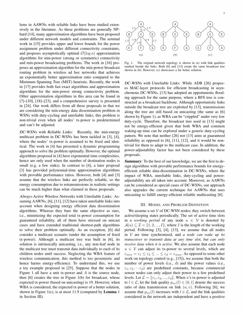
Always-Active Wireless Networks with Unreliable Links: As-suming AAWNs, [6], [11], [12] have taken unreliable links intoaccount when designing energy efficient data disseminationalgorithms. Whereas they bare the same objective as ours,i.e., minimizing the expected total tx-power consumption forguaranteed reliability, all of them have stressed on unicastcases and have extended traditional shortest-path algorithmsto solve their problem optimally. As an exception, [6] didconsider a multicast scenario (under the assumption of fixedtx-power). Although a multicast tree was built in [6], itssolution is intrinsically unicasting, i.e., any non-leaf node inthe multicast tree must transmit data individually to each of itschildren nodes until success. Neglecting the WBA feature ofwireless communication, this method is too pessimistic andhence harms energy-efficiency. To understand this, we usea toy example proposed in [25]. Suppose that the nodes inFigure 1 all have a unit tx-power and A is the source node,then [6] creates the tree in Figure 1(b) for broadcast, whoseexpected tx-power (based on unicasting) is 19. However, whenWBA is considered, the expected tx-power of a better solution,shown in Figure 1(c), is at most 11.9 (computed by Lemma 1in Section III).
B C D
E F
1/31/3
1/3
1/3 1/4 1/31/4
1/4
(a) (b) (c)
A
G
B C D
E F
A
G
B C D
E F
A
G
Fig. 1. The original network topology is shown in (a) with link qualitiesmarked beside the links. Both [6] and [13] create the same broadcast treeshown in (b). However, (c) showcases a far better solution.
DC-WSNs with Unreliable Links: While ADB [26] propos-es MAC-layer protocols for efficient broadcasting in asyn-chronous DC-WSNs, [13] has adopted an opportunistic flood-ing approach for the same purpose, where a BFS tree is con-structed as a broadcast backbone. Although opportunistic linksoutside the broadcast tree are exploited by [13], transmissionsalong the tree are still based on unicasting (the same as [6]shown by Figure 1), as WBA can be “crippled” under very lowduty-cycle. Therefore, the broadcast tree used in [13] mightnot be energy-efficient given that both WBA and commonwaking-up time can be explored under a generic duty-cyclingpattern. We note that neither [26] nor [13] aims at guaranteedreliability as opposed to [6], [11], [12], and it would be non-trivial for them to adapt to the multicast case. In addition, thepower-adjustability factor has not been considered by theseproposals.
Summary: To the best of our knowledge, we are the first to de-sign algorithms with provable performance bounds for energy-efficient reliable data-dissemination in DC-WSNs, where theimpact of WBA, unreliable links, duty-cycling and power-adjustability are all taken into account. Moreover, as AAWNscan be considered as special cases of DC-WSNs, our approachalso upgrades the current technique for AAWNs that usesunicasting to fulfill energy-efficient reliable multicasting [6].
III. MODEL AND PROBLEM DEFINITION
We assume a set V of DC-WSN nodes; they switch betweenactive/sleeping states periodically. The set of active time slotsin a working period of any node u ∈ V is denoted byA(u) ⊆ I = {1, 2, ..., I}, where I is the length of the workingperiod. Following [3], [4], [13], we assume that all nodesin V are time synchronized, and a node can wake up itstransceiver to transmit data at any time slot, but can onlyreceive data when it is active. We also assume that each nodeu ∈ V can adjust its tx-power to several levels, which areεmin = ε1 ≤ ε2 ≤ ... ≤ εd = εmax. As opposed to some otherwork on topology control (e.g., [15]), we assume that both thenumber of power levels (i.e., d) and the power values (i.e.,ε1, ε2 · · · εd) are predefined constants, because commercialsensor nodes can only adjust their power to a few predefinedlevels. Let L = {ε1, ε2, ..., εd}. When u’s tx-power is adjustedto l ∈ L, let the link quality puv(l) ∈ (0, 1] denote the successratio of data transmission on link (u, v). Following [6], weassume that puv(l) increases with l ∈ L, and the link qualitiesconsidered in the network are independent and have a positive

3
lower bound (denoted by Λ). Let Nu(l) denote the node set{v|v ∈ V\{u} ∧ puv(l) ≥ Λ}. We also assume that the linkquality puv(l) is mainly affected by the euclidian distancebetween u and v given a fixed transmission power; this impliesthat puv(l) = pvu(l), as well as v ∈ Nu(l)⇒ u ∈ Nv(l).
In a data dissemination session, there exists a source nodes ∈ V that needs to send data to a set of destination nodesR ⊆ V−{s}. Let k = |R|+1, hence the session is a broadcastif k = |V|; otherwise a multicast. A valid power assignmentfor such a session is a function L : V → L, such that when eachnode u ∈ V is adjusted to the tx-power level L(u), there existsa data dissemination tree T spanning the nodes in R ∪ {s};and the set of parent/children nodes of any node v ∈ T mustbe contained in Nv(L(v)) for v to send data and to receivecontrol messages.
To conduct a data dissemination session in a DC-WSN, weneed not only to find a valid power assignment L and a datadissemination tree T , but also to select the transmission timeslots of the forwarding nodes in T , in order to avoid trans-mitting data to sleeping nodes. Based on this observation, weprovide the definition of Viable Data-dissemination Solution(VDS) in Definition 1, where we denote the set of non-leafnodes in T by f(T ), the set of children nodes of any nodeu in T by CT (u), and the set {v|v ∈ Nu(l) ∧ t ∈ A(v)} by∂t(u, l):
Definition 1 (VDS): Suppose that T is a data disseminationtree under a valid power assignment L, and S is a functionthat satisfies:
1) For any t ∈ I and any u ∈ f(T ), S(u, t) ⊆ ∂t(u,L(u)) ∩ CT (u),
2) For any u ∈ f(T ), CT (u) ⊆⋃t∈I S(u, t),
then S is called a Viable Transmission Schedule for T and〈L, T, S〉 is called a Viable Data-dissemination Solution (VD-S).Basically, VDS requires a node u ∈ T to be responsible forsending data to nodes in the set S(u, t) at time slot t. Due tothe link unreliability, u may have to retransmit several times(in different working periods) for all the nodes in S(u, t) toreceive the data (if S(u, t) 6= ∅). To understand how manyretransmissions are needed for a forward node, we introduceLemma 1:
Lemma 1: For any node u ∈ V , any power level l ∈ L andany set Q ⊆ Nu(l), let χu(l,Q) be the random variable thatdenotes the number of transmissions by u for all the nodes inQ to receive a data packet when u’s tx-power is l. If Q 6= ∅,then we have:
E[χu(l,Q)] =∞∑i=0
[1−
∏v∈Q
(1− (1− puv(l))i)
]
Our objective is to find a VDS such that the expected totaltransmission energy of the forward nodes is minimized. Weintroduce the formal definition of this problem by Definition 2and Definition 3:
Definition 2 (Energy-Consumption Function): The energy-consumption function of a VDS 〈L, T, S〉 is
Ψ(L, T, S) =∑
u∈f(T )
∑t∈I
L(u) · χu(L(u), S(u, t)) (1)
TABLE IFREQUENTLY USED NOTATIONS
V Set of duty-cycled sensor nodess Source node for data disseminationR Set of destination nodes for data disseminationk The cardinality of R∪ {s}I Set of all time slots in a working periodA(v) Set of v’s active time slots in a working periodL Set of adjustable power levels of any nodeNv(l) Set of neighboring nodes of v when v’s tx-power
is adjusted to l∂t(v, l) Set of nodes in Nv(l) and active at time slot tf(T ) Set of non-leaf nodes in a rooted tree TCT (v) Set of the children nodes of v in rooted tree T∆ max{|Nv(l)| : v ∈ V, l ∈ L}puv(l) Quality of the link (u, v) when u’s tx-power is lγuv(l) 1− 1/ ln(1− puv(l)) if puv(l) < 1, otherwise 1γumax max{γuv(l)|l ∈ L ∧ v ∈ Nu(l)}γumin min{γuv(l)|l ∈ L ∧ v ∈ Nu(l)}χu(l,Q) Random variable denoting the number of trans-
missions by u for all the nodes in Q ⊆ Nu(l)to receive a data packet when u’s tx-power is l
Ψ(L, T, S) Energy consumption function of the viable data-dissemination solution 〈L, T, S〉
φ(L, T, S) Function used to approximate E[Ψ(L, T, S)]λ max{γu
max/γumin|u ∈ V}
ϑ(u) The Time-Reliability-Power (TRP) Set of uF Function used to map a TRP subspace to a graph
whose nodes are all in VU Union of V and the TRP sets of the nodes in V$ Weight function of any element or subset of U`(h) Length of the TRP path h〈L∗, T ∗, S∗〉 A VDS such that φ(L∗, T ∗, S∗) is minimized〈L∗, T ∗, S∗〉 A VDS such that E[Ψ(L∗, T ∗, S∗)] is minimized〈U ,WM 〉 TRP space designed for the multicast case〈U ,WB〉 TRP space designed for the broadcast case〈Lb, T b, Sb〉 Approximate solution to the ERDD problem for
the broadcast case〈Lm, Tm, Sm〉Approximate solution to the ERDD problem for
the multicast case%1(Y,W) Element closure of Y with respect to W%2(Y,W) Relationship closure of Y with respect to Win(x y) Set of the elements in the shortest TRP path from
x to y except y
Definition 3 (ERDD Problem): Given a set V of DC-WSNnodes, a source node s ∈ V , and a set of receiver nodesR ⊆ V−{s}, the Energy-efficient Reliable Data Dissemination(ERDD) problem is to find a VDS 〈L∗, T ∗, S∗〉 such thatE[Ψ(L∗, T ∗, S∗)] is minimized.As a special case of the ERDD problem, if all the networklinks are reliable and all nodes are active at all time slots,then the ERDD problem degenerates to the min-energy broad-cast/multicast problem in traditional AAWNs with perfectlinks, which is known to be NP-hard [9], [10]. Since the ERDDproblem contains a special case which is NP-hard, we have:
Theorem 1: The ERDD problem is NP-hard.In the following section, we will propose approximationalgorithms for the ERDD problem. To facilitate reading, wesummarize the notations in Table I.

4
IV. APPROXIMATION ALGORITHMS
A basic idea of our approximation algorithm design is tobuild a novel data structure called the Time-Reliability-Power(TRP) Space, where data dimensions on time, reliability andpower levels are involved to facilitate our algorithm design andanalysis. We believe that the TRP space can be used as a gen-eral data structure to facilitate the algorithm design for manyoptimization problems related to data routing/dissemination inWSNs. In the sequel, we will first introduce the concepts aboutthe TRP space, and then present our algorithms in details.
A. Time-Reliability-Power Space
To build a TRP space, we first define a positive numberγuv(l) for any u ∈ V , l ∈ L and v ∈ Nu(l) as follows:
γuv(l) =
{1− 1
ln[1−puv(l)] , puv(l) ∈ (0, 1)
1, puv(l) = 1
Note that γuv(l) is not less than 1 and decreases whenpuv(l) increases, hence a larger γuv(l) indicates a poorer link.Besides, since link qualities have a constant lower bound inpractice [6], γuv(l) has a constant upper bound. Based onthis definition, we introduce the concept of TRP space and aweight assignment method in Definition 4 and Definition 5,respectively:
Definition 4 (TRP Space): For any u ∈ V , define the TRPSet of u as ϑ(u) = {〈u, t, r, l〉|t ∈ I ∧ l ∈ L ∧ r ∈⋃v∈Nu(l){γuv(l)}}. Define U =
⋃u∈V ϑ(u) ∪ V . An access-
relationship W is any set of ordered 2-tuples wherein each2-tuple consists of two elements from U . The tuple 〈U ,W〉 iscalled a TRP space.
Definition 5 (Weight Assignment): Any x ∈ U has aweight $(x). If x ∈ V then $(x) = 0. If x = 〈u, t, r, l〉 ∈U\V , then $(x) = r · l. The weight of any Y ⊆ U is alsodenoted by $(Y) =
∑x∈Y $(x).
Intuitively, the elements in U can be viewed as weighted 4-dimensional (vector) nodes whose adjacent relationships aredetermined by an access-relationship W , while W is definedby a given problem, as we shall do in Section IV-B and IV-C.Based on above definitions, we introduce the concept of “TRPpath” in Definition 6:
Definition 6 (TRP Path): Given a TRP space 〈U ,W〉, asequence h = 〈x1, x2, ..., xm〉 is called a TRP path fromx1 to xm iff (xi, xi+1) ∈ W,∀1 ≤ i ≤ m− 1. The length ofh is defined as
`(h) =
{ ∑m−1i=2 $(xi) m > 2
0 otherwise
Based on the length function `, the shortest TRP path fromx ∈ U to y ∈ U is the one with the minimum length, whichis denoted by x y.
In our algorithm design, we will map a connected compo-nent in the TRP space 〈U ,W〉 to a data-dissemination solution.Hence, we introduce some definitions for this mapping. Thenode-image of any x ∈ U is defined as the node u ∈ V suchthat x ∈ ϑ(u)∪{u}. The edge-image of any tuple (x, y) ∈ Wis defined as the directed edge (u, v) : u ∈ V, v ∈ V such thatx ∈ ϑ(u)∪{u} and y ∈ ϑ(v)∪{v}. Suppose that 〈U1,W1〉 is
a subspace of 〈U ,W〉 (i.e., U1 ⊆ U , W1 ⊆ W), we define amapping function F such that F(U1,W1) is a directed graphconstructed by all node-images of the elements in U1 and alledge-images of the tuples in W1, i.e., all nodes in F(U1,W1)are in V .
For the convenience of description, we introduce some othernotations/definitions about the TRP space here. Given a TRPspace 〈U ,W〉 and any x, y ∈ U , we say x is accessible to y (ory is accessible from x) iff (x, y) ∈ W . Given any U1 ⊆ U , wedefine the element closure and relationship closure of U1 withrespect to W as %1(U1,W) = U1 ∪ {y|x ∈ U1 ∧ (x, y) ∈ W}and %2(U1,W) = {(x, y)|x ∈ U1 ∧ (x, y) ∈ W}, respectively.For any TRP path h = 〈x1, ..., xm〉 in 〈U ,W〉, we definein(h) = {xi|1 ≤ i ≤ m− 1}. If U1 contains all xi : 1 ≤ i ≤m, we say U1 embraces h. For any u ∈ V , define γumax =max{γuv(l)|l ∈ L ∧ v ∈ Nu(l)} and γumin = min{γuv(l)|l ∈L ∧ v ∈ Nu(l)}. Define λ = max
{γumax
γumin
∣∣u ∈ V}; it has aconstant upper bound according to the definition of γuv(l).
B. Solving ERDD for the Multicast Case
To design an approximation algorithm for the ERDD prob-lem under multicast, we construct a TRP space 〈U ,WM 〉where WM is defined by the following rules:
M1: Two elements 〈u1, t1, r1, l1〉 and 〈u2, t2, r2, l2〉 inU\V are accessible to each other iff either u1 = u2
or [u1 ∈ ∂t2(u2, l2)] ∧[u2 ∈ ∂t1(u1, l1)] ∧ [r1 ≥γu1u2(l1)] ∧ [r2 ≥ γu2u1(l2)] is true.
M2: Two elements x = 〈u1, t1, r1, l1〉 ∈ U\V and u2 ∈ Vare accessible to each other iff either u1 = u2 orthere exists y ∈ ϑ(u2) such that (x, y) ∈ WM .
u1
u2
<u1,t ,r ,l >1 1 1
<u2,t ,r ,l >2 2 2
ϑ( )u1
ϑ( )u2
......
......
Fig. 2. The link between 〈u1, t1, r1, l1〉 and 〈u2, t2, r2, l2〉 indicates thatthey are accessible to each other when rule M1 is satisfied. The other linksillustrate rule M2.
A simplified illustration of the above rules is shown inFig. 2. Note that WM is symmetric, i.e., (x, y) ∈ WM ⇒(y, x) ∈ WM . Intuitively, M1 embodies the covering relation-ship between two nodes under the time, reliability and powerconstraints, and M2 is set up to avoid counting the weightsof a multicast tree’s leaf nodes in our algorithm. Based onthis TRP space, we introduce an approximate algorithm MC-ERDD (Algorithm 1).
In Algorithm 1, we first consider 〈U ,WM 〉 as an undirectedgraph with node set U and edge set WM and find an approx-imate Node Weighted Steiner Tree (NWST) with node set U ′(line 1), then we map the NWST to an approximate solution〈Lm, Tm, Sm〉 for ERDD (lines 2-18). Roughly speaking, theidea for doing this is that we can find the tx-power and

5
Algorithm 1: MC-ERDD(V, s,R, I,U ,WM ,L,A)
1 Use an approximate node weighted Steiner treealgorithm [27] to find a subspace 〈U ′,W ′〉 of 〈U ,WM 〉which contains R∪ {s}. U ← U ′
2 Let Tm be an arbitrary spanning tree of F(U ′,W ′)3 foreach u ∈ f(Tm) do4 foreach v ∈ CTm(u) do5 if {(u′, v) ∈ WM |u′ ∈ U ′ ∩ ϑ(u)} = ∅ then6 Find 〈v, t, r, l〉 ∈ U ′\V such that u ∈ ∂t(v, l)
and r ≥ γvu(l)7 Select an arbitrary time slot t ∈ A(v) and add
〈u, t, γuv(l), l〉 into U
8 B ← CTm(u)9 foreach t ∈ I do
10 Sm(u, t)← ∅11 foreach l ∈ L do12 r ← max{r′|〈u, t, r′, l〉 ∈ U\V ∨ r′ = 0}13 Sm(u, t)← Sm(u, t) ∪ {v′|γuv′(l) ≤ r ∧ v′ ∈
B ∩ ∂t(u, l)}14 B ← B − Sm(u, t)
15 foreach node u in Tm do16 J ← the set of u’s neighboring nodes in Tm
17 l← min{l′|J ⊆ Nu(l′) ∧ l′ ∈ L}18 Lm(u)← max{l′|〈u, t′, r′, l′〉 ∈ U\V ∨ l′ = l}19 return 〈Lm, Tm, Sm〉
transmission schedule of any u ∈ f(Tm) based on the NWSTnodes in ϑ(u) (lines 8-18). To make this idea work correctly,we need to add some elements to U ′ (hence expand U ′ to U)(lines 4-7), because there may exist u ∈ f(Tm) such thatU ′ ∩ ϑ(u) = ∅ according to rule M2. The correctness andperformance ratio of Algorithm 1 will be proved in Section V.The dominating running time of Algorithm 1 is spent in line 1,which is determined by the time complexity of the NWSTalgorithm [27]. Hence, we get:
Theorem 2: The time complexity of the MC-ERDD algo-rithm is O(k2|V|2∆2).
C. Solving ERDD for the Broadcast Case
Although Algorithm 1 can also be used for broadcast, weintroduce another algorithm for the broadcast case in thissection which has a better approximation ratio. Again, thefirst step is to construct a TRP space 〈U ,WB〉, but the access-relationship WB is defined differently from WM according tothe following rules:
B1: An element 〈u1, t1, r1, l1〉 ∈ U\V is accessible to an-other element 〈u2, t2, r2, l2〉 ∈ U\V iff the Booleanexpression [u1 6= u2] ∧ [u2 ∈ ∂t1(u1, l1)] ∧ [r1 ≥γu1u2(l1)] ∧ [u1 ∈ Nu2(l2)] is true.
B2: An element x = 〈u1, t1, r1, l1〉 ∈ U\V is accessibleto u2 ∈ V iff u1 6= u2 and there exists y ∈ ϑ(u2)such that (x, y) ∈ WB .
B3: For any u ∈ V and any y ∈ ϑ(u), (u, y) ∈ WB .
u1
u2
<u1,t ,r ,l >1 1 1
<u2,t ,r ,l >2 2 2
ϑ( )u1
ϑ( )u2
......
......
Fig. 3. The directed link from z1 = 〈u1, t1, r1, l1〉 to z2 = 〈u2, t2, r2, l2〉indicates that z1 is accessible to z2 when rule B1 is satisfied. The directedlink (z1, u2) illustrates rule B2. The directed links (u1, z1) and (u2, z2)illustrate rule B3.
A simplified illustration of B1-B3 is shown in Fig. 3. Note thatWB is not symmetric and hence we cannot run Algorithm 1on 〈U ,WB〉. Actually, B1-B3 are deliberately designed withnice properties desired by our new approximation algorithmBC-ERDD (Algorithm 2), whose idea originates from theNWST algorithm in [27]. As we shall prove, by leveragingrules B1-B3, Algorithm 2 yields a better performance ratiothan Algorithm 1 in the broadcast case.
Algorithm 2: BC-ERDD(V, s, I,U ,WB ,L,A)
1 X ← ∅, Z ← V − {s}2 while |Z| > 0 do3 Find a ∈ U and a non-empty set D ⊆ Z such that
(|D| ≥ 2 ∨ a = s) = true and avl(a,D) isminimized. Let b be the node-image of a
4 A←⋃y∈D in(a y)
5 X ← A ∪X6 Z ← Z − %1(A,WB)7 if b 6= s then Z ← Z ∪ {b}8 Let T b be an arbitrary directed spanning tree ofF(%1(X,WB), %2(X,WB)) rooted at s
9 Set Lb, Sb for the nodes in T b using the same method aslines 8-18 of Algorithm 1
10 return 〈Lb, T b, Sb〉
In Algorithm 2, we use X to denote the subset of U whichwill be mapped to the forward nodes in broadcasting, and useZ to denote the set of nodes in V which are not accessiblefrom any element in X . At first, X is initialized to ∅ and Zis initialized to V − {s}. Then the algorithm uses a greedystrategy to expand X and reduce Z until Z = ∅ (lines 2-7).In each iteration, we greedily select an element a ∈ U and asubset D of U such that
avl(a,D) =$(a) +
∑y∈D `(a y)
|D|(2)
is minimized (line 3), and then update X and Z accordingly(lines 4-7). Intuitively, avl(a,D) denotes the average cost for“covering” the nodes in D, which is analogous to the “costeffectiveness” measure in the greedy set-cover algorithm [28].When X is finally determined, we use it to find an approx-imation solution 〈Lb, T b, Sb〉 in lines 8-9 based on a similar
6
mapping process as that in Algorithm 1 (regarding X as U).The time complexity of Algorithm 2 is given by:
Theorem 3: The time complexity of the BC-ERDD algo-rithm is O(|V|4∆2).
V. PERFORMANCE ANALYSIS
In this section, we prove the correctness and performanceratios of the algorithms proposed in Section IV. We shall firstintroduce an analysis method which is used for analyzing boththe MC-ERDD and the BC-ERDD algorithms, and then givethe detailed performance analysis of each algorithm.
A. A Method for Performance Analysis
From Lemma 1 and Definition 2 we can see that, forany VDS 〈L, T, S〉, the expectation value E[Ψ(L, T, S)] is asummation of infinite series, which is hard to calculate. Thismakes it hard to find the performance ratios of our algorithms.To bypass this problem, we introduce a surrogate function φ,which is defined as follows:
φ(L, T, S) =∑
u∈f(T )
∑t∈I
L(u) ·max{γuv(L(u))|v ∈ S(u, t)}
(3)It serves as an approximation to the expectation of Ψ. Let〈L, T , S〉 denote the output of Algorithm 1 or Algorithm 2.We find the quantitative relationships between φ and Ψ byLemma 2 and Lemma 3:
Lemma 2: We have E[Ψ(L, T , S)] ≤ (ln ∆+1)·φ(L, T , S)and σ[Ψ(L, T , S)] ≤
√2(ln ∆ + 1)φ(L, T , S), where σ(·)
denotes the standard deviation.Lemma 3: φ(L∗, T ∗, S∗) ≤ (1 + 1
ln 2 )λE[Ψ(L∗, T ∗, S∗)].Let 〈L∗, T ∗, S∗〉 be a VDS such that φ(L∗, T ∗, S∗) is
minimized. Intuitively, 〈L∗, T ∗, S∗〉 is a solution in whicheach forwarding node selects the more reliable links for datatransmission. Combining the above lemmas with the fact thatφ(L∗, T ∗, S∗) ≤ φ(L∗, T ∗, S∗), we immediately get:
Theorem 4: If φ(L, T , S) ≤ β · φ(L∗, T ∗, S∗), thenwe have E[Ψ(L, T , S)] ≤ αβ· E[Ψ(L∗, T ∗, S∗)] and σ[Ψ(L, T , S)] ≤
√2αβ · E[Ψ(L∗, T ∗, S∗)] where α = (1 +
1ln 2 )λ(ln ∆ + 1).
Theorem 4 actually suggests a method for analyzing ouralgorithms, i.e., to find the performance ratios of Algorithm 1and Algorithm 2, we only need to find their approximationratios with respect to the surrogate function φ. In the followingsections, we will analyze our algorithms based on this method.
B. Analyzing the MC-ERDD Algorithm
We first prove the correctness of Algorithm 1 in Lemma 4,and then prove in Lemma 5 that φ(Lm, Tm, Sm) is withinconstant times of $(U ′), which is the weight of the NWST wefound in Algorithm 1. The proofs of these lemmas are basedon the construction rules of 〈U ,WM 〉 as well as the mappingprocess employed in Algorithm 1 that maps an NWST to aVDS.
Lemma 4: 〈Lm, Tm, Sm〉 is a VDS for multicast.Lemma 5: φ(Lm, Tm, Sm) ≤ 2εmax
εmin·$(U ′)
Next, we reveal the quantitative relationship between $(U ′)and φ(L∗, T ∗, S∗) by Lemma 6. The main idea behindLemma 6 is that, we can find a tree spanning R ∪ {s}in 〈U ,WB〉 whose weight is at most (1 + λ)φ(L∗, T ∗, S∗),whereas the NWST algorithm we used in Algorithm 1 has anapproximation ratio of 2 ln k.
Lemma 6: $(U ′) ≤ 2(1 + λ) ln k · φ(L∗, T ∗, S∗)Recall that εmax, εmin are both pre-defined constants and
λ has a constant upper bound. Hence, combining Lemma 5,Lemma 6, and Theorem 4 yields:
Theorem 5: The expectation value and standard deviationof Ψ(Lm, Tm, Sm) are within 9.8η and 13.9η times ofE[Ψ(L∗, T ∗, S∗)], respectively, where η = εmax
εmin· λ(1 +
λ)(ln ∆ + 1) ln k = O(ln ∆ ln k).
C. Analyzing the BC-ERDD Algorithm
Based on similar reasoning to the proof of Lemma 4, wecan also prove the correctness of Algorithm 2 based on thedefinition of WB , as shown by Lemma 7:
Lemma 7: 〈Lb, T b, Sb〉 is a VDS for broadcast.Suppose that the while loop in lines 2-7 of Algorithm 2executes for q times. Let Zj = Z and Xj = X after thejth while loop is executed. Let Dj be the set D found in thejth while loop. Clearly we have $(X0) = 0 and |Zq| = 0.Indeed, the value ($(Xj+1)−$(Xj))/|Dj+1| represents the“cost effectiveness” of the elements added to X in the (j+1)thloop, which is bounded by Lemma 8:
Lemma 8: ($(Xj+1) − $(Xj)) · |Zj | ≤ |Dj+1| · φ(L∗,
T ∗, S∗)(0 ≤ j ≤ q − 1)Note that the elements in Xq are finally mapped to thetransmission schedules of the non-leaf nodes in T b. Hence,based on Lemma 8 and the mapping process in Algorithm 2,we can get:
Lemma 9: φ(Lb, T b, Sb) ≤ εmax
εmin· (2 ln k + 1) ·
φ(L∗, T ∗, S∗)Combining Lemma 9 with Theorem 4, we get:
Theorem 6: The expectation value and standard devia-tion of Ψ(Lb, T b, Sb) are within 2.5µ and 3.5µ times ofE[Ψ(L∗, T ∗, S∗)], respectively, where µ = εmax
εminλ(ln ∆ +
1)(2 ln k + 1) = O(ln ∆ ln k).
D. The Price of Power Adjustability and Link Reliability
Having shown that involving more parameters in a data dis-semination problem does not affect the approximability of theproblem, we do need to pay a price in terms of the coefficientshidden behind the O-notation. Fortunately, we shall show thatthis price is acceptable given the actual parameters suggestedby the real-life WSNs. Taking the CC2520 RF transceiver [29](the most up-to-date radio interface of a sensor node) asan example, it offers 9 tx-power levels between (-18)dBmand 5dBm, but the most usable levels lie between (-7)dBmand 5dBm (as a very low tx-power leads to unstable linkperformance easily affected by ambient interference from, forexample, WiFi transmissions). This suggests that εmax
εmin≈ 15.8
in practice. Moreover, the link quality lower bound Λ is oftendecided by a WSN routing protocol, in a way that a link whose
7
10 30 50 70 900
1000
2000
3000
4000
5000
6000
7000
Number of Destination Nodes
To
tal T
x−
Po
we
r C
on
su
mp
tio
n (
mW
)
MEERMRL−W
MC−ERDD
MEERMRL
(a) |V|=100
20 60 100 140 1800
2000
4000
6000
8000
10000
12000
Number of Destination Nodes
To
tal T
x−
Po
we
r C
on
su
mp
tio
n (
mW
)
MEERMRL−W
MC−ERDD
MEERMRL
(b) |V|=200
Fig. 4. MC-ERDD vs. MEERMRL
10 30 50 70 900
1000
2000
3000
4000
5000
6000
Number of Destination Nodes
To
tal T
x−
Po
we
r C
on
su
mp
tio
n (
mW
)
TCS
MC−ERDD
(a) |V|=100
20 60 100 140 1800
2000
4000
6000
8000
10000
12000
Number of Destination Nodes
To
tal T
x−
Po
we
r C
on
su
mp
tio
n (
mW
)
TCS
MC−ERDD
(b) |V|=200
Fig. 5. MC-ERDD vs. TCS
0.75 0.8 0.85 0.9 0.95 1
2000
3000
4000
5000
6000
7000
8000
9000
Packet Delivery Ratio
To
tal T
x−
Po
we
r C
on
su
mp
tio
n (
mW
)
OF
BC−ERDD
(a) |V|=100
0.75 0.8 0.85 0.9 0.95 1
0.4
0.6
0.8
1
1.2
1.4
1.6
1.8x 10
4
Packet Delivery Ratio
To
tal T
x−
Po
we
r C
on
su
mp
tio
n (
mW
)
OF
BC−ERDD
(b) |V|=200
Fig. 6. BC-ERDD vs. OF
quality is below Λ is not used in carrying data traffic. Whereasthe value of Λ depends on a specific protocol, the fact that λ isa logarithmic function of link quality implies that its value canbe negligible. For example, the value of λ is only increasedfrom 1.62 to 5.48 if Λ is reduced by 4 times from 0.8 to 0.2.
VI. PERFORMANCE EVALUATION
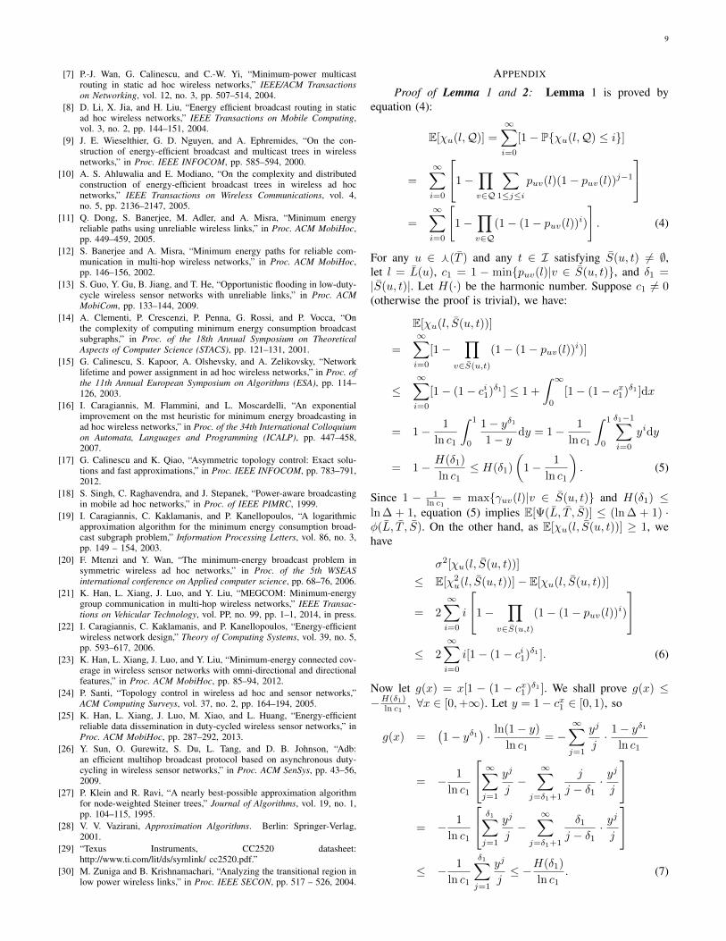
We conduct extensive simulations to evaluate the perfor-mance of our algorithms. In the simulations, we randomlydeploy |V| nodes in a square of 102|V|m2 and set themaximum tx-power (εmax) to 15.0dBm as that in [6]. Thesource/destination nodes are randomly selected in V . Follow-ing [13], the link qualities are set by considering the path losschannels and shadowing effects [30]. All the reported data inour figures are the average of 50 simulation results.
We compare our algorithms with three representativealgorithms in the literature: (1) The multicast algorithm(MEERMRL) proposed by [6] for AAWNs; (2) The mul-ticast algorithm (TCS) proposed in [3] for DC-WSNs withperfectly reliable links; (3) The broadcast algorithm (Oppor-tunistic Flooding, or OF) proposed in [13] for DC-WSNswith unreliable links. Since all these algorithms require afixed tx-power, we fix the tx-power of all nodes to 15.0dBmwhen comparing with them. For fairness sake, we apply thesimple node-coloring based collision-free scheduling schemeproposed by [3] to all the algorithms except OF, which usesa backoff scheme to avoid collisions [13].
In Figure 4, we compare MC-ERDD (Algorithm 1) withthe MEERMRL algorithm, where nodes are set always-active.
The number of network nodes is set to 100 and 200 inFigure 4(a) and Figure 4(b), respectively, and the percentage ofdestination nodes scales from 10% to 90% with an incrementof 20%. Though multicast is implemented by unicast in [6], wealso implement an adapted version of MEERMRL (denoted byMEERMRL-W) that leverages WBA for multicasting but stillapplies the same multicast tree that MEERMRL constructs.It can be seen from Figure 4 that MC-ERDD outperformsboth MEERMRL and MEERMRL-W significantly, which canbe explained by the reason that WBA is neglected when theMEERMRL multicast tree is constructed in [6].
In Figure 5, we compare MC-ERDD with the TCS algo-rithm. Nodes are duty-cycled for both cases, with the lengthof working period set to 20. Each node may have at most10 active time slots within a working period (50% duty-cycle ratio) and these slots are randomly selected. MC-ERDD(again) significantly outperforms TCS, simply because TCSis only duty-cycle-aware but not link-quality-aware, it hencemay select poor links for data transmission, resulting in higherenergy consumption for guaranteeing reliability.
In Figure 6, we compare BC-ERDD (Algorithm 2) with theOF algorithm for broadcasting, where the duty-cycle setting isthe same as that in Figure 5. The parameters for implementingOF are based on the experimental results reported in [13],i.e., we set lth = 0.9 and p = 0.5, in order to obtainthe best performance of OF. Following the testing methodin [13], we scale the packet delivery ratio PDR from 75% to99%, and record the total tx-power consumption when certainPDR is attained. It can be seen that BC-ERDD outperforms

8
OF significantly regardless of the attainable PDR, althoughopportunistic links are exploited in OF to reduce the energyconsumption. Both results in Figure 4 and 6 suggest that, forthe sake of energy efficiency, WBA is better to be taken intoaccount at the tree construction phase; any “patching” aftera WBA-oblivious tree construction may not achieve the bestperformance. Also, OF constructs its broadcast tree regardlessof nodes’ duty cycling, which further degrades its performancein general DC-WSNs.
As OF is designed for WSNs with very low duty-cycle, wefurther compare BC-ERDD with OF under different Duty-Cycle Ratios (DCRs) in Figure 7, where we set |V| = 100,|I| = 20 and fix the PDR to 99%. We scale nodes’ maximumnumber of active time slots within a working period from2 to 10 with an increment of 2, hence the DCR variesfrom 10% to 50%. As expected, BC-ERDD outperforms OFunder all these ratios, although the advantage of BC-ERDD ismore conspicuous under higher ratios, as WBA becomes lesssignificant if nodes sleep most of the time under low DCRs.
2 3 4 5 6 7 8 9 10
4500
5000
5500
6000
6500
7000
7500
8000
8500
Active time slots
To
tal T
x−
Po
we
r C
on
su
mp
tio
n (
mW
)
OF
BC−ERDD
Fig. 7. BC-ERDD vs. OF under different duty-cycle ratios.
Finally, we study the impact of power-adjustability onenergy consumption. Since we are not aware of any othermulticast/broadcast algorithms for DC-WSNs with power-adjustability, we study only our own algorithms in Figure 8,where Figure 8(a) is for MC-ERDD and Figure 8(b) is forBC-ERDD. We use “FIXED” to denote the case where eachnode’s tx-power is fixed to 15.0dBm, and use “ADJUST” todenote the case where each node can adjust its tx-power tothree levels, namely 11.0dBm, 13.0dBm and 15.0dBm. Thenumber of network nodes in Figure 8 is set to 100, andnodes are duty-cycled as that in Figure 5 and Figure 6. Itcan seen from Figure 8 that introducing power-adjustabilitycan significantly improve energy-efficiency, because nodes canuse lower tx-power to communicate with nearer nodes, hencereducing energy consumption.
VII. CONCLUSION
We have studied the energy-efficient reliable data dissemi-nation problem in DC-WSNs with unreliable links. We seekto minimize the total expected tx-power consumption forreliable multicasting/broadcasting. Due to the NP-hardness ofthe problem, we have proposed approximation algorithms withprovable performance ratios based on a novel data structure
10 30 50 70 900
500
1000
1500
2000
2500
3000
3500
4000
4500
Number of Destination Nodes
Tota
l T
x−
Pow
er
Consum
ption (
mW
)
ADJUST
FIXED
(a) MC-ERDD
0.75 0.8 0.85 0.9 0.95 1
1000
1500
2000
2500
3000
3500
4000
4500
5000
5500
Packet Delivery RatioT
ota
l T
x−
Pow
er
Consum
ption (
mW
)
ADJUST
FIXED
(b) BC-ERDD
Fig. 8. Studying the impact of power-adjustability.
named as Time-Reliability-Power space. To the best of ourknowledge, these algorithms are, on the one hand, the firstto holistically take into account various aspects includingduty-cycling, wireless broadcast advantage, unreliable linksand power-adjustability, and on the other hand, to provideguaranteed performance bounds for energy-efficient reliabledata dissemination in DC-WSNs. In addition to the theoreticalcontribution, our extensive simulation results also demonstratethe practical efficiency of our algorithms, by comparing withrepresentative proposals in the literature.
REFERENCES
[1] Q. Wang, Y. Zhu, and L. Cheng, “Reprogramming wireless sensornetworks: challenges and approaches,” IEEE Network, vol. 20, no. 3,pp. 48–55, 2006.
[2] S. Kulkarni and L. Wang, “Energy-efficient multihop reprogramming forsensor networks,” ACM Transactions on Sensor Networks, vol. 5, no. 2,pp. 1–40, 2009.
[3] K. Han, Y. Liu, and J. Luo, “Duty-cycle-aware minimum-energy mul-ticasting in wireless sensor networks,” IEEE/ACM Transactions onNetworking, vol. 21, no. 3, pp. 910–923, 2013.
[4] L. Su, B. Ding, Y. Yang, T. F. Abdelzaher, G. Cao, and J. C. Hou,“Ocast: optimal multicast routing protocol for wireless sensor networks,”in Proc. IEEE ICNP, pp. 151–160, 2009.
[5] K. Han, J. Luo, Y. Liu, and A. Vasilakos, “Algorithm design for datacommunications in duty-cycled wireless sensor networks: a survey,”IEEE Communications Magazine, vol. 51, no. 7, pp. 107–113, 2013.
[6] X. Y. Li, Y. Wang, H. Chen, X. Chu, Y. Wu, and Y. Qi, “Reliable andenergy-efficient routing for static wireless ad hoc networks with unre-liable links,” IEEE Transactions on Parallel and Distributed Systems,vol. 20, no. 10, pp. 1408–1421, 2009.
9
[7] P.-J. Wan, G. Calinescu, and C.-W. Yi, “Minimum-power multicastrouting in static ad hoc wireless networks,” IEEE/ACM Transactionson Networking, vol. 12, no. 3, pp. 507–514, 2004.
[8] D. Li, X. Jia, and H. Liu, “Energy efficient broadcast routing in staticad hoc wireless networks,” IEEE Transactions on Mobile Computing,vol. 3, no. 2, pp. 144–151, 2004.
[9] J. E. Wieselthier, G. D. Nguyen, and A. Ephremides, “On the con-struction of energy-efficient broadcast and multicast trees in wirelessnetworks,” in Proc. IEEE INFOCOM, pp. 585–594, 2000.
[10] A. S. Ahluwalia and E. Modiano, “On the complexity and distributedconstruction of energy-efficient broadcast trees in wireless ad hocnetworks,” IEEE Transactions on Wireless Communications, vol. 4,no. 5, pp. 2136–2147, 2005.
[11] Q. Dong, S. Banerjee, M. Adler, and A. Misra, “Minimum energyreliable paths using unreliable wireless links,” in Proc. ACM MobiHoc,pp. 449–459, 2005.
[12] S. Banerjee and A. Misra, “Minimum energy paths for reliable com-munication in multi-hop wireless networks,” in Proc. ACM MobiHoc,pp. 146–156, 2002.
[13] S. Guo, Y. Gu, B. Jiang, and T. He, “Opportunistic flooding in low-duty-cycle wireless sensor networks with unreliable links,” in Proc. ACMMobiCom, pp. 133–144, 2009.
[14] A. Clementi, P. Crescenzi, P. Penna, G. Rossi, and P. Vocca, “Onthe complexity of computing minimum energy consumption broadcastsubgraphs,” in Proc. of the 18th Annual Symposium on TheoreticalAspects of Computer Science (STACS), pp. 121–131, 2001.
[15] G. Calinescu, S. Kapoor, A. Olshevsky, and A. Zelikovsky, “Networklifetime and power assignment in ad hoc wireless networks,” in Proc. ofthe 11th Annual European Symposium on Algorithms (ESA), pp. 114–126, 2003.
[16] I. Caragiannis, M. Flammini, and L. Moscardelli, “An exponentialimprovement on the mst heuristic for minimum energy broadcasting inad hoc wireless networks,” in Proc. of the 34th International Colloquiumon Automata, Languages and Programming (ICALP), pp. 447–458,2007.
[17] G. Calinescu and K. Qiao, “Asymmetric topology control: Exact solu-tions and fast approximations,” in Proc. IEEE INFOCOM, pp. 783–791,2012.
[18] S. Singh, C. Raghavendra, and J. Stepanek, “Power-aware broadcastingin mobile ad hoc networks,” in Proc. of IEEE PIMRC, 1999.
[19] I. Caragiannis, C. Kaklamanis, and P. Kanellopoulos, “A logarithmicapproximation algorithm for the minimum energy consumption broad-cast subgraph problem,” Information Processing Letters, vol. 86, no. 3,pp. 149 – 154, 2003.
[20] F. Mtenzi and Y. Wan, “The minimum-energy broadcast problem insymmetric wireless ad hoc networks,” in Proc. of the 5th WSEASinternational conference on Applied computer science, pp. 68–76, 2006.
[21] K. Han, L. Xiang, J. Luo, and Y. Liu, “MEGCOM: Minimum-energygroup communication in multi-hop wireless networks,” IEEE Transac-tions on Vehicular Technology, vol. PP, no. 99, pp. 1–1, 2014, in press.
[22] I. Caragiannis, C. Kaklamanis, and P. Kanellopoulos, “Energy-efficientwireless network design,” Theory of Computing Systems, vol. 39, no. 5,pp. 593–617, 2006.
[23] K. Han, L. Xiang, J. Luo, and Y. Liu, “Minimum-energy connected cov-erage in wireless sensor networks with omni-directional and directionalfeatures,” in Proc. ACM MobiHoc, pp. 85–94, 2012.
[24] P. Santi, “Topology control in wireless ad hoc and sensor networks,”ACM Computing Surveys, vol. 37, no. 2, pp. 164–194, 2005.
[25] K. Han, L. Xiang, J. Luo, M. Xiao, and L. Huang, “Energy-efficientreliable data dissemination in duty-cycled wireless sensor networks,” inProc. ACM MobiHoc, pp. 287–292, 2013.
[26] Y. Sun, O. Gurewitz, S. Du, L. Tang, and D. B. Johnson, “Adb:an efficient multihop broadcast protocol based on asynchronous duty-cycling in wireless sensor networks,” in Proc. ACM SenSys, pp. 43–56,2009.
[27] P. Klein and R. Ravi, “A nearly best-possible approximation algorithmfor node-weighted Steiner trees,” Journal of Algorithms, vol. 19, no. 1,pp. 104–115, 1995.
[28] V. V. Vazirani, Approximation Algorithms. Berlin: Springer-Verlag,2001.
[29] “Texus Instruments, CC2520 datasheet:http://www.ti.com/lit/ds/symlink/ cc2520.pdf.”
[30] M. Zuniga and B. Krishnamachari, “Analyzing the transitional region inlow power wireless links,” in Proc. IEEE SECON, pp. 517 – 526, 2004.
APPENDIX
Proof of Lemma 1 and 2: Lemma 1 is proved byequation (4):
E[χu(l,Q)] =∞∑i=0
[1− P{χu(l,Q) ≤ i}]
=∞∑i=0
1−∏v∈Q
∑1≤j≤i
puv(l)(1− puv(l))j−1
=
∞∑i=0
[1−
∏v∈Q
(1− (1− puv(l))i)
]. (4)
For any u ∈ f(T ) and any t ∈ I satisfying S(u, t) 6= ∅,let l = L(u), c1 = 1 − min{puv(l)|v ∈ S(u, t)}, and δ1 =|S(u, t)|. Let H(·) be the harmonic number. Suppose c1 6= 0(otherwise the proof is trivial), we have:
E[χu(l, S(u, t))]
=∞∑i=0
[1−∏
v∈S(u,t)
(1− (1− puv(l))i)]
≤∞∑i=0
[1− (1− ci1)δ1 ] ≤ 1 +
∫ ∞0
[1− (1− cx1)δ1 ]dx
= 1− 1
ln c1
∫ 1
0
1− yδ11− y
dy = 1− 1
ln c1
∫ 1
0
δ1−1∑i=0
yidy
= 1− H(δ1)
ln c1≤ H(δ1)
(1− 1
ln c1
). (5)
Since 1 − 1ln c1
= max{γuv(l)|v ∈ S(u, t)} and H(δ1) ≤ln ∆ + 1, equation (5) implies E[Ψ(L, T , S)] ≤ (ln ∆ + 1) ·φ(L, T , S). On the other hand, as E[χu(l, S(u, t))] ≥ 1, wehave
σ2[χu(l, S(u, t))]
≤ E[χ2u(l, S(u, t))]− E[χu(l, S(u, t))]
= 2∞∑i=0
i
1−∏
v∈S(u,t)
(1− (1− puv(l))i)
≤ 2
∞∑i=0
i[1− (1− ci1)δ1 ]. (6)
Now let g(x) = x[1 − (1 − cx1)δ1 ]. We shall prove g(x) ≤−H(δ1)
ln c1, ∀x ∈ [0,+∞). Let y = 1− cx1 ∈ [0, 1), so
g(x) =(1− yδ1
)· ln(1− y)
ln c1= −
∞∑j=1
yj
j· 1− yδ1
ln c1
= − 1
ln c1
∞∑j=1
yj
j−
∞∑j=δ1+1
j
j − δ1· y
j
j
= − 1
ln c1
δ1∑j=1
yj
j−
∞∑j=δ1+1
δ1j − δ1
· yj
j
≤ − 1
ln c1
δ1∑j=1
yj
j≤ −H(δ1)
ln c1. (7)

10
Using (6) and (7), we get
σ2[χu(l, S(u, t))]
≤ −2H(δ1)
ln c1+ 2
∫ ∞0
g(x)dx
= −2H(δ1)
ln c1− 2
∫ 1
0
ln(1− y)
ln2 c1
δ1−1∑j=0
yjdy. (8)
Meanwhile, we have
∫ 1
0
ln(1− y)
δ1−1∑j=0
yjdy
=
δ1−1∑j=0
1
j + 1
∫ 1
0
((j + 1)yj ln(1− y) +
j∑i=0
yi
)dy
−δ1−1∑j=0
1
j + 1
∫ 1
0
j∑i=0
yidy
=
δ1−1∑j=0
1
j + 1
[(yj+1 − 1) ln(1− y)
∣∣10−H(j + 1)
]
= −δ1∑j=1
H(j)
j. (9)
Plugging (9) into (8) gives us
σ2[χu(l, S(u, t))]
≤ −2H(δ1)
ln c1+
2
ln2 c1
δ1∑j=1
H(j)
j
≤ 2H2(δ1) ·(
1− 1
ln c1
)2
≤ 2(ln ∆ + 1)2 ·max2{γuv(l)|v ∈ S(u, t)}. (10)
As the random variables in {χu(L(u), S(u, t))|u ∈ f(T ), t ∈I} are mutually independent, using (10) we have
σ2[Ψ(L, T , S)]
≤
∑u∈f(T )
∑t∈I
L(u) · σ[χu(L(u), S(u, t))
]2
≤ [√
2(ln ∆ + 1)φ(L, T , S)]2,
hence σ[Ψ(L, T , S)] ≤√
2(ln ∆ + 1)φ(L, T , S).Proof of Lemma 3: For any u ∈ f(T ∗) and any
t ∈ I satisfying S∗(u, t) 6= ∅, let l∗ = L∗(u), c2 =1−max{puv(l∗)|v ∈ S∗(u, t)} and δ2 = |S∗(u, t)|. Supposec2 6= 0 (otherwise the proof becomes trivial), we have:
min{γuv(l∗)|v ∈ S∗(u, t)} ≥ γumin≥ γumax
λ≥ 1
λ·max{γuv(l∗)|v ∈ S∗(u, t)}. (11)
Since 1− 1ln c2
= min{γuv(l∗)|v ∈ S∗(u, t)}, we get
E[χu(l∗, S∗(u, t))]
=∞∑i=0
1−∏
v∈S∗(u,t)
(1− (1− puv(l∗))i)
≥
∞∑i=0
[1− (1− ci2)δ2 ] ≥∫ ∞
0
1− (1− cx2)δ2dx
= −H(δ2)
ln c2≥ − ln(δ2 + 1)
ln c2≥ ln 2 · (min{γuv(l∗)|v ∈ S∗(u, t)} − 1) (12)
Using (11), (12) and E[χu(l∗, S∗(u, t))] ≥ 1, we have
(1 + ln 2)E[Ψ(L∗, T ∗, S∗)] ≥ ln 2
λ· φ(L∗, T ∗, S∗).
Hence the lemma follows.Proof of Lemma 4: Let us call the edge-images of the 2-
tuples constructed by rules M1 and M2 the “M1-edges” andthe “M2-edges”, respectively. For ∀u ∈ f(Tm) and ∀v ∈CTm(u), we have:(1) If {(u′, v) ∈ WM |u′ ∈ U ′ ∩ ϑ(u)} = ∅, then (u, v)must be a M2-edge. According to M2, we can always finda satisfactory 〈v, t, r, l〉 in line 6. Hence there exists t ∈ A(v)such that v ∈ ∂t(u, l) and v ∈ Sm(u, t) according to lines 6-7and lines 12-13 of Algorithm 1.(2) If {(u′, v) ∈ WM |u′ ∈ U ′ ∩ ϑ(u)} 6= ∅, then (u, v) canbe a M1-edge or a M2-edge. In either case, there must existan element 〈u, t, r′, l〉 ∈ U ′\V such that v ∈ ∂t(u, l) and r′ ≥γuv(l). Hence, we can know v ∈
⋃t∈I S
m(u, t) according tolines 12-13 of Algorithm 1.
The above reasoning actually proves CTm(u) ⊆⋃t∈I
Sm(u, t) for any u ∈ f(Tm). Other conditions for〈Lm, Tm, Sm〉 to be a VDS can be proved similarly basedon rules M1 and M2. Hence the lemma follows.
Proof of Lemma 5: Let K(u, t) = {〈u, t, r′, l′〉 ∈ U}.According to lines 8-18 of Algorithm 1, for any u ∈ f(Tm),t ∈ I and any v ∈ Sm(u, t) 6= ∅, there must exist〈u, t, r, l〉 ∈ U such that l ≤ Lm(u) and γuv(l) ≤ r. Hencewe get γuv(Lm(u)) ≤ γuv(l) ≤ r ≤ $(〈u, t, r, l〉)/εminand max{γuv(Lm(u))|v ∈ Sm(u, t)} ≤ $(K(u, t))/εmin.Therefore
φ(Lm, Tm, Sm) ≤∑
u∈f(Tm)
∑t∈I
Lm(u) ·$(K(u, t))/εmin
≤ εmaxεmin
·$(U).
Note that any two different nodes u ∈ V and v ∈ V cannotbe adjacent in the TRP space. Besides, rules M1-M2 implythat when u is adjacent to certain element y ∈ ϑ(v), theremust exist a symmetric x ∈ ϑ(u) which has the same weightas y. Therefore, from lines 4-14 of Algorithm 1 we knowthat the total weight of the elements in U\U ′ is no more thanthat of U ′ after Algorithm 1 finishes. Hence, it follows that$(U) ≤ 2 ·$(U ′) and the lemma is proved.
Proof of Lemma 6: Let W1 = R ∪ {s} ∪ {〈u, t, r, l〉|u ∈ f(T ∗) ∧ t ∈ I ∧ l = L∗(u) ∧ S∗(u, t) 6= ∅ ∧ [r =
11
max{γuv(l)|v ∈ S∗(u, t)}]}. Clearly we have $(W1) =φ(L∗, T ∗, S∗).
Initialize W2 to the empty set, and then we check eachv ∈ f(T ∗)\{s}. Suppose that the parent node of v is u. Since〈L∗, T ∗, S∗〉 is a VDS, we can find y1 = 〈u, t1, r1, l1〉 ∈W1 and y2 = 〈v, t2, r2, l2〉 ∈ W1 such that v ∈ ∂t1(u, l1),r1 ≥ γuv(l1) and u ∈ Nv(l2). Let t3 be an arbitrary timeslot in A(u) and we add y3 = 〈v, t3, γvu(l2), l2〉 into W2.Note that y1 and y3 are accessible to each other according toM1, and $(y3) is no more than λ ·$(y2). After all the nodesin f(T ∗)\{s} are checked, $(W2) is at most λ · $(W1).Moreover, for any pair of nodes in R ∪ {s}, there exists aTRP path between them which is embraced by W1 ∪W2.
Suppose that the weight of an optimal NWST spanningR ∪ {s} in the TRP space 〈U ,WM 〉 is W ∗. Since theapproximation ratio of the NWST algorithm used in line 1of Algorithm 1 is 2 ln k [27], we get
$(U ′) ≤ 2 ln k ·W ∗ ≤ 2 ln k ·$(W1 ∪W2)
≤ 2 ln k · (1 + λ) ·$(W1)
= 2 ln k · (1 + λ) · φ(L∗, T ∗, S∗).
Hence the lemma followsProof of Lemma 7: According to line 8 of Algorithm 2,
it can be seen that T b is a broadcast tree in G rooted at s.Next, we prove that Lb and Sb are valid for T b. We notethat, for any u ∈ f(T b) and any v ∈ CT b(u), there mustexist 〈u, t1, r1, l1〉 ∈ X and 〈v, t2, r2, l2〉 ∈ ϑ(v) such that(〈u, t1, r1, l1〉, 〈v, t2, r2, l2〉) ∈ WB according to rules B1 andB2. This implies v ∈ ∂t1(u, l1), r1 ≥ γuv(l1) and u ∈ Nv(l2).Based on this observation and line 9 of Algorithm 2, it canbe proved that ∀t ∈ I : Sb(u, t) ⊆ ∂t(u, Lb(u))∩CT b(u) andCT b(u) ⊆
⋃t∈I S
b(u, t) using a similar reasoning with thatin the proof of Lemma 4. Hence the lemma follows.
Proof of Lemma 8: Let the path from s to any z ∈ Zjin T ∗ be 〈u1, u2, ..., um〉 where u1 = s and um = z. For∀1 ≤ i < m, we can find xi = 〈ui, ti, ri, li〉 such that ti ∈ I,ui+1 ∈ S∗(ui, ti), li = L∗(ui) and ri = max{γuiv(li)|v ∈S∗(ui, ti)}. Let Pz = {s, x1, x2, ...xm−1, z}. According tothe construction rules of WB , we know that there exists P ⊆⋃z∈Zj
Pz such that P embraces a TRP path from s to anyz ∈ Zj and $(P ) ≤ φ(L∗, T ∗, S∗). Then, using a similarmethod as the “spider decomposition” method in [27], P canbe partitioned into subsets P 1, ..., Pw such that if P i∩Zj 6= ∅,then P i embraces disjoint TRP paths from certain rt i ∈ P ito the nodes in P i ∩ Zj(1 ≤ i ≤ w). Based on line 3 ofAlgorithm 2 we know that, if P i ∩ Zj 6= ∅, then
$(Xj+1)−$(Xj)
|Dj+1|≤ avl(rt i, P i ∩ Zj) (1 ≤ i ≤ w) (13)
Combining (13) with
w∑i=1
avl(rt i, P i ∩ Zj) · |P i ∩ Zj | ≤ $(P ) ≤ φ(L∗, T ∗, S∗)
(14)and
∑wi=1 |P i ∩ Zj | = |Zj |, the lemma follows.
Proof of Lemma 9: From lines 3-7 of Algorithm 2 weknow that
|Zj | − |Zj+1| ≥ max{|Dj+1| − 1, 1}, (0 ≤ j ≤ q − 1) (15)
Combining (15) and Lemma 8 yields:
|Zj+1| ≤
[1− $(Xj+1)−$(Xj)
2φ(L∗, T ∗, S∗)
]|Zj |, (0 ≤ j ≤ q − 1)
Using this and ln(1 + x) ≤ x, we have
ln |Zj | − ln |Zj+1| ≥$(Xj+1)−$(Xj)
2φ(L∗, T ∗, S∗), (0 ≤ j ≤ q − 2)
(16)Since $(X0) = 0, |Zq−1| ≥ 1 and |Z0| ≤ k, we get
$(Xq−1) ≤ 2(ln |Z0| − ln |Zq−1|) · φ(L∗, T ∗, S∗)
≤ 2 ln k · φ(L∗, T ∗, S∗). (17)
Moreover, using |Dj+1| ≤ |Zj |(0 ≤ j ≤ q−1) and Lemma 8,we know $(Xq)−$(Xq−1) ≤ φ(L∗, T ∗, S∗). Combining thisfact with (17), we immediately get
$(Xq) ≤ (2 ln k + 1) · φ(L∗, T ∗, S∗). (18)
Finally, according to lines 8-9 of Algorithm 2 we know that,for ∀u ∈ f(T b), ∀t ∈ I and ∀v ∈ Sb(u, t) 6= ∅, theremust exist certain element 〈u, t, r, l〉 ∈ Xq ∩ ϑ(u) such thatγuv(L
b(u)) ≤ γuv(l) ≤ r. Hence
φ(Lb, T b, Sb)
=∑
u∈f(T b)
∑t∈I
Lb(u) ·max{γuv(Lb(u))|v ∈ Sb(u, t)}
≤∑
u∈f(T b)
∑t∈I
Lb(u) ·$({〈u, t, r′, l′〉 ∈ Xq})/εmin
≤ εmaxεmin
·$(Xq). (19)
The lemma then follows by combining (18) and (19).Proof of Theorem 2: The time complexity of the NWST
algorithm proposed in [27] is O(k2n2) and n = |U| in ourcase. Since |U| ≤ |V||L||I|∆ where |L| and |I| are bothpredefined constants, the time complexity of Algorithm 1 isO(k2|U|2) = O(k2|V|2∆2).
Proof of Theorem 3: Algorithm 2 has its running timepredominantly spent on line 3, which can be implemented asfollows. For any u ∈ U , we first order the nodes in Z to〈z1, z2, ..., z|Z|〉 such that `(u zi) ≤ `(u zi+1)(1 ≤i < |Z|), then we find 1 ≤ m ≤ |Z| such that avl(u,Du) isminimized, where Du = {z1, z2, ..., zm}. Hence, avl(a,D) =min{avl(u,Du)|u ∈ U} and finding (a,D) costs O(k|U|2)= O(k3∆2) time if Dijkstra’s algorithm is used. Since line 3runs for at most k times, the time complexity of Algorithm 2is O(k4∆2) = O(|V|4∆2).

12
Kai Han received the B.S. and Ph.D. degrees incomputer science from the University of Scienceand Technology of China, Hefei, China, in 1997and 2004, respectively. From 2005 to 2008, he wasa post-doctoral research fellow at the School ofMathematics, University of Science and Technologyof China.
He is currently an associate professor at theSchool of Computer Science, Zhongyuan Universityof Technology, China. This work is done when heworks as a visiting fellow at the School of Computer
Engineering, Nanyang Technological University, Singapore. His researchinterests include wireless ad hoc and sensor networks, social networks,combinatorial and stochastic optimization, machine learning theory, as wellas algorithmic game theory. He is a Member of both IEEE and ACM.
Jun Luo got his PhD degree in computer sciencefrom EPFL (Swiss Federal Institute of Technologyin Lausanne), Lausanne, Switzerland, in 2006. From2006 to 2008, he has worked as a post-doctoralresearch fellow in the Department of Electricaland Computer Engineering, University of Waterloo,Waterloo, Canada. In 2008, he joined the facultyof the School of Computer Engineering, NanyangTechnological University in Singapore, where heis currently an Assistant Professor. His researchinterests include wireless networking, distributed
systems, multimedia protocols, network modeling and performance analysis,applied operations research, as well as network security. He is a Member ofboth IEEE and ACM.
Liu Xiang received the B.S. degree in Electron-ic Engineering from Tsinghua University, Beijing,China, and the Ph.D. degree in Computer Sciencefrom Nanyang Technological University, Singapore.She is currently a research scientist with Institutefor Infocomm Research (I2R), A*STAR, Singapore.Her research interests include network modelling,analysis, and optimization for wireless networks andsmart grid.
Mingjun Xiao is an associate professor in theSchool of Computer Science and Technology atthe University of Science and Technology of China(USTC). He received his Ph.D. degree from USTC in2004. In 2012, he was a visiting scholar at TempleUniversity. He has served as a reviewer for manyjournal papers. His main research interests includewireless sensor networks, delay tolerant networksand mobile social networks.
Liusheng Huang is a professor in the School ofComputer Science and Technology at the Universityof Science and Technology of China. He received hisM.S. degree in computer science from the Universityof Science and Technology of China in 1988. Heserves on the editorial board of many journals. Hehas published 6 books, and more than 200 papers.His main research interests include wireless sensornetworks, delay tolerant networks and Internet ofthings.