Embed Size (px)
Citation preview
AC/DC MODULE
V E R S I O N 3 . 4
USER’S GUIDE COMSOL Multiphysics

How to contact COMSOL:
BeneluxCOMSOL BV Röntgenlaan 19 2719 DX Zoetermeer The Netherlands Phone: +31 (0) 79 363 4230 Fax: +31 (0) 79 361 [email protected] www.femlab.nl
Denmark COMSOL A/S Diplomvej 376 2800 Kgs. Lyngby Phone: +45 88 70 82 00 Fax: +45 88 70 80 90 [email protected] www.comsol.dk
Finland COMSOL OY Arabianranta 6FIN-00560 Helsinki Phone: +358 9 2510 400 Fax: +358 9 2510 4010 [email protected] www.comsol.fi
France COMSOL France WTC, 5 pl. Robert Schuman F-38000 Grenoble Phone: +33 (0)4 76 46 49 01 Fax: +33 (0)4 76 46 07 42 [email protected] www.comsol.fr
Germany FEMLAB GmbHBerliner Str. 4 D-37073 Göttingen Phone: +49-551-99721-0Fax: +49-551-99721-29 [email protected]
Italy COMSOL S.r.l. Via Vittorio Emanuele II, 22 25122 Brescia Phone: +39-030-3793800 Fax: [email protected]
Norway COMSOL AS Søndre gate 7 NO-7485 Trondheim Phone: +47 73 84 24 00 Fax: +47 73 84 24 01 [email protected] www.comsol.no Sweden COMSOL AB Tegnérgatan 23 SE-111 40 Stockholm Phone: +46 8 412 95 00 Fax: +46 8 412 95 10 [email protected] www.comsol.se
SwitzerlandFEMLAB GmbH Technoparkstrasse 1 CH-8005 Zürich Phone: +41 (0)44 445 2140 Fax: +41 (0)44 445 2141 [email protected] www.femlab.ch
United Kingdom COMSOL Ltd. UH Innovation CentreCollege LaneHatfieldHertfordshire AL10 9AB Phone:+44-(0)-1707 284747Fax: +44-(0)-1707 284746 [email protected] www.uk.comsol.com
United States COMSOL, Inc. 1 New England Executive Park Suite 350 Burlington, MA 01803 Phone: +1-781-273-3322 Fax: +1-781-273-6603 COMSOL, Inc. 10850 Wilshire Boulevard Suite 800 Los Angeles, CA 90024 Phone: +1-310-441-4800 Fax: +1-310-441-0868
COMSOL, Inc. 744 Cowper Street Palo Alto, CA 94301 Phone: +1-650-324-9935 Fax: +1-650-324-9936
For a complete list of international representatives, visit www.comsol.com/contact
Company home pagewww.comsol.com
COMSOL user forumswww.comsol.com/support/forums
AC/DC Module User’s Guide © COPYRIGHT 1994–2007 by COMSOL AB. All rights reserved
Patent pending
The software described in this document is furnished under a license agreement. The software may be used or copied only under the terms of the license agreement. No part of this manual may be photocopied or reproduced in any form without prior written consent from COMSOL AB.
COMSOL, COMSOL Multiphysics, COMSOL Reaction Engineering Lab, and FEMLAB are registered trademarks of COMSOL AB. COMSOL Script is a trademark of COMSOL AB.
Other product or brand names are trademarks or registered trademarks of their respective holders.
Version: October 2007 COMSOL 3.4
C O N T E N T S
C h a p t e r 1 : I n t r o d u c t i o nTypographical Conventions . . . . . . . . . . . . . . . . . . . 2
Overview of the AC/DC Module 4
What Can the AC/DC Module Do? . . . . . . . . . . . . . . . . 4
What Problems Can You Solve? . . . . . . . . . . . . . . . . . 4
New Features in the AC/DC Module 3.4 . . . . . . . . . . . . . . 5
Application Mode Summary 7
Field Variables in 2D . . . . . . . . . . . . . . . . . . . . . 7
Time-Dependent and Time-Harmonic Analysis . . . . . . . . . . . 7
Application Modes . . . . . . . . . . . . . . . . . . . . . . 8
C h a p t e r 2 : A C / D C M o d e l i n g
Format for the Model Descriptions 12
Model Navigator . . . . . . . . . . . . . . . . . . . . . . . 12
Options and Settings . . . . . . . . . . . . . . . . . . . . . 12
Geometry Modeling. . . . . . . . . . . . . . . . . . . . . . 13
Boundary Conditions . . . . . . . . . . . . . . . . . . . . . 13
Subdomain Settings . . . . . . . . . . . . . . . . . . . . . . 13
Scalar Variables . . . . . . . . . . . . . . . . . . . . . . . 13
Mesh Generation . . . . . . . . . . . . . . . . . . . . . . . 13
Computing the Solution . . . . . . . . . . . . . . . . . . . . 14
Postprocessing and Visualization . . . . . . . . . . . . . . . . . 14
Additional Postprocessing . . . . . . . . . . . . . . . . . . . 14
Preparing for Modeling 15
Simplifying Geometries . . . . . . . . . . . . . . . . . . . . 16
Meshing and Solving . . . . . . . . . . . . . . . . . . . . . . 19
C O N T E N T S | i
ii | C O N T E N T S
An Example—Eddy Currents 21
Introduction . . . . . . . . . . . . . . . . . . . . . . . . 21
Model Definition . . . . . . . . . . . . . . . . . . . . . . . 21
Coil Without Skin Effect . . . . . . . . . . . . . . . . . . . . 22
Coil With Skin Effect . . . . . . . . . . . . . . . . . . . . . 30
The Use of Surface Currents . . . . . . . . . . . . . . . . . . 31
Floating Potentials and Electric Shielding 33
Floating Potentials . . . . . . . . . . . . . . . . . . . . . . 33
Electric Shielding . . . . . . . . . . . . . . . . . . . . . . . 34
Example Model—Floating Potential . . . . . . . . . . . . . . . . 35
Model Definition . . . . . . . . . . . . . . . . . . . . . . . 35
Results and Discussion. . . . . . . . . . . . . . . . . . . . . 36
Modeling Using the Graphical User Interface . . . . . . . . . . . . 37
Periodic Boundary Conditions 42
User Interface for Periodic Conditions . . . . . . . . . . . . . . 42
Sector Symmetry . . . . . . . . . . . . . . . . . . . . . . . 43
Example in the Model Library . . . . . . . . . . . . . . . . . . 45
Infinite Elements 46
Example Model—3D Coil with Infinite Elements . . . . . . . . . . . 49
Modeling Using the Graphical User Interface . . . . . . . . . . . . 50
Comparison With Infinite Elements . . . . . . . . . . . . . . . . 53
Known Issues When Modeling Using Infinite Elements. . . . . . . . . 54
Reference . . . . . . . . . . . . . . . . . . . . . . . . . 54
Force and Torque Computations 55
Computing Electromagnetic Forces and Torques . . . . . . . . . . . 55
Example of a Force Calculation . . . . . . . . . . . . . . . . . 56
Models Showing How to Compute Electromagnetic Forces . . . . . . . 59
Lumped Parameters 61
Calculating Lumped Parameters with Ohm’s Law . . . . . . . . . . . 61
Calculating Lumped Parameters Using the Energy Method . . . . . . . 62
Lumped Parameters in the AC/DC Module . . . . . . . . . . . . . 63
Example—Microstrip . . . . . . . . . . . . . . . . . . . . . 66
Modeling Using the Graphical User Interface . . . . . . . . . . . . 66
SPICE Circuit Import 70
SPICE Import in the AC/DC Module . . . . . . . . . . . . . . . 70
Supported SPICE Functionality. . . . . . . . . . . . . . . . . . 72
Reference . . . . . . . . . . . . . . . . . . . . . . . . . 75
Example Models using SPICE Import . . . . . . . . . . . . . . . 75
Small-Signal Analysis 76
Small-Signal Analysis in the AC/DC Module . . . . . . . . . . . . . 76
Example—Small-Signal Analysis of an Inductor . . . . . . . . . . . . 79
Modeling Using the Graphical User Interface . . . . . . . . . . . . 80
Solving Large 3D Problems 84
Hierarchy Generation . . . . . . . . . . . . . . . . . . . . . 84
Solver Settings . . . . . . . . . . . . . . . . . . . . . . . . 85
The Mesh Cases After Solving . . . . . . . . . . . . . . . . . . 95
Using Assemblies in Electromagnetics Problems 97
Assemblies and Vector Elements . . . . . . . . . . . . . . . . . 97
Assemblies and Weak Constraints . . . . . . . . . . . . . . . . 98
C h a p t e r 3 : R e v i e w o f E l e c t r o m a g n e t i c s
Maxwell’s Equations 102
Constitutive Relations . . . . . . . . . . . . . . . . . . . . 102
Potentials. . . . . . . . . . . . . . . . . . . . . . . . . 104
Electromagnetic Energy . . . . . . . . . . . . . . . . . . . 104
The Quasi-Static Approximation and the Lorentz Term . . . . . . . 106
Material Properties . . . . . . . . . . . . . . . . . . . . . 107
Boundary and Interface Conditions . . . . . . . . . . . . . . . 108
Phasors . . . . . . . . . . . . . . . . . . . . . . . . . 109
Electromagnetic Forces 110
Overview of Forces in Continuum Mechanics . . . . . . . . . . . 110
Forces on an Elastic Solid Surrounded by Vacuum or Air . . . . . . . 112
Torque. . . . . . . . . . . . . . . . . . . . . . . . . . 113
Forces in Stationary Fields . . . . . . . . . . . . . . . . . . 113
C O N T E N T S | iii
iv | C O N T E N T S
Forces in a Moving Body . . . . . . . . . . . . . . . . . . . 117
Electromagnetic Energy and Virtual Work . . . . . . . . . . . . 119
Special Calculations 121
Mapped Infinite Elements . . . . . . . . . . . . . . . . . . . 121
Lumped Parameter Conversion . . . . . . . . . . . . . . . . 122
Electromagnetic Quantities 123
References 125
C h a p t e r 4 : T h e A p p l i c a t i o n M o d e s
The Application Mode Formulations 128
Application Mode Guide . . . . . . . . . . . . . . . . . . . 128
Electrostatic Fields 134
Conductive Media DC Application Mode. . . . . . . . . . . . . 134
Shell, Conductive Media DC Application Mode . . . . . . . . . . 139
Electrostatics Application Mode . . . . . . . . . . . . . . . . 140
Generalized Electrostatics . . . . . . . . . . . . . . . . . . 144
Electrostatics, Generalized Application Mode . . . . . . . . . . . 145
Magnetostatic and Quasi-Static Fields 151
Magnetostatics. . . . . . . . . . . . . . . . . . . . . . . 151
Gauge Transformations . . . . . . . . . . . . . . . . . . . 152
Time-Harmonic Quasi-Statics . . . . . . . . . . . . . . . . . 153
Quasi-Statics for Electric Currents . . . . . . . . . . . . . . . 154
3D and 2D Quasi-Statics Application Modes . . . . . . . . . . . 154
Perpendicular Induction Currents, Vector Potential Application Mode . . 166
Azimuthal Induction Currents, Vector Potential Application Mode . . . 171
Quasi-Statics, Magnetic Field Formulation . . . . . . . . . . . . 173
In-Plane Induction Currents, Magnetic Field Application Mode. . . . . 174
Meridional Induction Currents, Magnetic Field Application Mode. . . . 178
Magnetostatics Without Currents . . . . . . . . . . . . . . . 181
Magnetostatics, No Currents Application Mode . . . . . . . . . . 181

C h a p t e r 5 : G l o s s a r y
Glossary of Terms 186
INDEX 187
C O N T E N T S | v

vi | C O N T E N T S
1
I n t r o d u c t i o n
The AC/DC Module 3.4 is an optional package that extends the COMSOL Multiphysics® modeling environment with customized user interfaces and functionality optimized for the analysis of electromagnetic effects, components, and systems. Like all modules in the COMSOL family, it provides a library of prewritten ready-to-run models that make it quicker and easier to analyze discipline-specific problems.
This particular module solves problems in the general areas of electrostatic fields, magnetostatic fields, and quasi-static fields. The application modes (modeling interfaces) included here are fully multiphysics enabled, making it possible to couple them to any other physics application mode in COMSOL Multiphysics or the other modules. For example, to find the heat distribution in a motor you would first find the current in the coils using one of the quasi-static application modes in this module, and then couple it to a heat equation in the main COMSOL Multiphysics package or the Heat Transfer Module.
The underlying equations for electromagnetics are automatically available in all of the application modes—a feature unique to COMSOL Multiphysics. This also makes nonstandard modeling easily accessible.
1
2 | C H A P T E R 1
The documentation set for the AC/DC Module consists of three books. The one in your hands, the AC/DC Module User’s Guide, introduces you to the basic functionality in the module, reviews new features in the version 3.4 release, reviews basic modeling techniques and includes reference material of interest to those working in electromagnetics. The second book in the set, the AC/DC Module Model Library, contains a large number of ready-to-run models that illustrate real-world uses of the module. Each model comes with an introduction covering basic theory, the modeling purpose, and a discussion about the results, as well as step-by-step instructions that illustrate how to set it up. Further, we supply these models as COMSOL Multiphysics Model MPH-files so you can import them into COMSOL Multiphysics for immediate execution. This way you can follow along with the printed discussion as well as use them as a jumping-off point for your own modeling needs. A third book, the AC/DC Module Reference Guide, contains reference material about application-mode implementations and command- line functions and programming. It is available in HTML and PDF format from the COMSOL Help Desk.
Typographical Conventions
All COMSOL manuals use a set of consistent typographical conventions that should make it easy for you to follow the discussion, realize what you can expect to see on the screen, and know which data you must enter into various data-entry fields. In particular, you should be aware of these conventions:
• A boldface font of the shown size and style indicates that the given word(s) appear exactly that way on the COMSOL graphical user interface (for toolbar buttons in the corresponding tooltip). For instance, we often refer to the Model Navigator, which is the window that appears when you start a new modeling session in COMSOL; the corresponding window on the screen has the title Model Navigator. As another example, the instructions might say to click the Multiphysics button, and the boldface font indicates that you can expect to see a button with that exact label on the COMSOL user interface.
• The names of other items on the graphical user interface that do not have direct labels contain a leading uppercase letter. For instance, we often refer to the Draw toolbar; this vertical bar containing many icons appears on the left side of the user interface during geometry modeling. However, nowhere on the screen will you see the term “Draw” referring to this toolbar (if it were on the screen, we would print it in this manual as the Draw menu).
• The symbol > indicates a menu item or an item in a folder in the Model Navigator. For example, Physics>Equation System>Subdomain Settings is equivalent to: On the
: I N T R O D U C T I O N

Physics menu, point to Equation System and then click Subdomain Settings. COMSOL Multiphysics>Heat Transfer>Conduction means: Open the COMSOL
Multiphysics folder, open the Heat Transfer folder, and select Conduction.
• A Code (monospace) font indicates keyboard entries in the user interface. You might see an instruction such as “Type 1.25 in the Current density edit field.” The monospace font also indicates COMSOL Script codes.
• An italic font indicates the introduction of important terminology. Expect to find an explanation in the same paragraph or in the Glossary. The names of books in the COMSOL documentation set also appear using an italic font.
| 3
4 | C H A P T E R 1
Ove r v i ew o f t h e AC /DC Modu l e
This manual describes the AC/DC Module, an optional add-on package for COMSOL Multiphysics designed to assist you in solving and modeling electromagnetic problems. Here you find an introduction to the modeling stages of the AC/DC Module, including some realistic and illustrative models, as well as information that serves as a reference source for more advanced modeling.
What Can the AC/DC Module Do?
The AC/DC Module contains a set of application modes adapted to a broad category of electromagnetic simulations. Those who are not familiar with computational techniques but have a solid background in electromagnetics should find this module extremely beneficial. It can serve equally well as an excellent tool for educational purposes.
Because the AC/DC Module is smoothly integrated with all of the COMSOL Multiphysics functionality, you can couple a simulation in this module to an arbitrary simulation defined in any of the COMSOL Multiphysics application modes. This forms a powerful multiphysics model that solves all the equations simultaneously.
You can transform any model developed with the AC/DC Module into a model described by the underlying partial differential equations. This offers a unique way to see the underlying physical laws of a simulation. You can also export a simulation to COMSOL Script or MATLAB. Alternatively, save it as a Model M-file, a script file that runs in both COMSOL Script and MATLAB. This makes it possible to incorporate models with other products in those technical computing environments.
What Problems Can You Solve?
The AC/DC Module is a collection of application modes for COMSOL Multiphysics that handles static, time-dependent, and time-harmonic problems. The application modes fall into two main categories:
• Statics
• Quasi-statics
- Harmonic analysis
- Transient analysis
: I N T R O D U C T I O N
All categories are available in both 2D and 3D. In 2D the package offers in-plane application modes for problems with a planar symmetry as well as axisymmetric application modes for problems with a cylindrical symmetry.
One major difference between quasi-static and high-frequency modeling is that the formulations depend on the electrical size of the structure. This dimensionless measure is the ratio between the largest distance between two points in the structure divided by the wavelength of the electromagnetic fields.
The quasi-static application modes in the AC/DC Module are suitable for simulations of structures with an electrical size in the range up to 1/10. The physical assumption of these situations is that the currents and charges generating the electromagnetic fields vary so slowly in time that the electromagnetic fields are practically the same at every instant as if they had been generated by stationary sources.
When the variations in time of the sources of the electromagnetic fields are more rapid, it is necessary to solve the full Maxwell equations for high-frequency electromagnetic waves. They are appropriate for structures of electrical size 1/100 and larger. Thus, an overlapping range exists where you can use both the quasi-static and the full Maxwell formulations. Application modes for high-frequency electromagnetic waves are available in the RF Module.
Independently of the structure size, the AC/DC Module accommodates any case of nonlinear, inhomogeneous, or anisotropic media. It also handles materials with properties that vary as a function of time as well as frequency-dispersive materials.
Examples of applications you can successfully simulate with the AC/DC Module include electric motors, generators, permanent magnets, induction heating devices, and dielectric heating. For a more detailed description of some of these applications, refer to the matching book that comes with this product, the AC/DC Module Model Library.
New Features in the AC/DC Module 3.4
This new release of the AC/DC Module includes a number of valuable new capabilities, including the following features:
• Small-signal analysis support, combining a static or transient analysis with a time-harmonic analysis. See “Small-Signal Analysis” on page 76 for more information.
O V E R V I E W O F T H E A C / D C M O D U L E | 5

6 | C H A P T E R 1
• Easy-to-use graphical interface for SPICE circuit import. See “SPICE Circuit Import” on page 70 for more information.
• Simplified interfaces for modeling periodic boundaries and sector symmetry. See “Periodic Boundary Conditions” on page 42 for more information.
: I N T R O D U C T I O N
App l i c a t i o n Mode S umma r y
An application mode in COMSOL Multiphysics is a specification of the equations and the set of dependent variables you want to solve for. When you have selected the application mode, you can also choose an analysis type. However, you can also change this later in the COMSOL Multiphysics user interface. The available analysis types are static analysis, time-harmonic analysis, and transient analysis. For some application modes, it is not necessary to specify the analysis type because only one is applicable. For example, static analysis is the only analysis type in the Electrostatics application mode. Below you first find a short introduction to the field variables (dependent variables) in some of the 2D application modes. Following that is a section with some general details about the two analysis types in time-dependent problems. Finally, there is a summary with a short description of all the application modes in the AC/DC Module.
Field Variables in 2D
When you want to solve for a vector field in 2D you usually get two different cases. In statics and quasi-statics, these are perpendicular currents and in-plane currents (azimuthal and meridional currents for axial symmetry). “In-plane” means that the current flows parallel to the cross section.
The restrictions on the currents result in a simplified generated field, which usually determines the dependent variable in the problem. For perpendicular and azimuthal currents the dependent-field variable is the magnetic vector potential, A, which only gets a z or component, respectively. The in-plane and meridional currents result in a magnetic field, H, with a component in the z or direction, respectively. As a result, the magnetic field is the dependent field in the In-Plane Induction Currents, Magnetic Field application mode. However, in many cases it is more convenient to use the A field combined with the electrostatic potential, V, especially if you have electric boundary conditions like constant potentials. In those cases, select the In-Plane Induction Currents, Potentials application mode. The same alternatives exist for the axisymmetric cross section.
Time-Dependent and Time-Harmonic Analysis
When variations in time are present there are two main approaches to represent the time dependence. The most straightforward is to solve the problem by calculating the
ϕϕ
A P P L I C A T I O N M O D E S U M M A R Y | 7
8 | C H A P T E R 1
changes in the solution for each time step. However, this approach can be time consuming if small time steps are necessary for the desired accuracy. It is necessary to use this approach when your inputs are transients like turn-on and turn-off sequences.
An efficient simplification is to assume that all variations in time occur as sinusoidal signals. Then the problem is time-harmonic and you can formulate it as a stationary problem with complex-valued solutions. The complex value represents both the amplitude and the phase of the field, while the frequency is specified as a predefined scalar variable. This approach is useful because, combined with Fourier analysis, it applies to all periodic signals with the exception of nonlinear problems. Examples of typical harmonic simulations are quasi-static problems where the input variables are sinusoidal signals. The model “Electromagnetic Forces on Parallel Current-Carrying Wires” on page 8 in the AC/DC Module Model Library is a quasi-static problem using both the time-harmonic and the time-dependent analysis types.
For nonlinear problems you can use a time-harmonic analysis after a linearization of the problem, which assumes that the distortion of the sinusoidal signal is small. See “Distributed SPICE Model of an Integrated Bipolar Transistor” on page 457 in the COMSOL Multiphysics Model Library.
You need to specify a time-dependent analysis when you think that the nonlinear influence is very strong, or if you are interested in the harmonic distortion of a sine signal. It might also be more efficient to use a time-dependent analysis if you have a periodic input with many harmonics, like a square-shaped signal.
Application Modes
Each of the mode descriptions below has a reference to the page where you can find a more detailed description. You can also look at Table 4-1 on page 129, which provides a summary of all the application modes with dependent variables and references to the detailed information.
S T A T I C S
The application modes available for simulation of electrostatics and magnetostatics are listed below. Common for all of them is that no time dependence is allowed, so only the static analysis is available.
• Conductive Media DC
Simulates the current in a conductive material under the influence of an electric field. See “Conductive Media DC Application Mode” on page 134.
: I N T R O D U C T I O N
• Electrostatics
Simulates electric fields in dielectric materials with a fixed charge present. See “Electrostatics Application Mode” on page 140.
• Electrostatics, Generalized
Simulates electric fields and currents in dielectric and conductive materials. This is an approximative combination of the two previous application modes. See “Electrostatics, Generalized Application Mode” on page 145.
• Magnetostatics
This application mode handles problems for magnetic fields with currents sources. In 2D the modes are divided into perpendicular currents and in-plane currents, or azimuthal currents and meridional currents for an axisymmetric 2D geometry. See “Magnetostatics” on page 151.
• Magnetostatics, No Currents
This application mode handles magnetic fields without currents. When no currents are present, the problem is easier to solve using the magnetic scalar potential. See “Magnetostatics, No Currents Application Mode” on page 181.
Q U A S I - S T A T I C S
When slow variations are present in the problem, it is quasi-static. This means that the entire geometry should only be a fraction of the wavelength. The main difference to the static case is that part of the coupling between the electric and magnetic fields is taken into account. The available analysis types for the quasi-static application modes is usually the time-harmonic and time-dependent types. However, it is possible to select the static analysis type although you have selected a quasi-static application mode, but then you are actually solving a magnetostatic problem.
In 3D, the quasi-static problems are divided into three categories:
• Electric and Induction Currents
• Induction Currents
See “3D and 2D Quasi-Statics Application Modes” on page 154 for more information about both of the previous categories.
• Electric Currents
This is a quasi-static formulation where the induced currents can be neglected, and the electric and magnetic fields are decoupled. See “Quasi-Statics for Electric Currents” on page 154.
A P P L I C A T I O N M O D E S U M M A R Y | 9
10 | C H A P T E R
The only available analysis type is the time-harmonic analysis.
In 2D there are several application modes due to the different cases of limitations in the currents. The analysis types available for these application modes are the time-harmonic and time-dependent analysis types.
• Perpendicular Induction Currents, Vector Potential and Azimuthal Induction Currents, Vector Potential
Use these application modes to simulate currents perpendicular to the cross section, generating a magnetic field. See “Perpendicular Induction Currents, Vector Potential Application Mode” on page 166 and “Azimuthal Induction Currents, Vector Potential Application Mode” on page 171.
• In-Plane Electric and Induction Currents, Potentials and Meridional Electric and Induction Currents, Potentials
Here the currents are parallel to the cross section, with the magnetic vector potential and the electrostatic potential as dependent variables. See “3D and 2D Quasi-Statics Application Modes” on page 154.
• In-Plane Induction Currents, Vector Potential and Meridional Induction Currents, Vector Potential
Here the currents are parallel to the cross section, with the magnetic vector potential only as the dependent variable. See “3D and 2D Quasi-Statics Application Modes” on page 154.
• In-Plane Induction Currents, Magnetic Field and Meridional Induction Currents, Magnetic Field
This application mode has the same problem formulation as the previous “Potentials” version, but it uses the magnetic field as the dependent variable instead. See “In-Plane Induction Currents, Magnetic Field Application Mode” on page 174 and “Meridional Induction Currents, Magnetic Field Application Mode” on page 178.
• In-Plane Electric Currents and Meridional Electric Currents
This application mode contains a quasi-static formulation that neglects the induced currents, thereby decoupling the electric and magnetic fields. See “Quasi-Statics for Electric Currents” on page 154.
1 : I N T R O D U C T I O N
2
A C / D C M o d e l i n g
The goal of this chapter is to familiarize you with the modeling procedure in the AC/DC Module. Because this module is totally integrated with COMSOL Multiphysics, the modeling process is similar. This chapter also shows a number of models illustrating different aspects of the simulation process. It steps you through all the stages of modeling, from geometry creation to postprocessing.
11
12 | C H A P T E R
Fo rma t f o r t h e Mode l De s c r i p t i o n s
The way COMSOL Multiphysics orders its toolbar buttons and menus mirrors the basic procedural flow during a modeling session. You work your way from left to right in the process of modeling, defining, solving, and postprocessing a problem using the COMSOL Multiphysics graphical user interface (GUI). Thus, this manual as well as the accompanying AC/DC Module Model Library manual and the COMSOL Multiphysics Model Library maintain a certain style convention when describing models. The format includes headlines that correspond to each major step in the modeling process; the headlines also roughly correspond to the various GUI modes and menus.
Model Navigator
The Model Navigator appears when you start COMSOL Multiphysics or when you restart completely within COMSOL Multiphysics by selecting New from the File menu or by clicking on the New button on the Main toolbar. On the New page in the Model
Navigator you specify the application mode, the names of the dependent variables, and the analysis type: static, time-harmonic, or transient. You can also set up a combination of application modes from the AC/DC Module, COMSOL Multiphysics, or any other available module. See the section “Creating and Opening Models” on page 22 in the COMSOL Multiphysics Quick Start and Quick Reference for more information about the Model Navigator.
Options and Settings
This section reviews basic settings, for example, those for the axes and grid spacing. All settings are accessible from the Options menu, and some can be reached by double-clicking on the status bar. It is often convenient to use the Constants dialog box to enter constant parameters for the model or use the dialog boxes that you reach by pointing to Expressions to enter expression variables. Advanced models might also need coupling variables. COMSOL Multiphysics maintains user-defined libraries of materials and coefficients accessible through the Materials/Coefficients Library dialog box.
2 : A C / D C M O D E L I N G
Geometry Modeling
The process of setting up a model’s geometry requires knowledge of how to use the Draw menu and the Draw toolbar. For 2D the details appear in the section “Creating a 2D Geometry Model” on page 39 of the COMSOL Multiphysics User’s Guide. For 3D you find them under “Creating a 3D Geometry Model” on page 56.
Boundary Conditions
You specify the boundary conditions for a model in the Boundary Settings dialog box. For details, see “Specifying Boundary Conditions” on page 234 in the COMSOL Multiphysics User’s Guide. Valid boundary conditions for each electromagnetics mode are summarized in “The Application Mode Formulations” on page 128 of this manual. See also “Boundary Conditions” on page 18 for an overview of how to use boundary conditions in AC/DC simulations.
Subdomain Settings
You specify equation parameters in the Subdomain Settings dialog box. For details see “Specifying Subdomain Settings and PDE Coefficients” on page 205 in the COMSOL Multiphysics User’s Guide. The physical parameters of specific interest for electromagnetics modeling are summarized in “The Application Mode Formulations” on page 128 of this manual, where you can also learn about the derivation of the equations as well as the boundary conditions.
Scalar Variables
In the Application Scalar Variables dialog box you can examine and modify the values of predefined application-specific scalar variables such as the frequency and the permittivity and permeability of vacuum.
Mesh Generation
The program must mesh the geometry before it can solve the problem. Sometimes it is sufficient to click the Initialize Mesh button on the Main toolbar. In other cases you need to adjust settings in the Free Mesh Parameters dialog box and the other mesh-generation tools on the Mesh menu. Read more about meshing in “Creating Meshes” on page 286 of the COMSOL Multiphysics User’s Guide.
F O R M A T F O R T H E M O D E L D E S C R I P T I O N S | 13

14 | C H A P T E R
Computing the Solution
To solve a problem, for most cases simply click the Solve button on the Main toolbar. In other cases it might be necessary to adjust the solver properties, which you do in the Solver Parameters dialog box. For details see “Selecting a Solver” on page 360 of the COMSOL Multiphysics User’s Guide.
Postprocessing and Visualization
The powerful visualization of COMSOL Multiphysics tools are accessible in the program’s Postprocessing mode, but to use them you must be familiar with the Plot
Parameters dialog box and the other postprocessing tools on the Postprocessing menu. See “Postprocessing Results” on page 420 in the COMSOL Multiphysics User’s Guide for details.
Additional Postprocessing
For further postprocessing calculations, you can export the solution to COMSOL Script or MATLAB. Details of modeling by programming are available in “The Programming Language” on page 60 of this manual and in the COMSOL Multiphysics Scripting Guide.
2 : A C / D C M O D E L I N G
P r ep a r i n g f o r Mode l i n g
This section is intended to guide you through the selection process among the application modes in the AC/DC Module. Several topics in the art of modeling are covered here that you may not find in ordinary textbooks on electromagnetic theory. You will get help in answering questions like:
• Which spatial dimension should I use: 2D, 3D, or 2D axial symmetry?
• Is my problem suited for time-dependent or time-harmonic formulations?
• Can I use the quasi-static application modes or do I need wave propagation?
• What sources can I use to excite the fields?
• When do I need to resolve the thickness of thin shells and when can I use boundary conditions?
This section is not intended to give detailed descriptions about each application mode but to give references to the information elsewhere in this manual. First you get a few general tips about modeling, helping you to decide what to include in your simulation. The next topic is related to the geometry, what you can do to minimize the size of your problem, and which spatial dimension (2D or 3D) that suits your model. This section also includes some tips about boundary conditions, because you can use these to minimize the geometry. Then the issues regarding the numerical part of your model are discussed, that is, meshing and solving. The final topics cover more specific issues about the application modes, the analysis types, and how the fields and sources are treated.
G E N E R A L T I P S
Before you start modeling, try first to answer the following questions:
• What is the purpose of the model?
• What information do you want to extract from the model?
It is important to remember that a model never captures all the details of reality. Increasing the complexity of a model to make it more accurate usually makes it more expensive to simulate. A complex model is also more difficult to manage and interpret than a simple one. Keep in mind that it can be more accurate and efficient to use several simple models instead of a single, complex one.
P R E P A R I N G F O R M O D E L I N G | 15
16 | C H A P T E R
Simplifying Geometries
Most of the problems that you solve with COMSOL Multiphysics are three-dimensional (3D) in the real world. In many cases, it is sufficient to solve a two-dimensional (2D) problem that is close to or equivalent to your real problem. Furthermore, it is good practice to start a modeling project by building one or several 2D models before going to a 3D model. This is because 2D models are easier to modify and solve much faster. Thus, modeling mistakes are much easier to find when working in 2D. Once you have verified your 2D model, you will be in a much better position to build a 3D model.
2 D P R O B L E M S
The text below guides you through some of the common approximations made for 2D problems. Remember that the modeling in 2D usually represents some 3D geometry under the assumption that nothing changes in the third dimension.
Cartesian CoordinatesIn this case you view a cross section in the xy-plane of the actual 3D geometry. The geometry is mathematically extended to infinity in both directions along the z-axis, assuming no variation along that axis. All the total flows in and out of boundaries are per unit length along the z-axis. A simplified way of looking at this is to assume that the geometry is extruded one unit length from the cross section along the z-axis. The total flow out of each boundary is then from the face created by the extruded boundary (a boundary in 2D is a line).
There are usually two approaches that lead to a 2D cross-section view of a problem. The first approach is when you know there is no variation of the solution in one particular dimension. The second approach is when you have a problem where you can neglect the influence of the finite extension in the third dimension. See the model “Linear Electric Motor of the Moving Coil Type” on page 30 in the AC/DC Module Model Library. The motor has a finite width but the model neglects the effects from
2 : A C / D C M O D E L I N G
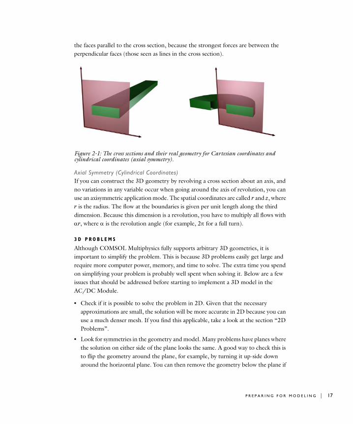
the faces parallel to the cross section, because the strongest forces are between the perpendicular faces (those seen as lines in the cross section).
Figure 2-1: The cross sections and their real geometry for Cartesian coordinates and cylindrical coordinates (axial symmetry).
Axial Symmetry (Cylindrical Coordinates)If you can construct the 3D geometry by revolving a cross section about an axis, and no variations in any variable occur when going around the axis of revolution, you can use an axisymmetric application mode. The spatial coordinates are called r and z, where r is the radius. The flow at the boundaries is given per unit length along the third dimension. Because this dimension is a revolution, you have to multiply all flows with αr, where α is the revolution angle (for example, 2π for a full turn).
3 D P R O B L E M S
Although COMSOL Multiphysics fully supports arbitrary 3D geometries, it is important to simplify the problem. This is because 3D problems easily get large and require more computer power, memory, and time to solve. The extra time you spend on simplifying your problem is probably well spent when solving it. Below are a few issues that should be addressed before starting to implement a 3D model in the AC/DC Module.
• Check if it is possible to solve the problem in 2D. Given that the necessary approximations are small, the solution will be more accurate in 2D because you can use a much denser mesh. If you find this applicable, take a look at the section “2D Problems”.
• Look for symmetries in the geometry and model. Many problems have planes where the solution on either side of the plane looks the same. A good way to check this is to flip the geometry around the plane, for example, by turning it up-side down around the horizontal plane. You can then remove the geometry below the plane if
P R E P A R I N G F O R M O D E L I N G | 17
18 | C H A P T E R
you do not see any differences between the two cases regarding geometry, materials, and sources. Boundaries created by the cross section between the geometry and this plane need a symmetry boundary condition, which is available in all 3D application modes. See “Eddy Currents in 3D” on page 202 in the AC/DC Module Model Library for an example.
• There are also cases when the dependence along one direction is known, so you can replace it by an analytical function. You can use this approach either to convert 3D to 2D or to convert a layer to a boundary condition (see also the section “Boundary Conditions”).
B O U N D A R Y C O N D I T I O N S
An important technique to minimize the problem size is to use efficient boundary conditions. Truncating the geometry without introducing too large errors is one of the great challenges in modeling. Below are a few suggestions of how to do this. They apply to both 2D and 3D problems.
• Many models extend to infinity or might have regions where the solution only undergoes small changes. This problem is addressed in two related steps. First, you need to truncate the geometry in a suitable position. Second, you need to apply a suitable boundary condition there. For static and quasi-static models, it is often possible to assume zero fields at the open boundary, provided that this is at a sufficient distance away from the sources.
• Replace thin layers with boundary conditions where possible. There are several types of boundary conditions in COMSOL Multiphysics suitable for such replacements. You can, for example, replace materials with high conductivity with the shielding boundary condition, which assumes a constant potential through the thickness of the layer. If you have a magnetic material with a high relative permeability, you can also model it using the shielding boundary condition (see the model “Magnetic Signature of a Submarine” on page 241 in the AC/DC Module Model Library).
• Use boundary conditions for known solutions. A current-carrying wire with a high conductivity at high frequency has the current density confined to a thin region beneath the surface of the wire. If it is possible to calculate the total current, you can often replace the current in the wire by a surface current boundary condition (see “Inductive Heating of a Copper Cylinder” on page 16 in the AC/DC Module Model Library).
2 : A C / D C M O D E L I N G
S O U R C E S
You can apply electromagnetic sources in many different ways. The typical options are volume sources, boundary sources, line sources, and point sources, where point sources in 2D formulations are equivalent to line sources in 3D formulations. The way sources are imposed can have an impact on what quantities you can compute from the model. For example, a point source in an electrostatics model represents a singularity, and the electric potential does not have a finite value at the position of the source. In a COMSOL Multiphysics model, a point source has a finite but mesh-dependent value. Thus, it does not make sense to compute a point-to-point capacitance, because this is defined as the ratio of charge to voltage. In general, using volume or boundary sources is more flexible than using line or point sources but the meshing of the source domains becomes more expensive.
Meshing and Solving
The finite element method approximates the solution within each element, using some elementary shape function that can be constant, linear, or of higher order. Depending on the element order in the model, a finer or coarser mesh is required to resolve the solution. In general, there are three problem-dependent factors that determine the necessary mesh resolution:
• The first is the variation in the solution due to geometrical factors. The mesh generator automatically generates a finer mesh where there is a lot of fine geometrical details. Try to remove such details if they do not influence the solution, because they produce a lot of unnecessary mesh elements.
• The second is the skin effect or the field variation due to losses. It is easy to estimate the skin depth from the conductivity, permeability, and frequency. You need at least two linear elements per skin depth to capture the variation of the fields. If you do not study the skin depth, you can replace regions with a small skin depth with a boundary condition, thereby saving elements.
• The third and last factor is the wavelength. To resolve a wave properly, it is necessary to use about 10 linear (or 5 2nd-order) elements per wavelength. Keep in mind that the wavelength might be shorter in a dielectric medium.
S O L V E R S
You can, in most cases, use the solver that COMSOL Multiphysics suggests. The choice of solver is optimized for the typical case for each application mode and analysis type in the AC/DC Module. However, in special cases you might need to tune the solver settings. This is especially important for 3D problems, because they use a large
P R E P A R I N G F O R M O D E L I N G | 19

20 | C H A P T E R
amount of memory. For extremely large 3D problems, you may need a 64-bit platform. You can find a more detailed description on the solver settings in “Solving the Model” on page 359 in the COMSOL Multiphysics User’s Guide. See also “Solving Large 3D Problems” on page 84.
2 : A C / D C M O D E L I N G
An Examp l e—Eddy Cu r r e n t s
Introduction
To help you understand how to create models using the AC/DC Module, this section walks through an example in great detail. You can apply these techniques to all the models in this module, other optional modules, or even the many models that ship with the base COMSOL Multiphysics package.
The first example model concerns an AC coil surrounding a metal cylinder, and the coil induces eddy currents in the cylinder. It illustrates how to examine a system using several different approaches. You can model the coil with or without the skin effect, and it shows how varying the frequency of the current source also alters the depth of the skin effect.
Model Definition
To build this model, work with the axisymmetric Quasi-Statics Azimuthal Currents application mode and a time-harmonic formulation. The model represents the cylinder as a rectangle and the coil as a circle. The modeling plane is the rz-plane; the horizontal axis represents the r-axis, and the vertical axis represents the z-axis. To obtain the actual 3D geometry, revolve the 2D geometry about the z-axis.
D O M A I N E Q U A T I O N S
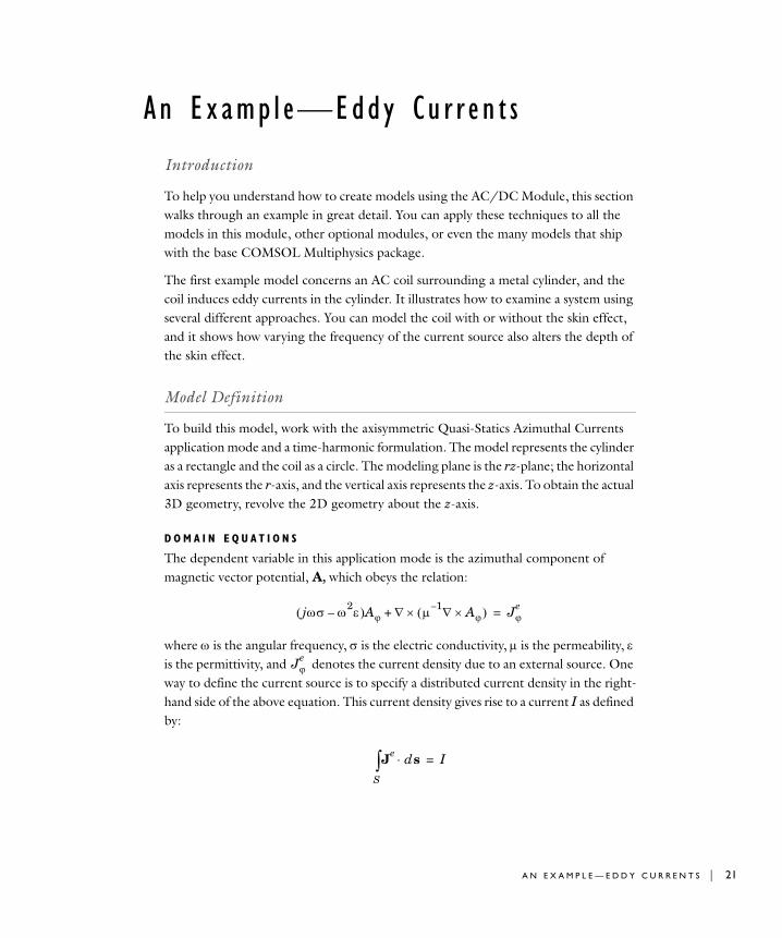
The dependent variable in this application mode is the azimuthal component of magnetic vector potential, A, which obeys the relation:
where ω is the angular frequency, σ is the electric conductivity, µ is the permeability, ε is the permittivity, and denotes the current density due to an external source. One way to define the current source is to specify a distributed current density in the right-hand side of the above equation. This current density gives rise to a current I as defined by:
jωσ ω2ε–( )Aϕ ∇ µ 1– ∇ Aϕ×( )×+ Jϕe
=
Jϕe
Je ds⋅S∫ I=
A N E X A M P L E — E D D Y C U R R E N T S | 21
22 | C H A P T E R
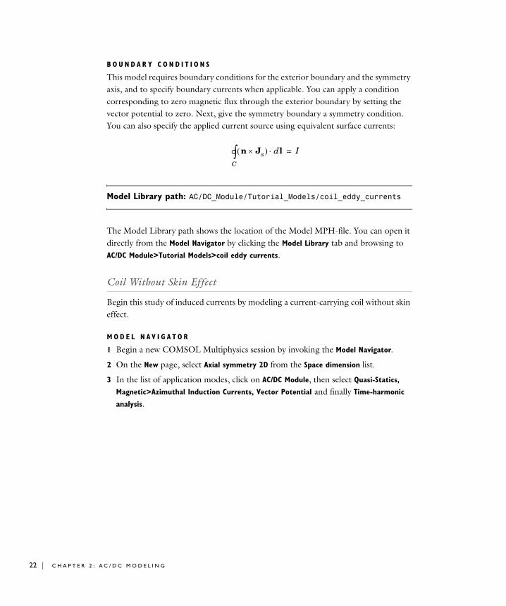
B O U N D A R Y C O N D I T I O N S
This model requires boundary conditions for the exterior boundary and the symmetry axis, and to specify boundary currents when applicable. You can apply a condition corresponding to zero magnetic flux through the exterior boundary by setting the vector potential to zero. Next, give the symmetry boundary a symmetry condition. You can also specify the applied current source using equivalent surface currents:
Model Library path: AC/DC_Module/Tutorial_Models/coil_eddy_currents
The Model Library path shows the location of the Model MPH-file. You can open it directly from the Model Navigator by clicking the Model Library tab and browsing to AC/DC Module>Tutorial Models>coil eddy currents.
Coil Without Skin Effect
Begin this study of induced currents by modeling a current-carrying coil without skin effect.
M O D E L N A V I G A T O R
1 Begin a new COMSOL Multiphysics session by invoking the Model Navigator.
2 On the New page, select Axial symmetry 2D from the Space dimension list.
3 In the list of application modes, click on AC/DC Module, then select Quasi-Statics,
Magnetic>Azimuthal Induction Currents, Vector Potential and finally Time-harmonic
analysis.
n Js×( ) dl⋅C∫° I=
2 : A C / D C M O D E L I N G
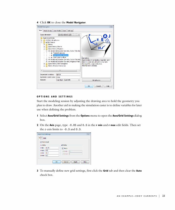
4 Click OK to close the Model Navigator.
O P T I O N S A N D S E T T I N G S
Start the modeling session by adjusting the drawing area to hold the geometry you plan to draw. Another aid in making the simulation easier is to define variables for later use when defining the problem.
1 Select Axes/Grid Settings from the Options menu to open the Axes/Grid Settings dialog box.
2 On the Axis page, type -0.05 and 0.5 in the r min and r max edit fields. Then set the z-axis limits to -0.3 and 0.3.
3 To manually define new grid settings, first click the Grid tab and then clear the Auto check box.
A N E X A M P L E — E D D Y C U R R E N T S | 23
24 | C H A P T E R
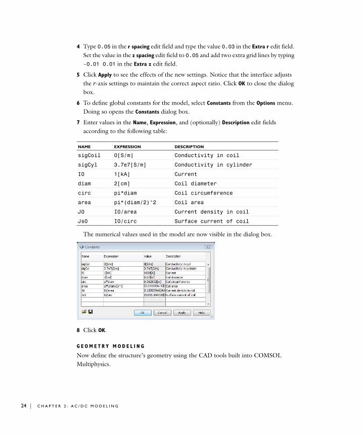
4 Type 0.05 in the r spacing edit field and type the value 0.03 in the Extra r edit field. Set the value in the z spacing edit field to 0.05 and add two extra grid lines by typing -0.01 0.01 in the Extra z edit field.
5 Click Apply to see the effects of the new settings. Notice that the interface adjusts the r-axis settings to maintain the correct aspect ratio. Click OK to close the dialog box.
6 To define global constants for the model, select Constants from the Options menu. Doing so opens the Constants dialog box.
7 Enter values in the Name, Expression, and (optionally) Description edit fields according to the following table:
The numerical values used in the model are now visible in the dialog box.
8 Click OK.
G E O M E T R Y M O D E L I N G
Now define the structure’s geometry using the CAD tools built into COMSOL Multiphysics.
NAME EXPRESSION DESCRIPTION
sigCoil 0[S/m] Conductivity in coil
sigCyl 3.7e7[S/m] Conductivity in cylinder
I0 1[kA] Current
diam 2[cm] Coil diameter
circ pi*diam Coil circumference
area pi*(diam/2)^2 Coil area
J0 I0/area Current density in coil
Js0 I0/circ Surface current of coil
2 : A C / D C M O D E L I N G
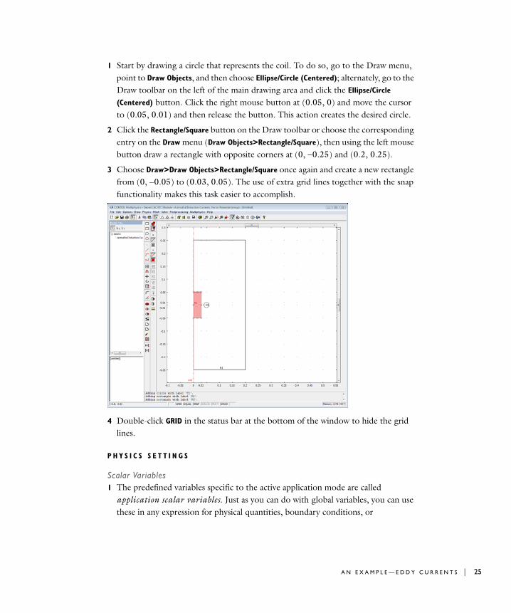
1 Start by drawing a circle that represents the coil. To do so, go to the Draw menu, point to Draw Objects, and then choose Ellipse/Circle (Centered); alternately, go to the Draw toolbar on the left of the main drawing area and click the Ellipse/Circle
(Centered) button. Click the right mouse button at (0.05, 0) and move the cursor to (0.05, 0.01) and then release the button. This action creates the desired circle.
2 Click the Rectangle/Square button on the Draw toolbar or choose the corresponding entry on the Draw menu (Draw Objects>Rectangle/Square), then using the left mouse button draw a rectangle with opposite corners at (0, −0.25) and (0.2, 0.25).
3 Choose Draw>Draw Objects>Rectangle/Square once again and create a new rectangle from (0, −0.05) to (0.03, 0.05). The use of extra grid lines together with the snap functionality makes this task easier to accomplish.
4 Double-click GRID in the status bar at the bottom of the window to hide the grid lines.
P H Y S I C S S E T T I N G S
Scalar Variables1 The predefined variables specific to the active application mode are called
application scalar variables. Just as you can do with global variables, you can use these in any expression for physical quantities, boundary conditions, or
A N E X A M P L E — E D D Y C U R R E N T S | 25
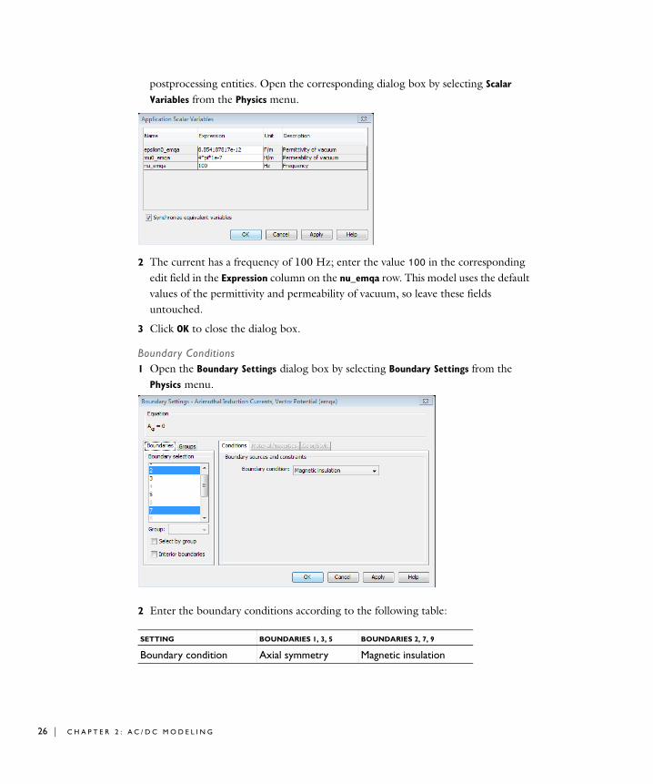
26 | C H A P T E R
postprocessing entities. Open the corresponding dialog box by selecting Scalar Variables from the Physics menu.
2 The current has a frequency of 100 Hz; enter the value 100 in the corresponding edit field in the Expression column on the nu_emqa row. This model uses the default values of the permittivity and permeability of vacuum, so leave these fields untouched.
3 Click OK to close the dialog box.
Boundary Conditions1 Open the Boundary Settings dialog box by selecting Boundary Settings from the
Physics menu.
2 Enter the boundary conditions according to the following table:
SETTING BOUNDARIES 1, 3, 5 BOUNDARIES 2, 7, 9
Boundary condition Axial symmetry Magnetic insulation
2 : A C / D C M O D E L I N G
Note: You can select a boundary either in the Boundary selection list or by clicking on it in the main drawing area. To select several boundaries simultaneously, use the Shift and Ctrl keys.
3 Click OK.
Boundaries 1, 3, and 5 make up the vertical boundary along the z-axis, and the axial symmetry boundary condition makes certain the solution is symmetric around this axis. The boundary condition at the other three boundaries (2, 7, and 9) sets the magnetic potential, , to zero along that boundary.
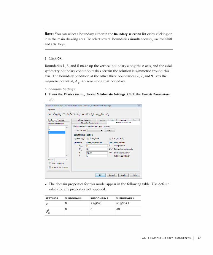
Subdomain Settings1 From the Physics menu, choose Subdomain Settings. Click the Electric Parameters
tab.
2 The domain properties for this model appear in the following table. Use default values for any properties not supplied.
SETTINGS SUBDOMAIN 1 SUBDOMAIN 2 SUBDOMAIN 3
σ 0 sigCyl sigCoil
0 0 J0
Aϕ
Jϕe
A N E X A M P L E — E D D Y C U R R E N T S | 27
28 | C H A P T E R
3 Click OK.
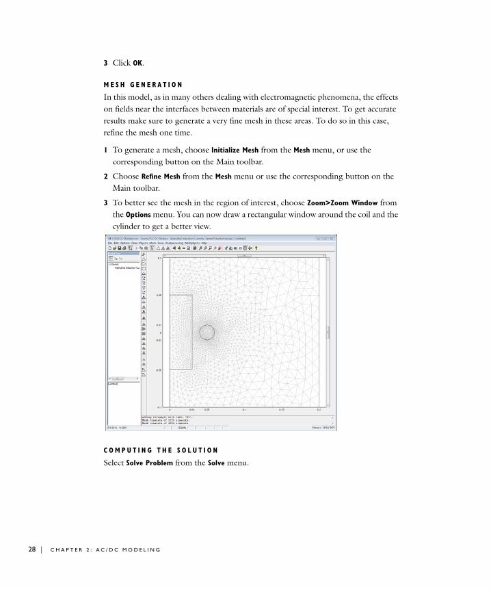
M E S H G E N E R A T I O N
In this model, as in many others dealing with electromagnetic phenomena, the effects on fields near the interfaces between materials are of special interest. To get accurate results make sure to generate a very fine mesh in these areas. To do so in this case, refine the mesh one time.
1 To generate a mesh, choose Initialize Mesh from the Mesh menu, or use the corresponding button on the Main toolbar.
2 Choose Refine Mesh from the Mesh menu or use the corresponding button on the Main toolbar.
3 To better see the mesh in the region of interest, choose Zoom>Zoom Window from the Options menu. You can now draw a rectangular window around the coil and the cylinder to get a better view.
C O M P U T I N G T H E S O L U T I O N
Select Solve Problem from the Solve menu.
2 : A C / D C M O D E L I N G
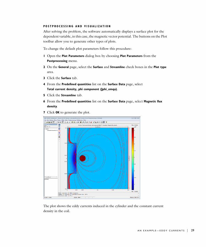
PO S T P R O C E S S I N G A N D V I S U A L I Z A T I O N
After solving the problem, the software automatically displays a surface plot for the dependent variable, in this case, the magnetic vector potential. The buttons on the Plot toolbar allow you to generate other types of plots.
To change the default plot parameters follow this procedure:
1 Open the Plot Parameters dialog box by choosing Plot Parameters from the Postprocessing menu.
2 On the General page, select the Surface and Streamline check boxes in the Plot type area.
3 Click the Surface tab.
4 From the Predefined quantities list on the Surface Data page, select Total current density, phi component (Jphi_emqa).
5 Click the Streamline tab.
6 From the Predefined quantities list on the Surface Data page, select Magnetic flux
density.
7 Click OK to generate the plot.
The plot shows the eddy currents induced in the cylinder and the constant current density in the coil.
A N E X A M P L E — E D D Y C U R R E N T S | 29
30 | C H A P T E R
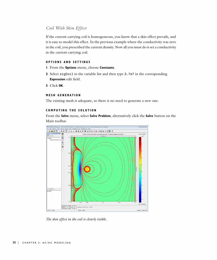
Coil With Skin Effect
If the current-carrying coil is homogeneous, you know that a skin effect prevails, and it is easy to model this effect. In the previous example where the conductivity was zero in the coil, you prescribed the current density. Now all you must do is set a conductivity in the current-carrying coil.
O P T I O N S A N D S E T T I N G S
1 From the Options menu, choose Constants.
2 Select sigCoil in the variable list and then type 3.7e7 in the corresponding Expression edit field.
3 Click OK.
M E S H G E N E R A T I O N
The existing mesh is adequate, so there is no need to generate a new one.
C O M P U T I N G T H E S O L U T I O N
From the Solve menu, select Solve Problem; alternatively click the Solve button on the Main toolbar.
The skin effect in the coil is clearly visible.
2 : A C / D C M O D E L I N G
The Use of Surface Currents
You can also create a similar model by specifying surface currents at the coil’s boundaries. To do so you must modify the boundary conditions around the coil and remove the current source inside the domain representing the coil.
O P T I O N S A N D S E T T I N G S
Because you can consider all currents as concentrated at the coil boundaries, set the conductivity in the coil domain to zero. Otherwise the surface currents would induce currents in the interior of the domain in the opposite direction.
1 From the Options menu, open the Constants dialog box.
2 Set the Expression of the variable sigCoil to 0, then click OK.
P H Y S I C S S E T T I N G S
Boundary Conditions1 From the Physics menu, choose Boundary Settings to open the Boundary Settings
dialog box.
2 Select the Interior Boundaries check box.
3 Do not change the boundary conditions at the exterior boundaries of the domain, but set the conditions at the interior boundaries according to the following table:
Subdomain Settings1 Open the Subdomain Settings dialog box.
2 Do not alter the properties in the cylinder and the surrounding air, but modify the parameters in the coil as follows:
M E S H G E N E R A T I O N
The existing mesh is adequate so there is no need to generate a new one.
SETTINGS BOUNDARIES 10–13
Boundary condition Surface current
Js0
SETTINGS SUBDOMAIN 3
σ sigCoil
0
Jsϕ
Jϕe
A N E X A M P L E — E D D Y C U R R E N T S | 31
32 | C H A P T E R
C O M P U T I N G T H E S O L U T I O N
From the Solve menu, select Solve Problem or click the Solve button on the Main toolbar.
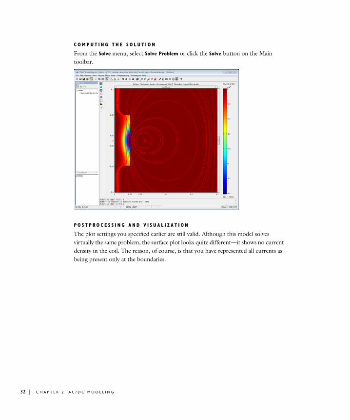
PO S T P R O C E S S I N G A N D V I S U A L I Z A T I O N
The plot settings you specified earlier are still valid. Although this model solves virtually the same problem, the surface plot looks quite different—it shows no current density in the coil. The reason, of course, is that you have represented all currents as being present only at the boundaries.
2 : A C / D C M O D E L I N G
F l o a t i n g Po t e n t i a l s a nd E l e c t r i c S h i e l d i n g
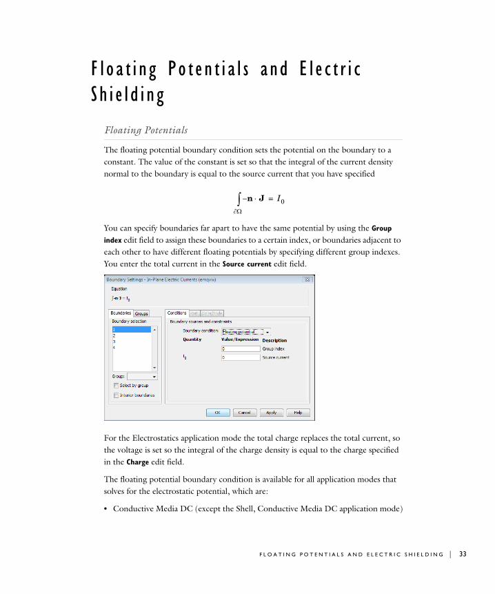
Floating Potentials
The floating potential boundary condition sets the potential on the boundary to a constant. The value of the constant is set so that the integral of the current density normal to the boundary is equal to the source current that you have specified
You can specify boundaries far apart to have the same potential by using the Group
index edit field to assign these boundaries to a certain index, or boundaries adjacent to each other to have different floating potentials by specifying different group indexes. You enter the total current in the Source current edit field.
For the Electrostatics application mode the total charge replaces the total current, so the voltage is set so the integral of the charge density is equal to the charge specified in the Charge edit field.
The floating potential boundary condition is available for all application modes that solves for the electrostatic potential, which are:
• Conductive Media DC (except the Shell, Conductive Media DC application mode)
n– J⋅Ω∂∫ I0=
F L O A T I N G P O T E N T I A L S A N D E L E C T R I C S H I E L D I N G | 33
34 | C H A P T E R
• Electrostatics
• Quasi-Statics, Electric—Electric Currents
• Quasi-Statics, Electromagnetic—Electric and Induction Currents
It is also available for all analysis types. For the Quasi-Statics, Electromagnetic application mode, which solves for both the electrostatic potential and the magnetic vector potential, it is necessary to select a constraint boundary condition on the vector potential for the floating potential condition to become available. The constraint boundary conditions are Magnetic insulation and Magnetic potential, and you find them on the Magnetic Parameters page. Any other condition disables the Electric Parameter page, which holds all the electric boundary conditions. It is on this page you can select the floating potential boundary condition.
Electric Shielding
The electric shielding condition adds the same equation as in the subdomain on the boundary using tangential derivative variables. You can read more about these variables in the section “Modeling with PDEs on Boundaries, Edges, and Points” on page 294 in the COMSOL Multiphysics Modeling Guide. This is the equation used for the Conductive Media DC application mode.
The variable d accounts for the thickness of the shield, but the solution is constant through the thickness. The conductivity that you enter here is the conductivity of the boundary. You can use this boundary condition when approximating a thin subdomain with a boundary to reduce the number of mesh elements.
∇t σd Vt∇( )⋅– 0=
2 : A C / D C M O D E L I N G
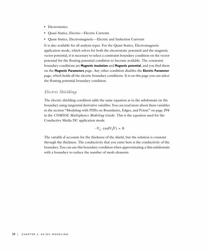
For the Quasi-statics, Electric application mode, it is also possible to specify a dielectric constant.
The Electrostatics application mode only uses the relative permittivity material parameter. In addition, you can specify a surface charge density.
Example Model—Floating Potential
This is a tutorial model to show how to use the floating potential and electric shielding boundary conditions in the Conductive Media DC application mode. The analysis includes solving the same model changing between the two different boundary conditions and with and without weak constraints on the boundaries.
Model Definition
The modeling domain is a box filled with air containing an electrode. The sides of the box are insulated while the top has a potential and the bottom is grounded.
B O U N D A R Y C O N D I T I O N S O N T H E E L E C T R O D E
First use the electric shielding boundary condition on the electrode. Setting the conductivity of the electrode to the conductivity of a metal gives you an electrode with an almost constant potential. In this way you can set a constant potential without knowing the actual value of it.
F L O A T I N G P O T E N T I A L S A N D E L E C T R I C S H I E L D I N G | 35
36 | C H A P T E R
Then set the boundary condition on the electrode to a floating potential. If the source current is zero this gives you a potential so that the flux over the boundary is zero. The integral is calculated with a coupling variable. You can keep the default solver settings.
Finally solve the model with a floating potential boundary condition and use weak constraints on the electrode. The reason to use the weak constraints is that this gives a more accurate computation of the current density normal to the boundary in the postprocessing stage. When using weak constraints you solve for the variable lm1 (the Lagrange multiplier), which is equal to the normal flux on the boundary. The floating point boundary condition uses this variable to calculate the integral of the current flowing to the boundary. You cannot use the default AMG preconditioner when dealing with weak constraints, so therefore you need to select the Incomplete LU preconditioner instead. Note that the solution is exactly the same with and without weak constraints, it is access to the accurate flux that you get with weak constraints. For more information on weak constraints, see “Using Weak Constraints” on page 300 in the COMSOL Multiphysics Modeling Guide.
Results and Discussion
The differences between the three ways to model a floating electrode can be investigated by calculating the integral of the current flowing to the electrode. Ideally, this current should be zero. Using the electric shielding boundary condition, you get a current of approximately 0.19 A. Using the floating potential boundary condition without weak constraints, you also get a current of 0.19 A, most of which is due to interpolation errors. Finally, when using weak constraints, you get a current of about 8.9 nA. The approach using weak constraints is clearly the best if you need access to the total flux. The electric shielding boundary condition does not strictly impose a fixed potential on the electrode as it allows for a small but finite tangential gradient in the potential which of course may be an advantage if you need to account for small resistive loss in the electrode. The advantage of not using weak constraints is that you can use the default solver settings.
Model Library path: ACDC_Module/Tutorial_Models/floating_potential
2 : A C / D C M O D E L I N G
Modeling Using the Graphical User Interface
M O D E L N A V I G A T O R
1 In the Model Navigator select 3D from the Space dimension list.
2 Open the AC/DC Module folder, then select Statics>Conductive Media DC.
3 Click OK.
G E O M E T R Y M O D E L I N G
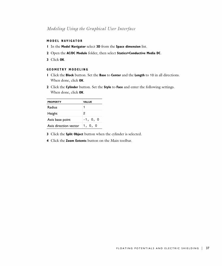
1 Click the Block button. Set the Base to Center and the Length to 10 in all directions. When done, click OK.
2 Click the Cylinder button. Set the Style to Face and enter the following settings. When done, click OK.
3 Click the Split Object button when the cylinder is selected.
4 Click the Zoom Extents button on the Main toolbar.
PROPERTY VALUE
Radius 1
Height 2
Axis base point -1, 0, 0
Axis direction vector 1, 0, 0
F L O A T I N G P O T E N T I A L S A N D E L E C T R I C S H I E L D I N G | 37
38 | C H A P T E R
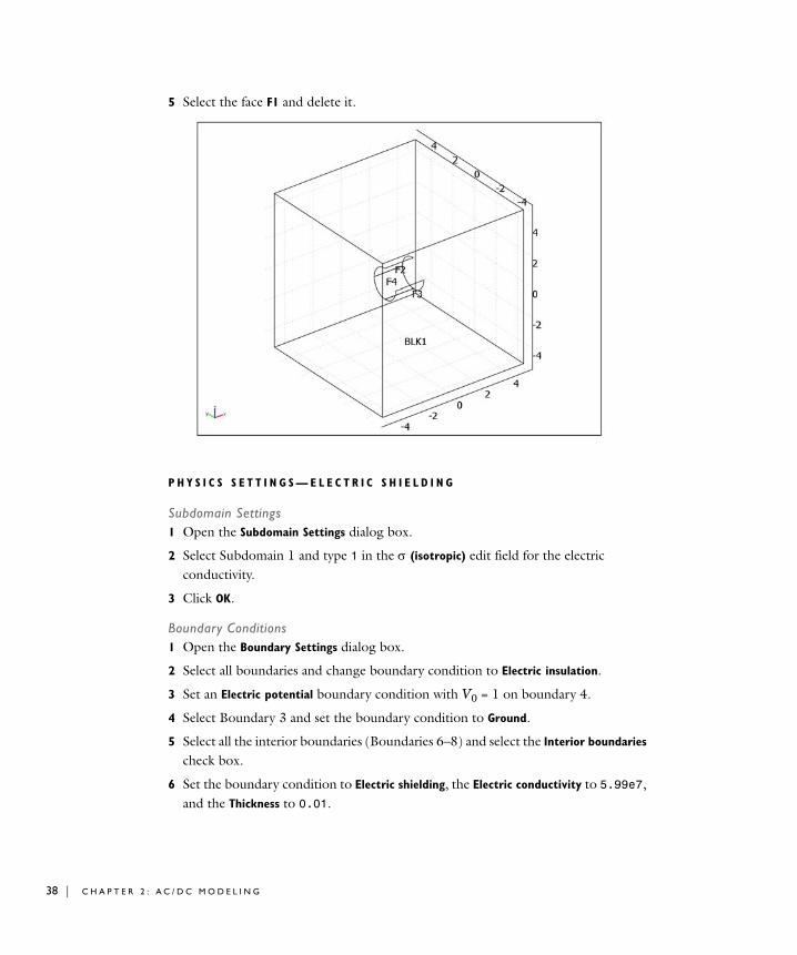
5 Select the face F1 and delete it.
P H Y S I C S S E T T I N G S — E L E C T R I C S H I E L D I N G
Subdomain Settings1 Open the Subdomain Settings dialog box.
2 Select Subdomain 1 and type 1 in the σ (isotropic) edit field for the electric conductivity.
3 Click OK.
Boundary Conditions1 Open the Boundary Settings dialog box.
2 Select all boundaries and change boundary condition to Electric insulation.
3 Set an Electric potential boundary condition with V0 = 1 on boundary 4.
4 Select Boundary 3 and set the boundary condition to Ground.
5 Select all the interior boundaries (Boundaries 6–8) and select the Interior boundaries check box.
6 Set the boundary condition to Electric shielding, the Electric conductivity to 5.99e7, and the Thickness to 0.01.
2 : A C / D C M O D E L I N G
7 Click OK.
M E S H G E N E R A T I O N A N D S O L U T I O N
Initialize the mesh and solve with the default settings.
PO S T P R O C E S S I N G A N D V I S U A L I Z A T I O N
Calculate the integral of the current flowing to the electrode.
1 Open the Boundary Integration dialog box from the Postprocessing menu.
2 Type nJs_emdc in the Expression field and click Apply.
The result appears in the message log at the bottom of the user interface. The current is approximately 0.19 A.
P H Y S I C S S E T T I N G S — F L O A T I N G PO T E N T I A L
Boundary Conditions1 Open the Boundary Settings dialog box.
2 Select Boundaries 6–8.
3 Set the boundary condition to Floating potential.
4 Click OK.
M E S H G E N E R A T I O N A N D S O L U T I O N
Initialize the mesh and solve with the default settings.
PO S T P R O C E S S I N G A N D V I S U A L I Z A T I O N
Calculate the integral of the current flowing to the electrode.
1 Open the Boundary Integration dialog box from the Postprocessing menu.
2 Type nJs_emdc in the Expression field and click Apply.
The result appears in the message log at the bottom of the user interface. You should get a current of approximately 0.19 A. Note that this current calculation is not very accurate; the actual current is almost zero. It is the evaluation of the derivatives in the expression for nJs_emdc that is the source of the error.
P R O P E R T I E S — WE A K C O N S T R A I N T S
1 From the Physics menu, choose Properties to open the Application Model Properties dialog box.
2 Select On from the Weak constraints list, then click OK.
F L O A T I N G P O T E N T I A L S A N D E L E C T R I C S H I E L D I N G | 39
40 | C H A P T E R
P H Y S I C S S E T T I N G S — WE A K C O N S T R A I N T S
Boundary Conditions1 Open the Boundary Settings dialog box.
2 Select Boundaries 6–8.
3 Click the Weak Constr. tab and make sure that Use weak constraints is selected.
4 Click OK.
M E S H G E N E R A T I O N
Click the Initialize Mesh button on the Main toolbar.
C O M P U T I N G T H E S O L U T I O N
1 Open the Solver Parameters dialog box.
2 Change the Linear system solver to GMRES.
3 Make sure that Automatic or Nonsymmetric is selected in the Matrix symmetry list.
4 Change the Preconditioner to Incomplete LU.
5 Click OK.
6 Click the Solve button on the Main toolbar to compute the solution.
If you selected Automatic in the Matrix symmetry list, a warning message appears. You can ignore this warning because it only tells you that the solver settings cannot take advantage of the matrix symmetry, so the solver uses the nonsymmetric setting instead.
PO S T P R O C E S S I N G A N D V I S U A L I Z A T I O N
Calculate the integral of the current flowing to the electrode.
1 Open the Boundary Integration dialog box from the Postprocessing menu.
2 Select Boundaries 6–8.
3 Type nJs_emdc in the Expression field, then click OK.
The result appears in the message log at the bottom of the user interface. You should get a current of approximately 8.9·10−9 A. This is also the true value of the total current in the previous solution step without weak constraints.
To plot the potential on the electrode as a boundary plot, suppress the display of some of the outer boundaries:
1 In the Options menu, select Suppress>Suppress Boundaries.
2 Select Boundaries 6–8, then click Apply.
2 : A C / D C M O D E L I N G
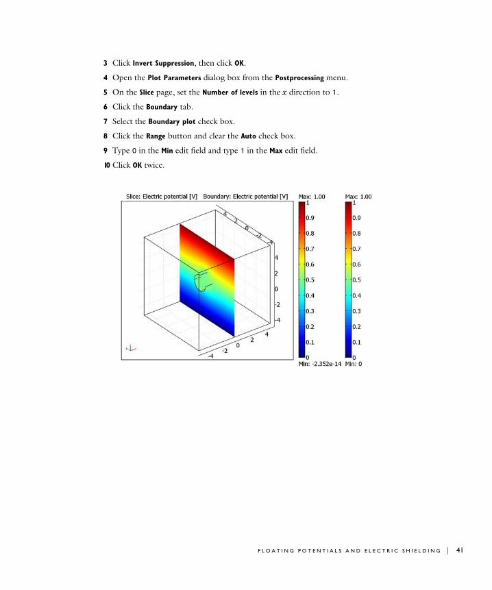
3 Click Invert Suppression, then click OK.
4 Open the Plot Parameters dialog box from the Postprocessing menu.
5 On the Slice page, set the Number of levels in the x direction to 1.
6 Click the Boundary tab.
7 Select the Boundary plot check box.
8 Click the Range button and clear the Auto check box.
9 Type 0 in the Min edit field and type 1 in the Max edit field.
10 Click OK twice.
F L O A T I N G P O T E N T I A L S A N D E L E C T R I C S H I E L D I N G | 41
42 | C H A P T E R
Pe r i o d i c Bounda r y Cond i t i o n s
The section “Using Periodic Boundary Conditions” on page 245 in the COMSOL Multiphysics User’s Guide presents a general description on how to define periodic Boundary conditions. The AC/DC Module has an automatic Periodic condition accessible from the Boundary Settings dialog box, so it is not necessary to use the Periodic Boundary Conditions dialog box. Use the latter dialog box for special cases when you need full control of the periodic condition. The automatic periodic condition can identify simple mappings on plane groups of source and destination boundaries with equal shape. The destination can also be rotated with respect to the source.
The application modes that use vector elements include a variable, Ψ, that implements an extra equation to explicitly set the divergence of the A field to zero. Similar to using assemblies with vector elements, periodic conditions must use this extra equation when the source and destination of the periodic condition have incompatible meshes; see “Using Assemblies in Electromagnetics Problems” on page 97 for more details. This variable Ψ must also be made periodic, something the automatic periodic condition takes care of if the Gauge fixing is turned on or is set to automatic. You must explicitly turn the Gauge fixing off if you use an application mode that does not require Gauge fixing and you have compatible meshes for the periodic boundaries. The following list shows the application modes that use vector elements:
• Magnetostatics for 3D, in-plane currents or meridional currents.
• Quasi-statics, Magnetic for 3D, in-plane or meridional currents.
• Quasi-statics, Electromagnetic for 3D, in-plane or meridional currents.
All other application modes do not need any special consideration when using periodic boundaries.
User Interface for Periodic Conditions
You specify the periodic condition in the Physics>Boundary Settings dialog box. Select the boundaries that define one periodic condition and choose Periodic condition from the Boundary condition list. The boundaries can consist of one or more source boundaries plus one or more destination boundaries. The combined cross section of all source boundaries must be equal in shape to the combined cross section of all destination boundaries. If you want several periodic conditions with different
2 : A C / D C M O D E L I N G
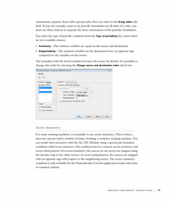
orientations, separate them with a group index that you enter in the Group index edit field. If you, for example, want to set periodic boundaries on all sides of a cube, you must use three indexes to separate the three orientations of the periodic boundaries.
You select the type of periodic condition from the Type of periodicity list, where there are two available choices:
• Continuity—The solution variables are equal on the source and destination.
• Antiperiodicity—The solution variables on the destination have an opposite sign compared to the variables on the source.
The boundary with the lowest number becomes the source by default. It is possible to change this order by selecting the Change source and destination order check box.
Sector Symmetry
For many rotating machines, it is possible to use sector symmetry. This is when a structure repeats itself a number of times, forming a complete rotating machine. You can model such structures with the AC/DC Module using a special pair boundary condition called sector symmetry. The condition has two versions: sector symmetry and sector antisymmetry. For sector symmetry, the sources in one sector are mapped using the identity map to the other sectors. In sector antisymmetry, the sources are mapped with an opposite sign with respect to the neighboring sector. The sector symmetry condition is only available for the Perpendicular Currents application mode with static or transient analysis.
P E R I O D I C B O U N D A R Y C O N D I T I O N S | 43
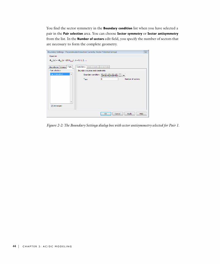
44 | C H A P T E R
You find the sector symmetry in the Boundary condition list when you have selected a pair in the Pair selection area. You can choose Sector symmetry or Sector antisymmetry from the list. In the Number of sectors edit field, you specify the number of sectors that are necessary to form the complete geometry.
Figure 2-2: The Boundary Settings dialog box with sector antisymmetry selected for Pair 1.
2 : A C / D C M O D E L I N G
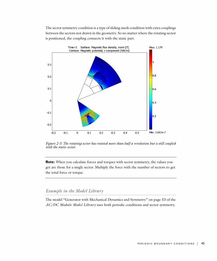
The sector symmetry condition is a type of sliding mesh condition with extra couplings between the sectors not drawn in the geometry. So no matter where the rotating sector is positioned, the coupling connects it with the static part.
Figure 2-3: The rotating sector has rotated more than half a revolution but is still coupled with the static sector.
Note: When you calculate forces and torques with sector symmetry, the values you get are those for a single sector. Multiply the force with the number of sectors to get the total force or torque.
Example in the Model Library
The model “Generator with Mechanical Dynamics and Symmetry” on page 53 of the AC/DC Module Model Library uses both periodic conditions and sector symmetry.
P E R I O D I C B O U N D A R Y C O N D I T I O N S | 45
46 | C H A P T E R
I n f i n i t e E l emen t s
Many environments that are modeled with finite elements are unbounded or open, meaning that the electromagnetic fields extend toward infinity. The easiest approach to modeling an unbounded domain is to extend the simulation domain “far enough” that the influence of the terminating boundary conditions at the far end becomes negligible. This approach can create unnecessary mesh elements and make the geometry difficult to mesh due to large differences between the largest and smallest object.
Another approach is to use infinite elements. There are many implementations of infinite elements available, and the one used in the AC/DC Module is often referred to as mapped infinite elements (see Ref. ?). This implementation maps the model coordinates from the local, finite-sized domain, to a stretched domain. The inner boundary of this stretched domain is coincident with the local domain, but at the exterior boundary the coordinates are scaled toward infinity.
The inner coordinate, t0, and the width of the infinite element region, δ t, are input parameters for each region. The software uses default values for these properties for geometries that are Cartesian, cylindrical, or spherical. However, these default parameters might not work well for complex geometries, so it might be necessary to define other parameters. The following figures show typical examples of infinite element regions that work nicely for each of the infinite element types. These types are:
• Stretching in Cartesian coordinate directions, labeled Cartesian.
• Stretching in cylindrical directions, labeled Cylindrical.
• Stretching in spherical direction, labeled Spherical.
• User-defined coordinate transform for general infinite elements.
t' t0δt
t0 δt t–+------------------------=
2 : A C / D C M O D E L I N G
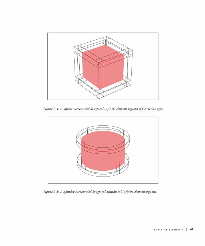
Figure 2-4: A square surrounded by typical infinite-element regions of Cartesian type.
Figure 2-5: A cylinder surrounded by typical cylindrical infinite-element regions.
I N F I N I T E E L E M E N T S | 47
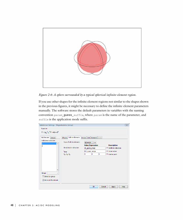
48 | C H A P T E R
Figure 2-6: A sphere surrounded by a typical spherical infinite-element region.
If you use other shapes for the infinite element regions not similar to the shapes shown in the previous figures, it might be necessary to define the infinite-element parameters manually. The software stores the default parameters in variables with the naming convention param_guess_suffix, where param is the name of the parameter, and suffix is the application mode suffix.
2 : A C / D C M O D E L I N G
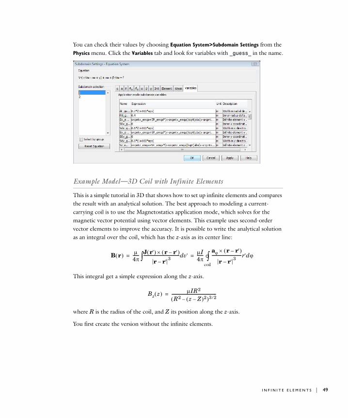
You can check their values by choosing Equation System>Subdomain Settings from the Physics menu. Click the Variables tab and look for variables with _guess_ in the name.
Example Model—3D Coil with Infinite Elements
This is a simple tutorial in 3D that shows how to set up infinite elements and compares the result with an analytical solution. The best approach to modeling a current-carrying coil is to use the Magnetostatics application mode, which solves for the magnetic vector potential using vector elements. This example uses second-order vector elements to improve the accuracy. It is possible to write the analytical solution as an integral over the coil, which has the z-axis as its center line:
This integral get a simple expression along the z-axis.
where R is the radius of the coil, and Z its position along the z-axis.
You first create the version without the infinite elements.
B r( ) µ4π------ J r'( ) r r'–( )×
r r'–3
------------------------------------- v'd∫ µI4π------
aϕ r r'–( )×
r r'–3
-------------------------------r'dϕcoil∫°= =
Bz z( ) µIR2
R2 z Z–( )2–( )3 2/----------------------------------------------=
I N F I N I T E E L E M E N T S | 49
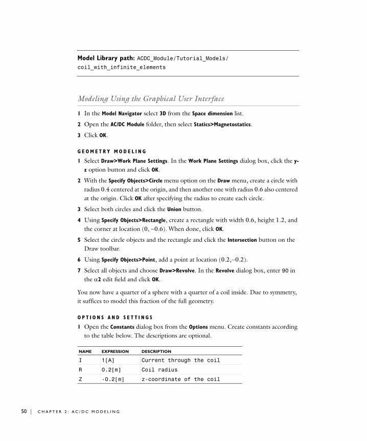
50 | C H A P T E R
Model Library path: ACDC_Module/Tutorial_Models/coil_with_infinite_elements
Modeling Using the Graphical User Interface
1 In the Model Navigator select 3D from the Space dimension list.
2 Open the AC/DC Module folder, then select Statics>Magnetostatics.
3 Click OK.
G E O M E T R Y M O D E L I N G
1 Select Draw>Work Plane Settings. In the Work Plane Settings dialog box, click the y-z option button and click OK.
2 With the Specify Objects>Circle menu option on the Draw menu, create a circle with radius 0.4 centered at the origin, and then another one with radius 0.6 also centered at the origin. Click OK after specifying the radius to create each circle.
3 Select both circles and click the Union button.
4 Using Specify Objects>Rectangle, create a rectangle with width 0.6, height 1.2, and the corner at location (0, −0.6). When done, click OK.
5 Select the circle objects and the rectangle and click the Intersection button on the Draw toolbar.
6 Using Specify Objects>Point, add a point at location (0.2, −0.2).
7 Select all objects and choose Draw>Revolve. In the Revolve dialog box, enter 90 in the α2 edit field and click OK.
You now have a quarter of a sphere with a quarter of a coil inside. Due to symmetry, it suffices to model this fraction of the full geometry.
O P T I O N S A N D S E T T I N G S
1 Open the Constants dialog box from the Options menu. Create constants according to the table below. The descriptions are optional.
NAME EXPRESSION DESCRIPTION
I 1[A] Current through the coil
R 0.2[m] Coil radius
Z -0.2[m] z-coordinate of the coil
2 : A C / D C M O D E L I N G
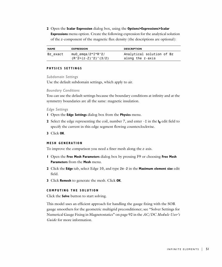
2 Open the Scalar Expression dialog box, using the Options>Expressions>Scalar
Expressions menu option. Create the following expression for the analytical solution of the z-component of the magnetic flux density (the descriptions are optional):
P H Y S I C S S E T T I N G S
Subdomain SettingsUse the default subdomain settings, which apply to air.
Boundary ConditionsYou can use the default settings because the boundary conditions at infinity and at the symmetry boundaries are all the same: magnetic insulation.
Edge Settings1 Open the Edge Settings dialog box from the Physics menu.
2 Select the edge representing the coil, number 7, and enter -I in the I0 edit field to specify the current in this edge segment flowing counterclockwise.
3 Click OK.
M E S H G E N E R A T I O N
To improve the comparison you need a finer mesh along the z-axis.
1 Open the Free Mesh Parameters dialog box by pressing F9 or choosing Free Mesh
Parameters from the Mesh menu.
2 Click the Edge tab, select Edge 10, and type 2e-2 in the Maximum element size edit field.
3 Click Remesh to generate the mesh. Click OK.
C O M P U T I N G T H E S O L U T I O N
Click the Solve button to start solving.
This model uses an efficient approach for handling the gauge fixing with the SOR gauge smoothers for the geometric multigrid preconditioner; see “Solver Settings for Numerical Gauge Fixing in Magnetostatics” on page 92 in the AC/DC Module User’s Guide for more information.
NAME EXPRESSION DESCRIPTION
Bz_exact mu0_emqa/2*I*R^2/(R^2+(z-Z)^2)^(3/2)
Analytical solution of Bz along the z-axis
I N F I N I T E E L E M E N T S | 51
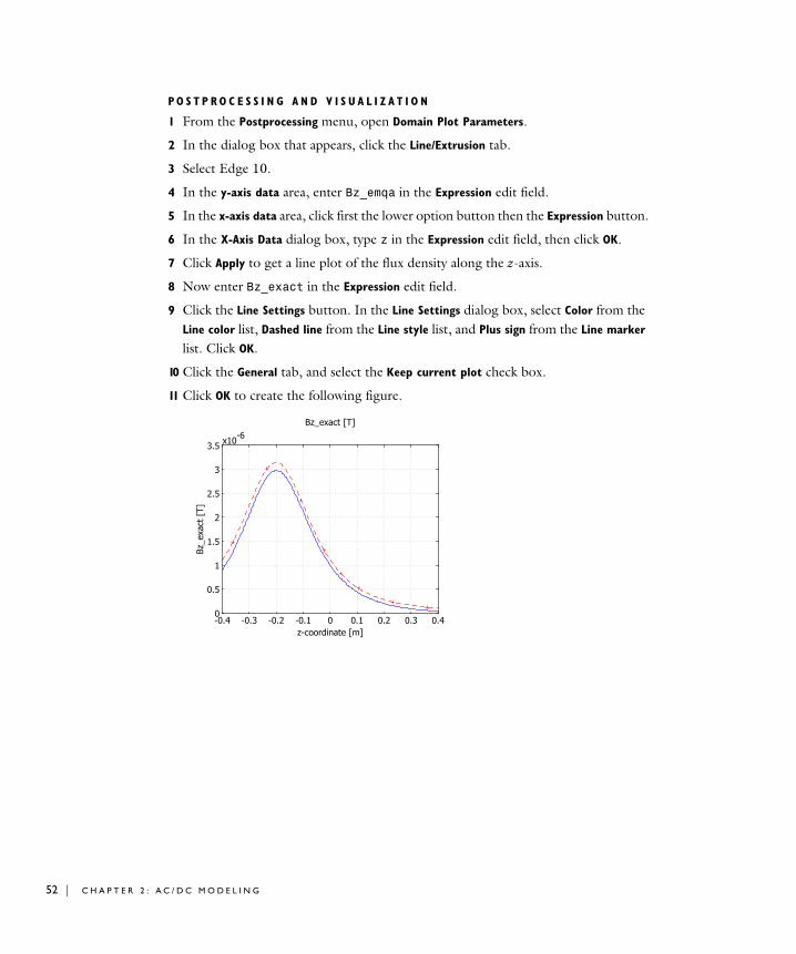
52 | C H A P T E R
PO S T P R O C E S S I N G A N D V I S U A L I Z A T I O N
1 From the Postprocessing menu, open Domain Plot Parameters.
2 In the dialog box that appears, click the Line/Extrusion tab.
3 Select Edge 10.
4 In the y-axis data area, enter Bz_emqa in the Expression edit field.
5 In the x-axis data area, click first the lower option button then the Expression button.
6 In the X-Axis Data dialog box, type z in the Expression edit field, then click OK.
7 Click Apply to get a line plot of the flux density along the z-axis.
8 Now enter Bz_exact in the Expression edit field.
9 Click the Line Settings button. In the Line Settings dialog box, select Color from the Line color list, Dashed line from the Line style list, and Plus sign from the Line marker list. Click OK.
10 Click the General tab, and select the Keep current plot check box.
11 Click OK to create the following figure.
2 : A C / D C M O D E L I N G
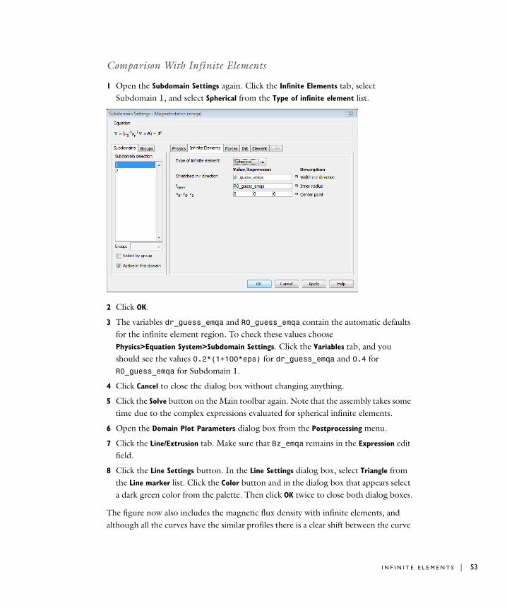
Comparison With Infinite Elements
1 Open the Subdomain Settings again. Click the Infinite Elements tab, select Subdomain 1, and select Spherical from the Type of infinite element list.
2 Click OK.
3 The variables dr_guess_emqa and R0_guess_emqa contain the automatic defaults for the infinite element region. To check these values choose Physics>Equation System>Subdomain Settings. Click the Variables tab, and you should see the values 0.2*(1+100*eps) for dr_guess_emqa and 0.4 for R0_guess_emqa for Subdomain 1.
4 Click Cancel to close the dialog box without changing anything.
5 Click the Solve button on the Main toolbar again. Note that the assembly takes some time due to the complex expressions evaluated for spherical infinite elements.
6 Open the Domain Plot Parameters dialog box from the Postprocessing menu.
7 Click the Line/Extrusion tab. Make sure that Bz_emqa remains in the Expression edit field.
8 Click the Line Settings button. In the Line Settings dialog box, select Triangle from the Line marker list. Click the Color button and in the dialog box that appears select a dark green color from the palette. Then click OK twice to close both dialog boxes.
The figure now also includes the magnetic flux density with infinite elements, and although all the curves have the similar profiles there is a clear shift between the curve
I N F I N I T E E L E M E N T S | 53
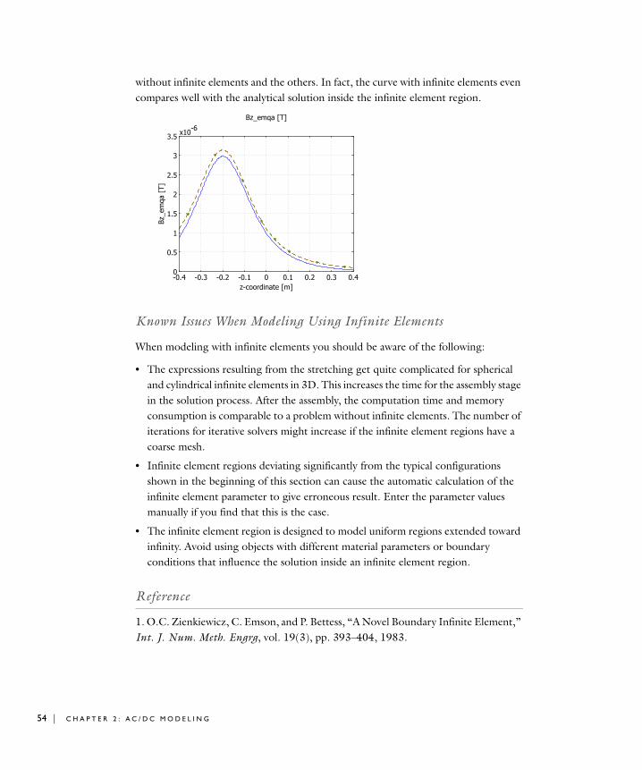
54 | C H A P T E R
without infinite elements and the others. In fact, the curve with infinite elements even compares well with the analytical solution inside the infinite element region.
Known Issues When Modeling Using Infinite Elements
When modeling with infinite elements you should be aware of the following:
• The expressions resulting from the stretching get quite complicated for spherical and cylindrical infinite elements in 3D. This increases the time for the assembly stage in the solution process. After the assembly, the computation time and memory consumption is comparable to a problem without infinite elements. The number of iterations for iterative solvers might increase if the infinite element regions have a coarse mesh.
• Infinite element regions deviating significantly from the typical configurations shown in the beginning of this section can cause the automatic calculation of the infinite element parameter to give erroneous result. Enter the parameter values manually if you find that this is the case.
• The infinite element region is designed to model uniform regions extended toward infinity. Avoid using objects with different material parameters or boundary conditions that influence the solution inside an infinite element region.
Reference
1. O.C. Zienkiewicz, C. Emson, and P. Bettess, “A Novel Boundary Infinite Element,” Int. J. Num. Meth. Engrg, vol. 19(3), pp. 393–404, 1983.
2 : A C / D C M O D E L I N G
Fo r c e and To r qu e Compu t a t i o n s
Computing Electromagnetic Forces and Torques
To compute electromagnetic forces and torques in COMSOL Multiphysics, two methods are available. This section describes one of them, which uses Maxwell’s stress tensor. There are also two functions, cemforce and cemtorque, which you can use when running COMSOL Multiphysics together with COMSOL Script or MATLAB. These functions use the method of virtual displacement to calculate the force and torque (see page 114 of the AC/DC Module Reference Guide).
Force and torque calculations using Maxwell’s stress tensor are available in the application modes for electrostatics, magnetostatics, and quasi-statics. In electrostatics the force is calculated by integrating
(2-1)
on the surface of the object that the force acts on. In magnetostatics and quasi-statics the expression
(2-2)
is integrated on the surface to obtain the force. E is the electric field, D the electric displacement, H the magnetic field, B the magnetic flux density, and n1 the outward normal from the object. For a theoretical discussion about the stress tensor see the section “Electromagnetic Forces” on page 110.
n1T212---n1 E D⋅( )– n1 E⋅( )DT
+=
n1T212---n1 H B⋅( )– n1 H⋅( )BT
+=
F O R C E A N D TO R Q U E C O M P U T A T I O N S | 55
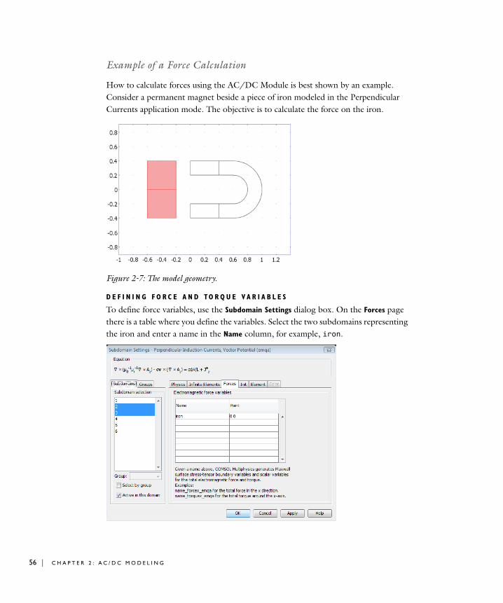
56 | C H A P T E R
Example of a Force Calculation
How to calculate forces using the AC/DC Module is best shown by an example. Consider a permanent magnet beside a piece of iron modeled in the Perpendicular Currents application mode. The objective is to calculate the force on the iron.
Figure 2-7: The model geometry.
D E F I N I N G F O R C E A N D TO R Q U E V A R I A B L E S
To define force variables, use the Subdomain Settings dialog box. On the Forces page there is a table where you define the variables. Select the two subdomains representing the iron and enter a name in the Name column, for example, iron.
2 : A C / D C M O D E L I N G
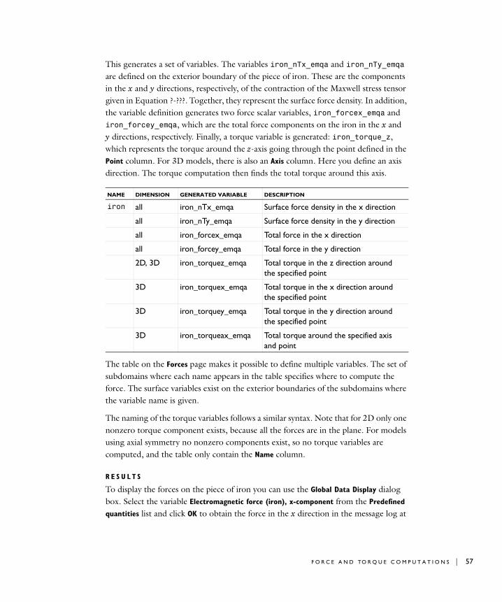
This generates a set of variables. The variables iron_nTx_emqa and iron_nTy_emqa are defined on the exterior boundary of the piece of iron. These are the components in the x and y directions, respectively, of the contraction of the Maxwell stress tensor given in Equation ?-???. Together, they represent the surface force density. In addition, the variable definition generates two force scalar variables, iron_forcex_emqa and iron_forcey_emqa, which are the total force components on the iron in the x and y directions, respectively. Finally, a torque variable is generated: iron_torque_z, which represents the torque around the z-axis going through the point defined in the Point column. For 3D models, there is also an Axis column. Here you define an axis direction. The torque computation then finds the total torque around this axis.
The table on the Forces page makes it possible to define multiple variables. The set of subdomains where each name appears in the table specifies where to compute the force. The surface variables exist on the exterior boundaries of the subdomains where the variable name is given.
The naming of the torque variables follows a similar syntax. Note that for 2D only one nonzero torque component exists, because all the forces are in the plane. For models using axial symmetry no nonzero components exist, so no torque variables are computed, and the table only contain the Name column.
R E S U L T S
To display the forces on the piece of iron you can use the Global Data Display dialog box. Select the variable Electromagnetic force (iron), x-component from the Predefined
quantities list and click OK to obtain the force in the x direction in the message log at
NAME DIMENSION GENERATED VARIABLE DESCRIPTION
iron all iron_nTx_emqa Surface force density in the x direction
all iron_nTy_emqa Surface force density in the y direction
all iron_forcex_emqa Total force in the x direction
all iron_forcey_emqa Total force in the y direction
2D, 3D iron_torquez_emqa Total torque in the z direction around the specified point
3D iron_torquex_emqa Total torque in the x direction around the specified point
3D iron_torquey_emqa Total torque in the y direction around the specified point
3D iron_torqueax_emqa Total torque around the specified axis and point
F O R C E A N D TO R Q U E C O M P U T A T I O N S | 57
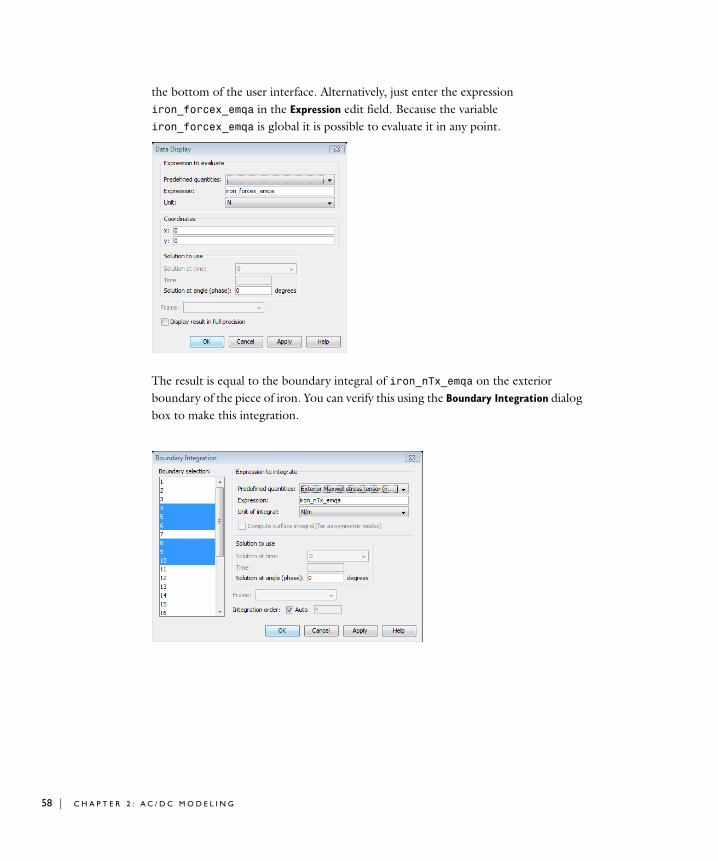
58 | C H A P T E R
the bottom of the user interface. Alternatively, just enter the expression iron_forcex_emqa in the Expression edit field. Because the variable iron_forcex_emqa is global it is possible to evaluate it in any point.
The result is equal to the boundary integral of iron_nTx_emqa on the exterior boundary of the piece of iron. You can verify this using the Boundary Integration dialog box to make this integration.
2 : A C / D C M O D E L I N G
Note: Because the force and torque variables are global, a conflict in variable names can occur if two application modes of the same type have the same suffix. Always make sure that the application mode suffix are different when you add extra application modes in other geometries.
Models Showing How to Compute Electromagnetic Forces
There are a number of examples in the AC/DC Module Model Library showing how to compute electromagnetic forces in different situations.
The models “Electromagnetic Forces on Parallel Current-Carrying Wires” on page 8 and “Linear Electric Motor of the Moving Coil Type” on page 30 in the AC/DC Module Model Library both show how to compute the total force on a device by integrating the volume force J × B. This is the most important method for computing forces in current-carrying devices. For materials that can be described as pure conductors (see later on in this section) this method gives the exact distribution of forces inside a device.
Additionally, “Linear Electric Motor of the Moving Coil Type” shows how to compute the force by the alternative method of virtual work, while “Electromagnetic Forces on Parallel Current-Carrying Wires” illustrates how to compute the force by integrating the Maxwell stress tensor on boundaries.
The model “Permanent Magnet” on page 21 in the AC/DC Module Model Library demonstrates how to compute the total force on a magnetizable rod close to a permanent magnet by integrating the Maxwell stress tensor in the air on the outside of the rod. This is the most important method for accurately computing the total force on magnetic devices for which the exact distribution of volume forces is not known. To retrieve the exact distribution of volume forces requires a material model that describes the interactions of the magnetizations and strains. Such material models are not always available. Therefore you are often limited to compute the total force by integrating the stress tensor or using the method of virtual work. Note that none of these methods allows you to compute and visualize the force distribution inside a domain, but only to compute the total force and torque in situations where the device is surrounded by air (or when this is a good approximation).
Torque calculations are used in “Generator with Mechanical Dynamics and Symmetry” on page 53 in the AC/DC Module Model Library.
F O R C E A N D TO R Q U E C O M P U T A T I O N S | 59

60 | C H A P T E R
2 : A C / D C M O D E L I N G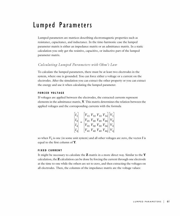
Lumped Pa r ame t e r s
Lumped parameters are matrices describing electromagnetic properties such as resistance, capacitance, and inductance. In the time-harmonic case the lumped parameter matrix is either an impedance matrix or an admittance matrix. In a static calculation you only get the resistive, capacitive, or inductive part of the lumped parameter matrix.
Calculating Lumped Parameters with Ohm’s Law
To calculate the lumped parameters, there must be at least two electrodes in the system, where one is grounded. You can force either a voltage or a current on the electrodes. After the simulation you can extract the other property or you can extract the energy and use it when calculating the lumped parameter.
F O R C E D VO L T A G E
If voltages are applied between the electrodes, the extracted currents represent elements in the admittance matrix, Y. This matrix determines the relation between the applied voltages and the corresponding currents with the formula
so when V1 is one (in some unit system) and all other voltages are zero, the vector I is equal to the first column of Y.
F I X E D C U R R E N T
It might be necessary to calculate the Z-matrix in a more direct way. Similar to the Y calculation, the Z calculation can be done by forcing the current through one electrode at the time to one while the others are set to zero, and then extracting the voltages on all electrodes. Then, the columns of the impedance matrix are the voltage values:
I1
I2
I4
I4
Y11 Y12 Y13 Y14
Y21 Y22 Y23 Y24
Y31 Y32 Y33 Y34
Y41 Y42 Y43 Y44
V1
V2
V3
V4
=
L U M P E D P A R A M E T E R S | 61
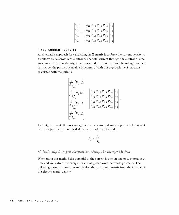
62 | C H A P T E R
F I X E D C U R R E N T D E N S I T Y
An alternative approach for calculating the Z-matrix is to force the current density to a uniform value across each electrode. The total current through the electrode is the area times the current density, which is selected to be one or zero. The voltage can then vary across the port, so averaging is necessary. With this approach the Z-matrix is calculated with the formula
.
Here An represents the area and In the normal current density of port n. The current density is just the current divided by the area of that electrode.
Calculating Lumped Parameters Using the Energy Method
When using this method the potential or the current is one on one or two ports at a time and you extract the energy density integrated over the whole geometry. The following formulas show how to calculate the capacitance matrix from the integral of the electric energy density.
V1
V2
V3
V4
Z11 Z12 Z13 Z14
Z21 Z22 Z23 Z24
Z31 Z32 Z33 Z34
Z41 Z42 Z43 Z44
I1
I2
I3
I4
=
1A1------- V1 Ad
A1
∫1
A2------- V2 Ad
A2
∫1
A3------- V3 Ad
A3
∫1
A4------- V4 Ad
A4
∫
Z11 Z12 Z13 Z14
Z21 Z22 Z23 Z24
Z31 Z32 Z33 Z34
Z41 Z42 Z43 Z44
I1
I2
I3
I4
=
JnIn
An-------=
2 : A C / D C M O D E L I N G
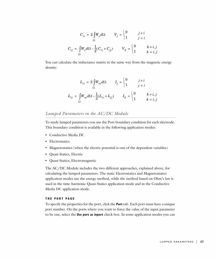
You can calculate the inductance matrix in the same way from the magnetic energy density:
Lumped Parameters in the AC/DC Module
To study lumped parameters you use the Port boundary condition for each electrode. This boundary condition is available in the following application modes:
• Conductive Media DC
• Electrostatics
• Magnetostatics (when the electric potential is one of the dependent variables)
• Quasi-Statics, Electric
• Quasi-Statics, Electromagnetic
The AC/DC Module includes the two different approaches, explained above, for calculating the lumped parameters. The static Electrostatics and Magnetostatics application modes use the energy method, while the method based on Ohm’s law is used in the time-harmonic Quasi-Statics application mode and in the Conductive Media DC application mode.
T H E PO R T P A G E
To specify the properties for the port, click the Port tab. Each port must have a unique port number. On the ports where you want to force the value of the input parameter to be one, select the Use port as inport check box. In some application modes you can
Cii 2 We ΩdΩ∫= Vj
01⎩
⎨⎧
= j i≠j i=
Cij We ΩdΩ∫ 1
2--- Cii Cjj+( )–= Vk
01⎩
⎨⎧
= k i j,≠k i j,=
Lii 2 Wm ΩdΩ∫= Ij
01⎩
⎨⎧
= j i≠j i=
Lij Wm ΩdΩ∫ 1
2--- Lii Ljj+( )–= Ik
01⎩
⎨⎧
= k i j,≠k i j,=
L U M P E D P A R A M E T E R S | 63
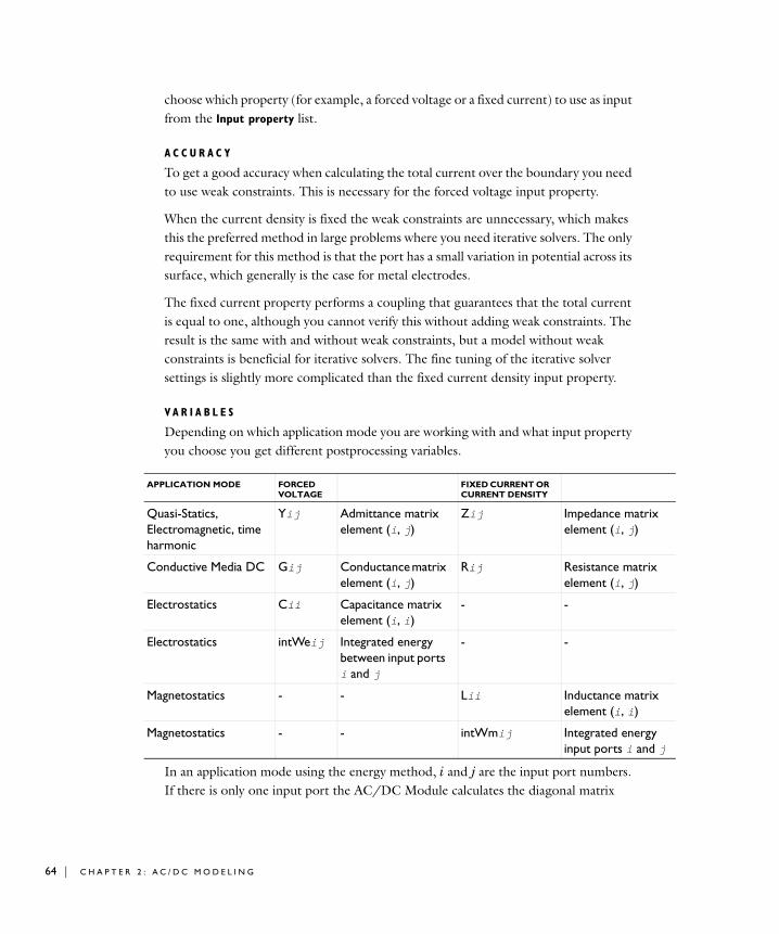
64 | C H A P T E R
ix
x
ix
y d j
choose which property (for example, a forced voltage or a fixed current) to use as input from the Input property list.
A C C U R A C Y
To get a good accuracy when calculating the total current over the boundary you need to use weak constraints. This is necessary for the forced voltage input property.
When the current density is fixed the weak constraints are unnecessary, which makes this the preferred method in large problems where you need iterative solvers. The only requirement for this method is that the port has a small variation in potential across its surface, which generally is the case for metal electrodes.
The fixed current property performs a coupling that guarantees that the total current is equal to one, although you cannot verify this without adding weak constraints. The result is the same with and without weak constraints, but a model without weak constraints is beneficial for iterative solvers. The fine tuning of the iterative solver settings is slightly more complicated than the fixed current density input property.
VA R I A B L E S
Depending on which application mode you are working with and what input property you choose you get different postprocessing variables.
In an application mode using the energy method, i and j are the input port numbers. If there is only one input port the AC/DC Module calculates the diagonal matrix
APPLICATION MODE FORCED VOLTAGE
FIXED CURRENT OR CURRENT DENSITY
Quasi-Statics, Electromagnetic, time harmonic
Yij Admittance matrix element (i, j)
Zij Impedance matrelement (i, j)
Conductive Media DC Gij Conductance matrix element (i, j)
Rij Resistance matrielement (i, j)
Electrostatics Cii Capacitance matrix element (i, i)
- -
Electrostatics intWeij Integrated energy between input ports i and j
- -
Magnetostatics - - Lii Inductance matrelement (i, i)
Magnetostatics - - intWmij Integrated energinput ports i an
2 : A C / D C M O D E L I N G
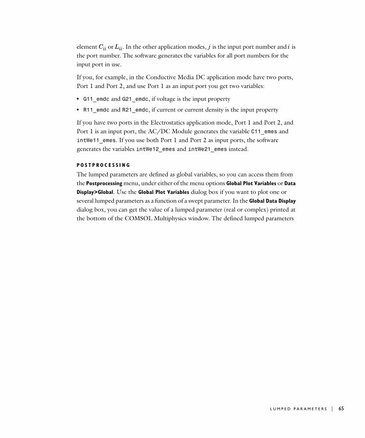
element Cii or Lii. In the other application modes, j is the input port number and i is the port number. The software generates the variables for all port numbers for the input port in use.
If you, for example, in the Conductive Media DC application mode have two ports, Port 1 and Port 2, and use Port 1 as an input port you get two variables:
• G11_emdc and G21_emdc, if voltage is the input property
• R11_emdc and R21_emdc, if current or current density is the input property
If you have two ports in the Electrostatics application mode, Port 1 and Port 2, and Port 1 is an input port, the AC/DC Module generates the variable C11_emes and intWe11_emes. If you use both Port 1 and Port 2 as input ports, the software generates the variables intWe12_emes and intWe21_emes instead.
PO S T P R O C E S S I N G
The lumped parameters are defined as global variables, so you can access them from the Postprocessing menu, under either of the menu options Global Plot Variables or Data
Display>Global. Use the Global Plot Variables dialog box if you want to plot one or several lumped parameters as a function of a swept parameter. In the Global Data Display dialog box, you can get the value of a lumped parameter (real or complex) printed at the bottom of the COMSOL Multiphysics window. The defined lumped parameters
L U M P E D P A R A M E T E R S | 65
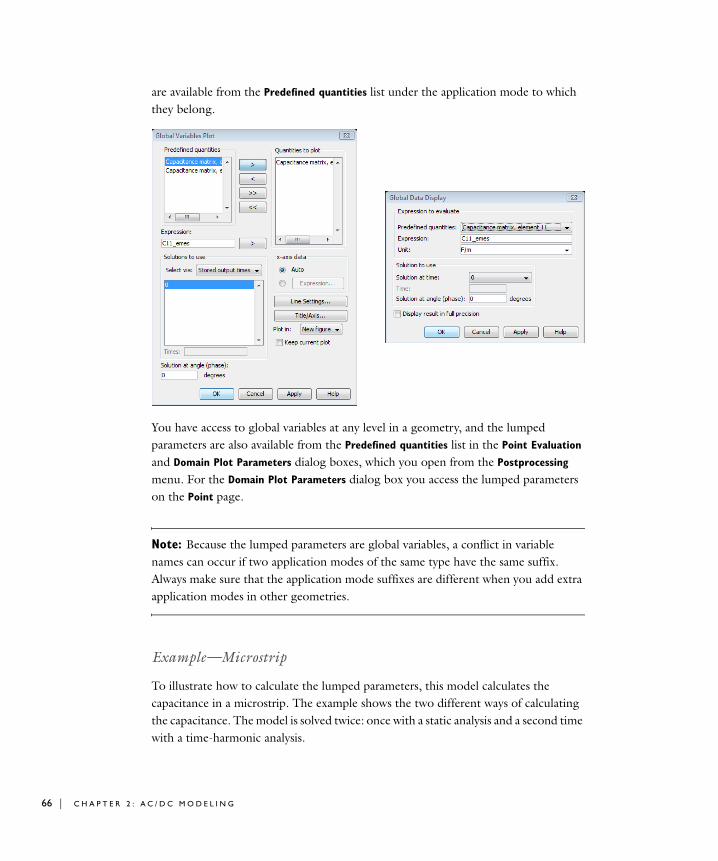
66 | C H A P T E R
are available from the Predefined quantities list under the application mode to which they belong.
You have access to global variables at any level in a geometry, and the lumped parameters are also available from the Predefined quantities list in the Point Evaluation and Domain Plot Parameters dialog boxes, which you open from the Postprocessing menu. For the Domain Plot Parameters dialog box you access the lumped parameters on the Point page.
Note: Because the lumped parameters are global variables, a conflict in variable names can occur if two application modes of the same type have the same suffix. Always make sure that the application mode suffixes are different when you add extra application modes in other geometries.
Example—Microstrip
To illustrate how to calculate the lumped parameters, this model calculates the capacitance in a microstrip. The example shows the two different ways of calculating the capacitance. The model is solved twice: once with a static analysis and a second time with a time-harmonic analysis.
2 : A C / D C M O D E L I N G
R E S U L T S
When making a static analysis you get the capacitance directly as a variable. When solving the time-harmonic problem you need to calculate the capacitance from the admittance by dividing the imaginary part of the admittance with the angular frequency.
Model Library path: ACDC_Module/Tutorial_Models/microstrip
Modeling Using the Graphical User Interface
M O D E L N A V I G A T O R
1 In the Model Navigator, select 2D from the Space dimension list.
2 Open the AC/DC Module folder, then select Statics>Electrostatics.
3 Click OK.
G E O M E T R Y M O D E L I N G
1 Select Specify Objects>Rectangle from the Draw menu.
2 Type 1.5e-3 in the Width edit field and type 6.45e-4 in the Height edit field.
3 Click OK.
4 Click the Zoom Extents button on the Main toolbar.
1 Select Specify Objects>Rectangle from the Draw menu.
2 Type 3.3e-4 in the Width edit field and 3.56e-5 in the Height edit field.
3 In the Position area, type 6e-4 in the x edit field and 3.05e-4 in the y edit field.
4 Click OK.
5 Press Ctrl+A to select both rectangles.
6 Click the Difference button on the Draw toolbar.
P H Y S I C S S E T T I N G S
Subdomain Settings1 Open the Subdomain Settings dialog box.
C Im Y( )ω
-----------------=
L U M P E D P A R A M E T E R S | 67
68 | C H A P T E R
2 Select Subdomain 1 and set the relative permittivity to 3.25.
3 Click OK.
Boundary Conditions1 Open the Boundary Settings dialog box.
2 Select Boundaries 1 and 8 and set the boundary condition to Zero charge/Symmetry.
3 Set the boundary condition on Boundaries 4–7 to Port.
4 Click the Port tab and select the Use port as input check box.
5 Click OK.
Application Mode Properties1 Open the Application Mode Properties dialog box by selecting Properties from the
Physics menu.
2 Select On from the Weak constraints list, then click OK.
M E S H G E N E R A T I O N A N D S O L U T I O N
1 Initialize the mesh and refine it once.
2 Solve with the default settings.
PO S T P R O C E S S I N G
1 Select Point evaluation from the Postprocessing menu.
2 Select Capacitance matrix, element 11 in the Predefined quantities list, select Point 1, and click OK to see the capacitance value in the message log.
T I M E - H A R M O N I C A N A L Y S I S
1 Open the Model Navigator from the Multiphysics menu.
2 Select Quasi-Statics, Electromagnetic>In-Plane Electric and Induction Currents,
Potentials>Time-harmonic analysis.
3 Click Add, then click OK.
P H Y S I C S S E T T I N G S
Subdomain Settings1 Open the Subdomain Settings dialog box.
2 Select Subdomain 1 and click the Electric Parameters tab.
3 Set the relative permittivity to 3.25, then click OK.
2 : A C / D C M O D E L I N G
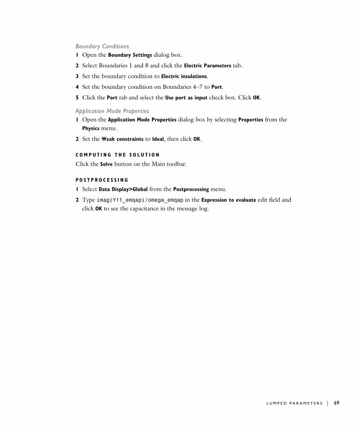
Boundary Conditions1 Open the Boundary Settings dialog box.
2 Select Boundaries 1 and 8 and click the Electric Parameters tab.
3 Set the boundary condition to Electric insulations.
4 Set the boundary condition on Boundaries 4–7 to Port.
5 Click the Port tab and select the Use port as input check box. Click OK.
Application Mode Properties1 Open the Application Mode Properties dialog box by selecting Properties from the
Physics menu.
2 Set the Weak constraints to Ideal, then click OK.
C O M P U T I N G T H E S O L U T I O N
Click the Solve button on the Main toolbar.
PO S T P R O C E S S I N G
1 Select Data Display>Global from the Postprocessing menu.
2 Type imag(Y11_emqap)/omega_emqap in the Expression to evaluate edit field and click OK to see the capacitance in the message log.
L U M P E D P A R A M E T E R S | 69
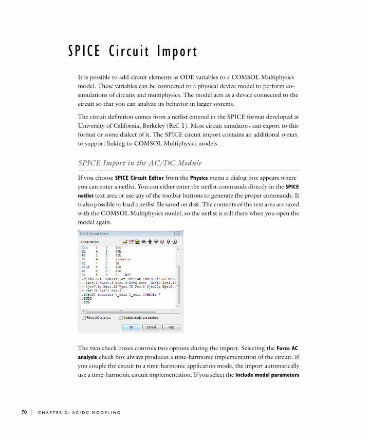
70 | C H A P T E R
S P I C E C i r c u i t Impo r t
It is possible to add circuit elements as ODE variables to a COMSOL Multiphysics model. These variables can be connected to a physical device model to perform co-simulations of circuits and multiphysics. The model acts as a device connected to the circuit so that you can analyze its behavior in larger systems.
The circuit definition comes from a netlist entered in the SPICE format developed at University of California, Berkeley (Ref. 1). Most circuit simulators can export to this format or some dialect of it. The SPICE circuit import contains an additional syntax to support linking to COMSOL Multiphysics models.
SPICE Import in the AC/DC Module
If you choose SPICE Circuit Editor from the Physics menu a dialog box appears where you can enter a netlist. You can either enter the netlist commands directly in the SPICE
netlist text area or use any of the toolbar buttons to generate the proper commands. It is also possible to load a netlist file saved on disk. The contents of the text area are saved with the COMSOL Multiphysics model, so the netlist is still there when you open the model again.
The two check boxes controls two options during the import. Selecting the Force AC
analysis check box always produces a time-harmonic implementation of the circuit. If you couple the circuit to a time-harmonic application mode, the import automatically use a time-harmonic circuit implementation. If you select the Include model parameters
2 : A C / D C M O D E L I N G
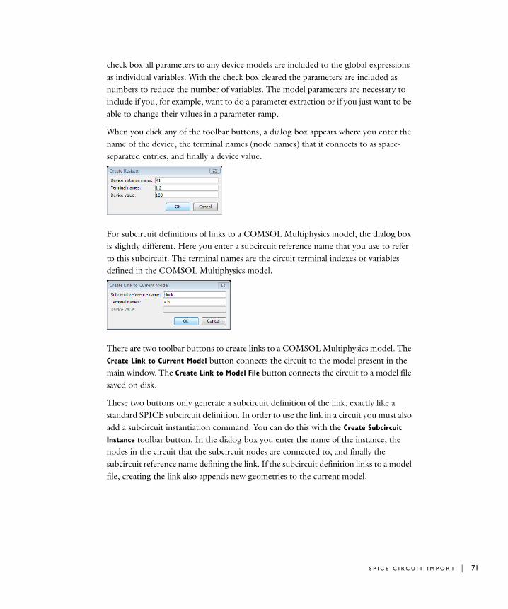
check box all parameters to any device models are included to the global expressions as individual variables. With the check box cleared the parameters are included as numbers to reduce the number of variables. The model parameters are necessary to include if you, for example, want to do a parameter extraction or if you just want to be able to change their values in a parameter ramp.
When you click any of the toolbar buttons, a dialog box appears where you enter the name of the device, the terminal names (node names) that it connects to as space-separated entries, and finally a device value.
For subcircuit definitions of links to a COMSOL Multiphysics model, the dialog box is slightly different. Here you enter a subcircuit reference name that you use to refer to this subcircuit. The terminal names are the circuit terminal indexes or variables defined in the COMSOL Multiphysics model.
There are two toolbar buttons to create links to a COMSOL Multiphysics model. The Create Link to Current Model button connects the circuit to the model present in the main window. The Create Link to Model File button connects the circuit to a model file saved on disk.
These two buttons only generate a subcircuit definition of the link, exactly like a standard SPICE subcircuit definition. In order to use the link in a circuit you must also add a subcircuit instantiation command. You can do this with the Create Subcircuit
Instance toolbar button. In the dialog box you enter the name of the instance, the nodes in the circuit that the subcircuit nodes are connected to, and finally the subcircuit reference name defining the link. If the subcircuit definition links to a model file, creating the link also appends new geometries to the current model.
S P I C E C I R C U I T I M P O R T | 71
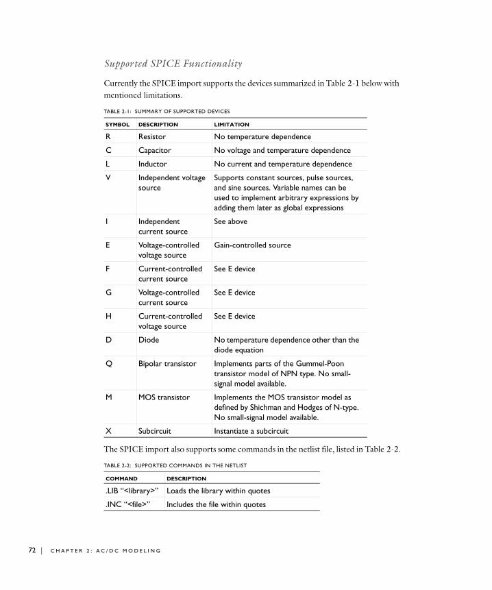
72 | C H A P T E R
Supported SPICE Functionality
Currently the SPICE import supports the devices summarized in Table 2-1 below with mentioned limitations.
The SPICE import also supports some commands in the netlist file, listed in Table 2-2.
TABLE 2-1: SUMMARY OF SUPPORTED DEVICES
SYMBOL DESCRIPTION LIMITATION
R Resistor No temperature dependence
C Capacitor No voltage and temperature dependence
L Inductor No current and temperature dependence
V Independent voltage source
Supports constant sources, pulse sources, and sine sources. Variable names can be used to implement arbitrary expressions by adding them later as global expressions
I Independent current source
See above
E Voltage-controlled voltage source
Gain-controlled source
F Current-controlled current source
See E device
G Voltage-controlled current source
See E device
H Current-controlled voltage source
See E device
D Diode No temperature dependence other than the diode equation
Q Bipolar transistor Implements parts of the Gummel-Poon transistor model of NPN type. No small-signal model available.
M MOS transistor Implements the MOS transistor model as defined by Shichman and Hodges of N-type. No small-signal model available.
X Subcircuit Instantiate a subcircuit
TABLE 2-2: SUPPORTED COMMANDS IN THE NETLIST
COMMAND DESCRIPTION
.LIB “<library>” Loads the library within quotes
.INC “<file>” Includes the file within quotes
2 : A C / D C M O D E L I N G
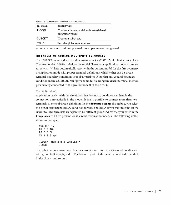
All other commands and unsupported model parameters are ignored.
I N S T A N C E S O F C O M S O L M U L T I P H Y S I C S M O D E L S
The .SUBCKT command also handles instances of COMSOL Multiphysics model files. The extra option COMSOL: defines the model filename or application mode to link to. An asterisk (*) here automatically searches in the current model for the first geometry or application mode with proper terminal definitions, which either can be circuit terminal boundary conditions or global variables. Note that any ground boundary condition in the COMSOL Multiphysics model file using the circuit terminal method gets directly connected to the ground node 0 of the circuit.
Circuit TerminalsApplication modes with the circuit terminal boundary condition can handle the connection automatically in the model. It is also possible to connect more than two terminals to one subcircuit definition. In the Boundary Settings dialog box, you select the circuit terminal boundary condition for those boundaries you want to connect the circuit to. The terminals are separated by different group indices that you enter in the Group index edit field present for all circuit terminal boundaries. The following netlist shows an example:
Vin 0 1 1VR1 0 2 10kR2 0 310kX1 1 2 3 mph
.SUBCKT mph a b c COMSOL: *
.ENDS
The subcircuit command searches the current model for circuit terminal conditions with group indices a, b, and c. The boundary with index a gets connected to node 1 in the circuit, and so on.
.MODEL Creates a device model with user-defined parameter values
.SUBCKT Creates a subcircuit
.TEMP Sets the global temperature
TABLE 2-2: SUPPORTED COMMANDS IN THE NETLIST
COMMAND DESCRIPTION
S P I C E C I R C U I T I M P O R T | 73
74 | C H A P T E R
Note: The circuit terminal boundary condition is actually identical to the floating potential boundary condition, but without possibility to specify the current. The SPICE Import dialog automatically specifies the current to a circuit terminal to be controlled by the circuit. You can also use the floating potential boundary conditions for circuit connections.
Terminal VariablesApplication modes without the circuit terminal boundary conditions need two variables: one for device voltage and one for device current. The names of these variables are passed to the .SUBCKT command after the name of the device. If there are more than two terminals in the model file, you must define one subcircuit for each voltage-current pair. The following netlist shows a simple example when using terminal variables:
Vin 0 2 1VR1 2 1 10kX1 1 0 Rfem.SUBSCKT Rfem V_res I_res COMSOL: Rmodel.mph.ENDS
This circuit connects the finite element model in the file Rmodel.mph to a circuit with a voltage source Vin and a resistor R1 through the instance X1. The model file Rmodel.mph has two variables, V_res and I_res, defined in the global scope. The variable I_res must be a variable defined in the Global Variables dialog box, because it is altered by the SPICE Import. The instance X1 is connected to nodes 1 and 0, and the voltage between these nodes is made equal to V_res, by changing the current I_res. I_res controls the current from node 1 to node 0.
If the second variable begins with one of the letters V, v, U, or u, COMSOL Multiphysics defines the circuit so it controls the voltage and reads the current. It is always the second variable that has to be present in the Global Variables dialog box, which in this case is interpreted as a voltage. This approach can generate less ODE variables for models where it is easier to give the voltage and calculate the current.
Note: The number of instances of a model file that you can use in a circuit is limited to one for the terminal variable approach. Using additional instances causes variable-name conflicts. The circuit terminal approach can use several instances.
2 : A C / D C M O D E L I N G
L I M I T A T I O N S O F T H E S P I C E I M P O R T
Not all device models are implemented, and those implemented do not support the full range of parameters available. Table 2-1 lists the supported devices. You might therefore have to simplify the netlist prior to the import. In addition, support for model parameters specifying a temperature dependence is not implemented. However, the temperature affects the leakage current on all modeled p-n junctions according to the diode equation.
The transit-time capacitance is not supported for the semiconductor device models where it is used.
All statements for specifying input signals are not supported. Currently the supported statements are SIN and PULSE.
The SPICE import does not support small-signal analysis of semiconductor device models. In a time-harmonic simulation you can only connect sources and passive devices.
S C R I P T S U P P O R T
You can also access the functionality described in the preceding section from COMSOL Script using the spiceimport command; see the chapter “Function Reference” on page 111 in the AC/DC Module Reference Guide.
Reference
1. http://bwrc.eecs.berkeley.edu/Classes/IcBook/SPICE/
Example Models using SPICE Import
There are two models in the model library that use SPICE Import. The model “High Current Cables in a Circuit” on page 170 in the AC/DC Module Model Library uses the circuit terminal approach, and the model “Inductor in Amplifier Circuit” on page 189 in the same manual is an example of the terminal variable approach.
S P I C E C I R C U I T I M P O R T | 75
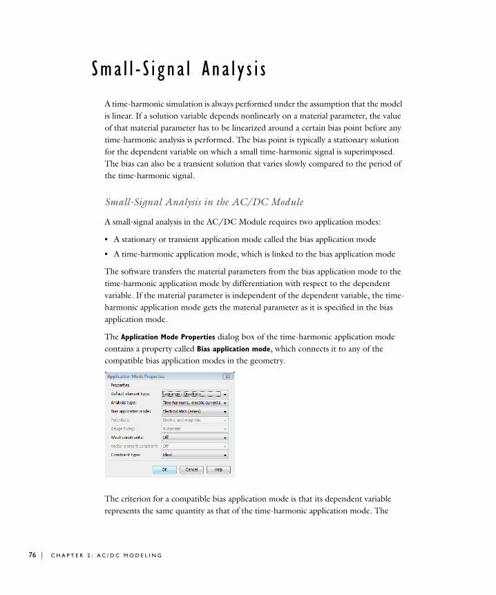
76 | C H A P T E R
Sma l l - S i g n a l Ana l y s i s
A time-harmonic simulation is always performed under the assumption that the model is linear. If a solution variable depends nonlinearly on a material parameter, the value of that material parameter has to be linearized around a certain bias point before any time-harmonic analysis is performed. The bias point is typically a stationary solution for the dependent variable on which a small time-harmonic signal is superimposed. The bias can also be a transient solution that varies slowly compared to the period of the time-harmonic signal.
Small-Signal Analysis in the AC/DC Module
A small-signal analysis in the AC/DC Module requires two application modes:
• A stationary or transient application mode called the bias application mode
• A time-harmonic application mode, which is linked to the bias application mode
The software transfers the material parameters from the bias application mode to the time-harmonic application mode by differentiation with respect to the dependent variable. If the material parameter is independent of the dependent variable, the time-harmonic application mode gets the material parameter as it is specified in the bias application mode.
The Application Mode Properties dialog box of the time-harmonic application mode contains a property called Bias application mode, which connects it to any of the compatible bias application modes in the geometry.
The criterion for a compatible bias application mode is that its dependent variable represents the same quantity as that of the time-harmonic application mode. The
2 : A C / D C M O D E L I N G
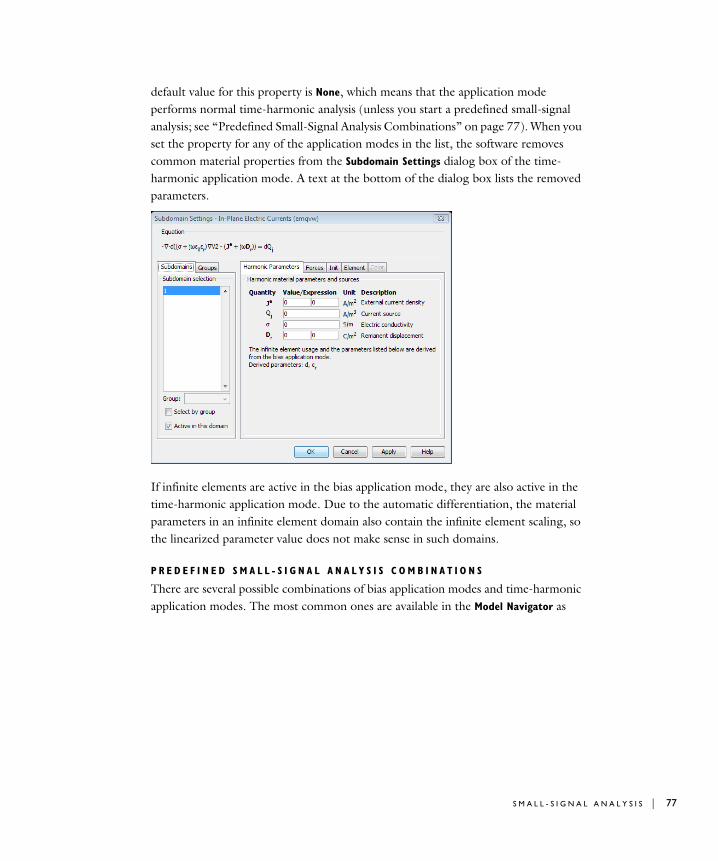
default value for this property is None, which means that the application mode performs normal time-harmonic analysis (unless you start a predefined small-signal analysis; see “Predefined Small-Signal Analysis Combinations” on page 77). When you set the property for any of the application modes in the list, the software removes common material properties from the Subdomain Settings dialog box of the time-harmonic application mode. A text at the bottom of the dialog box lists the removed parameters.
If infinite elements are active in the bias application mode, they are also active in the time-harmonic application mode. Due to the automatic differentiation, the material parameters in an infinite element domain also contain the infinite element scaling, so the linearized parameter value does not make sense in such domains.
P R E D E F I N E D S M A L L - S I G N A L A N A L Y S I S C O M B I N A T I O N S
There are several possible combinations of bias application modes and time-harmonic application modes. The most common ones are available in the Model Navigator as
S M A L L - S I G N A L A N A L Y S I S | 77
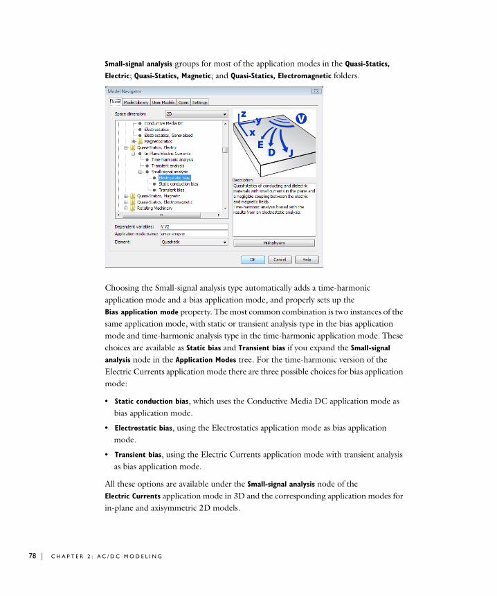
78 | C H A P T E R
Small-signal analysis groups for most of the application modes in the Quasi-Statics,
Electric; Quasi-Statics, Magnetic; and Quasi-Statics, Electromagnetic folders.
Choosing the Small-signal analysis type automatically adds a time-harmonic application mode and a bias application mode, and properly sets up the Bias application mode property. The most common combination is two instances of the same application mode, with static or transient analysis type in the bias application mode and time-harmonic analysis type in the time-harmonic application mode. These choices are available as Static bias and Transient bias if you expand the Small-signal
analysis node in the Application Modes tree. For the time-harmonic version of the Electric Currents application mode there are three possible choices for bias application mode:
• Static conduction bias, which uses the Conductive Media DC application mode as bias application mode.
• Electrostatic bias, using the Electrostatics application mode as bias application mode.
• Transient bias, using the Electric Currents application mode with transient analysis as bias application mode.
All these options are available under the Small-signal analysis node of the Electric Currents application mode in 3D and the corresponding application modes for in-plane and axisymmetric 2D models.
2 : A C / D C M O D E L I N G
M O D E L I N G S T E P S
Although it is possible to do the calculation in one step, it is recommended to do it in separate steps. Especially if you are doing a parameter sweep or solving a large model. The model is always one-way coupled from the bias application mode to the time-harmonic application mode. The following steps describe the recommended procedure:
1 Try to find an appropriate small-signal analysis combination in the Model Navigator window. Otherwise, use the Multiphysics and Add buttons to create your own valid combination.
2 Finish all modeling steps defining variables, physics settings, and mesh.
3 Use the Solver Manager dialog box to solve only for the bias application mode. If you are doing a parameter sweep, solve for all parameters for this application mode.
4 Go back to the Solver Manager dialog box, click the Store Solution button, and store all solutions. On the Initial Value page, use Stored solution as the linearization point, and choose All from the Solution at time list. This ensures that the subsequent parameter sweep uses the correct solution of the bias application mode for each parameter step.
5 Repeat the solve step, solving only for the time-harmonic application mode. The final solution contains the bias solution and the time-harmonic solution as separate variables. The nonlinear material parameters are differentiated at each parameter step with respect to the bias solution in that step.
Example—Small-Signal Analysis of an Inductor
This example uses the model “Inductor in Amplifier Circuit” on page 189 of the AC/DC Module Model Library before the SPICE Import. This model consists of an inductor with a nonlinear magnetic core that shows a changing inductance when the current increases. In this example you investigate the small-signal inductance as a function of current through the inductor.
Model Library path: AC/DC_Module/Tutorial_Models/small_signal_analysis_of_inductor
S M A L L - S I G N A L A N A L Y S I S | 79
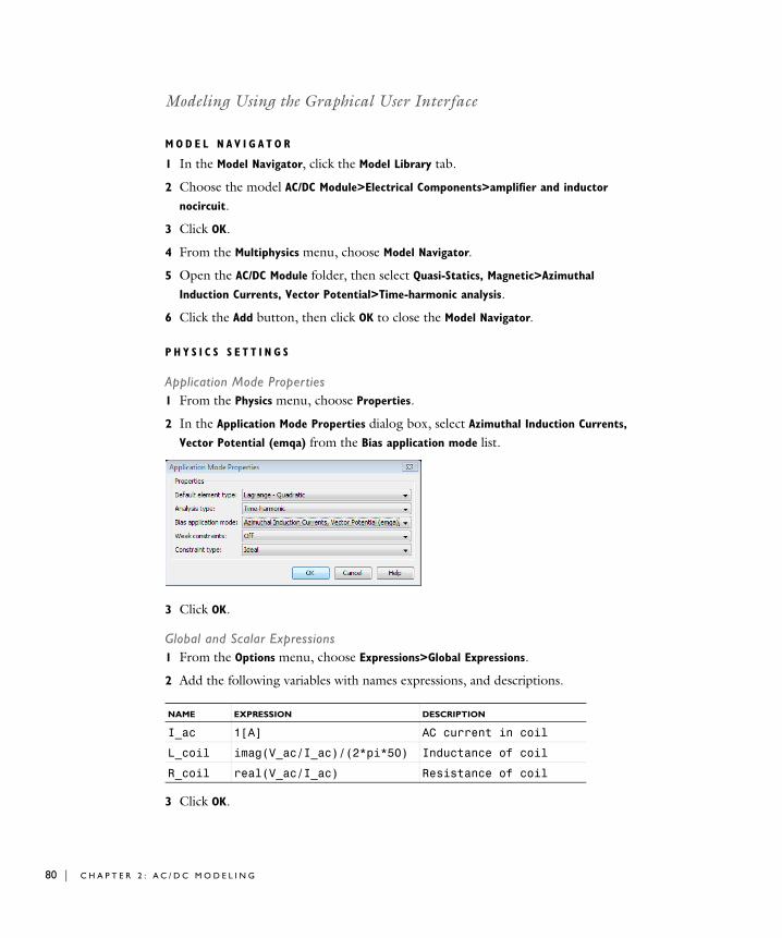
80 | C H A P T E R
Modeling Using the Graphical User Interface
M O D E L N A V I G A T O R
1 In the Model Navigator, click the Model Library tab.
2 Choose the model AC/DC Module>Electrical Components>amplifier and inductor
nocircuit.
3 Click OK.
4 From the Multiphysics menu, choose Model Navigator.
5 Open the AC/DC Module folder, then select Quasi-Statics, Magnetic>Azimuthal
Induction Currents, Vector Potential>Time-harmonic analysis.
6 Click the Add button, then click OK to close the Model Navigator.
P H Y S I C S S E T T I N G S
Application Mode Properties1 From the Physics menu, choose Properties.
2 In the Application Mode Properties dialog box, select Azimuthal Induction Currents,
Vector Potential (emqa) from the Bias application mode list.
3 Click OK.
Global and Scalar Expressions1 From the Options menu, choose Expressions>Global Expressions.
2 Add the following variables with names expressions, and descriptions.
3 Click OK.
NAME EXPRESSION DESCRIPTION
I_ac 1[A] AC current in coil
L_coil imag(V_ac/I_ac)/(2*pi*50) Inductance of coil
R_coil real(V_ac/I_ac) Resistance of coil
2 : A C / D C M O D E L I N G
4 From the Options menu, choose Expressions>Scalar Expressions.
5 Add a variable named J_ac with the expression I_ac*N/A.
6 Click OK.
Integration Coupling Variables1 From the Options menu, choose Integration Coupling Variables>Subdomain Variables.
2 In the Subdomain Integration Variables dialog box, add a variable named V_ac according to the table below.
3 Click OK.
Subdomain Settings1 Open the Subdomain Settings dialog box from the Physics menu.
2 Select Subdomain 3 and enter J_ac in the edit field for the external current density.
3 Click OK. Note that some material parameters are inherited from the bias application mode settings.
Boundary Conditions1 Open the Boundary Settings dialog box from the Physics menu.
2 Select Boundaries 1, 2 and 4. Set the Boundary condition to Axial symmetry.
3 Click OK.
M E S H G E N E R A T I O N
Use the mesh of the original model.
C O M P U T I N G T H E S O L U T I O N
Although both the bias application mode and the time-harmonic application mode can be solved simultaneously, the following steps show how to solve them separately. This is done to illustrate the correct procedure for solving larger-size problems.
1 From the Solve menu, open the Solver Parameters dialog box.
2 From the Solver list, choose Parametric.
3 Type I_coil in the Parameter name edit field and 1:0.2:10 in the Parameter values edit field.
4 Click OK.
5 From the Solve menu, open the Solver Manager.
NAME EXPRESSION IN SUBDOMAIN 3
V_ac N*2*pi*r*(I_ac/(sigma_coil*pi*r_coil^2)-Ephi_emqa2)/A
S M A L L - S I G N A L A N A L Y S I S | 81
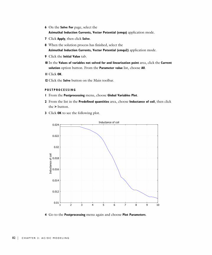
82 | C H A P T E R
6 On the Solve For page, select the Azimuthal Induction Currents, Vector Potential (emqa) application mode.
7 Click Apply, then click Solve.
8 When the solution process has finished, select the Azimuthal Induction Currents, Vector Potential (emqa2) application mode.
9 Click the Initial Value tab.
10 In the Values of variables not solved for and linearization point area, click the Current
solution option button. From the Parameter value list, choose All.
11 Click OK.
12 Click the Solve button on the Main toolbar.
PO S T P R O C E S S I N G
1 From the Postprocessing menu, choose Global Variables Plot.
2 From the list in the Predefined quantities area, choose Inductance of coil, then click the > button.
3 Click OK to see the following plot.
4 Go to the Postprocessing menu again and choose Plot Parameters.
2 : A C / D C M O D E L I N G
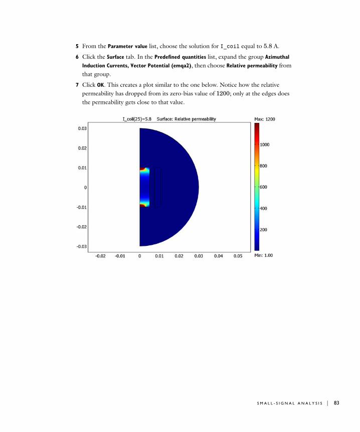
5 From the Parameter value list, choose the solution for I_coil equal to 5.8 A.
6 Click the Surface tab. In the Predefined quantities list, expand the group Azimuthal
Induction Currents, Vector Potential (emqa2), then choose Relative permeability from that group.
7 Click OK. This creates a plot similar to the one below. Notice how the relative permeability has dropped from its zero-bias value of 1200; only at the edges does the permeability gets close to that value.
S M A L L - S I G N A L A N A L Y S I S | 83
84 | C H A P T E R
S o l v i n g L a r g e 3D P r ob l em s
For large 3D electromagnetic problems, where the default direct linear solver requires too much memory, you can use the iterative linear solver GMRES together with the Geometric multigrid (GMG) preconditioner for problems without gauge fixing. For gauge fixed electromagnetic problems you can use GMG as iterative linear solver and the Vanka preconditioner as presmoother and postsmoother. Gauge fixing is necessary for magnetostatic problems in 3D and quasi-static problems when solving for the magnetic vector potential and the electric potential. Note that for magnetostatic problems an alternative to explicit gauge fixing exists. This alternative consists of fixing the gauge numerically with one of the SOR gauge smoothers. This section describes how to use the iterative solvers in the context of the mentioned problems. You can find general information about the GMG solver in the section “The Geometric Multigrid Solver/Preconditioner” on page 518 in the COMSOL Multiphysics Reference Guide.
Hierarchy Generation
There are several types of hierarchy used by the geometric multigrid preconditioner. The default is to use the element order, where the coarsest mesh usually is the 1st order element. The finer hierarchy can then be either quadratic or cubic vector elements. It can also use a hierarchy of meshes, where the finer meshes in the hierarchy have to be obtained by refining the coarsest mesh. It is also possible to manually make all the meshes using the Mesh Cases dialog box and tell the preconditioner to use these meshes; see the section “Hierarchy Generation Method” on page 85.
Note: The solver calculates the solution for the finest of the meshes in the hierarchy. Therefore, when you let the preconditioner generate the meshes automatically, you obtain a solution for a much finer mesh than the one you have made.
C O N S T R A I N T S O N T H E C O A R S E S T M E S H
The coarsest mesh cannot be arbitrarily coarse because then the iterative solver does not converge. For eddy-currents problems, for instance, the skin depth must be resolved with at least two mesh elements.
A direct solver is used to solve the equation on the coarsest mesh, and if the iterative solver does not converge a too coarse mesh here might be the cause.
2 : A C / D C M O D E L I N G
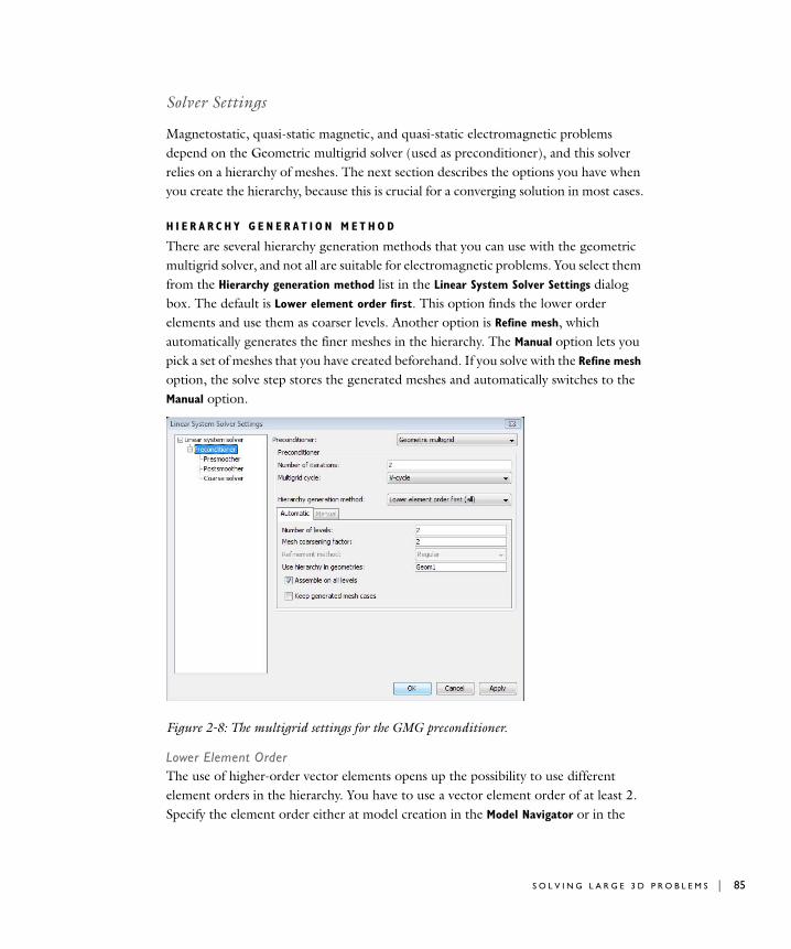
Solver Settings
Magnetostatic, quasi-static magnetic, and quasi-static electromagnetic problems depend on the Geometric multigrid solver (used as preconditioner), and this solver relies on a hierarchy of meshes. The next section describes the options you have when you create the hierarchy, because this is crucial for a converging solution in most cases.
H I E R A R C H Y G E N E R A T I O N M E T H O D
There are several hierarchy generation methods that you can use with the geometric multigrid solver, and not all are suitable for electromagnetic problems. You select them from the Hierarchy generation method list in the Linear System Solver Settings dialog box. The default is Lower element order first. This option finds the lower order elements and use them as coarser levels. Another option is Refine mesh, which automatically generates the finer meshes in the hierarchy. The Manual option lets you pick a set of meshes that you have created beforehand. If you solve with the Refine mesh option, the solve step stores the generated meshes and automatically switches to the Manual option.
Figure 2-8: The multigrid settings for the GMG preconditioner.
Lower Element OrderThe use of higher-order vector elements opens up the possibility to use different element orders in the hierarchy. You have to use a vector element order of at least 2. Specify the element order either at model creation in the Model Navigator or in the
S O L V I N G L A R G E 3 D P R O B L E M S | 85
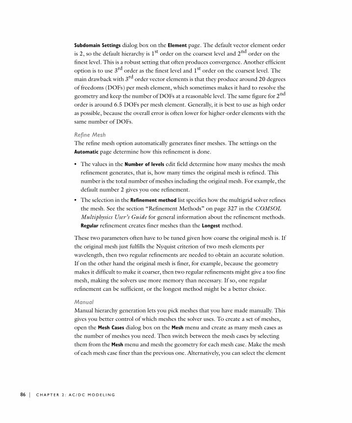
86 | C H A P T E R
Subdomain Settings dialog box on the Element page. The default vector element order is 2, so the default hierarchy is 1st order on the coarsest level and 2nd order on the finest level. This is a robust setting that often produces convergence. Another efficient option is to use 3rd order as the finest level and 1st order on the coarsest level. The main drawback with 3rd order vector elements is that they produce around 20 degrees of freedoms (DOFs) per mesh element, which sometimes makes it hard to resolve the geometry and keep the number of DOFs at a reasonable level. The same figure for 2nd order is around 6.5 DOFs per mesh element. Generally, it is best to use as high order as possible, because the overall error is often lower for higher-order elements with the same number of DOFs.
Refine MeshThe refine mesh option automatically generates finer meshes. The settings on the Automatic page determine how this refinement is done.
• The values in the Number of levels edit field determine how many meshes the mesh refinement generates, that is, how many times the original mesh is refined. This number is the total number of meshes including the original mesh. For example, the default number 2 gives you one refinement.
• The selection in the Refinement method list specifies how the multigrid solver refines the mesh. See the section “Refinement Methods” on page 327 in the COMSOL Multiphysics User’s Guide for general information about the refinement methods. Regular refinement creates finer meshes than the Longest method.
These two parameters often have to be tuned given how coarse the original mesh is. If the original mesh just fulfills the Nyquist criterion of two mesh elements per wavelength, then two regular refinements are needed to obtain an accurate solution. If on the other hand the original mesh is finer, for example, because the geometry makes it difficult to make it coarser, then two regular refinements might give a too fine mesh, making the solvers use more memory than necessary. If so, one regular refinement can be sufficient, or the longest method might be a better choice.
ManualManual hierarchy generation lets you pick meshes that you have made manually. This gives you better control of which meshes the solver uses. To create a set of meshes, open the Mesh Cases dialog box on the Mesh menu and create as many mesh cases as the number of meshes you need. Then switch between the mesh cases by selecting them from the Mesh menu and mesh the geometry for each mesh case. Make the mesh of each mesh case finer than the previous one. Alternatively, you can select the element
2 : A C / D C M O D E L I N G
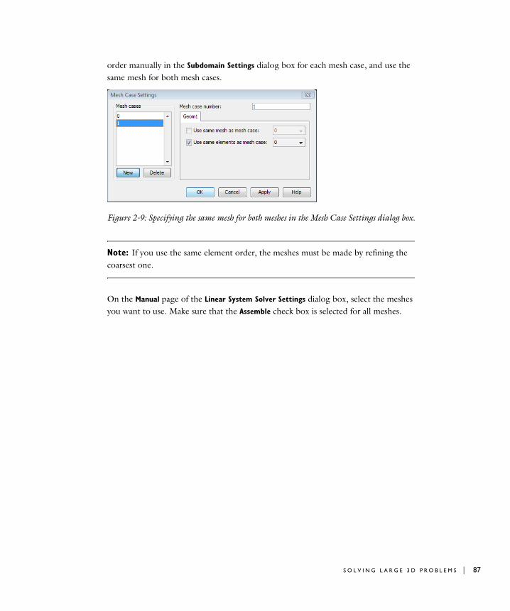
order manually in the Subdomain Settings dialog box for each mesh case, and use the same mesh for both mesh cases.
Figure 2-9: Specifying the same mesh for both meshes in the Mesh Case Settings dialog box.
Note: If you use the same element order, the meshes must be made by refining the coarsest one.
On the Manual page of the Linear System Solver Settings dialog box, select the meshes you want to use. Make sure that the Assemble check box is selected for all meshes.
S O L V I N G L A R G E 3 D P R O B L E M S | 87
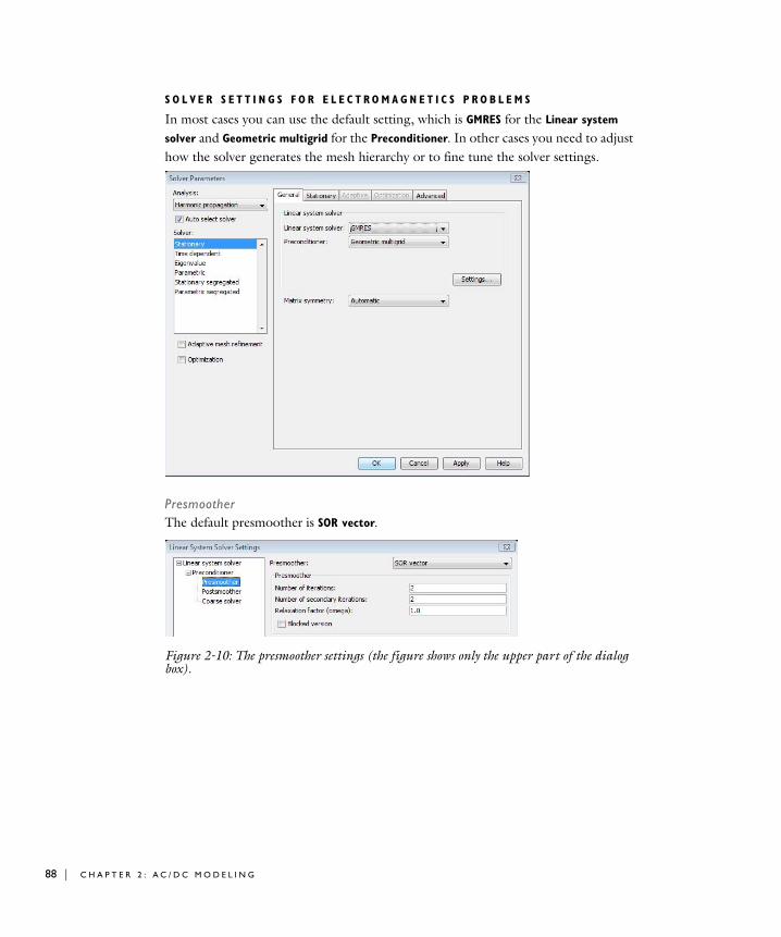
88 | C H A P T E R
S O L V E R S E T T I N G S F O R E L E C T R O M A G N E T I C S P R O B L E M S
In most cases you can use the default setting, which is GMRES for the Linear system
solver and Geometric multigrid for the Preconditioner. In other cases you need to adjust how the solver generates the mesh hierarchy or to fine tune the solver settings.
PresmootherThe default presmoother is SOR vector.
Figure 2-10: The presmoother settings (the figure shows only the upper part of the dialog box).
2 : A C / D C M O D E L I N G
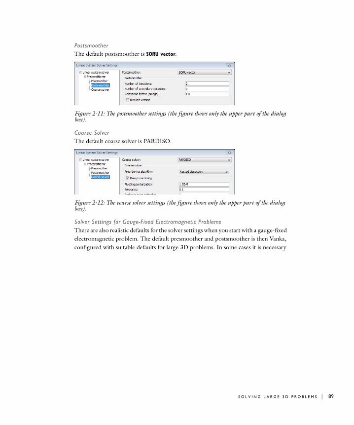
PostsmootherThe default postsmoother is SORU vector.
Figure 2-11: The postsmoother settings (the figure shows only the upper part of the dialog box).
Coarse SolverThe default coarse solver is PARDISO.
Figure 2-12: The coarse solver settings (the figure shows only the upper part of the dialog box).
Solver Settings for Gauge-Fixed Electromagnetic ProblemsThere are also realistic defaults for the solver settings when you start with a gauge-fixed electromagnetic problem. The default presmoother and postsmoother is then Vanka, configured with suitable defaults for large 3D problems. In some cases it is necessary
S O L V I N G L A R G E 3 D P R O B L E M S | 89
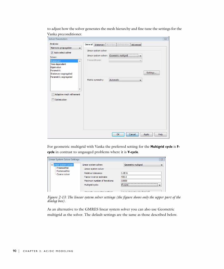
90 | C H A P T E R
to adjust how the solver generates the mesh hierarchy and fine tune the settings for the Vanka preconditioner.
For geometric multigrid with Vanka the preferred setting for the Multigrid cycle is F-cycle in contrast to ungauged problems where it is V-cycle.
Figure 2-13: The linear system solver settings (the figure shows only the upper part of the dialog box).
As an alternative to the GMRES linear system solver you can also use Geometric multigrid as the solver. The default settings are the same as those described below.
2 : A C / D C M O D E L I N G
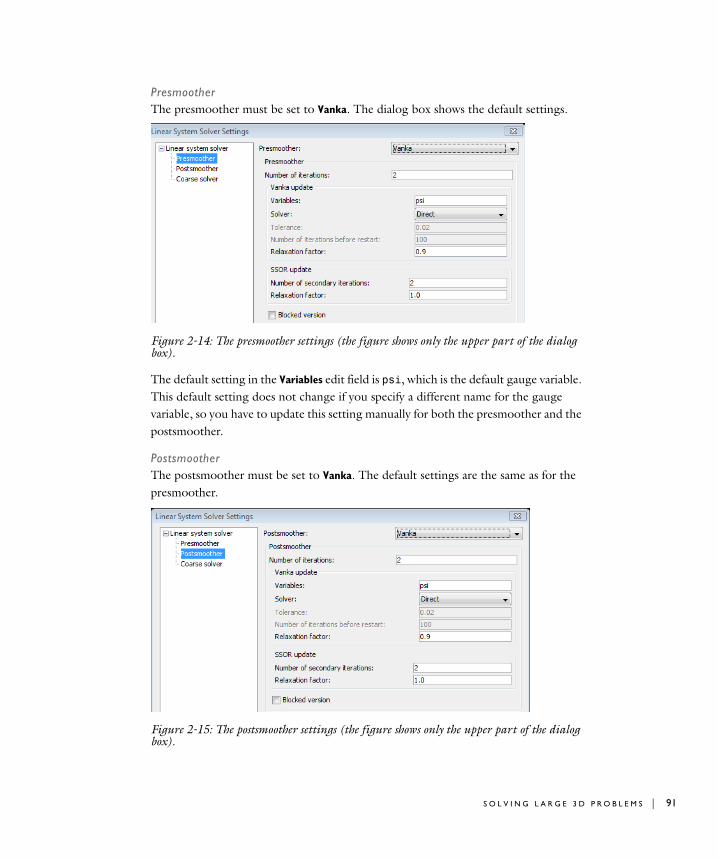
PresmootherThe presmoother must be set to Vanka. The dialog box shows the default settings.
Figure 2-14: The presmoother settings (the figure shows only the upper part of the dialog box).
The default setting in the Variables edit field is psi, which is the default gauge variable. This default setting does not change if you specify a different name for the gauge variable, so you have to update this setting manually for both the presmoother and the postsmoother.
PostsmootherThe postsmoother must be set to Vanka. The default settings are the same as for the presmoother.
Figure 2-15: The postsmoother settings (the figure shows only the upper part of the dialog box).
S O L V I N G L A R G E 3 D P R O B L E M S | 91
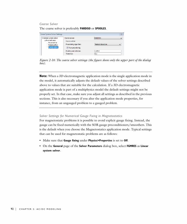
92 | C H A P T E R
Coarse SolverThe coarse solver is preferably PARDISO or SPOOLES.
Figure 2-16: The coarse solver settings (the figure shows only the upper part of the dialog box).
Note: When a 3D electromagnetic application mode is the single application mode in the model, it automatically adjusts the default values of the solver settings described above to values that are suitable for the calculation. If a 3D electromagnetic application mode is part of a multiphysics model the default settings might not be properly set. In that case, make sure you adjust all settings as described in the previous sections. This is also necessary if you alter the application mode properties, for instance, from an ungauged problem to a gauged problem.
Solver Settings for Numerical Gauge Fixing in MagnetostaticsFor magnetostatic problems it is possible to avoid explicit gauge fixing. Instead, the gauge can be fixed numerically with the SOR gauge preconditioners/smoothers. This is the default when you choose the Magnetostatics application mode. Typical settings that can be used for magnetostatic problems are as follows:
• Make sure that Gauge fixing under Physics>Properties is set to Off.
• On the General page of the Solver Parameters dialog box, select FGMRES as Linear
system solver.
2 : A C / D C M O D E L I N G
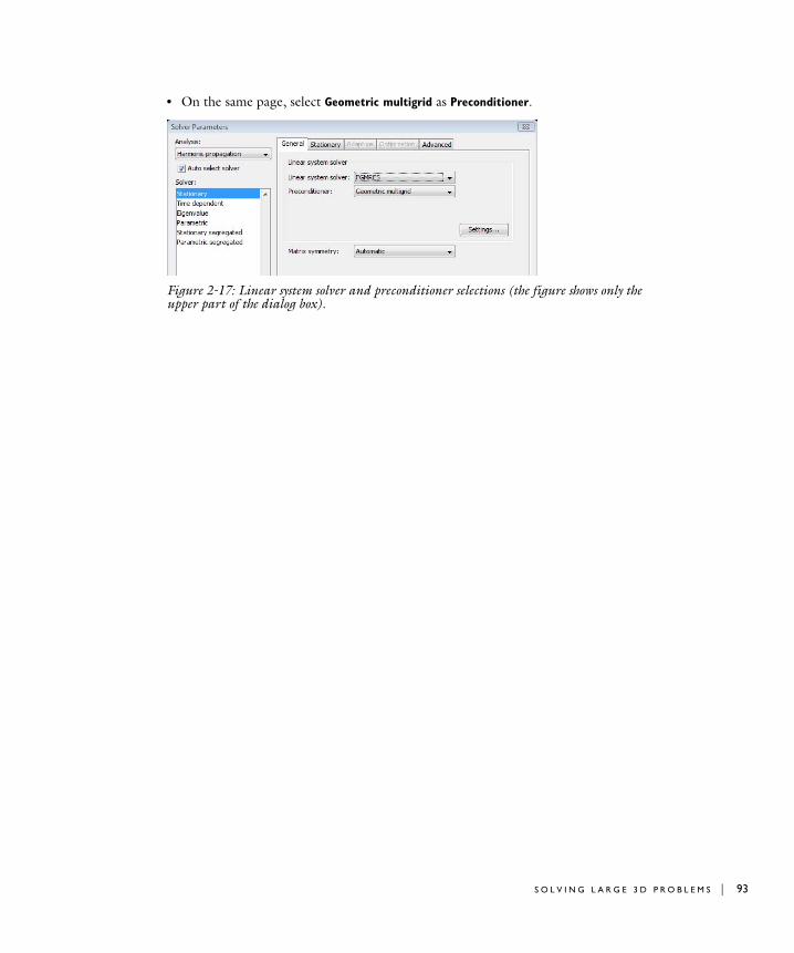
• On the same page, select Geometric multigrid as Preconditioner.
Figure 2-17: Linear system solver and preconditioner selections (the figure shows only the upper part of the dialog box).
S O L V I N G L A R G E 3 D P R O B L E M S | 93
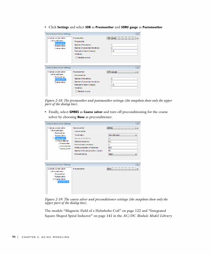
94 | C H A P T E R
• Click Settings and select SOR as Presmoother and SORU gauge as Postsmoother.
Figure 2-18: The presmoother and postsmoother settings (the snapshots show only the upper part of the dialog box).
• Finally, select GMRES as Coarse solver and turn off preconditioning for the coarse solver by choosing None as preconditioner.
Figure 2-19: The coarse solver and preconditioner settings (the snapshots show only the upper part of the dialog box).
The models “Magnetic Field of a Helmholtz Coil” on page 122 and “Integrated Square-Shaped Spiral Inductor” on page 141 in the AC/DC Module Model Library
2 : A C / D C M O D E L I N G
are examples where the described approach involving SOR gauge is used. In these two models the entire computational domain is treated as being magnetostatic. The models therefore include all vector degrees of freedom in the divergence cleaning performed by SORU gauge; see “The SSOR Gauge, SOR Gauge, and SORU Gauge Algorithms” on page 530 in the COMSOL Multiphysics Reference Guide. By default, all vector degrees of freedom are included in the divergence cleaning. Leaving the Variables edit field empty for the SORU gauge postsmoother therefore gives the same result for the two mentioned models as entering tAxAyAz10, tAxAyAz20, and tAxAyAz21 in that edit field.
Note: The SOR gauge smoothers remove any nondivergence-free parts of the right-hand side of the linear system of equations. For instance, the external current density, Je, appears in the right-hand side. Nondivergence-free components of Je are consequently removed.
Solver Settings for Ungauged FormulationsIn some situations it is possible to solve a problem without any gauge fixing. The models “Magnetic Brake in 3D” on page 72 and “Railgun” on page 84 of the AC/DC Module Model Library use these special ungauged formulations. There are also separate entries for 3D models in the Model Navigator that have these settings as default, for example, Quasi-Statics, Electromagnetic>Electric and Induction Currents>
Time-harmonic analysis, ungauged AV.
The Mesh Cases After Solving
When you have solved using automatic generation of the mesh hierarchy using the Refine mesh method, you can find the meshes as mesh cases on the Mesh menu. The finest mesh is the one that the solver used to calculate the final solution, and it shows how well the geometry has been resolved.
When you have solved using the refine mesh hierarchy, the Hierarchy generation method in the Linear Solver Settings dialog box switches to Manual. This means that if you solve again, the solver uses the same meshes.
If you want to use the refine mesh generation again but with different refinement parameters or another coarse mesh, you must change the Hierarchy generation method back to Refine mesh. The solver then generates another set of meshes. In the Mesh Cases
S O L V I N G L A R G E 3 D P R O B L E M S | 95

96 | C H A P T E R
dialog box, you can delete the additional meshes that were used for the previous solution but are no longer used.
If you solve using the Lower element order first method, the solver generates the hierarchy on the current mesh each time you solve, so you do not have to adjust any solver parameters.
2 : A C / D C M O D E L I N G
U s i n g A s s emb l i e s i n E l e c t r omagne t i c s P r ob l em s
The use of assemblies in models can simplify and improve several aspects of modeling. For electromagnetics applications you can use it to make devices move and rotate with the sliding mesh technique. The model “Generator” in the AC/DC Module Model Library is an example that uses this technique. Another situation when assemblies come in handy is when you need to introduce a discontinuity for the solution variable at an interface. Such interface conditions are generally called slit boundary conditions. For example, a distributed impedance between two conducting layers that creates a voltage difference between the two layers. The sliding mesh interface can also be seen as a slit boundary. A third example of assembly usage is when you want to mix mesh element types and mesh resolution, because you can mesh the two neighboring parts of the assembly independently. You can mix element without using assemblies as long as the boundary mesh elements at an interface are the same. This is true for interfaces between quadrilateral and triangular elements in 2D, and tetrahedral elements facing the triangular bases of prism elements in 3D.
Although assemblies simplifies several task in modeling, there are a few important rules and recommendations that need consideration, and these are covered in the following sections.
Assemblies and Vector Elements
If you use an application mode with vector elements it might be necessary to activate gauge fixing. This is the same type of gauge fixing that you need when solving magnetostatics problems. The property value Automatic in the Gauge fixing list automatically turns on gauge fixing if the model has assemblies with pairs. The only situation where you can turn the gauge fixing off is when the boundary meshes on each side of the assembly interface are identical.
For 2D problems, for which you can use direct solvers, activating gauge fixing usually does not cause any trouble. It is when you solve 3D problems with iterative solvers that you need to know wether the gauge fixing is activated or not. When gauge fixing is activated there is an extra solution variable, psi, added to the problem that needs the Vanka preconditioner/solver with psi as Vanka variable. You can find details about
U S I N G A S S E M B L I E S I N E L E C T R O M A G N E T I C S P R O B L E M S | 97
98 | C H A P T E R
these solver settings in “Solver Settings for Gauge-Fixed Electromagnetic Problems” on page 89.
The application modes in the AC/DC Module that use vector elements all solve for the magnetic vector potential, A.
Note: The property value Automatic in the Gauge fixing list also detects if the application mode needs gauge fixing even without assemblies. It does not detect whether the meshes at the interface are identical. In that case you must manually select Off in the Gauge fixing list.
Generally, avoid activating gauge fixing if it is possible. The problem is much tougher to solve when it is activated in terms of solution time and memory usage. There are techniques to create compatible (or identical) meshes, and these are briefly described below.
C O M P A T I B L E M E S H E S
Use interactive meshing and mesh only the source or destination side of pair boundaries first. Then select both source and destination boundaries and click the Copy
Mesh button on the Mesh toolbar. You can read more about the copy mesh feature in “Copying Meshes” on page 342 in the COMSOL Multiphysics User’s Guide.
Note: For a sliding mesh interface it is not possible to generate compatible meshes. A mesh that is compatible at a one time is probably not compatible at a later time when the destination side has moved slightly.
Assemblies and Weak Constraints
It might be necessary to use weak constraints to improve the accuracy at the assembly interface. Especially when the interface is a sliding mesh interface. Weak constraints also add extra complexity for the settings of the iterative solvers, so it might not be
2 : A C / D C M O D E L I N G
possible to use them for large 3D problems. Below are a few recommendations when to use and how to use weak constraints for assemblies:
• If you have a transient problem with a moving assembly interface that fails to converge after some time, you might get better convergence if you turn on weak constraints.
• The recommendation is generally to mesh the destination boundary finer than the source boundary, but it is not as crucial when you use weak constraints compared to pointwise constraints.
When you turn on weak constraints, it is activated for all boundaries with constraints on the solution variable, and for all boundaries with coupling through assembly pairs (for example, identity pairs). The difference in magnitude of the Lagrange multiplier between the assembly pairs and other constraints may be several orders of magnitude, which can cause convergence problems and even a singular matrix error. If you get such problems, it is recommended to deactivate the weak constraints manually for all other constraints except the assembly pair boundaries. You do this by clearing the Use
weak constraints check box on the Weak Constr. page in the Boundary Settings dialog box.
U S I N G A S S E M B L I E S I N E L E C T R O M A G N E T I C S P R O B L E M S | 99

100 | C H A P T E R
2 : A C / D C M O D E L I N G
3
R e v i e w o f E l e c t r o m a g n e t i c s
This chapter contains an overview of the theory behind the AC/DC Module. It is intended for readers that wish to understand what goes on behind the scenes.
101
102 | C H A P T E R
Maxwe l l ’ s Equa t i o n s
The problem of electromagnetic analysis on a macroscopic level is the problem of solving Maxwell’s equations subject to certain boundary conditions. Maxwell’s equations are a set of equations, written in differential or integral form, stating the relationships between the fundamental electromagnetic quantities. These quantities are the electric field intensity E, the electric displacement or electric flux density D, the magnetic field intensity H, the magnetic flux density B, the current density J, and the electric charge density ρ.
The equations can be formulated in differential or integral form. The differential form is presented here, because it leads to differential equations that the finite element method can handle. For general time-varying fields, Maxwell’s equations can be written as
The first two equations are also referred to as Maxwell-Ampère’s law and Faraday’s law, respectively. Equation three and four are two forms of Gauss’ law—the electric and magnetic form, respectively.
Another fundamental equation is the equation of continuity, which can be written as
Out of the five equations mentioned, only three are independent. The first two combined with either the electric form of Gauss’ law or the equation of continuity form such an independent system.
Constitutive Relations
To obtain a closed system, the equations include constitutive relations that describe the macroscopic properties of the medium. They are given as
∇ H× J D∂t∂
-------+=
∇ E× B∂t∂
-------–=
∇ D⋅ ρ=
∇ B⋅ 0=
∇ J⋅ ρ∂t∂
------–=
3 : R E V I E W O F E L E C T R O M A G N E T I C S
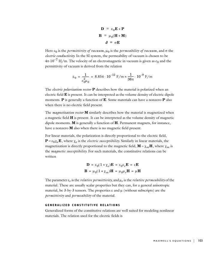
Here ε0 is the permittivity of vacuum, µ0 is the permeability of vacuum, and σ the electric conductivity. In the SI system, the permeability of vacuum is chosen to be 4π·10−7 H/m. The velocity of an electromagnetic in vacuum is given as c0 and the permittivity of vacuum is derived from the relation
The electric polarization vector P describes how the material is polarized when an electric field E is present. It can be interpreted as the volume density of electric dipole moments. P is generally a function of E. Some materials can have a nonzero P also when there is no electric field present.
The magnetization vector M similarly describes how the material is magnetized when a magnetic field H is present. It can be interpreted as the volume density of magnetic dipole moments. M is generally a function of H. Permanent magnets, for instance, have a nonzero M also when there is no magnetic field present.
For linear materials, the polarization is directly proportional to the electric field, P = ε0 χe E , where χe is the electric susceptibility. Similarly in linear materials, the magnetization is directly proportional to the magnetic field, M = χm H , where χm is the magnetic susceptibility. For such materials, the constitutive relations can be written
The parameter εr is the relative permittivity, and µr is the relative permeability of the material. These are usually scalar properties but they can, for a general anisotropic material, be 3-by-3 tensors. The properties ε and µ (without subscripts) are the permittivity and permeability of the material.
G E N E R A L I Z E D C O N S T I T U T I V E R E L A T I O N S
Generalized forms of the constitutive relations are well suited for modeling nonlinear materials. The relation used for the electric fields is
D ε0E P+=B µ0 H M+( )=
J σE=
ε01
c02µ0
---------- 8.854 10 12– F/m 136π--------- 10 9– F/m⋅≈⋅= =
D ε0 1 χe+( )E ε0εrE εE= = =
B µ0 1 χm+( )H µ0µrH µH= = =
M A X W E L L ’ S E Q U A T I O N S | 103
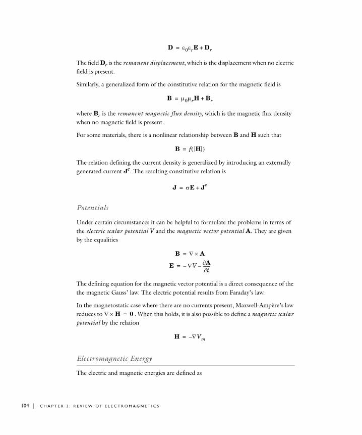
104 | C H A P T E R
The field Dr is the remanent displacement, which is the displacement when no electric field is present.
Similarly, a generalized form of the constitutive relation for the magnetic field is
where Br is the remanent magnetic flux density, which is the magnetic flux density when no magnetic field is present.
For some materials, there is a nonlinear relationship between B and H such that
The relation defining the current density is generalized by introducing an externally generated current Je. The resulting constitutive relation is
Potentials
Under certain circumstances it can be helpful to formulate the problems in terms of the electric scalar potential V and the magnetic vector potential A. They are given by the equalities
The defining equation for the magnetic vector potential is a direct consequence of the the magnetic Gauss’ law. The electric potential results from Faraday’s law.
In the magnetostatic case where there are no currents present, Maxwell-Ampère’s law reduces to . When this holds, it is also possible to define a magnetic scalar potential by the relation
Electromagnetic Energy
The electric and magnetic energies are defined as
D ε0εrE Dr+=
B µ0µrH Br+=
B f H( )=
J σE Je+=
B ∇ A×=
E ∇V– A∂t∂
-------–=
∇ H× 0=
H ∇Vm–=
3 : R E V I E W O F E L E C T R O M A G N E T I C S
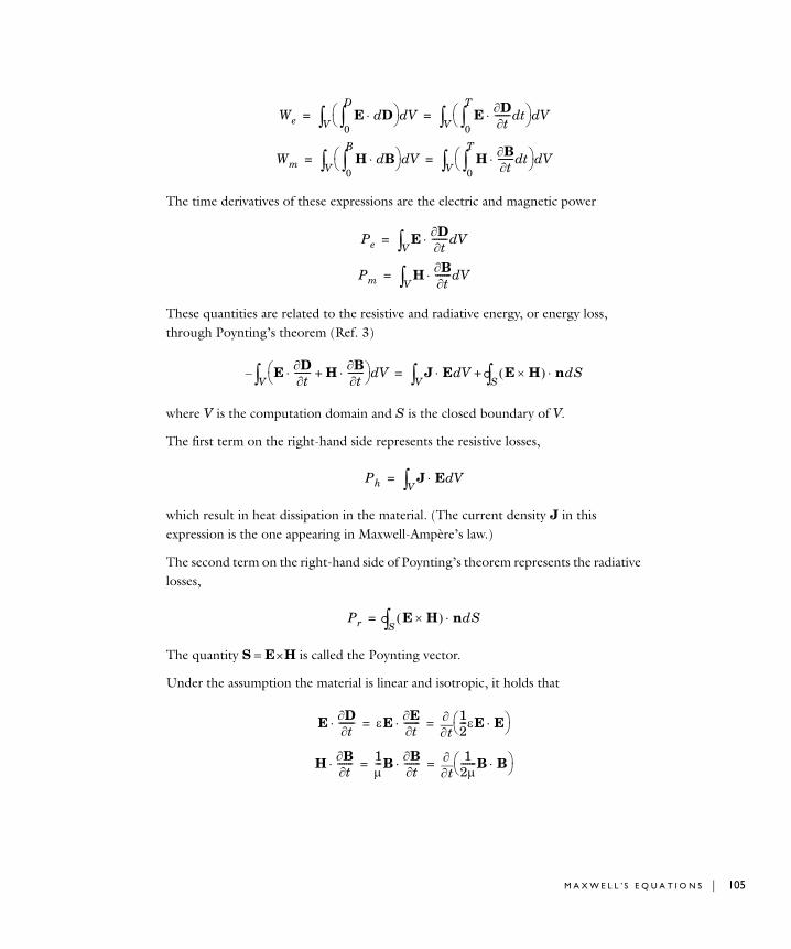
The time derivatives of these expressions are the electric and magnetic power
These quantities are related to the resistive and radiative energy, or energy loss, through Poynting’s theorem (Ref. 3)
where V is the computation domain and S is the closed boundary of V.
The first term on the right-hand side represents the resistive losses,
which result in heat dissipation in the material. (The current density J in this expression is the one appearing in Maxwell-Ampère’s law.)
The second term on the right-hand side of Poynting’s theorem represents the radiative losses,
The quantity S = E × H is called the Poynting vector.
Under the assumption the material is linear and isotropic, it holds that
We E Dd⋅0
D
∫⎝ ⎠⎛ ⎞ Vd
V∫ E D∂t∂
-------⋅ td0
T
∫⎝ ⎠⎛ ⎞ Vd
V∫= =
Wm H Bd⋅0
B
∫⎝ ⎠⎛ ⎞ Vd
V∫ H B∂t∂
-------⋅ td0
T
∫⎝ ⎠⎛ ⎞ Vd
V∫= =
Pe E D∂t∂
-------⋅ VdV∫=
Pm H B∂t∂
-------⋅ VdV∫=
E D∂t∂
-------⋅ H B∂t∂
-------⋅+⎝ ⎠⎛ ⎞ Vd
V∫– J E⋅ VdV∫ E H×( ) n⋅ dS
S∫°+=
Ph J E⋅ VdV∫=
Pr E H×( ) n⋅ dSS∫°=
E D∂t∂
-------⋅ εE E∂t∂
-------⋅t∂
∂ 12---εE E⋅⎝ ⎠
⎛ ⎞= =
H B∂t∂
-------⋅ 1µ---B B∂
t∂-------⋅
t∂∂ 1
2µ-------B B⋅⎝ ⎠
⎛ ⎞= =
M A X W E L L ’ S E Q U A T I O N S | 105
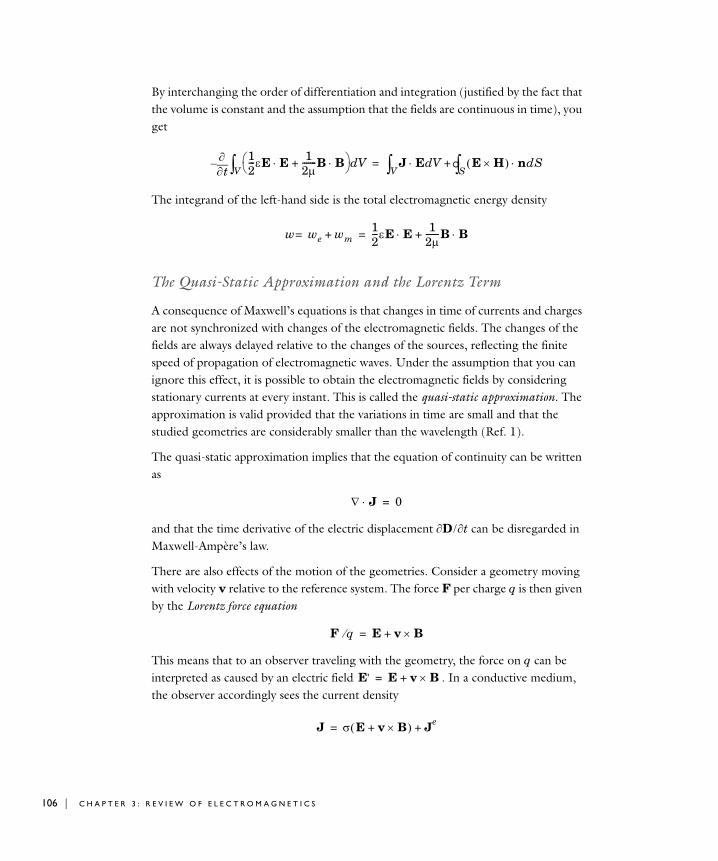
106 | C H A P T E R
By interchanging the order of differentiation and integration (justified by the fact that the volume is constant and the assumption that the fields are continuous in time), you get
The integrand of the left-hand side is the total electromagnetic energy density
The Quasi-Static Approximation and the Lorentz Term
A consequence of Maxwell’s equations is that changes in time of currents and charges are not synchronized with changes of the electromagnetic fields. The changes of the fields are always delayed relative to the changes of the sources, reflecting the finite speed of propagation of electromagnetic waves. Under the assumption that you can ignore this effect, it is possible to obtain the electromagnetic fields by considering stationary currents at every instant. This is called the quasi-static approximation. The approximation is valid provided that the variations in time are small and that the studied geometries are considerably smaller than the wavelength (Ref. 1).
The quasi-static approximation implies that the equation of continuity can be written as
and that the time derivative of the electric displacement ∂D / ∂t can be disregarded in Maxwell-Ampère’s law.
There are also effects of the motion of the geometries. Consider a geometry moving with velocity v relative to the reference system. The force F per charge q is then given by the Lorentz force equation
This means that to an observer traveling with the geometry, the force on q can be interpreted as caused by an electric field . In a conductive medium, the observer accordingly sees the current density
t∂∂ 1
2---εE E⋅ 1
2µ-------B B⋅+⎝ ⎠
⎛ ⎞ VdV∫– J E⋅ Vd
V∫ E H×( ) n⋅ dSS∫°+=
w we wm+=12---εE E⋅ 1
2µ-------B B⋅+=
∇ J⋅ 0=
F q⁄ E v B×+=
E' E v B×+=
J σ E v B×+( ) Je+=
3 : R E V I E W O F E L E C T R O M A G N E T I C S
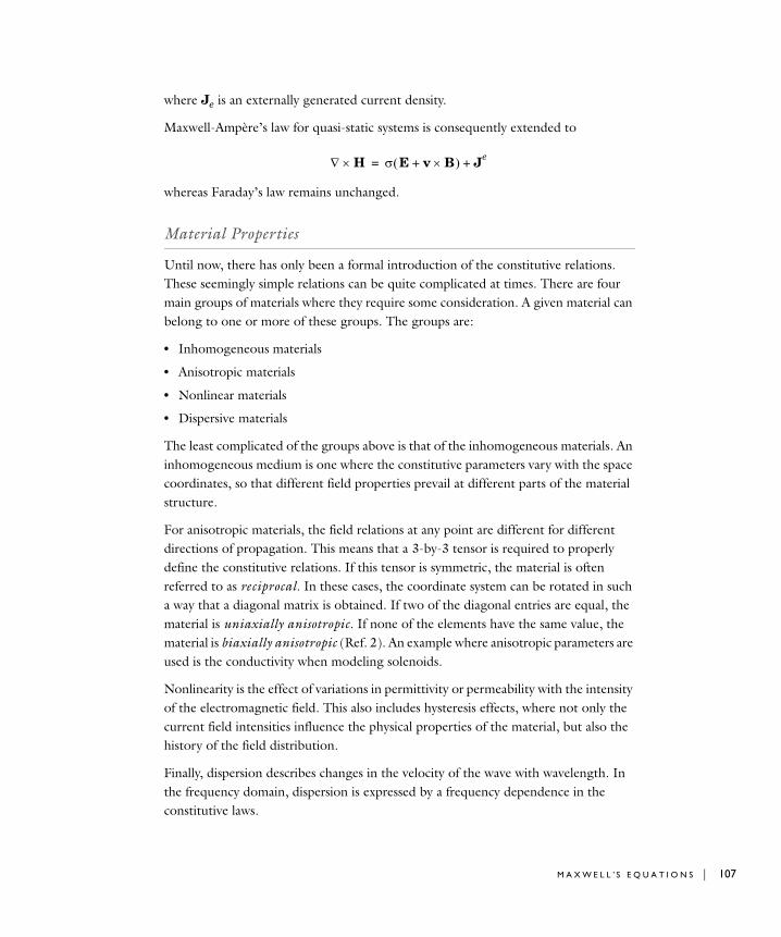
where Je is an externally generated current density.
Maxwell-Ampère’s law for quasi-static systems is consequently extended to
whereas Faraday’s law remains unchanged.
Material Properties
Until now, there has only been a formal introduction of the constitutive relations. These seemingly simple relations can be quite complicated at times. There are four main groups of materials where they require some consideration. A given material can belong to one or more of these groups. The groups are:
• Inhomogeneous materials
• Anisotropic materials
• Nonlinear materials
• Dispersive materials
The least complicated of the groups above is that of the inhomogeneous materials. An inhomogeneous medium is one where the constitutive parameters vary with the space coordinates, so that different field properties prevail at different parts of the material structure.
For anisotropic materials, the field relations at any point are different for different directions of propagation. This means that a 3-by-3 tensor is required to properly define the constitutive relations. If this tensor is symmetric, the material is often referred to as reciprocal. In these cases, the coordinate system can be rotated in such a way that a diagonal matrix is obtained. If two of the diagonal entries are equal, the material is uniaxially anisotropic. If none of the elements have the same value, the material is biaxially anisotropic (Ref. 2). An example where anisotropic parameters are used is the conductivity when modeling solenoids.
Nonlinearity is the effect of variations in permittivity or permeability with the intensity of the electromagnetic field. This also includes hysteresis effects, where not only the current field intensities influence the physical properties of the material, but also the history of the field distribution.
Finally, dispersion describes changes in the velocity of the wave with wavelength. In the frequency domain, dispersion is expressed by a frequency dependence in the constitutive laws.
∇ H× σ E v B×+( ) Je+=
M A X W E L L ’ S E Q U A T I O N S | 107
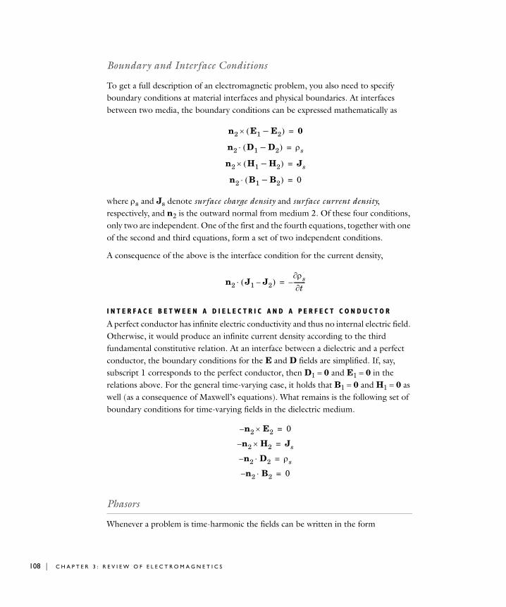
108 | C H A P T E R
Boundary and Interface Conditions
To get a full description of an electromagnetic problem, you also need to specify boundary conditions at material interfaces and physical boundaries. At interfaces between two media, the boundary conditions can be expressed mathematically as
where ρs and Js denote surface charge density and surface current density, respectively, and n2 is the outward normal from medium 2. Of these four conditions, only two are independent. One of the first and the fourth equations, together with one of the second and third equations, form a set of two independent conditions.
A consequence of the above is the interface condition for the current density,
I N T E R F A C E B E T W E E N A D I E L E C T R I C A N D A P E R F E C T C O N D U C T O R
A perfect conductor has infinite electric conductivity and thus no internal electric field. Otherwise, it would produce an infinite current density according to the third fundamental constitutive relation. At an interface between a dielectric and a perfect conductor, the boundary conditions for the E and D fields are simplified. If, say, subscript 1 corresponds to the perfect conductor, then D1 = 0 and E1 = 0 in the relations above. For the general time-varying case, it holds that B1 = 0 and H1 = 0 as well (as a consequence of Maxwell’s equations). What remains is the following set of boundary conditions for time-varying fields in the dielectric medium.
Phasors
Whenever a problem is time-harmonic the fields can be written in the form
n2 E1 E2–( )× 0=
n2 D1 D2–( )⋅ ρs=
n2 H1 H2–( )× Js=
n2 B1 B2–( )⋅ 0=
n2 J1 J2–( )⋅ρs∂t∂
--------–=
n– 2 E2× 0=
n– 2 H2× Js=
n– 2 D2⋅ ρs=
n– 2 B2⋅ 0=
3 : R E V I E W O F E L E C T R O M A G N E T I C S
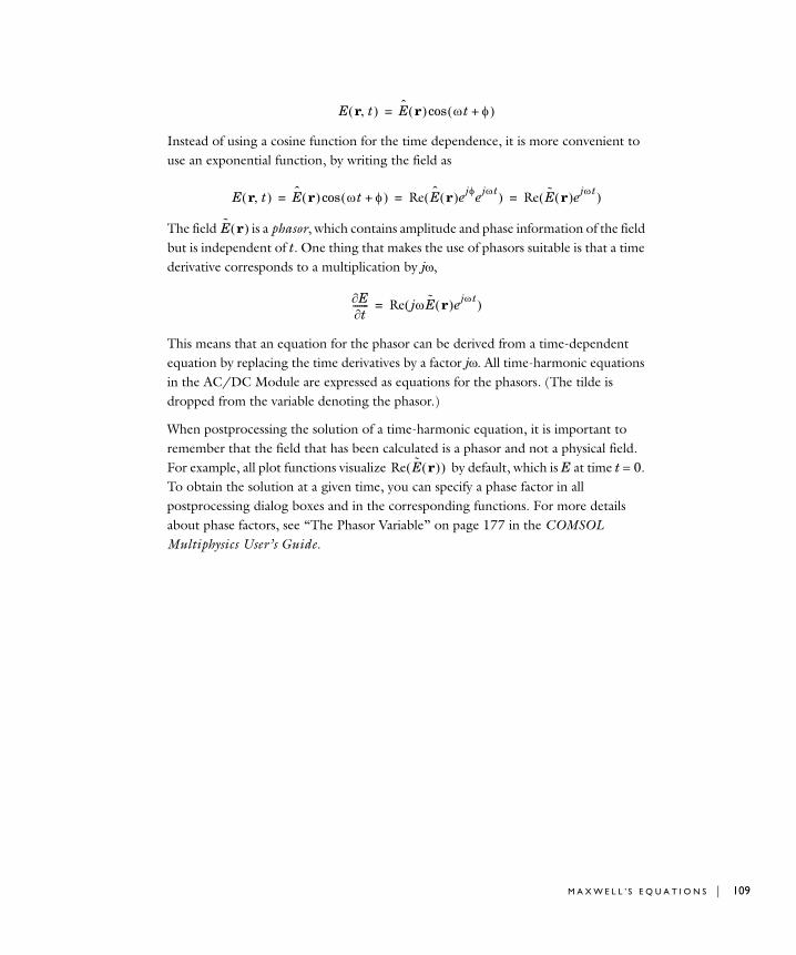
Instead of using a cosine function for the time dependence, it is more convenient to use an exponential function, by writing the field as
The field is a phasor, which contains amplitude and phase information of the field but is independent of t. One thing that makes the use of phasors suitable is that a time derivative corresponds to a multiplication by jω,
This means that an equation for the phasor can be derived from a time-dependent equation by replacing the time derivatives by a factor jω. All time-harmonic equations in the AC/DC Module are expressed as equations for the phasors. (The tilde is dropped from the variable denoting the phasor.)
When postprocessing the solution of a time-harmonic equation, it is important to remember that the field that has been calculated is a phasor and not a physical field. For example, all plot functions visualize by default, which is E at time t = 0. To obtain the solution at a given time, you can specify a phase factor in all postprocessing dialog boxes and in the corresponding functions. For more details about phase factors, see “The Phasor Variable” on page 177 in the COMSOL Multiphysics User’s Guide.
E r t,( ) E r( ) ωt φ+( )cos=
E r t,( ) E r( ) ωt φ+( )cos Re E r( )ejφejωt( ) Re E r( )ejωt( )= = =
E r( )
E∂t∂
------- Re jωE r( )ejωt( )=
Re E r( )( )
M A X W E L L ’ S E Q U A T I O N S | 109
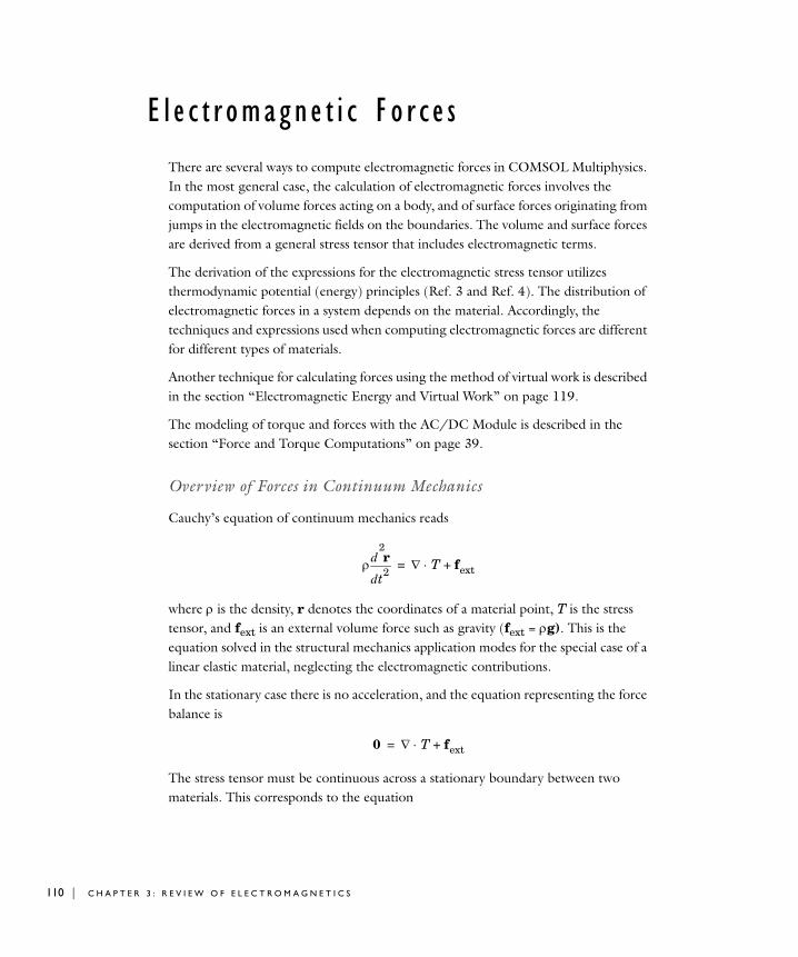
110 | C H A P T E R
E l e c t r omagne t i c F o r c e s
There are several ways to compute electromagnetic forces in COMSOL Multiphysics. In the most general case, the calculation of electromagnetic forces involves the computation of volume forces acting on a body, and of surface forces originating from jumps in the electromagnetic fields on the boundaries. The volume and surface forces are derived from a general stress tensor that includes electromagnetic terms.
The derivation of the expressions for the electromagnetic stress tensor utilizes thermodynamic potential (energy) principles (Ref. 3 and Ref. 4). The distribution of electromagnetic forces in a system depends on the material. Accordingly, the techniques and expressions used when computing electromagnetic forces are different for different types of materials.
Another technique for calculating forces using the method of virtual work is described in the section “Electromagnetic Energy and Virtual Work” on page 119.
The modeling of torque and forces with the AC/DC Module is described in the section “Force and Torque Computations” on page 39.
Overview of Forces in Continuum Mechanics
Cauchy’s equation of continuum mechanics reads
where ρ is the density, r denotes the coordinates of a material point, T is the stress tensor, and fext is an external volume force such as gravity (fext = ρg). This is the equation solved in the structural mechanics application modes for the special case of a linear elastic material, neglecting the electromagnetic contributions.
In the stationary case there is no acceleration, and the equation representing the force balance is
The stress tensor must be continuous across a stationary boundary between two materials. This corresponds to the equation
ρt2
2
d
d r ∇ T fext+⋅=
0 ∇ T fext+⋅=
3 : R E V I E W O F E L E C T R O M A G N E T I C S
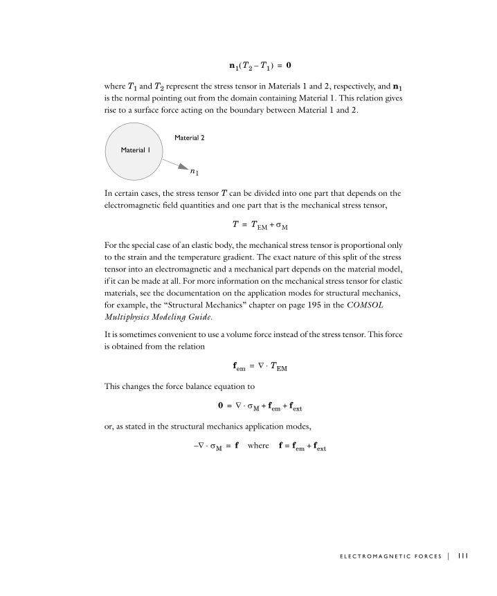
where T1 and T2 represent the stress tensor in Materials 1 and 2, respectively, and n1 is the normal pointing out from the domain containing Material 1. This relation gives rise to a surface force acting on the boundary between Material 1 and 2.
In certain cases, the stress tensor T can be divided into one part that depends on the electromagnetic field quantities and one part that is the mechanical stress tensor,
For the special case of an elastic body, the mechanical stress tensor is proportional only to the strain and the temperature gradient. The exact nature of this split of the stress tensor into an electromagnetic and a mechanical part depends on the material model, if it can be made at all. For more information on the mechanical stress tensor for elastic materials, see the documentation on the application modes for structural mechanics, for example, the “Structural Mechanics” chapter on page 195 in the COMSOL Multiphysics Modeling Guide.
It is sometimes convenient to use a volume force instead of the stress tensor. This force is obtained from the relation
This changes the force balance equation to
or, as stated in the structural mechanics application modes,
n1 T2 T1–( ) 0=
Material 1
Material 2
n1
T TEM σM+=
fem ∇ TEM⋅=
0 ∇ σM⋅ fem fext+ +=
∇– σM⋅ f where f fem fext+==
E L E C T R O M A G N E T I C F O R C E S | 111
112 | C H A P T E R
Forces on an Elastic Solid Surrounded by Vacuum or Air
Consider now a solid (Material 1) surrounded by vacuum (Material 2). It is natural to associate the surface force on the boundary between the materials with the solid. Note that in many applications air can be approximated by vacuum.
In practice, the equation for the force balance also needs to include an external boundary force gext. It is nonzero on those parts of the boundary where it is necessary to compensate for the contributions to the stress tensor that you are not interested in or do not have enough information on. These contributions come from the influence of the adjacent domains. By approximating the surroundings by vacuum or air, the influence of these boundaries and their adjacent domains (that are not part of our model) on the electromagnetic fields are neglected.
On the boundary, the following equations apply:
The external boundary force gext can represent the reaction force from another body that the solid is attached to.
The equations for the balance of forces on the solid now become
For computing the total force F on the solid these equations need to be integrated over the entire solid and the solid/vacuum boundary
Now, according to Gauss’ theorem
This means that the external force
n1 T2 T1–( ) 0=
n1T2 n1T2 gext+=
∇ T1 fext+⋅ 0=
n1 T2 T1–( ) gext+ 0=
∇ T1 fext+⋅( ) VdΩ1
∫ n1 T2 T1–( ) gext+( ) SdΩ1∂∫°+ 0=
∇ T1⋅ VdΩ1
∫ n1T1 SdΩ1∂∫°– 0=
3 : R E V I E W O F E L E C T R O M A G N E T I C S
is needed to balance the term for the boundary integral of the stress tensor in the surrounding vacuum
to keep the solid stationary. That is
If the external forces are suddenly removed, the solid is no longer stationary, but F causes the solid to begin to move with an initial acceleration according to
where m is the total mass and a is the acceleration of the solid.
To summarize, the total force, F, is computed as a boundary integral of the stress tensor in vacuum on the outside of the solid. Note that to obtain this result, the contribution from the air pressure gradient has been neglected. This is equivalent of assuming that . A more detailed treatment shows that the pressure gradient contributes with a lifting (buoyancy) force on the solid.
Torque
The torque in the case of the previous section is given by
where rO is a point on the axis of rotation. This follows from a derivation similar to the one made for forces.
Forces in Stationary Fields
The electromagnetic fields are stationary if
Fext fext VdΩ1
∫ gext SdΩ1∂∫°+=
F n1T2 SdΩ1∂∫°=
Fext F+ 0=
ma ρd2r
dt2--------- Vd
Ω1
∫ F= =
∇ T2⋅ 0=
MO r rO–( ) n1T2( )× SdΩ1∂∫°=
E L E C T R O M A G N E T I C F O R C E S | 113
114 | C H A P T E R
that is, if the fields vary so slowly that you can neglect the contributions from induced currents and displacement currents.
Also assume that the objects modeled are not moving
so that there is no contributions from Lorentz forces. These are treated later on.
T H E E L E C T R O M A G N E T I C S T R E S S TE N S O R
The expressions for the stress tensor in a general electromagnetic context stems from a fusion of material theory, thermodynamics, continuum mechanics, and electromagnetic field theory. With the introduction of thermodynamic potentials for mechanical, thermal, and electromagnetic effects, explicit expressions for the stress tensor can be derived in a convenient way by forming the formal derivatives with respect to the different physical fields (Ref. 3 and Ref. 4). Alternative derivations can be made for vacuum (Ref. 5) but these cannot easily be generalized to polarized and magnetized materials.
Air and VacuumFor air, the stress tensor is
where p is the air pressure, I is the identity 3x3 tensor (or matrix), and E and B are 3x1 vectors. In this expression of the stress tensor, air is considered to be nonpolarizable and nonmagnetizable. When air is approximated by vacuum, p = 0. This expression, with p = 0, of the stress tensor is also known as the Maxwell stress tensor.
Using the fact that, for air, D = ε0E and B = µ0H the expression for the stress tensor can be written as
t∂∂B 0=
t∂∂D 0=
v 0=
T2 pI–ε02-----E E 1
2µ0---------B B⋅+⋅⎝ ⎠
⎛ ⎞ I– ε0EET 1µ0------BBT
+ +=
T2 pI–12---E D 1
2---H B⋅+⋅⎝ ⎠
⎛ ⎞ I– EDT HBT+ +=
3 : R E V I E W O F E L E C T R O M A G N E T I C S
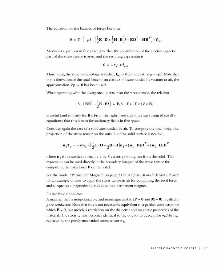
The equation for the balance of forces becomes
Maxwell’s equations in free space give that the contribution of the electromagnetic part of the stress tensor is zero, and the resulting expression is
Thus, using the same terminology as earlier, fem = 0 for air, with σM = −pI. Note that in the derivation of the total force on an elastic solid surrounded by vacuum or air, the approximation has been used.
When operating with the divergence operator on the stress tensor, the relation
is useful (and similarly for B). From the right-hand side it is clear (using Maxwell’s equations) that this is zero for stationary fields in free space.
Consider again the case of a solid surrounded by air. To compute the total force, the projection of the stress tensor on the outside of the solid surface is needed,
where n1 is the surface normal, a 1-by-3 vector, pointing out from the solid. This expression can be used directly in the boundary integral of the stress tensor for computing the total force F on the solid.
See the model “Permanent Magnet” on page 21 in AC/DC Module Model Library for an example of how to apply the stress tensor in air for computing the total force and torque on a magnetizable rod close to a permanent magnet.
Elastic Pure ConductorA material that is nonpolarizable and nonmagnetizable (P = 0 and M = 0) is called a pure conductor. Note that this is not necessarily equivalent to a perfect conductor, for which E = 0, but merely a restriction on the dielectric and magnetic properties of the material. The stress tensor becomes identical to the one for air, except for −pI being replaced by the purely mechanical stress tensor σM
0 ∇ pI–12---E D 1
2---H B⋅+⋅⎝ ⎠
⎛ ⎞ I– EDT HBT+ +⎝ ⎠
⎛ ⎞ fext+⋅=
0 p∇– fext+=
p∇ 0=
∇ EET 12---E EI⋅–⎝ ⎠
⎛ ⎞⋅ E ∇ E⋅( ) E ∇ E×( )×–=
n1T2 pn1–12---E D 1
2---H B⋅+⋅⎝ ⎠
⎛ ⎞ n1– n1 E⋅( )DT n1 H⋅( )BT+ +=
E L E C T R O M A G N E T I C F O R C E S | 115
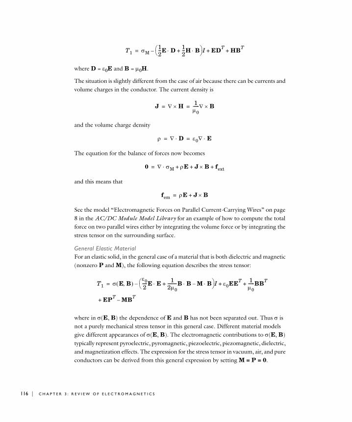
116 | C H A P T E R
where D = ε0E and B = µ0H.
The situation is slightly different from the case of air because there can be currents and volume charges in the conductor. The current density is
and the volume charge density
The equation for the balance of forces now becomes
and this means that
See the model “Electromagnetic Forces on Parallel Current-Carrying Wires” on page 8 in the AC/DC Module Model Library for an example of how to compute the total force on two parallel wires either by integrating the volume force or by integrating the stress tensor on the surrounding surface.
General Elastic MaterialFor an elastic solid, in the general case of a material that is both dielectric and magnetic (nonzero P and M), the following equation describes the stress tensor:
where in σ(E, B) the dependence of E and B has not been separated out. Thus σ is not a purely mechanical stress tensor in this general case. Different material models give different appearances of σ(E, B). The electromagnetic contributions to σ(E, B) typically represent pyroelectric, pyromagnetic, piezoelectric, piezomagnetic, dielectric, and magnetization effects. The expression for the stress tensor in vacuum, air, and pure conductors can be derived from this general expression by setting M = P = 0.
T1 σM12---E D 1
2---H B⋅+⋅⎝ ⎠
⎛ ⎞ I– EDT HBT+ +=
J ∇ H× 1µ0------∇ B×= =
ρ ∇ D⋅ ε0∇ E⋅= =
0 ∇ σM⋅ ρE J B fext+×++=
fem ρE J B×+=
T1 σ E B,( )ε02-----E E 1
2µ0---------B B M B⋅–⋅+⋅⎝ ⎠
⎛ ⎞ I– ε0EET 1µ0------BBT
EPT MBT–
+ +
+
=
3 : R E V I E W O F E L E C T R O M A G N E T I C S
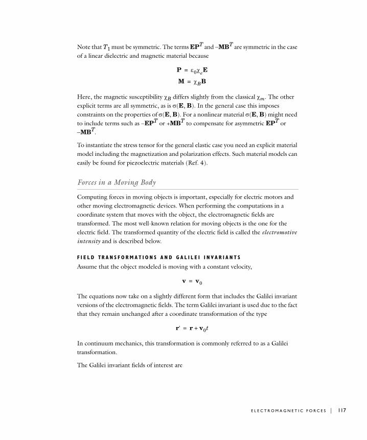
Note that T1 must be symmetric. The terms EPT and −MBT are symmetric in the case of a linear dielectric and magnetic material because
Here, the magnetic susceptibility χB differs slightly from the classical χm. The other explicit terms are all symmetric, as is σ(E, B). In the general case this imposes constraints on the properties of σ(E, B). For a nonlinear material σ(E, B) might need to include terms such as −EPT or +MBT to compensate for asymmetric EPT or −MBT.
To instantiate the stress tensor for the general elastic case you need an explicit material model including the magnetization and polarization effects. Such material models can easily be found for piezoelectric materials (Ref. 4).
Forces in a Moving Body
Computing forces in moving objects is important, especially for electric motors and other moving electromagnetic devices. When performing the computations in a coordinate system that moves with the object, the electromagnetic fields are transformed. The most well-known relation for moving objects is the one for the electric field. The transformed quantity of the electric field is called the electromotive intensity and is described below.
F I E L D TR A N S F O R M A T I O N S A N D G A L I L E I I N V A R I A N T S
Assume that the object modeled is moving with a constant velocity,
The equations now take on a slightly different form that includes the Galilei invariant versions of the electromagnetic fields. The term Galilei invariant is used due to the fact that they remain unchanged after a coordinate transformation of the type
In continuum mechanics, this transformation is commonly referred to as a Galilei transformation.
The Galilei invariant fields of interest are
P ε0χeE=
M χBB=
v v0=
r' r v0t+=
E L E C T R O M A G N E T I C F O R C E S | 117
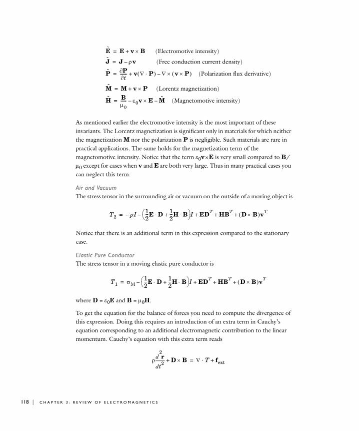
118 | C H A P T E R
As mentioned earlier the electromotive intensity is the most important of these invariants. The Lorentz magnetization is significant only in materials for which neither the magnetization M nor the polarization P is negligible. Such materials are rare in practical applications. The same holds for the magnetization term of the magnetomotive intensity. Notice that the term ε0v × E is very small compared to B/µ0 except for cases when v and E are both very large. Thus in many practical cases you can neglect this term.
Air and VacuumThe stress tensor in the surrounding air or vacuum on the outside of a moving object is
Notice that there is an additional term in this expression compared to the stationary case.
Elastic Pure ConductorThe stress tensor in a moving elastic pure conductor is
where D = ε0E and B = µ0H.
To get the equation for the balance of forces you need to compute the divergence of this expression. Doing this requires an introduction of an extra term in Cauchy’s equation corresponding to an additional electromagnetic contribution to the linear momentum. Cauchy’s equation with this extra term reads
E E v B (Electromotive intensity)×+=
J J ρv (Free conduction current density)–=
P P∂t∂
------- v ∇ P⋅( ) ∇ v P×( ) (Polarization flux derivative)×–+=
M M v P× (Lorentz magnetization)+=
H Bµ0------ ε0v E M–× (Magnetomotive intensity)–=
T2 pI–12---E D 1
2---H B⋅+⋅⎝ ⎠
⎛ ⎞ I– EDT HBT D B×( )vT+ + +=
T1 σM12---E D 1
2---H B⋅+⋅⎝ ⎠
⎛ ⎞ I– EDT HBT D B×( )vT+ + +=
ρt2
2
d
d r D B×+ ∇ T fext+⋅=
3 : R E V I E W O F E L E C T R O M A G N E T I C S
The extra term is canceled out by the additional term in the stress tensor, and the final result is
For the case of no acceleration, with the explicit appearance of the transformed quantities,
The terms containing v × B cancel out, which yields the following equation:
which is the same expression as for the stationary case.
General Elastic MaterialThe stress tensor for a moving general elastic material is
Notice that the magnetization M and the polarization P occur explicitly in this expression.
To instantiate the stress tensor for the general elastic case you need a material model explicitly including the magnetization and polarization effects as mentioned earlier in this section.
Electromagnetic Energy and Virtual Work
Another technique for computing forces is the one of deriving the electromagnetic energy of the system and computing the force by studying the effect of a small displacement. This is known as the method of virtual work or the principle of virtual displacement.
The method of virtual work is used for the electric energy and magnetic energy separately for computing the total electric or magnetic force as follows.
ρt2
2
d
d r ∇ σM⋅ ρE J B fext+×++=
0 ∇ σM⋅ ρ E v B×+( ) J ρv–( ) B fext+×++=
0 ∇ σM⋅ ρE J B fext+×++=
T1 σ E B,( )ε02-----E E 1
2µ0---------B B M B⋅–⋅+⋅⎝ ⎠
⎛ ⎞ I– ε0EET 1µ0------BBT
EPT MBT– ε0 E B×( )vT
+ +
+ +
=
E L E C T R O M A G N E T I C F O R C E S | 119
120 | C H A P T E R
M A G N E T I C F O R C E A N D TO R Q U E
The method of virtual work utilizes the fact that under constant magnetic flux conditions (Ref. 1), the total magnetic force on a system is computed as
If the system is constrained to rotate about an axis the torque is computed as
where is the rotational angle about the axis.
Under the condition of constant currents, the total force and torque are computed in the same way but with opposite signs,
E L E C T R I C F O R C E A N D TO R Q U E
Under the condition of constant charges, the total electric force and torque on a system are computed as
Under the condition of constant potentials, the total electric force and torque on a system are computed as
The functions cemforce and cemtorque in the AC/DC Module use the technique of virtual displacement. See the Function Reference in the AC/DC Module Reference Guide for details.
FΦ Wm∇–=
TΦ ϕ∂∂Wm–=
ϕ
FI Wm∇=
TI ϕ∂∂Wm=
FQ We∇–=
TQ ϕ∂∂We–=
FV We∇=
TV ϕ∂∂We=
3 : R E V I E W O F E L E C T R O M A G N E T I C S
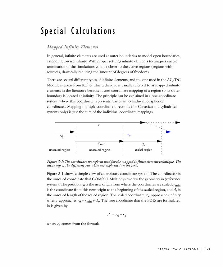
S p e c i a l C a l c u l a t i o n s
Mapped Infinite Elements
In general, infinite elements are used at outer boundaries to model open boundaries, extending toward infinity. With proper settings infinite elements techniques enable termination of the simulations volume closer to the active regions (regions with sources), drastically reducing the amount of degrees of freedoms.
There are several different types of infinite elements, and the one used in the AC/DC Module is taken from Ref. 6. This technique is usually referred to as mapped infinite elements in the literature because it uses coordinate mapping of a region so its outer boundary is located at infinity. The principle can be explained in a one-coordinate system, where this coordinate represents Cartesian, cylindrical, or spherical coordinates. Mapping multiple coordinate directions (for Cartesian and cylindrical systems only) is just the sum of the individual coordinate mappings.
Figure 3-1: The coordinate transform used for the mapped infinite element technique. The meaning of the different variables are explained in the text.
Figure 3-1 shows a simple view of an arbitrary coordinate system. The coordinate r is the unscaled coordinate that COMSOL Multiphysics draw the geometry in (reference system). The position r0 is the new origin from where the coordinates are scaled, rmin is the coordinate from this new origin to the beginning of the scaled region, and dr is the unscaled length of the scaled region. The scaled coordinate, rs, approaches infinity when r approaches r0 + rmin + dr. The true coordinate that the PDEs are formulated in is given by
where rs comes from the formula
r0
r
rmin
rs
unscaled regionunscaled region scaled region
dr
r' r0 rs+=
S P E C I A L C A L C U L A T I O N S | 121
122 | C H A P T E R
Lumped Parameter Conversion
When the impedance matrix, Z, or the admittance matrix, Y, is available it is possible to calculate all other types of lumped parameter matrices from the relations below.
where L is the inductance, C is the capacitance, R is the resistance, and G is the conductance. S is the S-parameter. The relations also include the following matrices
where Z0 is the characteristic impedance.
rs rmindr
rmin dr rminsgn r–+--------------------------------------------------------=
S Gref E Zref∗ Y⋅( ) E Zref Y⋅+( ) 1– Gref1–⋅ ⋅–⋅=
Z Y 1–=
L Im Z( ) ω⁄=
C Im Y( ) ω⁄=
R Re Z( )=
G Re Y( )=
E
1 0 0 00 1 0 00 0 1 00 0 0 1
=
Zref E Z0⋅=
Gref E 12 Re Z0( )------------------------------⋅=
3 : R E V I E W O F E L E C T R O M A G N E T I C S
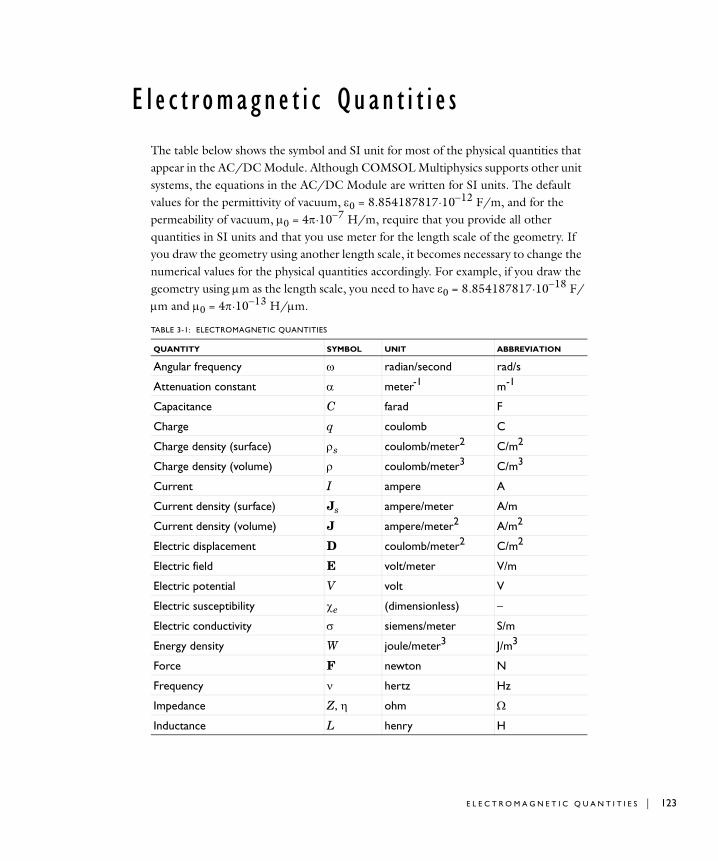
E l e c t r omagne t i c Quan t i t i e s
The table below shows the symbol and SI unit for most of the physical quantities that appear in the AC/DC Module. Although COMSOL Multiphysics supports other unit systems, the equations in the AC/DC Module are written for SI units. The default values for the permittivity of vacuum, ε0 = 8.854187817·10−12 F/m, and for the permeability of vacuum, µ0 = 4π·10−7 H/m, require that you provide all other quantities in SI units and that you use meter for the length scale of the geometry. If you draw the geometry using another length scale, it becomes necessary to change the numerical values for the physical quantities accordingly. For example, if you draw the geometry using µm as the length scale, you need to have ε0 = 8.854187817·10−18 F/µm and µ0 = 4π·10−13 H/µm.
TABLE 3-1: ELECTROMAGNETIC QUANTITIES
QUANTITY SYMBOL UNIT ABBREVIATION
Angular frequency ω radian/second rad/s
Attenuation constant α meter-1 m-1
Capacitance C farad F
Charge q coulomb C
Charge density (surface) ρs coulomb/meter2 C/m2
Charge density (volume) ρ coulomb/meter3 C/m3
Current I ampere A
Current density (surface) Js ampere/meter A/m
Current density (volume) J ampere/meter2 A/m2
Electric displacement D coulomb/meter2 C/m2
Electric field E volt/meter V/m
Electric potential V volt V
Electric susceptibility χe (dimensionless) −
Electric conductivity σ siemens/meter S/m
Energy density W joule/meter3 J/m3
Force F newton N
Frequency ν hertz Hz
Impedance Z, η ohm Ω
Inductance L henry H
E L E C T R O M A G N E T I C Q U A N T I T I E S | 123
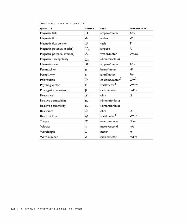
124 | C H A P T E R
Magnetic field H ampere/meter A/m
Magnetic flux Φ weber Wb
Magnetic flux density B tesla T
Magnetic potential (scalar) Vm ampere A
Magnetic potential (vector) A weber/meter Wb/m
Magnetic susceptibility χm (dimensionless) −
Magnetization M ampere/meter A/m
Permeability µ henry/meter H/m
Permittivity ε farad/meter F/m
Polarization P coulomb/meter2 C/m2
Poynting vector S watt/meter2 W/m2
Propagation constant β radian/meter rad/m
Reactance X ohm Ω
Relative permeability µr (dimensionless) −
Relative permittivity εr (dimensionless) −
Resistance R ohm Ω
Resistive loss Q watt/meter3 W/m3
Torque T newton-meter N·mVelocity v meter/second m/s
Wavelength λ meter m
Wave number k radian/meter rad/m
TABLE 3-1: ELECTROMAGNETIC QUANTITIES
QUANTITY SYMBOL UNIT ABBREVIATION
3 : R E V I E W O F E L E C T R O M A G N E T I C S
Re f e r e n c e s
1. D.K. Cheng, Field and Wave Electromagnetics, Addison-Wesley, 1991, 2nd edition.
2. Jianming Jin, The Finite Element Method in Electromagnetics, 2nd Edition, Wiley-IEEE Press, May 2002.
3. A. Kovetz, The Principles of Electromagnetic Theory, Cambridge University Press, 1990.
4. O. Wilson, Introduction to Theory and Design of Sonar Transducers, Peninsula Publishing, 1988.
5. R.K. Wangsness, Electromagnetic Fields, John Wiley & Sons, 1986, 2nd edition.
6. O.C. Zienkiewicz, C. Emson, and P. Bettess, “A Novel Boundary Infinite Element,” International Journal for Numerical Methods in Engineering, vol. 19(3), pp. 393–404, 1983.
R E F E R E N C E S | 125

126 | C H A P T E R
3 : R E V I E W O F E L E C T R O M A G N E T I C S
4
T h e A p p l i c a t i o n M o d e s
The purpose of this chapter is to give the user a detailed summary of what the application modes contains. For example, what each boundary condition does and what the application mode properties means.
127
128 | C H A P T E R
Th e App l i c a t i o n Mode Fo rmu l a t i o n s
The application modes in the AC/DC Module form a complete set of simulation tools for electromagnetic field simulations. To select the right application mode for describing the real-life physics you need to consider the geometric properties and the time variations of the fields.
The application modes in the AC/DC Module are listed below with the physical quantity solved for and the standard abbreviation that is used for the application modes in COMSOL Multiphysics. The physical quantities used are
• the magnetic field H
• the electric scalar potential V
• the magnetic vector potential A
• the magnetic scalar potential Vm
You can also use the application modes with the COMSOL Script or MATLAB. See “Programming Reference” on page 59 in the AC/DC Module Reference Guide for details.
Application Mode Guide
Table 4-1 on page 129 lists the available application modes in the AC/DC Module. For a descriptive illustration and more details on each of these modes, see the corresponding section in the table’s Page column.
In the Name column you find the default name that is given to the application mode. This name appears as a label on the application mode when you use it and is of special importance when performing multiphysics simulations in order to distinguish between different application modes in the model. The variables defined by the application modes get an underscore plus the application mode name appended to their names.
The Dependent Variables column contains the variables that the PDEs are formulated for. For most 2D modes, the PDEs solved in the simulations are formulated for the components that are perpendicular to the modeling plane. For axisymmetric simulations, COMSOL Multiphysics makes a variable transformation to avoid singularities at the rotation axis.
4 : T H E A P P L I C A T I O N M O D E S
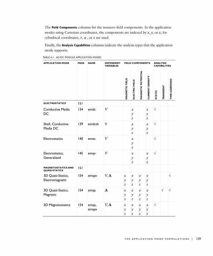
The Field Components columns list the nonzero field components. In the application modes using Cartesian coordinates, the components are indexed by x, y, or z; for cylindrical coordinates, r, , or z are used.
Finally, the Analysis Capabilities columns indicate the analysis types that the application mode supports.
TABLE 4-1: AC/DC MODULE APPLICATION MODES
APPLICATION MODE PAGE NAME DEPENDENT VARIABLES
FIELD COMPONENTS ANALYSIS CAPABILITIES
MA
GN
ET
IC F
IEL
D
EL
EC
TR
IC F
IEL
D
MA
GN
ET
IC P
OT
EN
TIA
L
CU
RR
EN
T D
EN
SIT
Y
ST
AT
IC
TR
AN
SIE
NT
TIM
E-H
AR
MO
NIC
ELECTROSTATICS 151
Conductive Media DC
134 emdc V x y z
x y z
√
Shell, Conductive Media DC
139 emdcsh V x y z
x y z
√
Electrostatics 140 emes V x y z
√
Electrostatics, Generalized
145 emqv V x y z
x y z
√
MAGNETOSTATICS AND QUASI-STATICS
151
3D Quasi-Statics, Electromagnetic
154 emqav V, A x y z
x y z
x y z
x y z
√
3D Quasi-Statics, Magnetic
154 emqa A x y z
x y z
x y z
x y z
√ √
3D Magnetostatics 154 emqa, emqav
V, A x y z
x y z
x y z
x y z
√
ϕ
T H E A P P L I C A T I O N M O D E F O R M U L A T I O N S | 129
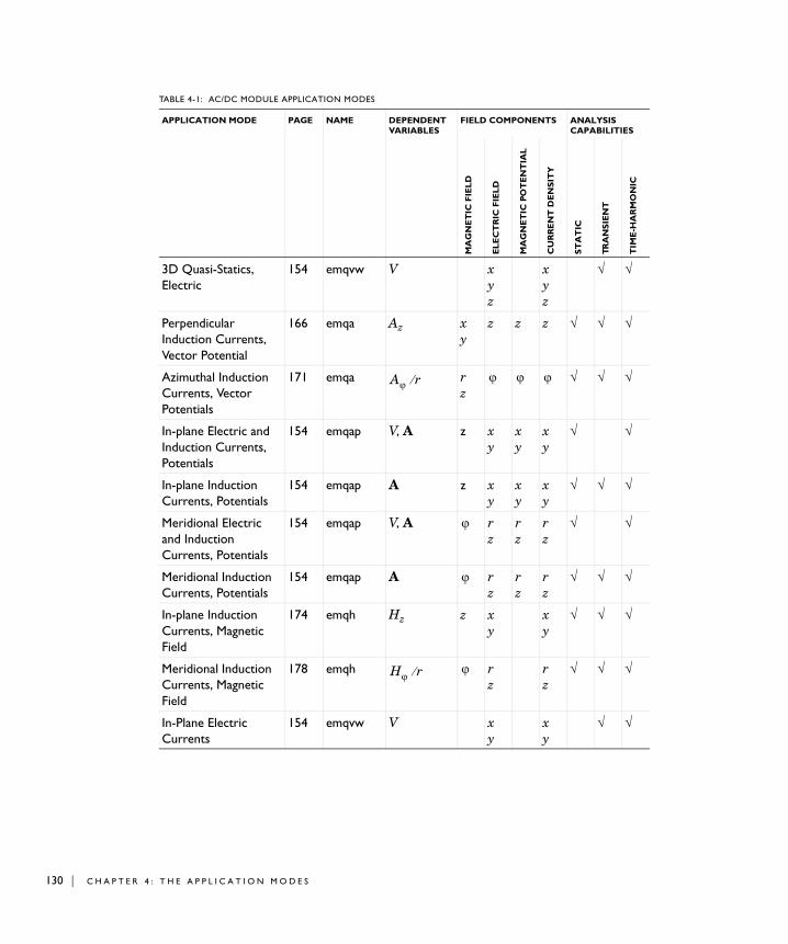
130 | C H A P T E R
3D Quasi-Statics, Electric
154 emqvw V x y z
x y z
√ √
Perpendicular Induction Currents, Vector Potential
166 emqa Az x y
z z z √ √ √
Azimuthal Induction Currents, Vector Potentials
171 emqa r z
√ √ √
In-plane Electric and Induction Currents, Potentials
154 emqap V, A z x y
x y
x y
√ √
In-plane Induction Currents, Potentials
154 emqap A z x y
x y
x y
√ √ √
Meridional Electric and Induction Currents, Potentials
154 emqap V, A r z
r z
r z
√ √
Meridional Induction Currents, Potentials
154 emqap A r z
r z
r z
√ √ √
In-plane Induction Currents, Magnetic Field
174 emqh Hz z x y
x y
√ √ √
Meridional Induction Currents, Magnetic Field
178 emqh r z
r z
√ √ √
In-Plane Electric Currents
154 emqvw V x y
x y
√ √
TABLE 4-1: AC/DC MODULE APPLICATION MODES
APPLICATION MODE PAGE NAME DEPENDENT VARIABLES
FIELD COMPONENTS ANALYSIS CAPABILITIES
MA
GN
ET
IC F
IEL
D
EL
EC
TR
IC F
IEL
D
MA
GN
ET
IC P
OT
EN
TIA
L
CU
RR
EN
T D
EN
SIT
Y
ST
AT
IC
TR
AN
SIE
NT
TIM
E-H
AR
MO
NIC
Aϕ r⁄ ϕ ϕ ϕ
ϕ
ϕ
Hϕ r⁄ ϕ
4 : T H E A P P L I C A T I O N M O D E S
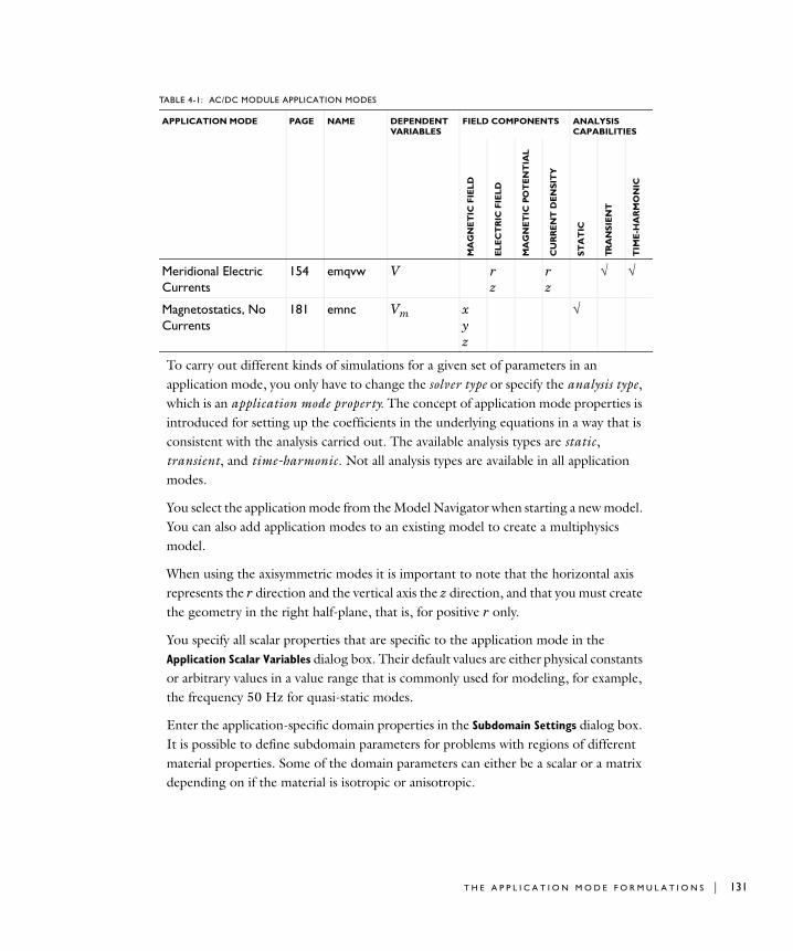
To carry out different kinds of simulations for a given set of parameters in an application mode, you only have to change the solver type or specify the analysis type, which is an application mode property. The concept of application mode properties is introduced for setting up the coefficients in the underlying equations in a way that is consistent with the analysis carried out. The available analysis types are static, transient, and time-harmonic. Not all analysis types are available in all application modes.
You select the application mode from the Model Navigator when starting a new model. You can also add application modes to an existing model to create a multiphysics model.
When using the axisymmetric modes it is important to note that the horizontal axis represents the r direction and the vertical axis the z direction, and that you must create the geometry in the right half-plane, that is, for positive r only.
You specify all scalar properties that are specific to the application mode in the Application Scalar Variables dialog box. Their default values are either physical constants or arbitrary values in a value range that is commonly used for modeling, for example, the frequency 50 Hz for quasi-static modes.
Enter the application-specific domain properties in the Subdomain Settings dialog box. It is possible to define subdomain parameters for problems with regions of different material properties. Some of the domain parameters can either be a scalar or a matrix depending on if the material is isotropic or anisotropic.
Meridional Electric Currents
154 emqvw V r z
r z
√ √
Magnetostatics, No Currents
181 emnc Vm x y z
√
TABLE 4-1: AC/DC MODULE APPLICATION MODES
APPLICATION MODE PAGE NAME DEPENDENT VARIABLES
FIELD COMPONENTS ANALYSIS CAPABILITIES
MA
GN
ET
IC F
IEL
D
EL
EC
TR
IC F
IEL
D
MA
GN
ET
IC P
OT
EN
TIA
L
CU
RR
EN
T D
EN
SIT
Y
ST
AT
IC
TR
AN
SIE
NT
TIM
E-H
AR
MO
NIC
T H E A P P L I C A T I O N M O D E F O R M U L A T I O N S | 131
132 | C H A P T E R
The Boundary Settings dialog box also adapts to the current application mode and lets you select application-specific boundary conditions. A certain boundary type might require one or several fields to be specified, while others generate the boundary conditions without user-specified fields.
The Edge Settings and Point Settings dialog boxes similarly let you specify application-specific conditions on edges and points.
Finally, use the Plot Parameters, Cross-Section Plot Parameters, and Domain Plot
Parameters dialog boxes to visualize the relevant physical variables for all application modes in the model. The nonzero components of the electromagnetic vector fields contain the name of the coordinate; for example, Aphi is the component of the magnetic vector potential.
The remainder of this chapter contains all the details necessary to get full insight into the different application modes, that is, the physical assumptions and mathematical considerations they are based on and all the functionality that is available. Each section describing a particular mode is divided into the following sections:
In the PDE Formulation section, the equation or equations that are solved in the application mode are derived.
In the Application Mode Properties section you find properties that are specific for the application mode. You can use these properties to, for example, select the analysis type.
The Application Scalar Variables section lists the parameters that are specific for the application mode. Their default values are either physical constants or arbitrary values in a value range that is commonly used for modeling, for example, the frequency 50 Hz for quasi-static modes.
The Boundary and Interface Conditions section contains the available boundary conditions and explanations of their physical interpretation.
In the Line Sources and Point Sources sections you find the available settings on edges and points, respectively.
Information about the Application Mode Variables can be found in Chapter 2, “The Application Modes,” in the AC/DC Module Reference Guide. That section lists all variables that are available in postprocessing and when formulating the equations. You can use any function of these variables when postprocessing the result of the analysis. It is also possible to use these variables in the expressions for the physical properties in the equations.
ϕ
4 : T H E A P P L I C A T I O N M O D E S
M A T E R I A L L I B R A R Y
All application modes in the AC/DC Module support the use of the COMSOL Multiphysics material libraries. The electromagnetic material properties that you can store in the material databases are:
• The electric conductivity and resistivity.
• The relative permittivity
• The relative permeability
• Nonlinear BH-curves.
• The refractive index
In addition, the AC/DC Module provides a special AC/DC Material Properties library, which contains electromagnetic and other material properties for materials such as soft iron, samarium-cobalt alloy, and graphite. Some properties depend on the magnetic flux density, location, or temperature. An additional tabbed page for, Electric
(AC/DC), appears in the Materials/Coefficients Library dialog box. It can contain, depending on the material, the following additional properties:
• Remanent flux density
• Reference temperature
• Temperature coefficient
• Nonlinear BH-curves
• Resistivity at reference temperature
For an example of a model using these properties to model samarium cobalt magnets and soft iron with a nonlinear B-H curve, see “Generator in 2D” on page 39 in the AC/DC Module Model Library.
See “Using the Materials/Coefficients Library” on page 223 in the COMSOL Multiphysics User’s Guide for details about the material and coefficients libraries.
T H E A P P L I C A T I O N M O D E F O R M U L A T I O N S | 133
134 | C H A P T E R
E l e c t r o s t a t i c F i e l d s
Modeling of static electric fields is carried out using the electric potential V. By combining the definition of the potential with Gauss’ law and the equation of continuity, you can derive the classical Poisson’s equation.
Under static conditions, the electric potential V is defined by the equivalence
Using this together with the constitutive relation D = ε0E + P between D and E, you can rewrite Gauss’ law as Poisson’s equation
This equation holds for nonconducting media and is used in the Electrostatics application mode. When handling conducting media, the equation of continuity is considered. In a stationary coordinate system, the point form of Ohm’s law states that
where Je is an externally generated current density. The static form of the equation of continuity then gives us
To handle current sources the equation can be generalized to
This equation forms the basis for the Conductive Media DC application mode.
Conductive Media DC Application Mode
The Conductive Media DC application mode is available for 3D, 2D in-plane, and 2D axisymmetric models.
P D E F O R M U L A T I O N
In the Conductive Media DC application mode the equation
E V∇–=
∇– ε0 V∇ P–( )⋅ ρ=
J σE Je+=
∇ J⋅ ∇– σ V∇ Je–( )⋅ 0= =
∇– σ V∇ Je–( )⋅ Qj=
∇– σ V∇ Je–( )⋅ Qj=
4 : T H E A P P L I C A T I O N M O D E S
is solved.
The in-plane Conductive Media DC application mode assumes that your model has a symmetry where the electric potential varies only in the x and y directions and is constant in the z direction. This implies that the electric field E is tangential to the x-y plane. The application mode solves the following equation where d is the thickness in the z direction.
The axisymmetric Conductive Media DC application mode is useful in the situation where the fields and the geometry are axially symmetric. In this case the electric potential is constant in the direction, which implies that the electric field is tangential to the rz-plane.
Writing the equation in cylindrical coordinates and multiplying it by r to avoid singularities at r = 0, the equation becomes
Specifying the ConductivityYou can provide the conductivity using two different types of conductivity relations:
• The conductivity, either as an isotropic conductivity (a scalar number or expression) or as an anisotropic conductivity, using several components of a conductivity tensor to define an anisotropic material. See “Modeling Anisotropic Material” on page 215 in the COMSOL Multiphysics User’s Guide for information about entering anisotropic material properties.
• A linear temperature relation for modeling a temperature-dependent conductivity (Joule heating or resistive heating). In this case the following equation describes the conductivity:
where ρ0 is the resistivity at the reference temperature T0. α is the temperature coefficient of resistivity, which describes how the resistivity varies with temperature. T is the current temperature, which can be a value that you specify or the
∇– d σ V∇ Je–( )⋅ dQj=
ϕ
r∂∂
z∂∂
T
– rσ r∂∂V
z∂∂V
rJe–
⎝ ⎠⎜ ⎟⎜ ⎟⎜ ⎟⎜ ⎟⎛ ⎞
⋅ rQj=
σ 1ρ0 1 α T T0–( )+( )-----------------------------------------------=
E L E C T R O S T A T I C F I E L D S | 135
136 | C H A P T E R
temperature from a heat transfer application mode (in the Joule Heating predefined multiphysics coupling, this is the default setting).
Select the type of conductivity from the Conductivity relation list.
B O U N D A R Y C O N D I T I O N S
The relevant interface condition at interfaces between different media for this mode is
This is fulfilled by the natural boundary condition
Current FlowThe current flow boundary condition
specifies the normal component of the current density flowing across the boundary.
Inward Current FlowThe inward current flow boundary condition
is similar to the above current flow boundary condition. In this case you specify the normal component of the current density rather than the complete vector. When the normal component Jn is positive the current flows inward through the boundary.
Distributed ResistanceYou can use the distributed resistance boundary condition
to model a thin sheet of a resistive material. The sheet has thickness d and is connected to the potential Vref.
Electric InsulationThe electric insulation boundary condition
n2 J1 J2–( )⋅ 0=
n σ V∇ Je–( )1 σ V∇ Je
–( )2–[ ]⋅ n– J1 J2–( )⋅ 0= =
n J⋅ n J0⋅=
n J⋅– Jn=
n J⋅ σd--- V Vref–( ),= n J1 J2–( )⋅ σ
d--- V Vref–( )=
n J⋅ 0=
4 : T H E A P P L I C A T I O N M O D E S
specifies that there is no current flowing across the boundary.
You can also use this boundary condition at symmetry boundaries where the potential is known to be symmetric with respect to the boundary.
Electric PotentialThe electric potential boundary condition
specifies the voltage at the boundary. Because the potential is the dependent variable that the application mode solves for, its value has to be defined at some point or boundary in the geometry to be fully determined.
GroundThe ground boundary condition
is a special case of the previous one specifying a zero potential. You can also use this boundary condition at symmetry boundaries, where the potential is known to be antisymmetric with respect to the boundary.
Current SourceThe current source boundary condition
represents either a source or a sink of current at interior boundaries.
ContinuityThe continuity boundary condition
specifies that the normal component of the electric current is continuous across the interior boundary.
Floating PotentialTo set a floating potential with an integral constraint, use this boundary condition:
V V0=
V 0=
n J1 J2–( )⋅ Jn=
n J1 J2–( )⋅ 0=
n J1 J2–( )⋅Ω∂∫ I0= n J⋅–
Ω∂∫ I0=
E L E C T R O S T A T I C F I E L D S | 137
138 | C H A P T E R
This sets the potential to a constant value on the boundary such that the integral is fulfilled. See the section “Floating Potentials and Electric Shielding” on page 17 for an example.
Circuit TerminalThe circuit terminal is a special version of the floating potential boundary condition specialized for connection to external circuits. See the section “SPICE Circuit Import” on page 70 for more information.
Electric ShieldingThe electric shielding boundary condition describes a thin layer of a dielectric medium that shields the electric field. See the section “Floating Potentials and Electric Shielding” on page 17 for an example.
PortUse the port condition on the electrodes to calculate the conductance or resistance. This condition forces the potential or current to one or zero depending on the settings. See the section “The Port Page” on page 50 for more information about port conditions.
Contact ResistanceYou can use the contact resistance boundary condition
to model a thin layer of a resistive material. The layer has the thickness d and the conductivity σ. This boundary condition is only available at the border between the parts in an assembly.
Axial SymmetryUse the axial symmetry boundary condition on the symmetry axis r = 0 in axisymmetric models only. For a thorough discussion of this boundary condition, see “Axial Symmetry” on page 149 for the generalized electrostatic formulation.
Periodic Boundary ConditionThe periodic boundary condition sets up a periodicity between the selected boundaries. See section “Periodic Boundary Conditions” on page 26 for more details on this boundary condition.
n J⋅( )1σd--- V1 V2–( )=
n J⋅( )2σd--- V2 V1–( )=
4 : T H E A P P L I C A T I O N M O D E S
L I N E S O U R C E S
In 3D line sources can be specified along the edges of the geometry.
Line Current SourceA line current source Qjl can be applied to edges. This source represents electric current per unit length.
PO I N T S O U R C E S A N D C O N S T R A I N T S
Point sources and constraints can be specified in 2D and 3D.
Point Current SourceA point current source Qj0 can be applied to points. This source represents an electric current flowing out of the point.
Point Constraint (Electric Potential)The electric potential can be constrained to the value V0 in a point using a constraint.
A P P L I C A T I O N M O D E VA R I A B L E S
See the section “Conductive Media DC Application Mode” on page 5 of the AC/DC Module Reference Guide.
Shell, Conductive Media DC Application Mode
You can use the Shell, Conductive Media DC application mode in 3D to model thin shells of conductive media. This application mode is similar to the 2D Conductive Media DC application mode. It solves the problem on 2D surfaces in a 3D geometry. The difference is that the shell does not have to be flat as they obviously are when using the 2D Conductive Media DC application mode.
P D E F O R M U L A T I O N
The application mode solves the following equation where d is the thickness of the shell:
The operator represents the tangential derivative along the shell.
For boundary conditions and application mode variables see the section “Conductive Media DC Application Mode” on page 134.
∇t d σ∇tV Je–( )⋅– dQj=
∇t
E L E C T R O S T A T I C F I E L D S | 139
140 | C H A P T E R
Electrostatics Application Mode
You can use the Electrostatics application mode for 3D, 2D in-plane and 2D axisymmetric models.
Applications involving electrostatics include high-voltage apparatus, electronic devices, and capacitors. The statics means that the time rate of change is slow and that wavelengths are very large compared to the size of the domain of interest.
P D E F O R M U L A T I O N
The 3D Electrostatics application mode solves the equation
This equation assumes the constitutive relation D = ε0E + P. The corresponding equations for the constitutive relations D = ε0εrE and D = ε0εrE + Dr can also be handled.
The in-plane Electrostatics application mode assumes a symmetry where the electric potential varies only in the x and y directions and is constant in the z direction. This implies that the electric field E is tangential to the xy-plane. Given this symmetry, it solves the same equation as in the 3D case.
Use the axisymmetric Electrostatics application mode when the fields and the geometry are axially symmetric. In this case, the electric potential is constant in the
direction, which implies that the electric field is tangential to the rz-plane.
Writing the equation in cylindrical coordinates and multiplying it by r to avoid singularities at r = 0, the equation becomes
A P P L I C A T I O N S C A L A R V A R I A B L E S
The application-specific scalar variable in this mode is given below.
PROPERTY NAME DEFAULT DESCRIPTION
ε0 epsilon0 8.854187817·10-12 F/m Permittivity of vacuum
∇– ε0 V∇ P–( )⋅ ρ=
ϕ
r∂∂
z∂∂
T
– rε0r∂
∂V
z∂∂V
rP–
⎝ ⎠⎜ ⎟⎜ ⎟⎜ ⎟⎜ ⎟⎛ ⎞
⋅ rρ=
4 : T H E A P P L I C A T I O N M O D E S
B O U N D A R Y C O N D I T I O N S
The relevant interface condition at interfaces between different media for this application mode is
In the absence of surface charges this is fulfilled by the natural boundary condition
Electric DisplacementUse the electric displacement boundary condition
to specify the normal component of the electric displacement at a boundary.
Surface ChargeThe surface charge boundary condition
makes it possible to specify the surface charge density at an exterior boundary or at the interior boundary between two media.
Zero Charge/SymmetryThe zero charge/symmetry boundary condition
specifies that the normal component of the electric displacement is zero.
You can also use this boundary condition at symmetry boundaries where the potential is known to be symmetric with respect to the boundary.
Electric PotentialThe electric potential boundary condition
specifies the voltage at the boundary. Because you are solving for the potential, it is necessary to define its value at some boundary in the geometry for the potential to be fully determined.
n2 D1 D2–( )⋅ ρs=
n ε0 V∇ P–( )1 ε0 V∇ P–( )2–[ ]⋅ n– D1 D2–( )⋅ 0= =
n D⋅ n D0⋅=
n– D⋅ ρs,= n D1 D2–( )⋅ ρs=
n D⋅ 0=
V V0=
E L E C T R O S T A T I C F I E L D S | 141
142 | C H A P T E R
GroundThe ground boundary condition
is a special case of the previous one specifying a zero potential. You can also use this boundary condition at symmetry boundaries, where the potential is known to be antisymmetric with respect to the boundary.
PortUse the port condition on the electrodes to calculate the capacitance. This condition forces the potential to one or zero depending on the settings (see the section “Lumped Parameters” on page 47).
Electric ShieldingThe electric shielding boundary condition describes a thin layer of a dielectric medium that shields the electric field. See the section “Floating Potentials and Electric Shielding” on page 17 for an example.
Floating PotentialTo set a floating potential with an integral constraint, use the boundary condition
which sets the potential to a constant value on the boundary such that the total charge is equal to Q0. See the section “Floating Potentials and Electric Shielding” on page 17 for an example.
ContinuityThe continuity boundary condition
specifies that the normal component of the electric displacement is continuous across the interior boundary.
Thin Low Permittivity GapUse the thin low permittivity gap condition
V 0=
ρs
Ω∂∫ Q0=
n D1 D2–( )⋅ 0=
4 : T H E A P P L I C A T I O N M O D E S
to model a thin gap of a material with a small permittivity compared to the adjacent domains. The gap has the thickness d and the relative permittivity εr. This boundary condition is only available at the border between parts in an assembly.
Axial SymmetryApply the axial symmetry boundary condition to the symmetry axis r = 0 in axisymmetric models.
Periodic Boundary ConditionThe periodic boundary condition sets up a periodicity between the selected boundaries. See section “Periodic Boundary Conditions” on page 26 for more details on this boundary condition.
L I N E S O U R C E S
In 3D line sources can be specified along the edges of the geometry.
Line ChargeA line charge Ql can be applied along the edges. The source is interpreted as electric charge per unit length.
PO I N T S O U R C E S A N D C O N S T R A I N T S
Point charges and point constraints are available in 2D and 3D.
Point ChargeA point charge Q0 can be applied to points.
Point Constraint (Electric Potential)The electric potential can be constrained to the value V0 in a point.
A P P L I C A T I O N M O D E VA R I A B L E S
See the section “The Electrostatics Application Mode” on page 7 in the AC/DC Module Reference Guide.
n D⋅( )1εd--- V1 V2–( )=
n D⋅( )2εd--- V2 V1–( )=
E L E C T R O S T A T I C F I E L D S | 143
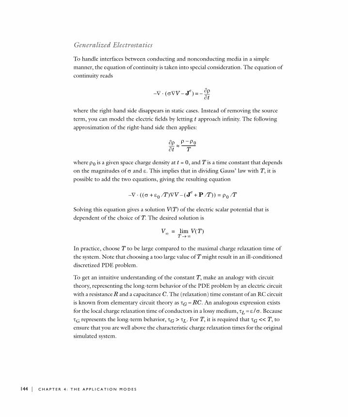
144 | C H A P T E R
Generalized Electrostatics
To handle interfaces between conducting and nonconducting media in a simple manner, the equation of continuity is taken into special consideration. The equation of continuity reads
where the right-hand side disappears in static cases. Instead of removing the source term, you can model the electric fields by letting t approach infinity. The following approximation of the right-hand side then applies:
where ρ0 is a given space charge density at t = 0, and T is a time constant that depends on the magnitudes of σ and ε. This implies that in dividing Gauss’ law with T, it is possible to add the two equations, giving the resulting equation
Solving this equation gives a solution V(T) of the electric scalar potential that is dependent of the choice of T. The desired solution is
In practice, choose T to be large compared to the maximal charge relaxation time of the system. Note that choosing a too large value of T might result in an ill-conditioned discretized PDE problem.
To get an intuitive understanding of the constant T, make an analogy with circuit theory, representing the long-term behavior of the PDE problem by an electric circuit with a resistance R and a capacitance C. The (relaxation) time constant of an RC circuit is known from elementary circuit theory as τG = RC. An analogous expression exists for the local charge relaxation time of conductors in a lossy medium, τL = ε/σ. Because τG represents the long-term behavior, τG > τL. For T, it is required that τG << T, to ensure that you are well above the characteristic charge relaxation times for the original simulated system.
∇– σ V∇ Je–( )⋅
t∂∂ρ–=
t∂∂ρ ρ ρ0–
T---------------≈
∇ σ ε0 T⁄+( ) V∇ Je P T⁄+( )–( )⋅ ρ0 T⁄=–
V∞ V T( )T ∞→lim=
4 : T H E A P P L I C A T I O N M O D E S
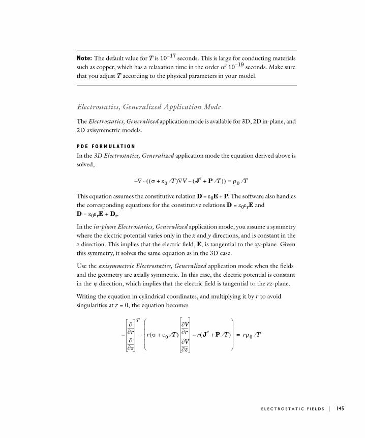
Note: The default value for T is 10−17 seconds. This is large for conducting materials such as copper, which has a relaxation time in the order of 10−19 seconds. Make sure that you adjust T according to the physical parameters in your model.
Electrostatics, Generalized Application Mode
The Electrostatics, Generalized application mode is available for 3D, 2D in-plane, and 2D axisymmetric models.
P D E F O R M U L A T I O N
In the 3D Electrostatics, Generalized application mode the equation derived above is solved,
This equation assumes the constitutive relation D = ε0E + P. The software also handles the corresponding equations for the constitutive relations D = ε0εrE and D = ε0εrE + Dr.
In the in-plane Electrostatics, Generalized application mode, you assume a symmetry where the electric potential varies only in the x and y directions, and is constant in the z direction. This implies that the electric field, E, is tangential to the xy-plane. Given this symmetry, it solves the same equation as in the 3D case.
Use the axisymmetric Electrostatics, Generalized application mode when the fields and the geometry are axially symmetric. In this case, the electric potential is constant in the direction, which implies that the electric field is tangential to the rz-plane.
Writing the equation in cylindrical coordinates, and multiplying it by r to avoid singularities at r = 0, the equation becomes
∇ σ ε0 T⁄+( ) V∇ Je P T⁄+( )–( )⋅ ρ0 T⁄=–
ϕ
r∂∂
z∂∂
T
– r σ ε0 T⁄+( ) r∂∂V
z∂∂V
r Je P T⁄+( )–
⎝ ⎠⎜ ⎟⎜ ⎟⎜ ⎟⎜ ⎟⎛ ⎞
⋅ rρ0 T⁄=
E L E C T R O S T A T I C F I E L D S | 145
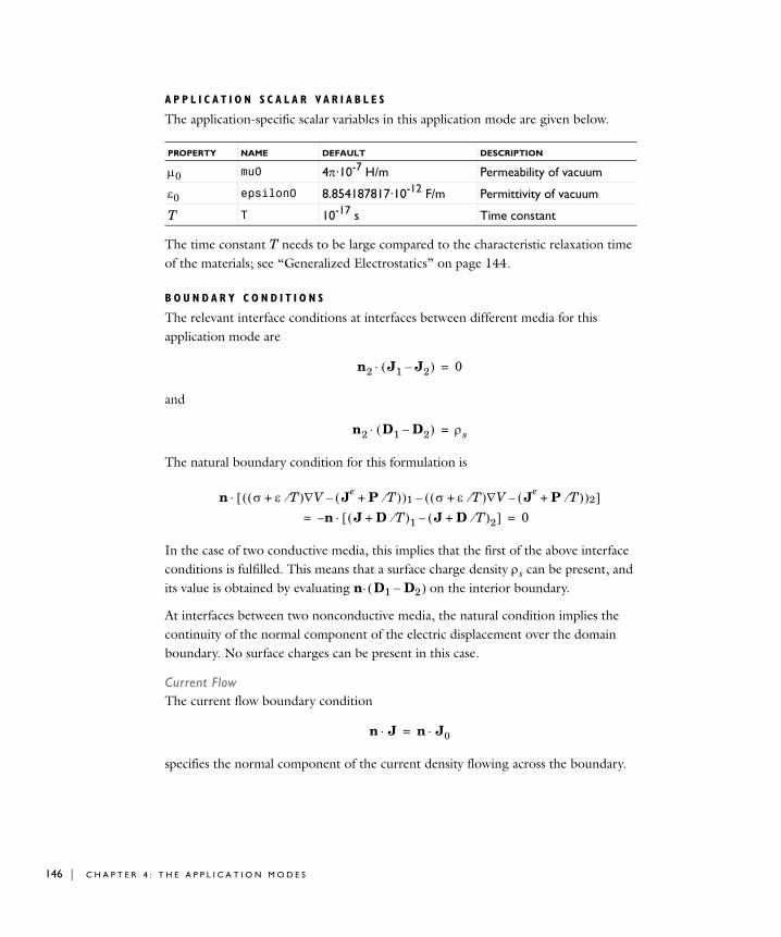
146 | C H A P T E R
A P P L I C A T I O N S C A L A R V A R I A B L E S
The application-specific scalar variables in this application mode are given below.
The time constant T needs to be large compared to the characteristic relaxation time of the materials; see “Generalized Electrostatics” on page 144.
B O U N D A R Y C O N D I T I O N S
The relevant interface conditions at interfaces between different media for this application mode are
and
The natural boundary condition for this formulation is
In the case of two conductive media, this implies that the first of the above interface conditions is fulfilled. This means that a surface charge density ρs can be present, and its value is obtained by evaluating n· ( D1 − D2 ) on the interior boundary.
At interfaces between two nonconductive media, the natural condition implies the continuity of the normal component of the electric displacement over the domain boundary. No surface charges can be present in this case.
Current FlowThe current flow boundary condition
specifies the normal component of the current density flowing across the boundary.
PROPERTY NAME DEFAULT DESCRIPTION
µ0 mu0 4π·10-7 H/m Permeability of vacuum
ε0 epsilon0 8.854187817·10-12 F/m Permittivity of vacuum
T T 10-17 s Time constant
n2 J1 J2–( )⋅ 0=
n2 D1 D2–( )⋅ ρs=
n σ ε T⁄+( ) V∇ Je P T⁄+( )–( )1 σ ε T⁄+( ) V∇ Je P T⁄+( )–( )2–[ ]⋅
n J D T⁄+( )1 J D T⁄+( )2–[ ]⋅– 0= =
n J⋅ n J0⋅=
4 : T H E A P P L I C A T I O N M O D E S
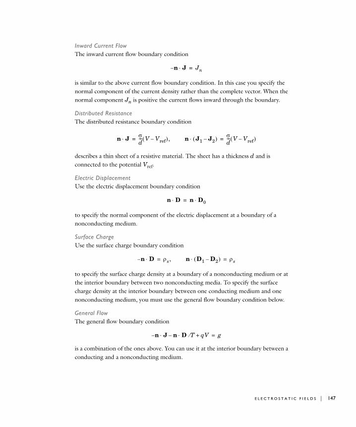
Inward Current FlowThe inward current flow boundary condition
is similar to the above current flow boundary condition. In this case you specify the normal component of the current density rather than the complete vector. When the normal component Jn is positive the current flows inward through the boundary.
Distributed ResistanceThe distributed resistance boundary condition
describes a thin sheet of a resistive material. The sheet has a thickness d and is connected to the potential Vref.
Electric DisplacementUse the electric displacement boundary condition
to specify the normal component of the electric displacement at a boundary of a nonconducting medium.
Surface ChargeUse the surface charge boundary condition
to specify the surface charge density at a boundary of a nonconducting medium or at the interior boundary between two nonconducting media. To specify the surface charge density at the interior boundary between one conducting medium and one nonconducting medium, you must use the general flow boundary condition below.
General FlowThe general flow boundary condition
is a combination of the ones above. You can use it at the interior boundary between a conducting and a nonconducting medium.
n J⋅– Jn=
n J⋅ σd--- V Vref–( ),= n J1 J2–( )⋅ σ
d--- V Vref–( )=
n D⋅ n D0⋅=
n– D⋅ ρs,= n D1 D2–( )⋅ ρs=
n– J n D⋅ T⁄– qV+⋅ g=
E L E C T R O S T A T I C F I E L D S | 147
148 | C H A P T E R
Electric InsulationThe electric insulation boundary condition
specifies that there is no current flowing across the boundary, and that the electric displacement is zero outside the boundary.
You can also use this boundary condition at symmetry boundaries where the potential is known to be symmetric with respect to the boundary.
Electric PotentialThe electric potential boundary condition
specifies the voltage at the boundary. Because you solve for the potential, it is necessary to define its value at some boundary or point in the geometry for the solution to be fully determined.
GroundThe ground boundary condition
is a special case of the previous one specifying a zero potential. You can also use this boundary condition at symmetry boundaries, where the potential is known to be antisymmetric with respect to the boundary.
Current SourceThe current source boundary condition
is applicable to interior boundaries that represent either a source or a sink of current. You can also use this boundary condition at an interior boundary between two conducting media.
General SourceThe general source boundary condition
n J D T⁄+( )⋅ 0=
V V0=
V 0=
n J1 J2–( )⋅ Jn=
n J1 J2–( ) n D1 D2–( )⋅ T⁄ q+ V+⋅ g=
4 : T H E A P P L I C A T I O N M O D E S
is a generalization of the surface charge and current source boundary condition. It can be used to define a source at an interior boundary between one conducting and one nonconducting medium.
ContinuityThe continuity boundary condition
specifies that the normal components of the electric current and electric displacement are continuous across the interior boundary.
Axial SymmetryUse the axial symmetry boundary condition on the symmetry axis r = 0 in axisymmetric models. This boundary condition is simply the natural Neumann boundary condition, which in the axisymmetric case is
The requirement that you must use this boundary condition on the z-axis comes from the symmetry reasons
The second equation can be rewritten as follows
This equation is fulfilled if the first of the conditions above is fulfilled all along the axis. This condition is in turn implied via the natural Neumann condition. Due to the numerical method, the boundary condition is evaluated for an r that is small but nonzero. This causes the radial component of the electric field to vanish along the axis.
L I N E S O U R C E S
In 3D, you can specify line sources along the edges of the geometry.
Line ChargeA line charge Ql can be applied along an edge around nonconducting media. The source is interpreted as electric charge per unit length.
n J1 J2–( ) D1 D2–( ) T⁄+( )⋅ 0=
n r σ ε T⁄+( ) V∇ r Je P T⁄+( )–( )⋅ 0=–
Er 0=
r∂∂Ez 0=
r∂∂Ez
r∂∂
z∂∂V
⎝ ⎠⎛ ⎞–
z∂∂
r∂∂V
⎝ ⎠⎛ ⎞–
z∂∂Er–= = =
E L E C T R O S T A T I C F I E L D S | 149
150 | C H A P T E R
Line Current SourceA line current source Qjl can be applied to edges around conducting media. This source represents electric current per unit length.
PO I N T S O U R C E S A N D C O N S T R A I N T S
Two types of point sources can be specified: electric charges and current sources. In addition you can specify the electric potential, which acts as a point constraint.
Point ChargeA point charge Q0 can be applied to points around nonconducting media.
Point Current SourceA point current source Qj0 can be applied to points around conducting media. This source represents an electric current flowing out of the point.
Point Constraint (Electric Potential)The electric potential can be constrained to the value V0 in a point.
A P P L I C A T I O N M O D E V A R I A B L E S
See the section “Electrostatics, Generalized Application Mode” on page 9 in the AC/DC Module Reference Guide.
4 : T H E A P P L I C A T I O N M O D E S
Magne t o s t a t i c a nd Qua s i - S t a t i c F i e l d s
Quasi-static analysis is valid under the assumption that ∂D / ∂t = 0. This implies that Maxwell’s equations can be rewritten in the following manner.
Here Je is an externally generated current density and v is the velocity of the conductor. The crucial criterion for the quasi-static approximation to be valid is that the currents and the electromagnetic fields vary slowly. This means that the dimensions of the structure in the problem need to be small compared to the wavelength.
Using the definitions of the potentials,
and the constitutive relation B = µ0(H + M), Ampère’s law can be rewritten as
The equation of continuity, which is obtained by taking the divergence of the above equation, gives us the equation
These two equations give us a system of equations for the two potentials A and V.
Magnetostatics
In the static case, the magnetostatics equations are
∇ H× J σ E v B×+( ) Je+= =
∇ E×t∂
∂B–=
∇ B⋅ 0=
∇ D⋅ ρ=
∇ J⋅ 0=
B ∇ A×=
E ∇V–t∂
∂A–=
σt∂
∂A ∇ µ01– ∇ A× M–( )× σv ∇ A×( ) σ V∇+×–+ Je
=
∇– σ A∂t∂
------- σv ∇ A×( ) σ∇V Je–+×–⎝ ⎠
⎛ ⎞⋅ 0=
M A G N E T O S T A T I C A N D Q U A S I - S T A T I C F I E L D S | 151
152 | C H A P T E R
The term represents the current generated motion with a constant velocity in a static magnetic field, JB = σ v × Be. Similarly the term represents a current generated by a static electric field, JE = σ Ee. When JB = 0, including JE in the external current results in the equation
with . You can solve this equation independently from the other equation.
Gauge Transformations
The electric and magnetic potentials are not uniquely defined from the electric and magnetic fields through
Introducing two new potentials
gives the same electric and magnetic fields:
The variable transformation of the potentials is called a gauge transformation. To obtain a unique solution you need to choose the gauge, that is, put constraints on Ψ that make the solution unique. Another way of expressing this additional condition is to put a constraint on . A vector field is uniquely defined up to a constant if both
and are given. This is called Helmholtz’s theorem. One particular gauge is the Coulomb gauge given by the constraint
∇– σv ∇ A×( ) σ∇V Je–+×–( )⋅ 0=
∇ µ01– ∇ A× M–( )× σv ∇ A×( ) σ V∇+×– Je
=
σv ∇ A×( )×σ V∇–
∇ µ01– ∇ A× M–( )× J
e=
Je
Je JE+=
E A∂t∂
-------– ∇V–=
B ∇ A×=
A A ∇Ψ+=
V V Ψ∂t∂
-------–=
E A∂t∂
-------– ∇V– A ∇Ψ–( )∂t∂
---------------------------– ∇ V Ψ∂t∂
-------+⎝ ⎠⎛ ⎞– A∂
t∂-------– ∇V–= = =
B ∇ A× ∇ A ∇Ψ–( )× ∇ A×= = =
∇ A⋅∇ A⋅ ∇ A×
4 : T H E A P P L I C A T I O N M O D E S
When using assemblies with interface pairs, it might also be necessary to activate an equation fixing a gauge. This has to be done when vector elements are coupled over a pair and the meshes on each side are incompatible. The gauge is the Coulomb gauge for Magnetostatics and Quasi-statics for electric and induction currents. Quasi-statics for induction currents uses other equations when fixing the gauge. These equations are shown below, where the first equation is for time-harmonic problems and the second equation is for transient problems.
Time-Harmonic Quasi-Statics
In the time-harmonic case, Ampère’s equation includes the displacement current:
In the transient case the inclusion of this term would lead to a second-order equation in time, but in the harmonic case there are no such complications. Using the definition of the electric and magnetic potentials, the system of equations becomes
The constitutive relation D = ε0E + P has been used for the electric field.
You obtain a particular gauge that reduces the system of equation by choosing Ψ = −jV / ωin the gauge transformation. This gives
Because vanishes from the equations, you only need the second one,
Working with à is often the best option when it is possible to specify all source currents as external currents Je or as surface currents on boundaries.
∇ A⋅ 0=
∇ J⋅ 0=
∇ σA( )⋅ 0=
∇ H× J σ E v B×+( ) jωD J+e
+= =
∇– jωσ ω2ε0–( )A σv ∇ A×( ) σ jωε0+( )∇V Je jωP+( )–+×–( )⋅ 0=
jωσ ω2ε0–( )A ∇ µ01– ∇ A M–×( )× σv ∇ A×( ) σ jωε0+( )∇V+×–+ Je jωP+=
A A jω----∇V–= V 0=
V
jωσ ω2ε0–( )A ∇ µ01– ∇ A M–×( )× σv ∇ A×( )×–+ Je jωP+=
M A G N E T O S T A T I C A N D Q U A S I - S T A T I C F I E L D S | 153
154 | C H A P T E R
Quasi-Statics for Electric Currents
If the skin depth in all domains is much larger than the geometry, you can make a further approximation by neglecting the coupling between the electric and magnetic fields. In other words, neglect the induced currents. In mathematical terms this approximation implies that
which means that you can express the electric field in terms of the electric potential only, . Combining the time-harmonic equation of continuity
with the equation
yields the following equation:
For the transient case, using the transient equation of continuity
the resulting equation becomes
3D and 2D Quasi-Statics Application Modes
With the quasi-statics application modes you can handle four classes of problems:
• Magnetostatics
• Time-harmonic quasi-statics with full coupling between the electric and magnetic fields
• Transient quasi-statics with partial coupling between the electric and magnetic field when the capacitive term can be neglected.
∇ E× 0=
E ∇V–=
∇ J⋅ ∇ σE Je+( )⋅ jωρ–= =
∇ D⋅ ρ=
∇– σ jωε0+( )∇V Je jωP+( )–( )⋅ 0=
∇ J⋅ ∇ σE Je+( )⋅
t∂∂ρ–= =
∇t∂
∂ ε0∇V P+( ) ∇ σ∇V Je–( )⋅–⋅– 0=
4 : T H E A P P L I C A T I O N M O D E S
• Time-harmonic quasi-statics in the case of electric currents when the coupling between the electric and magnetic fields can be neglected
• Transient quasi-statics for electric currents
In the 2D In-Plane Currents application modes the currents are only present in the plane. This implies that the magnetic field only has a component perpendicular to the plane. Similarly, in the Meridional Currents application mode the currents are only present in the rz-plane and the magnetic field only has a component.
P D E F O R M U L A T I O N S
MagnetostaticsFor magnetostatic problems there are two formulations available. In one of them, the system of equations
is solved. If v = 0 the equations decouple and can be solved independently. The other formulation is the single equation
The thickness d only appears in the 2D in-plane case and represents the thickness in the z direction.
Note: The conductivity cannot be zero anywhere when the electric potential is part of the problem, because the dependent variables then vanish from the first equation.
Induction Currents and Electric and Induction CurrentsAlso for quasi-static problem there are two formulations available. One formulation uses a system of equation for both the electric and magnetic potentials,
ϕ
∇– d σv ∇ A×( ) σ∇V Je–+×–( )⋅ 0=
∇ d µ01– ∇ A× M–( )× dσv ∇ A×( ) dσ V∇+×– dJe
=
∇ d µ01– ∇ A× M–( )× dJe
=
M A G N E T O S T A T I C A N D Q U A S I - S T A T I C F I E L D S | 155
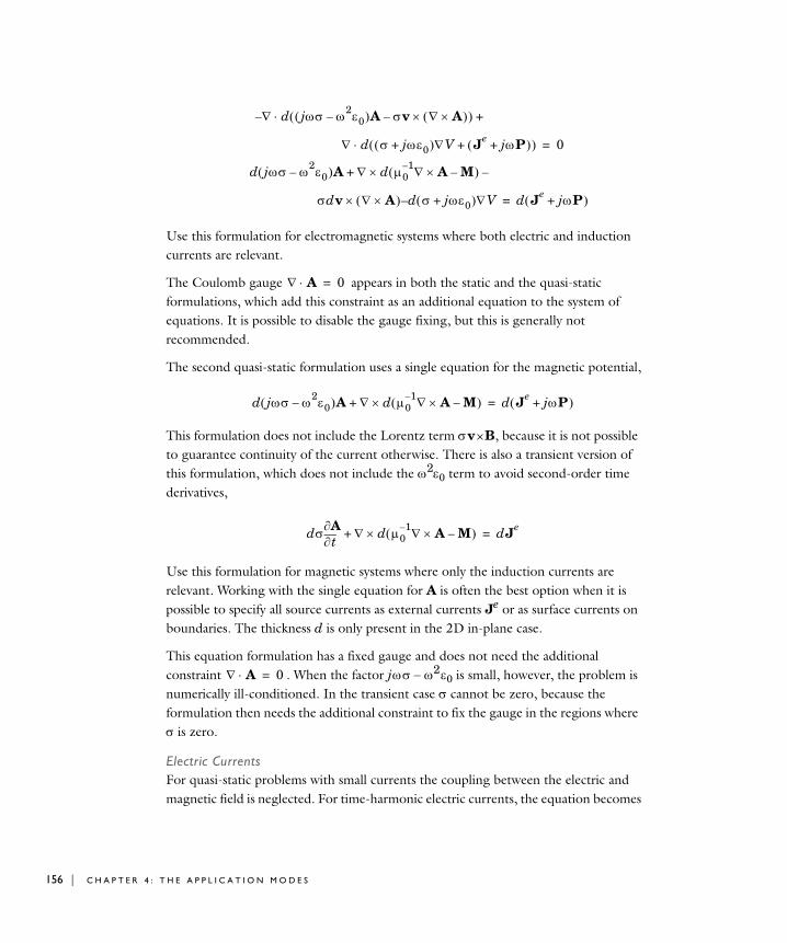
156 | C H A P T E R
Use this formulation for electromagnetic systems where both electric and induction currents are relevant.
The Coulomb gauge appears in both the static and the quasi-static formulations, which add this constraint as an additional equation to the system of equations. It is possible to disable the gauge fixing, but this is generally not recommended.
The second quasi-static formulation uses a single equation for the magnetic potential,
This formulation does not include the Lorentz term σ v × B, because it is not possible to guarantee continuity of the current otherwise. There is also a transient version of this formulation, which does not include the ω2ε0 term to avoid second-order time derivatives,
Use this formulation for magnetic systems where only the induction currents are relevant. Working with the single equation for A is often the best option when it is possible to specify all source currents as external currents Je or as surface currents on boundaries. The thickness d is only present in the 2D in-plane case.
This equation formulation has a fixed gauge and does not need the additional constraint . When the factor j ω σ − ω2 ε0 is small, however, the problem is numerically ill-conditioned. In the transient case σ cannot be zero, because the formulation then needs the additional constraint to fix the gauge in the regions where σ is zero.
Electric CurrentsFor quasi-static problems with small currents the coupling between the electric and magnetic field is neglected. For time-harmonic electric currents, the equation becomes
∇– d jωσ ω2ε0–( )A σv ∇ A×( )×–( ) +⋅
∇ d σ jωε0+( )∇V Je jωP+( )+( )⋅ 0=
d jωσ ω2ε0–( )A ∇ d µ01– ∇ A M–×( )× –+
σdv ∇ A×( ) d– σ jωε0+( )∇V× d Je jωP+( )=
∇ A⋅ 0=
d jωσ ω2ε0–( )A ∇ d µ01– ∇ A M–×( )×+ d Je jωP+( )=
dσt∂
∂A ∇ d µ01– ∇ A× M–( )×+ dJe
=
∇ A⋅ 0=
4 : T H E A P P L I C A T I O N M O D E S
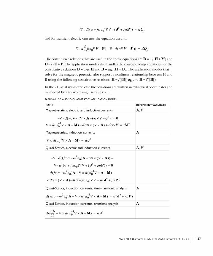
and for transient electric currents the equation used is:
.
The constitutive relations that are used in the above equations are B = µ0(H + M) and D = ε0E + P. The application modes also handles the corresponding equations for the constitutive relations B = µ0µrH and B = µ0µrH + Br. The application modes that solve for the magnetic potential also support a nonlinear relationship between H and B using the following constitutive relations: H = f ( | B | ) eB and H = f ( | B | ).
In the 2D axial symmetric case the equations are written in cylindrical coordinates and multiplied by r to avoid singularity at r = 0.
TABLE 4-2: 3D AND 2D QUASI-STATICS APPLICATION MODES
NAME DEPENDENT VARIABLES
Magnetostatics, electric and induction currents A, V
Magnetostatics, induction currents A
Quasi-Statics, electric and induction currents A, V
Quasi-Statics, induction currents, time-harmonic analysis A
Quasi-Statics, induction currents, transient analysis A
∇– d σ jωε0+( )∇V Je jωP+( )–( )⋅ dQj=
∇ dt∂
∂ ε0∇V P+( ) ∇ d σ∇V Je–( )⋅–( )⋅– dQj=
∇– d σv ∇ A×( ) σ∇V Je–+×–( )⋅ 0=
∇ d µ01– ∇ A× M–( )× dσv ∇ A×( ) dσ V∇+×– dJe
=
∇ d µ01– ∇ A× M–( )× dJe
=
∇– d jωσ ω2ε0–( )A σv ∇ A×( )×–( ) +⋅
∇ d σ jωε0+( )∇V Je jωP+( )+( )⋅ 0=
d jωσ ω2ε0–( )A ∇ d µ01– ∇ A M–×( )× –+
σdv ∇ A×( ) d– σ jωε0+( )∇V× d Je jωP+( )=
d jωσ ω2ε0–( )A ∇ d µ01– ∇ A M–×( )×+ d Je jωP+( )=
dσt∂
∂A ∇ d µ01– ∇ A× M–( )×+ dJe
=
M A G N E T O S T A T I C A N D Q U A S I - S T A T I C F I E L D S | 157
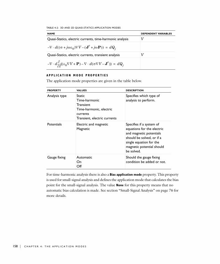
158 | C H A P T E R
A P P L I C A T I O N M O D E P R O P E R T I E S
The application mode properties are given in the table below.
For time-harmonic analysis there is also a Bias application mode property. This property is used for small-signal analysis and defines the application mode that calculates the bias point for the small-signal analysis. The value None for this property means that no automatic bias calculation is made. See section “Small-Signal Analysis” on page 76 for more details.
Quasi-Statics, electric currents, time-harmonic analysis V
Quasi-Statics, electric currents, transient analysis V
PROPERTY VALUES DESCRIPTION
Analysis type Static Time-harmonic Transient Time-harmonic, electric currents Transient, electric currents
Specifies which type of analysis to perform.
Potentials Electric and magnetic Magnetic
Specifies if a system of equations for the electric and magnetic potentials should be solved, or if a single equation for the magnetic potential should be solved.
Gauge fixing Automatic On Off
Should the gauge fixing condition be added or not.
TABLE 4-2: 3D AND 2D QUASI-STATICS APPLICATION MODES
NAME DEPENDENT VARIABLES
∇– d σ jωε0+( )∇V Je jωP+( )–( )⋅ dQj=
∇ dt∂
∂ ε0∇V P+( ) ∇ d σ∇V Je–( )⋅–( )⋅– dQj=
4 : T H E A P P L I C A T I O N M O D E S
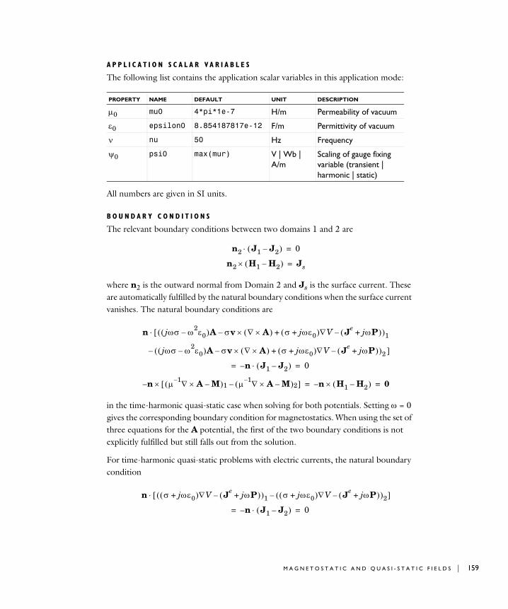
A P P L I C A T I O N S C A L A R V A R I A B L E S
The following list contains the application scalar variables in this application mode:
All numbers are given in SI units.
B O U N D A R Y C O N D I T I O N S
The relevant boundary conditions between two domains 1 and 2 are
where n2 is the outward normal from Domain 2 and Js is the surface current. These are automatically fulfilled by the natural boundary conditions when the surface current vanishes. The natural boundary conditions are
in the time-harmonic quasi-static case when solving for both potentials. Setting ω = 0 gives the corresponding boundary condition for magnetostatics. When using the set of three equations for the A potential, the first of the two boundary conditions is not explicitly fulfilled but still falls out from the solution.
For time-harmonic quasi-static problems with electric currents, the natural boundary condition
PROPERTY NAME DEFAULT UNIT DESCRIPTION
µ0 mu0 4*pi*1e-7 H/m Permeability of vacuum
ε0 epsilon0 8.854187817e-12 F/m Permittivity of vacuum
ν nu 50 Hz Frequency
ψ0 psi0 max(mur) V | Wb | A/m
Scaling of gauge fixing variable (transient | harmonic | static)
n2 J1 J2–( )⋅ 0=
n2 H1 H2–( )× Js=
n jωσ ω2ε0–( )A σv ∇ A×( ) σ jωε0+( )∇V Je jωP+( )–+×–( )1[⋅
jωσ ω2ε0–( )A σv ∇ A×( ) σ jωε0+( )∇V Je jωP+( )–+×–( )2 ]–
n– J1 J2–( )⋅ 0= =
n µ 1– ∇ A× M–( )1 µ 1– ∇ A× M–( )2–[ ]×– n H1 H2–( )×– 0= =
n σ jωε0+( )∇V Je jωP+( )–( )1 σ jωε0+( )∇V Je jωP+( )–( )2–[ ]⋅
n– J1 J2–( )⋅ 0= =
M A G N E T O S T A T I C A N D Q U A S I - S T A T I C F I E L D S | 159
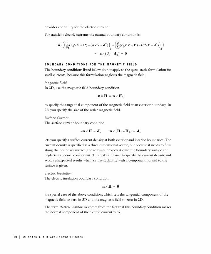
160 | C H A P T E R
provides continuity for the electric current.
For transient electric currents the natural boundary condition is:
B O U N D A R Y C O N D I T I O N S F O R T H E M A G N E T I C F I E L D
The boundary conditions listed below do not apply to the quasi-static formulation for small currents, because this formulation neglects the magnetic field.
Magnetic FieldIn 3D, use the magnetic field boundary condition
to specify the tangential component of the magnetic field at an exterior boundary. In 2D you specify the size of the scalar magnetic field.
Surface CurrentThe surface current boundary condition
lets you specify a surface current density at both exterior and interior boundaries. The current density is specified as a three-dimensional vector, but because it needs to flow along the boundary surface, the software projects it onto the boundary surface and neglects its normal component. This makes it easier to specify the current density and avoids unexpected results when a current density with a component normal to the surface is given.
Electric InsulationThe electric insulation boundary condition
is a special case of the above condition, which sets the tangential component of the magnetic field to zero in 3D and the magnetic field to zero in 2D.
The term electric insulation comes from the fact that this boundary condition makes the normal component of the electric current zero.
nt∂
∂ ε0∇V P+( ) σ∇V Je–( )–⎝ ⎠
⎛ ⎞1 t∂
∂ ε0∇V P+( ) σ∇V Je–( )–⎝ ⎠
⎛ ⎞2
–⎝ ⎠⎛ ⎞⋅
n J1 J2–( )⋅–= 0=
n H× n H0×=
n H×– Js= n H1 H2–( )× Js=
n H× 0=
4 : T H E A P P L I C A T I O N M O D E S
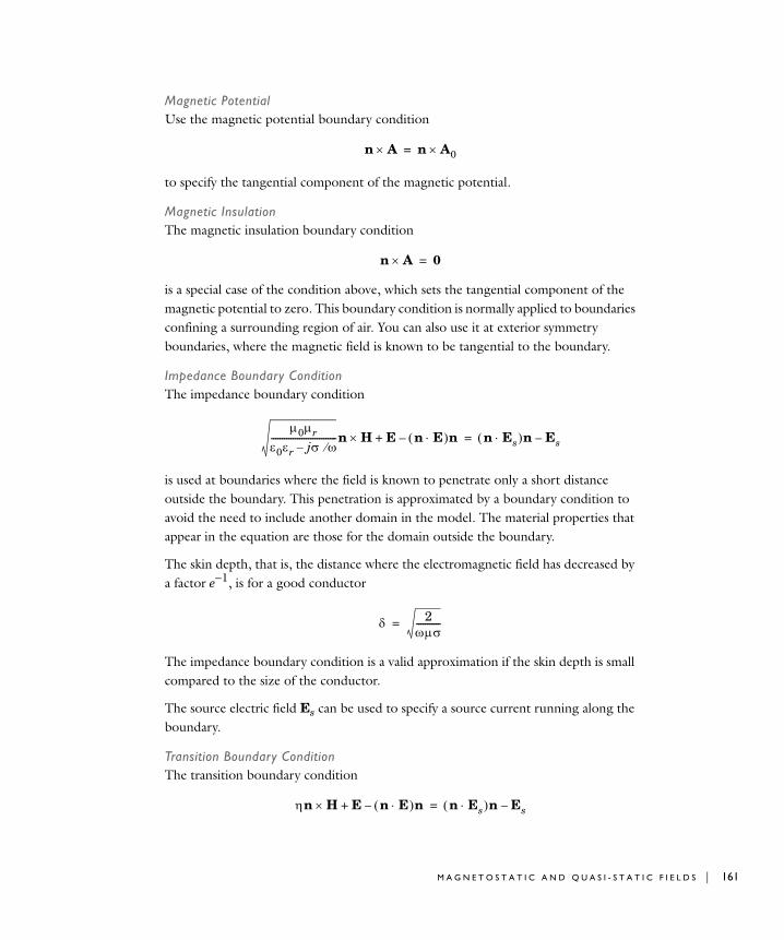
Magnetic PotentialUse the magnetic potential boundary condition
to specify the tangential component of the magnetic potential.
Magnetic InsulationThe magnetic insulation boundary condition
is a special case of the condition above, which sets the tangential component of the magnetic potential to zero. This boundary condition is normally applied to boundaries confining a surrounding region of air. You can also use it at exterior symmetry boundaries, where the magnetic field is known to be tangential to the boundary.
Impedance Boundary ConditionThe impedance boundary condition
is used at boundaries where the field is known to penetrate only a short distance outside the boundary. This penetration is approximated by a boundary condition to avoid the need to include another domain in the model. The material properties that appear in the equation are those for the domain outside the boundary.
The skin depth, that is, the distance where the electromagnetic field has decreased by a factor e−1, is for a good conductor
The impedance boundary condition is a valid approximation if the skin depth is small compared to the size of the conductor.
The source electric field Es can be used to specify a source current running along the boundary.
Transition Boundary ConditionThe transition boundary condition
n A× n A0×=
n A× 0=
µ0µrε0εr jσ ω⁄–------------------------------n H E n E⋅( )n–+× n Es⋅( )n Es–=
δ 2ωµσ-----------=
ηn H E n E⋅( )n–+× n Es⋅( )n Es–=
M A G N E T O S T A T I C A N D Q U A S I - S T A T I C F I E L D S | 161
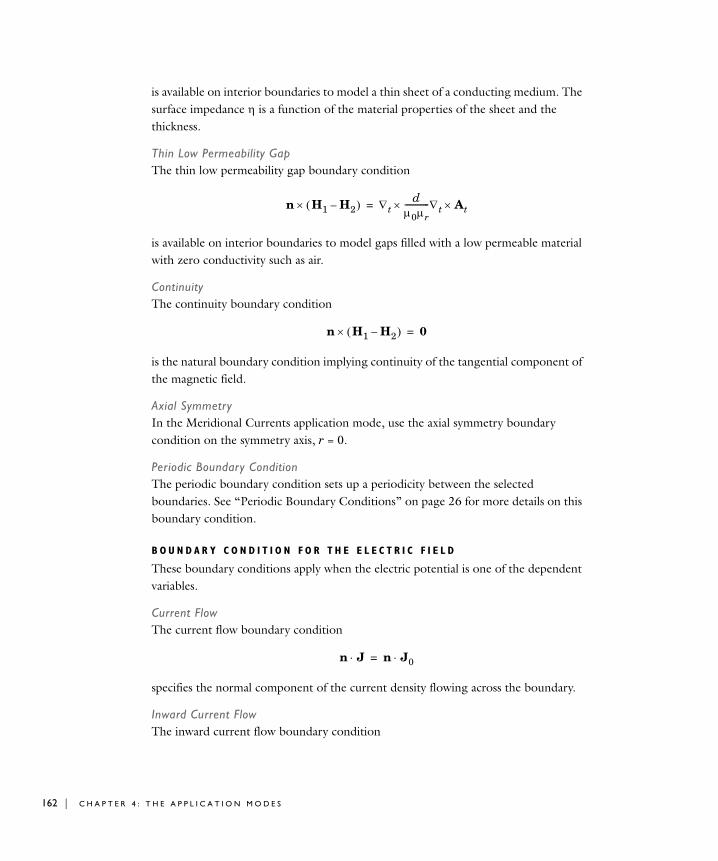
162 | C H A P T E R
is available on interior boundaries to model a thin sheet of a conducting medium. The surface impedance η is a function of the material properties of the sheet and the thickness.
Thin Low Permeability GapThe thin low permeability gap boundary condition
is available on interior boundaries to model gaps filled with a low permeable material with zero conductivity such as air.
ContinuityThe continuity boundary condition
is the natural boundary condition implying continuity of the tangential component of the magnetic field.
Axial SymmetryIn the Meridional Currents application mode, use the axial symmetry boundary condition on the symmetry axis, r = 0.
Periodic Boundary ConditionThe periodic boundary condition sets up a periodicity between the selected boundaries. See “Periodic Boundary Conditions” on page 26 for more details on this boundary condition.
B O U N D A R Y C O N D I T I O N F O R T H E E L E C T R I C F I E L D
These boundary conditions apply when the electric potential is one of the dependent variables.
Current FlowThe current flow boundary condition
specifies the normal component of the current density flowing across the boundary.
Inward Current FlowThe inward current flow boundary condition
n H1 H2–( )× ∇td
µ0µr------------∇t At××=
n H1 H2–( )× 0=
n J⋅ n J0⋅=
4 : T H E A P P L I C A T I O N M O D E S
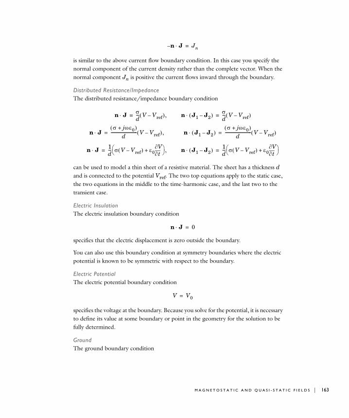
is similar to the above current flow boundary condition. In this case you specify the normal component of the current density rather than the complete vector. When the normal component Jn is positive the current flows inward through the boundary.
Distributed Resistance/ImpedanceThe distributed resistance/impedance boundary condition
can be used to model a thin sheet of a resistive material. The sheet has a thickness d and is connected to the potential Vref. The two top equations apply to the static case, the two equations in the middle to the time-harmonic case, and the last two to the transient case.
Electric InsulationThe electric insulation boundary condition
specifies that the electric displacement is zero outside the boundary.
You can also use this boundary condition at symmetry boundaries where the electric potential is known to be symmetric with respect to the boundary.
Electric PotentialThe electric potential boundary condition
specifies the voltage at the boundary. Because you solve for the potential, it is necessary to define its value at some boundary or point in the geometry for the solution to be fully determined.
GroundThe ground boundary condition
n J⋅– Jn=
n J⋅ σd--- V Vref–( ),= n J1 J2–( )⋅ σ
d--- V Vref–( )=
n J⋅σ jωε0+( )
d--------------------------- V Vref–( ),=
n J⋅ 1d--- σ V Vref–( ) ε0 t∂
∂V+⎝ ⎠
⎛ ⎞ ,=
n J1 J2–( )⋅σ jωε0+( )
d--------------------------- V Vref–( )=
n J1 J2–( )⋅ 1d--- σ V Vref–( ) ε0 t∂
∂V+⎝ ⎠
⎛ ⎞=
n J⋅ 0=
V V0=
M A G N E T O S T A T I C A N D Q U A S I - S T A T I C F I E L D S | 163
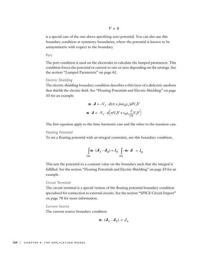
164 | C H A P T E R
is a special case of the one above specifying zero potential. You can also use this boundary condition at symmetry boundaries, where the potential is known to be antisymmetric with respect to the boundary.
Port
The port condition is used on the electrodes to calculate the lumped parameters. This condition forces the potential or current to one or zero depending on the settings. See the section “Lumped Parameters” on page 61.
Electric ShieldingThe electric shielding boundary condition describes a thin layer of a dielectric medium that shields the electric field. See “Floating Potentials and Electric Shielding” on page 33 for an example.
The first equation apply to the time-harmonic case and the other to the transient case.
Floating PotentialTo set a floating potential with an integral constraint, use this boundary condition.
This sets the potential to a constant value on the boundary such that the integral is fulfilled. See the section “Floating Potentials and Electric Shielding” on page 33 for an example.
Circuit TerminalThe circuit terminal is a special version of the floating potential boundary condition specialized for connection to external circuits. See the section “SPICE Circuit Import” on page 70 for more information.
Current SourceThe current source boundary condition
V 0=
n J ∇– t= d σ jωε0εr+( )d Vt∇⋅ ⋅
n J ∇–=⋅ t d σ Vt∇ ε0εr t∂∂ Vt∇+⎝ ⎠
⎛ ⎞⋅
n J1 J2–( )⋅Ω∂∫ I0= n J⋅–
Ω∂∫ I0=
n J1 J2–( )⋅ Jn=
4 : T H E A P P L I C A T I O N M O D E S
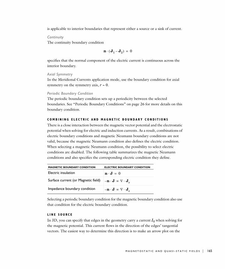
is applicable to interior boundaries that represent either a source or a sink of current.
ContinuityThe continuity boundary condition
specifies that the normal component of the electric current is continuous across the interior boundary.
Axial SymmetryIn the Meridional Currents application mode, use the boundary condition for axial symmetry on the symmetry axis, r = 0.
Periodic Boundary ConditionThe periodic boundary condition sets up a periodicity between the selected boundaries. See “Periodic Boundary Conditions” on page 26 for more details on this boundary condition.
C O M B I N I N G E L E C T R I C A N D M A G N E T I C B O U N D A R Y C O N D I T I O N S
There is a close interaction between the magnetic vector potential and the electrostatic potential when solving for electric and induction currents. As a result, combinations of electric boundary conditions and magnetic Neumann boundary conditions are not valid, because the magnetic Neumann condition also defines the electric condition. When selecting a magnetic Neumann condition, the possibility to select electric conditions are disabled. The following table summarizes the magnetic Neumann conditions and also specifies the corresponding electric condition they define.
Selecting a periodic boundary condition for the magnetic boundary condition also use that condition for the electric boundary condition.
L I N E S O U R C E
In 3D, you can specify that edges in the geometry carry a current I0 when solving for the magnetic potential. This current flows in the direction of the edges’ tangential vectors. The easiest way to determine this direction is to make an arrow plot on the
MAGNETIC BOUNDARY CONDITION ELECTRIC BOUNDARY CONDITION
Electric insulation
Surface current (or Magnetic field)
Impedance boundary condition
n J1 J2–( )⋅ 0=
n J⋅ 0=
n– J⋅ ∇ Js⋅=
n– J⋅ ∇ Js⋅=
M A G N E T O S T A T I C A N D Q U A S I - S T A T I C F I E L D S | 165
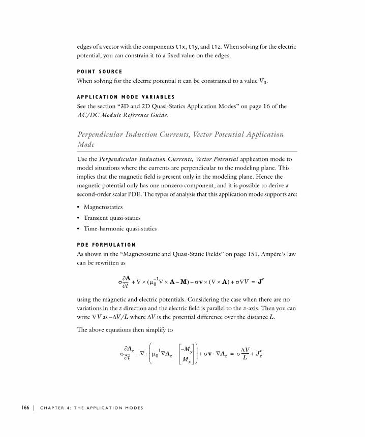
166 | C H A P T E R
edges of a vector with the components t1x, t1y, and t1z. When solving for the electric potential, you can constrain it to a fixed value on the edges.
PO I N T S O U R C E
When solving for the electric potential it can be constrained to a value V0.
A P P L I C A T I O N M O D E V A R I A B L E S
See the section “3D and 2D Quasi-Statics Application Modes” on page 16 of the AC/DC Module Reference Guide.
Perpendicular Induction Currents, Vector Potential Application Mode
Use the Perpendicular Induction Currents, Vector Potential application mode to model situations where the currents are perpendicular to the modeling plane. This implies that the magnetic field is present only in the modeling plane. Hence the magnetic potential only has one nonzero component, and it is possible to derive a second-order scalar PDE. The types of analysis that this application mode supports are:
• Magnetostatics
• Transient quasi-statics
• Time-harmonic quasi-statics
P D E F O R M U L A T I O N
As shown in the “Magnetostatic and Quasi-Static Fields” on page 151, Ampère’s law can be rewritten as
using the magnetic and electric potentials. Considering the case when there are no variations in the z direction and the electric field is parallel to the z-axis. Then you can write as −∆V/L where ∆V is the potential difference over the distance L.
The above equations then simplify to
σt∂
∂A ∇ µ01– ∇ A× M–( )× σv ∇ A×( ) σ V∇+×–+ Je
=
∇V
σt∂
∂Az ∇ µ01– Az∇
M– y
Mx
–⎝ ⎠⎜ ⎟⎜ ⎟⎛ ⎞
⋅– σv Az∇⋅+ σ∆VL
-------- Jze
+=
4 : T H E A P P L I C A T I O N M O D E S
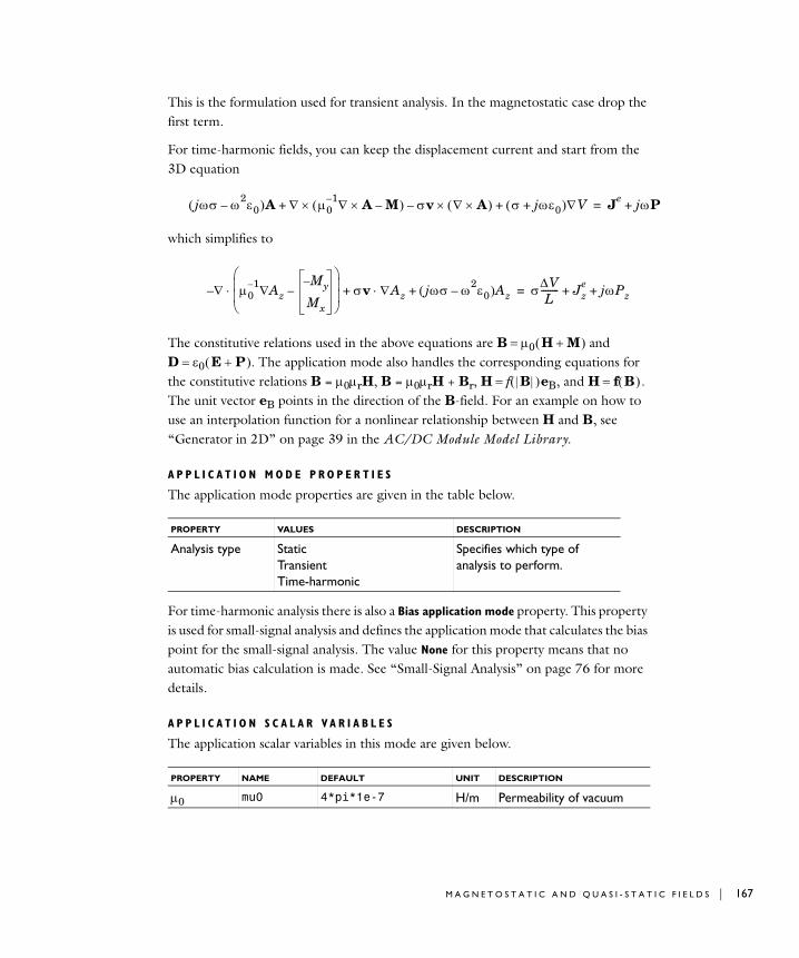
This is the formulation used for transient analysis. In the magnetostatic case drop the first term.
For time-harmonic fields, you can keep the displacement current and start from the 3D equation
which simplifies to
The constitutive relations used in the above equations are B = µ0 ( H + M ) and D = ε0 ( E + P ). The application mode also handles the corresponding equations for the constitutive relations B = µ0µrH, B = µ0µrH + Br, H = f( | B | ) eB, and H = f( B ) . The unit vector eB points in the direction of the B-field. For an example on how to use an interpolation function for a nonlinear relationship between H and B, see “Generator in 2D” on page 39 in the AC/DC Module Model Library.
A P P L I C A T I O N M O D E P R O P E R T I E S
The application mode properties are given in the table below.
For time-harmonic analysis there is also a Bias application mode property. This property is used for small-signal analysis and defines the application mode that calculates the bias point for the small-signal analysis. The value None for this property means that no automatic bias calculation is made. See “Small-Signal Analysis” on page 76 for more details.
A P P L I C A T I O N S C A L A R V A R I A B L E S
The application scalar variables in this mode are given below.
PROPERTY VALUES DESCRIPTION
Analysis type Static Transient Time-harmonic
Specifies which type of analysis to perform.
PROPERTY NAME DEFAULT UNIT DESCRIPTION
µ0 mu0 4*pi*1e-7 H/m Permeability of vacuum
jωσ ω2ε0–( )A ∇ µ01– ∇ A M–×( )× σv ∇ A×( ) σ jωε0+( )∇V+×–+ Je jωP+=
∇– µ01– Az∇
M– y
Mx
–⎝ ⎠⎜ ⎟⎜ ⎟⎛ ⎞
⋅ σv+ ∇Az⋅ jωσ ω2ε0–( )Az+ σ∆VL
-------- Jze
+ jωPz+=
M A G N E T O S T A T I C A N D Q U A S I - S T A T I C F I E L D S | 167
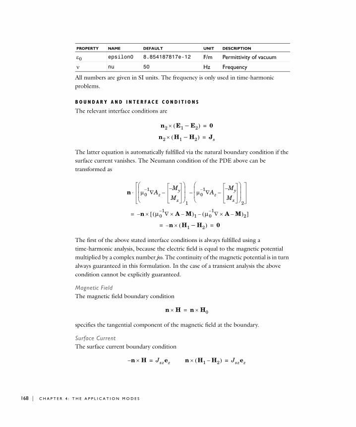
168 | C H A P T E R
All numbers are given in SI units. The frequency is only used in time-harmonic problems.
B O U N D A R Y A N D I N T E R F A C E C O N D I T I O N S
The relevant interface conditions are
The latter equation is automatically fulfilled via the natural boundary condition if the surface current vanishes. The Neumann condition of the PDE above can be transformed as
The first of the above stated interface conditions is always fulfilled using a time-harmonic analysis, because the electric field is equal to the magnetic potential multiplied by a complex number jω. The continuity of the magnetic potential is in turn always guaranteed in this formulation. In the case of a transient analysis the above condition cannot be explicitly guaranteed.
Magnetic FieldThe magnetic field boundary condition
specifies the tangential component of the magnetic field at the boundary.
Surface CurrentThe surface current boundary condition
ε0 epsilon0 8.854187817e-12 F/m Permittivity of vacuum
ν nu 50 Hz Frequency
PROPERTY NAME DEFAULT UNIT DESCRIPTION
n2 E1 E2–( )× 0=
n2 H1 H2–( )× Js=
n µ01– Az∇
M– y
Mx
–⎝ ⎠⎜ ⎟⎜ ⎟⎛ ⎞
1
µ01– Az∇
M– y
Mx
–⎝ ⎠⎜ ⎟⎜ ⎟⎛ ⎞
2
–⋅
n µ01– ∇ A× M–( )1 µ0
1– ∇ A× M–( )2–[ ]×–=
n H1 H2–( )×– 0= =
n H× n H0×=
n H×– Jszez= n H1 H2–( )× Jszez=
4 : T H E A P P L I C A T I O N M O D E S
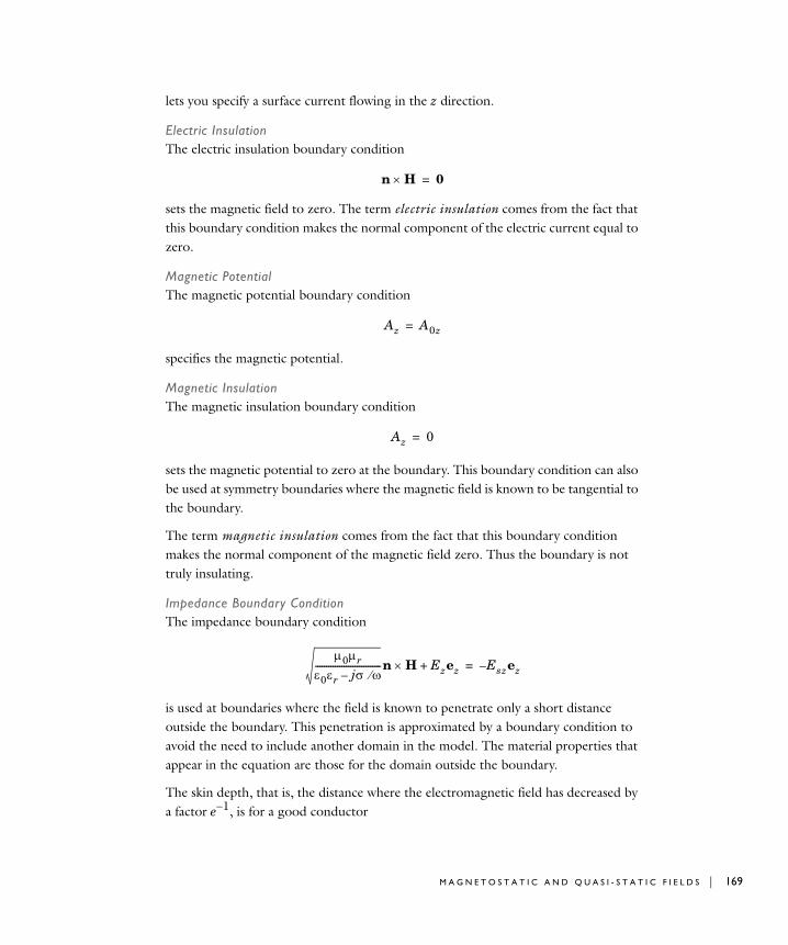
lets you specify a surface current flowing in the z direction.
Electric InsulationThe electric insulation boundary condition
sets the magnetic field to zero. The term electric insulation comes from the fact that this boundary condition makes the normal component of the electric current equal to zero.
Magnetic PotentialThe magnetic potential boundary condition
specifies the magnetic potential.
Magnetic InsulationThe magnetic insulation boundary condition
sets the magnetic potential to zero at the boundary. This boundary condition can also be used at symmetry boundaries where the magnetic field is known to be tangential to the boundary.
The term magnetic insulation comes from the fact that this boundary condition makes the normal component of the magnetic field zero. Thus the boundary is not truly insulating.
Impedance Boundary ConditionThe impedance boundary condition
is used at boundaries where the field is known to penetrate only a short distance outside the boundary. This penetration is approximated by a boundary condition to avoid the need to include another domain in the model. The material properties that appear in the equation are those for the domain outside the boundary.
The skin depth, that is, the distance where the electromagnetic field has decreased by a factor e−1, is for a good conductor
n H× 0=
Az A0z=
Az 0=
µ0µr
ε0εr jσ ω⁄–------------------------------n H Ezez+× Eszez–=
M A G N E T O S T A T I C A N D Q U A S I - S T A T I C F I E L D S | 169
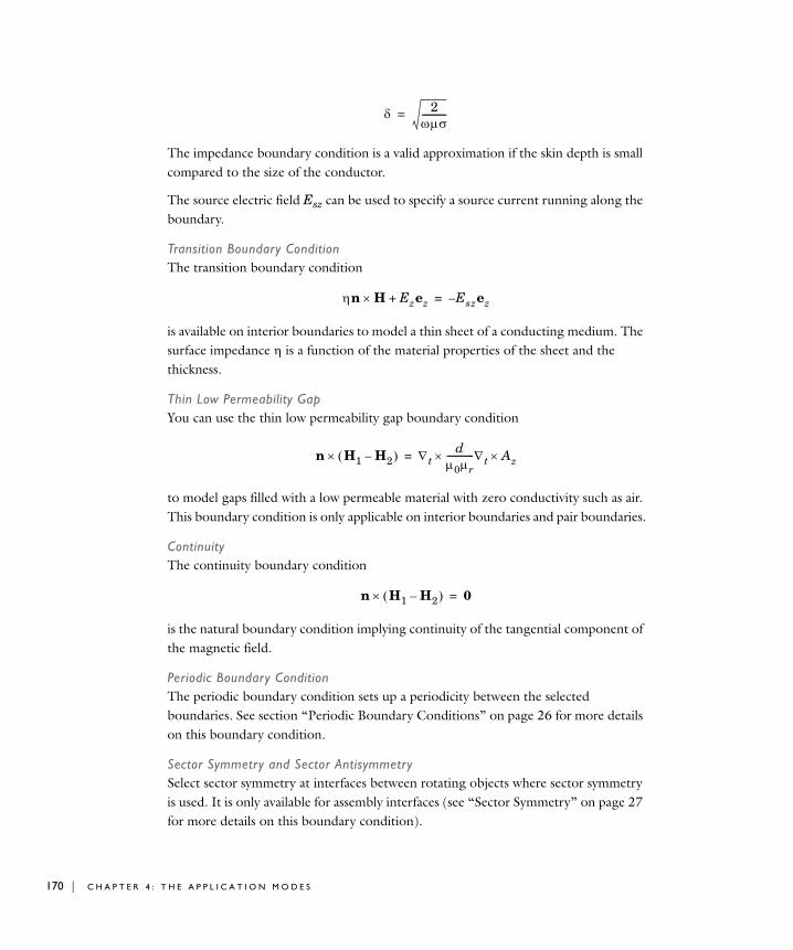
170 | C H A P T E R
The impedance boundary condition is a valid approximation if the skin depth is small compared to the size of the conductor.
The source electric field Esz can be used to specify a source current running along the boundary.
Transition Boundary ConditionThe transition boundary condition
is available on interior boundaries to model a thin sheet of a conducting medium. The surface impedance η is a function of the material properties of the sheet and the thickness.
Thin Low Permeability GapYou can use the thin low permeability gap boundary condition
to model gaps filled with a low permeable material with zero conductivity such as air. This boundary condition is only applicable on interior boundaries and pair boundaries.
ContinuityThe continuity boundary condition
is the natural boundary condition implying continuity of the tangential component of the magnetic field.
Periodic Boundary ConditionThe periodic boundary condition sets up a periodicity between the selected boundaries. See section “Periodic Boundary Conditions” on page 26 for more details on this boundary condition.
Sector Symmetry and Sector AntisymmetrySelect sector symmetry at interfaces between rotating objects where sector symmetry is used. It is only available for assembly interfaces (see “Sector Symmetry” on page 27 for more details on this boundary condition).
δ 2ωµσ-----------=
ηn H Ezez+× Eszez–=
n H1 H2–( )× ∇td
µ0µr------------∇t Az××=
n H1 H2–( )× 0=
4 : T H E A P P L I C A T I O N M O D E S
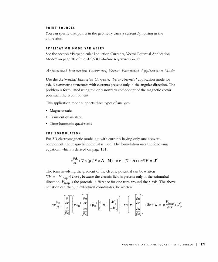
PO I N T S O U R C E S
You can specify that points in the geometry carry a current I0 flowing in the z direction.
A P P L I C A T I O N M O D E VA R I A B L E S
See the section “Perpendicular Induction Currents, Vector Potential Application Mode” on page 30 of the AC/DC Module Reference Guide.
Azimuthal Induction Currents, Vector Potential Application Mode
Use the Azimuthal Induction Currents, Vector Potential application mode for axially symmetric structures with currents present only in the angular direction. The problem is formulated using the only nonzero component of the magnetic vector potential, the component.
This application mode supports three types of analyses:
• Magnetostatic
• Transient quasi-static
• Time-harmonic quasi-static
P D E F O R M U L A T I O N
For 2D electromagnetic modeling, with currents having only one nonzero component, the magnetic potential is used. The formulation uses the following equation, which is derived on page 151.
The term involving the gradient of the electric potential can be written , because the electric field is present only in the azimuthal
direction. Vloop is the potential difference for one turn around the z-axis. The above equation can then, in cylindrical coordinates, be written
ϕ
σt∂
∂A ∇ µ01– ∇ A× M–( )× σv ∇ A×( ) σ V∇+×–+ Je
=
V∇ Vloop 2πr( )⁄–=
σrt∂
∂u r∂∂
z∂∂
T
rµ01– r∂
∂u
z∂∂u
µ01– 2
0u
Mz
M– r
–+
⎝ ⎠⎜ ⎟⎜ ⎟⎜ ⎟⎜ ⎟⎛ ⎞
– rσ v r∂∂u
z∂∂u
⋅
⎝ ⎠⎜ ⎟⎜ ⎟⎜ ⎟⎜ ⎟⎛ ⎞
2σvru+ + σVloop2πr------------- Jϕ
e+=
M A G N E T O S T A T I C A N D Q U A S I - S T A T I C F I E L D S | 171
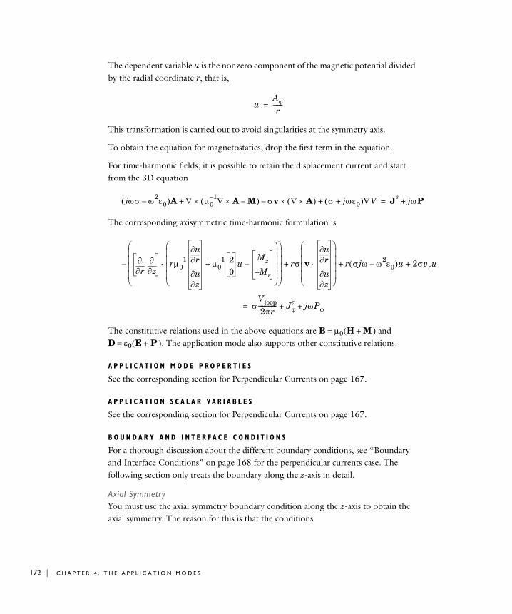
172 | C H A P T E R
ru
The dependent variable u is the nonzero component of the magnetic potential divided by the radial coordinate r, that is,
This transformation is carried out to avoid singularities at the symmetry axis.
To obtain the equation for magnetostatics, drop the first term in the equation.
For time-harmonic fields, it is possible to retain the displacement current and start from the 3D equation
The corresponding axisymmetric time-harmonic formulation is
The constitutive relations used in the above equations are B = µ0 (H + M ) and D = ε0 (E + P ). The application mode also supports other constitutive relations.
A P P L I C A T I O N M O D E P R O P E R T I E S
See the corresponding section for Perpendicular Currents on page 167.
A P P L I C A T I O N S C A L A R V A R I A B L E S
See the corresponding section for Perpendicular Currents on page 167.
B O U N D A R Y A N D I N T E R F A C E C O N D I T I O N S
For a thorough discussion about the different boundary conditions, see “Boundary and Interface Conditions” on page 168 for the perpendicular currents case. The following section only treats the boundary along the z-axis in detail.
Axial SymmetryYou must use the axial symmetry boundary condition along the z-axis to obtain the axial symmetry. The reason for this is that the conditions
uAϕr
-------=
jωσ ω2ε0–( )A ∇ µ01– ∇ A M–×( )× σv ∇ A×( ) σ jωε0+( )∇V+×–+ Je jωP+=
r∂∂
z∂∂ rµ0
1– r∂∂u
z∂∂u
µ01– 2
0u
Mz
M– r
–+
⎝ ⎠⎜ ⎟⎜ ⎟⎜ ⎟⎜ ⎟⎛ ⎞
⋅
⎝ ⎠⎜ ⎟⎜ ⎟⎜ ⎟⎜ ⎟⎛ ⎞
– rσ v r∂∂u
z∂∂u
⋅
⎝ ⎠⎜ ⎟⎜ ⎟⎜ ⎟⎜ ⎟⎛ ⎞
r σjω ω2ε0–( )u 2σv+ + +
σVloop2πr------------- Jϕ
e+ jωPϕ+=
4 : T H E A P P L I C A T I O N M O D E S
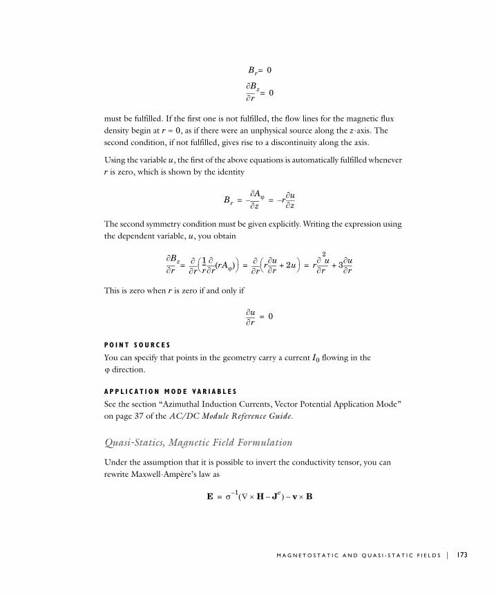
must be fulfilled. If the first one is not fulfilled, the flow lines for the magnetic flux density begin at r = 0, as if there were an unphysical source along the z-axis. The second condition, if not fulfilled, gives rise to a discontinuity along the axis.
Using the variable u, the first of the above equations is automatically fulfilled whenever r is zero, which is shown by the identity
The second symmetry condition must be given explicitly. Writing the expression using the dependent variable, u, you obtain
This is zero when r is zero if and only if
PO I N T S O U R C E S
You can specify that points in the geometry carry a current I0 flowing in the direction.
A P P L I C A T I O N M O D E VA R I A B L E S
See the section “Azimuthal Induction Currents, Vector Potential Application Mode” on page 37 of the AC/DC Module Reference Guide.
Quasi-Statics, Magnetic Field Formulation
Under the assumption that it is possible to invert the conductivity tensor, you can rewrite Maxwell-Ampère’s law as
Br 0=
r∂∂Bz 0=
Br z∂∂Aϕ– r
z∂∂u
–= =
r∂∂Bz
r∂∂ 1
r---
r∂∂ rAϕ( )⎝ ⎠
⎛ ⎞=r∂
∂ rr∂
∂u 2u+⎝ ⎠⎛ ⎞ r
r
2
∂∂ u 3
r∂∂u
+= =
r∂∂u 0=
ϕ
E σ 1– ∇ H× Je–( ) v B×–=
M A G N E T O S T A T I C A N D Q U A S I - S T A T I C F I E L D S | 173
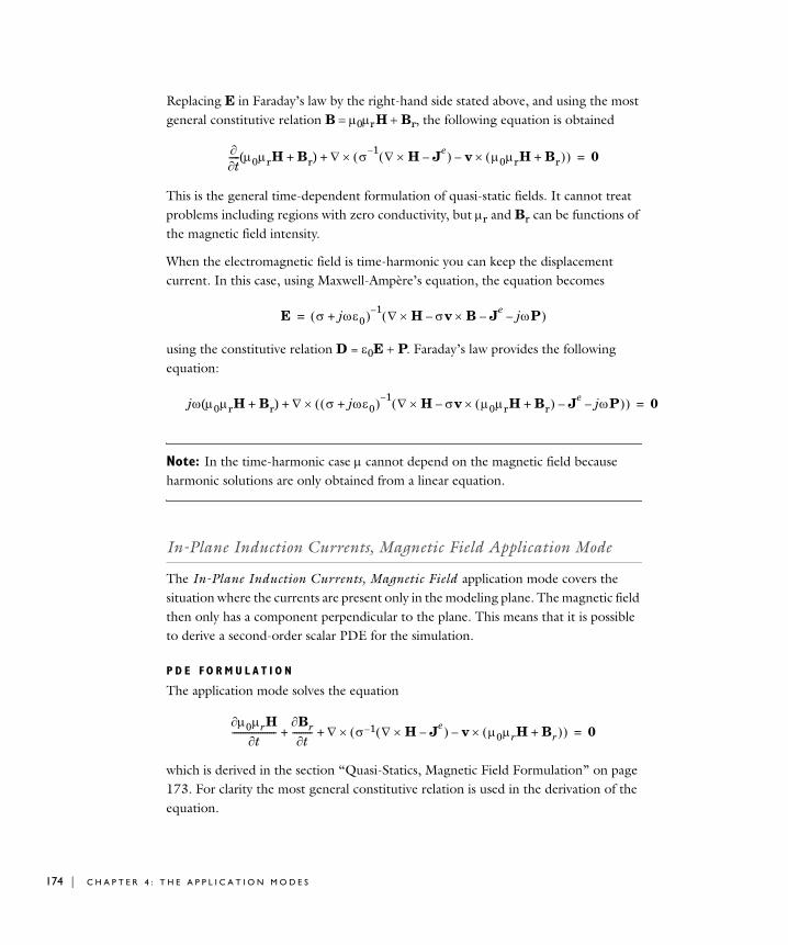
174 | C H A P T E R
Replacing E in Faraday’s law by the right-hand side stated above, and using the most general constitutive relation B = µ0µr H + Br, the following equation is obtained
This is the general time-dependent formulation of quasi-static fields. It cannot treat problems including regions with zero conductivity, but µr and Br can be functions of the magnetic field intensity.
When the electromagnetic field is time-harmonic you can keep the displacement current. In this case, using Maxwell-Ampère’s equation, the equation becomes
using the constitutive relation D = ε0E + P. Faraday’s law provides the following equation:
Note: In the time-harmonic case µ cannot depend on the magnetic field because harmonic solutions are only obtained from a linear equation.
In-Plane Induction Currents, Magnetic Field Application Mode
The In-Plane Induction Currents, Magnetic Field application mode covers the situation where the currents are present only in the modeling plane. The magnetic field then only has a component perpendicular to the plane. This means that it is possible to derive a second-order scalar PDE for the simulation.
P D E F O R M U L A T I O N
The application mode solves the equation
which is derived in the section “Quasi-Statics, Magnetic Field Formulation” on page 173. For clarity the most general constitutive relation is used in the derivation of the equation.
∂t∂
----- µ0µrH Br+( ) ∇ σ 1– ∇ H× Je–( ) v µ0µrH Br+( )×–( )×+ 0=
E σ jωε0+( ) 1– ∇ H× σv B×– Je– jωP–( )=
jω µ0µrH Br+( ) ∇ σ jωε0+( ) 1– ∇ H× σv µ0µrH Br+( )×– Je– jωP–( )( )×+ 0=
µ0µrH∂t∂
--------------------Br∂t∂
--------- ∇ σ 1– ∇ H× Je–( ) v µ0µrH Br+( )×–( )×+ + 0=
4 : T H E A P P L I C A T I O N M O D E S
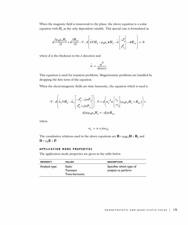
When the magnetic field is transversal to the plane, the above equation is a scalar equation with Hz as the only dependent variable. This special case is formulated as
where d is the thickness in the z direction and
This equation is used for transient problems. Magnetostatic problems are handled by dropping the first term of the equation.
When the electromagnetic fields are time-harmonic, the equation which is used is
where
The constitutive relations used in the above equations are B = µ0µr H + Br and D = ε0 E + P.
A P P L I C A T I O N M O D E P R O P E R T I E S
The application mode properties are given in the table below.
PROPERTY VALUES DESCRIPTION
Analysis type Static Transient Time-harmonic
Specifies which type of analysis to perform
dµ0µrHz∂
t∂----------------------- d
Brz∂t∂
------------ ∇ d σ Hz∇ µ0µrvHz– σJy
e–
Jxe
– vBrz–
⎝ ⎠⎜ ⎟⎜ ⎟⎜ ⎟⎛ ⎞
⋅–+ 0=
σ σT
det σ( )----------------=
∇ d σc Hz∇ σcJy
e– jωPy–
Jxe jωPx+
–
⎝ ⎠⎜ ⎟⎜ ⎟⎜ ⎟⎛ ⎞
∇ d σc1– σ
vy
vx–µ0µrHz Brz+( )
⎝ ⎠⎜ ⎟⎜ ⎟⎛ ⎞
+×–⋅–
djωµ0µrHz djωBrz–=
σc σ jωε0+=
M A G N E T O S T A T I C A N D Q U A S I - S T A T I C F I E L D S | 175
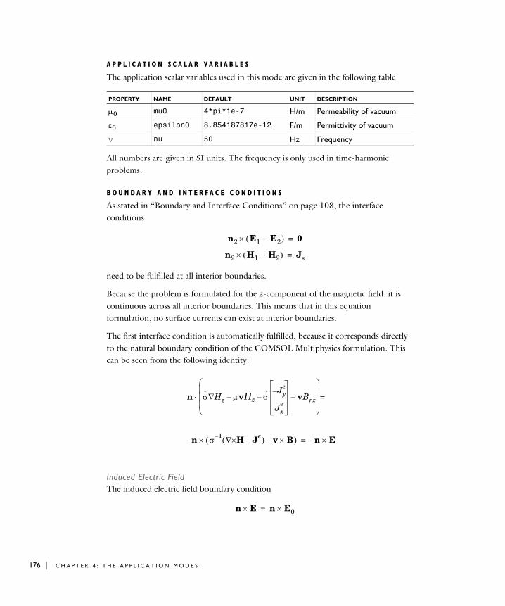
176 | C H A P T E R
A P P L I C A T I O N S C A L A R V A R I A B L E S
The application scalar variables used in this mode are given in the following table.
All numbers are given in SI units. The frequency is only used in time-harmonic problems.
B O U N D A R Y A N D I N T E R F A C E C O N D I T I O N S
As stated in “Boundary and Interface Conditions” on page 108, the interface conditions
need to be fulfilled at all interior boundaries.
Because the problem is formulated for the z-component of the magnetic field, it is continuous across all interior boundaries. This means that in this equation formulation, no surface currents can exist at interior boundaries.
The first interface condition is automatically fulfilled, because it corresponds directly to the natural boundary condition of the COMSOL Multiphysics formulation. This can be seen from the following identity:
Induced Electric FieldThe induced electric field boundary condition
PROPERTY NAME DEFAULT UNIT DESCRIPTION
µ0 mu0 4*pi*1e-7 H/m Permeability of vacuum
ε0 epsilon0 8.854187817e-12 F/m Permittivity of vacuum
ν nu 50 Hz Frequency
n2 E1 E2–( )× 0=
n2 H1 H2–( )× Js=
n σ Hz∇ µvHz– σJy
e–
Jxe
– vBrz–
⎝ ⎠⎜ ⎟⎜ ⎟⎜ ⎟⎛ ⎞
n– σ 1– H∇× Je–( ) v B×–( )×
=⋅
n E×–=
n E× n E0×=
4 : T H E A P P L I C A T I O N M O D E S
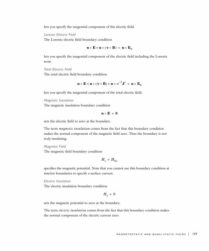
lets you specify the tangential component of the electric field.
Lorentz Electric FieldThe Lorentz electric field boundary condition
lets you specify the tangential component of the electric field including the Lorentz term.
Total Electric FieldThe total electric field boundary condition
lets you specify the tangential component of the total electric field.
Magnetic InsulationThe magnetic insulation boundary condition
sets the electric field to zero at the boundary.
The term magnetic insulation comes from the fact that this boundary condition makes the normal component of the magnetic field zero. Thus the boundary is not truly insulating.
Magnetic FieldThe magnetic field boundary condition
specifies the magnetic potential. Note that you cannot use this boundary condition at interior boundaries to specify a surface current.
Electric InsulationThe electric insulation boundary condition
sets the magnetic potential to zero at the boundary.
The term electric insulation comes from the fact that this boundary condition makes the normal component of the electric current zero.
n E× n v B×( )×+ n E0×=
n E n v B×( ) n σ 1– Je×+×+× n E0×=
n E× 0=
Hz H0z=
Hz 0=
M A G N E T O S T A T I C A N D Q U A S I - S T A T I C F I E L D S | 177
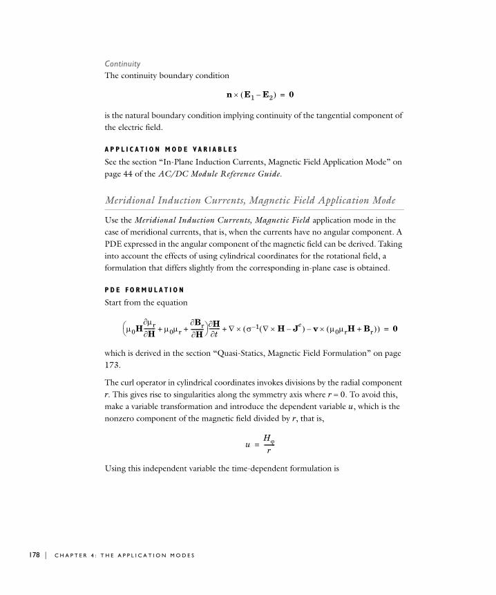
178 | C H A P T E R
ContinuityThe continuity boundary condition
is the natural boundary condition implying continuity of the tangential component of the electric field.
A P P L I C A T I O N M O D E V A R I A B L E S
See the section “In-Plane Induction Currents, Magnetic Field Application Mode” on page 44 of the AC/DC Module Reference Guide.
Meridional Induction Currents, Magnetic Field Application Mode
Use the Meridional Induction Currents, Magnetic Field application mode in the case of meridional currents, that is, when the currents have no angular component. A PDE expressed in the angular component of the magnetic field can be derived. Taking into account the effects of using cylindrical coordinates for the rotational field, a formulation that differs slightly from the corresponding in-plane case is obtained.
P D E F O R M U L A T I O N
Start from the equation
which is derived in the section “Quasi-Statics, Magnetic Field Formulation” on page 173.
The curl operator in cylindrical coordinates invokes divisions by the radial component r. This gives rise to singularities along the symmetry axis where r = 0. To avoid this, make a variable transformation and introduce the dependent variable u, which is the nonzero component of the magnetic field divided by r, that is,
Using this independent variable the time-dependent formulation is
n E1 E2–( )× 0=
µ0Hµr∂H∂
-------- µ0µrBr∂H∂
---------+ +⎝ ⎠⎛ ⎞ H∂
t∂-------- ∇ σ 1– ∇ H× Je
–( ) v µ0µrH Br+( )×–( )×+ 0=
uHϕr
--------=
4 : T H E A P P L I C A T I O N M O D E S
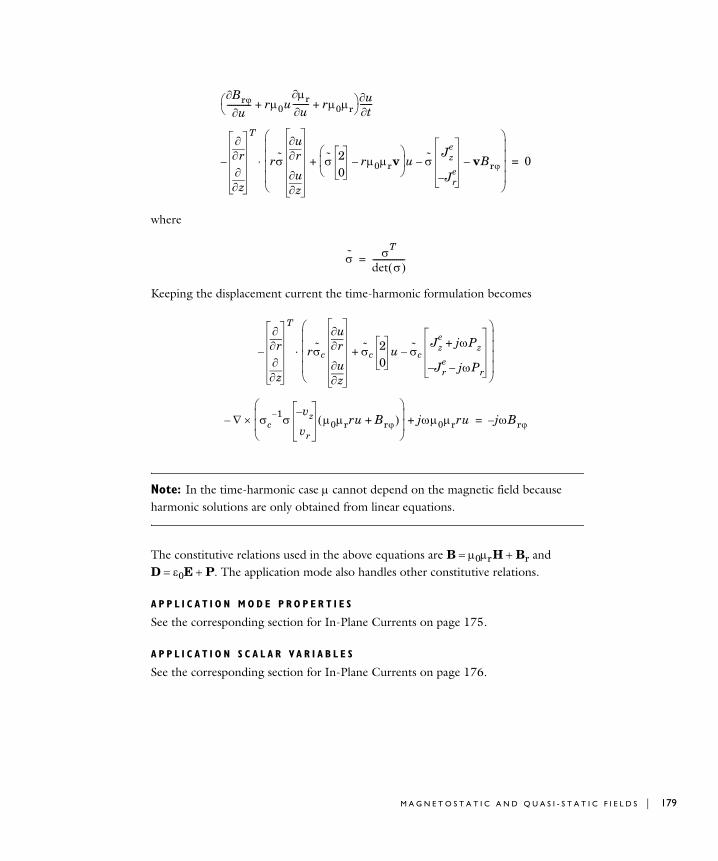
where
Keeping the displacement current the time-harmonic formulation becomes
Note: In the time-harmonic case µ cannot depend on the magnetic field because harmonic solutions are only obtained from linear equations.
The constitutive relations used in the above equations are B = µ0µr H + Br and D = ε0E + P . The application mode also handles other constitutive relations.
A P P L I C A T I O N M O D E P R O P E R T I E S
See the corresponding section for In-Plane Currents on page 175.
A P P L I C A T I O N S C A L A R V A R I A B L E S
See the corresponding section for In-Plane Currents on page 176.
Brϕ∂u∂
------------ rµ0uµr∂u∂
-------- rµ0µr+ +⎝ ⎠⎛ ⎞ u∂
t∂------
r∂∂
z∂∂
T
rσ r∂∂u
z∂∂u
σ 20
rµ0µrv–⎝ ⎠⎜ ⎟⎛ ⎞
u σJz
e
J– re
– vBrϕ–+
⎝ ⎠⎜ ⎟⎜ ⎟⎜ ⎟⎜ ⎟⎛ ⎞
⋅– 0=
σ σT
det σ( )----------------=
r∂∂
z∂∂
T
– rσcr∂
∂u
z∂∂u
σc20
u σcJz
e jωPz+
J– re jωPr–
–+
⎝ ⎠⎜ ⎟⎜ ⎟⎜ ⎟⎜ ⎟⎛ ⎞
⋅
∇ σc1– σ
vz–
vr
µ0µrru Brϕ+( )⎝ ⎠⎜ ⎟⎜ ⎟⎛ ⎞
×– jωµ0µrru+ jωBrϕ–=
M A G N E T O S T A T I C A N D Q U A S I - S T A T I C F I E L D S | 179
180 | C H A P T E R
B O U N D A R Y A N D I N T E R F A C E C O N D I T I O N S
For a thorough discussion on the different boundary conditions, see “Boundary and Interface Conditions” on page 176 for the in-plane case. This section only covers the boundary along the z-axis in detail.
Axial SymmetryYou must use the axial symmetry boundary condition along the z axis to obtain the axial symmetry. The reason for this is that the conditions
must be fulfilled. If the first one is not fulfilled, the flow lines for the current flow begin at r = 0, as if there were a nonphysical source along the z-axis. If the second condition is not fulfilled, it gives rise to a discontinuity along the axis.
Using the variable u, the first of the above equations is automatically fulfilled whenever r is zero, which is shown by the identity
The second symmetry condition must be given explicitly. Writing the expression using the dependent variable, u, the equation for the symmetry condition becomes
This is zero when r is zero if and only if
A P P L I C A T I O N M O D E V A R I A B L E S
See the section “Meridional Induction Currents, Magnetic Field Application Mode” on page 50 of the AC/DC Module Reference Guide.
Jr 0=
r∂∂Jz 0=
Jr z∂∂Hϕ– r
z∂∂u
–= =
r∂∂Jz
r∂∂ 1
r---
r∂∂ rHϕ( )⎝ ⎠
⎛ ⎞=r∂
∂ rr∂
∂u 2u+⎝ ⎠⎛ ⎞ r
r
2
∂∂ u 3
r∂∂u
+= =
r∂∂u 0=
4 : T H E A P P L I C A T I O N M O D E S
Magnetostatics Without Currents
In magnetostatic problems where no electric currents are present, the problem can be solved using a scalar magnetic potential. In a current-free region you have
This implies that you can define the magnetic scalar potential Vm from the relation
This is analogous to the definition of the electric potential for static electric fields.
Using the constitutive relation B = µ0 ( H + M ) the equation
becomes
Magnetostatics, No Currents Application Mode
The Magnetostatics, No Currents application mode solves the equation derived above. This equation assumes the constitutive relation B = µ0 ( H + M ). The application mode also handles the corresponding equations for the constitutive relations B = µ0µrH, B = µ0µrH + Br, B= f ( | H | ) eH, and B= f ( | H | ). The unit vector eH is directed in the same direction as the H-field.
A P P L I C A T I O N S C A L A R V A R I A B L E S
The application-specific scalar variable in this application mode is µ0:
The default value is given in SI units.
B O U N D A R Y A N D I N T E R F A C E C O N D I T I O N S
In magnetostatics the relevant boundary condition between two domains 1 and 2 is
This is automatically satisfied by the natural boundary condition, which is
PROPERTY NAME DEFAULT UNIT DESCRIPTION
µ0 mu0 4*pi*1e-7 H/m Permeability of vacuum
∇ H× 0=
H ∇Vm–=
∇ B⋅ 0=
∇– µ0∇Vm µ0M–( )⋅ 0=
n2 B1 B2–( )⋅ 0=
M A G N E T O S T A T I C A N D Q U A S I - S T A T I C F I E L D S | 181
182 | C H A P T E R
Magnetic Flux DensityThe magnetic flux density boundary condition
lets you specify the normal component of the magnetic flux density at the boundary.
Inward Flux DensityThe inward flux density boundary condition
is similar to magnetic flux density boundary condition. The inward flux density boundary condition lets you specify the normal component of the magnetic flux density as a scalar. A positive value indicates an inward flux.
Magnetic InsulationThe magnetic insulation boundary condition
sets the normal component of the magnetic flux density to zero. This boundary condition is useful at boundaries confining a surrounding region of air.
Magnetic PotentialThe magnetic potential boundary condition
lets you specify the potential at the boundary.
Zero PotentialThe zero potential boundary condition
sets the magnetic potential to zero at the boundary.
Magnetic ShieldingThe magnetic shielding boundary condition describes a thin layer of a permeable medium which shields the magnetic field.
n µ0∇Vm M–( )1 µ0∇Vm M–( )2–[ ]⋅ n B1 B2–( )⋅– 0= =
n B⋅ n B0⋅=
n– B⋅ Bn=
n B⋅ 0=
Vm Vm0=
Vm 0=
4 : T H E A P P L I C A T I O N M O D E S
Thin Low Permeability GapYou can use the thin low permeability gap boundary condition
to model a thin gap of a low permeable material such as air. The layer has the thickness d and the relative permeability µr. This boundary condition is only available at the border between the parts in an assembly.
ContinuityThe continuity boundary condition
is the natural boundary condition ensuring continuity of the normal component of the magnetic flux density.
Periodic Boundary ConditionThe periodic boundary condition sets up a periodicity between the selected boundaries. See “Periodic Boundary Conditions” on page 26 for more details on this boundary condition.
Sector Symmetry and Sector AntisymmetrySelect sector symmetry at interfaces between rotating objects where sector symmetry is used. It is only available for assembly interfaces (see “Sector Symmetry” on page 27 for more details on this boundary condition).
PO I N T C O N D I T I O N
To obtain a unique solution, you must provide the potential at (at least) one point. If you use the magnetic insulation boundary condition everywhere, the potential has to be fixed using a point condition. With the available point condition you can set Vm = Vm0, where Vm0 is a given constant.
A P P L I C A T I O N M O D E VA R I A B L E S
See the section “Magnetostatics, No Currents Application Mode” on page 56 of the AC/DC Module Reference Guide.
n B⋅( )1µd--- Vm1 Vm2–( )=
n B⋅( )2µd--- Vm2 Vm1–( )=
n B1 B2–( )⋅ 0=
M A G N E T O S T A T I C A N D Q U A S I - S T A T I C F I E L D S | 183

184 | C H A P T E R
4 : T H E A P P L I C A T I O N M O D E S
5
G l o s s a r y
This glossary contains finite element modeling terms in an electromagnetics context. For mathematical terms as well as geometry and CAD terms specific to the COMSOL Multiphysics software and documentation, please see the glossary in the COMSOL Multiphysics User’s Guide. For references to more information about a term, see the index.
185
186 | C H A P T E R
G l o s s a r y o f T e rm sanisotropy Variation of material properties with direction.
constitutive relation The relation between the D and E fields and between the B and H fields. These relations depend on the material properties.
eddy currents Induced currents normal to a time-varying magnetic flux in a ferromagnetic material.
edge element See vector element.
electric dipole Two equal and opposite charges +q and −q separated a short distance d. The electric dipole moment is given by p = qd, where d is a vector going from −q to +q.
gauge transformation A variable transformation of the electric and magnetic potentials that leaves Maxwell’s equations invariant.
magnetic dipole A small circular loop carrying a current. The magnetic dipole moment is m = IAe, where I is the current carried by the loop, A its area, and e a unit vector along the central axis of the loop.
Nedelec’s edge element See vector element.
phasor A complex function of space representing a sinusoidally varying quantity.
quasi-static approximation The electromagnetic fields are assumed to vary slowly, so that the retardation effects can be neglected. This approximation is valid when the geometry under study is considerably smaller than the wavelength.
vector element A finite element often used for electromagnetic vector fields. The tangential component of the vector field at the mesh edges is used as a degree of freedom. Also called Nedelec’s edge element or just edge element.
5 : G L O S S A R Y
I N D E X
3D Conductive Media DC
application mode 134
3D Electrostatics
application mode 140
3D Electrostatics, Generalized
application mode 145
3D magnetostatics
application mode 154
3D quasi-statics
application mode 154
A AC/DC Material Properties library 133
AC/DC Module 3.4
new features in 5
admittance 122
Ampère’s law 102
in quasi-statics 107
analysis
static 131
time-harmonic 131
transient 131
analysis capabilities 129
analysis type 131
anisotropic material 107
antiperiodic boundaries 43
application mode 8, 128
Azimuthal currents quasi-statics 171
Conductive Media DC (3D) 134
Electrostatics 140
Electrostatics, Generalized 145
In-plane currents quasi-statics 174
Magnetostatics (3D) 154
Magnetostatics, no currents 181
Meridional currents quasi-statics 178
Perpendicular currents quasi-statics
166
Quasi-statics (3D) 154
Quasi-statics, small currents 166
Shell, Conductive Media DC 139
Small in-plane currents 166
Small meridional currents 166
application mode properties 132
application mode property
analysis type 158, 167, 175
gauge fixing 158
potentials 158
application mode variable 132
application scalar variable 25, 131, 132
Application Scalar Variables dialog box
13, 26, 131
assemblies, in electromagnetics 97
Axes/Grid Settings dialog box 23
axial symmetry 17
boundary condition 149, 172, 180
Azimuthal currents quasi-statics
application mode 171
model 22
B bias application mode 76
bipolar transistor 72
boundary condition 132
axisymmetric 149, 172, 180
distributed resistance 163
electric shielding 138, 142, 164
floating potential 137, 142
impedance 161, 169
magnetic shielding 182
transition 170
boundary conditions
for minimizing problem size 18
Boundary Settings dialog box 13, 26, 132
C capacitance 122
Cartesian coordinates 129
I N D E X | 187
188 | I N D E X
Cauchy’s equation 110
characteristic impedance 122
charge
line 143
point 143
charge relaxation time 144
conductance 122
Conductive Media DC application mode
134
conductivity 103
in Joule heating 135
temperature-dependent 135
constant charges 120
constant currents 120
constant magnetic flux 120
constant potentials 120
Constants dialog box 12, 24
constitutive relation 102
generalized 103
continuity in periodic boundaries 43
continuum mechanics 110
Coulomb gauge 152, 156
current density 102
current flow 136, 146, 162
current source 134, 137
line 139
point 139
cylindrical coordinates 129
D dependent variables 128
dielectric effect 116
dispersive materials 107
distributed resistance 136
E eddy currents 21
Edge Settings dialog box 132
elastic material 110
electric charge density 102
electric conductivity 103
electric current 155
electric dipole moment 103
electric displacement 102
electric energy 104
electric field 102
electric flux density 102
electric force 120
electric insulation 136, 160, 169, 177
electric polarization 103
electric power 105
electric scalar potential 104, 128
electric shielding 34
electric susceptibility 103
electric torque 120
electrical size 5
electromagnetic force 110
electromagnetic stress tensor 114
electromagnetic torque 113, 120
electromagnetic volume force 59
electromotive intensity 118
Electrostatics
application mode 140
electrostatics 134
Electrostatics, Generalized
application mode 145
energy density 106
energy loss
resistive and reactive 105
equation of continuity 102
quasi-static approximation 106
external current 104
F Faraday’s law 102
field variables in 2D 7
fixed current
in port boundary condition 61
fixed current density
in port boundary condition 62
floating potential 35
boundary condition 137, 142
force
distributed in a volume 59
electric 120
electromagnetic 110
Lorentz 106
magnetic 119
force computations 55
force in a pure conductor 115, 118
force variables
naming of 57
forced voltage
in port boundary condition 61
forces in moving objects 117
G Galilei invariant field 117
Galilei transformation 117
gap
boundary condition for 162
gauge fixing 152
gauge transformation 152
Gauss’ law 102
geometric multigrid 84
geometry
simplifying 16
ground potential 137, 142, 148, 163
Gummel-Poon transistor model 72
H Helmholtz’s theorem 152
hierarchy generation method 85
homogeneous coil 30
hysteresis effects 107
I impedance 122
impedance boundary condition 161, 169
inductance 122
induction current 155
infinite elements 46
inhomogeneous materials 107
In-plane currents quasi-statics
application mode 174
interface conditions 108
interior boundaries 31
J Joule heating 135
L line charge 143
line current 165
line current source 139
linear dielectric material 117
linear elastic material 110
linear magnetic material 117
Lorentz force 106
Lorentz magnetization 118
loss, resistive and reactive 105
lumped parameters 61
admittance 122
capacitance 122
conductance 122
impedance 122
inductance 122
resistance 122
M magnetic dipole moment 103
magnetic energy 104
magnetic field 102, 128
magnetic flux density 102
magnetic force 119
magnetic insulation 161, 169, 177
magnetic potential
scalar 104, 128
vector 104, 128
magnetic power 105
magnetic scalar potential 128
magnetic susceptibility 103
magnetic torque 120
magnetic vector potential 104, 128
magnetization 103
magnetization effect 116
magnetomotive intensity 118
magnetostatics 151, 154, 166, 171
I N D E X | 189
190 | I N D E X
Magnetostatics, no currents
application mode 181
mapped infinite elements 46, 121
material library 133
Materials/Coefficients Library dialog box
12
Maxwell stress tensor 55, 59, 114
Maxwell’s equations 102
quasi-static approximation 151
Maxwell-Ampère’s law 102
mechanical stress tensor 111
Meridional currents quasi-statics
application mode 178
Mesh menu 28
mesh resolution 19
method of virtual work 59, 119, 120
Model M-file 4
Model Navigator 22
moving geometry 106
multiphysics models 4
N netlist 70
new features in version 3.4 5
nonlinear magnetization 174
nonlinear material 107, 117
O Ohm’s law 134
Options menu 23
P pair boundary condition
sector antisymmetry 43
sector symmetry 43
perfect conductor 108, 115
perfectly matched layers 46
permanent magnet 59, 115
permeability
of vacuum 103
relative 103
permittivity
of vacuum 103
relative 103
perpendicular currents 166
Perpendicular currents quasi-statics
application mode 166
phasor 109
piezoelectric effect 116
piezomagnetic effect 116
plot
stream-lines 29
surface 29
Plot Parameters dialog box 14, 132
point charge 143
point current source 139
Point Settings dialog box 132
polarization 103
Poynting vector 105
Poynting’s theorem 105
preconditioner
Geometric multigrid 84
principle of virtual displacement 119
property
analysis type 158, 167, 175
gauge fixing 158
potentials 158
pure conductor 115, 118
pyroelectric effect 116
pyromagnetic effect 116
Q quasi-static approximation 106, 151
quasi-statics 5, 151
magnetic field formulation 173
time-harmonic 153, 154, 166, 171
transient 166, 171
Quasi-statics, small currents
application mode 166
R radiative energy 105
radiative loss 105
RC circuit 144
relative permeability 103
relative permittivity 103
relaxation time 144
remanent displacement 104
remanent magnetic flux density 104
resistance 122
resistive energy 105
resistive heating 135
S scalar magnetic potential 104, 128
sector antisymmetry
pair boundary condition 43
sector symmetry
pair boundary condition 43
Shell, Conductive Media DC
application mode 139
skin depth 161, 169
skin effect 30
considering when meshing 19
Small in-plane currents
application mode 166
Small meridional currents
application mode 166
Solver Parameters dialog box 14
solver settings 19
solver type 131
SPICE import 70
static analysis 131
stream-line plot 29
stress tensor
electromagnetic 114
Maxwell 59, 114
mechanical 111
Subdomain Settings dialog box 13, 27, 131
surface charge 108, 141, 147
surface current 31, 108, 160, 168
surface plot 29
susceptibility
electric 103
magnetic 103
symmetric matrices
solver setting 7
symmetric stress tensor 117
symmetry axis condition 149, 172, 180
T temperature coefficient 135
temperature-dependent conductivity
135
thin low permeability gap 162
thin resistive layer 163
time constant 144
time-dependent analysis 7
time-dependent quasi-static fields 174
time-harmonic analysis 131
time-harmonic quasi-statics 153, 154,
166, 171
torque
electromagnetic 113, 120
torque computations 55
total force 59
transient analysis 7, 131
transient quasi-statics 166, 171
transition boundary condition 161, 170
typographical conventions 2
U unbounded domains, modeling of 46
ungauged formulations
solver settings for 95
units 123
V variables
application mode 132
application scalar 25, 131, 132
dependent 128
vector magnetic potential 104, 128
virtual displacement 119
virtual work 119
method of 59, 120
volume force 59
W wavelength 19
I N D E X | 191

192 | I N D E X