Embed Size (px)
Citation preview
International Journal of Fluid Power 11 (2010) No. 2 pp. 43-55
© 2010 TuTech 43
ACCURATE SUB-MILLIMETER SERVO-PNEUMATIC TRACKING
USING MODEL REFERENCE ADAPTIVE CONTROL (MRAC)
Yong Zhu1 and Eric J. Barth
2
1CSC Advanced Marine Center, Washington, DC 20003, USA 2Department of Mechanical Engineering – Vanderbilt University, Nashville, Tennessee, USA
[email protected], [email protected]
Abstract
A model reference adaptive controller (MRAC) for compensating friction and payload uncertainties in a servo-
pneumatic actuation system is presented in this paper. A friction model combining viscous and Coulomb friction is
formulated within the framework of an adaptive controller. Due to the asymmetric nature of Coulomb friction in pneu-
matic piston actuators, a bi-directional Coulomb friction model is adopted. An update law is presented to estimate three
friction parameters: linear viscous friction, Coulomb friction for positive velocity, and Coulomb friction for negative
velocity. The force needed to both overcome the estimated friction forces and to supply the desired pressure-based ac-
tuation force to obtain a dynamic model reference position response is then used as the command to a sliding mode
force controller. Both the force control loop and the adaptation law are Lyapunov stable by design. To ensure stable
interaction between the sliding mode force controller and the adaptive controller, the bandwidth of the parameter update
law is designed to be appreciably slower than the force tracking bandwidth. Experimental results are presented showing
position tracking with and without an unknown payload disturbance. The steady-state positioning accuracy is shown to
be less than 0.05 mm for a 60 mm step input with a rise time of around 200 ms. The tracking accuracy is shown to be
within 0.7 mm for a 0.5 Hz sinusoidal position trajectory with an amplitude of 60 mm, and within 1.2 mm for a 1 Hz
sinusoidal position trajectory with an amplitude of 60 mm. Both step and sinusoidal inputs are shown to reject a payload
disturbance with minimal or no degradation in position or tracking accuracy. The control law generates smooth valve
commands with a low amount of valve chatter.
Keywords: pneumatic actuation, servo-control, adaptive control
1 Introduction
Adaptive control is a popular method of controlling
a dynamic system with uncertainties or slowly chang-
ing parameters. Friction and payload are among the
most common uncertainties in mechanical systems.
Although pneumatic actuators are highly nonlinear
due to the compressibility of air, they often provide a
better alternative to electric or hydraulic systems for
some applications, such as assembly tasks, which typi-
cally require the system to work in a constrained envi-
ronment (Zhu and Barth, 2005). However, accurate
motion control or contact force control is often difficult
to achieve with pneumatic actuation and it is therefore
typically used only for point to point motions. Accurate
closed loop control of pneumatic systems requires
adequate dynamic characterization and control. Much
progress has been made regarding nonlinear control
This manuscript was received on 23 July 2009 and was accepted after
revision for publication on 25 June 2010
methodologies for pneumatic systems. Nonlinear lumped
parameter models of the compressibility of air and com-
pressible gas flow through control valves have shown a
great deal of success in their inclusion in nonlinear model-
based control techniques. However, friction and changing
inertial loads are often either neglected or assumed fixed.
In pneumatic actuators, friction comes mainly from the
sliding contact of the piston and rod seals. Friction and
load mass have a direct impact on the dynamics of the
system in all regimes of operation and can adversely affect
accurate control of such systems. In particular, friction has
a dominant influence on position control performance
especially when the system is operating close to zero
velocity. Generally, the direct measurement and a priori
dynamic characterization of friction is not straightforward
and therefore difficult to include effectively in a model-
based control scheme. An adaptive friction compensation
method will be proposed here to overcome this difficulty.
Yong Zhu and Eric J. Barth
44 International Journal of Fluid Power 11 (2010) No. 2 pp. 43-55
The method proposed will be shown to compensate not
only for friction effects, but will also accommodate chang-
ing inertial loads and provide gravity compensation.
Regarding friction modeling and compensation, Arm-
strong and Canudas de Wit (1996) proposed several static
and dynamic friction models. Direct and indirect adaptive
controls for friction compensation were also discussed for
general dynamic systems. Three adaptive controllers for a
permanent magnet linear synchronous motor position
control system were proposed in (Liu et al., 2004), includ-
ing a backstepping adaptive controller, a self-tuning adap-
tive controller and a model reference adaptive controller.
The position control performance of this paper was com-
pared with their work on motor systems, and it will be
shown that pneumatic actuators can provide as accurate
position control as such electric systems. In the discussion
that follows, tracking accuracies are stated but it should be
stated that a direct comparison of these across the widely
different platforms they were achieved on should be taken
lighly.
Although a pneumatic system can possess an inher-
ently low stiffness appropriate for contact and assembly
tasks, and can have appealing direct drive capabilities,
relatively little work regarding adaptive friction compen-
sation in pneumatic systems for precision control has been
done. Wang et al. (Wang et al., 1999) proposed a modified
PID controller for a servo pneumatic actuator system
where a time delay minimization and target position com-
pensation algorithm was used to achieve accurate position
control. The position accuracy was shown to be within 1
mm. An experimental comparison between six different
control algorithms including PID, fuzzy, PID with pres-
sure feedback, fuzzy with pressure feedback, sliding mode
and neuro-fuzzy control were presented in (Chillari et al.,
2001), but none of them focused on the accuracy of posi-
tion control. Aziz and Bone (1998) proposed an automatic
tuning method for accurate position control of pneumatic
actuators by combining offline model-based analysis with
online iteration. The steady state error accuracy was 0.2
mm with overshoot existing in the step response. A high
steady-state accuracy pneumatic servo positioning system
was proposed by Ning and Bone (2002) using PVA/PV
control and friction compensation. Although the steady
state error could be minimized as small as 0.01mm, the
system was based on the manual tuning of PVA parame-
ters, and a “good” parameter combination can easily gen-
erate large overshoot, or even jeopardize the stability of
the system. The system also had a relatively long rise
time. In (Karpenko and Sepehri, 2001), a nonlinear posi-
tion controller for a pneumatic actuator with friction was
proposed, and a nonlinear modification to the designed PI
controller was introduced. Regulating errors less than 1
mm were achieved consistently. However, when the com-
manded reference signal was increased to cover up to 60
% of the actuator stroke, the maximum steady state error
increased to 4 mm. In (Smaoui et al., 2006) a combined
backstepping and sliding mode control approach achieved
steady-state tracking errors of 0.1mm but had a high
amount of valve chatter. In (Girin et al., 2009) a high-
order sliding mode approach achieved steady-state errors
as low as 0.01 mm, but again displayed appreciable valve
chatter. Although significantly different in control effort
and difficult to compare, accurate position control of a
pneumatic actuator was also carried out using on/off sole-
noid valves by Varseveld and Bone (1997). Although
often mentioned and discussed, all previous work men-
tioned above does not explicitly consider a friction model
in their controller formulations. By considering such a
model explicitly, the work presented in this paper achieves
accurate control with little valve chatter.
Accurate position control of a pneumatic system
(servo-pneumatic control) using a proportional valve will
be presented in this work. The proposed controller has a
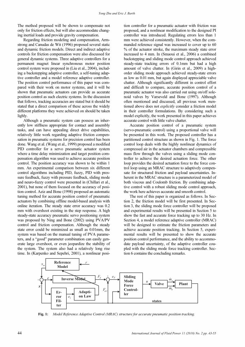
partitioned control structure as shown in Fig. 1. The force
control loop deals with the highly nonlinear dynamics of
compressed air in the actuator chambers and compressible
mass flow through the valves using a sliding mode con-
troller to achieve the desired actuation force. The other
loop provides the desired actuation force to the force con-
trol loop using an MRAC structure to adaptively compen-
sate for structured friction and payload uncertainties. In-
herent in the MRAC structure is a parameterized model of
both viscous and Coulomb friction. By combining adap-
tive control with a robust sliding mode control approach,
the work here achieves accurate and smooth control.
The rest of this paper is organized as follows. In Sec-
tion 2, the friction model will be first presented. In Sec-
tion 3, the sliding mode force controller will be proposed
and experimental results will be presented in Section 5 to
show the fast and accurate force tracking up to 30 Hz. In
Section 4, a model reference adaptive controller (MRAC)
will be designed to estimate the friction parameters and
achieve accurate position tracking. In Section 5, experi-
mental results will be presented to show the accurate
position control performance, and the ability to accommo-
date payload uncertainty, of the adaptive controller cou-
pled with the sliding mode force tracking controller. Sec-
tion 6 contains the concluding remarks.
Fig. 1: Model Reference Adaptive Control (MRAC) structure for accurate pneumatic position tracking.
Accurate sub-Millimeter Servo-Pneumatic Tracking using Model Reference Adaptive Control (MRAC)
International Journal of Fluid Power 11 (2010) No. 2 pp. 43-54 45
2 Friction Model
In order to offer model-based friction compensation
and achieve accurate position control, a reasonably
accurate and implementable friction model needs to be
chosen first. Although friction occurs in almost all
mechanical systems, there is no universal friction
model applicable to all systems given that the mecha-
nisms of friction are a collection of a number of more
fundamental surface interaction and fluid related physi-
cal phenomena. For different systems and control ob-
jectives, different friction models are adopted to em-
phasize the regimes and mechanisms of friction most
dominant or having the most impact on the chosen
objective. A simple Gaussian exponential static friction
model, represented in Eq. 1, is often chosen. This de-
scription of friction is a function of instantaneous slid-
ing velocity v(t) and captures three friction phenomena:
Coulomb, viscous and Stribeck friction.
2
s
c
[ ( ) / ]
s v
[ ( )] sgn[ ( )]
sgn( ( )) ( )v t v
F v t F v t
F e v t F v t−
= +
+
(1)
where Fc is the Coulomb friction, Fs is the magnitude
of Stribeck friction, vs is the characteristic velocity of
Stribeck friction, and Fv is the linear viscous friction
coefficient. By choosing different parameters, different
friction models can be realized. This is an adequate
model for describing the zero velocity friction force.
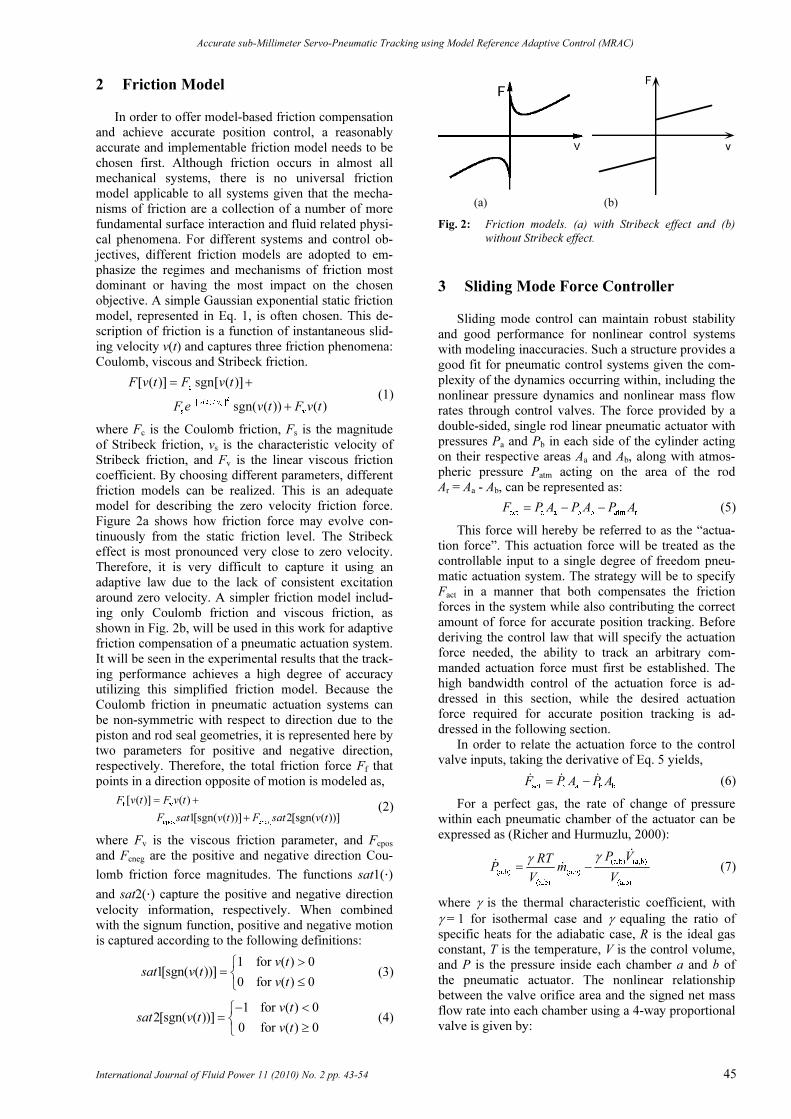
Figure 2a shows how friction force may evolve con-
tinuously from the static friction level. The Stribeck
effect is most pronounced very close to zero velocity.
Therefore, it is very difficult to capture it using an
adaptive law due to the lack of consistent excitation
around zero velocity. A simpler friction model includ-
ing only Coulomb friction and viscous friction, as
shown in Fig. 2b, will be used in this work for adaptive
friction compensation of a pneumatic actuation system.
It will be seen in the experimental results that the track-
ing performance achieves a high degree of accuracy
utilizing this simplified friction model. Because the
Coulomb friction in pneumatic actuation systems can
be non-symmetric with respect to direction due to the
piston and rod seal geometries, it is represented here by
two parameters for positive and negative direction,
respectively. Therefore, the total friction force Ff that
points in a direction opposite of motion is modeled as,
f v
cpos cneg
[ ( )] ( )
1[sgn( ( ))] 2[sgn( ( ))]
F v t F v t
F sat v t F sat v t
= +
+
(2)
where Fv is the viscous friction parameter, and Fcpos
and Fcneg are the positive and negative direction Cou-
lomb friction force magnitudes. The functions sat1(⋅)
and sat2(⋅) capture the positive and negative direction
velocity information, respectively. When combined
with the signum function, positive and negative motion
is captured according to the following definitions:
1 for ( ) 0
1[sgn( ( ))]0 for ( ) 0
v t
sat v t
v t
>⎧= ⎨
≤⎩ (3)
1 for ( ) 0
2[sgn( ( ))]0 for ( ) 0
v t
sat v t
v t
− <⎧= ⎨
≥⎩ (4)
v
F
(a) (b)
Fig. 2: Friction models. (a) with Stribeck effect and (b)
without Stribeck effect.
3 Sliding Mode Force Controller
Sliding mode control can maintain robust stability
and good performance for nonlinear control systems
with modeling inaccuracies. Such a structure provides a
good fit for pneumatic control systems given the com-
plexity of the dynamics occurring within, including the
nonlinear pressure dynamics and nonlinear mass flow
rates through control valves. The force provided by a
double-sided, single rod linear pneumatic actuator with
pressures Pa and Pb in each side of the cylinder acting
on their respective areas Aa and Ab, along with atmos-
pheric pressure Patm acting on the area of the rod
Ar = Aa - Ab, can be represented as:
act a a b b atm r
F P A P A P A= − − (5)
This force will hereby be referred to as the “actua-
tion force”. This actuation force will be treated as the
controllable input to a single degree of freedom pneu-
matic actuation system. The strategy will be to specify
Fact in a manner that both compensates the friction
forces in the system while also contributing the correct
amount of force for accurate position tracking. Before
deriving the control law that will specify the actuation
force needed, the ability to track an arbitrary com-
manded actuation force must first be established. The
high bandwidth control of the actuation force is ad-
dressed in this section, while the desired actuation
force required for accurate position tracking is ad-
dressed in the following section.
In order to relate the actuation force to the control
valve inputs, taking the derivative of Eq. 5 yields,
act a a b b
F P A P A= −� � � (6)
For a perfect gas, the rate of change of pressure
within each pneumatic chamber of the actuator can be
expressed as (Richer and Hurmuzlu, 2000):
(a,b) (a,b)
(a,b) (a,b)
(a,b) (a,b)
P VRTP m
V V
γγ= −
�
�
� (7)
where γ is the thermal characteristic coefficient, with
γ = 1 for isothermal case and γ equaling the ratio of
specific heats for the adiabatic case, R is the ideal gas
constant, T is the temperature, V is the control volume,
and P is the pressure inside each chamber a and b of
the pneumatic actuator. The nonlinear relationship
between the valve orifice area and the signed net mass
flow rate into each chamber using a 4-way proportional
valve is given by:
Yong Zhu and Eric J. Barth
46 International Journal of Fluid Power 11 (2010) No. 2 pp. 43-55
a v a u d
( , )m A P P= Ψ� (8)
b v b u d
( , )m A P P= − Ψ� (9)
where Av is the high-bandwidth controlled orifice area
of the valve and Ψ(Pu, Pd) is the area normalized mass
flow rate relationship as a function of the pressure
upstream and downstream across each flow channel of
the valve. By virtue of the physical arrangement of the
valve, the driving pressures of Ψ(Pu, Pd), and ulti-
mately the sign of the mass flow rate, are dependent on
the sign of the valve’s orifice “area”. The convention
used here will be that a positive area Av indicates that
the spool of the proportional valve is positioned such
that a flow orifice of area Av connects the high pressure
pneumatic supply to one side of the pneumatic cylin-
der, and thereby promotes a positive mass flow rate
into the cylinder chamber. A negative area Av indicates
that the spool of the proportional valve is positioned
such that an orifice of area Av connects one side of the
pneumatic cylinder to atmospheric pressure, and
thereby promotes a negative mass flow rate (exhaust
from the cylinder chamber). The areas of the two flow
paths to ports a and b are then equal and opposite by
virtue of the four-way valve design. Using this conven-
tion, the area normalized mass flow rate can be written
as:
s
u d
atm
( , ) for 0( , )
( , ) for 0
P P AP P
P P A
Ψ ≥⎧Ψ = ⎨
Ψ <⎩ (10)
A common mass flow rate model used for com-
pressible gas flowing through a valve is given by
(Richer and Hurmuzlu, 2000),
u d
1 f u dr
u
1/ ( 1) /
2 f u d d
u u
( , )
if (choked)
1 otherwise (unchoked)
k k k
P P
C C P PC
PT
C C P P P
P PT
−
Ψ =
⎧≤⎪
⎪⎨
⎛ ⎞ ⎛ ⎞⎪−⎜ ⎟ ⎜ ⎟⎪
⎝ ⎠ ⎝ ⎠⎩
(11)
where Pu and Pd are the upstream and downstream
pressures, Cf is the discharge coefficient of the valve, k
is the ratio of specific heats, Cr is the pressure ratio that
divides the flow regimes into choked and unchoked
flow and C1 and C2 are constants defined as:
( 1) /( 1)
1
2
1
k kk
CR k
+ −
⎛ ⎞= ⎜ ⎟
+⎝ ⎠ and
)1(
22
−
=
kR
kC (12)
The objective of the actuation force controller is to
make the actuation force Fact track a desired force tra-
jectory Fd (to be specified later). The actuation force
tracking error is defined as eF = Fact Fd. It can be seen
from Eq. 6 to 9 that act
F� is directly related to the con-
trol input u = Av through the pressure dynamics. There-
fore, the dynamic model of the pneumatic actuator
force control is a first order nonlinear system if the
dynamics of the valve spool position control is ne-
glected (i.e. the bandwidth of the spool valve position
control is much higher than the desired force control
bandwidth). By combining Eq. 6 to 12, this single input
dynamic system can be put into standard functional
form as:
act a,b a,b a,b a,b a,b
( , , ) ( , )F f P V V b P V u= +� � (13)
where u = Av. The standard time varying sliding surface
used in sliding mode control theory (Slotine and Li,
1991) is defined as edt
ds
n 1−
⎟⎠
⎞⎜⎝
⎛+= λ . For a first order
system where n = 1, s simply becomes:
F act d a a b b atm r d
s e F F P A P A P A F= = − = − − − (14)
Taking the time derivative of s and substituting
Eq. 7 into s� yields the sliding mode equation:
a a b b
a a b b d
a a b b
PV PVRT RTs m A m A F
V V V V
⎛ ⎞ ⎛ ⎞= − − − −⎜ ⎟ ⎜ ⎟⎝ ⎠ ⎝ ⎠
� �
�
� � �
(15)
Equating Eq. 14 to zero and substituting Eq. 8 and 9
into Eq. 14 to solve for the equivalent control law
gives:
2 2
a a b b b a a b d
eq
a b a u d b a b u d
( )
[ ( , ) ( , )]
P A V P A V x V V Fu
RT AV P P AV P P
+ +=
Ψ + Ψ
�
�
(16)
where a a b b
x V A V A= = −� �
� relating the actuator’s
chamber volumes to the rod position x.
A discontinuous robustness term is then added
across the sliding surface to achieve the typical sliding
mode control law:
F
eq eq
esu u sat u satκ κ
ϕ ϕ
⎛ ⎞ ⎛ ⎞= − = −⎜ ⎟ ⎜ ⎟
⎝ ⎠ ⎝ ⎠ (17)
where κ and φ are positive constants that specify the
boundary layer (Slotine and Li, 1991). This control law
can be easily proven to be Lyapunov stable.
4 Design of a MRAC for Adaptive Fric-
tion Compensation
A model reference adaptive controller is designed
for friction compensation in this section. The friction
parameters Fv, Fcpos and Fcneg will be estimated by the
adaption law and then utilized to derive the appropriate
desired actuation force Fd to make the actuator rod
position x track a desired trajectory. The choice of a set
of model parameters to be estimated adaptively must be
uniquely determinable from the model. The open loop
dynamics of the pneumatic cylinder are represented
according to the following model:
act
v cpos cneg
cos
1[sgn( )] 2[sgn( )]
F Mx Mg
F x F sat x F sat x
θ= − +
+ +
��
� � �
(18)
where θ represents the actuator’s angular deviation from
a vertical orientation. Although it would appear at first
that the mass M should be included in the set of parame-
ters to be estimated, it will be shown that it appears as a
common factor that simply scale the friction parameters.
Also not obvious from looking at the model of Eq. 18
is the fact that a constant force offset from gravity, if the
piston is oriented with a component aligned with gravity,
is able to be encoded using the asymmetric Coulomb
friction parameters Fcpos and Fcneg. The inherent estimation
of the inertia and gravity offset will be demonstrated.
An important lesson that was learned from initially
choosing only one Coulomb friction parameter, represent-
ing a symmetric Coulomb friction model, was that the
Accurate sub-Millimeter Servo-Pneumatic Tracking Using Model Reference Adaptive Control (MRAC)
International Journal of Fluid Power 11 (2010) No. 2 pp. 43-55 47
adaptive controller will not able to successfully minimize
the position tracking error. The Coulomb friction of a
typical double-acting, single-rod, pneumatic actuator is
asymmetric. Therefore, if the position errors in the posi-
tive and negative directions are mixed together as the error
information used to adaptively estimate one Coulomb
friction parameter, this parameter will not converge but
simply “roams” between an upper and lower bound.
In pursuing a model reference adaptive approach, the
following reference model was utilized to generate the
ideal, or model, dynamic position response xm(t) to the
commanded position signal r(t):
2 2
m n m n m n2x x x rξω ω ω+ + =�� � (19)
The desired model-based actuation force, that sub-
sequently becomes the command that is feed into the
sliding mode force controller, is chosen as,
d m v p
v cpos cneg
( ) cos
ˆ ˆ ˆ1[sgn( )] 2[sgn( )]
F M x k e k e Mg
F x F sat x F sat x
θ= + + − +
+ +
�� �
� � �
(20)
where the position error is given by e = xm x. Control
gains kv and kp are positive constants chosen to reflect the
desired performance specifications in tracking the refer-
ence model. Friction parameter estimates are given by
v
ˆF , cpos
ˆF and cneg
ˆF . Combining Eq. 18 and 20 gives:
v cpos cneg
m v p v
cpos cneg
1[sgn( )] 2[sgn( )]
ˆ( )
ˆ ˆ1[sgn( )] 2[sgn( )]
Mx F x F sat x F sat x
M x k e k e F x
F sat x F sat x
+ + + =
+ + + +
+
�� � � �
�� � �
� �
(21)
subtracting xM �� from both sides of Eq. 21 yields:
v cpos cneg
m v p v
cpos cneg
1[sgn( )] 2[sgn( )]
ˆ[( ) ]
ˆ ˆ1[sgn( )] 2[sgn( )]
F x F sat x F sat x
M x x k e k e F x
F sat x F sat x
+ + =
− + + + +
+
� � �
�� �� � �
� �
(22)
since exxm
������ =− , Eq. 22 can be rearranged as:
v p
1
v v cpos cpos
cneg cneg
ˆ ˆ[( ) ( ) 1[sgn( )]
ˆ( ) 2[sgn( )]]
e k e k e
M F F x F F sat x
F F sat x
−
+ + =
− + −
+ −
�� �
� �
�
(23)
Note that M appears as a common factor of the fric-
tion parameters in Eq. 23. This fact enables the adaptive
estimation of the friction parameters to also include an
inherent estimation of the actuator’s inertia given that it
represents a constant scaling of the friction parameters.
Equation 23 can be rewritten in matrix form as:
]
v p
v v
1
cpos cpos
cneg cneg
ˆ
ˆ1[sgn( )] 2[sgn( )]
ˆH
a
e k e k e
F F
M x sat x sat x F F
F F
−
+ + =
⎡ ⎤−⎢ ⎥
⎡ −⎢ ⎥⎣⎢ ⎥
−⎢ ⎥⎣ ⎦�
�� �
� � ����������������
�������
(24)
Defining H and a~ as above, Eq. 24 can be written
more compactly as:
1
v pe k e k e M Ha−
+ + =�� � � (25)
Equation 25 can be represented in the Laplace do-
main as (note that this s is not the same as the sliding
surface s):
1
2
v p
1( )e s M Ha
s k s k
−
=
+ +
� (26)
A filtered error signal is defined as:
e1(s) = (s + η)e(s) (expressed in Laplace domain),
where η is a positive constant. The role of e1 will be to
preserve the strictly positive real property of the trans-
fer function relating the estimated signal aHM~1−
to
the error signal used for the adaption. Substituting
Eq. 26 into e1(s) gives this filtered error signal:
1
1 2
v p
( )s
e s M Has k s k
η−
+
=
+ +
� (27)
Equation 27 forms the basis of the adaptive control-
ler. Eq. 27 can be rewritten in state space form (with 1e
as the output):
aHBMAXX~1−
+=�
(28)
CXe =
1 (29)
where e
Xe
⎡ ⎤= ⎢ ⎥⎣ ⎦�
, p v
0 1A
k k
⎡ ⎤= ⎢ ⎥− −⎣ ⎦
, 0
1B
⎡ ⎤= ⎢ ⎥⎣ ⎦
and
C = [η 1].
Based on the Kalman-Yakubovich lemma (Slotine
and Li, 1991), since the transfer function h(s) = C[sI -
A]-1B = (s + η)/(s2 + kvs + kp) > 0 is strictly positive
real for an appropriate choice of η, kv and kp, there exist
two symmetric positive definite constant matrices P
and Q for the system shown in Eq. 28 and 29, such that
ATP + PA = -Q and PB = CT. A Lyapunov function
candidate can be chosen as the following equation
according to a standard form to stabilize the system:
1( , )
T TV X a X PX a a
−
= + Γ� � � (30)
where Γ = diag(γ1, γ2, γ3), γi ≥ 0 (i = 1,2,3, ), which is
also a symmetric positive definite constant matrix.
Taking the time derivative of V gives:
1 1( , ) T T T T
V X a X PX X PX a a a a− −
= + + à + � �� � �
� � � � � (31)
Since both XPXT
� and aaT
�~~ 1−
Γ are 11× matrices,
XPXPXXTT
��
= and aaaaTT
��~~~~ 11 −−
Γ=Γ , Eq. 29 can be
simplified as:
1( , ) 2 2T TV X a X PX a a
−
= + à �� �
� � � (32)
Substituting Eq. 28 into Eq. 32, along with the fact
that PA is symmetric, ATP = PA, and BT
P = C, gives,
)~(~2)~,( 1
1
1aeMHaQXXaXV
TTT�
�
−−
Γ++−= (33)
If we choose 1
1~
eMHaT −
Γ−=� to eliminate the sec-
ond term, then 0)~,( ≤−= QXXaXVT
� and ensures
stability since Q is positive definite by the Kalman-
Yakubovich lemma. Further, since
Yong Zhu and Eric J. Barth
48 International Journal of Fluid Power 11 (2010) No. 2 pp. 43-55
v v vv
cpos cpos cpos cpos
cnegcneg cneg cneg
ˆ
ˆ ˆ
ˆ ˆ
ˆ
ˆ ˆ
pp
F F FF
a F F F F p p
FF F F
⎡ ⎤ ⎡ ⎤− ⎡ ⎤⎢ ⎥ ⎢ ⎥⎢ ⎥
= − = − = −⎢ ⎥ ⎢ ⎥⎢ ⎥⎢ ⎥ ⎢ ⎥⎢ ⎥
−⎢ ⎥ ⎢ ⎥⎣ ⎦⎣ ⎦ ⎣ ⎦
�
��� ���
(34)
taking the time derivative of Eq. 34 yields pa��
ˆ~
−= .
The following adaption law results:
1
1
1
1 2 3 1
ˆ
( , , ) 1[sgn( )]
2[sgn( )]
Tp H M e
x
diag sat x M e
sat x
γ γ γ
−
−
= Γ
⎡ ⎤⎢ ⎥= ⎢ ⎥⎢ ⎥⎣ ⎦
�
�
�
�
(35)
Equation 35 can be simplified as:
v1
1
cpos 2 1
3cneg
ˆ
ˆ 1[sgn( )]
2[sgn( )]ˆ
Fx
F sat x M e
sat xF
γ
γ
γ
−
⎡ ⎤⎡ ⎤⎢ ⎥⎢ ⎥⎢ ⎥ = ⎢ ⎥⎢ ⎥⎢ ⎥⎢ ⎥ ⎣ ⎦
⎢ ⎥⎣ ⎦
�
�
�
�
��
(36)
Equation 36 is the update law for the estimation of
the friction parameters. The standard derivation is
based on Lyapunov stability theory.
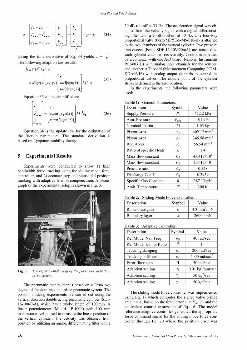
5 Experimental Results
Experiments were conducted to show 1) high
bandwidth force tracking using the sliding mode force
controller, and 2) accurate step and sinusoidal position
tracking with adaptive friction compensation. A photo-
graph of the experimental setup is shown in Fig. 3.
Fig. 3: The experimental setup of the pneumatic actuation
servo system.
The pneumatic manipulator is based on a Festo two
degree-of-freedom pick and place pneumatic system. The
position tracking experiments are carried out using the
vertical direction double acting pneumatic cylinder (SLT-
16-100-P-A), which has a stroke length of 100 mm. A
linear potentiometer (Midori LP-100F) with 100 mm
maximum travel is used to measure the linear position of
the vertical cylinder. The velocity was obtained from
position by utilizing an analog differentiating filter with a
20 dB roll-off at 33 Hz. The acceleration signal was ob-
tained from the velocity signal with a digital differentiat-
ing filter with a 20 dB roll-off at 30 Hz. One four-way
proportional valve (Festo MPYE-5-M5-010-B) is attached
to the two chambers of the vertical cylinder. Two pressure
transducers (Festo SDE-16-10V/20mA) are attached to
each cylinder chamber, respectively. Control is provided
by a computer with one A/D board (National Instruments
PCI-6031E) with analog input channels for the sensors,
and another A/D board (Measurement Computing PCIM-
DDA06/16) with analog output channels to control the
proportional valves. The middle point of the cylinder
stroke is defined as the zero position.
In the experiments, the following parameters were
used:
Table 1: General Parameters:
Description Symbol Value
Supply Pressure Ps
652.2 kPa
Atm. Pressure Patm
101 kPa
Nominal Inertia M 1.05 kg
Piston Area Aa
402.12 mm2
Piston Area Ab
345.58 mm2
Rod Areas Ar
56.54 mm2
Ratio of specific Heats k 1.4
Mass flow constant C1
4.0418×10⁵
Mass flow constant C2
1.5617×10⁴
Pressure ratio Cr
0.528
Discharge Coeff Cf
0.2939
Specific Gas Constant R 287 J/kg/K
Amb. Temperature T 300 K
Table 2: Sliding Mode Force Controller:
Description Symbol Value
Robustness gain κ 4.3 mm2/mN
Boundary layer φ 26000 mN
Table 3: Adaptive Controller:
Description Symbol Value
Ref Model Nat. Freq ωn
40 rad/sec
Ref Model Damp. Ratio ξ 1
Tracking damping kv
200 rad/sec
Tracking stiffness kp
4000 rad/sec2
Error filter zero η 30 rad/sec
Adaption scaling 1γ 0.01 kg2/mm/sec
Adaption scaling 2γ 50 kg2/sec
Adaption scaling 3γ 50 kg2/sec
The sliding mode force controller was implemented
using Eq. 17 which computes the signed valve orifice
area u = Av based on the force error eF = Fact Fd and the
equivalent control expression of Eq. 16. The model
reference adaptive controller generated the appropriate
force command signal for the sliding mode force con-
troller through Eq. 20 where the position error was

Accurate sub-Millimeter Servo-Pneumatic Tracking Using Model Reference Adaptive Control (MRAC)
International Journal of Fluid Power 11 (2010) No. 2 pp. 43-55 49
computed as e = xm x with the model position response
xm(t) computed from Eq. 19 based on the commanded
position r. The adaptive friction parameters of Eq. 20
were updated using Eq. 36 which utilizes the filtered
error signal computed as e1(s) = (s + η)e(s).
5.1 Sliding Mode Force Controller Performance
The actuation force tracking performance of the
sliding mode force controller for 1 Hz and 20 Hz sinu-
soidal inputs is shown in Fig. 4. Up to 30 Hz
(188 rad/sec), the valve and controller can still provide
good force tracking. In these experiments, the cylinder
rod is fixed at the middle stroke position.
0 0.2 0.4 0.6 0.8 1 1.2 1.4 1.6 1.8 2-20
0
20
40
60
80
100
120
140
Time (sec)
Fo
rce
(N
)
Actuation force tracking
desired output force
actual output force
(a) 1 Hz actuation force tracking
0 0.05 0.1 0.15 0.2 0.25 0.3-20
40
60
80
100
120
140
Time (sec)
Forc
e (N
)
Actuation force tracking
desired output force
actual output force
0
20
(b) 20 Hz actuation force tracking
Fig. 4: Experimental results of the sliding mode controller
actuator force tracking for sinusoidal input with
frequency: (a) 1 Hz and (b) 20 Hz.
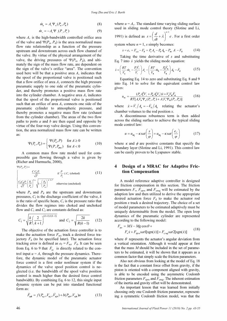
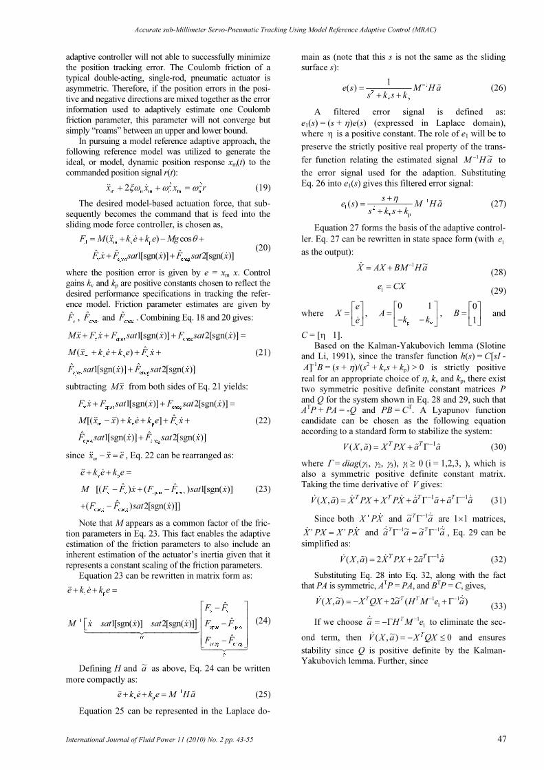
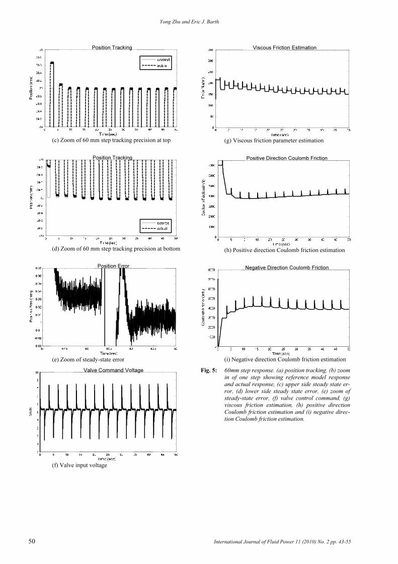
5.2 MRAC Controller Performance
Step tracking of 60 mm amplitude is presented in
Fig. 5. The moving mass of the vertical cylinder was
0.67 kg and a 0.38 kg mass was attached to it as a pay-
load. It can be seen that the adaptive friction compensa-
tion can effectively compensate the unmodeled changes in
friction behavior induced by the change in amplitude. The
parameters all converge quickly. The steady state error of
the step response is within 0.05 mm. A close inspection of
the steady-state error reveals that the accuracy is as good
as perhaps 0.035 mm; a spectral analysis of the error
signal reveals distinct peaks at 60 Hz and 180 Hz suggest-
ing noise from electrical power and not actual displace-
ment in steady-state. The rise time (10 % to 90 %) is
about 200 ms for step inputs from -30 mm to 30 mm. The
valve command shows little chatter. It is conjectured that
the combined feed forward aspects offered by the parame-
ters estimated by the adaptive portion of the controller,
combined with a boundary-layer sliding mode controller,
allows for smooth control inputs to the plant.
Sinusoidal tracking of 0.5 Hz and 1 Hz with a 60 mm
amplitude are presented in Fig. 6 and 7. It can be seen that
the adaptive friction compensation can effectively com-
pensate for unmodeled changes in friction behavior at
different velocities. For the 0.5 Hz sinusoidal input, the
tracking error is within 0.7 mm. For the 1 Hz sinusoidal
input, the tracking error is within 1.2 mm.
In all tracking cases, the higher bandwidth of the slid-
ing mode force tracking controller (greater than
188 rad/sec) relative to the parameter adaption (at
30 rad/sec), along with the fact that sliding mode control
offers a robust control approach, ensures stable interaction
between the force tracking dynamics and the adaptive
controller.
5.2.1 60mm Step Tracking
0 5 10 15 20 25 30 35 40 45 50-50
-40
-30
-20
-10
0
10
20
30
40
Time (sec)
Position (mm)
Position Tracking
desired
actual
(a) 60 mm step tracking
21 21.5 22 22.5 23 23.5 24 24.5 25-40
-30
-20
-10
0
10
20
30
40
Time (sec)
Position (mm)
Position Tracking
desired
actual
(b) Zoom in time showing the shape of the reference
model response to a step input and the MRAC controller’s
performance in tracking it
Yong Zhu and Eric J. Barth
50 International Journal of Fluid Power 11 (2010) No. 2 pp. 43-55
0 5 10 15 20 25 30 35 40 45 5029
29.2
29.4
29.6
29.8
30
30.2
30.4
30.6
30.8
31
Time (sec)
Position (mm)
Position Tracking
desired
actual
(c) Zoom of 60 mm step tracking precision at top
0 5 10 15 20 25 30 35 40 45 50-31
-30.8
-30.6
-30.4
-30.2
-30
-29.8
-29.6
-29.4
-29.2
-29
Time (sec)
Position (mm)
Position Tracking
desired
actual
(d) Zoom of 60 mm step tracking precision at bottom
47 47.5 48 48.5 49 49.5 50-0.03
-0.02
-0.01
0
0.01
0.02
0.03
0.04
0.05
0.06
0.07Position Error
Time (sec)
Position Error(mm)
(e) Zoom of steady-state error
0 5 10 15 20 25 30 35 40 45 500
1
2
3
4
5
6
7
8
9
10Valve Command Voltage
Time (sec)
Volts
(f) Valve input voltage
0 5 10 15 20 25 30 35 40 45 500
50
100
150
200
250
300
350
Time (sec)
Fv (mN.s/m)
Viscous Friction Estimation
(g) Viscous friction parameter estimation
0 5 10 15 20 25 30 35 40 45 500
1000
2000
3000
4000
5000
6000
7000
Time (sec)
Coulomb Friction(mN)
Positive Direction Coulomb Friction
(h) Positive direction Coulomb friction estimation
0 5 10 15 20 25 30 35 40 45 500
1000
2000
3000
4000
5000
6000
7000
8000
Time (sec)
Coulomb Friction(mN)
Negative Direction Coulomb Friction
(i) Negative direction Coulomb friction estimation
Fig. 5: 60mm step response. (a) position tracking, (b) zoom
in of one step showing reference model response
and actual response, (c) upper side steady state er-
ror, (d) lower side steady state error, (e) zoom of
steady-state error, (f) valve control command, (g)
viscous friction estimation, (h) positive direction
Coulomb friction estimation and (i) negative direc-
tion Coulomb friction estimation.
Accurate sub-Millimeter Servo-Pneumatic Tracking Using Model Reference Adaptive Control (MRAC)
International Journal of Fluid Power 11 (2010) No. 2 pp. 43-55 51
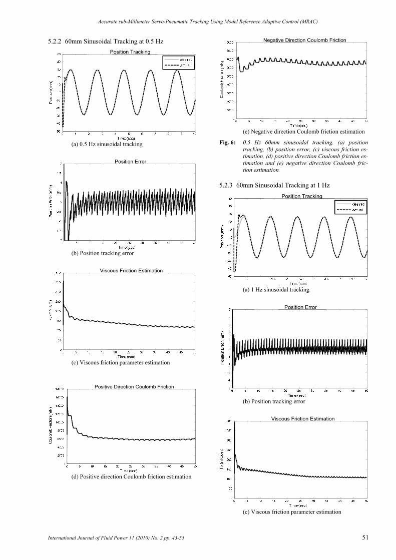
5.2.2 60mm Sinusoidal Tracking at 0.5 Hz
0 1 2 3 4 5 6 7 8 9 10-50
-40
-30
-20
-10
0
10
20
30
40
50
Time (sec)
Position (mm)
Position Tracking
desired
actual
(a) 0.5 Hz sinusoidal tracking
0 5 10 15 20 25 30 35 40 45 50-2
-1.5
-1
-0.5
0
0.5
1
1.5
2
Time (sec)
Position Error (mm)
Position Error
(b) Position tracking error
0 5 10 15 20 25 30 35 40 45 500
50
100
150
200
250
300
350
400
Time (sec)
Fv (mN.s/m)
Viscous Friction Estimation
(c) Viscous friction parameter estimation
0 5 10 15 20 25 30 35 40 45 500
2000
4000
6000
8000
10000
12000
14000
16000
18000
Time (sec)
Coulomb Friction (mN)
Positive Direction Coulomb Friction
(d) Positive direction Coulomb friction estimation
0 5 10 15 20 25 30 35 40 45 500
1000
2000
3000
4000
5000
6000
7000
8000
9000
Time (sec)
Coulomb Friction (mN)
Negative Direction Coulomb Friction
(e) Negative direction Coulomb friction estimation
Fig. 6: 0.5 Hz 60mm sinusoidal tracking. (a) position
tracking, (b) position error, (c) viscous friction es-
timation, (d) positive direction Coulomb friction es-
timation and (e) negative direction Coulomb fric-
tion estimation.
5.2.3 60mm Sinusoidal Tracking at 1 Hz
0 0.5 1 1.5 2 2.5 3 3.5 4 4.5 5-50
-40
-30
-20
-10
0
10
20
30
40
50
Time (sec)
Position (mm)
Position Tracking
desired
actual
(a) 1 Hz sinusoidal tracking
0 5 10 15 20 25 30 35 40 45 50-5
-4
-3
-2
-1
0
1
2
3
4
5
Time (sec)
Position Error (mm)
Position Error
(b) Position tracking error
0 5 10 15 20 25 30 35 40 45 500
50
100
150
200
250
300
350
400
Time (sec)
Fv (mN.s/m)
Viscous Friction Estimation
(c) Viscous friction parameter estimation
Yong Zhu and Eric J. Barth
52 International Journal of Fluid Power 11 (2010) No. 2 pp. 43-55
0 5 10 15 20 25 30 35 40 45 500
2000
4000
6000
8000
10000
12000
14000
16000
18000
Time (sec)
Coulomb Friction(mN)
Positive Direction Coulomb Friction
(d) Positive direction Coulomb friction estimation
0 5 10 15 20 25 30 35 40 45 500
2000
4000
6000
8000
10000
12000
Time (sec)
Coulomb Friction (mN)
Negative Direction Coulomb Friction
(e) Negative direction Coulomb friction estimation
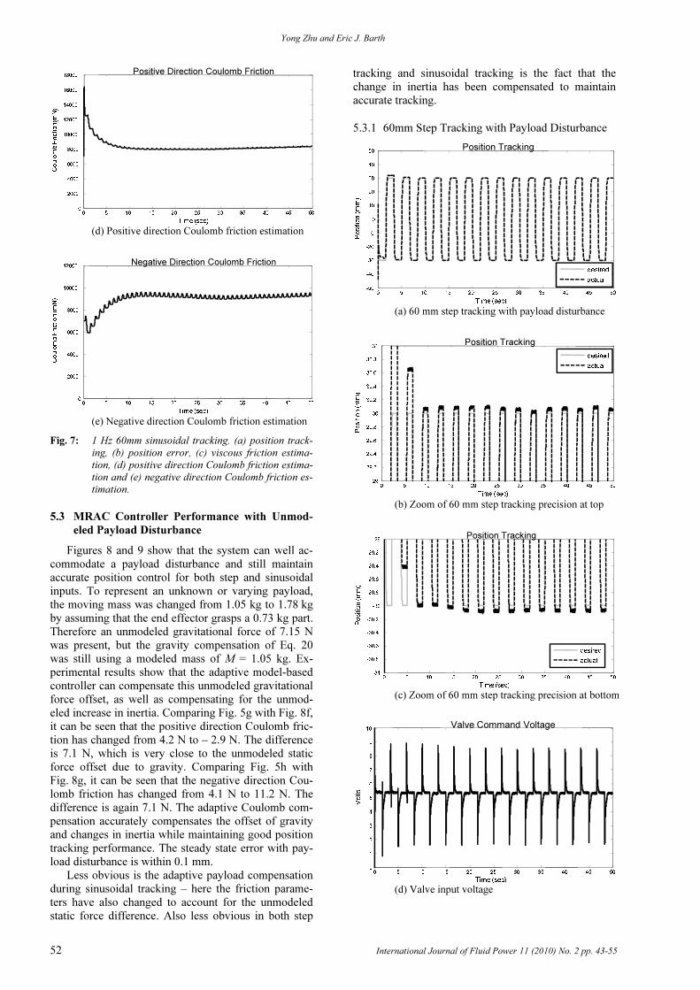
Fig. 7: 1 Hz 60mm sinusoidal tracking. (a) position track-
ing, (b) position error, (c) viscous friction estima-
tion, (d) positive direction Coulomb friction estima-
tion and (e) negative direction Coulomb friction es-
timation.
5.3 MRAC Controller Performance with Unmod-
eled Payload Disturbance
Figures 8 and 9 show that the system can well ac-
commodate a payload disturbance and still maintain
accurate position control for both step and sinusoidal
inputs. To represent an unknown or varying payload,
the moving mass was changed from 1.05 kg to 1.78 kg
by assuming that the end effector grasps a 0.73 kg part.
Therefore an unmodeled gravitational force of 7.15 N
was present, but the gravity compensation of Eq. 20
was still using a modeled mass of M = 1.05 kg. Ex-
perimental results show that the adaptive model-based
controller can compensate this unmodeled gravitational
force offset, as well as compensating for the unmod-
eled increase in inertia. Comparing Fig. 5g with Fig. 8f,
it can be seen that the positive direction Coulomb fric-
tion has changed from 4.2 N to – 2.9 N. The difference
is 7.1 N, which is very close to the unmodeled static
force offset due to gravity. Comparing Fig. 5h with
Fig. 8g, it can be seen that the negative direction Cou-
lomb friction has changed from 4.1 N to 11.2 N. The
difference is again 7.1 N. The adaptive Coulomb com-
pensation accurately compensates the offset of gravity
and changes in inertia while maintaining good position
tracking performance. The steady state error with pay-
load disturbance is within 0.1 mm.
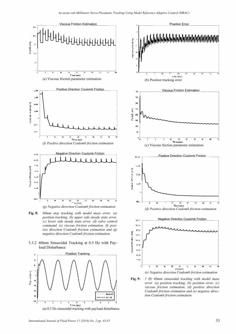
Less obvious is the adaptive payload compensation
during sinusoidal tracking – here the friction parame-
ters have also changed to account for the unmodeled
static force difference. Also less obvious in both step
tracking and sinusoidal tracking is the fact that the
change in inertia has been compensated to maintain
accurate tracking.
5.3.1 60mm Step Tracking with Payload Disturbance
0 5 10 15 20 25 30 35 40 45 50-50
-40
-30
-20
-10
0
10
20
30
40
50
Time (sec)
Position (mm)
Position Tracking
desired
actual
(a) 60 mm step tracking with payload disturbance
0 5 10 15 20 25 30 35 40 45 5029
29.2
29.4
29.6
29.8
30
30.2
30.4
30.6
30.8
31
Time (sec)
Position (mm)
Position Tracking
desired
actual
(b) Zoom of 60 mm step tracking precision at top
0 5 10 15 20 25 30 35 40 45 50-31
-30.8
-30.6
-30.4
-30.2
-30
-29.8
-29.6
-29.4
-29.2
-29
Time (sec)
Position (mm)
Position Tracking
desired
actual
(c) Zoom of 60 mm step tracking precision at bottom
0 5 10 15 20 25 30 35 40 45 500
1
2
3
4
5
6
7
8
9
10Valve Command Voltage
Time (sec)
Volts
(d) Valve input voltage
Accurate sub-Millimeter Servo-Pneumatic Tracking Using Model Reference Adaptive Control (MRAC)
International Journal of Fluid Power 11 (2010) No. 2 pp. 43-55 53
0 5 10 15 20 25 30 35 40 45 500
50
100
150
200
250
Time (sec)
Fv (mN.s/m)
Viscous Friction Estimation
(e) Viscous friction parameter estimation
0 5 10 15 20 25 30 35 40 45 50
-4000
-2000
0
2000
4000
6000
8000
Time (sec)
Coulomb Friction(mN)
Positive Direction Coulomb Friction
(f) Positive direction Coulomb friction estimation
0 5 10 15 20 25 30 35 40 45 50-2000
0
2000
4000
6000
8000
10000
12000
14000
Time (sec)
Coulomb Friction(mN)
Negative Direction Coulomb Friction
(g) Negative direction Coulomb friction estimation
Fig. 8: 60mm step tracking with model mass error. (a)
position tracking, (b) upper side steady state error,
(c) lower side steady state error, (d) valve control
command, (e) viscous friction estimation, (f) posi-
tive direction Coulomb friction estimation and (g)
negative direction Coulomb friction estimation.
5.3.2 60mm Sinusoidal Tracking at 0.5 Hz with Pay-
load Disturbance
0 1 2 3 4 5 6 7 8 9 10-50
-40
-30
-20
-10
0
10
20
30
40
Time (sec)
Position (mm)
Position Tracking
desired
actual
(a) 0.5 Hz sinusoidal tracking with payload disturbance
0 5 10 15 20 25 30 35 40 45 50-5
-4
-3
-2
-1
0
1
2
Time (sec)
Position Error (mm)
Position Error
(b) Position tracking error
0 5 10 15 20 25 30 35 40 45 500
50
100
150
200
250
300
350
400
Time (sec)
Fv (mN.s/m)
Viscous Friction Estimation
(c) Viscous friction parameter estimation
0 5 10 15 20 25 30 35 40 45 50-5000
0
5000
10000
15000
20000
Time (sec)
Coulomb Friction (mN)
Positive Direction Coulomb Friction
(d) Positive direction Coulomb friction estimation
0 5 10 15 20 25 30 35 40 45 500
2000
4000
6000
8000
10000
12000
14000
16000
18000
Time (sec)
Coulomb Friction (mN)
Negative Direction Coulomb Friction
(e) Negative direction Coulomb friction estimation
Fig. 9: 1 Hz 60mm sinusoidal tracking with model mass
error. (a) position tracking, (b) position error, (c)
viscous friction estimation, (d) positive direction
Coulomb friction estimation and (e) negative direc-
tion Coulomb friction estimation.
Yong Zhu and Eric J. Barth
54 International Journal of Fluid Power 11 (2010) No. 2 pp. 43-55
6 Conclusions
Accurate position control in free space for pneu-
matic actuators is achieved using model reference
adaptive control to specify the required actuation force,
and sliding mode control to achieve high-bandwidth
actuation force tracking. The position control perform-
ance and adaptive parameter convergence are compa-
rable to electric motor systems. The system can well
adapt to inputs of different magnitudes and frequency
content maintaining fine position tracking. The adap-
tive friction structure proposed can also compensate for
the error generated by unmodeled inertial and gravita-
tional forces associated with payload uncertainty. Fi-
nally, it is conjectured that the steady-state positioning
accuracy of the proposed method is capable of even
higher fidelity than that shown here given that it was
limited by the resolution and noise of the position sens-
ing used in this work and not by the method itself.
Nomenclature
Fc Coulomb friction [N]
Fs Stribeck friction magnitude [N]
Fv Viscous friction parameter [N⋅s/m]
Ff Total friction force [N]
Fcpos Positive direction Coulomb friction [N]
Fcneg Negative direction Coulomb friction [N]
sat1(⋅) Positive saturation function [N]
sat2(⋅) Negative saturation function [N]
P(a,b) Actuator pressures (side a, b) [Pa]
Patm Atmospheric pressure [Pa]
A(a,b) Actuator areas (side a, b) [m2]
Ar Actuator rod area [m2]
Fact Actuation force [N]
γ Polytropic constant [-]
R Ideal gas constant [kJ/kg/K]
T Temperature [K]
V(a,b) Actuator chamber volume (side a, b) [m3]
m� (a,b) Mass flow (in/out side a, b) [kg/s]
Aν Signed valve orifice area [m2]
Pu Upstream pressure [Pa]
Pd Downstream pressure [Pa]
k Ratio of specific heats [-]
Cf Valve discharge coefficient [-]
Cr Critical pressure ratio [-]
Fd Desired actuation force [N]
u Valve control input [m3]
eF Force tracking error [N]
ueq Equivalent control component [m3]
κ Sliding mode robustness gain [m2/N]
φ Sliding mode boundary layer [N]
M Actuator/load inertia [kg]
r Reference model input [m]
xm Reference model response [m]
ωn Reference model natural frequency [rad/s]
ξ
Reference model damping ratio [-]
e Position error [m]
kν Tracking damping parameter (gain) [rad/s]
kp Tracking stiffness parameter (gain) [rad/s2]
a~
Adaptive parameter vector [-]
H Adaptive signal matrix [-]
η Error filter zero location [rad/s]
γ(1,2,3) Adaption scaling [-]
P Lyapunov equation matrix [-]
Q Lyapunov equation matrix [-]
References
Armstrong, B. and Canudas de Wit, C. 1996. Fric-
tion Modeling and Compensation, The Control
Handbook (by William S. Levine), CRC Press, pp.
1369-1382.
Aziz, S. and Bone, G. M. 1998. Automatic Tuning of
an Accurate Position Controller for Pneumatic Ac-
tuators, Proceedings of the 1998 IEEE/RSJ Interna-
tional Conference on Intelligent Robots and Sys-
tems, pp.1782-1788.
Chillari, S., Guccione, S. and Muscato, G. 2001. An
Experimental Comparison between Several Pneu-
matic Position Control Methods, Proceedings of the
2001 IEEE Conference on Decision and Control,
pp. 1168-1173.
Girin, A., Plestan, F., Brun, X., and Glumineau, A.
2009. High-Order Sliding-Mode Controllers of an
Electropneumatic Actuator: Application to an
Aeronautic Benchmark, IEEE/ASME Transactions
on Control Systems Technology, vol. 17, no. 3, pp.
633-645.
Karpenko, M. and Sepehri, N. 2001. Design and
Experimental Evaluation of a Nonlinear Position
Controller for a Pneumatic Actuator with Friction,
Proceedings of the 2004 American Control Confer-
ence, Boston, MA, pp. 5078-5083.
Liu, T., Lee, Y. and Chang, Y. 2004. Adaptive Con-
troller Design for a Linear Motor Control System,
IEEE transactions on Aerospace and Electronic
Systems, vol. 40, no. 2, pp. 601-616.
Ning, S. and Bone, G. M. 2002. High Steady-state
Accuracy Pneumatic Servo Positioning System with
PVA/PV Control and Friction Compensation, Pro-
ceedings of the 2002 IEEE International Confer-
ence on Robotics and Automation, pp. 2824-2829.
Richer, E. and Hurmuzlu, Y. 2000. A High Perform-
ance Pneumatic Force Actuator System: Part I –
Nonlinear Mathematical Model, ASME Journal of
Dynamic Systems, Measurement, and Control, vol.
122, no. 3, pp. 416-425.
Slotine, J. E. and Li, W. 1991. Applied Nonlinear
Control, pp. 338, Prentice Hall.
Smaoui, M., Brun, X., and Thomasset, D. 2006. Sys-
tematic Control of an Electropneumatic System: In-
tegrator Backstepping and Sliding Mode Control,
IEEE/ASME Transactions on Control Systems
Technology, vol. 14, no. 5, pp. 905-913.
Van Varseveld, R. B. and Bone, G. M. 1997. Accu-
rate Position Control of a Pneumatic Actuator Us-
Accurate sub-Millimeter Servo-Pneumatic Tracking Using Model Reference Adaptive Control (MRAC)
International Journal of Fluid Power 11 (2010) No. 2 pp. 43-55 55
ing On/Off Solenoid Valves, IEEE/ASME Transac-
tions on Mechatronics, vol. 2, no. 3, pp. 195-204.
Wang, J., Pu, J. and Moore, P. 1999. Accurate Posi-
tion Control of Servo Pneumatic Actuator Systems:
an Application for Food Packaging, Control Engi-
neering Practice, vol. 7, pp. 699-706.
Zhu, Y. and Barth, E. J. 2005. Planar Peg-in-hole
Insertion Using a Stiffness Controllable Pneumatic
Manipulator, Proceedings of the 2005 International
Mechanical Engineering Congress and Exposition.
Eric J. Barth
received the B.S. degree in engineering phys-
ics from the University of California at Berke-
ley, and the M.S. and Ph.D. degrees from the
Georgia Institute of Technology in mechanical
engineering in 1994, 1996, and 2000 respec-
tively. He is currently an Associate Professor
of Mechanical Engineering at Vanderbilt
University. His research interests include
design, modeling and control of fluid power
systems, and actuator development for
autonomous robots.
Yong Zhu
received the B.E. degree from Harbin Institute
of Technology, Harbin, China, in 1999, the
M.S. degree from Northern Illinois University,
DeKalb, IL, in 2003, and the Ph.D. degree in
mechanical engineering from Vanderbilt
University, Nashville, TN, in 2006. He is
currently a Mechanical Engineer Leader at
CSC Advanced Marine Center, Washington,
DC. His current research interests include
modeling, simulation and control of dynamic
systems and the design and prototyping of
electromechanical systems.