Embed Size (px)
Citation preview
Accurate Real-time Tracking Using Mutual Information
Amaury Dame∗
CNRS, IRISA,
INRIA Rennes Bretagne-Atlantique
Eric Marchand†
Universite de Rennes 1, IRISA,
INRIA Rennes Bretagne-Atlantique
(a) (b) (c)
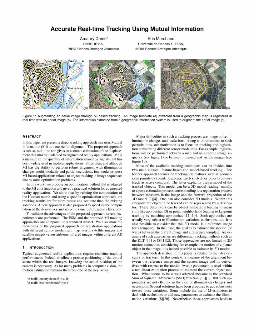
Figure 1: Augmenting an aerial image through MI-based tracking. An image template (a) extracted from a geographic map is registered inreal-time with an aerial image (b). The information extracted from a geographic information system is used to augment the aerial image (c).
ABSTRACT
In this paper we present a direct tracking approach that uses MutualInformation (MI) as a metric for alignment. The proposed approachis robust, real-time and gives an accurate estimation of the displace-ment that makes it adapted to augmented reality applications. MI isa measure of the quantity of information shared by signals that hasbeen widely used in medical applications. Since then, and althoughMI has the ability to perform robust alignment with illuminationchanges, multi-modality and partial occlusions, few works proposeMI-based applications related to object tracking in image sequencesdue to some optimization problems.
In this work, we propose an optimization method that is adaptedto the MI cost function and gives a practical solution for augmentedreality application. We show that by refining the computation ofthe Hessian matrix and using a specific optimization approach, thetracking results are far more robust and accurate than the existingsolutions. A new approach is also proposed to speed up the compu-tation of the derivatives and keep the same optimization efficiency.
To validate the advantages of the proposed approach, several ex-periments are performed. The ESM and the proposed MI trackingapproaches are compared on a standard dataset. We also show therobustness of the proposed approach on registration applicationswith different sensor modalities: map versus satellite images andsatellite images versus airborne infrared images within different ARapplications.
1 INTRODUCTION
Typical augmented reality applications require real-time trackingperformances. Indeed, to allow a precise positioning of the virtualscene within the real images, knowing the actual position of thecamera is necessary. As for many problems in computer vision, themotion estimation remains therefore one of the key issues.
∗e-mail: [email protected]†e-mail: [email protected]
Major difficulties in such a tracking process are image noise, il-lumination changes and occlusions. Along with robustness to suchperturbations, our motivation is to focus on tracking and registra-tion considering different sensor modalities. For example, registra-tions will be performed between a map and an airborne image se-quence (see figure 1) or between infra-red and visible images (seefigure 10).
Most of the available tracking techniques can be divided intotwo main classes: feature-based and model-based tracking. Theformer approach focuses on tracking 2D features such as geomet-rical primitives (point, segments, circles, etc.) or object contours(such as active contours). The latter explicitly uses a model of thetracked objects. This model can be a 3D model leading, mainly,to a pose estimation process corresponding to a registration processbetween measures in the image and the forward projection of the3D model [7][4]. One can also consider 2D models. Within thiscategory, the object to be tracked can be represented by a descrip-tor. These descriptors can be object histograms leading to meanshift like approaches [3] or point neighborhood leading to keypointtracking by matching approaches [12][10]. Such approaches areusually very robust to illumination variation, occlusions, etc. It isalso possible to consider that this 2D model is a reference image(or a template). In that case, the goal is to estimate the motion (orwarp) between the current image and a reference template. An ex-ample of such approaches are differential tracking methods such asthe KLT [13] or [8][1][2]. Those approaches are not limited to 2Dmotion estimation, considering for example the motion of a planarobject in the image, it is indeed possible to estimate its 3D motion.
The approach described in this paper is related to the later cat-egory of trackers. In this context, a measure of the alignment be-tween the reference image and the current image and its deriva-tives with respect to the motion (warp) parameters is used withina non-linear estimation process to estimate the current object mo-tion. What seems to be a well adapted measure is the standardSum of Squared Differences (SSD) function [13][1]. But such ap-proaches are not effective in the case of illumination changes andocclusions. Several solutions have been proposed to add robustnesstoward those variations. Some include the use of M-estimators todeal with occlusions or add new parameters to estimate the illumi-nation variations [8][20]. Nevertheless those approaches leads to

complex models.In this paper, our goal is first to have a visual tracking approach
that is robust to occlusions and illumination variations, but alsoto track an object with its appearance model acquired in anothermodality than the one used in the current image sequence. The pro-posed solution is then to replace the SSD function by a more robustalignment function.
One can consider local normalized cross correlation (NCC) [9]to replace SSD, but our results show that it is not applicable to dif-ferent image modalities. The proposed solution is then to max-imize the information shared between the reference image andthe sequence by maximizing the Mutual Information (MI) func-tion [19, 22, 17]. MI has also proved to be robust to occlusionsand illumination variations and can therefore be considered as agood alignment measure for tracking [6, 15]. However the existingapproaches are not taking full advantage of the accuracy of MI andthus are not appropriate for augmented reality applications.
In this paper we present a MI-based tracker where an impor-tant contribution is to propose an optimization process adapted tothe MI cost function. The optimization process that we propose isan inverse compositional approach where an important part of thederivatives needed in the optimization can be precomputed, result-ing in small computation times. A precise, complete and efficientcomputation of the Hessian matrix is described. The inverse com-positional approach allows the estimation of the Hessian matrix af-ter convergence. We show that this Hessian matrix can be used ina Newton’s like approach to give an accurate and fast estimation ofthe displacement parameters that will prove its reliability in aug-mented reality applications. Finally a new approach is proposed tospeed up the computation of the derivatives through a selection ofthe used reference pixels that makes the mutual information track-ing process possible at video-rate meeting AR requirements.
In the remainder of this paper, Section 2 presents an overviewof the differential approaches. In section 3, a brief introduction oninformation theory is given with the definition of mutual informa-tion, then a formulation adapted to the differential tracking methodis presented. Section 4 deals with the optimization of the resultingmutual information function with respect to the motion parametersto estimate. Finally section 5 presents tracking results including theMetaio benchmark and presents augmented reality experiments thatdemonstrate the new multimodal capability of the approach.
2 DIFFERENTIAL TEMPLATE-BASED TRACKING
Differential tracking is a class of approaches based on the optimiza-tion of an image registration function. The goal is to estimate thedisplacement p of an image template I∗ in a sequence of imagesI0..It . In the case of a similarity function f , the problem can bewritten as :
pt = argmaxp
f (I∗,w(It ,p)). (1)
where we search the displacement pt that maximizes the similaritybetween the template I∗ and the warped current image It . In the caseof a dissimilarity function the problem would be simply inverted inthe sense that we would search the minimum of the function f . Forthe purpose of clarity, the warping function w is here used in anabuse of notation to define the overall transformation of the imageI by the parameters p. Indeed, its correct formulation w(x,p) givesthe function that moves a point x from the reference image to itscoordinates in the current image.
The displacement parameters p can be of high dimension. Forinstance, the experiments that will be presented at the end of thepaper consider a homography transformation that corresponds top ∈ sl(3) that is 8 parameters. Approaches such as an exhaustivesearch of p are thus too expensive if not impossible.
To solve the maximization problem, the assumption made in thedifferential tracking approaches is that the displacement of the ob-ject between two consecutive frames is quite small. The previousestimated displacement pt−1 can therefore be used as first estima-tion of the current displacement to perform the optimization of fand incrementally reach the best estimation pt .
Multiple solutions exists to compute the update of the currentdisplacement parameters and perform the optimization. IndeedBaker and Matthews showed that two formulations were equiva-lent [1]. The former is the direct compositional formulation whichconsiders that the update is applied to the current image, thus wesearch the update ∆p that maximize f as:
∆pk = argmax∆p
f (I∗,w(w(It ,∆p),pk)). (2)
This equation is typically solved using a Taylor expansion wherethe update is computed with the function derivatives with respectto ∆p. The update of the current parameters pk is then applied asfollows:
w( w(x,∆p),pk) → w(x,pk+1). (3)
A second equivalent formulation is the inverse compositional for-mulation which considers that the update modifies the reference im-age, so that ∆p is chosen to maximize:
∆pk = argmax∆p
f (w(I∗,∆p),w(It ,pk)). (4)
In this case the current parameters will be updated using:
w( w−1(x,∆pk),pk) → w(x,pk+1). (5)
In the inverse compositional formulation, since the update parame-ters are applied to the reference image, the derivatives with respectto the displacement parameters will classically be computed usingthe gradient of the reference image. Thus, these derivatives can bepartially precomputed and the algorithm is far less time consuming.Since we are interested in a fast estimation of the displacement pa-rameters, the remainder of the paper will focus on the later inversecompositional approach.
One essential choice remains the one of the alignment functionf . One natural solution is to choose the function f as the sum ofsquared differences (SSD) of the pixel intensities between the ref-erence image and the transformed current image:
pt = argminp
(SSD(I∗,w(It ,p))) (6)
= argminp
∑x∈ROI
(I∗(x)− It(w(x,p)))2(7)
where the summation is computed on each point x of the referencetemplate that is the region of interest (ROI) of the reference image.As suggested by its definition, this dissimilarity function is verysensitive to occlusions and illumination variations. Many solutionshave been proposed to robustify the SSD. M-estimators robustifiesthe least squared problem toward occlusions [8] and a model of illu-mination changes can be coupled with the motion model to create atracker robust to lighting changes [20].Nevertheless those solutionsare complex since additional parameters have to be estimated andaligning two images acquired using different modalities of acquisi-tion remains impossible.
Let us for example consider an aerial image and a map template(see figure 2(a)). Considering these two modalities is obviously anextreme case, but it will emphasize the robustness of the proposedapproach. The value of SSD is computed with respect to the trans-lations between the map and the satellite image. It is clear thatthe two images are showing the same place (at least for a human

(a) (b) (c) (d)
Figure 2: Alignment functions wrt. translations between two images from the same area: (a) aerial image and the map reference. MI shows amaximum near zero translation at the alignment position whereas SSD and ZNCC gives no clear information on the alignment quality.
eye they contain the same “information”), however, since the linkbetween the intensities of the pixels is not linear, the SSD functionrepresented in figure 2(b) gives no information on the alignment be-tween the two images. The NCC has shown some very good resultsin multimodal alignment problems [9]. The efficiency of the zero-mean normalized cross correlation (ZNCC) has been evaluated onthe mutlimodal example in figure 2(c). We can see that the case istoo extreme and that there is also no significant optimum. We canconclude that even ZNCC is not sufficient to give a good measureof alignment in this case.
To deal with occlusions, illumination variations and multimodal-ity, we propose to use the mutual information [19, 22] as the align-ment function, that is, as we will see, robust to all this variations ofappearance.
3 MUTUAL INFORMATION
3.1 Information theory
Mutual information is an alignment function that was first intro-duced in the context of information theory [19]. Some essentialnotions such as entropy and joint entropy are required for a goodunderstanding of this alignment measure.
3.1.1 Entropy
Entropy h(I) is a measure of variability of a random variable I (sig-nal, image...). If r are the possible values of I and pI(r) = P(I = r)is the probability distribution function of r, then the Shannon en-tropy h(I) of a discrete variable I is given by the following expres-sion:
h(I) = −∑r
pI(r) log(pI(r)) . (8)
The log basis only changes the entropy value with a scale factor,therefore it has no interest in our tracking problem and will be omit-ted since we only seek the maximum of the cost function but not aparticular value.
Since our goal is to focus on images, let us consider I as an imageand r = I(x) as the possible gray-level intensities of the image pix-els x. The probability distribution function of the gray-level valuesis then simply given by a the normalized histogram of the image I.The entropy can therefore be considered as a measure of dispersionof the image histogram.
3.1.2 Joint entropy
Following the same principle, joint entropy h(I, I∗) of two randomvariables I and I∗ can be defined as the variability of the couple ofvariables (I, I∗). The Shannon joint entropy expression is given by:
h(I, I∗) = −∑r,t
pII∗(r, t) log(pII∗(r, t)) (9)
where r and t are respectively the possible values of the variables Iand I∗, and pII∗(r, t) = P(I = r∩ I∗ = t) is the joint probability dis-tribution function. In our problem I and I∗ are images. Then r andt are the gray-level values of the two images and the joint probabil-ity distribution function is a normalized bidimensional histogramof the two images. As for entropy, joint entropy corresponds to ameasure of dispersion of the joint histogram of (I, I∗).
At first sight the joint entropy could be considered as a goodalignment measure: if the dispersion of the joint histogram is smallthen the correlation between the two images is strong and we cansuppose that the two images are aligned. Nevertheless the depen-dencies on the entropies of I and I∗ makes it not adapted. Indeedif one of the images has a constant gray-level value then the jointhistogram would be very focused and the entropy value very smalldespite the fact that the two images are not aligned.
3.1.3 Original Mutual information
The definition of mutual information (MI) solves the above men-tioned problem [19, 22]. Subtracting the random variable’s en-tropies from their joint entropy yields to an alignment measure thatis not depending on the variable marginal entropies. The MI of tworandom variables I and I∗ is then given by the following equation:
MI(I, I∗) = h(I)+h(I∗)−h(I, I∗). (10)
MI is then the quantity of information shared between two randomvariables. If the two variables/images are aligned then their mutualinformation is maximal.
If this expression is combined with the previously defined differ-ential motion estimation problem, we can consider that the image Iis depending on the displacement parameters p. If we use the samewarp function notation as in section 2, the mutual information canthus be written with respect to p:
MI(p) = MI(w(I,p), I∗) = h(w(I,p))+h(I∗)−h(w(I,p), I∗).(11)
The final expression of MI is obtained by developing the previousequation using the entropy equations (8) and (9):
MI(p) = ∑r,t
pII∗(r, t,p) log
(pII∗(r, t,p)
pI(r,p)pI∗(t)
)(12)
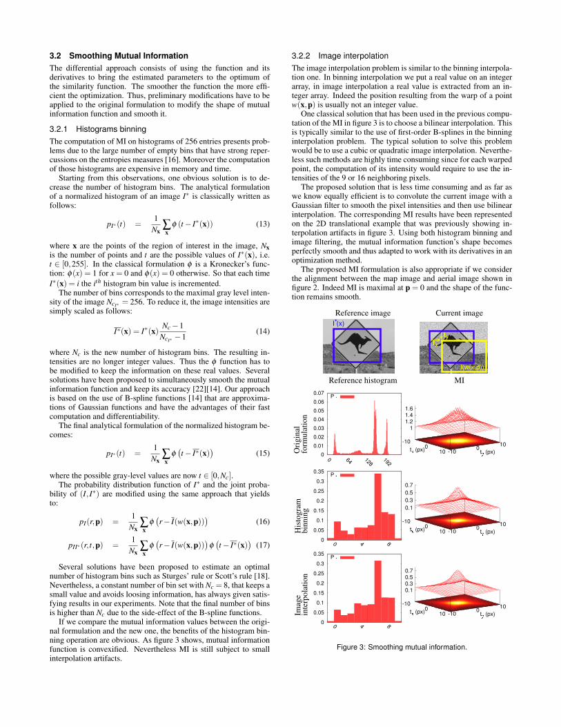
Let us consider a simple example, in figure 3 mutual informationhas been computed with respect to a translational displacement p =(tx, ty) using its classical definition. A white noise has been addedto the reference image I∗. The ground truth displacement betweenthe two images is known and is p = 0. The blue rectangle drawn inthe images represents the region of the reference image that is usedto compute the reference histograms. On the left is representedthis histogram that contains 256 gray level values. As we can see,the original definition of MI proposed by Shannon shows a largemaximum at the ground truth position but also shows many localmaxima known as interpolation artifacts.
3.2 Smoothing Mutual Information
The differential approach consists of using the function and itsderivatives to bring the estimated parameters to the optimum ofthe similarity function. The smoother the function the more effi-cient the optimization. Thus, preliminary modifications have to beapplied to the original formulation to modify the shape of mutualinformation function and smooth it.
3.2.1 Histograms binning
The computation of MI on histograms of 256 entries presents prob-lems due to the large number of empty bins that have strong reper-cussions on the entropies measures [16]. Moreover the computationof those histograms are expensive in memory and time.
Starting from this observations, one obvious solution is to de-crease the number of histogram bins. The analytical formulationof a normalized histogram of an image I∗ is classically written asfollows:
pI∗(t) =1
Nx∑x
φ (t − I∗(x)) (13)
where x are the points of the region of interest in the image, Nx
is the number of points and t are the possible values of I∗(x), i.e.t ∈ [0,255]. In the classical formulation φ is a Kronecker’s func-tion: φ(x) = 1 for x = 0 and φ(x) = 0 otherwise. So that each time
I∗(x) = i the ith histogram bin value is incremented.The number of bins corresponds to the maximal gray level inten-
sity of the image NcI∗= 256. To reduce it, the image intensities are
simply scaled as follows:
I∗(x) = I∗(x)Nc −1
NcI∗−1
(14)
where Nc is the new number of histogram bins. The resulting in-tensities are no longer integer values. Thus the φ function has tobe modified to keep the information on these real values. Severalsolutions have been proposed to simultaneously smooth the mutualinformation function and keep its accuracy [22][14]. Our approachis based on the use of B-spline functions [14] that are approxima-tions of Gaussian functions and have the advantages of their fastcomputation and differentiability.
The final analytical formulation of the normalized histogram be-comes:
pI∗(t) =1
Nx∑x
φ(t − I∗(x)
)(15)
where the possible gray-level values are now t ∈ [0,Nc].The probability distribution function of I∗ and the joint proba-
bility of (I, I∗) are modified using the same approach that yieldsto:
pI(r,p) =1
Nx∑x
φ(r− I(w(x,p))
)(16)
pII∗(r, t,p) =1
Nx∑x
φ(r− I(w(x,p))
)φ
(t − I∗(x)
)(17)
Several solutions have been proposed to estimate an optimalnumber of histogram bins such as Sturges’ rule or Scott’s rule [18].Nevertheless, a constant number of bin set with Nc = 8, that keeps asmall value and avoids loosing information, has always given satis-fying results in our experiments. Note that the final number of binsis higher than Nc due to the side-effect of the B-spline functions.
If we compare the mutual information values between the origi-nal formulation and the new one, the benefits of the histogram bin-ning operation are obvious. As figure 3 shows, mutual informationfunction is convexified. Nevertheless MI is still subject to smallinterpolation artifacts.
3.2.2 Image interpolation
The image interpolation problem is similar to the binning interpola-tion one. In binning interpolation we put a real value on an integerarray, in image interpolation a real value is extracted from an in-teger array. Indeed the position resulting from the warp of a pointw(x,p) is usually not an integer value.
One classical solution that has been used in the previous compu-tation of the MI in figure 3 is to choose a bilinear interpolation. Thisis typically similar to the use of first-order B-splines in the binninginterpolation problem. The typical solution to solve this problemwould be to use a cubic or quadratic image interpolation. Neverthe-less such methods are highly time consuming since for each warpedpoint, the computation of its intensity would require to use the in-tensities of the 9 or 16 neighboring pixels.
The proposed solution that is less time consuming and as far aswe know equally efficient is to convolute the current image with aGaussian filter to smooth the pixel intensities and then use bilinearinterpolation. The corresponding MI results have been representedon the 2D translational example that was previously showing in-terpolation artifacts in figure 3. Using both histogram binning andimage filtering, the mutual information function’s shape becomesperfectly smooth and thus adapted to work with its derivatives in anoptimization method.
The proposed MI formulation is also appropriate if we considerthe alignment between the map image and aerial image shown infigure 2. Indeed MI is maximal at p = 0 and the shape of the func-tion remains smooth.
Reference image Current image
I (x)*
I(w(x,p))
tytx
Reference histogram MI
Ori
gin
alfo
rmu
lati
on
His
tog
ram
bin
nin
gIm
age
inte
rpo
lati
on
Figure 3: Smoothing mutual information.
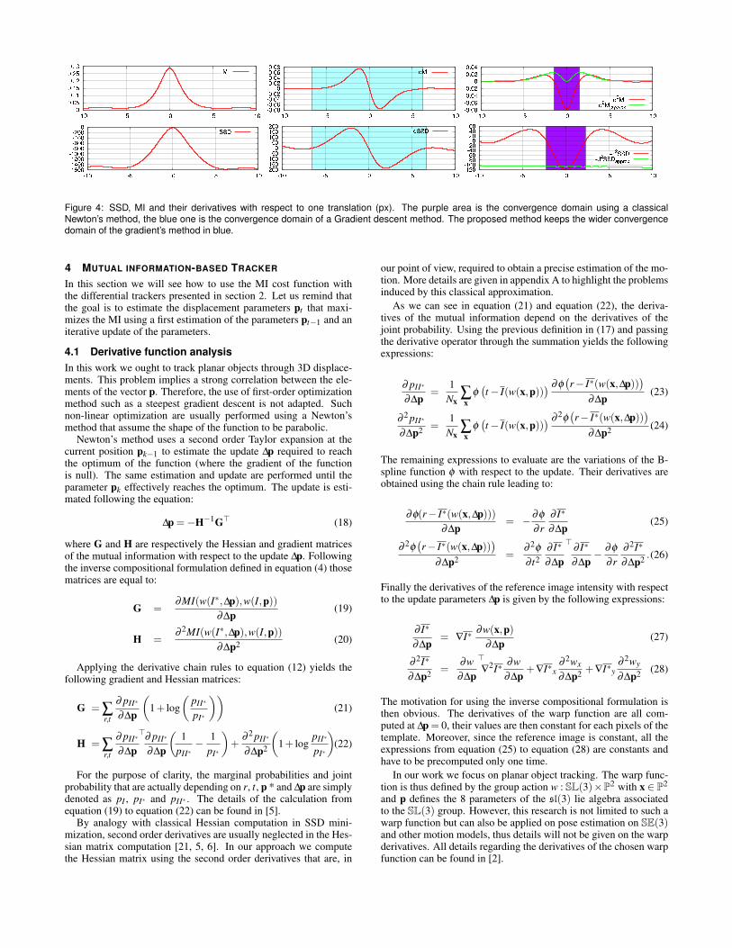
Figure 4: SSD, MI and their derivatives with respect to one translation (px). The purple area is the convergence domain using a classicalNewton’s method, the blue one is the convergence domain of a Gradient descent method. The proposed method keeps the wider convergencedomain of the gradient’s method in blue.
4 MUTUAL INFORMATION-BASED TRACKER
In this section we will see how to use the MI cost function withthe differential trackers presented in section 2. Let us remind thatthe goal is to estimate the displacement parameters pt that maxi-mizes the MI using a first estimation of the parameters pt−1 and aniterative update of the parameters.
4.1 Derivative function analysis
In this work we ought to track planar objects through 3D displace-ments. This problem implies a strong correlation between the ele-ments of the vector p. Therefore, the use of first-order optimizationmethod such as a steepest gradient descent is not adapted. Suchnon-linear optimization are usually performed using a Newton’smethod that assume the shape of the function to be parabolic.
Newton’s method uses a second order Taylor expansion at thecurrent position pk−1 to estimate the update ∆p required to reachthe optimum of the function (where the gradient of the functionis null). The same estimation and update are performed until theparameter pk effectively reaches the optimum. The update is esti-mated following the equation:
∆p = −H−1G⊤ (18)
where G and H are respectively the Hessian and gradient matricesof the mutual information with respect to the update ∆p. Followingthe inverse compositional formulation defined in equation (4) thosematrices are equal to:
G =∂MI(w(I∗,∆p),w(I,p))
∂∆p(19)
H =∂ 2MI(w(I∗,∆p),w(I,p))
∂∆p2(20)
Applying the derivative chain rules to equation (12) yields thefollowing gradient and Hessian matrices:
G = ∑r,t
∂ pII∗
∂∆p
(1+ log
(pII∗
pI∗
))(21)
H = ∑r,t
∂ pII∗
∂∆p
⊤∂ pII∗
∂∆p
(1
pII∗−
1
pI∗
)+
∂ 2 pII∗
∂∆p2
(1+ log
pII∗
pI∗
)(22)
For the purpose of clarity, the marginal probabilities and jointprobability that are actually depending on r, t, p * and ∆p are simplydenoted as pI , pI∗ and pII∗ . The details of the calculation fromequation (19) to equation (22) can be found in [5].
By analogy with classical Hessian computation in SSD mini-mization, second order derivatives are usually neglected in the Hes-sian matrix computation [21, 5, 6]. In our approach we computethe Hessian matrix using the second order derivatives that are, in
our point of view, required to obtain a precise estimation of the mo-tion. More details are given in appendix A to highlight the problemsinduced by this classical approximation.
As we can see in equation (21) and equation (22), the deriva-tives of the mutual information depend on the derivatives of thejoint probability. Using the previous definition in (17) and passingthe derivative operator through the summation yields the followingexpressions:
∂ pII∗
∂∆p=
1
Nx∑x
φ(t − I(w(x,p))
) ∂φ(r− I∗(w(x,∆p))
)
∂∆p(23)
∂ 2 pII∗
∂∆p2=
1
Nx∑x
φ(t − I(w(x,p))
) ∂ 2φ(r− I∗(w(x,∆p))
)
∂∆p2.(24)
The remaining expressions to evaluate are the variations of the B-spline function φ with respect to the update. Their derivatives areobtained using the chain rule leading to:
∂φ(r− I∗(w(x,∆p)))
∂∆p= −
∂φ
∂ r
∂ I∗
∂∆p(25)
∂ 2φ(r− I∗(w(x,∆p))
)
∂∆p2=
∂ 2φ
∂ t2
∂ I∗
∂∆p
⊤∂ I∗
∂∆p−
∂φ
∂ r
∂ 2I∗
∂∆p2.(26)
Finally the derivatives of the reference image intensity with respectto the update parameters ∆p is given by the following expressions:
∂ I∗
∂∆p= ∇I∗
∂w(x,p)
∂∆p(27)
∂ 2I∗
∂∆p2=
∂w
∂∆p
⊤
∇2I∗∂w
∂∆p+∇I∗x
∂ 2wx
∂∆p2+∇I∗y
∂ 2wy
∂∆p2(28)
The motivation for using the inverse compositional formulation isthen obvious. The derivatives of the warp function are all com-puted at ∆p = 0, their values are then constant for each pixels of thetemplate. Moreover, since the reference image is constant, all theexpressions from equation (25) to equation (28) are constants andhave to be precomputed only one time.
In our work we focus on planar object tracking. The warp func-tion is thus defined by the group action w : SL(3)×P
2 with x ∈ P2
and p defines the 8 parameters of the sl(3) lie algebra associatedto the SL(3) group. However, this research is not limited to such awarp function but can also be applied on pose estimation on SE(3)and other motion models, thus details will not be given on the warpderivatives. All details regarding the derivatives of the chosen warpfunction can be found in [2].

4.2 Optimization approach
The Newton’s method that can be used to perform the estimationof the update parameters ∆p is based on the assumption of a simi-larity function with a parabolic shape. One can immediately noticethat this assumption can be easily violated by looking at the func-tion’s shape (see figure 3). The violation could cause the Newton’smethod to fail, thus a better approach has to be chosen.
To evaluate the efficiency of the following optimization meth-ods, a set of alignment experiments has been realized. The goal isto estimate the known position p∗ of a template in an image (seefigure 5(a)) from many initial position parameters (see figure 5(b)).The initial parameters are automatically generated applying a ran-dom noise to the ground truth position.
The convergence rate of the optimization method are then evalu-ated with respect to the initial positioning error. The positioning er-ror err is defined as the RMS distance between the correct positionof some reference points x∗i = w(xi,p
∗) and the current position ofthe points w(xi,p) [11]. The reference points are simply chosen asthe 4 corners of the template so that the error becomes:
err(p) =
√√√√4
∑i=1
‖x∗i −w(xi,p)‖ (29)
We consider that the optimization converges as soon as the error erris below 0.5 px. 500 alignment experiments are performed for eachinitial positioning error err from 1 to 20 that is a total of 10000experiments. We represent the convergence rate and the averagenumber of iterations required to reach convergence. Indeed, thosevalues gives a good overview of the efficiency of the optimizationmethods.
The Gradient descent method cannot estimate an accurate esti-mation of the homography (see section 4.1). Indeed its use gives afinal estimation with an error always above 0.5 px for the all set ofexperiments (that is a 0% convergence rate). Thus the results havenot been included in figure 5.
4.2.1 Newton’s method
Mutual information function is a quasi-concave function, thus theparabolic hypothesis of the Newton’s method is only valid near theconvergence. As soon as the displacement in the sequence is im-portant, the initial parameters pt−1 would be on the convex part ofthe cost function that will cause the optimization to diverge.
The problem is in fact equivalent using a SSD function. One ex-ample of the values obtained on the estimation of a translational dis-placement is presented in figure 4 for both the MI function and theminus of the SSD function. For the purpose of clarity, we choose toanalyze the minus of the SSD function to deal with a maximizationfor both functions. The quasi-concave shape of both functions isobvious. The parabolic assumption is only correct for the concavepart of the function, that is where their second order derivatives arenegative (the area highlighted in purple). The convergence domainusing a classical Newton’s method would be very small.
As figure 5(c) shows, the convergence domain of the Newton’smethod is indeed very small in the case of the homography estima-tion. As soon as the initial error exceeds 2 px, the initial parametersare, most of the time, out of the convergence domain of the New-ton’s method and the convergence rate becomes very small.
However considering the one dimensional example, one couldexpect an optimization that has a convergence domain as wide asthe one of the gradient descent method (the blue area in figure 4).
4.2.2 Conditioning the optimization
In tracking problem formulated with a SSD function, the Gauss-Newton approximation condition the problem by estimating a Hes-sian matrix that is always definite positive (see the green curve in
Ground truth Initial positions (err = 20px)
(a) (b)
Convergence rate (%) Number of iterations
0 5 10 15 20Initial RMS error
0
20
40
60
80
100
Newton
Proposed
Fast proposed
(c)0 5 10 15 20
Initial RMS error
0
20
40
60
80
100 Newton
Proposed
Fast proposed
(d)
Figure 5: Empirical convergence analysis of the optimization meth-ods. The proposed methods (blue and green curves) have a veryhigh convergence rate compared to the classical Newton’s methods(red curve).
figure 4) and that is a good approximation of the exact Hessian ma-trix after convergence. Therefore its use permits to have a con-vergence domain as wide as the one with a gradient method (bluearea).
In the mutual information maximization, the problem is differ-ent. Indeed approximating the Hessian matrix as it is proposedin [21, 5, 6] do not gives an estimation of the Hessian matrix af-ter convergence (see the green curve in 4 for the MI function). Noapproximation on the Hessian of MI simplifies the problem as theGauss-Newton approach does for the SSD.
The solution that we propose is inspired from the Gauss-Newtonapproach. The idea remains to use an estimation of the Hessianmatrix after convergence. To compute this estimation we considerthat after convergence the alignment between the template and thewarped current image is perfect. Therefore we simply assume thatI(w(x,p)) = I∗(x).
This solution has several advantages:
• It gives a definite negative Hessian matrix that yields to havea wide convergence domain (blue area in figure 4). We cannotice that the resulting convergence domain is as wide as theone of the SSD function in the considered 1D example. Insection 5.1.2, further experiments will show that it is also thecase for a homography estimation.
• Since the Hessian matrix used in the Newton’s method is theHessian matrix after convergence, the behavior of the opti-mization near convergence is optimal and the final estimateddisplacement parameters are very accurate.
• This approach has the advantage of its computation time. Inthe classical Newton’s method the Hessian and Jacobian arecomputed for each iterations. In the proposed approach theHessian matrix is computed one time in the whole experiment.
The proposed optimization has been evaluated on the set of ex-periment presented in figure 5. As expected, the convergence do-main is larger than the one using the classical Newton’s method.The optimization converges for all the experiments with an initialerror below 16px and the convergence rate slightly decreases forerr > 16.
Figure 5(d) shows the number of iterations to reach convergence.The number of iterations with the proposed method is fewer thanthe one with the classical Newton’s method.
4.2.3 Improving the computation time
Compared to a simple least squared problem, mutual informationcan still be considered as a very complex function to compute. Theproposed approach offers already a practical solution. Nevertheless,faster performance is sometimes desired.
To compute the MI between the two images, all the informationis required, so all the reference pixels must be used to compute themarginal and joint probabilities. As for the variation of the mutualinformation computation, only the motion of the pixels that are notin a uniform region will have a strong effect. This fact is obviousfrom equation (27) and (28). One very simple modification is thento perform the computation of the gradient and Hessian using onlya selection of pixels in the template.
A simple measure to determine if a point is in a uniform region ofthe template is given by the norm of the reference image gradients.Therefore the selection condition can be written as:
‖∇I∗(x)‖ > α (30)
where α is a given threshold. The summation in equation (23) istherefore computed on the reference pixels that respect this condi-tion.
The efficiency of the proposed approach has been compared tothe previous one using the set of experiments represented in fig-ure 5. Using a threshold α = 6, the selected number of points cor-responds to 18% of the total number of reference points. We cansee on figure 5(c & d) that the convergence rate and the number ofrequired iterations is equal to the ones of the previous method up tofew percent and iterations.
In summary, for a similar efficiency, the computation time ofthe proposed method is 30% smaller. Such a selection method istherefore highly recommended in MI derivatives computation.
5 VISUAL TRACKING EXPERIMENTAL RESULTS
The visual tracking method that is presented in this paper has beenimplemented on a laptop with a 2.4GHz processor. The evalua-tion of the displacement parameters has been performed using thepresented inverse compositional scheme combined with a pyrami-dal approach that increases the convergence domain and speeds upconvergence of the optimization. We limit our experiments to theestimation of the displacement of planar objects. The estimated ho-mography can be decomposed to find the rotations and translationsof the plane and its normal up to a distance factor, which is suffi-cient for augmented reality applications.
5.1 Monomodal tracking
The robustness and accuracy of the proposed mutual informationtracker have been evaluated on various image sequences.
5.1.1 Tracking through natural variations
This experiment concerns an indoor sequence acquired at video rate(25Hz). The initialization of the tracker has been performed bylearning the reference image from the first image of the sequenceand setting the initial homography to an identity. The template in-cludes 16000 reference pixels.
The sequence has been chosen to illustrate the robustness of themotion estimation through many perturbation. Some images of thesequence are shown in figure 7. Firstly, the object is subject to sev-eral illumination variations: the artificial light produced an oscilla-tion on the global illumination of the captured sequence. Moreoverthe object is not Lambertian, thus the sequence is subject to satura-tion and specularities (see figure 7 frame 200). The object is movedfrom its initial position using wide angle and wide range motions(figure 7 frame 400). And finally the object is subject to fast motioncausing a significant blur in many images (figure 7 frame 600).
The frames of the sequence are presented with the correspondingestimated positions of the reference image. No ground truth of theobject position is known, however, the projection of the tracked im-age on the reference image has been performed and qualitatively at-tests the accuracy of the tracker. Indeed the reconstructed templatesshow strong variations in terms of appearance but not in terms ofposition. We can conclude that the estimation of the motion isrobust and accurate despite the strong illumination variations andblurring effects.
Concerning the processing time, using the proposed approachwith no selection of the reference points (section 4.2.2), the imagesare processed at video rate (25Hz). Using the fast computation (sec-tion 4.2.3) it is about 40Hz. All the corresponding sequences arepresented in the attached video.
5.1.2 Evaluation on benchmark datasets
To have a quantitative measure of its accuracy and robustness,the tracker has been evaluated on some very demanding referencedatasets proposed by Metaio GmbH [11]. Those datasets include alarge set of sequences with the typical motions that we are supposeto face in augmented reality applications. Indeed sequences usingeight reference images from low repetitive texture to highly repet-itive texture are included. And for each reference image is a set offour sequences depicting wide angle, high range, fast far and fastclose motion and one sequence with illumination variations.
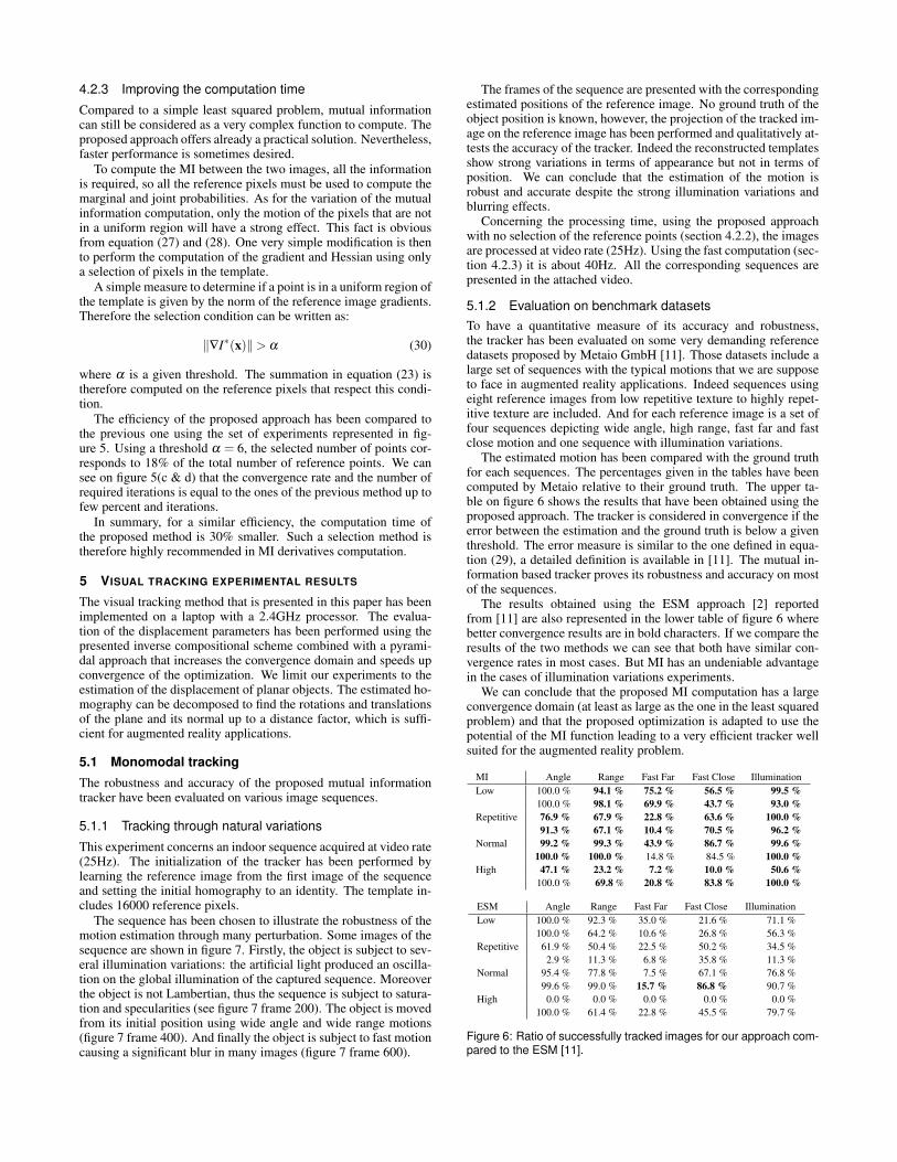
The estimated motion has been compared with the ground truthfor each sequences. The percentages given in the tables have beencomputed by Metaio relative to their ground truth. The upper ta-ble on figure 6 shows the results that have been obtained using theproposed approach. The tracker is considered in convergence if theerror between the estimation and the ground truth is below a giventhreshold. The error measure is similar to the one defined in equa-tion (29), a detailed definition is available in [11]. The mutual in-formation based tracker proves its robustness and accuracy on mostof the sequences.
The results obtained using the ESM approach [2] reportedfrom [11] are also represented in the lower table of figure 6 wherebetter convergence results are in bold characters. If we compare theresults of the two methods we can see that both have similar con-vergence rates in most cases. But MI has an undeniable advantagein the cases of illumination variations experiments.
We can conclude that the proposed MI computation has a largeconvergence domain (at least as large as the one in the least squaredproblem) and that the proposed optimization is adapted to use thepotential of the MI function leading to a very efficient tracker wellsuited for the augmented reality problem.
MI Angle Range Fast Far Fast Close Illumination
Low 100.0 % 94.1 % 75.2 % 56.5 % 99.5 %
100.0 % 98.1 % 69.9 % 43.7 % 93.0 %
Repetitive 76.9 % 67.9 % 22.8 % 63.6 % 100.0 %
91.3 % 67.1 % 10.4 % 70.5 % 96.2 %
Normal 99.2 % 99.3 % 43.9 % 86.7 % 99.6 %
100.0 % 100.0 % 14.8 % 84.5 % 100.0 %
High 47.1 % 23.2 % 7.2 % 10.0 % 50.6 %
100.0 % 69.8 % 20.8 % 83.8 % 100.0 %
ESM Angle Range Fast Far Fast Close Illumination
Low 100.0 % 92.3 % 35.0 % 21.6 % 71.1 %
100.0 % 64.2 % 10.6 % 26.8 % 56.3 %
Repetitive 61.9 % 50.4 % 22.5 % 50.2 % 34.5 %
2.9 % 11.3 % 6.8 % 35.8 % 11.3 %
Normal 95.4 % 77.8 % 7.5 % 67.1 % 76.8 %
99.6 % 99.0 % 15.7 % 86.8 % 90.7 %
High 0.0 % 0.0 % 0.0 % 0.0 % 0.0 %
100.0 % 61.4 % 22.8 % 45.5 % 79.7 %
Figure 6: Ratio of successfully tracked images for our approach com-pared to the ESM [11].

Figure 7: Tracking of a planar object through illumination variations. First row: frame 0, 200, 400 and 600. The green rectangle represents therectangle from the template image transformed using the estimated homography. Second row: projection of the templates for the same iterationsin the reference image. Third row: augmenting with a virtual robot placed on the top of the box.
5.2 Multimodal tracking
5.2.1 Satellite images versus map
This experiment illustrates the capabilities of the presented mutualinformation-based tracker in alignment applications between mapand aerial images. The reference image is a map template providedby IGN (Institut Geographique National) that can easily be linkedto Geographic Information System (GIS) and the sequence has beenacquired using a moving USB camera focusing on a poster repre-senting the satellite image corresponding to the map.
As it has been previously noticed in figure 2, a non-linear rela-tionship exists between the intensities of the map and aerial imageand this link can be evaluated by the MI functions. Mutual infor-mation can therefore allow for tracking the satellite image using themap image. Figure 9 shows the reference image and some image ofthe sequence with the corresponding overlaid results. There is noavailable ground truth for this experiment, nevertheless the overlaidresults give a good overview of the alignment accuracy. We can alsosee in the attached video that the tracker converges despite somestrong blurring effects. To validate the accuracy, we also used theestimated homography in an augmented reality application. Sincethe IGN map are linked with a GIS, some virtual information suchas road, hydrographic network, or house footprint can be overlaidon the original satellite image in a consistent way.
5.2.2 Airborne infrared image versus satellite images
The same method has been evaluated with another current modality.This time the reference is a satellite image and the sequence is anairborne infrared sequence provided by Thales Optronic. The initialhomography is manually defined.
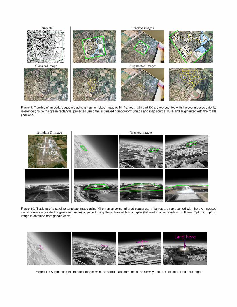
As we can expect, although very different, the two images shownin figure 10 are sharing a lot of information and thus MI can han-dle the tracking of the infrared sequence. The warp function is stilla homography. The satellite scene is then supposed to be planarleading to an approximation. Nevertheless the proposed method re-mains robust. No ground truth is available, but the overlaid images
as well as the augmented reality application qualitatively validatesthe accuracy of the tracker. As figure 10 shows, the satellite imageof the airport is well tracked on the sequence.
Figure 8: From the homography to the estimation of the camera po-sition. Green curve: estimated camera trajectory in the 3D space,blue: the 6 estimated camera positions corresponding to the framesrepresented in figure 10.
The homographies have been decomposed to estimate the po-sition of the plane with respect to the airport. The resulting 3Dtrajectory of the camera is represented in figure 8, as we can see thetrajectory is smooth and has the expected behavior that shows theapproach of a plane with respect to the runway. The trajectory of thecamera with respect to the time is presented in the attached video.Figures 10 and 11 also shows some tracked images and some aug-mented images that validate the accuracy of the motion estimation.The complete sequences are visible in the attached video.
Template Tracked images
Classical image Augmented images
Figure 9: Tracking of an aerial sequence using a map template image by MI: frames 1, 250 and 500 are represented with the overimposed satellitereference (inside the green rectangle) projected using the estimated homography (image and map source: IGN) and augmented with the roadspositions.
Template & image Tracked images
Figure 10: Tracking of a satellite template image using MI on an airborne infrared sequence. 6 frames are represented with the overimposedaerial reference (inside the green rectangle) projected using the estimated homography (Infrared images courtesy of Thales Optronic, opticalimage is obtained from google earth).
Figure 11: Augmenting the infrared images with the satellite appearance of the runway and an additional “land here” sign.

5.2.3 Potential AR applications of multimodal registration
Registering a map and an aerial image sequence is an extreme case,but registration between aerial and satellite (or any combination ofsuch modalities), acquired at different time (and thus different) canbe considered. Potential applications include visual odometry, air-craft or drone localization, pilot assistance, etc.
Infrared cameras (although still expensive) are widely used bycivilians and, obviously, military aircraft. Such a registration pro-cess with a simple satellite image may prove to be very helpful forthe pilots especially when landing (night or day) on a small and ILSfree airport. Considering that aircraft position is fully known, addi-tional information about runway, other aircraft positions or militarytargets may thus be easily displayed in the pilot helmet.
Although, we mentioned here applications in the aeronautic area,it is clear that other domains may be targeted such as energy moni-toring, robotics, urbanism, architecture, defense, ...
6 CONCLUSION
This paper presented a robust and accurate template based-trackerthat was defined using a new approach based on the mutual infor-mation alignment function. The definition of MI has been adaptedto the differential tracking problem so that the function is smoothand as concave as possible. The proposed definition preserves theadvantages of MI with respect to its robustness toward occlusions,illumination variations and images from different modalities. Anew optimization approach has been defined to deal with the quasi-concave shape of MI. The proposed approach is taking advantageof both the wide convergence domain of MI and its accurate max-imum and besides is not computationally expensive. Moreover thetime consumption is greatly reduced using a new approach basedon the reference pixels selection that yields to an accurate, fast androbust tracker suitable for augmented reality applications.
Finally the proposed tracker has been evaluated using severalexperiments. Its robustness and accuracy is verified using refer-ence datasets and shows its advantages compared with classical ap-proaches on monomodal tracking. Some new applications are alsoproposed to use a model image acquired from another modality thanthe tracked sequence that are significant in flying, for example, invehicle localization applications.
The algorithm presented here has been limited to planar objecttracking. Nevertheless the proposed approach could similarly beapplied to more complex model-based tracking applications wherewe could directly estimate the position of the object on SE(3). Themethod could also be extended to non-rigid object tracking.
APPENDIX
A WHY THE HESSIAN MATRIX MUST NOT BE APPROXI-MATED
It is common to find the Hessian matrix of MI given in equation(22) approximated by the following expression [21][5]:
H ≃ ∑r,t
∂ pII∗
∂∆p
⊤ ∂ pII∗
∂∆p
(1
pII∗−
1
pI∗
). (31)
where the second order derivative of the joint probability has beenneglected. The approximation is inspired from the one that is madein the Gauss-Newton’s method for a least squared problem that isassuming that the neglected term is null after convergence.
Considering the expression of the marginal probability pI∗(t) =∑r pII∗(r, t), it is clear that pI∗(t) > pII∗(r, t) so 1/pII∗(r, t) −
1/pI∗(t) > 0. Since∂ pII∗
∂∆p
⊤ ∂ pII∗
∂∆pis a positive matrix then the final
Hessian matrix given by (31) is positive. The goal is to maximizeMI. The Hessian matrix after convergence would then be supposedto be negative by definition. The common approximation of (31) isthus not suited for the optimization of MI.
ACKNOWLEDGMENT
This work is supported by DGA under contribution to student grant.
REFERENCES
[1] S. Baker and I. Matthews. Equivalence and efficiency of image align-
ment algorithms. In Proceedings of the 2001 IEEE Conference on
Computer Vision and Pattern Recognition, volume 1, pages 1090 –
1097, December 2001.
[2] S. Benhimane and E. Malis. Homography-based 2d visual tracking
and servoing. Int. Journal of Computer Vision, 26(7):661–676, July
2007. Special IJCV/IJRR issue on vision for robots.
[3] D. Comaniciu, V. Ramesh, and P. Meer. Real-time tracking of non-
rigid objects using mean shift. In IEEE Int. Conf. on Computer Vision
and Pattern Recognition, volume 2, pages 142–149, 2000.
[4] A. Comport, E. Marchand, M. Pressigout, and F. Chaumette. Real-
time markerless tracking for augmented reality: the virtual visual ser-
voing framework. IEEE Trans. on Visualization and Computer Graph-
ics, 12(4):615–628, July 2006.
[5] N. Dowson and R. Bowden. A unifying framework for mutual in-
formation methods for use in non-linear optimisation. In European
Conference on Computer Vision, ECCV’06, volume 1, pages 365–378,
June 2006.
[6] N. Dowson and R. Bowden. Mutual information for lucas-kanade
tracking (milk): An inverse compositional formulation. IEEE Trans.
on PAMI, 30(1):180–185, Jan. 2008.
[7] T. Drummond and R. Cipolla. Real-time visual tracking of complex
structures. IEEE Trans. on Pattern Analysis and Machine Intelligence,
24(7):932–946, July 2002.
[8] G. Hager and P. Belhumeur. Efficient region tracking with parametric
models of geometry and illumination. IEEE Trans. on Pattern Analysis
and Machine Intelligence, 20(10):1025–1039, Oct. 1998.
[9] M. Irani and P. Anandan. Robust multi-sensor image alignment. In
IEEE Int. Conf. on Computer Vision, ICCV’98, pages 959–966, Bom-
bay, India, 1998.
[10] V. Lepetit and P. Fua. Keypoint recognition using randomized trees.
IEEE Trans. on PAMI, 28(9):1465–1479, Sept. 2006.
[11] S. Lieberknecht, S. Benhimane, P. G. Meier, and N. Navab. A dataset
and evaluation methodology for template-based tracking algorithms.
In G. Klinker, H. Saito, and T. Hollerer, editors, ISMAR, pages 145–
151. IEEE Computer Society, 2009.
[12] D. Lowe. Distinctive image features from scale-invariant keypoints.
Int. Journal of Computer Vision, 60(2):91–110, 2004.
[13] B. Lucas and T. Kanade. An iterative image registration technique
with an application to stereo vision. In Int. Joint Conf. on Artificial
Intelligence, IJCAI’81, pages 674–679, 1981.
[14] F. Maes, A. Collignon, D. Vandermeulen, G. Marchal, and P. Suetens.
Multimodality image registration by maximization of mutual informa-
tion. IEEE trans. on Medical Imaging, 16(2):187–198, 1997.
[15] G. Panin and A. Knoll. Mutual information-based 3d object tracking.
Int. Journal of Computer Vision, 78(1):107–118, 2008.
[16] J. Pluim, J. Maintz, and M. Viergever. Mutual information match-
ing and interpolation artefacts. In K. Hanson, editor, SPIE Medical
Imaging, volume 3661, pages 56–65. SPIE Press, 1999.
[17] J. Pluim, J. Maintz, and M. Viergever. Mutual-information-based reg-
istration of medical images: a survey. IEEE Trans. on Medical Imag-
ing, 22(8):986–1004, Aug. 2003.
[18] D. W. Scott. On optimal and data-based histograms. Biometrika,
66(3):605–610, December 1979.
[19] C. Shannon. A mathematical theory of communication. SIGMOBILE
Mob. Comput. Commun. Rev., 5(1):3–55, January 2001.
[20] G. Silveira and E. Malis. Real-time visual tracking under arbitrary
illumination changes. In IEEE Int. Conf. on Computer Vision and
Pattern Recognition, CVPR’07, Minneapolis, USA, June 2007.
[21] P. Thevenaz and M. Unser. Optimization of Mutual Information for
Multiresolution Image Registration. IEEE trans. on Image Processing,
9(12):2083–2099, 2000.
[22] P. Viola and W. Wells. Alignment by maximization of mutual infor-
mation. International Journal of Computer Vision, 24(2):137–154,
1997.