Accurate interpolation using derivatives

Chapter 4

Accurate interpolation usingderivatives

A new technique for accurate interpolation using derivative information is pre-sented. It is a hybrid of extrapolation to arbitrary order and linear interpolation,and combines the advantages of both methods. Through a modification of thecoefficients of the Taylor expansion, extrapolations from a number of locationscan be combined to obtain a polynomial order of accuracy that is one higher thanthat of a single Taylor expansion.

The formulation of the method is very general: it can be used both in regularand irregular data distributions in spaces of arbitrary dimension. The techniqueis expected to be useful in many applications. It is used at various stages in thealgorithms described in the following chapters.

4.1 Introduction

The theory developed in Chapter 3 shows that ray field maps in position/anglecoordinates are useful tools for seismic imaging in complex media. To be relevantfor practical applications it is important that these maps are calculated efficiently.Therefore, two algorithms for the calculation of ray field maps are investigatedin Chapters 5 and 6. In preparation, this chapter introduces a new and accuratelocal interpolation technique that is used at various stages in these algorithms.

Interpolation methods approximate a function using data that are available ata distribution of data points. The data consist of the function values and possiblysome of its derivatives. The data points may be distributed in a space of arbitrarydimension. Both regular and irregular data distributions are relevant for this work,and hence both are discussed here.

Interpolation on a regular, rectangular grid is essential for the practical appli-cation of the ray field maps. In the common practice of Kirchhoff migration, for

43

44 Accurate interpolation using derivatives

example, travel time maps are first calculated on a coarse grid, but during theactual migration the travel time maps are interpolated to a denser grid (e.g., Epiliand McMechan, 1996). The main purpose of this approach is to limit storage spaceand disk traffic, because in 3-D applications the maps become far too voluminousto keep them in working memory. The more accurately the interpolation can beperformed, the more computer time is saved (e.g., Vanelle and Gajewski, 2002).

Interpolation on irregular distributions comes into play in the constructionof ray field maps. In algorithms such as wave front construction (Vinje et al.,1993; Lambare et al., 1996) and related methods (Chapters 5 and 6) ray fields arefirst calculated in terms of ray field coordinates, and subsequently mapped ontospatial coordinates. In the spatial domain the points at which the ray field isevaluated form an irregular distribution, which has to be regularised for practicalapplication. One way to perform this regularisation is by means of interpolation.Another approach, based on averaging integrals, is used in Chapter 6.

This chapter introduces a general approach to enhancing the accuracy of localinterpolation by using derivative information. The approach can be applied toboth regular and irregular data distributions in arbitrary dimension.

Interpolation methods are widely used in many fields of science. Usually clas-sical techniques as described in textbooks such as Press et al. (1992) and Ralstonand Rabinowitz (2001) are used. Recent work has been devoted to the smoothinterpolation of irregular data distributions (Sibson, 1981; Sambridge et al., 1995).The use of derivative information is usually limited to Hermite interpolation in asingle variable (Ralston and Rabinowitz, 2001) or to bi-cubic interpolation in 2-Drectangular grids (Press et al., 1992).

The method proposed here combines aspects of interpolation and extrapolation.Using the available derivatives the function is extrapolated from the data points tothe point of evaluation. Linear interpolation is used to weight the extrapolationsfrom a number of data points. The best known extrapolation formula that usesthe function values and derivatives from a single point is the Taylor expansion.Using the Taylor expansion for the extrapolation, however, can be shown to besub-optimal. Instead, a a modification of the Taylor expansion is proposed, inwhich the expansion terms are multiplied by a set of coefficients. This makes theaccuracy of the interpolation one order higher than that of each individual Taylorexpansion. Since the proposed interpolation method is a hybrid of interpolationand extrapolation the term intrapolation is coined to refer to it. The modifiedTaylor expansion is given the name Dutch Taylor expansion.

The basic principles of intrapolation and the Dutch Taylor expansion are ex-plained in Section 4.2. Application of intrapolation depends on the availability ofthe derivatives as independent data. If the derivatives are not available they can,under some accuracy conditions, be estimated from the available data. In regulargrids finite difference approximation of derivatives is adequate, as explained inSection 4.3. The accuracy and convergence rates of intrapolation are comparedto a number of alternative interpolation methods in Section 4.4.1. An example ofintrapolation in the context of ray field maps is provided in Section 4.4.2.

4.2 Accurate interpolation using derivatives 45

4.2 Accurate interpolation using derivatives

The objective of a numerical interpolation method is to approximate a functionusing data known at a set of isolated points. The data may include the functionvalues and various derivatives. In the current context only local interpolation bymeans of low order polynomials is considered. The adjective local indicates thatdata is used only from a neighbourhood of the point at which the function valueis estimated.

The general approach is to construct an interpolating function, the interpolant,which fits the available data perfectly. However, this assumes that the availabledata are exact, which in many applications is not the case. Methods exist forreducing the effect of errors by exploiting redundancy in the available data, andby relaxing the requirement of perfect fit, but these methods are inherently lesslocal and computationally more expensive.

Even in the presence of errors, local interpolation is, in many cases, the mostpractical method for approximation. It is then important to choose an interpolantthat does not enhance the errors. In case of first order (i.e. linear) interpolation theinterpolated error is bounded by the errors in the contributing data. In general,however, the risk of enhancing errors increases with increasing polynomial orderof the interpolant, especially if derivatives are used in its construction.

The reason to choose higher order interpolation may either be to enhancethe smoothness or to enhance the accuracy (Press et al., 1992). Here, the maininterest lies in enhancing the accuracy. This can be accomplished by using in-dependent derivative information or data from a larger neighbourhood. A largerneighbourhood can be used either to define interpolants with a larger support, orto obtain derivatives estimates for the data points within original support, whichcan subsequently be used to constrain the higher order interpolant. Since it ismore practical, the latter approach is followed in Section 4.3. For the remainder ofthis section it is assumed that the derivatives are known exactly or with sufficientaccuracy.

4.2.1 Interpolation of Taylor expansions

The classical approach for incorporating derivative information in interpolationschemes is to use interpolants that fit the derivatives as well as the function val-ues. Construction of such interpolants is relatively easy in 1-D (Hermite interpo-lation, e.g., Ralston and Rabinowitz, 2001), but becomes more complicated evenfor 2-D rectangular grids (e.g., Press et al., 1992). Generalisation to irregulardata distributions and to rectangular grids in higher dimensions leads to complexcalculations.

An alternative approach is to use a hybrid of extrapolation and interpolation.The function values and the available derivatives at each data point are used toconstruct an extrapolating function. At the point of evaluation the extrapolations


from neighbouring data points are then weighted with a standard linear inter-polant.

In the following it will first be shown how this hybrid strategy works for ex-trapolation using the Taylor expansion, which is the most intuitive choice forextrapolation. It turns out that for this choice the interpolation does not im-prove on the accuracy of the individual extrapolations. A major improvement isachieved by adopting another expansion that renders the order of accuracy of theinterpolation equal to its polynomial order. The approach is outlined below in1-D; generalisations to higher dimensions are discussed in Section 4.2.4.

The n-th order Taylor expansion of a function f(x) around x = ξ is given by

Tn[f(x)](x; ξ) =n∑

k=0

1

k!(x − ξ)kf (k)(ξ), (4.1)

where f (k) stands for the k-th derivative of f(x). A two-point interpolation formulabased on x0 and x1 may then be constructed as follows:

I∗n[f(x)](x;x0, x1) =

(x1 − x)

(x1 − x0)Tn[f(x)](x;x0) +

(x − x0)

(x1 − x0)Tn[f(x)](x;x1). (4.2)

This hybrid interpolation formula may in some sense be regarded as a generalisa-tion of linear interpolation. If no derivative information is available, the extrapo-lation is of zeroth order (n = 0) and the usual linear interpolation is obtained:

I∗0 [f(x)](x;x0, x1) =

(x1 − x)

(x1 − x0)f(x0) +

(x − x0)

(x1 − x0)f(x1). (4.3)

Despite its intuitive character, the interpolation of Taylor expansions has adisadvantage that is best illustrated for interpolation using first order derivatives.The Taylor expansion (4.1) is in this case a linear function, or first order poly-nomial. The interpolation of both Taylor expansions (4.2) therefore produces asecond order polynomial. It is interesting to see what second order interpolationformula (4.2) does to an arbitrary second order polynomial sampled at x0 and x1.Figure 4.1(a) clearly illustrates that the quadratic function is not reconstructed.

To understand what happens it is instructive to look at the general quadraticfunction p2(x):

p2(x) = c0 + c1x + c2x2. (4.4)

The first order Taylor expansion of this function around ξ is

T1[p2(x)](x; ξ) = p2(ξ) + (x − ξ)p′2(ξ)

= c0 + c1x + c2(2x − ξ)ξ,(4.5)


which, after some algebra, leads to the interpolant

I∗1 [p2(x)](x;x0, x1) = p2(x) + c2(x − x0)(x − x1). (4.6)

The interpolant differs from the function itself by a second order polynomial. Thisquadratic function has coefficient c2 as a multiplier, which indicates that if thiscoefficient is zero, the function is perfectly reconstructed. This is no surprise,because in that case the function is linear, and both Taylor approximations areexact.

For comparison, the result of using a standard linear interpolant is

I∗0 [p2(x)](x;x0, x1) = p2(x) − c2(x − x0)(x − x1). (4.7)

Apart from the sign, the error is exactly the same as in Equation (4.6). Hence, theuse of derivative information using Equation (4.2) does not improve the accuracyof the interpolation.

4.2.2 Intrapolation and the Dutch Taylor expansion

Here, a hybrid of extrapolation and interpolation is proposed that is similar to theTaylor-based approach of Equation (4.2), but with a major improvement in accu-racy. The interpolants are constructed in such a way that the order of accuracy isequal to the order of interpolation. In order to stress that the resulting interpola-tion formula is a hybrid of extrapolation and interpolation, the name intrapolationis introduced to refer to it. The corresponding interpolant is analogously calledthe intrapolant.

In analogy of Equation (4.2) the intrapolant is defined as

In[f(x)](x;x0, x1) =

(x1 − x)

(x1 − x0)Dn[f(x)](x;x0) +

(x − x0)

(x1 − x0)Dn[f(x)](x;x1), (4.8)

with Dn an extrapolation formula defined as

Dn[f(x)](x; ξ) =

n∑

k=0

ank

k!(x − ξ)kf (k)(ξ). (4.9)

At this point the expansion is expressed as an ansatz in terms of unknown coeffi-cients an

k , where the superscript n should be interpreted as an index rather thana power. Note that the parametric form of (4.9) reduces to the Taylor expansionwith an

k = 1.The coefficients introduced in extrapolation formula Dn provide the degrees of

freedom that can be used to force the intrapolant (4.8) to satisfy some accuracyrequirements. Since an n-th order Taylor expansion gives n-th order accuracy,interpolation of n-th order expansions is useful if it can enhance the order of


x0 x1x

p2(x)T1[p2(x)](x;x0)T1[p2(x)](x;x1)I∗

1 [p2(x)](x;x0, x1)

(a) Quadratic interpolation between points x0 and x1 based on the Taylor expansion, as inEquation (4.2). An arbitrary quadratic function is not reproduced by the interpolation.

x0 x1x

p2(x)D1[p2(x)](x;x0)D1[p2(x)](x;x1)I1[p2(x)](x;x0, x1)

(b) Quadratic interpolation between points x0 and x1 based on the Dutch Taylor expansion, asin Equation (4.21). An arbitrary quadratic function is reproduced exactly.

Figure 4.1: Approximation of a quadratic function p2(x), based on interpolation of firstorder extrapolations. For Figure (a) the extrapolation is the conventional Taylor expan-sion T , as in Equation (4.1), for Figure (b) it is the Dutch Taylor expansion D (4.9)introduced in this paper.


accuracy to n + 1. It should be noted here that the polynomial order of theintrapolant In is n+1. This means that the goal is to choose coefficients an

k in sucha way that the order of accuracy of the intrapolant is equal to its polynomial order,which is the highest order of accuracy that can be obtained. For the extrapolationformula thus obtained the term Dutch Taylor expansion is coined, for reasons thatwill become clear later on.

A general algorithm for finding coefficients in linear functionals such as (4.9)is the method of undetermined coefficients (e.g., Ralston and Rabinowitz, 2001).As a first, trivial, example determine the coefficient a0

0, that makes intrapolant(4.8) exact for first order polynomials. This should result in the well known linearinterpolant. Since any first order polynomial in x can be written as a linearcombination of the monomials 1 and x, it is sufficient to solve the system ofequations

{I0[1](x;x0, x1) = 1

I0[x](x;x0, x1) = x,(4.10)

which, using (4.8), leads to the more explicit system

a00

((x1 − x)

(x1 − x0)+

(x − x0)

(x1 − x0)

)= 1

a00

((x1 − x)

(x1 − x0)x0 +

(x − x0)

(x1 − x0)x1

)= x.

(4.11)

Although there are two equations for one coefficient the solution is consistent:

a00 = 1. (4.12)

Hence the first order intrapolant is given by

I0[f(x)](x;x0, x1) =(x1 − x)

(x1 − x0)f(x0) +

(x − x0)

(x1 − x0)f(x1), (4.13)

which is indeed equal to the usual linear interpolant.A similar system of equations can be composed to determine the coefficients

a1k for the second order intrapolant:

I1[1](x;x0, x1) = 1

I1[x](x;x0, x1) = x

I1[x2](x;x0, x1) = x2.

(4.14)

After some algebra this yields the coefficients

a10 = 1, a1

1 =1

2, (4.15)


and the intrapolant

I1[f(x)](x;x0, x1) =(x1 − x)

(x1 − x0)

[f(x0) +

1

2(x − x0)f

′(x0)

]

+(x − x0)

(x1 − x0)

[f(x1) +

1

2(x − x1)f

′(x1)

]. (4.16)

This intrapolant is exact for second order polynomials, which can be checked byinserting p2 as defined in Equation (4.4):

I1[p2(x)](x;x0, x1) = p2(x). (4.17)

Note the difference with Equation (4.6). Figure 4.1(b) shows graphically thatintrapolation with first derivatives is exact to second order.

It is not immediately obvious what the coefficients ank for the Dutch Taylor

expansion should be for higher values of n. An intrapolant that certainly haspractical relevance (e.g. Section 4.4.2) is that for n = 2, which is based on bothfirst and second derivatives. Another system of equations, similar to (4.10) and(4.14), yields coefficients

a20 = 1, a2

1 =2

3, and a2

2 =1

3. (4.18)

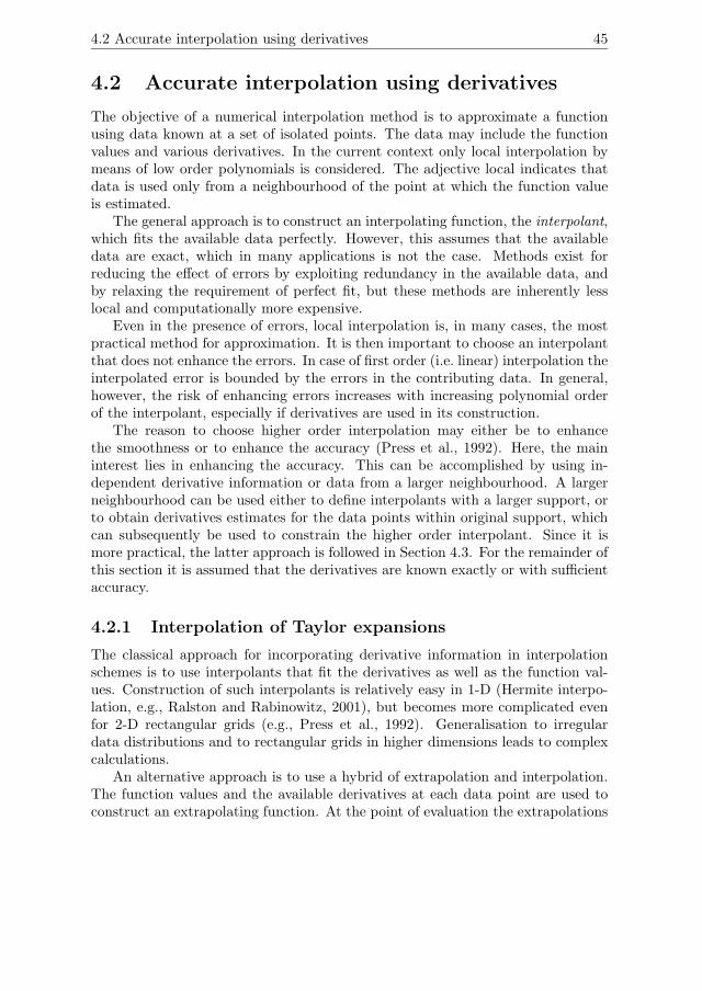
Figure 4.2 compares intrapolation of a cubic function using these coefficients withthe less accurate interpolation based on the Taylor expansion.

While the solutions for higher n are not very likely to be useful in practice(see Section 4.2.3), it is interesting to see what happens. The system of equationsgets increasingly complex and more difficult to solve, but a pattern soon becomesclear. For general n the coefficients form the series

ank =

n + 1 − k

n + 1= 1 −

k

n + 1(4.19)

where n + 1 is the polynomial order of the intrapolant, and n the maximum orderof derivatives used.

Using coefficients (4.19) the Dutch Taylor expansion (4.9) can be expressedexplicitly as

Dn[f(x)](x; ξ) =

n∑

k=0

(1 −

k

n + 1

)1

k!(x − ξ)kf (k)(ξ), (4.20)

or alternatively as a normal Taylor expansion and a correction term:

Dn[f(x)](x; ξ) = Tn[f(x)](x, ξ) −1

n + 1

n∑

k=1

k

k!(x − ξ)kf (k)(ξ). (4.21)

The correction term sums over k, starting at k = 1 simply because the argumentvanishes at k = 0. Appendix 4.A.1 proves the correctness of 4.19, by showing thatexpansion (4.21) makes the intrapolant (4.8) exact to order n + 1 for arbitrary n.


x0 x1x

p3(x)T2[p3(x)](x;x0)T2[p3(x)](x;x1)I∗

2 [p3(x)](x;x0, x1)

(a) Cubic interpolation between points x0 and x1 based on the Taylor expansion, as in Equation(4.2). A arbitrary cubic function is not reproduced by the interpolation.

x0 x1x

p3(x)D2[p3(x)](x;x0)D2[p3(x)](x;x1)I2[p3(x)](x;x0, x1)

(b) Cubic interpolation between points x0 and x1 based on the Dutch Taylor expansion, as inEquation (4.21). An arbitrary cubic function is reproduced exactly.

Figure 4.2: The equivalent of Figure 4.1, now for a cubic function p3(x), with interpola-tion based on second order extrapolations.


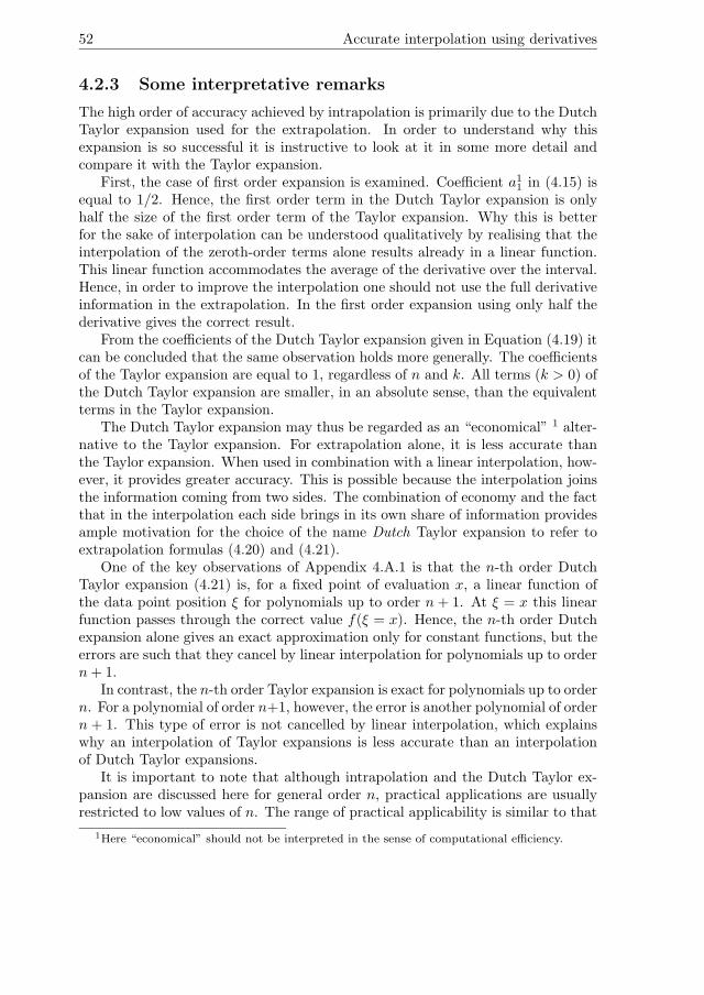
4.2.3 Some interpretative remarks

The high order of accuracy achieved by intrapolation is primarily due to the DutchTaylor expansion used for the extrapolation. In order to understand why thisexpansion is so successful it is instructive to look at it in some more detail andcompare it with the Taylor expansion.

First, the case of first order expansion is examined. Coefficient a11 in (4.15) is

equal to 1/2. Hence, the first order term in the Dutch Taylor expansion is onlyhalf the size of the first order term of the Taylor expansion. Why this is betterfor the sake of interpolation can be understood qualitatively by realising that theinterpolation of the zeroth-order terms alone results already in a linear function.This linear function accommodates the average of the derivative over the interval.Hence, in order to improve the interpolation one should not use the full derivativeinformation in the extrapolation. In the first order expansion using only half thederivative gives the correct result.

From the coefficients of the Dutch Taylor expansion given in Equation (4.19) itcan be concluded that the same observation holds more generally. The coefficientsof the Taylor expansion are equal to 1, regardless of n and k. All terms (k > 0) ofthe Dutch Taylor expansion are smaller, in an absolute sense, than the equivalentterms in the Taylor expansion.

The Dutch Taylor expansion may thus be regarded as an “economical” 1 alter-native to the Taylor expansion. For extrapolation alone, it is less accurate thanthe Taylor expansion. When used in combination with a linear interpolation, how-ever, it provides greater accuracy. This is possible because the interpolation joinsthe information coming from two sides. The combination of economy and the factthat in the interpolation each side brings in its own share of information providesample motivation for the choice of the name Dutch Taylor expansion to refer toextrapolation formulas (4.20) and (4.21).

One of the key observations of Appendix 4.A.1 is that the n-th order DutchTaylor expansion (4.21) is, for a fixed point of evaluation x, a linear function ofthe data point position ξ for polynomials up to order n + 1. At ξ = x this linearfunction passes through the correct value f(ξ = x). Hence, the n-th order Dutchexpansion alone gives an exact approximation only for constant functions, but theerrors are such that they cancel by linear interpolation for polynomials up to ordern + 1.

In contrast, the n-th order Taylor expansion is exact for polynomials up to ordern. For a polynomial of order n+1, however, the error is another polynomial of ordern + 1. This type of error is not cancelled by linear interpolation, which explainswhy an interpolation of Taylor expansions is less accurate than an interpolationof Dutch Taylor expansions.

It is important to note that although intrapolation and the Dutch Taylor ex-pansion are discussed here for general order n, practical applications are usuallyrestricted to low values of n. The range of practical applicability is similar to that

1Here “economical” should not be interpreted in the sense of computational efficiency.

4.3 Calculation of derivatives 53

of Taylor expansions. High order Taylor expansions are often used in theoreticalformulations. In practical applications, however, their use is limited because theconvergence with increasing order is typically very slow, and the region of conver-gence very small. The Dutch Taylor expansion and intrapolation are to be used insmall regions where the function to be approximated is well represented by a loworder polynomial, i.e. where the Taylor expansion coefficients decrease quickly forincreasing order.

4.2.4 Generalisation to higher dimensions

Since extrapolation to arbitrary order and first order interpolation are both welldefined in spaces of arbitrary dimension, the intrapolation method can easily begeneralised to higher dimensions.

The generalisation of the extrapolation formula is straightforward. It is definedanalogous to a multivariate Taylor expansion:

Tn[f(x)](x; ξ) =

n∑

k=0

1

k!(x − ξ)[k] : ∇[k]f(ξ), (4.22)

where x = (x1, x2, . . .)T is now a vector variable. Superscript [k] indicates the

iterated tensor product with k indices, as in

x[k] = xi1xi2 . . . xik, (4.23)

and the double dot (:) indicates contraction (summation) over all k indices. Themultivariate analogue of (4.21) is

Dn[f(x)](x; ξ) = Tn[f(x)](x; ξ) −1

n + 1

n∑

k=1

k

k!(x − ξ)[k] : ∇[k]f(ξ). (4.24)

As argued in Section 4.2.1 for intrapolation in a single dimension, the accuracyof order n+1 can be explained by the fact that the Dutch Taylor expansion (4.21) isa linear function of data point ξ for polynomials up to order n+1, passing throughthe correct value at ξ = x. The same argument holds for multiple variables.

For multivariate polynomials up to order n + 1, the Dutch Taylor expansion(4.24) yields a first order polynomial in terms of the data point variables ξ. Hence,in order to do intrapolation with an accuracy of order n + 1 any type of linearinterpolation will do. Natural generalisations of linear interpolation to higher di-mensions include the N -linear interpolation on rectangular grids, and barycentricinterpolation for general data distributions organised by N -dimensional triangu-lation. Both types of interpolation are discussed in Appendix D.

4.3 Calculation of derivatives

The interpolation methods introduced in the previous sections assume the pres-ence of derivative information on the data points. The alternative is to calculate


the derivative information from the available data. In essence this means intro-ducing data available at neighbouring data points which do not participate in theinterpolation itself.

In order to maintain the accuracy of intrapolation it is important that the ac-curacy of the derivatives match the order of the interpolating polynomial. That isto say, if the aim is a second order interpolant, which requires only first derivatives,these derivatives should be accurate to second order.

Derivative information on arbitrary data distributions can be obtained usingfinite difference (FD) methods (e.g., Fornberg, 1996, 1998). The calculation ofthese FD estimates is another example of the method of undetermined coefficients.The derivatives are expressed as a sum over neighbouring data values, multipliedby undetermined coefficients. The requirement that the derivatives are exact forpolynomials up to a given order leads to a system of equations similar to thosediscussed in Section 4.2.1.

The number of data points used in the summation, and thus the size of theneighbourhood, depends on the number of coefficients needed to parameterise apolynomial of the required order. The combination of the (relative) data locationsand the corresponding weights is called the FD stencil.

The complexity of the system of equations leading to the weights in an FDstencil strongly depends on the dimension of the data space, on the order of ac-curacy that is required, and on the geometry of the data points. A particularadvantage of rectangular, equidistant grids is that the stencils only depend onrelative data point positions, which means that the same stencil can be used foralmost every data point in the grid. Only the grid points near the edges requireadapted stencils.

In arbitrary data distributions the situation is a lot more complicated. Thedefinition of a neighbourhood around a data point is much less obvious, and therelative positions of neighbouring data points change from place to place. Theresult is that each data point requires a dedicated FD stencil to obtain accuratederivatives. For most practical applications, including ours, this is computationallytoo expensive.

If the objective for the calculation of derivatives is smooth rather than accurateinterpolation, one can think of many alternatives for the calculation of reasonablederivative estimates (e.g., Sibson, 1981). The author is, however, not aware of apractical approach that meets the accuracy requirements. For irregular data dis-tributions it is assumed that the derivative information is independently available.

Centred finite differences

In the following the calculation of low order FD estimates in equidistant gridsis summarised. The derivations are not be discussed here but can be found forexample in Fornberg (1996, 1998). First, consider the one dimensional FD estimatefor the derivative f ′(x) of a function f(x). A three-point centred FD is exact for

4.3 Calculation of derivatives 55

polynomials up to second order:

f ′(x) =f(x + h) − f(x − h)

2h+ O(h2). (4.25)

The coefficient multiplying f(x) itself happens to be equal to zero, which effectivelymakes it a two-point formula.

The second derivative estimate requires all three function values:

f ′′(x) =f(x + h) − 2f(x) + f(x − h)

h2+ O(h2). (4.26)

This formula is actually exact for polynomials up to third order, due to the sym-metry of the FD stencil. This suggests the use of three-point centred FD for thirdorder accurate intrapolation. The first order derivatives obtained using (4.25),however, are only accurate to second order. The application of (4.25) to a thirdorder monomial cx3 yields

c(x + h)3 − c(x − h)3

2h= 3cx2 + ch2. (4.27)

This shows that the three-point centred FD estimate of the first derivative of anythird order polynomial is wrong by a constant value. Fortunately, the intrapolant(4.8) only depends on the difference of the first derivatives at the two data points.This can be seen by looking at the interpolation of the first order expansion termsonly:

an1

(x1 − x)

(x1 − x0)(x − x0)f

′(x0) + an1

(x − x0)

(x1 − x0)(x − x1)f

′(x1)

= an1

(x − x0)(x − x1)

(x1 − x0)(f ′(x1) − f ′(x0)) (4.28)

This means that the constant is cancelled in the interpolant, and it is indeed pos-sible to do third order accurate interpolation using only three-point FD estimates.

One-sided finite difference formulas

At the boundaries of a grid it is necessary to compute the derivatives using one-sided rather than centred FD formulas. Depending on the desired order of accuracythe following formulas are available (from Fornberg, 1996, table 3.1-2):

f ′(x) =−f(x) + f(x + h)

h+ O(h) (4.29)

=−3f(x) + 4f(x + h) − f(x + 2h)

2h+ O(h2) (4.30)

=−11f(x) + 18f(x + h) − 9f(x + 2h) + 2f(x + 3h)

6h+ O(h3), (4.31)


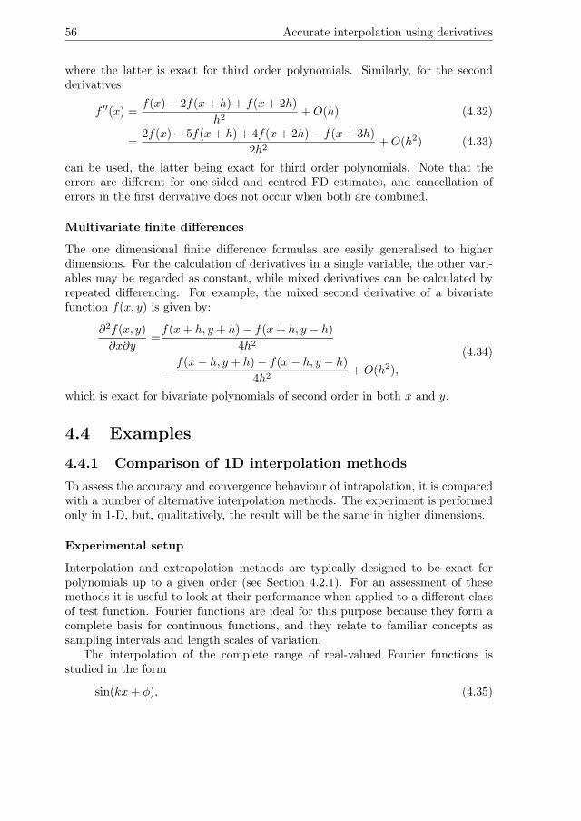
where the latter is exact for third order polynomials. Similarly, for the secondderivatives

f ′′(x) =f(x) − 2f(x + h) + f(x + 2h)

h2+ O(h) (4.32)

=2f(x) − 5f(x + h) + 4f(x + 2h) − f(x + 3h)

2h2+ O(h2) (4.33)

can be used, the latter being exact for third order polynomials. Note that theerrors are different for one-sided and centred FD estimates, and cancellation oferrors in the first derivative does not occur when both are combined.

Multivariate finite differences

The one dimensional finite difference formulas are easily generalised to higherdimensions. For the calculation of derivatives in a single variable, the other vari-ables may be regarded as constant, while mixed derivatives can be calculated byrepeated differencing. For example, the mixed second derivative of a bivariatefunction f(x, y) is given by:

∂2f(x, y)

∂x∂y=

f(x + h, y + h) − f(x + h, y − h)

4h2

−f(x − h, y + h) − f(x − h, y − h)

4h2+ O(h2),

(4.34)

which is exact for bivariate polynomials of second order in both x and y.

4.4 Examples

4.4.1 Comparison of 1D interpolation methods

To assess the accuracy and convergence behaviour of intrapolation, it is comparedwith a number of alternative interpolation methods. The experiment is performedonly in 1-D, but, qualitatively, the result will be the same in higher dimensions.

Experimental setup

Interpolation and extrapolation methods are typically designed to be exact forpolynomials up to a given order (see Section 4.2.1). For an assessment of thesemethods it is useful to look at their performance when applied to a different classof test function. Fourier functions are ideal for this purpose because they form acomplete basis for continuous functions, and they relate to familiar concepts assampling intervals and length scales of variation.

The interpolation of the complete range of real-valued Fourier functions isstudied in the form

sin(kx + φ), (4.35)

4.4 Examples 57

where x is the variable to be interpolated, k the frequency (or wave number) andφ an arbitrary phase shift.

Without loss of generality the first data point may be chosen at x0 = 0 (NBarbitrary phase shifts are accommodated by φ), and the second data point at x1 =1, because variations in the width of the data point interval are mathematicallyequivalent to variations in k. In this light k may be interpreted as a relativefrequency that can be expressed as a product of the absolute frequency k and thewidth of the interpolation interval h:

k = kh. (4.36)

Variations in k may thus be attributed to variations in interval width (h), or to

variations in absolute frequency (k).For an arbitrary interpolant I, the error E may be expressed as a function of

k, x, and φ:

E(k, x, φ) = I [sin(kx + φ)](x, 0, 1) − sin(kx + φ). (4.37)

For fixed frequency k and fixed position x the error is a periodic function of φ.To obtain insight in the behaviour of the error as a function of k and x, the RMSaverage over the range of φ is calculated:

[Erms

φ (k, x)]2

=1

2π

2π∫

0

[E(k, x, φ)]2dφ. (4.38)

To isolate the frequency dependence the error is averaged over the range of x:

[Erms

xφ (k)]2

=1

2π

1∫

0

2π∫

0

[E(k, x, φ)]2dφdx. (4.39)

The error functions are calculated for a number of different interpolation methods.

Interpolation methods

The interpolation methods discussed here are subdivided into three groups. Thefirst group consists of the intrapolation methods In (4.8), for n = 0, 1, 2. Thederivatives used in the extrapolation may either be exact or obtained by finitedifference. For the FD estimators an equidistant grid is assumed, which meansthat data points at x = −1 and x = 2 come into play. In total, five differentintrapolation methods are tested.

The second group consists of two variations of Hermite interpolation: oneusing exact and one using FD derivatives. In two-point Hermite interpolation (e.g.,Ralston and Rabinowitz, 2001) a third order polynomial interpolant is constructed


that fits both the function values and its first derivatives exactly. The Hermiteinterpolant for a function f(x) may be expressed as

IH [f(x)](x, 0, 1) = f(0)a0(x) + f(1)a1(x) + f ′(0)b0(x) + f ′(1)b1(x), (4.40)

with basis functions a0(x), a1(x), b0(x), and b1(x) defined by

a0(x) = 2x3 − 3x2 + 1, (4.41)

a1(x) = −2x3 + 3x2, (4.42)

b0(x) = x3 − 2x2 + x, and (4.43)

b1(x) = x3 − x2, (4.44)

Two-point Hermite interpolation does not have a simple analogue in dimensionshigher than one.

The third group are nearest neighbour interpolations INn . In fact, these are

Taylor expansions from the data point that is nearest to the point of interpolation:

INn [f(x)](x, 0, 1) =

{Tn[f(x)](x, 0) for 0 ≤ x < 1

2

Tn[f(x)](x, 1) for 12 ≤ x ≤ 1.

(4.45)

Nearest neighbour interpolations are also studied for n = 0, 1, 2. The latter twouse derivatives that can either be exact or FD estimates, which makes a totalof five different nearest neighbour interpolants. Nearest neighbour interpolationwith n = 2 and FD derivatives is used by Vanelle and Gajewski (2002) for theinterpolation of travel time maps (see Section 4.4.2).

Results

For all types of interpolation, the error functions (4.37) to (4.39) can be calculatedanalytically. The error curves in Figures 4.3- 4.5 are made using high precisionarithmetic in Mathematica.

Figure 4.3 shows the phase shift averaged error (4.38) for a fixed frequency of0.1 as a function of x. For each type of interpolation a single line style is chosen;the distinction between different orders for intrapolation and nearest neighbourinterpolation is easily made from the height of the curves. (The lowest curverepresents the smallest error and corresponds to the highest order.)

Due to the symmetry of the interpolations, all error curves are symmetricalabout x = 0.5. Most of the curves, viz. those that represent an interpolation thatuses derivatives, are coloured differently on the left and the right side of the graph.Black and grey make a distinction between the methods that use exact derivatives(black on the left side, grey on the right), and those that use FD derivatives (greyon the left, black on the right).

For the more accurate interpolations (lower curves) it obvious that using exactderivatives yield a higher accuracy then FD derivatives. If derivatives are avail-able, Hermite interpolation and third order intrapolation (n = 2) contend for the

4.4 Examples 59

-14

-12

-10

-8

-6

-4

-2

0

0 0.1 0.2 0.3 0.4 0.5 0.6 0.7 0.8 0.9 1

10lo

gE

rms

φ(0

.1,x

)

x

Intrapolation n = 0, 1, 2Hermite interpolationNearest neighbour interpolation n = 0, 1, 2

Figure 4.3: The RMS error made in the interpolation of a sine (4.35) with frequencyk = 0.1, averaged over the full range of possible phase shifts (4.38). All curves aresymmetric about x = 0.5. Some curves, however, are plotted black on one side, and greyon the other; curves that are black on the left side use either no or exact derivatives,those that are black on the right side use either no or FD derivatives. The line stylesof different orders n of an interpolation type are the same, but the lowest curves (leasterror) correspond to the highest order.

-16

-14

-12

-10

-8

-6

-4

-2

0

2

-3 -2.5 -2 -1.5 -1 -0.5 0 0.5 1

10lo

gE

rms

φx

(k)

10 log k

Intrapolation n = 0, 1, 2Hermite interpolation

Nearest neighbour interpolation n = 0, 1, 2

Figure 4.4: The RMS error of interpolating sines (4.35) as a function of frequency,averaged over the full range of possible phase shifts and over the range of x (4.39). Thevalues at 10 log k = −1 correspond to the RMS averages of the curves of Figure 4.3. Boldblack curves correspond to interpolation types that use either no or exact derivatives,while grey curves use FD estimates. The plot clearly indicates the different rates ofconvergence for the different interpolation types, as well as their relative RMS accuracy.


-1

0

1

2

3

4

-3 -2.5 -2 -1.5 -1 -0.5 0 0.5 1

d10lo

gE

rms

φx

(k)/

d10lo

gk

10 log k

Intrapolation n = 0, 1, 2Hermite interpolationNearest neighbour interpolation n = 0, 1, 2

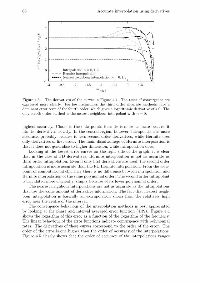
Figure 4.5: The derivatives of the curves in Figure 4.4. The rates of convergence areexpressed more clearly. For low frequencies the third order accurate methods have adominant error term of the fourth order, which gives a logarithmic derivative of 4.0. Theonly zeroth order method is the nearest neighbour interpolant with n = 0.

highest accuracy. Closer to the data points Hermite is more accurate because itfits the derivatives exactly. In the central region, however, intrapolation is moreaccurate, probably because it uses second order derivatives, while Hermite usesonly derivatives of first order. The main disadvantage of Hermite interpolation isthat it does not generalise to higher dimension, while intrapolation does.

Looking at the lowest error curves on the right side of the graph, it is clearthat in the case of FD derivatives, Hermite interpolation is not as accurate asthird order intrapolation. Even if only first derivatives are used, the second orderintrapolation is more accurate than the FD Hermite interpolation. From the view-point of computational efficiency there is no difference between intrapolation andHermite interpolation of the same polynomial order. The second order intrapolantis calculated more efficiently, simply because of its lower polynomial order.

The nearest neighbour interpolations are not as accurate as the intrapolationsthat use the same amount of derivative information. The fact that nearest neigh-bour interpolation is basically an extrapolation shows from the relatively higherror near the centre of the interval.

The convergence behaviour of the interpolation methods is best appreciatedby looking at the phase and interval averaged error function (4.39). Figure 4.4shows the logarithm of this error as a function of the logarithm of the frequency.The linear behaviour of the error functions indicate convergence with polynomialrates. The derivatives of these curves correspond to the order of the error. Theorder of the error is one higher than the order of accuracy of the interpolations.Figure 4.5 clearly shows that the order of accuracy of the interpolations ranges

4.4 Examples 61

from 0 to 3.In both convergence plots the black lines correspond to the interpolation meth-

ods that use exact derivatives, while the grey lines correspond to those that use FDderivative estimates. The intrapolations and the nearest neighbour interpolationsshow the expected convergence behaviour. In general, the order of accuracy of thenearest neighbour interpolations are equal to the order of the derivatives that areused. For the intrapolations, the order of accuracy is always one higher than theorder of derivatives (n) used.

Hermite interpolation with exact derivatives shows the expected result of be-ing accurate to third order. If FD estimates are used for the derivatives, however,Hermite interpolation turns out to be accurate only to second order, because theFD estimates themselves are only accurate to second order (4.25). For intrapo-lation the latter does not pose a limitation on the order of accuracy because ofthe fortuitous cancellation of errors discussed in Section 4.3. Even intrapolationbased only on first order FD derivatives (n=1) is slightly more accurate than FDHermite interpolation, while both methods use the same data.

If no exact derivatives are available, intrapolation should be preferred overHermite interpolation. Also, if both first and second order exact derivatives areavailable, Figure 4.4 indicates that intrapolation is the method of choice for inter-polation, because it gives the lowest error curve in the plot. If only first order exactderivatives are known Hermite interpolation is preferred. In higher dimensions,however, Hermite interpolation is not available. Finally, intrapolation is always tobe preferred over nearest neighbour interpolations.

4.4.2 Travel time interpolation

An important application of interpolation in the context of this thesis is the in-terpolation of travel time maps for Kirchhoff-type imaging. Coarse gridded traveltime maps in depth are commonly calculated for the full range of source and re-ceiver locations, prior to the actual imaging. Upon imaging these coarse maps areinterpolated to a finer grid. Higher order accuracy in the interpolation allows forcoarser maps to start with, which saves storage space and data traffic overhead inpractical implementations.

The advantages of travel time interpolation with higher order accuracy wereshown by Vanelle and Gajewski (2002). They proposed the second order (n = 2)nearest neighbour interpolant discussed in Section 4.4.1, using FD estimates ofthe derivatives. Here, it is shown that using the same amount of information agreater accuracy can be achieved using intrapolation. The second order methodproposed by Vanelle and Gajewski (2002) may therefore be replaced by thirdorder intrapolation, which enhances the advantages at negligible additional cost.Another advantage is that the interpolated travel times are continuous.

To demonstrate that intrapolation works in higher dimensions, a single exampleof travel time interpolation in a regular grid is shown here. Other examples willbe provided in later chapters.


-0.5 0.5x

-0.5

0.5

z

(a) Rays and wave fronts

-0.5 0.5x

-0.5

0.5

z

(b) Contours of squared travel time

Figure 4.6: Figure (a) shows the rays and wave fronts in a medium with V satisfyingV −2 = 1 − z. The grey tones in the background indicates the velocity (darker meansfaster). Figure (b) shows a contour plot of the corresponding squared travel time. On topa rectangular grid of points is drawn, which contain the data used in the interpolation

-14

-12

-10

-8

-6

-4

-2

0

0.5 1 1.5 2 2.5 3

RM

Ser

ror

at10

00poi

nts

log N

Intrapolation n = 0, 1, 2Nearest neighbour interpolation n = 0, 1, 2

Figure 4.7: Convergence of RMS interpolation error for the square of travel time at 1000random samples in the domain of figure 4.6. The number N corresponds to the numberof grid intervals in both dimensions. Each interpolation type has three curves, arrangedin increasing order from top to bottom.

4.5 Discussion and conclusions 63

Vanelle and Gajewski (2002) argue that it is better to interpolate the squareof the travel time (hyperbolic interpolation) than the travel time itself (parabolicinterpolation), because in a homogeneous medium the square of the travel timeis a quadratic function of the position relative to the source. Hence, in a ho-mogeneous medium any interpolation method of second or higher order accuracywill reconstruct the squared travel time perfectly. In inhomogeneous media, theinterpolation will not be exact anymore, but close to the source the hyperbolicinterpolation will always be superior.

The travel time map to be interpolated is one that can be obtained analyticallyfrom the analytic ray solution. The medium, shown in Figure 4.6(a), along witha number of rays and wave fronts emitted by a point source in the origin, has aconstant gradient of the square of the slowness (reciprocal velocity) of magnitude1, and velocity of 1 at the origin. Figure 4.6(b) shows some contours of the squaredtravel time, as well as an example of a rectangular grid defined in the medium.

Because the travel times on the grid are calculated analytically, the grid spacingdetermines the accuracy of interpolation. For a range of grid spacings, the RMSinterpolation error is calculated from a set of 1000 random locations. For N thenumber of grid intervals in each dimension the error is plotted in Figure 4.7.

As in Section 4.4.1, the nearest neighbour interpolations as well as the intrap-olations show the expected convergence rates. Intrapolation based on first andsecond order derivatives (n = 2) proves to be the most accurate. Surprisingly,even intrapolation with only first order derivatives (n = 1), is more accurate thanthe nearest neighbour interpolation that uses both first and second derivatives.

In practical applications one is usually less interested in the order of conver-gence of a given interpolation method then in the grid spacing corresponding to agiven error. The results of Figure 4.7 can be fitted with linear functions. In thisway the number of grid intervals needed for each interpolation method to obtainan acceptable error of, say 10−4 can be deduced. Rounded to the first integerabove, this gives 60, 6, and 5 for intrapolation with n = 0, 1, 2, respectively, and2393, 46, and 11 for the respective nearest neighbour interpolations. The higherthe desired accuracy, the greater the advantage of intrapolation.

4.5 Discussion and conclusions

A new technique for accurate interpolation using derivative information is pre-sented. The technique is called intrapolation, because it is a hybrid of linearinterpolation and extrapolation. The extrapolation is done by a modification ofthe Taylor expansion, referred to as the Dutch Taylor expansion. The order of ac-curacy of intrapolation is one higher than that of an individual Taylor expansionthat uses the same amount of derivative information.

Intrapolation is generally applicable in spaces of arbitrary dimension, in reg-ular as well as irregular data distributions. For interpolation inside an irregulardata distribution, the presence of a geometric structure such as an N -dimensional


triangulation is assumed. For interpolation in rectangular grids, intrapolation mayalso be applied without the presence of independent derivative information. In-stead, finite difference estimates for the derivatives may be used. Using only threepoint FD stencils, an interpolation of third order accuracy is obtained.

Intrapolation does not attempt to fit the available derivative data perfectly. Itonly uses this data to “steer” the interpolant in the right direction, resulting inan enhanced accuracy. It should be noted, however, that the derivatives are ingeneral discontinuous across the edges of the interpolants. If smoothness ratherthan accuracy is the reason for higher order interpolation it will be advisable touse a different method (e.g., Press et al., 1992; Sambridge et al., 1995).

An important advantage of not attempting to fit the derivatives perfectly isthat it is not necessary to use high polynomial orders for the interpolants. Higherorder polynomials are more expensive to evaluate, and are more sensitive to errorsin the data. In intrapolation, the influence of the derivatives at all of the datapoints is (in a way) averaged – note the reduced size of the coefficients in the DutchTaylor expansion – and therefore the interpolants are less sensitive to errors andmore stable than methods that fit the derivatives perfectly.

In order to check the accuracy of intrapolation the method is subjected totwo tests. The first test in a 1-D setting shows that the theoretical order ofaccuracy is indeed obtained in practice. For two-point interpolation, intrapolationoutperforms all other interpolation methods. Only if the first derivatives are knownexactly, Hermite interpolation yields a third order accuracy, while intrapolationneeds second derivatives as well to improve on that. In higher dimensions, however,Hermite interpolation is not available.

The second test involves the interpolation of travel times for a point source in2-D, where intrapolation is tested against nearest neighbour interpolation, bothusing FD derivative estimates. It turns out that in this case intrapolation usingonly a single derivative already outperforms the nearest neighbour interpolationthat uses second derivatives as well.

It seems fair to conclude that intrapolation is a very attractive method foraccurate interpolation both for regular and – if independent derivative data isavailable – for irregular data distributions. Implementation is straightforward.The method should be useful in a wide variety of applications. Examples of its usein ray field calculations are provided in Chapter 5, while the applicability of theDutch Taylor expansion in a broader context is further investigated in Chapter 6.

4.A Appendix

4.A.1 Dutch Taylor expansion coefficients

The intrapolant of polynomial order n + 1 is constructed using the the functionderivatives up to order n. This appendix provides the proof that the Dutch Taylorexpansion coefficients an

k , as stated in Equation (4.19), render the intrapolant (4.8)

4.A Appendix 65

exact for polynomials up to order n + 1.Point of departure is the Dutch Taylor expansion 4.21. For a given function

f(x), and a data point ξ at which the derivatives up to order n are known, thisformula gives the extrapolated value as a function of the point of evaluation x.

Alternatively one can interpret (4.21) as a function of ξ, for a fixed point ofevaluation x. This perspective is very useful here, because it clearly shows theconditions under which the intrapolant (4.8) is exact. Since the intrapolant isdefined as a linear interpolation, it is exact if and only if extrapolation formula(4.21) is a linear function of data point ξ, passing through the correct value atξ = x. Here it is shown that this is the case for polynomials up to order n + 1.The proof is divided in two parts, one for polynomials up to order n, and one forthe polynomial of order n + 1. First, however, some binomial identities are shownthat are useful in the derivations.

Binomial identities

The binomial ’n over k’ is defined as(

n

k

)=

n!

(n − k)!k!. (4.46)

The binomial occurs in the expansion of the n-th power of a sum:

(A + B)n =

n∑

k=0

(n

k

)AkBn−k. (4.47)

This relation will be used in the form

n∑

k=0

(n

k

)(x − ξ)kξn−k = xn. (4.48)

Finally,

k

(n

k

)= n

(n − 1

k − 1

)(4.49)

is another binomial identity that will be used.

Proof for polynomials of order m ≤ n.

For a monomial xm, with 0 ≤ m ≤ n, the n-th order Taylor expansion is exact, sothe extrapolation formula (4.21) becomes

Dn[xm](x; ξ) = xm −1

n + 1

m∑

k=1

k

(m

k

)(x − ξ)kξm−k, (4.50)


where the limit of the sum has changed from n to m, simply because higher termsare zero.

Using binomial identity (4.49) and the index K = k − 1 gives

Dn[xm](x; ξ) = xm −m

n + 1

m−1∑

K=0

(m − 1

K

)(x − ξ)K+1ξm−1−K

= xm −m

n + 1(x − ξ)

m−1∑

K=0

(m − 1

K

)(x − ξ)Kξm−1−K .

(4.51)

Application of (4.48) finally leads to

Dn[xm](x; ξ) = xm −m

n + 1(x − ξ)xm−1

=

(1 −

m

n + 1

)xm +

m

n + 1xm−1ξ.

(4.52)

The extrapolation formula is apparently a linear function of data point ξ for poly-nomials up to order n, while it has the exact value xm for ξ = x. Hence, theintrapolant is exact at least up to order n.

Proof for polynomial of order n + 1

For a monomial xn+1 the n-th order Taylor expansion is no longer exact, but theerror is easy to find:

Tn[xn+1](x; ξ) = xn+1 − (x − ξ)n+1. (4.53)

The Dutch Taylor expansion becomes

Dn[xn+1](x; ξ) = xn+1 − (x − ξ)n+1

−

n∑

k=1

k

n + 1

(n + 1

k

)(x − ξ)kξn+1−k. (4.54)

Using binomial identities (4.48) and (4.49), and the index K = k−1 this expressioncan be simplified to

Dn[xn+1](x; ξ) = xn+1 − (x − ξ)n+1 −

n−1∑

K=0

(n

K

)(x − ξ)K+1ξn−K

= xn+1 − (x − ξ)n+1 − (x − ξ) [xn − (x − ξ)n]

= xnξ.

(4.55)

Again, this is an expression that is linear in ξ. In fact, it is of the same formas the expression obtained for lower order polynomials in Equation (4.52), withm = n + 1. Linear interpolation of this expression using the intrapolant (4.8)indeed returns the exact polynomial xm for 0 ≤ m ≤ n+1. Hence, the intrapolantis accurate to order n + 1.

Documents

Accurate interpolation using derivatives