1

Accuracy/Precision/General Error Conceptsp

CSS 455, Winter 2012Scientific Computing

Errata: chapter 1 of turner

• P3, 2nd equation: last term should be a-mβ-m

rather than a-mβm

• P3, Eq 1.3, last term should be bNβ-N rather q Nβthan bNβN

• P11, Exercise 3. third term in cosh(x) should be (x4/4!) rather that (x4/41)

• P282, Section 1.4, last answer (1.67618) is incorrect.

Precision

• Precision refers to the number of significant figures or to the repeatability of the measurement Precision may bethe measurement. Precision may be improved by larger data sets.

• (For example, 6.022x1023 is a more precisemeasurement of Avogadro’s Number than is 6.02x1023.)

2

• Accuracy is an indication of how close the measurement is to the true value. It may include systematic instrument error.

Accuracy

y• For example, 6.0 x1023 is a more accurate value of

Avogadro’s Number than is 5.885646x1023.

Computational Error

• Algorithmic Error:Truncation or discretization. Some terms may be omitted. For example, Taylor Series for a f nction:function:

+′′′

+′′

+′+=+ )(!3

)()(!2

)())(()()( 32 δδδδ xfxfxfxfxf

We may truncate after just a few terms for small δ

Computational Error

• Data representationRounding. Computer representation of real numbers is generally inexact. – (The number 1/3 will be rounded to 0.3333333 in some

floating point representations.)

• Error Propogation.Calculations are often done in steps. The later steps depend upon the results (and errors) of the earlier ones.

3

Error Analysis

• Absolute: approximate - true. – Units are the same as the measured values.

• Relative: Absolute error divided by true value.

truetrueapprox −

Unitless, expressed as fraction or percent.

Floating-Point Numbers• Many scientific calculations are done with

approximately 64 bits used for floating point representation: real*8, double precision (most workstations)

• The division of these bits between exponent and mantissa fields varies from machine to machine. The precision is about 14-16 decimal digits and the exponent range is about 10±200 - 10 ±500

DU>> format long eEDU>> n=2/3n =

6.666666666666666e-001

Double Precision is default on Matlab. Single precision and integer representation must be selected.

Floating Point RepresentationUELbbbbbx E

N ≤≤×±= with , β. 3210 …

•β is the base (β=2 in binary system)

•b0 is implicit digit (defined by convention) (b0=1)0 p g ( y ) ( 0 )

•b1b2…bN is the mantissa field of N-digits

•E is the exponent field

ENNbbbbbx β

β...

βββ 33

221

0⎭⎬⎫

⎩⎨⎧ +++++±=

4

Normalized Binary Representation

( ) ( ) ( ) ( ) ( ) ( ) 1216212120202119 0123410 ++=++++=

4420011.1.10011 ×=

Implicit bit

Normalized Binary Representation

( ) ( ) ( ) ( ) ( ) ( ) ( ) ( ) …++++++++=⎟⎠⎞

⎜⎝⎛ 8

217

216

215

214

213

212

21

21

10

1100110051

⎞⎛ …… 11000011001100.02561

1281

161

81

51

10

=++++=⎟⎠⎞

⎜⎝⎛

3

10

201001100110.151 −×=⎟⎠⎞

⎜⎝⎛ …

Implicit bit

Parameters for typical floating-point systems

System β N L U IEEE SP 2 24 -126 127 IEEE DP 2 53 1 022 1 023IEEE DP 2 53 -1,022 1,023 Cray 2 48 16,383 16,384 HP Calc 10 12 -499 499

5

UFL, OFL

• UFL = β L = smallest number represented:

– IEEE DP 2-1022= 2 2 x 10-308

EDU>> realminans =2.2251e-308

IEEE DP 2 2.2 x 10• OFL = β U+1 (1- β -N)= largest floating pt

number:– IEEE DP: 21024(1-2-53) = 1.8x10+308.

EDU>> realmaxans =1.7977e+308

εmach

• With rounding by chop: εmach= β 1-N=2-52 ≈ 10-16 = max possible relative error in representing a numberp g

• With round to the nearest: εmach= ½β 1-N=2-53 ≈ 10-16

EDU>> epsans =2.2204e-016

Notice...

• that UFL and OFL represent absolute magnitudes.• that UFL’s can be often set to zero.• that ε h represents relative precision.that εmach represents relative precision.

(rounding to nearest decreases εmach by 1/2 compared to chopping.)

6

Floating Point Arithmetic Errors

• Rounding– Addition of numbers of different magnitudes will result

in the sum being represented with roundoff. (F 6 di i )(For a 6 digit system)192.403 + 0.635782 = 193.039

– If the small number is small enough, the total won’t change at all:192.403 + 1.5x10-5 = 192.403

Floating Point Arithmetic Errors

• Rounding– It makes a difference which way the series is summed

(not commutative). (sum1overn demo Matlab)

1

11

21

31

nlim1

nlim1

31

21

nlim

1

++++=

++++=∑=n n

Cancellation

• Subtraction can result in a loss of precision even if all numbers are representable. (this can be a very serious problem.)

1.55456 - 1.55435 = 0.00021= 2.1x10-4

(even with 6 digit representation, our result has only 2 digits of precision.)

demo showing order of subtraction (canc-err)( )( )4321

4321 31

−−−−=

=

ba

7

Floating Point Arithmetic Errors

• Rounding– Algorithms matter! Compare (x-1)6 with the expanded

polynomial.

( ) 1615201561)( 234566 +−+−+−=−= xxxxxxxxf

What are the roots of this equation?

That is, for what x-values does f(x) = 0?

Floating Point Arithmetic Errors

• Rounding– Algorithms matter! Compare (x-1)6 with the expanded

polynomial.

( ) 1615201561)( 234566 +−+−+−=−= xxxxxxxxf

Matlab Zoomdemo.m, zoomdemocanc.mEach subplot examines a region closer to the roots at x=1. Notice the difference between the two algorithms. Group discussion: why is this happening?

Floating Point Arithmetic Errors

• Rounding– Algorithms matter! Compare (x-1)6 with the expanded

polynomial.

( ) 1615201561)( 234566 +−+−+−=−= xxxxxxxxf

Matlab Zoomderivatives.m, zoomderivativescanc.mWhat about using the derivatives instead? What does the derivative do at a root?

8

Activity 2

Stirling Approx to n!

• There is a series expansion for n!:

nnn ⋅−⋅⋅⋅⋅= )1(321! …

( )+++⎟⎠⎞

⎜⎝⎛≈ 2288

112

112!nn

n

ennn π

Stirling Approximation to n!:n

ennn ⎟⎠⎞

⎜⎝⎛≈ π2!

Truncation Error Stirling Approx

• Run Matlab Stirlingdemo.m• Note that relative error is large, but

becomes smaller as n increases. This error is due to truncation of the series.

• Addition of the second term (1+1/12n…) reduces relative error by about two orders of magnitude.

• Return to Stirlingdemo.m

9

Ex 3, p 15 of text

• Abs and rel error of representing 1/5 in a 12-bit mantissa binary system.

3

10

2011001100110.151 −×=⎟⎠⎞

⎜⎝⎛ …

Taylor Approx for ex

• The exponential function can be expressed in terms of the infinite series:

k

∑∞

=

=0 !k

kx

kxe

What about an approximation formed from n terms?

∑−

=

=1

0 !

n

k

kx

kxe

How to code the exp function

• For each x, compute a series of terms for the summation:

∑−1n kx Inefficient to calculate (k!)∑=

=0 !k

x

kxe

( )and (xk) “from scratch” for each k.

How can we get the k-th term from the (k-1)term?

10

Matlab ExpTaylor

• Look at the code. For each x, compute a series of terms corresponding to limits on the summation:

∑−1n kx∑=

=0 !k

x

kxe

demo exptaylordemo.m

Matlab ExpTaylor

• Precision generally increases with number of terms. (Why does it decrease at first for some negative values of x?)g f )

• There is a limit beyond which it does not increase. (Why?)

• Accuracy depends on the value of the argument.

Exercise 3, p 11 of text

• How many terms are needed to estimate cosh(1/2) with error less than 10-8?

422∞ k

...!4!2

1)!2(

)cosh(42

0

2

+++==∑∞

=

xxk

xxk

k

∑∑∞

=

−

=

+=Nk

kN

k

k

kx

kxx

)!2()!2()cosh(

21

0

2

11

Conditioning and Sensitivity

Condition number is characteristic of the problem and not the algorithm:

[ ] xfxfxf )(/)()ˆ([ ] { }xxxxx

xfxfxfCond near is ˆ

/)ˆ()(/)()(

−−

=

Large condition number indicates that solution is highly sensitive to small changes in input data.

Consider values of cos(x) for x close to zero and close to π/2

• cos(1.5708) = -3.673205 x 10-6

cos(1.5707) = 9.6326679 x 10-5

55

555

103.41037.62.27

5707.1)5707.15708.1(10367.0)10367.010632.9( x

xxxx

==−

+−

−−−

99

1050.1

1050001.0)0001.00000.0(

999999995.0)999999995.0000000000.1( −−

==−

− xx

•cos(0.0000) = 1.000000000cos(0.0001) = 0.999999995

• Cos(x) is conditioned much better at x=0 than at x = ± π/2

12

Following p.11

0)20()2)(1()(or

xxxxp =−−−=

0119

1920)( axaxaxxp ++++=

Roots are known to be at x= 1, 2, 3, …, 20

Previous exercise revealed that 2nd formulation of algorithm can be unstable, because it is imprecise.

Assume stable, accurate algorithm

0119

1920)( axaxaxxp ++++=

A physical problem is to be modeled by this 20th order polynomial, with the coefficients to be fit to experimental data.

If a19 = -210, largest real root = 20, and all roots are real integers..

If a19 = -210 + 2-22 (-209.999999762), largest root is 20.85 and 10 of the roots are complex numbers!

In this case, the problem is ill-conditioned, even if the algorithm is stable.

Stability (or sensitivity) refers to algorithm

• A stable algorithm produces results that are relatively insensitive to perturbations made within the computation.

• Inaccuracy can arise from an unstable algorithm or from an ill-conditioned problem.

• Accuracy requires well conditioned problem andstable algorithm.

13

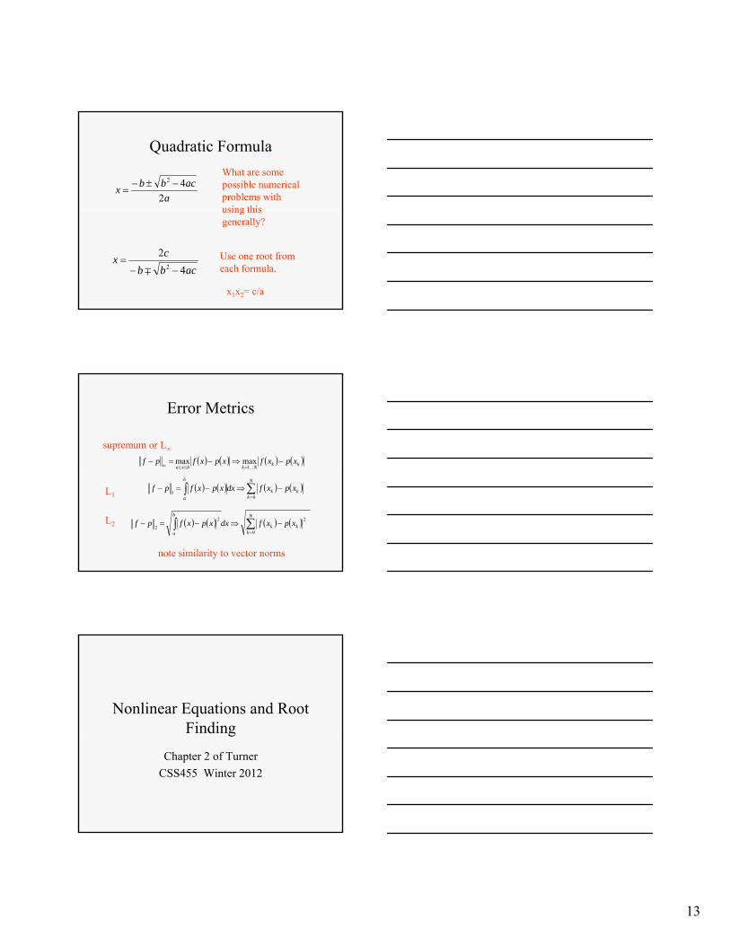
Quadratic Formula

aacbbx

242 −±−

=

What are some possible numerical problems with using thisusing this generally?

acbbcx

42

2 −−=

∓Use one root from each formula.

x1x2= c/a

Error Metrics

supremum or L∞

( ) ( ) ( ) ( )kkNkbxaxpxfxpxfpf −⇒−=−

=≤≤∞ ...1maxmax

L1( ) ( ) ( ) ( )∑∫

=

−⇒−=−N

kkk

b

a

xpxfdxxpxfpf0

1

L2 ( ) ( ) ( ) ( )∑∫=

−⇒−=−N

kkk

b

a

xpxfdxxpxfpf0

22

2

note similarity to vector norms

Nonlinear Equations and Root Findingg

Chapter 2 of TurnerCSS455 Winter 2012

14

How would you find?

• A solution to the equation

)(*1012 )cos(*102 xx

x =−

•Discuss with partner

•see demo testfn.m

Plot it first!

• Trial Equationf(x) = x2 – (1/x) -10*cos(x) =0

• Plot f(x) to learn of its• Plot f(x) to learn of its general behavior.

Plot it first!

• Another Trial Equationxsin(x) = 1 0

5

10

• orf(x) = xsin(x) - 1 =0

• Plot f(x) to learn of its general behavior.

-15 -10 -5 0 5 10 15-15

-10

-5

15

-0.2

0

0.2

0.4

0.6

0.8

1

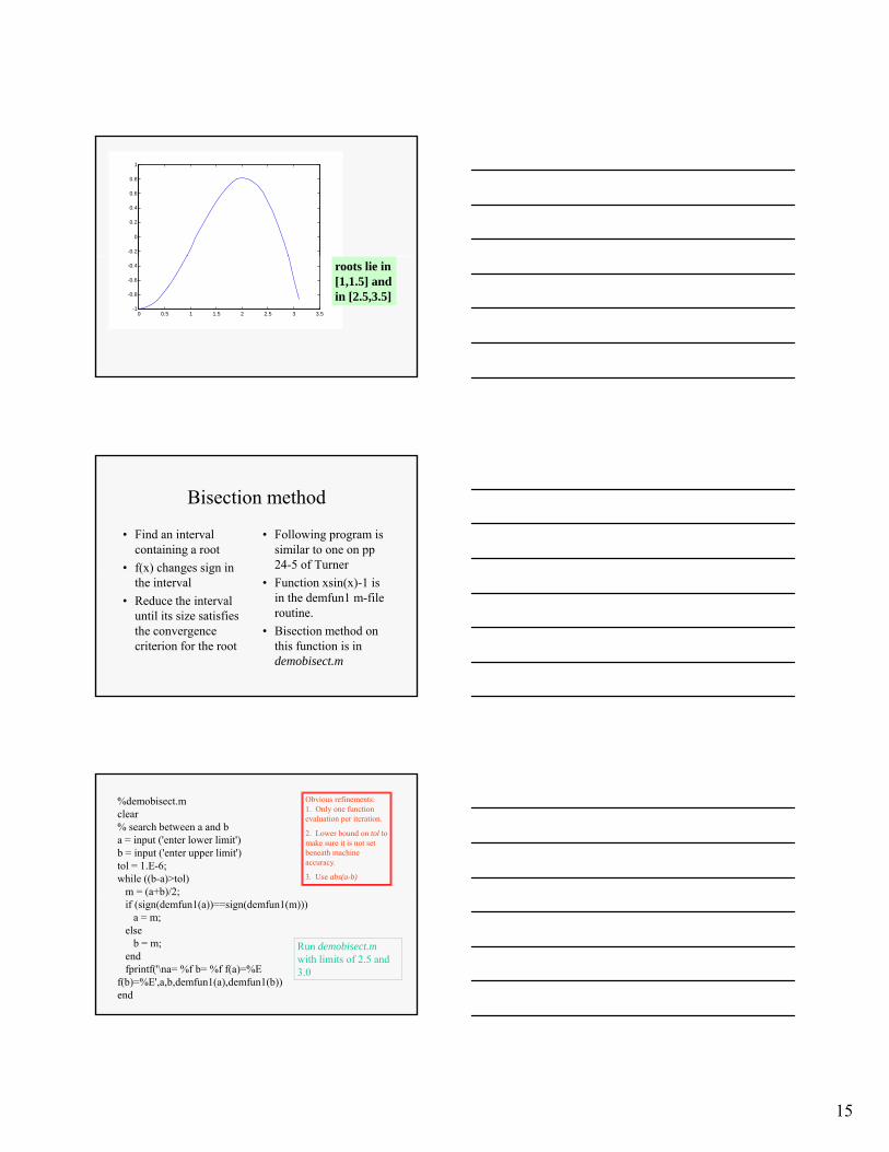
0 0.5 1 1.5 2 2.5 3 3.5-1

-0.8

-0.6

-0.4 roots lie in [1,1.5] and in [2.5,3.5]

Bisection method

• Find an interval containing a root

• f(x) changes sign in

• Following program is similar to one on pp 24-5 of Turner

the interval• Reduce the interval

until its size satisfies the convergence criterion for the root

• Function xsin(x)-1 is in the demfun1 m-file routine.

• Bisection method on this function is in demobisect.m

%demobisect.mclear% search between a and ba = input ('enter lower limit')b = input ('enter upper limit')tol = 1.E-6;while ((b-a)>tol)

m = (a+b)/2;

Obvious refinements:1. Only one function evaluation per iteration.

2. Lower bound on tol to make sure it is not set beneath machine accuracy.

3. Use abs(a-b)

m (a b)/2;if (sign(demfun1(a))==sign(demfun1(m)))

a = m;else

b = m;endfprintf('\na= %f b= %f f(a)=%E

f(b)=%E',a,b,demfun1(a),demfun1(b))end

Run demobisect.mwith limits of 2.5 and 3.0

16

a= 2.500000 b= 3.000000 f(a)=4.961804E-001 f(b)=-5.766400E-001a= 2.750000 b= 3.000000 f(a)=4.956773E-002 f(b)=-5.766400E-001a= 2.750000 b= 2.875000 f(a)=4.956773E-002 f(b)=-2.425928E-001a= 2.750000 b= 2.812500 f(a)=4.956773E-002 f(b)=-9.104357E-002a= 2.750000 b= 2.781250 f(a)=4.956773E-002 f(b)=-1.934543E-002a= 2.765625 b= 2.781250 f(a)=1.546218E-002 f(b)=-1.934543E-002a= 2.765625 b= 2.773438 f(a)=1.546218E-002 f(b)=-1.854219E-003a= 2.769531 b= 2.773438 f(a)=6.825878E-003 f(b)=-1.854219E-003a= 2 771484 b= 2 773438 f(a)=2 491298E 003 f(b)= 1 854219E 003a= 2.771484 b= 2.773438 f(a)=2.491298E-003 f(b)=-1.854219E-003a= 2.772461 b= 2.773438 f(a)=3.199059E-004 f(b)=-1.854219E-003a= 2.772461 b= 2.772949 f(a)=3.199059E-004 f(b)=-7.668150E-004a= 2.772461 b= 2.772705 f(a)=3.199059E-004 f(b)=-2.233692E-004a= 2.772583 b= 2.772705 f(a)=4.828971E-005 f(b)=-2.233692E-004

a= 2.772583 b= 2.772644 f(a)=4.828971E-005 f(b)=-8.753439E-005a= 2.772583 b= 2.772614 f(a)=4.828971E-005 f(b)=-1.962101E-005a= 2.772598 b= 2.772614 f(a)=1.433469E-005 f(b)=-1.962101E-005a= 2.772598 b= 2.772606 f(a)=1.433469E-005 f(b)=-2.643078E-006a= 2.772602 b= 2.772606 f(a)=5.845825E-006 f(b)=-2.643078E-006a= 2.772604 b= 2.772606 f(a)=1.601379E-006 f(b)=-2.643078E-006a= 2.772604 b= 2.772605 f(a)=1.601379E-006 f(b)=-5.208484E-007»

•This process is linearly convergent. It takes the same number of iterations to add n bits of precision regardless of the position within the sequence. Why?

•Requires only the value of the function

•Does not make use of magnitudes.

3x3 - 5x2 - 4x +4 = 0

• Apply bisection method in [0,1] (#1, p 27)• Plot it first! (plotfn.m)• Use demobisect2 to solve• Use demobisect2 to solve.

17

Newton’s Method•Can we use the knowledge of the slope at xc to help find the root?

Root at f(x) = 0

Newton’s Method•The slope of the straight line is given by the derivative of f(x) at xc •f(x+) = f(xc) + f ′(xc) [x+-xc] c c corx+ = xc + [f(x+)- f(xc)] / f ′(xc)

Root at f(x) = 0

Newton’s Method•Alternatively, view as a Taylor’s expansion about xc

...)()()()()()(2

c xfxxxfxxxfxf +′′−+′−+= +

)()()(

)()(

)()()()()()(

...)(2

)()()()(

c

cc

cc

c

ccc

cccc

xfxfxfxx

xxxf

xfxfxfxxxfxf

xfxfxxxfxf

′−

+=

−≈′−

′−+≈

+++

++

++

++

++

18

Newton’s Methodf(x+)=0 at a rootx+ = xc - f(xc) / f ′(xc)In our case f(x) = x sin(x) -1f ′(x) = sin(x) + xcos(x)

Newton’s Method

• Start at x = 3.5• Converges in only

Iterant: xn+1 = xn - f(xn) / f ′(xn)

five iterations• quadratic

convergence:# of digits is doubled at each iteration.

xcurr= 2.886023 xprev = 3.500000xcurr= 2.779536 xprev = 2.886023xcurr= 2.772635 xprev = 2.779536xcurr= 2.772605 xprev = 2.772635xcurr= 2.772605 xprev = 2.772605»

Newton’s Method

• Starting at x = 2.6, it converges to the same root

xcurr =2.6000

xcurr= 2.798728 xprev = 2.600000xcurr= 2.773026 xprev = 2.798728xcurr= 2.772605 xprev = 2.773026

• starting at x = 2 it converges to a very different root

xcurr 2.772605 xprev 2.773026xcurr= 2.772605 xprev = 2.772605»

xcurr= -8.630584 xprev = 2.000000xcurr= -9.596971 xprev = -8.630584xcurr= -9.322270 xprev = -9.596971xcurr= -9.317247 xprev = -9.322270xcurr= -9.317243 xprev = -9.317247xcurr= -9.317243 xprev = -9.317243»

19

Newton’s Method

• starting at x = 1.11, it converges to the nearby root.

•Convergence:Quadratic, but not guaranteed.

•Requires derivative.

• xcurr =• 1.1100• xcurr= 1.114156 xprev = 1.110000• xcurr= 1.114157 xprev = 1.114156»

3x3 - 5x2 - 4x +4 = 0

• Apply Newton method near x = 0.7 (#1 on p. 41). All you need is the function (above) and the derivative. demonewton2.m

Systems of Nonlinear Equations

20

systems of nonlinear equations

• Consider Example 12 on p. 46– Two equations - two unknowns– Behavior depends strongly on exact detail ofBehavior depends strongly on exact detail of

the equations• Apply some of the same methods applied to

the scalar nonlinear case:– e.g. Newton’s method

Make plausible

• System of two equations (f,g) in two variables (x,y) similar to that of previous examplep

• Two Equations in two unknowns:

01),(044),(

32

21212

22

21211

=−==−+=

xxxxfxxxxf

)( 21212f

In vector notation: f(x) =0

21

Newton’s Method• As in the scalar case, convergence will be

faster if it is started close to root.• In the scalar case, the derivative of the

function as well as the function itself wasfunction as well as the function itself was required at each iteration.

• In the multidimensional case, the Jacobian of the function plays this role. (nontrivial evaluation.)

write in vector notation• x is the vector of x1 and x2

• f is the vector of f1 and f2 evaluated with x• Jf is the Jacobian of f

⎤⎡ 22 44

⎟⎟⎠

⎞⎜⎜⎝

⎛=

=⎥⎦

⎤⎢⎣

⎡

−−+

=

2

1

32

21

22

21 0

144

)(

xx

xxxx

x

xf

Partial derivatives:differentiate the function fwith respect to one of its variables, treating the others as if they were constants.

J is a square matrix, each element of which is a partial derivative of one of the equations in the set.

22

11

22

2121

2

8

044),(

xxf

xxf

xxxxf

=⎟⎠⎞⎜

⎝⎛

∂∂

=⎟⎠⎞⎜

⎝⎛

∂∂

=−+=

22

⎟⎟⎠

⎞⎜⎜⎝

⎛=

⎟⎟⎟⎞

⎜⎜⎜⎛

∂∂∂

∂∂

∂

=

∂∂

=

22

21

321

21

22

2

1

1

1

3228

)()(

xxxxxx

ffx

fx

fx

f

j

i

J

xxJ ij

⎠⎝⎟⎠

⎜⎝ ∂∂ 2121

2

2

1

2 32 xxxxx

fx

f

xk+1 = xk - J-1f(compare to scalar case)

xn+1 = xn - f(xn) / f ′(xn)

What is the definition of a matrix inverse?

• In practice, we would avoid the inversion of J. But, here it will be done.

• The equations are written out explicitly on p.45-46 for the 2x2 case. You need now!

• The iterative formula then becomese e ve o u e beco esxk+1 = xk + sk, with

• sk= - J-1f• the two components of s are given by h and

k in text) See demosysnewton.m

⎟⎟⎠

⎞⎜⎜⎝

⎛=

kh

s

2 x 2 system by Newtonenter x .4enter y 1.8

4.000000000000000e-001 1.800000000000000e+000

4.045808966861598e-001 1.829261425167858e+000

4 041495644206274 001 1 829386038547648 +000

(x,y) (x1, x2)

Check4.041495644206274e-001 1.829386038547648e+000

4.041494570206883e-001 1.829385925812154e+000

4.041494570206443e-001 1.829385925812177e+000

EDU>>

Check convergence

23

Activity 3

Fixed Point Iteration (Activity)• Solve the equation to yield the form

x = g(x)• x[n+1] = g(x[n]) (start with guess and iterate)• F(x) = xsin(x) -1 =0 can be solved to yield:• F(x) = xsin(x) -1 =0, can be solved to yield:• x[n+1] = 1/sin(x[n]), and iterate starting from initial

guess x[0]

• Convergence depends upon nature of curve in vicinity of root.

• Will not converge to root near x = 2.77|g’(x)| > 1 (see demoiter.m)

x1= 7.086167 x0= 3.000000 x1= 1.389988 x0= 7.086167 x1= 1.016571 x0= 1.389988 x1= 1.176044 x0= 1.016571 x1= 1.083316 x0= 1.176044 x1= 1.131842 x0= 1.083316 x1= 1.104733 x0= 1.131842 x1= 1.119390 x0= 1.104733

x1= 1.114199 x0= 1.114081 x1= 1.114134 x0= 1.114199 x1= 1.114170 x0= 1.114134 x1= 1.114150 x0= 1.114170 x1= 1.114161 x0= 1.114150 x1= 1.114155 x0= 1.114161 x1= 1.114158 x0= 1.114155 x1= 1 114157 x0= 1 114158

x1= 1.111316 x0= 1.119390 x1= 1.115719 x0= 1.111316 x1= 1.113304 x0= 1.115719 x1= 1.114625 x0= 1.113304 x1= 1.113901 x0= 1.114625 x1= 1.114297 x0= 1.113901

x1= 1.114081 x0= 1.114297

x1= 1.114157 x0= 1.114158

x1= 1.114157 x0= 1.114157

24

• In this case, the algorithm converges to the root near x = 1.114, where |g’(x)| < 1

• Linearly convergent in this case.• Convergence depends strongly on form of iterant, which is

not unique.

02)( 2 =−−= xxxf

122)(

212)(2)(

)(

2

2

−+

==

+=+==−==

xxxgx

xxxxgx

xxgxf

The first one diverges for most starting guesses.

The other three converge at greatly differing rates.

3x3 - 5x2 - 4x +4 = 0

Apply fixed point iteration starting withx0 = 0.7 Use the two iterants on p. 34.

4531

34

34

35

23

2

xxx

xxx

−+=

−+= Finds root = 2

Finds root = 2/3

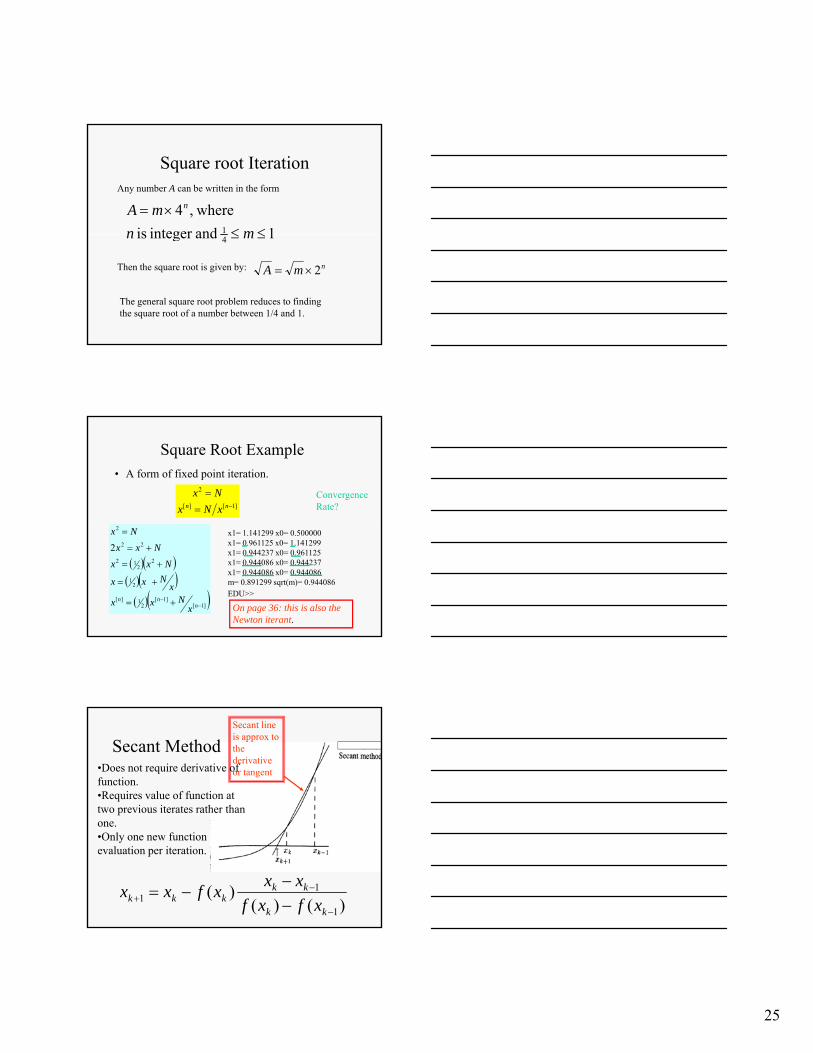
Square Root Example • A form of fixed point iteration.

]1[][

2

−==

nn xNxNx

2

( )( )( )( )( )( )]1[

]1[2

1][

21

22

12

22

2

2

−− +=

+=

+=

+=

=

nnn

xNxx

xNxx

NxxNxx

Nx The last iterant in the blue box is used after the procedure is scaled to require the square root of a number between 0.25 and 1.

25

Square root IterationAny number A can be written in the form

1andintegeris where,4

1 ≤≤×=

mnmA n

1 andinteger is 4 ≤≤ mn

Then the square root is given by: nmA 2×=

The general square root problem reduces to finding the square root of a number between 1/4 and 1.

Square Root Example • A form of fixed point iteration.

]1[][

2

−==

nn xNxNx

2

Convergence Rate?

( )( )( )( )( )( )]1[

]1[2

1][

21

22

12

22

2

2

−− +=

+=

+=

+=

=

nnn

xNxx

xNxx

NxxNxx

Nx x1= 1.141299 x0= 0.500000 x1= 0.961125 x0= 1.141299 x1= 0.944237 x0= 0.961125 x1= 0.944086 x0= 0.944237 x1= 0.944086 x0= 0.944086 m= 0.891299 sqrt(m)= 0.944086 EDU>>

On page 36: this is also the Newton iterant.

Secant MethodSecant line is approx to the derivative or tangent•Does not require derivative of

function.•Requires value of function at two previous iterates rather than

)()()(

1

11

−

−+ −

−−=

kk

kkkkk xfxf

xxxfxx

one. •Only one new function evaluation per iteration.

26

xk=2.5fxk = demfun1(xk);xkp1=4while (abs(xkp1-xk)>tol)

xkm1=xk;fxkm1=fxk;xk=xkp1;fxk=demfun1(xk);xkp1=xk-fxk*(xk-xkm1)/(fxk-fxkm1);fprintf('\nxkp1= %f xk = %f',xkp1,xk)

end

•Only one function evaluation per iteration.

Secant Methodf(x) = x sin(x) -1

• Starting at points x = 2.5 and 3.5, converges in 6 iterations.

xkp1= 2.682157 xk = 3.500000xkp1= 2.746235 xk = 2.682157xkp1= 2.774299 xk = 2.746235xkp1= 2.772575 xk = 2.774299

• convergence is still somewhat superlinear, although slower than Newton’s method

xkp1= 2.772605 xk = 2.772575xkp1= 2.772605 xk = 2.772605

Secant Method

• Starting at points x = 1.0 and 2.0 , converges in 4 i i

xkp1= 1.162240 xk = 1.000000xkp1= 1.114254 xk = 1.162240xkp1= 1.114157 xk = 1.114254xkp1= 1.114157 xk = 1.114157

iterations.• convergence is still

somewhat superlinear, although slower than Newton’s method

27

3x3 - 5x2 - 4x +4 = 0

Apply Secant method near x = 0.7 (#1 on p. 44)

Matlab fzero function.• fzero utilizes a hybrid method, starting with

bisection, switching to secant and to parabolic interpolation as appropriate.

• options = optimset('Display','iter','TolX',tol)

z = fzero(@demfun1,x,options)– x scalar: searches for root near initial x– x vector: guarantees a root between x(1) and x(2) if

funname has different signs at the two x-values.– TolX regulates convergence criterion– “iter” produces diagnostic output

fzero Output

28

Matrix Computations

CSS455 Winter 2011

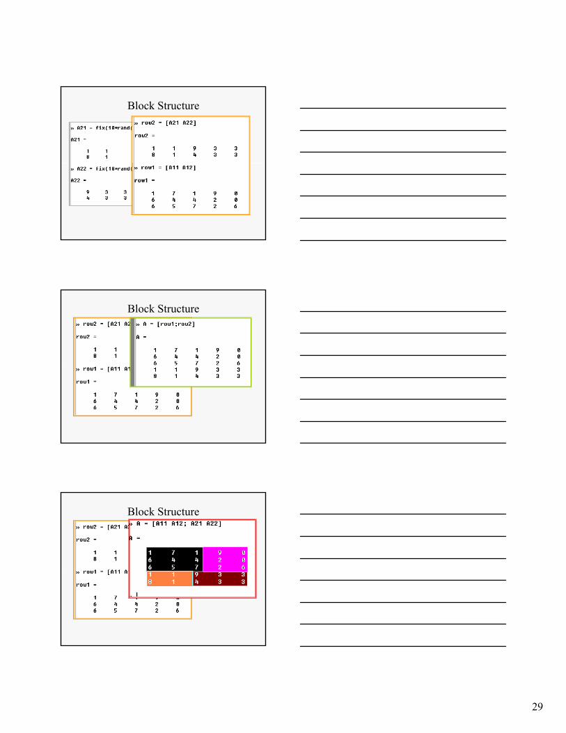
Block Structure of Matrices

• Overall matrix can be viewed as constructed of rows and columns of smaller matrices or blocks.

• Care must be taken to preserve correct dimensions.

• Matlab will generally check dimensions

Block Structure

29

Block Structure

Block Structure

Block Structure

30

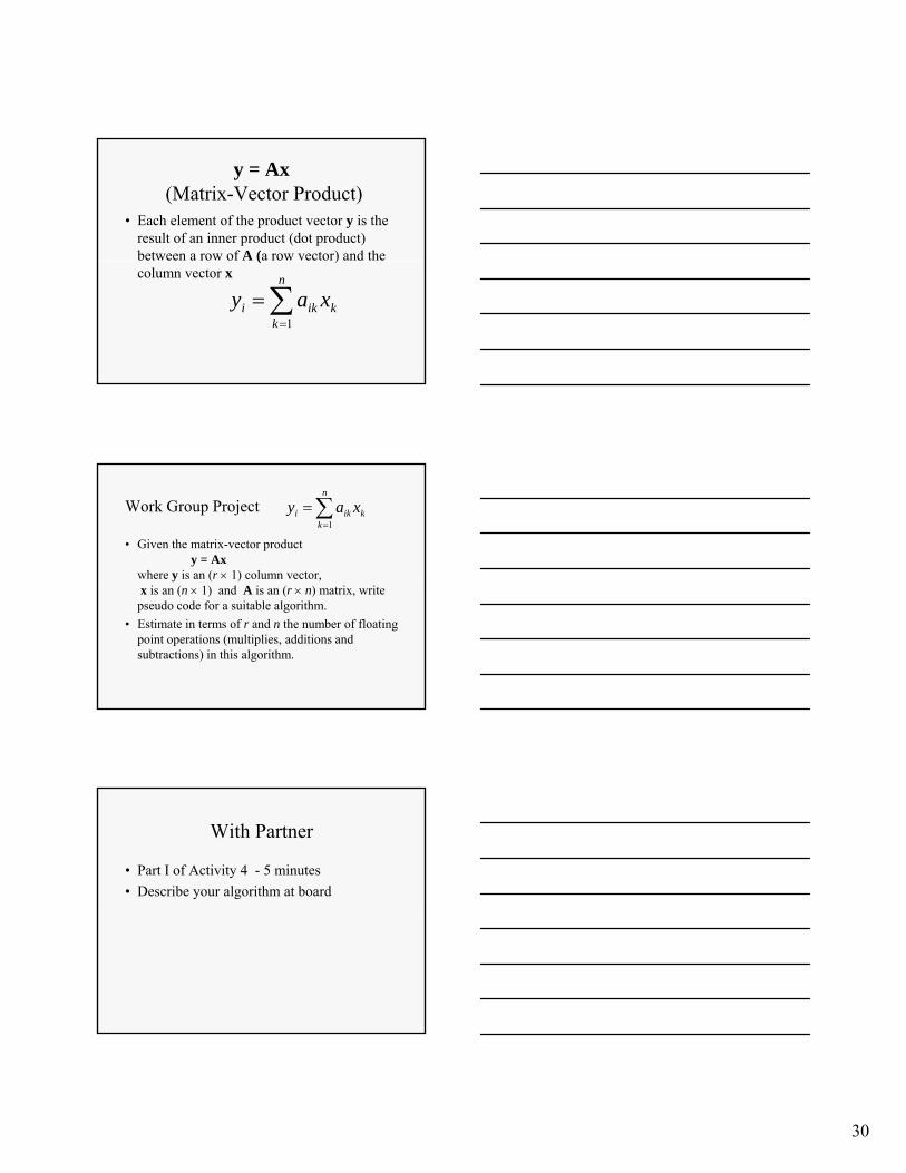
y = Ax(Matrix-Vector Product)

• Each element of the product vector y is the result of an inner product (dot product) between a row of A (a row vector) and the ( )column vector x

k

n

kiki xay ∑

=

=1

Work Group Project

• Given the matrix-vector producty = Ax

where y is an (r × 1) column vector, i ( 1) d A i ( ) i i

k

n

kiki xay ∑

=

=1

x is an (n × 1) and A is an (r × n) matrix, write pseudo code for a suitable algorithm.

• Estimate in terms of r and n the number of floating point operations (multiplies, additions and subtractions) in this algorithm.

With Partner

• Part I of Activity 4 - 5 minutes• Describe your algorithm at board

31

The element y1 is formed by the scalar product of row-1 of A with column x.

A y=Ax

x

r x n

n x 1

r x 1

∑=

=+++=n

iii

11n1n2121111 xaxaxaxay …

Ay=Ax

The element y2 is formed by the scalar product of row-2 of A with column x.

x

∑=

=+++=n

iii

12n2n2221212 xaxaxaxay …

y=Ax

r x n

n x 1

r x 1

Consider the elements of y

nn

xaxaxaxaxaxa

++++ 1212111

⎟⎟⎞

⎜⎜⎛

yy1

nmnmm

nn

xaxaxa

xaxaxa

++

++

2211

2222121

...⎟⎟⎟⎟

⎠⎜⎜⎜⎜

⎝

=

my

y2

32

Consider the elements of y

xaxaxa ++++ n1n212111 xaxaxa

⎟⎟⎞

⎜⎜⎛

yy1

nmnmm

nn

xaxaxa

xaxaxa

++

++

2211

2222121

...⎟⎟⎟⎟

⎠⎜⎜⎜⎜

⎝

=

my

y2

Row Ordered Algorithm%compute the Ax producty = zeros(m,1);for i = 1:m

y(i) = 0;for j = 1:nj

y(i) = y(i) + A(i,j)*x(j);end

end%Repeat with vector notationy2 = zeros(m,1);for i =1:m

y2(i) = A(i,:)*x;end

Matlab uses inner product in last loop.

Consider the elements of y

nn

xaxaxaxaxaxa

++++ 1212111

⎟⎟⎞

⎜⎜⎛

yy1

nmnmm

nn

xaxaxa

xaxaxa

++

++

2211

2222121

...⎟⎟⎟⎟

⎠⎜⎜⎜⎜

⎝

=

my

y2

33

Consider the elements of y

nn

xaxaxaxa

++++ 12121

2

11

xaxa Notice that there

is a natural column oriented

nmnm

nn

xaxa

xaxa

++

++

22

22221

...

1m1

21

xa

xa structure as well as the row structure. The code could be organized by column.

Column Oriented Approach - reverse the loop structure

In the inner loop x(j) is essentially a scalar constant

This can be thought of as “scalar a times vector x plus vector y” or “axpy”. If in single precision, called “saxpy”.

who cares?

• In matlab, the compact notation makes this h i l h b i

%Repeat with matrix notationy3 = A*x;

choice less than obvious:• The results and the number of floating point

operations are the same in the column and row oriented approaches.

• How could the choice be important?

34

Order of Data Storage

• If matrix A is stored row-wise:

312222111211 aaaaaaa nn

•The dot product approach might be efficient.

•If the data is stored column-wise, the saxpy approach might be more efficient:

132221212111 aaaaaaa mm

With Partner

• Part II of Acivity 4• Go to board with it

Matrix vector product with upper triagular matrix

⎟⎟⎟⎟⎟⎟⎟⎞

⎜⎜⎜⎜⎜⎜⎜⎛

=

⎟⎟⎟⎟⎟⎟⎟⎞

⎜⎜⎜⎜⎜⎜⎜⎛

⎟⎟⎟⎟⎟⎟⎟⎞

⎜⎜⎜⎜⎜⎜⎜⎛

4

3

2

1

4

3

2

1

464544

36353433

2625242322

161514131211

0000000

000

yyyyy

xxxxx

aaaaaaaaaaaaaaaaaaaa

Row oriented (dot product)

⎟⎟⎟⎟⎟⎟⎟⎞

⎜⎜⎜⎜⎜⎜⎜⎛

=

⎟⎟⎟⎟⎟⎟⎟⎞

⎜⎜⎜⎜⎜⎜⎜⎛

⎟⎟⎟⎟⎟⎟⎟⎞

⎜⎜⎜⎜⎜⎜⎜⎛

4

3

2

1

4

3

2

1

464544

36353433

2625242322

161514131211

0000000

000

yyyyy

xxxxx

aaaaaaaaaaaaaaaaaaaa

n

⎟⎟⎠

⎜⎜⎝

⎟⎟⎠

⎜⎜⎝⎟⎟⎠

⎜⎜⎝ 6

5

6

5

66

5655

000000000

yy

xx

aaa

a(j,j:n)*x(j:n) for each j (where * is dot product in Matlab)

⎟⎟⎠

⎜⎜⎝

⎟⎟⎠

⎜⎜⎝⎟⎟⎠

⎜⎜⎝ 6

5

6

5

66

5655

000000000

yy

xx

aaa

nnnn

n

jiijinjnjjjjjjj

n

iiinn

n

iiinn

xay

xaxaxaxay

xaxaxaxay

xaxaxaxay

=

=+++=

=+++=

=+++=

∑

∑

∑

=++

=

=

...

...

...

11,

2223232222

1112121111

35

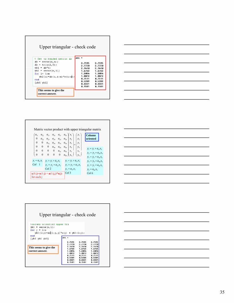
Upper triangular - check code

This seems to give the correct answer.

Matrix vector product with upper triangular matrix

⎟⎟⎟⎟⎟⎟⎟⎞

⎜⎜⎜⎜⎜⎜⎜⎛

=

⎟⎟⎟⎟⎟⎟⎟⎞

⎜⎜⎜⎜⎜⎜⎜⎛

⎟⎟⎟⎟⎟⎟⎟⎞

⎜⎜⎜⎜⎜⎜⎜⎛

5

4

3

2

1

5

4

3

2

1

5655

464544

36353433

2625242322

161514131211

0000000

000

yyyyy

xxxxx

aaaaaaaaaaaaaaaaaaaa

61611 xayy +=

Column oriented

⎟⎟⎠

⎜⎜⎝

⎟⎟⎠

⎜⎜⎝⎟⎟⎠

⎜⎜⎝ 6

5

6

5

66

5655

000000000

yy

xx

aaa

11111

Colxay =

222222

21211

Colxayy

xayy+=+=

33333

32322

31311

Colxay

xayyxayy

=+=+=

66666

65655

64644

63633

62622

Colxay

xayyxayyxayyxayy

=+=+=+=+=

y(1:j)=y(1:j) + a(1:j,j)*x(j)for each j

Upper triangular - check code

This seems to give the correct answer.

36

Matrix-Matrix products C= AB

• Each element of product is an inner (dot) product

∑=

=r

iijkikj BAC

1

between a row of A and one column vector.• Each column of the product is a matrix vector

product between A and one column of B.• The entire C matrix is just a collection of matrix-

vector products, and will have the same range of algorithms.

The element C21 is formed by the scalar product of row-2 of A with column-1 of B.

A B C=AB

∑=

=+++=r

iii

112n12n2122112121 babababac …

m x r

r x n

m x n

With Partner

• Activity 4, Part III• Results

37

Work Group Project

• Given the matrix-matrix productC=AB

where A is an (m × r) matrix, B is an (r × n) i d C i ( ) i i d

∑=

=r

iijkikj BAC

1

matrix and C is an (m × n) matrix write pseudo code for a suitable algorithm.

• Estimate in terms of m, n, and r the number of floating point operations (multiplies, additions and subtractions) in this algorithm.

C = AB in full triple loop notation

This is formally an n3 operation.

The inner loop is a vector inner product.

Run the inner loop like an inner vector product.

38

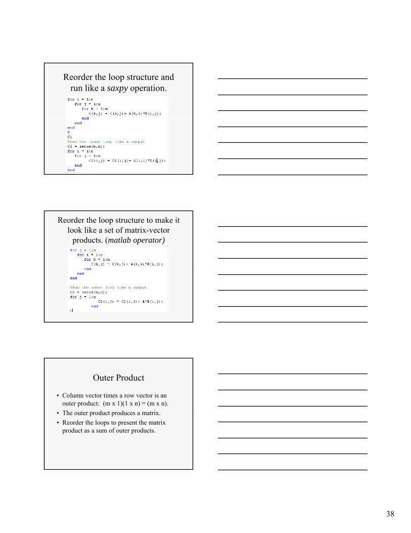
Reorder the loop structure and run like a saxpy operation.

Reorder the loop structure to make it look like a set of matrix-vector

products. (matlab operator)

Outer Product

• Column vector times a row vector is an outer product: (m x 1)(1 x n) = (m x n).

• The outer product produces a matrixThe outer product produces a matrix.• Reorder the loops to present the matrix

product as a sum of outer products.

39

Reorder loops

•k-loop looks like column vector times scalar (saxpy)

•jk loops look like column vector times a row vector (outer product)

•ijk loops look like sum of outer products, each of which is (m x n).

Outer Product Formulation

Windows Matlab timings(running MatBench from text)n Dot Saxpy MatVec Outer Direct

------------------------------------------------10 0.0180 0.0003 0.0003 0.0022 0.0001 50 0.0056 0.0022 0.0002 0.0008 0.0001 100 0.0237 0.0103 0.0012 0.0052 0.0005 200 0.1166 0.0557 0.0066 0.0369 0.0039 400 0.8740 0.3439 0.0896 1.2878 0.0320 800 8.0158 2.5688 1.1946 12.6034 0.2466 >>

MatVec and Direct clearly fastest for all lengths. Both of them use matlab operator for most time consuming steps.

These are elapsed times are from tic/toc in wall-clock seconds.

>>

40

Linux Matlab (#17)(running MatBench from text)n Dot Saxpy MatVec Outer Direct

------------------------------------------------10 0.0342 0.0020 0.0026 0.0017 0.0000 50 0.0123 0.0047 0.0004 0.0012 0.0005 100 0.0553 0.0219 0.0019 0.0156 0.0003 200 0.2563 0.1084 0.0134 0.1606 0.0050 400 1.4821 0.7356 0.2074 0.9561 0.0157 800 13 4897 4 9986 1 7941 7 3177 0 1123

Some times are slower, others are faster..

These are elapsed times in seconds.

800 13.4897 4.9986 1.7941 7.3177 0.1123 >>

Comparisonn Dot Saxpy MatVec Outer Direct

------------------------------------------------10 0.0180 0.0003 0.0003 0.0022 0.0001 50 0.0056 0.0022 0.0002 0.0008 0.0001 100 0.0237 0.0103 0.0012 0.0052 0.0005 200 0.1166 0.0557 0.0066 0.0369 0.0039 400 0.8740 0.3439 0.0896 1.2878 0.0320

n Dot Saxpy MatVec Outer Direct------------------------------------------------10 0.0180 0.0003 0.0003 0.0022 0.0001 50 0.0056 0.0022 0.0002 0.0008 0.0001 100 0.0237 0.0103 0.0012 0.0052 0.0005 200 0.1166 0.0557 0.0066 0.0369 0.0039 400 0.8740 0.3439 0.0896 1.2878 0.0320 800 8 0158 2 5688 1 1946 12 6034 0 2466800 8.0158 2.5688 1.1946 12.6034 0.2466 >>800 8.0158 2.5688 1.1946 12.6034 0.2466 >> n Dot Saxpy MatVec Outer Direct

------------------------------------------------10 0.0342 0.0020 0.0026 0.0017 0.0000 50 0.0123 0.0047 0.0004 0.0012 0.0005 100 0.0553 0.0219 0.0019 0.0156 0.0003 200 0.2563 0.1084 0.0134 0.1606 0.0050 400 1.4821 0.7356 0.2074 0.9561 0.0157 800 13.4897 4.9986 1.7941 7.3177 0.1123 >>

Activity 4 – Part IV