Accuracy on the Time-of-Flight Estimation for Ultrasonic

HAL Id: hal-01769820https://hal.archives-ouvertes.fr/hal-01769820

Preprint submitted on 18 Apr 2018

HAL is a multi-disciplinary open accessarchive for the deposit and dissemination of sci-entific research documents, whether they are pub-lished or not. The documents may come fromteaching and research institutions in France orabroad, or from public or private research centers.

L’archive ouverte pluridisciplinaire HAL, estdestinée au dépôt et à la diffusion de documentsscientifiques de niveau recherche, publiés ou non,émanant des établissements d’enseignement et derecherche français ou étrangers, des laboratoirespublics ou privés.

Accuracy on the Time-of-Flight Estimation forUltrasonic Waves Applied to Non-DestructiveEvaluation of Standing Trees: A Comparative

Experimental StudyLuis Espinosa, Jan Bacca, Flavio Prieto, Philippe Lasaygues, Loïc Brancheriau

To cite this version:Luis Espinosa, Jan Bacca, Flavio Prieto, Philippe Lasaygues, Loïc Brancheriau. Accuracy on theTime-of-Flight Estimation for Ultrasonic Waves Applied to Non-Destructive Evaluation of StandingTrees: A Comparative Experimental Study. 2018. �hal-01769820�

https://hal.archives-ouvertes.fr/hal-01769820

https://hal.archives-ouvertes.fr

Accuracy on the Time-of-Flight Estimation for Ultrasonic Waves

Applied to Non-Destructive Evaluation of Standing Trees: A

Comparative Experimental Study

Luis Espinosa1,2), Jan Bacca3), Flavio Prieto1), Philippe Lasaygues4), Loıc Brancheriau2)

1) Dept. of Mechanical and Mechatronics Engineering, Universidad Nacional de ColombiaCarrera 45 No. 26-85, Bogota, Colombia. [email protected]

2) Research Unit BioWooEB, Univ Montpellier, CIRADTA B114/16, 73 Rue J.F. Breton, Montpellier, France

3) Dept. of Electrical and Electronics Engineering, Universidad Nacional de ColombiaCarrera 45 No. 26-85, Bogota, Colombia

4) Aix Marseille Univ, CNRS, Centrale Marseille, LMA, 4, Impasse Nikola TESLACS 40006, Marseille, France.

Summary1

Time-of-flight measurement is a critical step to per-2

form ultrasonic non-destructive testing of standing3

trees, with direct influence on the precision of de-4

fect detection. Aiming to increase the accuracy on5

the estimation, the characteristics of the ultrasonic6

measurement chain should be adapted to the con-7

straints of wood testing in living condition. This8

study focused on the excitation signal parameters,9

such as shape, temporal duration, and frequency re-10

sponse, and then the selection of a suitable time-11

of-flight determination technique. A standing plane12

tree was tested, placing ultrasonic receivers at four13

different positions, with five different excitation sig-14

nals and three time-of-flight detection methods. The15

proposed ultrasonic chain of measurement resulted in16

high signal-to-noise ratios in received signals for all17

configurations. A time-frequency analysis was used18

to determine the power distribution in the frequency19

domain, showing that only chirp signal could concen-20

trate the power around the resonant frequency of the21

sensor. Threshold and Akaike information criterion22

method performed similar for impulsive signals with23

decreasing uncertainty as sensor position approached24

to the radial direction. Those two methods failed to25

accurate determine time-of-flight for Gaussian pulse26

and chirp signals. Cross-correlation was only suitable27

for the chirp signal, presenting the lower uncertainty28

values among all configurations.29

1 Introduction30

Modern techniques can be used to minimize the risk31

associated with tree failure. Significant advances in32

this field include decay detection equipments, formu-33

las and guidelines for assessing hazardous trees [1, 2]. 34

Standing tree quality can be evaluated using differ- 35

ent techniques [3]. First, a visual inspection is priv- 36

ileged, but can be insufficient to detect inner decay. 37

The use of specialized tools include micro-drill resis- 38

tance measurements [4], a widely used technique con- 39

sisting on drilling through the tree trunk following 40

a straight path while measuring the penetration re- 41

sistance. Basically, defects such as decay and cracks 42

present a reduced resistance to the drill, a pattern 43

that can be detected. However, this technique is lim- 44

ited by the selected orientation, it is difficult to assure 45

going through the defect. 46

Other group of techniques uses stress waves tim- 47

ing to evaluate wood quality and trees inner state. 48

The basic consideration is that decay inside wood 49

will have an influence in the propagation of elastic 50

waves: at low velocity regions, such as decay, veloc- 51

ity decreases and signal attenuation increases [5]. For 52

standing trees testing, commercial approaches include 53

the IML Impulse Hammer, the Fakkop 2D Microsec- 54

ond Timer and the Sylvatest [6]. Wood mechanical 55

properties can be estimated using the measured ve- 56

locities, for example, using the Christoffel equation 57

[7, 8, 9]. Accuracy on the time-of-flight estimation is 58

crucial to perform a correct wood evaluation. Addi- 59

tionally, resonance-based methods present an alterna- 60

tive for velocity detection based on the analysis of the 61

stress waves natural frequencies, traveling through the 62

wood [10, 11]. 63

Considering 2D imaging, ultrasonic tomography is 64

one of the techniques used for non-destructive control 65

of standing trees [12, 13, 14, 15, 16, 17, 18]. This 66

method consists on cross-sectional imaging from the 67

tree trunk using either reflection or transmission wave 68

propagation data. Usually, the parameter used to 69

Espinosa et al., p. 2

build the image is the time-of-flight (TOF) taken by70

the ultrasonic wave from the transmitter to the mul-71

tiple receivers. Thus, TOF determination is a critical72

step to perform image reconstruction [19]; image qual-73

ity is highly dependent on the precision of the TOF74

measurement.75

Considering conventional ultrasonic testing, the ob-76

ject is excited with a pulse, and TOF measurement77

rely on the estimation of the signal instantaneous78

power by determining the first arrival above a noise79

threshold, defined by the user [20, 21]. Also, a pulse80

train can be used to boost the transmitted energy81

for a specific frequency [22]. Automatic methods for82

detecting first arrivals have been proposed, including83

pickers based on the Akaike information criteria (AIC)84

[23, 24] and the Hinkley criteria [25]. Alternatives in-85

clude the transmission of encoded waveforms, such86

as the chirp-coded excitation method, where a recog-87

nizable signature is sent through the media and the88

TOF is estimated using a cross-correlation function89

[26, 27, 28]. In consideration of the wide range of sig-90

nals and TOF detection techniques, the choice of pa-91

rameters for standing tree ultrasonic testing demands92

an evaluation of the accuracy of the aforementioned93

methods.94

This study aimed to compare several signal shapes95

and TOF detection methods, for setting up an ul-96

trasonic chain of measurement in order to perform97

non-destructive evaluation of standing trees. Impul-98

sive and encoded signals were tested, combined with99

three different methods for TOF estimation: Thresh-100

old, AIC method and cross-correlation. First, ex-101

perimental setting is presented, including electrical102

specification for the ultrasonic chain, the excitation103

signal parameters and a description of the TOF de-104

tection methods. Then, energy and signal-to-noise105

ratios are computed for all configurations. A time-106

frequency analysis using the Gabor transform is per-107

formed, aiming to inspect energy distribution. Lastly,108

wave transit times are reported, computing dispersion109

among experiments repetition, to establish which set-110

ting leads to highest accuracy.111

2 Materials and methods112

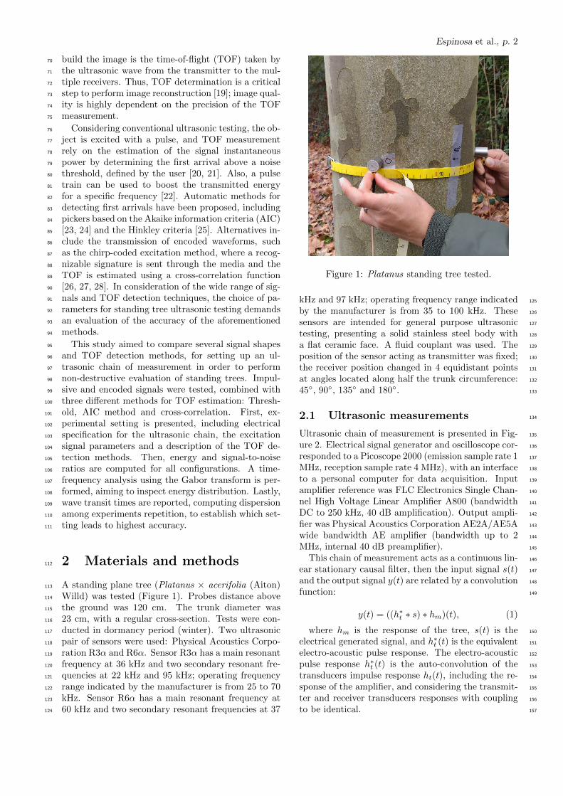
A standing plane tree (Platanus × acerifolia (Aiton)113

Willd) was tested (Figure 1). Probes distance above114

the ground was 120 cm. The trunk diameter was115

23 cm, with a regular cross-section. Tests were con-116

ducted in dormancy period (winter). Two ultrasonic117

pair of sensors were used: Physical Acoustics Corpo-118

ration R3α and R6α. Sensor R3α has a main resonant119

frequency at 36 kHz and two secondary resonant fre-120

quencies at 22 kHz and 95 kHz; operating frequency121

range indicated by the manufacturer is from 25 to 70122

kHz. Sensor R6α has a main resonant frequency at123

60 kHz and two secondary resonant frequencies at 37124

Figure 1: Platanus standing tree tested.

kHz and 97 kHz; operating frequency range indicated 125

by the manufacturer is from 35 to 100 kHz. These 126

sensors are intended for general purpose ultrasonic 127

testing, presenting a solid stainless steel body with 128

a flat ceramic face. A fluid couplant was used. The 129

position of the sensor acting as transmitter was fixed; 130

the receiver position changed in 4 equidistant points 131

at angles located along half the trunk circumference: 132

45◦, 90◦, 135◦ and 180◦. 133

2.1 Ultrasonic measurements 134

Ultrasonic chain of measurement is presented in Fig- 135

ure 2. Electrical signal generator and oscilloscope cor- 136

responded to a Picoscope 2000 (emission sample rate 1 137

MHz, reception sample rate 4 MHz), with an interface 138

to a personal computer for data acquisition. Input 139

amplifier reference was FLC Electronics Single Chan- 140

nel High Voltage Linear Amplifier A800 (bandwidth 141

DC to 250 kHz, 40 dB amplification). Output ampli- 142

fier was Physical Acoustics Corporation AE2A/AE5A 143

wide bandwidth AE amplifier (bandwidth up to 2 144

MHz, internal 40 dB preamplifier). 145

This chain of measurement acts as a continuous lin- 146

ear stationary causal filter, then the input signal s(t) 147

and the output signal y(t) are related by a convolution 148

function: 149

y(t) = ((h∗t ∗ s) ∗ hm)(t), (1)

where hm is the response of the tree, s(t) is the 150

electrical generated signal, and h∗t (t) is the equivalent 151

electro-acoustic pulse response. The electro-acoustic 152

pulse response h∗t (t) is the auto-convolution of the 153

transducers impulse response ht(t), including the re- 154

sponse of the amplifier, and considering the transmit- 155

ter and receiver transducers responses with coupling 156

to be identical. 157


Tree

Signal

generatorOscilloscope

Transmitter Receiver

40dB 40dB

0

4590

135

180o

o

oo

o

y(t)

hm(t)

s(t)

ht(t) ht(t)

Figure 2: Ultrasonic chain for measurements.

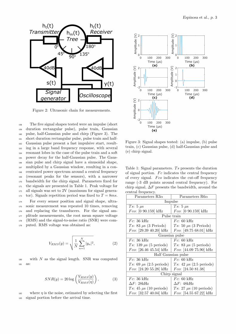
The five signal shapes tested were an impulse (short158

duration rectangular pulse), pulse train, Gaussian159

pulse, half-Gaussian pulse and chirp (Figure 3). The160

short duration rectangular pulse, pulse train and half-161

Gaussian pulse present a fast impulsive start, result-162

ing in a large band frequency response, with several163

resonant lobes in the case of the pulse train and a soft164

power decay for the half-Gaussian pulse. The Gaus-165

sian pulse and chirp signal have a sinusoidal shape,166

multiplied by a Gaussian window, resulting in a con-167

centrated power spectrum around a central frequency168

(resonant peaks for the sensors), with a narrower169

bandwidth for the chirp signal. Parameters fixed for170

the signals are presented in Table 1. Peak voltage for171

all signals was set to 2V (maximum for signal genera-172

tor). Signals repetition period was fixed to T = 8ms.173

For every sensor position and signal shape, ultra-174

sonic measurement was repeated 10 times, removing175

and replacing the transducers. For the signal am-176

plitude measurements, the root mean square voltage177

(RMS) and the signal-to-noise ratio (SNR) were com-178

puted. RMS voltage was obtained as:179

VRMS(y) =

√√√√ 1

N

N∑n=1

|yn|2, (2)

with N as the signal length. SNR was computed180

as:181

SNR(y) = 20 log

(VRMS(y)

VRMS(η)

), (3)

where η is the noise, estimated by selecting the first182

signal portion before the arrival time.183

0 100 200 300

Time (µs)

0

1

2

Am

plitu

de

(V)

(a)

0 100 200 300

Time (µs)

0

1

2

Am

plitu

de (

V)

(b)

0 100 200 300

Time (µs)

-2

0

2

Am

plitu

de (

V)

(c)

0 100 200 300

Time (µs)

-1

0

1

2

Am

plitu

de (

V)

(d)

0 100 200 300

Time (µs)

-2

0

2

Am

plitu

de (

V)

(e)

Figure 3: Signal shapes tested: (a) impulse, (b) pulsetrain, (c) Gaussian pulse, (d) half-Gaussian pulse and(e) chirp signal.

Table 1: Signal parameters. Ts presents the durationof signal portion. Fc indicates the central frequencyof every signal. Fco indicates the cut-off frequencyrange (-3 dB points around central frequency). Forchirp signal, ∆F presents the bandwidth, around thecentral frequency.

Parameters R3α Parameters R6αImpulse

Ts: 5 µs Ts: 5 µsFco: [0 90.159] kHz Fco: [0 90.159] kHz

Pulse trainFc: 36 kHz Fc: 60 kHzTs: 83 µs (3 Periods) Ts: 50 µs (3 Periods)Fco: [29.39 40.20] kHz Fco: [49.75 68.01] kHz

Gaussian pulseFc: 36 kHz Fc: 60 kHzTs: 139 µs (5 periods) Ts: 83 µs (5 periods)Fco: [26.46 45.54] kHz Fco: [44.09 75.90] kHz

Half Gaussian pulseFc: 36 kHz Fc: 60 kHzTs: 69 µs (2.5 periods) Ts: 42 µs (2.5 periods)Fco: [24.20 55.28] kHz Fco: [24.50 81.38]

Chirp signalFc: 36 kHz Fc: 60 kHz∆F : 28kHz ∆F : 48kHzTs: 45 µs (10 periods) Ts: 27 µs (10 periods)Fco: [32.57 40.04] kHz Fco: [54.55 67.22] kHz


2.2 Time-of-flight detection methods184

Threshold185

Threshold level for the received signal had to be de-186

fined above the noise level [16]. The threshold level is187

defined to be m times the standard deviation of the188

noise, with m as a user-defined parameter. For the ex-189

periments, this value was constant and fixed by trial190

and error to 8. TOF is then selected to be the first191

time point where signal is above the threshold level.192

AIC method193

This method assumes that signal can be divided into194

two local stationary segments, before and after the on-195

set time, each one modeled as an autoregressive pro-196

cess. The time instant where the Akaike information197

criterion (AIC) is minimized, corresponds to the op-198

timal separation between noise and signal, this is, the199

onset time [22]. For a signal divided at point k into200

two segments y1 (before k) and y2 (after k), the AIC201

criterion is computed as:202

AIC[k] = k log(σ2(y1)) + (N − k) log(σ2(y2)). (4)

TOF value is obtained by founding the time point203

where the AIC criterion reach the global minimum.204

Cross-correlation205

When a recognizable signature is sent through the206

media, such as chirp signal, input and output signals207

delay time can be obtained using cross-correlation208

[26, 27, 28]. The maximum value for the cross-209

correlation function between two signals indicates210

their delay time. Normalized cross-correlation func-211

tion is:212

rsy[l] =1√EsEy

N∑k=0

s[k]y[k − l], (5)

where Es and Ey correspond to the signals energy and213

N is the signal length.214

3 Results215

3.1 Signal amplitude measurement216

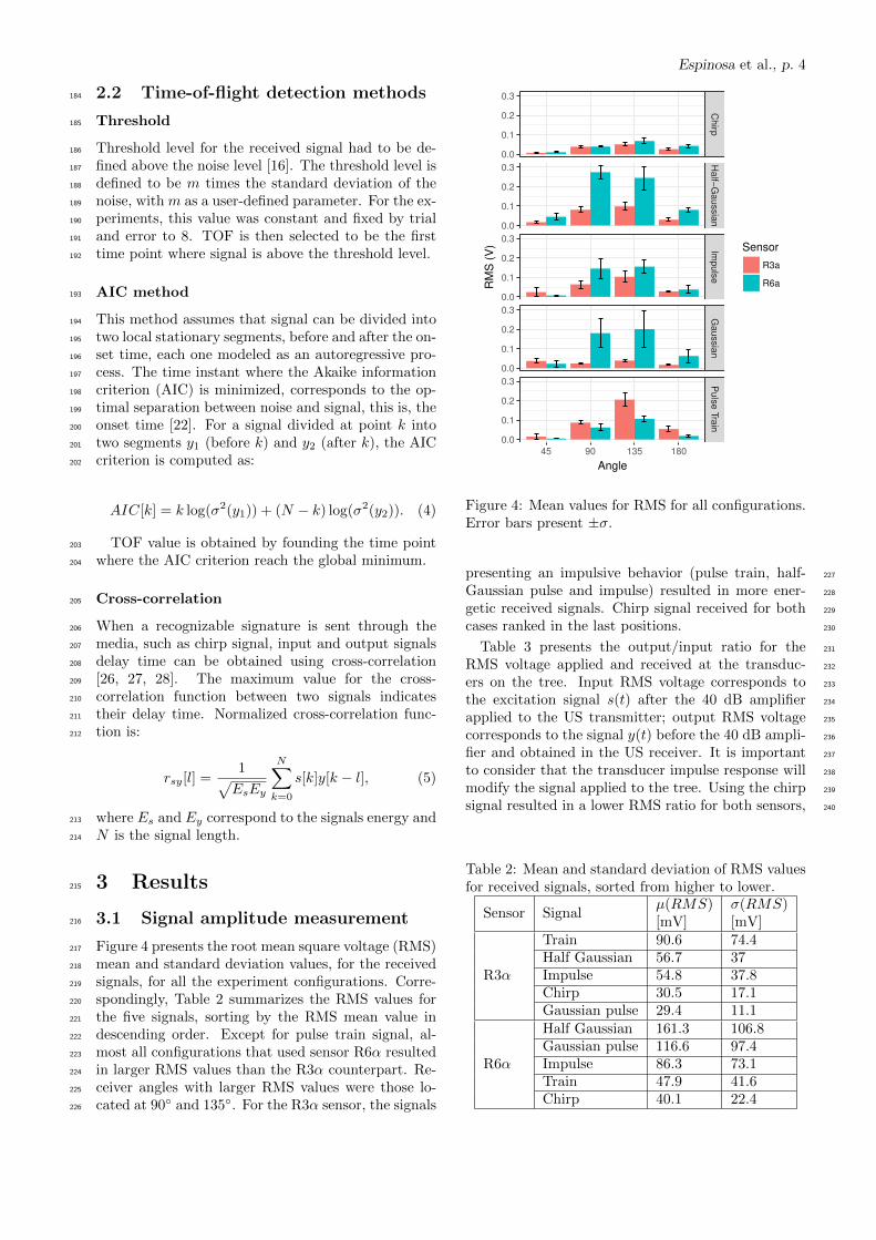
Figure 4 presents the root mean square voltage (RMS)217

mean and standard deviation values, for the received218

signals, for all the experiment configurations. Corre-219

spondingly, Table 2 summarizes the RMS values for220

the five signals, sorting by the RMS mean value in221

descending order. Except for pulse train signal, al-222

most all configurations that used sensor R6α resulted223

in larger RMS values than the R3α counterpart. Re-224

ceiver angles with larger RMS values were those lo-225

cated at 90◦ and 135◦. For the R3α sensor, the signals226

Ch

irpH

alf−

Ga

ussia

nIm

pu

lse

Ga

ussia

nP

uls

e T

rain

45 90 135 180

0.0

0.1

0.2

0.3

0.0

0.1

0.2

0.3

0.0

0.1

0.2

0.3

0.0

0.1

0.2

0.3

0.0

0.1

0.2

0.3

Angle

RM

S (

V) Sensor

R3a

R6a

Figure 4: Mean values for RMS for all configurations.Error bars present ±σ.

presenting an impulsive behavior (pulse train, half- 227

Gaussian pulse and impulse) resulted in more ener- 228

getic received signals. Chirp signal received for both 229

cases ranked in the last positions. 230

Table 3 presents the output/input ratio for the 231

RMS voltage applied and received at the transduc- 232

ers on the tree. Input RMS voltage corresponds to 233

the excitation signal s(t) after the 40 dB amplifier 234

applied to the US transmitter; output RMS voltage 235

corresponds to the signal y(t) before the 40 dB ampli- 236

fier and obtained in the US receiver. It is important 237

to consider that the transducer impulse response will 238

modify the signal applied to the tree. Using the chirp 239

signal resulted in a lower RMS ratio for both sensors, 240

Table 2: Mean and standard deviation of RMS valuesfor received signals, sorted from higher to lower.

Sensor Signalµ(RMS)[mV]

σ(RMS)[mV]

R3α

Train 90.6 74.4Half Gaussian 56.7 37Impulse 54.8 37.8Chirp 30.5 17.1Gaussian pulse 29.4 11.1

R6α

Half Gaussian 161.3 106.8Gaussian pulse 116.6 97.4Impulse 86.3 73.1Train 47.9 41.6Chirp 40.1 22.4


Table 3: Ratio between output (y(t) before 40dB am-plification) and input (s(t) after 40dB amplification)RMS values for all signals, sorted from higher to lower.

Sensor Signals(t)VRMS

[mV]

y(t)VRMS

[mV]

Out/InRatio[dB]

R3α

Impulse 50.0 54.8 -79.2Half-Gaussian 54.9 56.7 -79.7Train 139.6 90.6 -83.7Gaussian pulse 78.5 29.4 -88.6Chirp 141.9 30.5 -93.6

R6α

Half-Gaussian 45 161.3 -68.9Gaussian pulse 60.8 116.6 -74.3Impulse 50.0 86.3 -75.2Train 109.5 47.9 -87.1Chirp 109.4 40.1 -88.6

Table 4: Mean and standard deviation of SNR valuesfor received signals, sorted from higher to lower.

Sensor Signalµ(SNR)[dB]

σ(SNR)[dB]

R3α

Train 33.11 6.48Impulse 32.67 5.31Gaussian pulse 29.77 5.08Half-Gaussian 29 7.09Chirp 27.58 7.21

R6α

Train 41.71 10.85Impulse 40.52 12.35Gaussian pulse 35.02 11.75Half-Gaussian 30.51 6.9Chirp 21.81 6.53

and signals such as the half Gaussian pulse and the241

impulse resulted in the larger ratios.242

Figure 5 presents the signal-to-noise ratio (SNR)243

mean and standard deviation values. Table 4 sum-244

marizes the SNR values, sorting by SNR mean value245

in descending order. Average SNR values over all re-246

ceiver angles ranged between 20 and 40 dB, indicating247

low presence of noise. Only exception correspond to248

chirp signal when using the R6α located at 45◦, where249

mean SNR was around 10 dB. As obtained for the250

RMS measurements, SNR values for the sensor R6α251

were higher than those obtained for R3α. Impulsive-252

like signals, as the pulse train and impulse, presented253

the highest SNR ratios.254

3.2 Time-frequency analysis255

As the frequency contents of the received signals var-256

ied over the time, we used a time-frequency analysis257

to obtain a representation of the input and output258

signals behavior for the ultrasonic chain of measure-259

ment. From several alternatives to perfom the time-260

frequency analysis, the Gabor transform was used261

[29, 30].262

Ch

irpH

alf−

Ga

ussia

nIm

pu

lse

Ga

ussia

nP

uls

e T

rain

45 90 135 180

0

20

40

0

20

40

0

20

40

0

20

40

0

20

40

Angle

SN

R (

dB

) Sensor

R3a

R6a

Figure 5: Mean values for SNR for all configurations.Error bars present ±σ.

For this study, resolution in time was set to 0.1 ms 263

and resolution in frequency was set to 5 kHz. The 264

receiver angle selected for the analysis was 135◦, con- 265

sidering it presents the most energetic signals, with 266

higher SNR ratios. 267

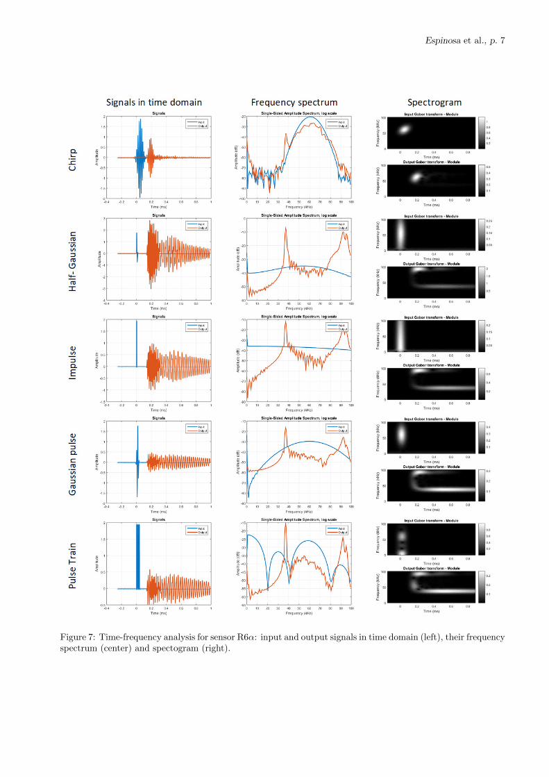
Figure 6 and Figure 7 present first the input and 268

output signals on time domain, then their frequency 269

spectrum and finally the input and output spectro- 270

grams, for sensors R3α and R6α respectively. 271

Chirp is the only signal able to concentrate the en- 272

ergy around the central frequency for both sensors on 273

the output signal. Gaussian pulse presented power 274

concentration at frequencies near to the excitation 275

central frequencies only for sensor R3α; mean power 276

frequencies did not correspond for sensor R6α where 277

energy dissipated at different frequencies from 60 kHz 278

(mainly 37 kHz and 97 kHz). The other signals pre- 279

sented energy concentration mainly on the other sen- 280

sor resonant peaks: for R3α at the third resonant 281

peak (95 kHz), and for R6α in first and third reso- 282

nant peaks (37 kHz and 97 kHz). 283

3.3 TOF determination 284

Time-of-flight was obtained for all the experiment 285

configurations, using the Threshold and AIC method. 286

Cross-correlation was used exclusively for the chirp 287

signal, given that is the only excitation signal with 288

a similar shape on the output for both sensors, and 289

therefore, chirp signal results are studied separately. 290

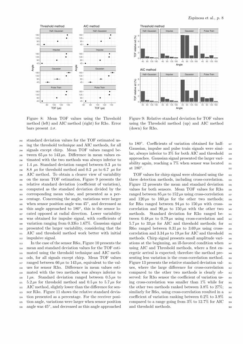
For the sensor R3α, Figure 8 shows the mean and 291


Figure 6: Time-frequency analysis for sensor R3α: input and output signals in time domain (left), frequencyspectrum (center) and spectogram (right).


Figure 7: Time-frequency analysis for sensor R6α: input and output signals in time domain (left), their frequencyspectrum (center) and spectogram (right).


Pulse Train

Gaussian

Impulse

Half−Gaussian

80 100 120 140

45

90

135

180

45

90

135

180

45

90

135

180

45

90

135

180

TOF (µs)

An

gle

Threshold method

Pulse Train

Gaussian

Impulse

Half−Gaussian

60 80 100 120 140

45

90

135

180

45

90

135

180

45

90

135

180

45

90

135

180

TOF (µs)

An

gle

AIC method

Figure 8: Mean TOF values using the Thresholdmethod (left) and AIC method (right) for R3α. Errorbars present ±σ.

standard deviation values for the TOF estimated us-292

ing the threshold technique and AIC methods, for all293

signals except chirp. Mean TOF values ranged be-294

tween 65µs to 143µs. Difference in mean values es-295

timated with the two methods was always inferior to296

1.4 µs. Standard deviation ranged between 0.3 µs to297

8.8 µs for threshold method and 0.2 µs to 6.7 µs for298

AIC method. To obtain a clearer view of variability299

on the mean TOF estimation, Figure 9 presents the300

relative standard deviation (coefficient of variation),301

computed as the standard deviation divided by the302

corresponding mean value, and presented as a per-303

centage. Concerning the angle, variations were larger304

when sensor position angle was 45◦, and decreased as305

this angle approached to 180◦, this is the sensor lo-306

cated opposed at radial direction. Lower variability307

was obtained for impulse signal, with coefficients of308

variation ranging from 0.33to 1.67%. Gaussian signal309

presented the larger variability, considering that the310

AIC and threshold method work better with initial311

impulsive signal.312

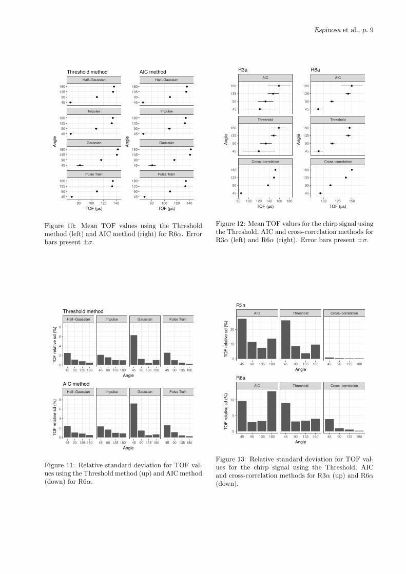
In the case of the sensor R6α, Figure 10 presents the313

mean and standard deviation values for the TOF esti-314

mated using the threshold technique and AIC meth-315

ods, for all signals except chirp. Mean TOF values316

ranged between 66µs to 143µs, equivalent to the val-317

ues for sensor R3α. Difference in mean values esti-318

mated with the two methods was always inferior to319

1µs. Standard deviation ranged between 0.5µs to320

5.2µs for threshold method and 0.5µs to 5.7µs for321

AIC method, slightly lower than the difference for sen-322

sor R3α. Figure 11 shows the relative standard devia-323

tion presented as a percentage. For the receiver posi-324

tion angle, variations were larger when sensor position325

angle was 45◦, and decreased as this angle approached326

Half−Gaussian Impulse Gaussian Pulse Train

45 90 135 180 45 90 135 180 45 90 135 180 45 90 135 180

0

2

4

6

8

Angle

TO

F r

ela

tive

sd

(%

)

Threshold method


45 90 135 180 45 90 135 180 45 90 135 180 45 90 135 180

0

2

4

6

8

Angle

TO

F r

ela

tive

sd

(%

)

AIC method

Figure 9: Relative standard deviation for TOF valuesusing the Threshold method (up) and AIC method(down) for R3α.

to 180◦. Coefficients of variation obtained for half- 327

Gaussian, impulse and pulse train signals were simi- 328

lar, always inferior to 3% for both AIC and threshold 329

approaches. Gaussian signal presented the larger vari- 330

ability again, reaching a 7% when sensor was located 331

at 180◦. 332

TOF values for chirp signal were obtained using the 333

three detection methods, including cross-correlation. 334

Figure 12 presents the mean and standard deviation 335

values for both sensors. Mean TOF values for R3α 336

ranged between 85µs to 152µs using cross-correlation 337

and 120µs to 160µs for the other two methods; 338

for R6α ranged between 94µs to 150µs with cross- 339

correlation and 90µs to 150µs with the other two 340

methods. Standard deviation for R3α ranged be- 341

tween 0.48µs to 0.79µs using cross-correlation and 342

5.7µs to 33µs for AIC and threshold methods; for 343

R6α ranged between 0.31µs to 3.69µs using cross- 344

correlation and 3.34µs to 19µs for AIC and threshold 345

methods. Chirp signal presents small amplitude vari- 346

ations at the beginning, an ill-favored condition when 347

using AIC and Threshold methods, where a first en- 348

ergetic arrival is expected; therefore the method pre- 349

senting less variation is the cross-correlation method. 350

Figure 13 presents the relative standard deviation val- 351

ues, where the large difference for cross-correlation 352

compared to the other two methods is clearly ob- 353

served: for R3α sensor the coefficient of variation us- 354

ing cross-correlation was smaller than 1% while for 355

the other two methods ranked between 3.8% to 27%; 356

similarly for R6α, using cross-correlation resulted in a 357

coefficient of variation ranking between 0.2% to 3.9% 358

compared to a range going from 3% to 12.7% for AIC 359

and threshold methods. 360


Pulse Train

Gaussian

Impulse

Half−Gaussian

80 100 120 140

45

90

135

180

45

90

135

180

45

90

135

180

45

90

135

180

TOF (µs)

An

gle

Threshold method

Pulse Train

Gaussian

Impulse

Half−Gaussian

80 100 120 140

45

90

135

180

45

90

135

180

45

90

135

180

45

90

135

180

TOF (µs)

An

gle

AIC method

Figure 10: Mean TOF values using the Thresholdmethod (left) and AIC method (right) for R6α. Errorbars present ±σ.


45 90 135 180 45 90 135 180 45 90 135 180 45 90 135 180

0

2

4

6

8

Angle

TO

F r

ela

tive

sd

(%

)

Threshold method


45 90 135 180 45 90 135 180 45 90 135 180 45 90 135 180

0

2

4

6

8

Angle

TO

F r

ela

tive

sd

(%

)

AIC method

Figure 11: Relative standard deviation for TOF val-ues using the Threshold method (up) and AIC method(down) for R6α.

Cross−correlation

Threshold

AIC

80 100 120 140 160 180

45

90

135

180

45

90

135

180

45

90

135

180

TOF (µs)

An

gle

R3a

Cross−correlation

Threshold

AIC

100 125 150

45

90

135

180

45

90

135

180

45

90

135

180

TOF (µs)

An

gle

R6a

Figure 12: Mean TOF values for the chirp signal usingthe Threshold, AIC and cross-correlation methods forR3α (left) and R6α (right). Error bars present ±σ.

AIC Threshold Cross−correlation

45 90 135 180 45 90 135 180 45 90 135 180

0

10

20

Angle

TO

F r

ela

tive

sd

(%

)

R3a

AIC Threshold Cross−correlation

45 90 135 180 45 90 135 180 45 90 135 180

0

5

10

Angle

TO

F r

ela

tive

sd

(%

)

R6a

Figure 13: Relative standard deviation for TOF val-ues for the chirp signal using the Threshold, AICand cross-correlation methods for R3α (up) and R6α(down).


4 Discussion361

Signal energy received in angle 45◦ was significantly362

lower than those obtained for the other angles, even363

if this position implies the shorter distance between364

transmitter and receiver tested. The transmitter365

placed at 135◦ resulted generally in the larger signal366

energy received. Ultrasonic beams for these sensors367

are affected by the transducer directivity pattern, re-368

sulting in a higher radiation intensity in the frontal369

direction of the sensor, that is orientated in radial di-370

rection in the experiments. Other effect is related to371

the propagation of waves in wood: wood anisotropy372

affects wave propagation, including a curvature of ray373

paths from transmitter to receivers, with respect to374

straight line paths for an isotropic case. [31, 32].375

Signals with an initial impulsive response (impulse,376

pulse train and half-Gaussian pulse), resulted in larger377

energy received, but this energy was spread over sev-378

eral frequency bands, as seen on the time-frequency379

analysis, where the only signal able to concentrate the380

energy around the sensor central frequency was the381

chirp, the same one that presented a lower received382

energy. So, the compromise implies higher received383

energy but widely spread frequency spectrum or lower384

received energy but well concentrated frequency spec-385

trum.386

Threshold and Akaike methods for TOF detection387

presented highly similar results, as observed in a pre-388

vious study [33], where it was shown that those two389

methods performed in agreement when the received390

signals presented SNR ratios above 20 dB. However,391

Akaike method presents as advantage that it does392

not need user-defined parameters, like the α value in393

threshold case, which variation will result in a differ-394

ent TOF estimation. Inaccuracy increases using AIC395

method when the SNR is very low, i.e. below 10 dB.396

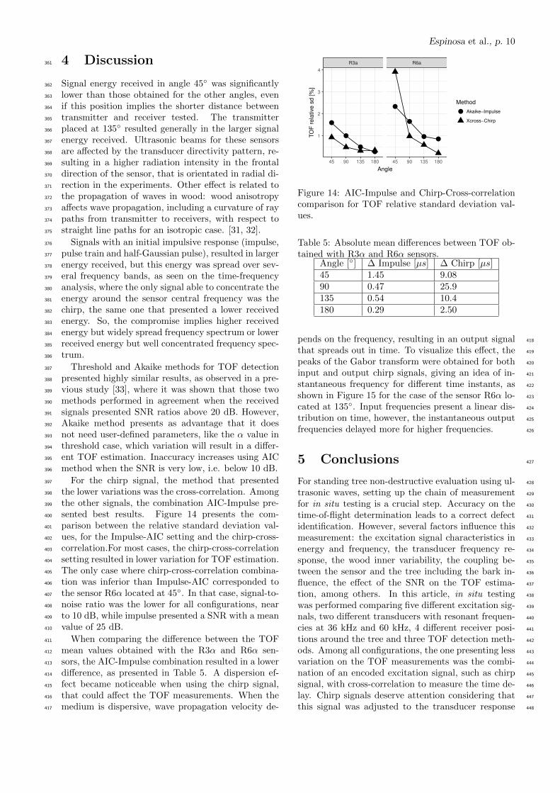
For the chirp signal, the method that presented397

the lower variations was the cross-correlation. Among398

the other signals, the combination AIC-Impulse pre-399

sented best results. Figure 14 presents the com-400

parison between the relative standard deviation val-401

ues, for the Impulse-AIC setting and the chirp-cross-402

correlation.For most cases, the chirp-cross-correlation403

setting resulted in lower variation for TOF estimation.404

The only case where chirp-cross-correlation combina-405

tion was inferior than Impulse-AIC corresponded to406

the sensor R6α located at 45◦. In that case, signal-to-407

noise ratio was the lower for all configurations, near408

to 10 dB, while impulse presented a SNR with a mean409

value of 25 dB.410

When comparing the difference between the TOF411

mean values obtained with the R3α and R6α sen-412

sors, the AIC-Impulse combination resulted in a lower413

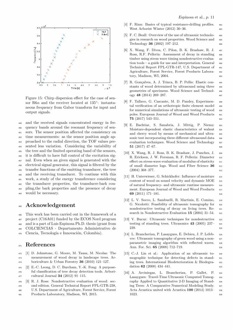
difference, as presented in Table 5. A dispersion ef-414

fect became noticeable when using the chirp signal,415

that could affect the TOF measurements. When the416

medium is dispersive, wave propagation velocity de-417

R3a R6a

45 90 135 180 45 90 135 180

1

2

3

4

Angle

TO

F r

ela

tive

sd

[%

]

Method

Akaike−Impulse

Xcross−Chirp

Figure 14: AIC-Impulse and Chirp-Cross-correlationcomparison for TOF relative standard deviation val-ues.

Table 5: Absolute mean differences between TOF ob-tained with R3α and R6α sensors.

Angle [◦] ∆ Impulse [µs] ∆ Chirp [µs]45 1.45 9.0890 0.47 25.9135 0.54 10.4180 0.29 2.50

pends on the frequency, resulting in an output signal 418

that spreads out in time. To visualize this effect, the 419

peaks of the Gabor transform were obtained for both 420

input and output chirp signals, giving an idea of in- 421

stantaneous frequency for different time instants, as 422

shown in Figure 15 for the case of the sensor R6α lo- 423

cated at 135◦. Input frequencies present a linear dis- 424

tribution on time, however, the instantaneous output 425

frequencies delayed more for higher frequencies. 426

5 Conclusions 427

For standing tree non-destructive evaluation using ul- 428

trasonic waves, setting up the chain of measurement 429

for in situ testing is a crucial step. Accuracy on the 430

time-of-flight determination leads to a correct defect 431

identification. However, several factors influence this 432

measurement: the excitation signal characteristics in 433

energy and frequency, the transducer frequency re- 434

sponse, the wood inner variability, the coupling be- 435

tween the sensor and the tree including the bark in- 436

fluence, the effect of the SNR on the TOF estima- 437

tion, among others. In this article, in situ testing 438

was performed comparing five different excitation sig- 439

nals, two different transducers with resonant frequen- 440

cies at 36 kHz and 60 kHz, 4 different receiver posi- 441

tions around the tree and three TOF detection meth- 442

ods. Among all configurations, the one presenting less 443

variation on the TOF measurements was the combi- 444

nation of an encoded excitation signal, such as chirp 445

signal, with cross-correlation to measure the time de- 446

lay. Chirp signals deserve attention considering that 447

this signal was adjusted to the transducer response 448


Figure 15: Chirp dispersion effect for the case of sen-sor R6α and the receiver located at 135◦: instanta-neous frequency from Gabor transform for input andoutput signals.

and the received signals concentrated energy in fre-449

quency bands around the resonant frequency of sen-450

sors. The sensor position affected the consistency on451

time measurements: as the sensor position angle ap-452

proached to the radial direction, the TOF values pre-453

sented less variation. Considering the variability of454

the tree and the limited operating band of the sensors,455

it is difficult to have full control of the excitation sig-456

nal. Even when an given signal is generated with the457

electrical signal generator, this signal is filtered by the458

transfer functions of the emitting transducer, the tree459

and the receiving transducer. To continue with this460

work, a study of the energy transference considering461

the transducer properties, the transducer-bark cou-462

pling,the bark properties and the presence of decay463

would be necessary.464

Acknowledgement465

This work has been carried out in the framework of a466

project (C16A01) funded by the ECOS Nord program467

and is a part of Luis Espinosa Ph.D. thesis (grant from468

COLCIENCIAS - Departamento Administrativo de469

Ciencia, Tecnologıa e Innovacion, Colombia).470

References471

[1] D. Johnstone, G. Moore, M. Tausz, M. Nicolas: The472

measurement of wood decay in landscape trees. Ar-473

boriculture & Urban Forestry 36 (2010) 121–127.474

[2] E.-C. Leong, D. C. Burcham, Y.-K. Fong: A purpose-475

ful classification of tree decay detection tools. Arbori-476

cultural Journal 34 (2012) 91–115.477

[3] R. J. Ross: Nondestructive evaluation of wood: sec-478

ond edition. General Technical Report FPL-GTR-238,479

U.S. Department of Agriculture, Forest Service, Forest480

Products Laboratory, Madison, WI, 2015.481

[4] F. Rinn: Basics of typical resistance-drilling profiles. 482

West Arborist Winter (2012) 30–36. 483

[5] F. C. Beall: Overview of the use of ultrasonic technolo- 484

gies in research on wood properties. Wood Science and 485

Technology 36 (2002) 197–212. 486

[6] X. Wang, F. Divos, C. Pilon, B. K. Brashaw, R. J. 487

Ross, R.F. Pellerin: Assessment of decay in standing 488

timber using stress wave timing nondestructive evalua- 489

tion tools – a guide for use and interpretation. General 490

Technical Report FPL-GTR-147, U.S. Department of 491

Agriculture, Forest Service, Forest Products Labora- 492

tory, Madison, WI, 2004. 493

[7] R. Goncalves, A. J. Trinca, B. P. Pellis: Elastic con- 494

stants of wood determined by ultrasound using three 495

geometries of specimens. Wood Science and Technol- 496

ogy 48 (2014) 269–287. 497

[8] F. Tallavo, G. Cascante, M. D. Pandey, Experimen- 498

tal verification of an orthotropic finite element model 499

for numerical simulations of ultrasonic testing of wood 500

poles. European Journal of Wood and Wood Products 501

75 (2017) 543–551. 502

[9] E. Bachtiar, S. Sanabria, J. Mittig, P. Niemz: 503

Moisture-dependent elastic characteristics of walnut 504

and cherry wood by means of mechanical and ultra- 505

sonic test incorporating three different ultrasound data 506

evaluation techniques. Wood Science and Technology 507

51 (2017) 47–67. 508

[10] X. Wang, R. J. Ross, B. K. Brashaw, J. Punches, J. 509

R. Erickson, J. W. Forsman, R. F. Pellerin: Diameter 510

effect on stress-wave evaluation of modulus of elasticity 511

of small diameter logs. Wood and Fiber Science 36 512

(2004) 368–377. 513

[11] H. Unterwieser, G. Schickhofer: Influence of moisture 514

content of wood on sound velocity and dynamic MOE 515

of natural frequency- and ultrasonic runtime measure- 516

ment. European Journal of Wood and Wood Products 517

69 (2011) 171–181. 518

[12] L. V. Socco, L. Sambuelli, R. Martinis, E. Comino, 519

G. Nicolotti: Feasibility of ultrasonic tomography for 520

nondestructive testing of decay on living trees. Re- 521

search in Nondestructive Evaluation 15 (2004) 31–54. 522

[13] V. Bucur: Ultrasonic techniques for nondestructive 523

testing of standing trees. Ultrasonics 43 (2005) 237– 524

239. 525

[14] L. Brancheriau, P. Lasaygues, E. Debieu, J. P. Lefeb- 526

vre: Ultrasonic tomography of green wood using a non- 527

parametric imaging algorithm with reflected waves. 528

Ann. For. Sci. 65 (2008) 712–719. 529

[15] C.-J. Lin et al.: Application of an ultrasonic to- 530

mographic technique for detecting defects in stand- 531

ing trees. International Biodeterioration & Biodegra- 532

dation 62 (2008) 434–441. 533

[16] A. Arciniegas, L. Brancheriau, P. Gallet, P. 534

Lasaygues: Travel-Time Ultrasonic Computed Tomog- 535

raphy Applied to Quantitative 2-D Imaging of Stand- 536

ing Trees: A Comparative Numerical Modeling Study. 537

Acta Acustica united with Acustica 100 (2014) 1013– 538

1023. 539


[17] A. J. Trinca, S. Palma, R. Goncalves: Monitoring540

of wood degradation caused by fungi using ultrasonic541

tomography. Proceedings of 19th international sym-542

posium on non-destructive testing of wood, Rio de543

Janeiro, Brazil, 2015, 15–21.544

[18] K. Yamashita, T. Yamada, Y. Ota, H. Yonezawa,545

I. Tokue: Detecting defects in standing trees by an546

acoustic wave tomography with pseudorandom binary547

sequence code: simulation of defects using artificial548

cavity. Proceedings of 19th international symposium549

on non-destructive testing of wood, Rio de Janeiro,550

Brazil, 2015, 542–546.551

[19] A. Arciniegas, F. Prieto, L. Brancheriau, P.552

Lasaygues: Literature review of acoustic and ultra-553

sonic tomography in standing trees. Trees 28 (2014)554

1559–1567.555

[20] V. Bucur: Acoustics of Wood. Springer-Verlag,556

Berlin/Heidelberg, Germany, 2006.557

[21] M. Loosvelt, P. Lasaygues: A Wavelet-Based Pro-558

cessing method for simultaneously determining ultra-559

sonic velocity and material thickness. Ultrasonics 51560

(2011) 325–339.561

[22] L. Brancheriau, A. Ghodrati, P. Gallet, P. Thaunay,562

P. Lasaygues: Application of ultrasonic tomography563

to characterize the mechanical state of standing trees564

(Picea abies). J. Phys.: Conf. Ser. 353 (2012).565

[23] R. Sleeman, T. van Eck: Robust automatic P-phase566

picking: an on-line implementation in the analysis567

of broadband seismogram recordings. Physics of the568

Earth and Planetary Interiors 113 (1999) 265–275.569

[24] H. Zhang: Automatic P-Wave Arrival Detection and570

Picking with Multiscale Wavelet Analysis for Single-571

Component Recordings. Bulletin of the Seismological572

Society of America 93 (2003) 1904–1912.573

[25] J. H. Kurz, C. U. Grosse, H.-W. Reinhardt: Strate-574

gies for reliable automatic onset time picking of acous-575

tic emissions and of ultrasound signals in concrete. Ul-576

trasonics 43 (2005) 538–546.577

[26] M. H. Pedersen, T. X. Misaridis, J. A. Jensen: Clini-578

cal evaluation of chirp-coded excitation in medical ul-579

trasound. Ultrasound in Medicine & Biology 29 (2003)580

895–905.581

[27] J. Rouyer, S. Mensah, C. Vasseur, P. Lasaygues: The582

benefits of compression methods in acoustic coherence583

tomography. Ultrason Imaging 37 (2015) 205–223.584

[28] P. Lasaygues, A. Arciniegas, L. Brancheriau: Use of a585

Chirp-coded Excitation Method in Order to Improve586

Geometrical and Acoustical Measurements in Wood587

Specimen. Physics Procedia 70 (2015) 348–351.588

[29] S. Qian, D. Chen: Joint time-frequency analysis.589

IEEE Signal Processing Magazine 16 (1999) 52–67.590

[30] R. Carmona, W. L. Hwang, B. TorrA c©sani: Practi-591

cal Time-Frequency Analysis. Academic Press, 1998.592

[31] S. Schubert, D. Gsell, J. Dual, M. Motavalli, P.593

Niemz: Acoustic wood tomography on trees and the594

challenge of wood heterogeneity. Holzforschung 63595

(2008) 107–112.596

[32] S. Gao, N. Wang, L. Wang, J. Han: Application of an 597

ultrasonic wave propagation field in the quantitative 598

identification of cavity defect of log disc. Computers 599

and Electronics in Agriculture 108 (2014) 123–129. 600

[33] A. Arciniegas, L. Brancheriau, P. Lasaygues: Tomog- 601

raphy in standing trees: revisiting the determination 602

of acoustic wave velocity. Annals of Forest Science 72 603

(2015) 685–691. 604

Documents

Accuracy on the Time-of-Flight Estimation for Ultrasonic