Accuracy assessment of digital elevation model using ... · Accuracy assessment of digital elevation model using stochastic simulation Annamaria Castrignanò 1 , Gabriele Buttafuoco

7th International Symposium on Spatial Accuracy Assessment in Natural Resources and Environmental Sciences. Edited by M. Caetano and M. Painho.

490

Accuracy assessment of digital elevation model using stochastic simulation

Annamaria Castrignanò1, Gabriele Buttafuoco2, Roberto Comolli3 and Cristiano Ballabio3 1 CRA - Agronomic Research Institute Via Celso Ulpiani, 5 - 70125 Bari, Italy Tel.: + 39 080 5475024; Fax: + 39 080 5475023 [email protected]

2 CNR - Institute for Agricultural and Forest Systems in the Mediterranean Via Cavour, 4-6 - 87030 Rende (CS), Italy, Tel.: + 39 0984 466036; Fax: + 39 0984 466052 [email protected]

3 Department of Environmental Sciences (DISAT), University of Milano-Bicocca Piazza della Scienza 1 - 20126 Milano, Italy Tel.: + 39 02 64482875; Fax: + 39 02 64482994 [email protected]

Abstract Various methods have been applied to generate Digital Elevation Models (DEM) but whatever method is used, DEM estimates will always be affected by errors. Comparing interpolated values with the actual elevation values, obtained with a high precision field survey, allows us to assess DEM accuracy. At every spot height location it is possible to subtract the actual values from the DEM values to obtain the error at that point. Using this error information, different types of statistics can be computed; however, Root Mean Squared Error (RMSE) is the standard measure of error used by surveyors around the world. Such a way of error reporting uses a single value for the whole DEM and makes several implicit and unacceptable assumptions about the error: it has no spatial distribution and is statistically stationary across a region. An alternative approach is proposed here to achieve an improved estimate of local error. It is based on error modelling using conditional stochastic simulations to produce alternative values of the data and so result in a probabilistic assessment of DEM accuracy. The study area is a doline of about 1.5 ha in size and is located in the Alps (North Italy) at a mean elevation of 1900 m above sea level. In this study, to test the accuracy of a previously generated DEM, elevation data were measured at 110 randomly distributed points using a laser distance system linked with an electronic theodolite. Five hundred simulations were generated using conditional and sequential Gaussian simulation algorithms. Statistical information was extracted from the set of simulated error images: 1) averaging the values for each pixel and producing the map of the ‘expected’ error in any considered location and that of standard deviation; 2) counting the number of times that each pixel exceeded the null value and converting the sum to a proportion, in order to produce the probability maps of overestimation and underestimation. Basic statistics and the histogram of errors showed them to be of approximately normal distribution with a small positive bias. The map of the expected values revealed a clear correlation of errors in the DEM to the slope of the land surface. The highest values were localised on the steepest areas in the northern half of the doline. The spatial distribution of errors was not random but showed a high probability for overestimation in the northern area, while an actual probability for underestimation was restricted to the southern area. Multiple DEM results generated by incorporating different images of the error field also allow us to derive a probable version of the products used for subsequent decision-making processes.


491

Keywords: digital elevation model, geostatistics, stochastic simulation, accuracy

1 Introduction Digital Elevation Models (DEM) have become very popular in the last two decades to describe the topographic surface and model relationships between different components of the landscape (Florinsky et al., 2002). DEMs can be produced in a number of different ways (Weibel and Heller, 1991), most of them by direct field measurements of elevations at specific locations or by photogrammetry. More specifically, in many grid-based DEMs most values are interpolated because the elevations measured in the field very seldom coincide with grid-intersections. Whatever method is used, DEM estimates will always be affected by several sources of errors (sampling, measurement, interpolation, etc.). An error can be defined as the deviation between the measurement made on the ground at the location specified and the corresponding DEM estimate. As DEM source data and production methods are not perfect a consequent mismatch will occur between observations and DEM-reported elevation values. These mismatches can be measured at control or calibration points, where elevation is determined using high accuracy measurement devices, such as GPS device or laser distance systems. Local accuracy can then be determined at any control location and generally varies as a function of coordinates within the study area. Traditionally DEM errors are reported by summary statistics, using a single value, such as the root mean square error (RMSE), which quantifies the average deviation between ground-based observation and DEM value at the set of control locations. However, such statistics are global measures of DEM accuracy and are not specific to any particular location. Therefore a user must assume that the error rates are the same everywhere, from the highest sub areas to the flattest ones. Moreover, they cannot give any indication about where the DEM errors are more likely; an additional sampling could improve the accuracy of DEM.

Moreover, in many earth and environmental science applications DEMs serve as input for detailed spatial models aimed at the determination of water consumes or the classification of terrain for suitability assessment. Given that errors occur in elevation information, there is some risk that the output of the model will be incorrect. It is thus important to test the probability of an incorrect outcome of the model to make it significant for the particular application under study. To use spatial models in a predictive way, the effect of the elevation error on the results of a spatial analysis needs to be established after which it is necessary to model the error. Such a model allows us to produce alternative versions of the input data and so derive multiple versions of the outcome; it is on this that the probability of the analysis being incorrect has to be evaluated (Hunter and Goodchild, 1997; Heuvelink, 1998). The simplest error model can be defined by drawing random values from a normal distribution which has mean and standard deviations calculated from the set of spot heights surveyed separately from the DEM information. Typically, the error is assumed to be uncorrelated to the reference elevation, which means that error magnitude and its variance are the same irrespective of whether the elevation is high or low, a property called homoscedasticity (Goovaerts, 1997). This assumption is too naïve and is not generally appropriate for modelling errors in DEMs, because higher errors are expected in areas of rugged terrain, i.e. error and terrain slope are positively correlated (Hunter and Goodchild, 1997; Veregin, 1997). A more realistic approach is directly simulating the error field (DEM-reported minus measured elevation) with spatial autocorrelation matching the experimental variogram using geostatistics. Conditional stochastic simulation is a technique in the geostatistical toolkit which


492

amounts to generating multiple realizations of spatially autocorrelated error fields with the error at locations of unchanged spot height observations. This paper is aimed at presenting an improved modelling of elevation error based on geostatistics and showing its advantages over the usual reporting of DEM errors. The method is applied to a study area in North Italy using a grid-base DEM previously created from an independent data set of direct measurements of elevations at specific locations which are then interpolated at the grid intersections.

2 Materials and Methods Case Study area

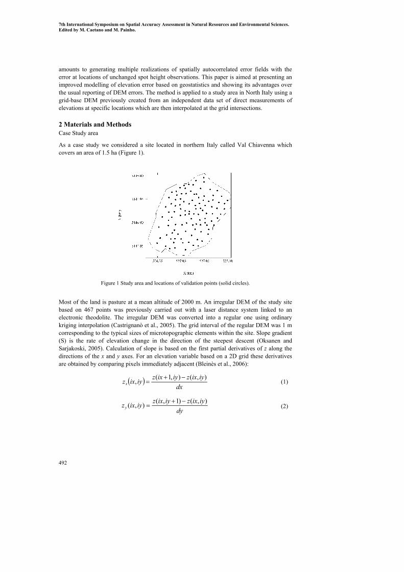
As a case study we considered a site located in northern Italy called Val Chiavenna which covers an area of 1.5 ha (Figure 1).

Figure 1 Study area and locations of validation points (solid circles).

Most of the land is pasture at a mean altitude of 2000 m. An irregular DEM of the study site based on 467 points was previously carried out with a laser distance system linked to an electronic theodolite. The irregular DEM was converted into a regular one using ordinary kriging interpolation (Castrignanò et al., 2005). The grid interval of the regular DEM was 1 m corresponding to the typical sizes of microtopographic elements within the site. Slope gradient (S) is the rate of elevation change in the direction of the steepest descent (Oksanen and Sarjakoski, 2005). Calculation of slope is based on the first partial derivatives of z along the directions of the x and y axes. For an elevation variable based on a 2D grid these derivatives are obtained by comparing pixels immediately adjacent (Bleinès et al., 2006):

( )dx

iyixziyixziyixzx),(),1(, −+

= (1)

dyiyixziyixziyixzy

),()1,(),( −+= (2)


493

where ),( iyixz is the elevation at the node ),( iyix , ),( iyixzx and ),( iyixzy are the partial

derivatives along the x axis and y axis, respectively, dx and dy are the meshes of the grid along the x axis and the y axis, respectively. According to the previous definitions, slope is calculated as:

dyiyixziyixz

dxiyixziyixziyixS ),()1,(),(),1(),( −+

+−+

= (3)

Where slope is expressed in length unit.

An independent data set of 110 spot heights (randomly surveyed with the same measurement equipment but not used in the DEM) was used to yield the error at the point by subtracting the actual value from the DEM value. Using this error information, different types of basic statistics were computed.

In addition to statistical summaries, stochastic conditional simulation was performed to generate 500 alternative equi-probable images of the unknown elevation errors using the 110 actual errors at the specific control points. Stochastic sequential simulation estimates the conditional cumulative distribution functions (CDFs) at each location using neighbouring sample data and neighbouring estimates obtained previously. The conditional CDFs can be estimated in the simplest way if a multi-Gaussian model is assumed for the multivariate distribution. Therefore, if the data of the variables are not distributed normally, a normal score transform must be performed so that transformed data have zero means and unit variances. The simulation results must then be back-transformed to the raw distribution.

Simulations were generated using a conditional sequential Gaussian simulation algorithm (Deutsch and Journal, 1998; Castrignanò and Buttafuoco, 2004), which involves defining a random path through the DEM-grid, so that each node is visited once and only once. At each unsampled location normal score transformed data values are used to estimate the probability distribution function. A random value is drawn from it as a possible simulation of a variable at that location and its value is added to the conditioning data set; the calculation proceeds for the remaining variables and then shifts to the next node along the whole random path through the grid. Several simulations can be produced, differing only in the random-number seed used for initiating simulation processes, and are virtually identical in their statistical character.

Statistical information was extracted from the set of the simulated images: 1) averaging the values for each pixel and producing the map of the “expected” error at any considered position (E-type or Expected-value estimate) (Journel, 1983) and 2) counting the number of times that each pixel exceeded or did not exceed the null value and converting the sum to a proportion in order to produce the probability maps of overestimation and underestimation, respectively.

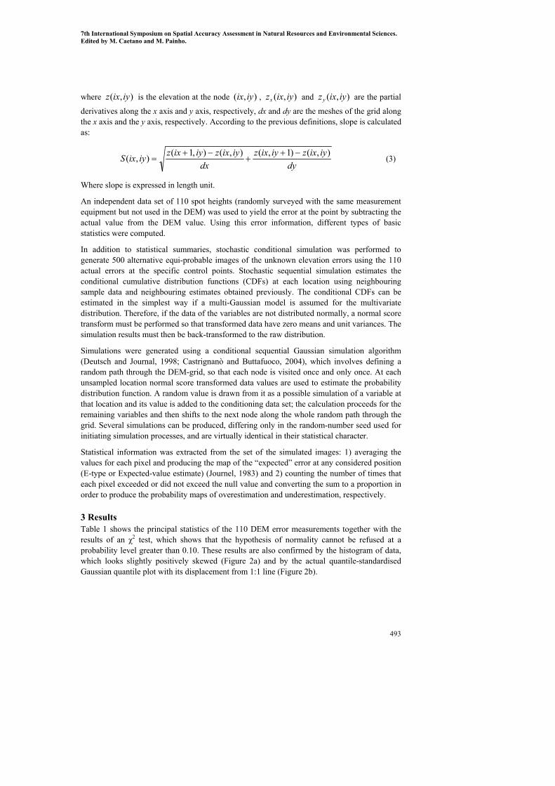
3 Results Table 1 shows the principal statistics of the 110 DEM error measurements together with the results of an χ2 test, which shows that the hypothesis of normality cannot be refused at a probability level greater than 0.10. These results are also confirmed by the histogram of data, which looks slightly positively skewed (Figure 2a) and by the actual quantile-standardised Gaussian quantile plot with its displacement from 1:1 line (Figure 2b).


494

Table 1 Basic statistics of the DEM errors. Results of the 2χ test are also reported.

Count 110

Mean (m) 0.77

Standard Deviation (m) 0.81

Variance (m2) 0.65

Maximum (m) 3.13

Median (m) 0.70

Minimum (m) -1.79

Skewness (-) 0.26

Kurtosis (-) 3.96

Experimental 2χ (-) 16.40

Theoretical 2

10.0χ (-) 21.06

Figure 2 Histogram of errors (a) and test for normality (b).

These summary statistics show that the accuracy of the DEM was quite high with a RMSE less than 1 m. However the RSME, used by most surveyors around the world as the standard measure of DEM error, is based on several unjustified assumptions, such as its value is constant or spatially stationary over the study area. These are both unrealistic assumptions and there is no possible justification for either, except simplicity. Moreover, there is no information on the actual spatial distribution and autocorrelation of error. To achieve an improved local estimate of the error the actual errors at the 110 locations were used to model spatial autocorrelation. To check the behaviour of error in terms of anisotropy a variogram map (not shown) was calculated, which did not show any significative difference as a function of direction. A bounded isotropic variogram model was then assumed, including three basic structures: a nugget effect and two spherical models, at short (18.07 m) and long (90.14 m) range. The spherical model (Webster and Oliver, 2001) is the function:


495

⎪⎩

⎪⎨

⎧

>=

≤⎥⎥⎦

⎤

⎢⎢⎣

⎡⎟⎠⎞

⎜⎝⎛−=

ahCh

ahah

ahCh

for )γ(

for 21

23)γ(

3

(5)

where C is the sill and a the range. The choice of these particular ranges was based on the complexity of the morphology of the doline and was shaped by several processes acting at multi scales.

The goodness of fitting was verified by cross validation, which reported no significant bias (mean error= -0.008), even if the variance of the standardised error was significantly different from 1 (0.85), which means that the theoretical error variance was greater than the sample one. A probable explanation may be that due to the relatively small number of control points, the sample variance of errors underestimates the population variance.

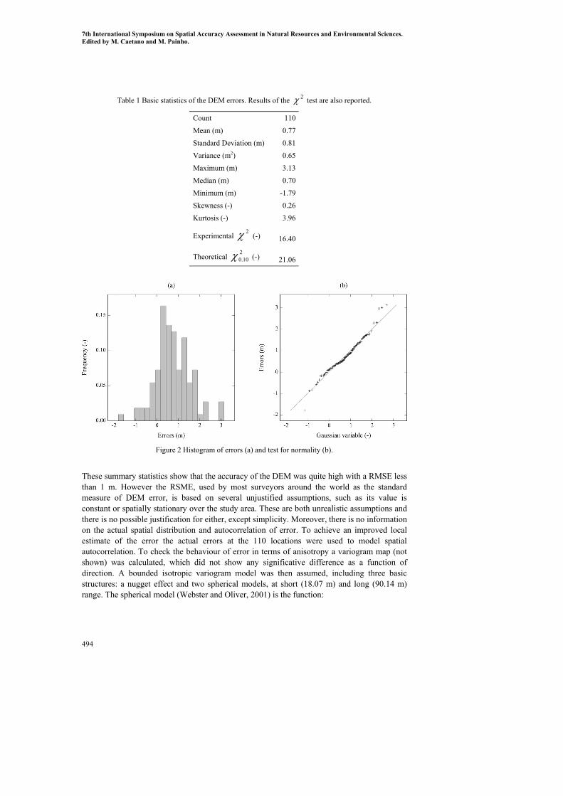
The above variogram model was used to produce the 500 simulations and the expected values of error were then mapped (Figure 3), showing the spatial distribution of errors.

Figure 3 Map of mean elevation errors.

A visual inspection of the map reveals a clear correlation of errors in the DEM with the slope of the land surface (Figure 4) reporting the highest values on the steepest areas in the northern half of the doline.


496

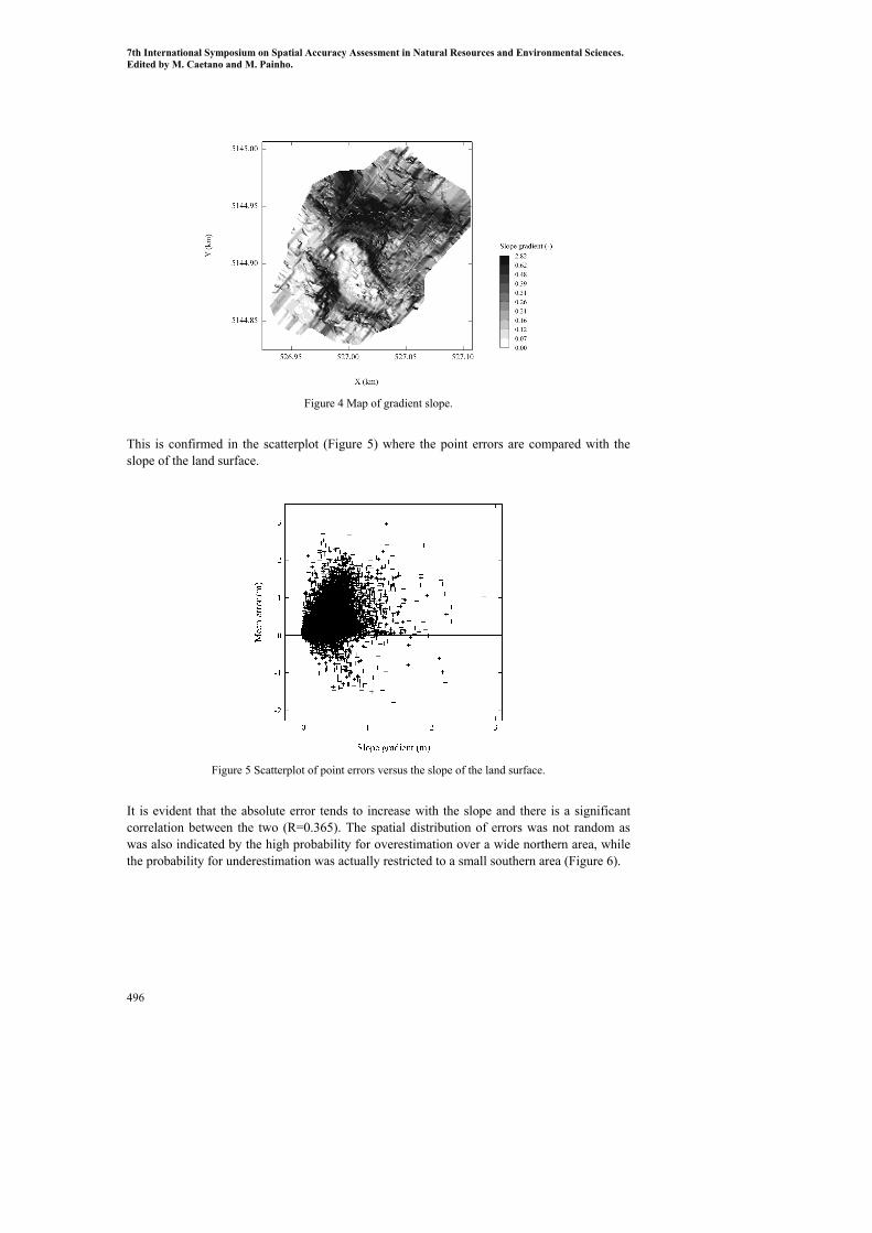
Figure 4 Map of gradient slope.

This is confirmed in the scatterplot (Figure 5) where the point errors are compared with the slope of the land surface.

Figure 5 Scatterplot of point errors versus the slope of the land surface.

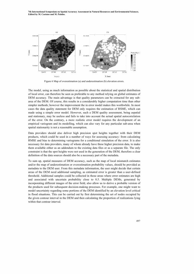
It is evident that the absolute error tends to increase with the slope and there is a significant correlation between the two (R=0.365). The spatial distribution of errors was not random as was also indicated by the high probability for overestimation over a wide northern area, while the probability for underestimation was actually restricted to a small southern area (Figure 6).


497

Figure 6 Map of overestimation (a) and underestimation (b) elevation errors.

The model, using as much information as possible about the statistical and spatial distribution of local error, can therefore be seen as preferable to any method relying on global estimates of DEM accuracy. The main advantage is that quality parameters can be extracted for any sub-area of the DEM. Of course, this results in a considerably higher computation time than other simpler methods; however the improvement the in error model makes this worthwhile. In most cases the data quality statement for DEM only requires the estimation of RSME, which can made using a simple error model. However, such a DEM quality assessment, being aspatial and stationary, may be useless and fails to take into account the actual spatial autocorrelation of the error. On the contrary, a more realistic error model requires the development of an empirical variogram and its modelling, which can also vary for any particular sub-area when spatial stationarity is not a reasonable assumption.

Data providers should also deliver high precision spot heights together with their DEM products, which could be used in a number of ways for assessing accuracy: from calculating RMSE and bias to determining variograms for a conditional simulation of the error. It is also necessary for data providers, many of whom already have these higher precision data, to make them available either as an addendum to the existing data files or as a separate file. The only constraint is that the spot heights were not used in the generation of the DEM, therefore a clear definition of the data sources should also be a necessary part of the metadata.

To sum up, spatial measures of DEM accuracy, such as the map of local mismatch estimates and/or the map of underestimation or overestimation probability values, should be provided as metadata to the DEM user. From this metadata information, the user might decide that certain areas of the DEM need additional sampling, as estimated error is greater than a user-defined threshold. Additional samples could be collected in those areas where error estimates are high and associated with uncertain probability close to 0.5. Multiple DEMs, generated by incorporating different images of the error field, also allow us to derive a probable version of the products used for subsequent decision-making processes. For example, one might want to model uncertainty regarding some portions of the DEM identified by an elevation level critical in flood situations. This can be carried out by first determining the set of nodes occupied by the given contour interval in the DEM and then calculating the proportion of realizations lying within that contour interval.


498

4 Conclusions A geostatistical approach of accuracy assessment in DEMs has been presented in this paper. Sparse reference elevation measurements were combined with DEM-estimated elevations to calculate a local mismatch. This data set of errors was then used to construct local uncertainty models for the unknown error at each DEM node. Simulated realizations of the error were generated by the Monte Carlo-type process drawing from these local uncertainty models and were used to construct spatial measures of DEM accuracy, for example probability maps of over or under-estimation. The best way to check the DEM quality is to evaluate the results in terms of probabilities, the estimation of which is based on a spatially distributed model of error using conditional stochastic simulation. The method used can be implemented in some geostatistical packages loosely coupled to GIS; in this way it could be adopted immediately to become part of the standard GIS toolkit.

References Bleinès, C., Deraisme, J., Geoffrey, F., Jeannée, N., Perseval, S., Rambert, F., Renard, D., Torres, O. and Touffait, Y., 2006, Isatis Technical References, version 6.0.0. Géovariances & École des Mines de Paris, Avon. Castrignanò, A. and Buttafuoco, G., 2004, Geostatistical Stochastic Simulation of Soil Water Content in a Forested Area of South Italy. Biosystems Engineering 87(2), pp. 257-266. Castrignanò, A., Comolli, R., Lopez, N., Buttafuoco, G. and Castrignanò, A., 2005, Using digital terrain modelling for the estimation of soil properties. Submitted to the Special Issue of Geoderma on Pedometrics 2005. Deutsch, C. V. and Journel, A. G., 1998, GSLIB: Geostatistical Software Library and User’s Guide, New York: Oxford Universi vty Press. Florinsky, I., Eilers, R., Manning, G., Fuller, L., 2002, Prediction of soil properties by digital terrain modelling. Environmental Modelling and Software 17, pp. 295-311. Goovaerts, P., 1997, Geostatistics for Natural Resources Evaluation, New York, Oxford University Press. Heuvelink, G. B. M., 1998, Error Propagation in Environmental Modelling with GIS, London, Taylor & Francis. Hunter, G. J. and Goodchild, M.F., 1997, Modelling the Uncertainty of Slope Gradient and Aspect Estimates in Spatial Databases. Geographical Analysis, 29 (1), pp. 35-49. Journel, A. G., 1983, Non-parametric estimation of spatial distributions. Mathematical Geology, 15, pp. 445-468. Oksanen, J. and T. Sarjakoski, 2005, Error propagation of DEM-based surface derivatives, Computers & Geosciences 31, pp. 1015-1027. Veregin, H., 1997, The Effects of Vertical Error in Digital Elevation Models on the Determination of Flow-path Direction. Cartography and Geographic Information Systems, 24 (2), pp. 67-79. Webster, R. and Oliver, M. A., 2001, Geostatistics for Environmental Scientists, Chichester, Wiley. Weibel, R. and Heller, M., 1991, Digital Terrain Modeling. In Geographical Information Systems: Principles and Applications, D. J. Maguire, M. F. Goodchild and D. W. Rhind (eds.), pp. 269-297, London: Longman.

Documents

Accuracy assessment of digital elevation model using ... · Accuracy assessment of digital elevation model using stochastic simulation Annamaria Castrignanò 1 , Gabriele Buttafuoco